FBA.tex

FOUNDATION BLOCK(A) INTRODUCTION TO PROBABILITY

AND STATISTICS

1 PROBABILITY

1.1 Multiple approaches

The concept of probability may be defined and interpreted in several different ways, the chief ones arisingfrom the following four approaches.

1.1.1 The classical approach

A game of chance has a finite number of different possible outcomes, which by symmetry are assumed‘equally likely’. The probability of any event (i.e. particular outcome of interest) is then defined as theproportion of the total number of possible outcomes for which that event does occur.Evaluating probabilities in this framework involves counting methods (e.g. permutations and combina-tions).

1.1.2 The frequency approach

An experiment can be repeated indefinitely under essentially identical conditions, but the observedoutcome is random (not the same every time). Empirical evidence suggests that the proportion of timesany particular event has occurred, i.e. its relative frequency, converges to a limit as the number ofrepetitions increases. This limit is called the probability of the event.

1.1.3 The subjective approach

In this approach, an event is a statement which may or may not be true, and the (subjective) probabilityof the event is a measure of the degree of belief which the subject has in the truth of the statement. Ifwe imagine that a ‘prize’ is available if and only if the statement does turn out to be true, the subjectiveprobability can be thought of as the proportion of the prize money which the subject is prepared togamble in the hope of winning the prize.

1.1.4 The logical approach

Formal logic depends on relationships of the kind A −→ B (‘A implies B’) between propositions. The log-ical approach to probability generalizes the concept of implication to partial implication; the conditionalprobability of B given A measures the extent to which A implies B. In this approach, all probabilitiesare ‘conditional’; there are no ‘absolute’ probabilities.

Some pro’s and con’s of four approaches:

Classical Frequency Subjective LogicalCalculation Objective and Applicable to Extends formal

PRO straight-forward empirical wide range logic inof ‘events’ consistent way

Limited Depends on Depends on Yields no wayCON in scope infinite individual of assigning

repeatability probabilities

1.2 Axiomatic probability theory

Because there is not a uniquely best way of defining probabilities, it is customary to lay down a setof rules (axioms) which we expect probabilities to obey (whichever interpretation is put on them). A

1

mathematical theory can then be developed from these rules. The framework is as follows. For anyprobability model we require a probability space (Ω, F, P) with

• the set Ω of all possible outcomes, known as the sample space (for the game, experiment, etc.)

• a collection F of subsets of Ω, each subset being called an event (i.e. the event that the observedoutcome lies in that subset).

• a probability measure defined as a real valued function P of the elements of F (the events) satisfyingthe following axioms of probability:

A1. P(A)≥ 0 for all A∈ FA2. P(Ω ) = 1A3. If A1, A2,... are mutually exclusive events (i.e. have no elements in common), then P (A1 ∪A2 ∪ ...) = P (A1) + P (A2) + ... [The sum may be finite or infinite].

Example

In a ‘classical’ probability model, Ω consists of the n equally likely outcomes a1, a2, ..., an say, F consistsof all subsets of Ω, and P is defined by

P (A) =no. of elements in A

nfor A ∈ F.

It is easy to show that the P satisfies the axioms of probability.

Theorems about probabilities may be proved using the axioms. The following is a simple example.

Theorem

If Ac = Ω\A, (the ‘complement’ or ‘negation’ of A), then P (Ac) = 1 − P (A).

Proof

A and Ac are mutually exclusive with union Ω. Therefore

P (A) + P (Ac) = P (Ω) (by axiom A3)= 1 (by axiom A2).

1.3 Conditional probability and independence

For any event A with P (A) > 0, we can ‘condition’ on the occurrence of A by defining a new probabilitymeasure, PA say, which is obtained from P by reducing all probability outside A to zero and rescalingthe rest so that the axioms are still satisfied. Thus for any event B in the original sample space Ω, wedefine

PA(B) =P (A ∩ B)

P (A)= probability of B conditional on A or given A

PA(B) is normally written P (B | A).Conditional probabilities are often easier to specify than unconditional ones, and the above definitionmay be rearranged to give

P (A ∩ B) = P (A)P (B | A)

which is sometimes known as the multiplication rule. This may be extended (by an easy inductionargument) to a sequence A1, A2, ..., An of events

P (A1 ∩ A2 ∩ . . . ∩ An) = P (A1)P (A2 | A1)P (A3 | A1 ∩ A2) . . . P (An | A1 ∩ . . . ∩ An−1)

which is useful when it is easy to write down the probability of each event in the sequence conditionalon all the previous ones having occurred.

2

Another important relationship involving conditional probabilities is the law of total probability (some-times known as the elimination rule). This involves the notion of a partition of the sample space, whichis a sequence A1, A2, . . . (finite or infinite) such that

A1 ∪ A2 ∪ . . . = Ω

and Ai ∩ Aj = φ whenever i 6= j. In other words, ‘A1, A2, . . . are mutually exclusive and exhaustive’or alternatively ‘one and only one of A1, A2, . . . must occur’. If A1, A2, . . . is a partition and B is anarbitrary event, then the law of total probability states that

P (B) =∑

i

P (Ai)P (B | Ai)

This follows from the axioms and the definition of conditional probability, since A1 ∩ B,A2 ∩ B, . . . aremutually exclusive with union B, and P (Ai ∩ B) = P (Ai)P (B | Ai) for each i.

Example

In a multiple choice test, each question has m possible answers. If a candidate knows the right an-swer (which happens with probability p) he gives it; if he thinks he knows it but is mistaken (whichhas probability q) he gives the answer he thinks is correct; and if he does not think he knows it (withprobability r = 1-p-q) then he chooses an answer at random. What is the probability that he answerscorrectly?A1 = knows right answerB = answers correctlyA2 = thinks he knows itA3 = does not think he knows it

P (A1) = p P (B | A1) = 1 P (A2) = q P (B | A2) = 0 P (A3) = r P (B | A3) =1

m

therefore P (B) = p.1 + q.0 + r. 1m = p + r

m .

Sometimes we wish to relate two conditional probabilities. This is easily achieved

P (A | B) =P (B ∩ A)

P (B)=

P (A ∩ B)

P (B)=

P (B | A)P (A)

P (B)

This result is known as Bayes’ Theorem (or Bayes’ rule). It is often used in conjunction with a partitionwhere we wish to know the probability of one (or more) of the events of the partition having occurredconditional on the ‘secondary event’ B having been observed to occur

P (Aj | B) =P (Aj)P (B | Aj)

P (B)=

P (Aj)P (B | Aj)

ΣP (Ai)P (B | Ai)

Example (Model as above).

What is the probability that the candidate knew the right answer given that he answered correctly?

P (A1 | B) =p.1

p.1 + q.0 + r. 1m

=p

p + rm

Bayes’ Theorem lies at the foundation of a whole branch of statistics – Bayesian statistics. See Chapter 8.

Independence

Event B is said to be independent of event A if

P (B | A) = P (B)

i.e. conditioning on A does not affect the probability of B. The relationship is more usually writtenequivalently as

P (A ∩ B) = P (A)P (B)

3

which indicates that the relationship is symmetrical: A and B are mutually independent. This form mybe generalized to longer sequences: events A1, A2, . . . are said to be (mutually) independent if

P (Ai1 ∩ Ai2 ∩ . . . ∩ Aik) = P (Ai1)P (Ai2) . . . P (Aik

)

for any finite collection of distinct subscripts i1, i2, . . . ik.

Example

For three events A, B, C to be mutually independent, all the following relationships must hold.

P (A ∩ B) = P (A)P (B)P (A ∩ C) = P (A)P (C) P (A ∩ B ∩ C) = P (A)P (B)P (C)P (B ∩ C) = P (B)P (C)

Fortunately, independence is usually used as an assumption in constructing probability models, andso we do not need to check a whole collection of relationships such as the above.

2 RANDOM VARIABLES

2.1 Definition

Often the outcome of an experiment will have numerical values, e.g. throwing a die we can take thesample space as Ω = 1, 2, 3, 4, 5, 6. In other more complicated experiments even though the outcomesmay not be numerical we may be interested in a numerical value which is a function of the observedoutcome, e.g. throwing three dice we may be interested in ‘the total score obtained’. In this latterexample, the sample space may be described as

Ω = (1, 1, 1), (1, 1, 2), (1, 1, 3), . . . . . . (6, 6, 6)

but the possible values which ‘the total score obtained’ can take are given by

ΩX = 3, 4, 5, . . . 18

which is called the induced sample space. The function which takes Ω into ΩX according to the ruledescribed is called a random variable, e.g. ‘the total score obtained’ is a random variable which we maycall X say. Associated with the sample space induced by X are:

(i) FX = events ‘generated’ by X (e.g. ‘X=4’ and ‘X is an even number’ are events);

(ii) PX = induced probability measure, known as the distribution of X, e.g. PX(3, 4) = P (X = 3 or 4) =P(1, 1, 1), (1, 1, 2), (1, 2, 1)(2, 1, 1) = 4

216 assuming dice are fair.

It is often convenient to work with (ΩX , FX , PX), rather than with (Ω, F, P ), but we have to be carefulif considering more than one random variable defined on the same underlying sample space.

2.2 Types of distribution

A random variable X, or its distribution, is called discrete if it only takes values in the integers or(possibly) some other countable set of real numbers. (This will automatically be true if the underlyingsample space is countable.) In this case the distribution is entirely specified by giving its value on everysingleton in the induced sample space:

PX(i) = pX(i) say for iǫΩX .

pX(i) is called the probability function of X (or of its distribution). The probability of any event AX in FX

is then found by summing the values of pX over the singletons contained inAX :

P (AX) =∑

iǫAX

pX(i) (∗)

4

In order to satisfy the axioms of probability, it is sufficient that the function pX satisfies

(i) pX(i) > 0 for all iǫΩX (to satisfy A1)

(ii)∑

iǫΩXpX(i) = 1 (to satisfy A2)

A3 is then automatically satisfied because of (∗).

Example

pX(i) = 1i(i+1) with ΩX = 1, 2, 3, . . . is a probability function since pX(i) > 0 obviously and also

∑∞i=1 pX(i) =

∑∞i=1(

1i − 1

i+1 ) = 1.

A random variable X, or its distribution, is called (absolutely) continuous if it takes values on thewhole real line or some sub-intervals and the probability that it lies in any interval [a,b] say is given bythe integral over the interval of a function, known as the probability density function (p.d.f.)fX :

P (a < X ≤ b) =

∫ b

a

fX(x) dx = PX((a, b]).

Note that it does not matter whether we include the endpoints of the interval or not; the probability ofany singleton is zero.In order to satisfy the axioms of probability it is sufficient that the function fX satisfies

1. fX(x) > 0 for all x;

2.∫

ΩX

fX(x)dx = 1.

Example

For what value of c is the functionfX(x) =

c

1 + x2

a p.d.f.?Obviously (i) is satisfied provided c ≥ 0; to satisfy (ii) we must have

1 =

∫ ∞

−∞

c

1 + x2dx = c[tan−1x]∞−∞ = c[

π

2− (

−π

2)] = cπ, therefore c =

1

π.

Note. Not all distributions are either discrete or absolutely continuous; for example, a distribution maybe partly discrete and partly absolutely continuous.

The distribution function FX of any distribution is defined as

FX(x) = P (X ≤ x) = PX((−∞, x]) for all real x.

If the distribution is discrete, it will be a step function:

FX(x) =∑

i≤x

pX(i) iǫΩX

whereas if the distribution is absolutely continuous, it will be a smooth function with derivative thep.d.f.:

FX(x) =

∫ x

−∞fX(u) du

therefore F ′X(x) = fX(x). Because of the axioms of probability, a distribution function is always non-

decreasing, continuous from the right, and satisfies

FX(x) ↓ 0 as x → −∞FX(x) ↑ 1 as x → +∞

5

Example

For the previous two examples, respectively,

FX(x) =

∑[x]i=1(

1i − 1

i+1 ) = 1 − 1[x]+1 for x ≥ 0 ([ ]denote ‘whole no. part of’)

0 for x < 0

and

FX(x) =∫ x

−∞1

π(1+u2)du = 12 + 1

π tan−1x (−∞ < x < ∞).

Note. In the discrete case where ΩX = 0, 1, 2, . . . say, we can ‘recover’ PX from FX using thefact that pX(i) = FX(i) − FX(i − 1) (difference of successive values).

Note. We usually drop subscripts on p, f and F if it is clear to which variable they refer.

2.3 Expectation and more general moments

If X is a random variable, then its expectation, expected value or mean EX or E(X) is the numberdefined by

EX =∑

i∈ΩXipX(i) (discrete case)

EX =∫

ΩX

xfX(x)dx (abs. cont. case)

provided that the sum or integral converges (otherwise the expectation does not exist). It is a weightedaverage of the possible values which X can take, the weights being determined by the distribution. Itmeasures where the centre of the distribution lies.

Properties

• If X > 0 always, then EX > 0.

• If X ≡ c (constant) then EX = c.

• If a and b are constants then E(a + bX) = a + bEX (linearity).

If g(X) is a function of a random variable, then, to evaluate Eg(X), it is unnecessary to know thedistribution of g(X) because it may be shown that

Eg(X) =

∑

i∈ΩXg(i)pX(i) (discrete case)

∫

ΩX

g(x)fX(x)dx (abs. cont. case)

Of particular importance are moments of a random variable, such as the following:

EXr = rth moment of X

E(X − µX)r = rth moment of X about its mean (where µX = EX)

EX(X − 1) . . . (X − r + 1) = rth factorial moment

The second moment of X about its mean is called the variance of X

var(X) = E(X − µX)2 = σ2X

and measures the extent to which the distribution is dispersed about µX . Its positive square root σX iscalled the standard deviation (s.d.).

Properties of variance

• var (X) ≥ 0, with equality iff X is a constant random variable

6

• var (a + bX) = b2 var X.

The mean and variance of a distribution are commonly used measures of ‘location’ and ‘dispersion’ butthere are other possibilities, e.g. the median is defined as any value η such that

FX(η) > 12

and FX(η−) ≤ 12 (η may not be unique)

and is a measure of location (the half-way point of the distribution); and the interquartile range is definedas η 3

4

−η 1

4

where the upper and lower quartiles η 3

4

and η 1

4

are defined as the median but with 12 replaced

by 34 and 1

4 respectively; the interquartile range is a measure of dispersion.

Examples of moments will follow in the next section.

2.4 Some standard distributions

2.4.1 The binomial distribution B(n, θ)

This is the discrete distribution with probability function given by

p(i) =

(

ni

)

θi(1 − θ)n−i for 0 ≤ i ≤ n

0 otherwise

n and θ are the parameters of the distribution. n is a positive interger and θ a real number between0 and 1. It arises as the distribution of the number of ‘successes’ in n independent ‘Bernoulli trials’ ateach of which there is probability of ‘success’ θ. A combinatorial argument leads to the above formula.If X has B(n, θ) distribution then we write X ∼ B(n, θ) and find

EX = nθ and varX = nθ(1 − θ).

2.4.2 The Poisson distribution Po(µ).

This is the discrete distribution with probability function given by

p(i) = e−µ µi

i! for i = 0, 1, 2, . . .

0 otherwise.

µ is the parameter of the distribution, and is a positive real number. It arises as the distribution ofthe number of ‘occurrences’ in a time period during which in a certain sense these ‘occurrences’ arecompletely random.

The Poisson distribution with parameter µ has mean µ and variance µ.

One way of deriving the Poisson probability function is to take the limit of B(n, θ) as n → ∞ andθ → 0 but nθ remains fixed at µ. If we substitute θ = µ

n then the binomial probability function is

n!i!(n−i)!

(

µn

)i (1 − µ

n

)n−i= n.(n−1)...(n−i+1)

n.n...nµi

i! (1 − µn )−i

(

1 − µn

)n

→ 1.µi

i! 1.e−µ as n → ∞.

For this reason, the binomial distribution B(n, θ) is well approximated by Po(nθ) when n is large and θis small.

The distribution functions of the binomial and Poisson distribution are tabulated for various valuesof the parameters (Neave tables 1.1 and 1.3(a) respectively).

7

2.4.3 The normal distribution N(µ, σ2)

The normal distribution with parameters µ and σ2 is the continuous distribution with p.d.f. given by

f(x) =1√2πσ

exp

(

− (x − µ)2

2σ2

)

for −∞ < x < ∞

It is a symmetrical bell-shaped distribution of great importance. It has mean µ and variance σ2.If X has N(µ, σ2) distribution then X−µ

σ has standard normal distribution N(0,1), whose density isgiven the special symbol φ and likewise its distribution function Φ. Both Φ and its inverse are tabulated(Neave tables 2.1, 2.3). Any probability involving a N(µ, σ2) random variable may be obtained fromthese tables, e.g.

P (a < X ≤ b) = P

(

a − µ

σ≤ X − µ

σ≤ b − µ

σ

)

= Φ

(

b − µ

σ

)

− Φ

(

a − µ

σ

)

2.4.4 The (negative) exponential distribution Ex(λ)

This is the continuous distribution with p.d.f. given by

f(x) =

λe−λx for x ≥ 0 (λ > 0)0 for x < 0

It occurs commonly as the distribution of a “waiting time” in various processes. It has mean 1λ and

variance 1λ2 . Its distribution function is given by

F (x) =∫ x

0λe−λudu = 1 − e−λx for x ≥ 0

= 0 for x < 0

2.4.5 The gamma distribution Ga(α, λ)

This is a generalization of the negative exponential distribution with p.d.f. given by

f(x) =

λα

Γ(α)xα−1e−λx for x > 0 (λ, α > 0).

0 x < 0

Here Γ(α) is the gamma function which ensures that the p.d.f. integrates to 1:

Γ(α) =∫∞0

uα−1e−udu (definition).

(NB Γ(

12

)

=√

π).) It has mean α/λ and variance α/λ2. The negative exponential is the special caseα = 1; another special case of interest in statistics is the case α = ν/2, λ = 1/2, where ν is a positiveinteger, which is known as the χ2 distribution with ν degrees of freedom, χ2

ν .

2.5 Transformations of random variables

If X is a random variable then so is Y = g(X) for any function g, and its distribution is related to thatof X by

PY (B) = P (g(X) ∈ B) = PX(g−1(B))

for BǫΩY , where g−1(B) denotes the inverse image of B under g. In many cases such inverse imagesare easy to identify, e.g. if g is a continuous increasing function and B = (−∞, y] say, then here thedistribution function of Y is given by

FY (y) = PY ((−∞, y]) = P (g(X) ≤ y) = P (X ≤ g−1(y)) = FX(g−1(y))

and if X has p.d.f. fX and g is also differentiable, then Y is also absolutely continuous with p.d.f.

f(y) = F ′Y (y) =

d

dyFX(g−1(y)) = fX(g−1(y))

d

dy[g−1(y)]

8

Example

If X has Ex(λ) distribution and Y =√

X then the above conditions are satisfied (since X ≥ 0 al-ways) and g(x) =

√x, g−1(y) = y2 for y ≥ 0.

therefore fY (y) = λe−λy2

2y

= 2λye−λy2

for y ≥ 0.

It is sometimes useful to approximate moments of functions of random variables in terms of moments ofthe original random variables as follows: suppose the distribution of X is such that the first term Taylorexpansion

g(X) = g(µ) + g′(µ)(X − µ) where µ = EX

is a good approximation over the bulk of the range of X. It then should follow that

Eg(X) = g(µ) since E(X − µ) = 0and Var g(X) = [g′(µ)]2 VarX.

This approximation will be useful if g is smooth at µ.

Example

If X has Ga(α, λ) distribution, then E(logX) ≃ log α/λ and Var(log X) ≃ ( λα )2 α

λ2 = 1α .

2.6 Independent random variables

Two random variables X and Y are said to be independent of each other if

P (XǫA, Y ǫB) = P (XǫA)P (Y ǫB)

for any choice of events A and B. This clearly extends the notion of independence of events. The gener-alization to more than two random variables follows: X1,X2, . . . (a finite or infinite sequence) are inde-pendent. If the events X1ǫA1,X2ǫA2 . . . XnǫAn are independent for all n and for all A1ǫFX1

, . . . AnǫFXn.

Often we use a sequence of independent random variables as the starting point in constructing a model.It may be shown that it is always possible to construct a probability space which can carry a sequenceof independent random variables with given distributions.

ExampleIn a sequence of n Bernoulli trials with probability of success θ , let

Uk =

1 if success occurs on kth trials (1 < k < n)0 otherwise.

Then U1, U2, . . . Un are independent (because the trials are independent) and each has the same distri-butions given by the probability function

PU (0) = 1 − θPU (1) = θPU (i) = 0 for other i.

Note also that EUk = θ and var Uk = θ(1 − θ) for each k.If we have several random variables defined on the same probability space, then we can form functionsof them and create new random variables, e.g. we can talk about the sum of them. The following resultsare important.

Properties

(i) E(X1 + X2 + . . . + Xn) = EX1 + EX2 + . . . + EXn.

If X1,X2, . . . ,Xn are independent then in addition

9

(ii) E(X1X2 . . . Xn) = (EX1)(EX2) . . . (EXn)

and

(iii) var (X1 + X2 + . . . + Xn) = var X1 + var X2 + . . . +var Xn.

Example (as above)

U1 + U2 + . . . + Un = total no. of successes which has B(n, θ) distribution.therefore

E(U1 + U2 + . . . + Un) = nθ

var(U1 + U2 + . . . + Un) = nθ(1 − θ)

confirming our earlier result for B(n, θ).

Often if each of a sequence of independent random variables has a standard form, then their sum hasa related standard form. The following summary gives examples, it being understood in each case thatthe two random variables on the left are independent, and the notation being self-explanatory.

(i) B1(n1, θ) + B2(n2, θ) = B3(n1 + n2, θ)(ii) Po1(µ1) + Po2(µ2) = Po3(µ1 + µ2)(iii) N1(µ1, σ

21) + N2(µ2, σ

22) = N3(µ1 + µ2, σ

21 + σ2

2)(iv) Ga1(α1, λ) + Ga2(α2, λ) = Ga3(α1 + α2, λ)

3 MULTIVARIATE RANDOM VARIABLES AND DISTRI-BUTIONS

3.1 General Concepts

If X1,X2, . . . ,Xk are random variables, not necessarily independent, defined on the same sample space,then the induced sample space is (a subset of) k-dimensional space, ℜk, and the induced probabil-ity measure is called the joint distribution of X1,X2, . . . ,Xk. Alternatively we can think of X =(X1,X2, . . . ,Xk)′ as a random vector.The joint distribution may be discrete, i.e. given by

P(X1,X2, . . . ,Xk)ǫB =∑

(i1,

∑

i2,...,

∑

ik)ǫB

pX1,X2,...,Xk(i1, i2, . . . , ik) (B ⊆ ℜk)

where pX1,X2,...,Xkis called the joint probability function of X1,X2, . . . ,Xk.

It may also be absolutely continuous, i.e. given by

P(X1,X2, . . . ,Xk)ǫB =

∫ ∫

B

. . .

∫

fX1,X2,...,Xk(x1, x2, . . . , xk)dx1dx2 . . . dxk

where fX1,X2,...,Xkis called the joint probability density function of X1,X2, . . . ,Xk.

There are many other possibilities, e.g. it might be discrete in the first variable and absolutely continu-ous in the second variable. For simplicity of notation we shall talk mainly about two random variables(X,Y ) say. Most of the concepts generalize naturally.

Discrete case

The joint probability function

pX,Y (i, j) = P (X = i,X = j)

must satisfy pXY (i, j) ≥ 0 and∑

i

∑

j pXY (i, j) = 1. The marginal probability function of X (i.e. itsprobability function in the usual sense) is found by summing over j while keeping i fixed:

pX(i) = ΣjpX,Y (i, j).

10

Similarly pY (j) = ΣipX,Y (i, j).

If (and only if) X and Y are independent then pX,Y factorizes into the marginals:

pX,Y (i, j) = pX(i)pY (j)

More generally we can define the conditional probability functions

pX|Y (i | j) = P (X = i | Y = j) =pX,Y (i, j)

pY (j)

and similarly the other way round. We then have, e.g.

pY (j) = ΣipX(i)pY |X(j | i)

by the law of total probability.

Absolutely continuous case

All the analagous results go through, where probability functions are replaced by p.d.f’s and sumsby integrals. The definition of conditional p.d.f. as

fX|Y (x | y) =fX,Y (x, y)

fY (y)

is less obvious but nevertheless works.

3.2 Covariance and Correlation

The covariance of two random variables X and Y is defined as

cov(X,Y ) = E(X − EX)(Y − EY ) = EXY − (EX)(EY ).

If X and Y are independent then cov(X,Y) = 0, but the converse is not true. The covariance measureshow strongly X and Y are (linearly) related to each other, but if we require a dimensionless quantity todo this we use the correlation coefficent.

ρ(X,Y ) =cov(X,Y )√

[(varX)(varY )].

It may be shown that | ρ(X,Y ) |≤ 1, with equality iff there is an exact linear relationship between Xand Y (Y ≡ a + bX say).To evaluate the covariance we use

E(XY ) = ΣjΣjijpX,Y (i, j) in the discrete case etc.

Covariance is a symmetrical function (cov(X,Y) = cov(Y,X)) and is linear in each of its arguments, e.g.

cov(X, aY + bZ) = acov(X,Y ) + bcov(X,Z).

It is needed when we wish to evaluate the variance of the sum of two (or more) not necessarily independentrandom variables:

var(X + Y ) = varX + varY + 2cov(X,Y ).

This is most easily seen by writing var(X + Y ) = cov(X + Y,X + Y ) and using the linearity in botharguments.

3.3 Conditional expectation

If X and Y are two random variables, the expected value of Y given X = x is simply the mean of theconditional distribution. It is denoted by E(Y | X = x).Since this depends upon x, we can write it as

g(x) = E(Y | X = x) say.

11

The corresponding function of the random variable X, g(X), is known as the conditional expectation ofY given X, denoted by E(Y | X). Note that it is a random variable which is a function of X but not ofY (Y has been ‘eliminated’ by summation or integration).We can similarly talk about var(Y | X). The following properties of conditional expectation are useful:

• E(E(Y | X)) = EY

• E(h(X)Y | X) = h(X)E(Y | X) (Any function of X may be ‘factorized out’.)

• var Y = var E(Y | X) + E var(Y | X).

3.4 Transformations of multivariate variables

The ideas of Section 2.5 generalize naturally. For the invertible transformation

Y1 = g1(X)...

...Yn = gn(X)

with inverseX1 = G1(Y)...

...Xn = Gn(Y)

and Jacobian (generalization of derivative)

J(y) = det

∂x1

∂y1

. . . ∂x1

∂yn

......

∂xn

∂y1

. . . ∂xn

∂yn

where J(y) 6= 0 for invertibility. It can be shown that

fY(y) = fX(G1(y), . . . , Gn(y)) | J(y) | .

Frequently, unwanted y’s must then be integrated out to obtain the marginal distribution of the Y ’s ofinterest (again, take care over the ranges of integration).A particular case in common use is the convolution integral for obtaining the distribution of the sum oftwo variables. Using the transformation U = X + Y, V = X,

fU (u) =

∫

RV |u

fX,Y (v, u − v)dv.

3.5 Standard multivariate distributions

3.5.1 The multinomial

If in each of a sequence of n independent trials, one of k different outcomes A1, A2, . . . , Ak may occur,with probabilities θ1, θ2, . . . , θk respectively (θ1 + θ2 + . . . + θk = 1) and we define

X1 = no. of times A1 occursX2 = no. of times A2 occurs

etc.

then the joint distribution of X1,X2, . . . ,Xk is called the multinomial with parameters (n; θ1, θ2, . . . , θk).A combinatorial argument gives its joint probability function as

p(i1, i2, . . . , ik) =

n!i1!i2!...ik!θ

i11 θi2

2 . . . θik

k if i1, i2, . . . , ik ≥ 0

i1 + i2 + . . . + ik = n

0 otherwise

12

The marginal distribution of Xr is B(n, θr) and the distribution of Xr +Xs is B(n, θr + θs), which leadsto the following results:

EXr = nθr

var(Xr) = nθr(1 − θr)cov(Xr,Xs) = −nθrθs if r ≥ s.

The likelihood function is given by

L(X;θ) =n!

X1!X2! . . . Xk!θX1

1 θX2

2 . . . θXk

k

(assuming X1+X2+. . .+Xk = n) and the maximum likelihood estimators are θr = Xr

n for r = 1, 2, . . . , kwhich are unbiased.

3.5.2 The multivariate normal distribution

If µ is a k-vector and Σ is a symmetric positive-definite kxk matrix, then random vector X hasmultivariate normal distribution with mean µ and covariance matrix Σ, denoted by N(µ,Σ), if the jointp.d.f. is given by

f(x) =1

(2π)n/2 | Σ |1/2exp −1

2(x − µ)′Σ−1(x − µ).

As the terminology suggests, EXr = µr for each r and cov(Xr,Xs) = σrs = (r, s) element of Σ.Despite the forbidding form of the joint p.d.f., the multivariate normal distribution has many nice prop-erties and is the natural analogue of the normal.

Properties

(i) If a is a q-vector (q ≤ k) and B is a qxk matrix of rank q then

Y = a + BX ∼ N(a + Bµ,BΣB′)

(ii) If X(1),X(2), . . . , X(n) are i.i.d. N(µ,Σ), then

X =1

n

n∑

i=1

X(i) ∼ N(µ,1

nΣ).

4 INFERENCE

4.1 Introduction

In probability theory we use the axioms of probability and their consequences as ‘rules of the game’ fordeducing what is likely to happen when an ‘experiment’ is performed. In statistics we observe the out-come of an ‘experiment’ - which we call the data - and use this as evidence to infer by what mechanismthe observation has been generated. Because of the apparent random variation in the data we assumethat this mechanism is a probability model; the data help us to reach some decision about the nature ofthis model. Often in order to make the problem of inference tractable, we make some broad assumptionsabout the form of the underlying probability model; the data then help to narrow our choices withinthese assumptions.

As a common example, a collection of data of the same type, x1, x2, ..., xn say, may be regarded as anobservation on a sequence of independent identically distributed (i.i.d.) random variables, X1,X2, ...,Xn

say, whose common distribution is of some standard form, e.g. normal or Poisson, but whose parametersare unknown. Such data constitute a random sample. The data then give us information about the likelyvalues of the parameters.

In classical inference we assume that the values of our underlying parameters are unknown, but fixed.In Chapter 5 we look at problems of this type.

In Bayesian inference we express our initial uncertainty about the true values of parameters by as-signing them probability distributions. The data then combine with these prior ideas to offer an updateddistributional assessment of the parameter values (see Chapter 8).

13

4.2 Types of (classical) inference

Three common types of inference are as follows

4.2.1 Point estimation

A single number (which is a function of the observed data) is given as an estimate of some parameter.The formula specifying the function is called an estimator.

4.2.2 Testing hypotheses

A hypothesis about a parameter value, or more generally about the underlying probability model, is tobe accepted or rejected on the basis of the observed data.

4.2.3 Interval estimation

Instead of a single number as in 4.2.1, we specify a range (usually an interval) of values in which theparameter is thought to lie on the basis of the observed data.

Many other types of action are possible, e.g. ‘collect more data’.

4.3 Sampling distributions

Inference about a population is usually conducted in terms of a statistic t = T (x1, x2, ..., xn) whichis a function of the observed data. Regarded as a function of the corresponding random variables,T = T (X1,X2, ...,Xn), this statistic is itself a random variable. Its distribution is known as the samplingdistribution of the statistic. In principle this distribution can be derived from the distribution of thedata; in practice this may or may not be possible. The sampling distribution is important because itenables us to construct good inferential procedures and to quantify their effectiveness.

Example

If X1,X2, ...,Xn is a random sample from the normal distribution N(µ, σ2) then two important statisticsare the sample mean

X =1

n

n∑

i=1

Xi

and the sample variance

S2 =1

n − 1

n∑

i=1

(Xi − X)2

which are used to estimate µ and σ2 respectively. It may be shown that

X ∼ N

(

µ,σ2

n

)

(n − 1) S2

σ2∼ χ2

n−1

and that X and S2 are independent.

The first result above, for instance, tells us how precise X is as an estimator of µ: it has ‘mean squareerror’

E(

X − µ)2

= varX =σ2

n

which decreases as the sample size n increases.

4.4 Normal approximations for large samples

In the preceding example, we note that if the probability model is correct (i.e. if X1,X2, ...,Xn are i.i.d.random variables each with N(µ, σ2) distribution) then the sampling distribution of X is known exactly.But the central limit theorem tells us that even if the distribution of the X’s is not normal in form, thesampling distribution of X is approximately normal in form if the sample size n is large. We say that

14

the sampling distribution of X is asymptotically normal.

The important consequence of this result is that we can conduct inference using the sampling distri-bution of X without being too concerned what the underlying distribution of the X’s is.

There are many other statistical models in which the sampling distribution of a statistic is asymp-totically normal; in other cases it may be e.g. asymptotically χ2. The beauty of these results is that whatmight be an intractable distributional problem is made tractable by an approximation using a standarddistribution. Such methods are known as large sample methods.

4.5 Non-parametric statistics and robustness

The inferential procedures described above are parametric methods since they are based on the assump-tion that the data comes from a certain family of models characterized by the values of a few parameters.If we cannot justify such assumptions we must either use a statistical procedure which is robust againstdepartures from the assumptions or a non-parametric procedure which makes only minimal assumptions(e.g. that the underlying distribution is symmetrical or has finite mean). Many non-parametric methodsare based only on the ranks of the data and not its detailed values.

Example

The Wilcoxon signed-rank test assesses whether a population has specified mean (say µ = 0) but re-quires only symmetry of the underlying distribution (not full normality as in the parametric analogue,the one-sample t-test). Values in the sample are ranked in order of their magnitude (ignoring sign). Ifthe population is centred on zero, there should be roughly equal numbers of positive and negative valuesand they should be of roughly equal magnitude. In contrast, if the centre is at some µ > 0 (say), thenthere will be a preponderance of positive values and the values of largest magnitude will generally bepositive, there will be few negative values and their ranks will be small. Consequently, if

∑

+ R (resp.∑

− R) is the sum of the ranks of the positive (resp. negative) values, then small values of either∑

+ Ror∑

− R give grounds for rejecting the hypothesis that µ = 0.

4.6 Likelihood

A key tool in many classical and Bayesian approaches to inference is the likelihood function.If X1,X2, ...,Xn are discrete data, assumed independent with probability functions p1(·,θ), p2(·,θ), ..., pn(·,θ)respectively, then the probability of observing values X1,X2, ...,Xn as a function of θ is

L(X|θ) =

n∏

i=1

pi(Xi,θ).

which is known as the likelihood function. Note that this is just the joint probability function ofX1, . . . ,Xn given the value of θ so is often written p(X|θ) or f(X|θ). By analogy, for absolutelycontinuous data with p.d.f’s f1(·,θ), ..., fn(·,θ) the likelihood is defined as

L(X|θ) =

n∏

i=1

fi(Xi,θ).

In a situation in which X1, . . . ,Xn are not a random sample (so they are not i.i.d.), the likelihood is stilljust the joint p.d.f. or probability function of the variables, but this will no longer be a simple productof terms of identical form.

This function provides the basic link between the data and unknown parameters so it is not surprisingthat it is used throughout classical inference in determining (theoretically or graphically) estimates, teststatistics, confidence intervals and their properties and underpins the entire Bayesian approach. In manysituations it is more natural to consider the natural logarithm of the likelihood function

l(X|θ) = ln(L(X|θ)).

This is often denoted simply l(θ). Note that there are many other common notations and related terms;in particular, once x1, . . . , xn are observed, you have the observed likelihood L(x|θ).

15

5 POINT ESTIMATION

5.1 Methods of constructing estimators

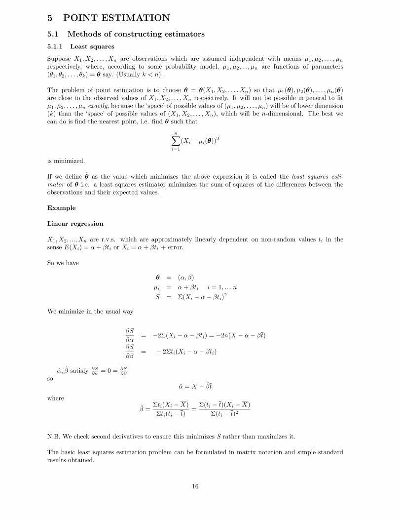
5.1.1 Least squares

Suppose X1,X2, . . . ,Xn are observations which are assumed independent with means µ1, µ2, . . . , µn

respectively, where, according to some probability model, µ1, µ2, ..., µn are functions of parameters(θ1, θ2, . . . , θk) = θ say. (Usually k < n).

The problem of point estimation is to choose θ = θ(X1,X2, . . . ,Xn) so that µ1(θ), µ2(θ), . . . , µn(θ)are close to the observed values of X1,X2, . . . ,Xn respectively. It will not be possible in general to fitµ1, µ2, . . . , µn exactly, because the ‘space’ of possible values of (µ1, µ2, . . . , µn) will be of lower dimension(k) than the ‘space’ of possible values of (X1,X2, . . . ,Xn), which will be n-dimensional. The best wecan do is find the nearest point, i.e. find θ such that

n∑

i=1

(Xi − µi(θ))2

is minimized.

If we define θ as the value which minimizes the above expression it is called the least squares esti-mator of θ i.e. a least squares estimator minimizes the sum of squares of the differences between theobservations and their expected values.

Example

Linear regression

X1,X2, ...,Xn are r.v.s. which are approximately linearly dependent on non-random values ti in thesense E(Xi) = α + βti or Xi = α + βti + error.

So we have

θ = (α, β)

µi = α + βti i = 1, ..., n

S = Σ(Xi − α − βti)2

We minimize in the usual way

∂S

∂α= −2Σ(Xi − α − βti) = −2n(X − α − βt)

∂S

∂β= − 2Σti(Xi − α − βti)

α, β satisfy ∂S∂α = 0 = ∂S

∂βso

α = X − βt

where

β =Σti(Xi − X)

Σti(ti − t)=

Σ(ti − t)(Xi − X)

Σ(ti − t)2

N.B. We check second derivatives to ensure this minimizes S rather than maximizes it.

The basic least squares estimation problem can be formulated in matrix notation and simple standardresults obtained.

16

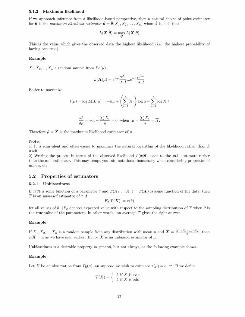
5.1.2 Maximum likelihood

If we approach inference from a likelihood-based perspective, then a natural choice of point estimatorfor θ is the maximum likelihood estimator θ = θ(X1,X2, . . . ,Xn) where θ is such that

L(X|θ) = maxθ

L(X|θ)

This is the value which gives the observed data the highest likelihood (i.e. the highest probability ofhaving occurred).

Example

X1,X2, ...,Xn a random sample from Po(µ).

L(X|µ) = e−µ µX1

X1!...e−µ µXn

Xn!

Easier to maximize

ℓ(µ) = log L(X|µ) = −nµ +

(

n∑

i=1

Xi

)

log µ −n∑

i=1

log Xi!

dℓ

dµ= −n +

∑

Xi

µ= 0 when µ =

∑

Xi

n= X.

Therefore µ = X is the maximum likelihood estimator of µ.

Note:1) It is equivalent and often easier to maximize the natural logarithm of the likelihood rather than Litself.2) Writing the process in terms of the observed likelihood L(x|θ) leads to the m.l. estimate ratherthan the m.l. estimator. This may tempt you into notational inaccuracy when considering properties ofm.l.e’s, etc.

5.2 Properties of estimators

5.2.1 Unbiasedness

If τ(θ) is some function of a parameter θ and T (X1, ...,Xn) = T (X) is some function of the data, thenT is an unbiased estimator of τ if

Eθ[T (X)] = τ(θ)

for all values of θ. [Eθ denotes expected value with respect to the sampling distribution of T when θ isthe true value of the parameter]. In other words, ‘on average’ T gives the right answer.

Example

If X1,X2, ...,Xn is a random sample from any distribution with mean µ and X = X1+X2+...+Xn

n , then

EX = µ as we have seen earlier. Hence X is an unbiased estimator of µ.

Unbiasedness is a desirable property in general, but not always, as the following example shows.

Example

Let X be an observation from P0(µ), an suppose we wish to estimate τ(µ) = e−2µ. If we define

T (X) =

1 if X is even-1 if X is odd

17

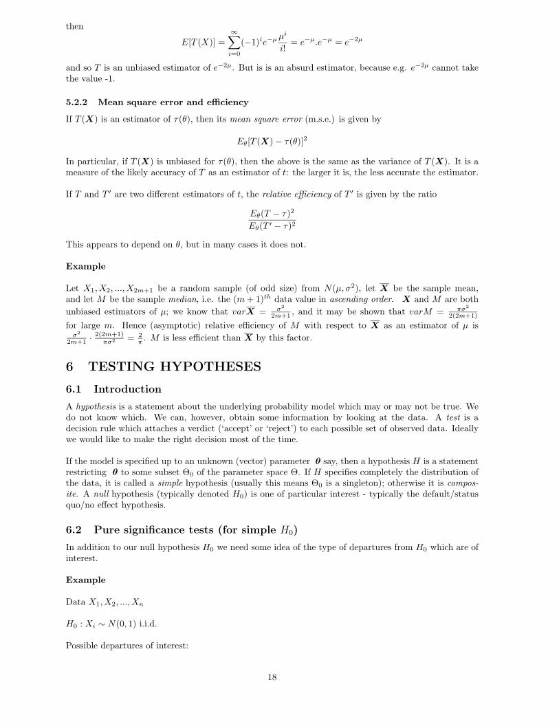
then

E[T (X)] =

∞∑

i=0

(−1)ie−µ µi

i!= e−µ.e−µ = e−2µ

and so T is an unbiased estimator of e−2µ. But is is an absurd estimator, because e.g. e−2µ cannot takethe value -1.

5.2.2 Mean square error and efficiency

If T (X) is an estimator of τ(θ), then its mean square error (m.s.e.) is given by

Eθ[T (X) − τ(θ)]2

In particular, if T (X) is unbiased for τ(θ), then the above is the same as the variance of T (X). It is ameasure of the likely accuracy of T as an estimator of t: the larger it is, the less accurate the estimator.

If T and T ′ are two different estimators of t, the relative efficiency of T ′ is given by the ratio

Eθ(T − τ)2

Eθ(T ′ − τ)2

This appears to depend on θ, but in many cases it does not.

Example

Let X1,X2, ...,X2m+1 be a random sample (of odd size) from N(µ, σ2), let X be the sample mean,and let M be the sample median, i.e. the (m + 1)th data value in ascending order. X and M are both

unbiased estimators of µ; we know that varX = σ2

2m+1 , and it may be shown that varM = πσ2

2(2m+1)

for large m. Hence (asymptotic) relative efficiency of M with respect to X as an estimator of µ isσ2

2m+1 · 2(2m+1)πσ2 = 2

π . M is less efficient than X by this factor.

6 TESTING HYPOTHESES

6.1 Introduction

A hypothesis is a statement about the underlying probability model which may or may not be true. Wedo not know which. We can, however, obtain some information by looking at the data. A test is adecision rule which attaches a verdict (‘accept’ or ‘reject’) to each possible set of observed data. Ideallywe would like to make the right decision most of the time.

If the model is specified up to an unknown (vector) parameter θ say, then a hypothesis H is a statementrestricting θ to some subset Θ0 of the parameter space Θ. If H specifies completely the distribution ofthe data, it is called a simple hypothesis (usually this means Θ0 is a singleton); otherwise it is compos-ite. A null hypothesis (typically denoted H0) is one of particular interest - typically the default/statusquo/no effect hypothesis.

6.2 Pure significance tests (for simple H0)

In addition to our null hypothesis H0 we need some idea of the type of departures from H0 which are ofinterest.

Example

Data X1,X2, ...,Xn

H0 : Xi ∼ N(0, 1) i.i.d.

Possible departures of interest:

18

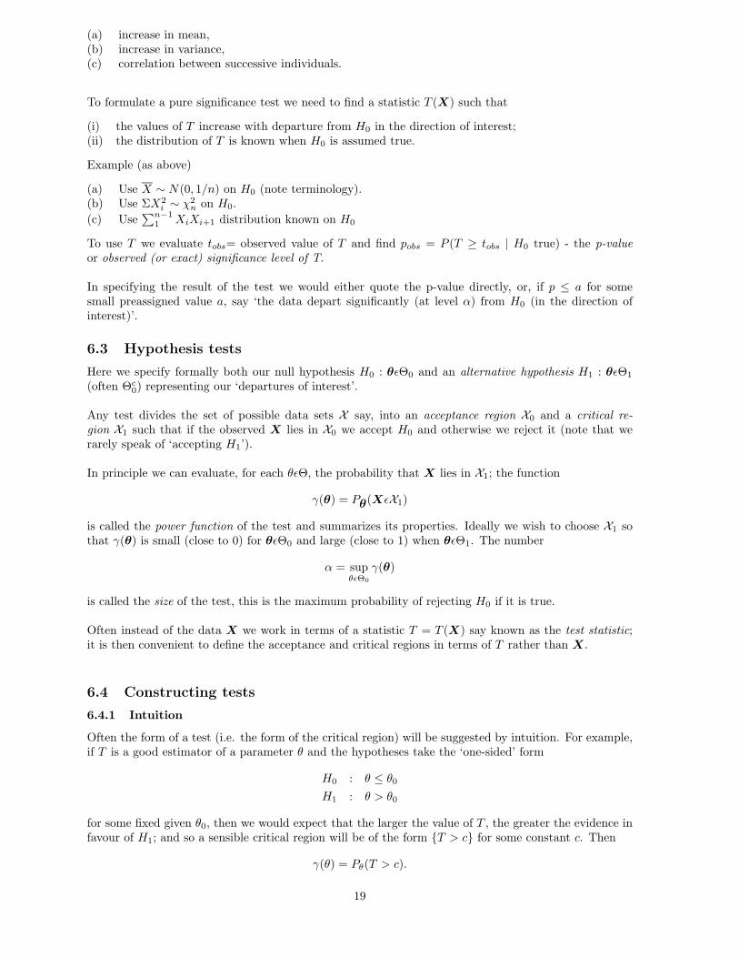
(a) increase in mean,(b) increase in variance,(c) correlation between successive individuals.

To formulate a pure significance test we need to find a statistic T (X) such that

(i) the values of T increase with departure from H0 in the direction of interest;(ii) the distribution of T is known when H0 is assumed true.

Example (as above)

(a) Use X ∼ N(0, 1/n) on H0 (note terminology).(b) Use ΣX2

i ∼ χ2n on H0.

(c) Use∑n−1

1 XiXi+1 distribution known on H0

To use T we evaluate tobs= observed value of T and find pobs = P (T ≥ tobs | H0 true) - the p-valueor observed (or exact) significance level of T.

In specifying the result of the test we would either quote the p-value directly, or, if p ≤ a for somesmall preassigned value a, say ‘the data depart significantly (at level α) from H0 (in the direction ofinterest)’.

6.3 Hypothesis tests

Here we specify formally both our null hypothesis H0 : θǫΘ0 and an alternative hypothesis H1 : θǫΘ1

(often Θc0) representing our ‘departures of interest’.

Any test divides the set of possible data sets X say, into an acceptance region X0 and a critical re-gion X1 such that if the observed X lies in X0 we accept H0 and otherwise we reject it (note that werarely speak of ‘accepting H1’).

In principle we can evaluate, for each θǫΘ, the probability that X lies in X1; the function

γ(θ) = Pθ(XǫX1)

is called the power function of the test and summarizes its properties. Ideally we wish to choose X1 sothat γ(θ) is small (close to 0) for θǫΘ0 and large (close to 1) when θǫΘ1. The number

α = supθǫΘ0

γ(θ)

is called the size of the test, this is the maximum probability of rejecting H0 if it is true.

Often instead of the data X we work in terms of a statistic T = T (X) say known as the test statistic;it is then convenient to define the acceptance and critical regions in terms of T rather than X.

6.4 Constructing tests

6.4.1 Intuition

Often the form of a test (i.e. the form of the critical region) will be suggested by intuition. For example,if T is a good estimator of a parameter θ and the hypotheses take the ‘one-sided’ form

H0 : θ ≤ θ0

H1 : θ > θ0

for some fixed given θ0, then we would expect that the larger the value of T , the greater the evidence infavour of H1; and so a sensible critical region will be of the form T > c for some constant c. Then

γ(θ) = Pθ(T > c).

19

To choose c: as c increases, γ(θ) decreases for all values of θ; for θ ∈ Θ0 this is a good thing, whereas forθ ∈ Θ1 it is a bad thing. So we must choose c so as to strike a balance. Often this is done by prescribingthe value of α (e.g. 0.05). This is sufficient to determine c. Often tables of critical values of the teststatistic for specified α are produced.

Example

X1,X2, ...,Xn a sample from N(µ, 1).

H0 : µ ≤ 0

H1 : µ > 0

Use X as test statistic; critical region will be of the form

X > c

.

γ(µ) = Pµ(X > c) = 1 − Φ(c − µ

1/√

n)

= Φ(√

n(µ − c)).

This has its maximum value in H0 when µ = 0; so if α is prescribed we must choose c such thatΦ(−c

√n) = α.

This is easily solved for c (using tables).

Example (as above)

If n = 100, α = 0.05Φ(−10c) = 0.05c = −1

10 Φ−1(0.05)Neave table 2.3(b) gives c = −1

10 (−1.6449) = 0.16449.So the test is ‘reject H0 : µ ≤ 0 at the 5% level if x > 0.16449’

6.4.2 Neyman-Pearson approach

This form is most easily introduced in the (not very practically useful) case of choosing between twosimple hypotheses H0 : θ = θ0 v H1 : θ = θ1 (it can be extended to composite hypotheses).

We consider the probabilities of making the two types of error that can occur in any test

α = P (type I error) = P (reject H0 | H0 true) = γ(θ0) as beforeβ = P (type II error) =P (do not reject H0 | H1 true) = 1 − γ(θ1).

Again, ideally we would like both α and β small, but simultaneous reduction is usually impossibleso we compromise by fixing α at an acceptably low level and then minimizing β (for this fixed α).

The Neyman-Pearson lemma tells us that the test with

X1 =

X :L(X|θ0)

L(X|θ1)< c

where c is s.t. P (XǫX1 | θ0) = α will minimize β = P (XǫX0 | θ1), i.e. it is the most powerful test oflevel α.

Typically the form of the test simplifies and we can work with a particular test statistic T and de-termine probabilities from its sampling distribution.

Example

X1,X2, ...,Xn a sample from N(µ, σ2), σ2 known.

H0 : µ = µ0 v H1 : µ = µ1 with µ1 > µ0 say.

20

Intuition suggests a test with critical region X > c and this is indeed the most powerful test:

L(X|µ) =1

(2π)n/2(σ2)n/2exp

−1

2

n∑

i=1

(Xi − µ)2

σ2

.

So the N-P lemma says the best test has critical region given by X’s for which

exp− 1

2σ2

[

∑

(Xi − µ0)2 −

∑

(Xi − µ1)2]

< c

i.e. − 12σ2 [

∑

X2i − 2µ0

∑

Xi + µ20 −

∑

X2i + 2µ1

∑

Xi − µ21] < c′

i.e.∑

Xi(µ1 − µ0) > c′′ (take care over direction of inequality)

i.e. X > c′′′ = k say recalling µ1 − µ0 > 0.

k is determined by the requirement

P (XǫX1 | µ = µ0) = α

i.e. P (X > k | µ = µ0) = α

Sampling distribution of X on H0 is N(µ0, σ2/n)

Therefore P (X > k | µ = µ0) = P(

X−µ0

σ/√

n > k−µ0

σ/√

n

)

= α

i.e. k = µ0 + σ√nΦ−1(1 − α) evaluated using Neave 2.3(b).

6.4.3 The likelihood ratio procedure

This is a method of suggesting a form of test which in principle always works. It gives the same re-sult as the Neyman-Pearson test in the simple v. simple case (despite the difference in the denominator)and extends easily to more general situations. There is also a useful asymptotic result about it (see later).

The test is defined by considering the ratio

supθ∈Θ0

L(X|θ)

supθ∈Θ

L(X|θ)= Λ.

This ratio is always < 1 since the supremum in the denominator is over a larger set. The further Λis from 1, the greater the evidence against H0. Hence a form of critical region which suggests itself isΛ < c.

Example

X1,X2, ...,Xn a sample from N(µ, σ2) with both µ and σ2 unknown.

H0 : µ = µ0

a ‘two-sided’ test.H1 : µ 6= µ0

Here Θ0 =

(µ, σ2); µ = µ0, σ2 > 0

and Θ =

(µ, σ2); σ2 > 0

.

21

The likelihood is

L(X|θ) =1

(2π)n/2(σ2)n/2exp

[

−1

2

n∑

i=1

(Xi − µ)2

σ2

]

.

This is maximized in Θ0 by putting µ = µ0 and σ2 = 1n

∑ni=1(Xi−µ0)

2 (check by differentiating!), giving

maxθ∈Θ0

L(X|θ) =nn/2 e−n/2

(2π)n/2 [∑

(Xi − µ0)2]n/2

,

It is maximized in Θ by putting µ = X and σ2 = 1n

∑ni=1(Xi − X)2,

giving

maxθ∈Θ

L(X|θ) =nn/2 e−n/2

(2π)n/2[∑

(Xi − X)2]n/2

.

Hence the critical region takes the form

(∑

(Xi − X)2∑

(Xi − µ0)2

)n/2

< c.

Since∑

(Xi − µ0)2 =

∑

(Xi − X)2 + n(X − µ0)2, this is equivalent to

(X − µ0)2

∑

(Xi − X)2> c′

orX−µ0

S> c′′

where S2 is the sample variance.

The statistic T =√

n(X−µ0)S is called the one-sample t statistic.

Its sampling distribution if µ = µ0 does not depend upon σ2, and is known as the t distribution withn − 1 degrees of freedom. So a test of given size may be constructed using tables of critical values forthis distribution (Neave 3.1).

The form of test suggested by the likelihood ratio procedure often simplifies, as above, but the sam-pling distribution of the simplified test statistic must be derived by ‘ad hoc’ methods - and even thisis not always possible. It is, therefore, useful to have a general asymptotic result which works underreasonable regularity conditions as the sample size n → ∞; this is that if H0 is true −2 log Λ is asymptoti-cally χ2

ν where ν, the number of degrees of freedom, is the difference in dimensionality between Θ0 and Θ.

Example

If (X11, ...,X1n), (X21, ...,X2n), ..., (Xk1, ...,Xkn) are samples from N(µ1, σ21), ..., N(µk, σ2

k) respectivelywhere µ1, σ

21 , ..., µk, σ2

k are all unknown, and we wish to test H0 : σ21 = σ2

2 = ... = σ2k, then the unre-

stricted parameter space Θ is 2k-dimensional whereas Θ0 is (k+1)-dimensional, since H0 imposes (k−1)linear constraints. Hence −2logΛ ∼ X2

k−1 asymptotically.

7 INTERVAL ESTIMATION

In a point estimation we aim to produce a single ‘best guess’ at a parameter value θ. Here we provide aregion (usually an interval) in which θ ‘probably lies’.

Construction is via inversion of a probability statement concerning the data, so if T is a statistic derivedfrom the data we find, by examining the sampling distribution of T , a region A(θ) such that

P (TǫA(θ)) = 1 − α

22

for some suitable small α, and invert this to identify the region C(T ) = [θ : TǫA(θ)] which then satisfies

P (θǫC(T )) = 1 − α.

In other words, the ‘random region’ C(T ) ‘covers’ the true parameter value θ with probability 1 − α.C(T ) is usually an interval, called a confidence interval for θ. The confidence level is usually expressedas a percentage: 100(1-α) % (e.g. α = 0.05 gives a 95% confidence interval).

Example

X1,X2, ...,Xn a random sample from N(µ, σ2) with µ unknown, σ2 known. T = X with

X ∼ N(µ, σ2/n).

ThusX − µ

σ/√

n∼ N(0, 1)

P

(

−z1−α/2 ≤ X − µ

σ/√

n≤ z1−α/2

)

= 1 − α (∗)

where z1−α/2 solves Φ(z1−α/2) = 1 − α/2 (from tables).

Thus

P

(

µ − z1−α/2.σ√n≤ X ≤ µ + z1−α/2.

σ√n

)

= 1 − α (∗∗)

so

A(µ) =

(

µ − z1−α/2.σ√n

, µ + z1−α/2.σ√n

)

Inverting (∗∗)P

[

X − z1−α/2.σ√n≤ µ ≤ X + z1−α/2.

σ√n

]

= 1 − α

i.e.

C(T ) =

(

X − z1−α/2.σ√n

,X + z1−α/2.σ√n

)

.

Note: we have chosen the z1−α/2 in (∗) symmetrically; we could have chosen any z values giving overallprobability level 1 − α.In general if an estimator θ is asymptotically normally distributed with mean equal to the true value ofthe parameter θ, then an approximate 100(1 − α)% confidence interval is given by

(

θ − z1−α/2σθ, θ + z1−α/2σθ

)

where σθ, the standard deviation of the sampling distribution of θ, is called the standard error. Thismay itself have to be estimated from the data.

In fact there is a duality with hypothesis testing in that possible parameter values which would notbe rejected in a size α test are those which constitute the 100(1−α)% confidence interval. This gives usa direct means of establishing A(θ):

Let A(θ0) denote the acceptance region for a standard test of size α of H0 : θ = θ0 (simple) againstH1 : θ 6= θ0 using a test statistic T .

Then we havePθ0

(TǫA(θ0)) = 1 − α for all θ0.

Defining C(T ) as above, this may be written

Pθ(θǫC(T )) = 1 − α.

So C(T ) is a confidence interval for θ.

23

8 BAYESIAN METHODS AND DECISION THEORY

8.1 Bayesian Methods

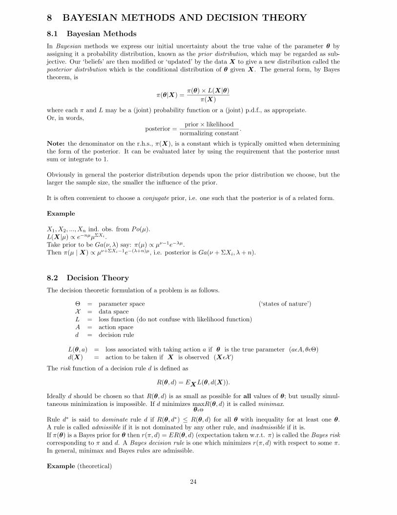
In Bayesian methods we express our initial uncertainty about the true value of the parameter θ byassigning it a probability distribution, known as the prior distribution, which may be regarded as sub-jective. Our ‘beliefs’ are then modified or ‘updated’ by the data X to give a new distribution called theposterior distribution which is the conditional distribution of θ given X. The general form, by Bayestheorem, is

π(θ|X) =π(θ) × L(X|θ)

π(X)

where each π and L may be a (joint) probability function or a (joint) p.d.f., as appropriate.Or, in words,

posterior =prior × likelihood

normalizing constant.

Note: the denominator on the r.h.s., π(X), is a constant which is typically omitted when determiningthe form of the posterior. It can be evaluated later by using the requirement that the posterior mustsum or integrate to 1.

Obviously in general the posterior distribution depends upon the prior distribution we choose, but thelarger the sample size, the smaller the influence of the prior.

It is often convenient to choose a conjugate prior, i.e. one such that the posterior is of a related form.

Example

X1,X2, ...,Xn ind. obs. from Po(µ).L(X|µ) ∝ e−nµµΣXi .Take prior to be Ga(ν, λ) say: π(µ) ∝ µν−1e−λµ.Then π(µ | X) ∝ µν+ΣXi−1e−(λ+n)µ, i.e. posterior is Ga(ν + ΣXi, λ + n).

8.2 Decision Theory

The decision theoretic formulation of a problem is as follows.

Θ = parameter space (‘states of nature’)X = data spaceL = loss function (do not confuse with likelihood function)A = action spaced = decision rule

L(θ, a) = loss associated with taking action a if θ is the true parameter (aǫA, θǫΘ)d(X) = action to be taken if X is observed (XǫX )

The risk function of a decision rule d is defined as

R(θ, d) = EXL(θ, d(X)).

Ideally d should be chosen so that R(θ, d) is as small as possible for all values of θ; but usually simul-taneous minimization is impossible. If d minimizes max

θǫΘR(θ, d) it is called minimax.

Rule d∗ is said to dominate rule d if R(θ, d∗) ≤ R(θ, d) for all θ with inequality for at least one θ.A rule is called admissible if it is not dominated by any other rule, and inadmissible if it is.If π(θ) is a Bayes prior for θ then r(π, d) = ER(θ, d) (expectation taken w.r.t. π) is called the Bayes riskcorresponding to π and d. A Bayes decision rule is one which minimizes r(π, d) with respect to some π.In general, minimax and Bayes rules are admissible.

Example (theoretical)

24

A = Θ, i.e. ‘action’ = ‘point estimate of parameter’.d(X) = θ(X) = ‘estimator’.

L(θ, θ(X)) = (θ(X) − θ)2 (quadratic loss).

R(θ, θ) = Eθ(θ − θ)2 = mean square error.

Let X = an observation from P0(µ). Then

R(µ, µ) =∞∑

i=1

(µ(i) − µ)2e−µµi/i!

Suppose π(µ) = λν

Γ(ν)µν−1e−λµ (Gamma prior).

Then

r(π, µ) =

∞∑

i=0

λν

Γ(ν)

∫ ∞

0

(µ(i) − µ)2e−µ µi

i!µν−1e−µdµ

=∞∑

i=1

λν

Γ(ν)i!

Γ(ν + i)

(λ + 1)ν+iµ(i)2 − 2

Γ(ν + i + 1)

(λ + 1)ν+i+1µ(i) +

Γ(ν + i + 2)

(λ + 1)ν+i+2

this is minimized for each i by taking

µ(i) =Γ(ν + i + 1)

(λ + 1)ν+i+1

(λ + 1)ν+i

Γ(ν + 1)=

ν + i

λ + 1.

Hence µ(X) = ν+Xλ+1 is the Bayes estimator.

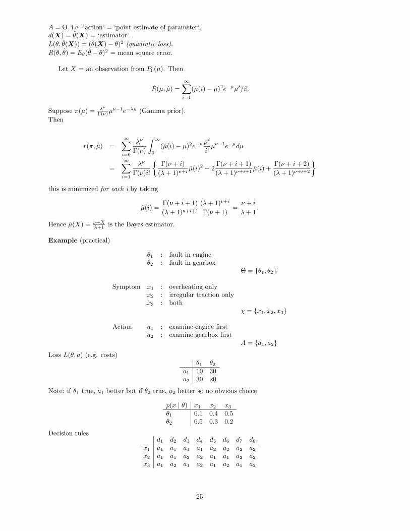
Example (practical)

θ1 : fault in engineθ2 : fault in gearbox

Θ = θ1, θ2

Symptom x1 : overheating onlyx2 : irregular traction onlyx3 : both

χ = x1, x2, x3

Action a1 : examine engine firsta2 : examine gearbox first

A = a1, a2Loss L(θ, a) (e.g. costs)

θ1 θ2

a1 10 30a2 30 20

Note: if θ1 true, a1 better but if θ2 true, a2 better so no obvious choice

p(x | θ) x1 x2 x3

θ1 0.1 0.4 0.5θ2 0.5 0.3 0.2

Decision rulesd1 d2 d3 d4 d5 d6 d7 d8

x1 a1 a1 a1 a1 a2 a2 a2 a2

x2 a1 a1 a2 a2 a1 a1 a2 a2

x3 a1 a2 a1 a2 a1 a2 a1 a2

25

R(θ, d)d1 d2 d3 d4 d5 d6 d7 d8

θ1 10 20 18 28 12 22 20 30θ2 30 28 27 25 25 23 22 20

For θ1, best d is d1

For θ2, best d is d8

Note that simultaneous minimization is usually not possible.

(i) Minimax

Choose d from mind maxΘR(θ, d),

i.e. d7 here.

(ii) Admissible set

Note that d2 always worse than d5.

Similarly never use d2, d3, d4, d6 they are inadmissibleThis leaves as admissible set

d1 d5 d7 d8

θ1 10 12 20 30θ2 30 25 22 22

(iii) Bayesian

Supposeπ(θ1) = 0.4π(θ2) = 0.6

Bayes risk r(π, d) = EθR(θ, d) = ΣΘR(θ, d)π(θ)

d1 d5 d7 d8

r(π, d) 22 19.8 21.2 24

So d5 is the Bayes rule.

26