Embed Size (px)
Citation preview

TEM
F) Large Scale 3D Wakefield Si l i i h PBCI
her F
elde
r ( Simulations with PBCI
mag
netis
ch S. Schnepp, W. Ackermann, E. Arevalo,E. Gjonaj, and T. Weiland
al.
orie
Ele
ktro
"Wake Fest 07 - ILC wakefield workshop at SLAC”11 13 D b 2007
Schn
epp
et a
tut f
ür T
heo 11-13 December 2007
Technische Universität Darmstadt, Fachbereich Elektrotechnik und InformationstechnikSchloßgartenstr. 8 , 64289 Darmstadt, Germany - URL: www.TEMF.de
Technische Universität Darmstadt, Fachbereich Elektrotechnik und InformationstechnikSchloßgartenstr. 8 , 64289 Darmstadt, Germany - URL: www.TEMF.de
S. S
Inst
i
Outline
•• IntroductionIntroduction
TEM
F)
•• IntroductionIntroduction
•• NumericalNumerical MethodMethod
her F
elde
r (
•• Parallelization StrategyParallelization Strategy
mag
netis
ch •• Modal Termination of Beam PipesModal Termination of Beam Pipes
•• PBCI Simulation ExamplesPBCI Simulation Examples
al.
orie
Ele
ktro
PBCI Simulation ExamplesPBCI Simulation Examples
Schn
epp
et a
tut f
ür T
heo
1
S. S
Inst
i
Introduction
1 A new generation of LINACs with ultra short electron bunches
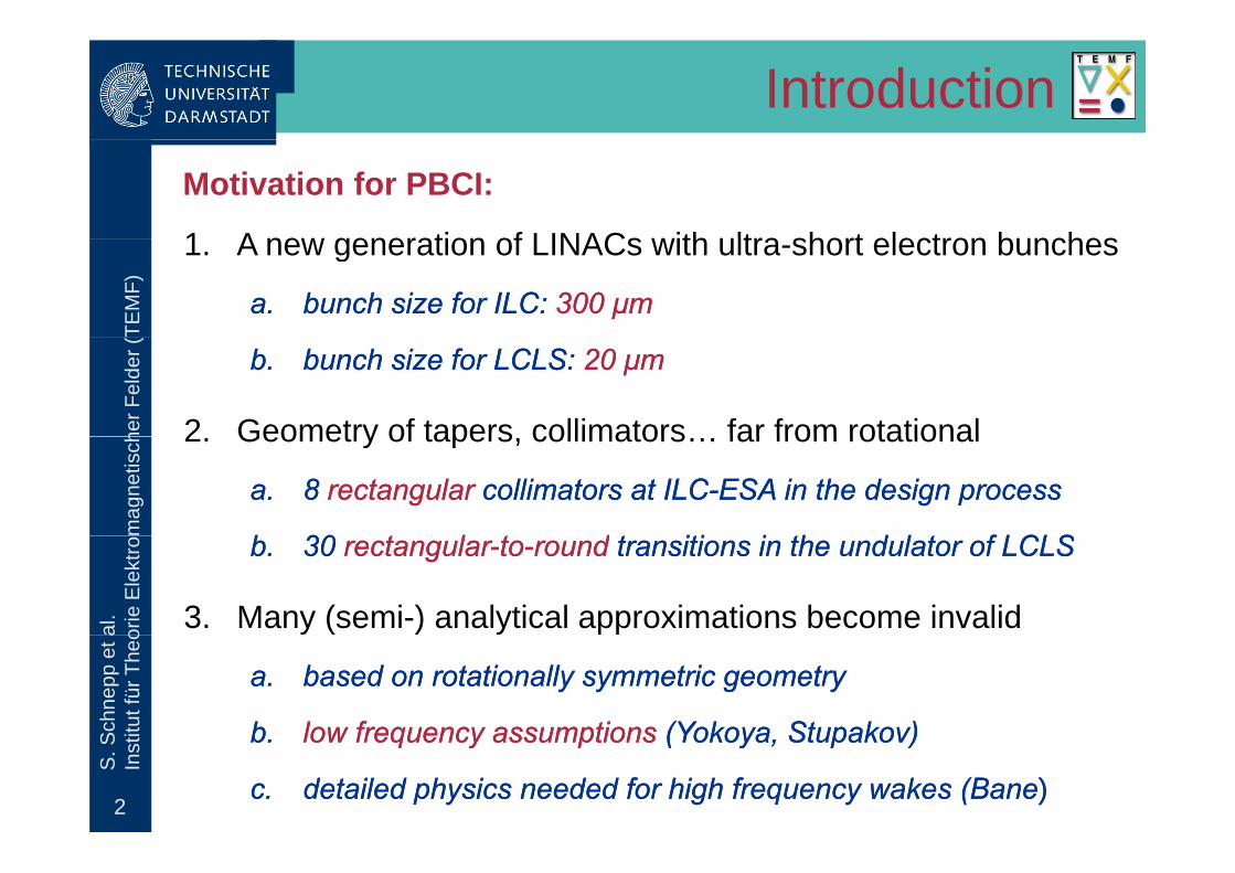
Motivation for PBCI:TE
MF)
1. A new generation of LINACs with ultra-short electron bunches
a.a. bunch size for ILC: bunch size for ILC: 300 300 μμmm
her F
elde
r ( b.b. bunch size for LCLbunch size for LCLSS: : 20 20 μμmm
2 Geometry of tapers collimators far from rotational
mag
netis
ch 2. Geometry of tapers, collimators… far from rotational
a.a. 8 8 rectangularrectangular collimators at collimators at ILCILC--ESA in the design processESA in the design process
bb 3030 t lt l tt dd t iti i th d l t f LCLt iti i th d l t f LCLSS
al.
orie
Ele
ktro b.b. 30 30 rectangularrectangular--toto--roundround transitions in the undulator of LCLtransitions in the undulator of LCLSS
3. Many (semi-) analytical approximations become invalid
Schn
epp
et a
tut f
ür T
heo
a.a. based on rotationally symmetric geometrybased on rotationally symmetric geometry
bb low frequency assumptionslow frequency assumptions (Yokoya Stupakov)(Yokoya Stupakov)
2
S. S
Inst
i b.b. low frequency assumptionslow frequency assumptions (Yokoya, Stupakov)(Yokoya, Stupakov)
c.c. detailed physics needed for high frequency wakes (Banedetailed physics needed for high frequency wakes (Bane))
Introduction
38 1mm
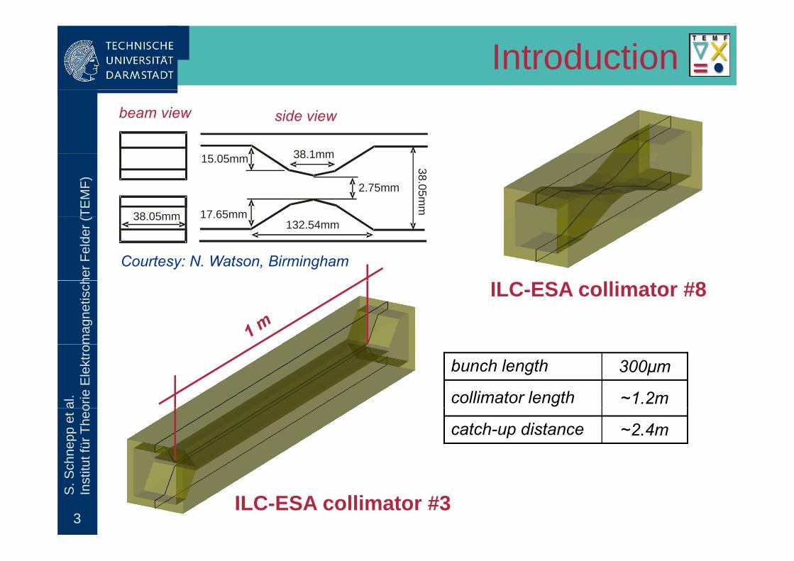
beam view side view
TEM
F)
38.1mm15.05mm
2.75mm
17 65mm38 05mm
38.05mm
her F
elde
r ( 132.54mm17.65mm38.05mm
Courtesy: N. Watson, Birmingham
mag
netis
ch ILC-ESA collimator #8
al.
orie
Ele
ktro
bunch length 300μm
collimator length ~1.2m
Schn
epp
et a
tut f
ür T
heo
catch-up distance ~2.4m
3
S. S
Inst
i
ILC-ESA collimator #3
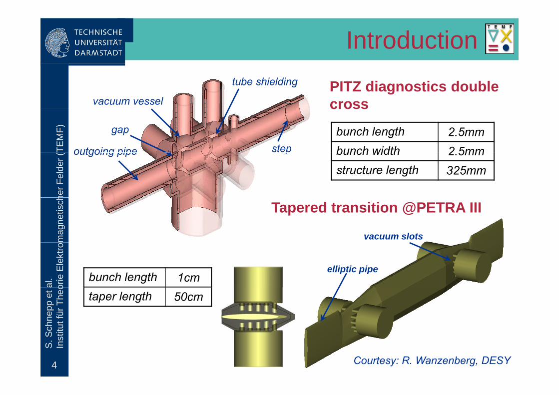
Introductiontube shielding
vacuum vesselPITZ diagnostics double cross
TEM
F)
outgoing pipe step
gap
cross
bunch length 2.5mmbunch width 2 5mm
her F
elde
r (
outgoing pipe p bunch width 2.5mmstructure length 325mm
mag
netis
ch Tapered transition @PETRA III
vacuum slots
al.
orie
Ele
ktro
bunch length 1cmelliptic pipe
Schn
epp
et a
tut f
ür T
heo
taper length 50cm
4
S. S
Inst
i
Courtesy: R. Wanzenberg, DESY
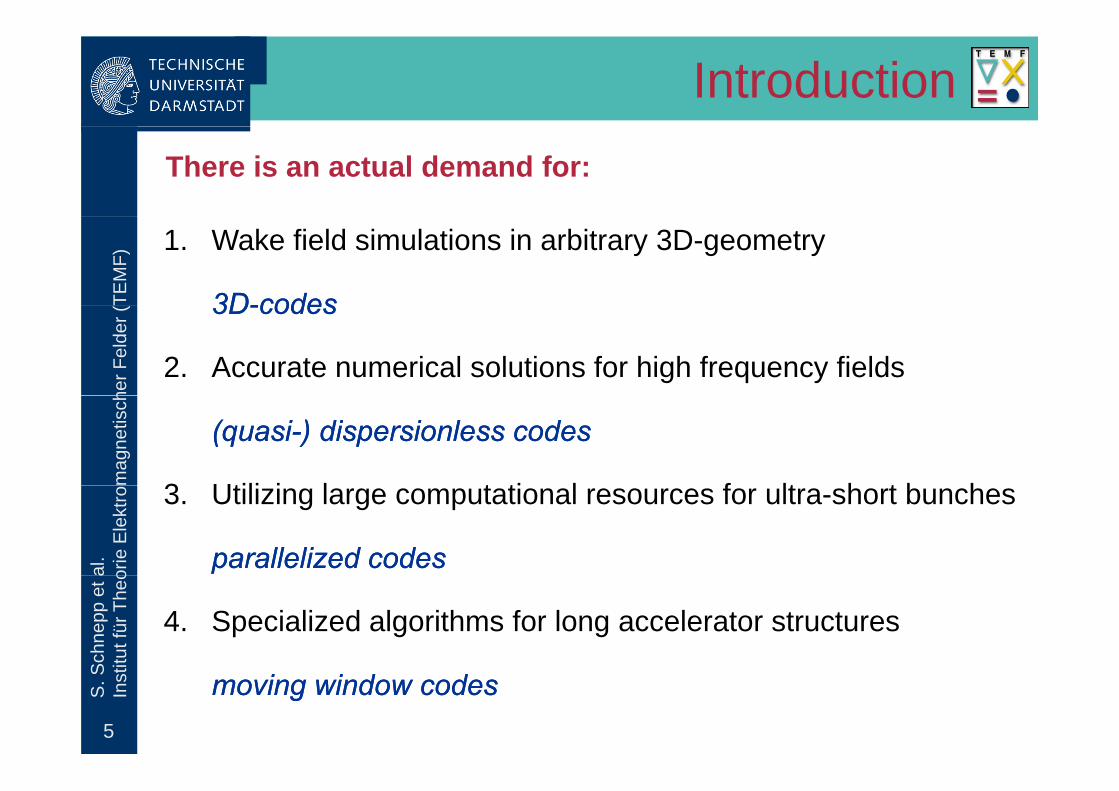
IntroductionThere is an actual demand for:
TEM
F)
1. Wake field simulations in arbitrary 3D-geometry
3D3D--codescodes
her F
elde
r ( 3D3D--codescodes
2. Accurate numerical solutions for high frequency fields
mag
netis
ch
(quasi(quasi--) dispersionless codes) dispersionless codes
3 Utili i l t ti l f lt h t b h
al.
orie
Ele
ktro 3. Utilizing large computational resources for ultra-short bunches
parallelized codesparallelized codes
Schn
epp
et a
tut f
ür T
heo
4. Specialized algorithms for long accelerator structures
5
S. S
Inst
i
moving window codesmoving window codes
Introduction
Di i N di i P ll li d M i i d
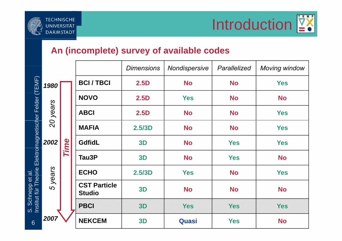
An (incomplete) survey of available codesTE
MF)
Dimensions Nondispersive Parallelized Moving window
BCI / TBCI 2.5D No No Yes1980
her F
elde
r ( NOVO 2.5D Yes No No
ABCI 2.5D No No Yes
0 ye
ars
mag
netis
ch
MAFIA 2.5/3D No No Yes
GdfidL 3D No Yes Yesme
20
2002
al.
orie
Ele
ktro
Tau3P 3D No Yes No
ECHO 2.5/3D Yes No Yes
Tim
ars
Schn
epp
et a
tut f
ür T
heo
CST ParticleStudio 3D No No No5
yea
6
S. S
Inst
i PBCI 3D Yes Yes Yes
NEKCEM 3D Quasi Yes No2007
Outline
•• IntroductionIntroduction
TEM
F)
•• IntroductionIntroduction
•• NumericalNumerical MethodMethod
her F
elde
r (
•• Parallelization StrategyParallelization Strategy
mag
netis
ch •• Modal Termination of Beam PipesModal Termination of Beam Pipes
•• PBCI Simulation ExamplesPBCI Simulation Examples
al.
orie
Ele
ktro
PBCI Simulation ExamplesPBCI Simulation Examples
Schn
epp
et a
tut f
ür T
heo
7
S. S
Inst
i
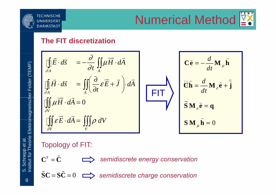
Numerical MethodThe FIT discretization
TEM
F)
A A
E ds H dAt∂
∂ μ∂
⋅ = − ⋅∫ ∫∫uur rr r
ddt μ= −Ce M h
))
her F
elde
r (
A A
H ds E J dAt∂
ε∂⎛ ⎞⋅ = + ⋅⎜ ⎟∂⎝ ⎠∫ ∫∫
∫∫
ur rr rr
FIT d
dt ε= +Ch M e j)) ))
mag
netis
ch 0V
H dA
E dA dV∂
μ
ε ρ
⋅ =∫∫
∫∫ ∫∫∫
uur r
ur r
%ε =S M e q)
)
al.
orie
Ele
ktro
V V
E dA dV∂
ε ρ⋅ =∫∫ ∫∫∫ 0μ =S M h
Schn
epp
et a
tut f
ür T
heo
T =C C% semidiscrete energy conservation
Topology of FIT:
8
S. S
Inst
i
0= =SC SC% % semidiscrete charge conservation
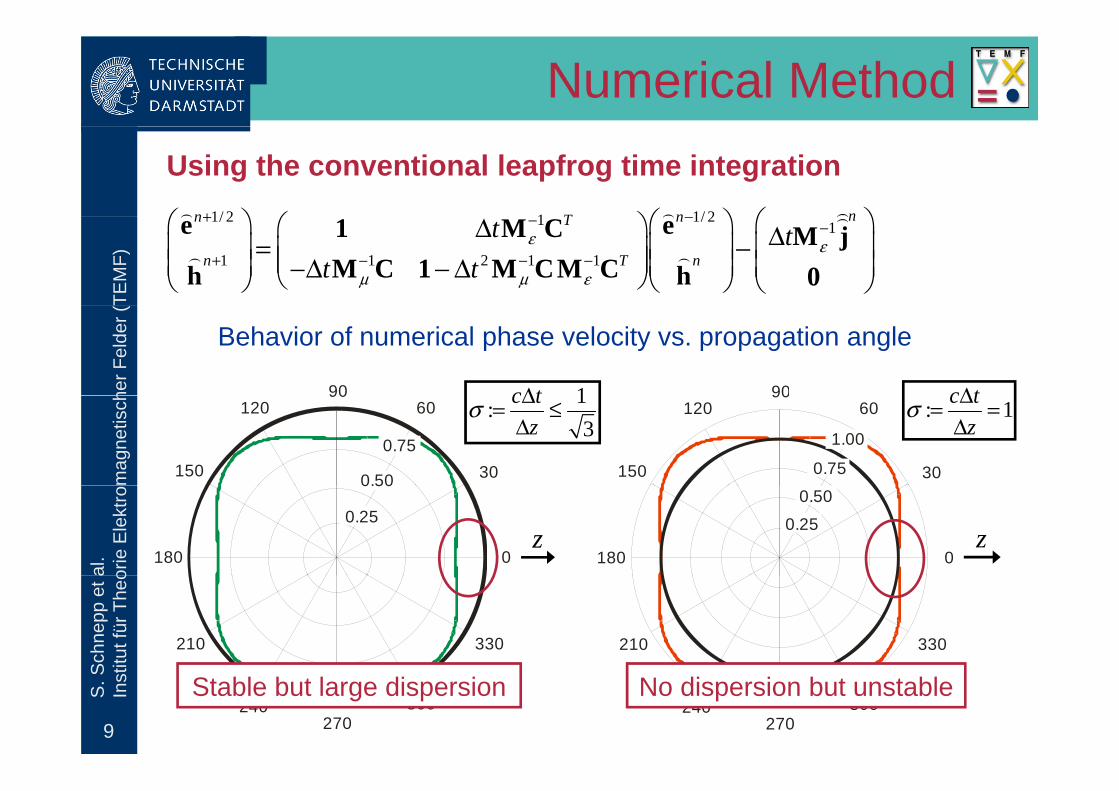
Numerical MethodUsing the conventional leapfrog time integration
1/ 2 1/ 21 nn nT+ ⎛ ⎞⎛ ⎞ ⎛ ⎞⎛ ⎞)) )
TEM
F)
1/ 2 1/ 21 1
1 1 2 1 1
nn nT
n T n
t tt t
ε ε
μ μ ε
+ −− −
+ − − −
⎛ ⎞⎛ ⎞ ⎛ ⎞⎛ ⎞Δ Δ⎜ ⎟= −⎜ ⎟ ⎜ ⎟⎜ ⎟⎜ ⎟⎜ ⎟ ⎜ ⎟ ⎜ ⎟−Δ − Δ⎝ ⎠⎝ ⎠ ⎝ ⎠ ⎝ ⎠
e e1 M C M jM C 1 M CM Ch h 0
)) ) )
) )
her F
elde
r (
9090
Behavior of numerical phase velocity vs. propagation angle
1c tΔ c tΔ
mag
netis
ch 12090
60
30150 0.75
1.00
12090
60
301500.75
0.50
1:3
c tz
σ Δ= ≤Δ
: 1c tz
σ Δ= =Δ
al.
orie
Ele
ktro
0180
0.50
0.25
0180
0.50
0.25z z
Schn
epp
et a
tut f
ür T
heo
330210330210
9
S. S
Inst
i
300270
240300270
240Stable but large dispersion No dispersion but unstable
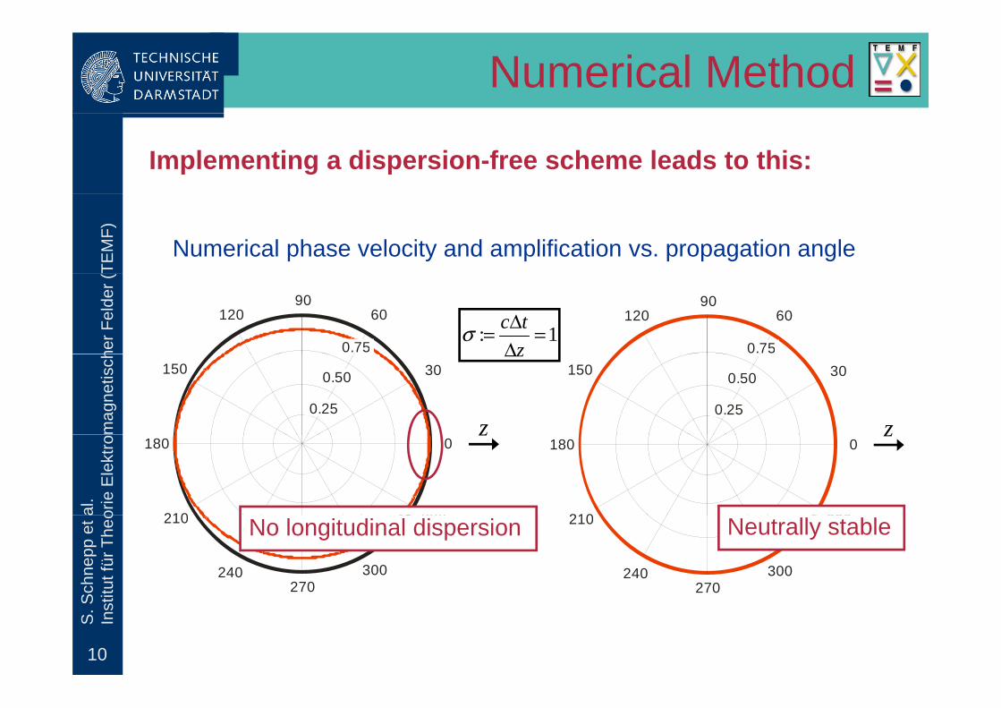
Numerical Method
Implementing a dispersion-free scheme leads to this:
TEM
F)
Numerical phase velocity and amplification vs. propagation angle
her F
elde
r (
12090
60
0.75
12090
60
0.75: 1c t
zσ Δ= =
Δ
mag
netis
ch
z
30150 0.50
0.25
30150 0.50
0.25z
zΔ
al.
orie
Ele
ktro
z0
330210
180 0
330210
180z
Schn
epp
et a
tut f
ür T
heo 330
300270
240
210 330
300270
240
210 Neutrally stableNo longitudinal dispersion
10
S. S
Inst
i
Outline
•• IntroductionIntroduction
TEM
F)
•• IntroductionIntroduction
•• NumericalNumerical MethodMethod
her F
elde
r (
•• Parallelization StrategyParallelization Strategy
mag
netis
ch •• Modal Termination of Beam PipesModal Termination of Beam Pipes
•• PBCI Simulation ExamplesPBCI Simulation Examples
al.
orie
Ele
ktro
PBCI Simulation ExamplesPBCI Simulation Examples
Schn
epp
et a
tut f
ür T
heo
11
S. S
Inst
i
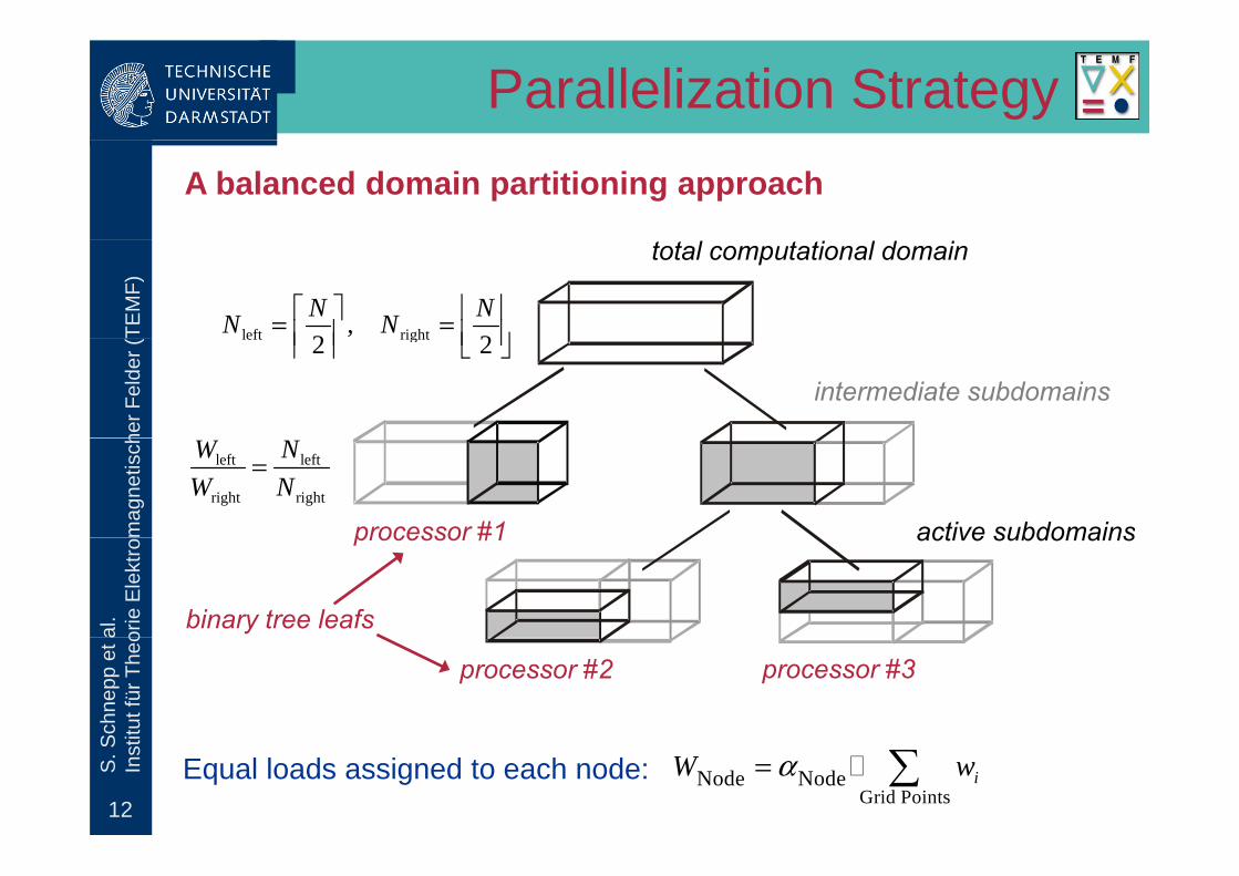
Parallelization StrategyA balanced domain partitioning approach
TEM
F)
total computational domain
left right,2 2N NN N⎡ ⎤ ⎢ ⎥= =⎢ ⎥ ⎢ ⎥⎢ ⎥ ⎣ ⎦
her F
elde
r (
intermediate subdomains
left right2 2⎢ ⎥ ⎢ ⎥⎢ ⎥ ⎣ ⎦
mag
netis
ch
active subdomains
left left
right right
W NW N
=
processor #1
al.
orie
Ele
ktro
active subdomainsprocessor #1
binary tree leafs
Schn
epp
et a
tut f
ür T
heo
processor #2 processor #3
12
S. S
Inst
i
Equal loads assigned to each node:Grid Points
Node Node iW wα= ∑
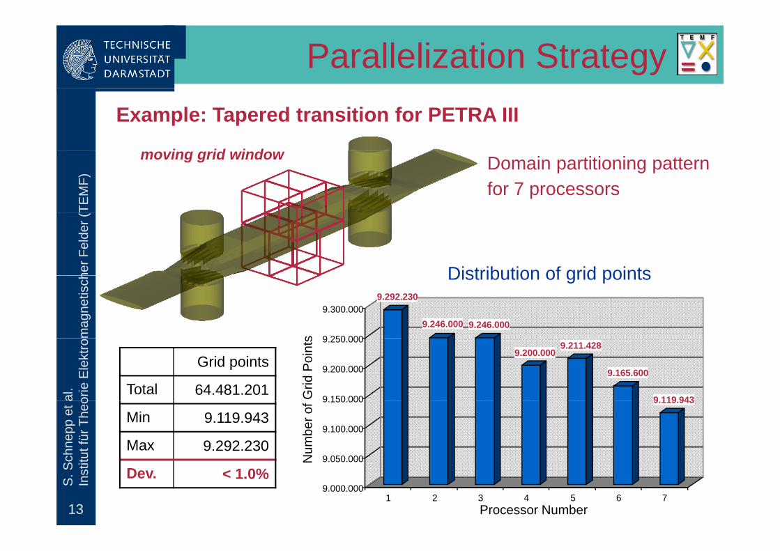
Parallelization Strategy
i id i d
Example: Tapered transition for PETRA IIITE
MF)
moving grid window Domain partitioning pattern for 7 processors
her F
elde
r (
Distribution of grid points
mag
netis
ch
9.292.230
9.246.000 9.246.0009 250 000
9.300.000s
Distribution of grid points
al.
orie
Ele
ktro 9.200.000
9.211.428
9.165.600
9 119 9439 150 000
9.200.000
9.250.000
Grid
Poi
nts
Grid points
Total 64.481.201
Schn
epp
et a
tut f
ür T
heo 9.119.943
9.050.000
9.100.000
9.150.000
Num
ber o
f
Min 9.119.943
Max 9.292.230
13
S. S
Inst
i
9.000.0001 2 3 4 5 6 7
Processor Number
Dev. < 1.0%
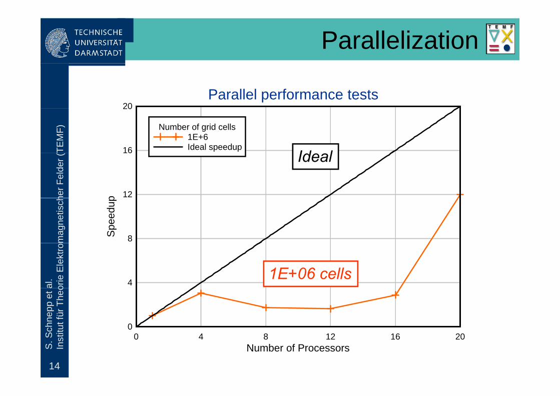
Parallelization
20Parallel performance tests
TEM
F)
16
20
Number of grid cells1E+6Ideal speedup
Id l
her F
elde
r (
p 12
16 Ideal
mag
netis
ch
Spee
dup
8
al.
orie
Ele
ktro
41E+06 cells
Schn
epp
et a
tut f
ür T
heo
0
14
S. S
Inst
i
Number of Processors0 4 8 12 16 20
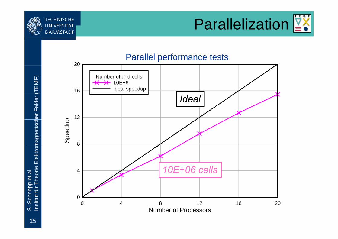
Parallelization
20Parallel performance tests
TEM
F)
16
20
Number of grid cells10E+6Ideal speedup
her F
elde
r (
p 12
16
Ideal
mag
netis
ch
Spee
dup
8
al.
orie
Ele
ktro
4 10E+06 cells
Schn
epp
et a
tut f
ür T
heo
0
15
S. S
Inst
i
Number of Processors0 4 8 12 16 20

Parallelization
20Parallel performance tests
TEM
F)
16
20
Number of grid cells50E+6Ideal speedup
her F
elde
r (
p 12
16
Ideal
mag
netis
ch
Spee
dup
8
al.
orie
Ele
ktro
4 50E+06 cells
Schn
epp
et a
tut f
ür T
heo
0
16
S. S
Inst
i
Number of Processors0 4 8 12 16 20
Parallelization
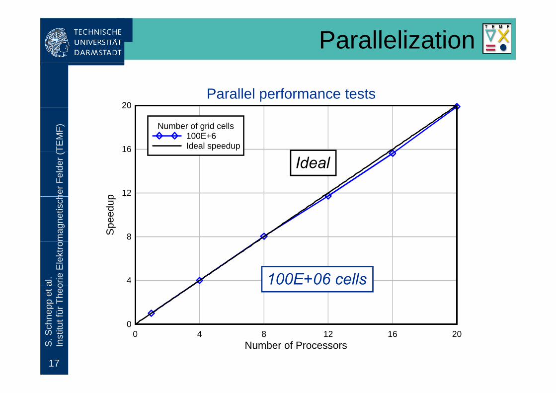
20Parallel performance tests
TEM
F)
16
20
Number of grid cells100E+6Ideal speedup
her F
elde
r (
p 12
16
Ideal
mag
netis
ch
Spee
dup
8
al.
orie
Ele
ktro
4 100E+06 cells
Schn
epp
et a
tut f
ür T
heo
0
17
S. S
Inst
i
Number of Processors0 4 8 12 16 20
Parallelization
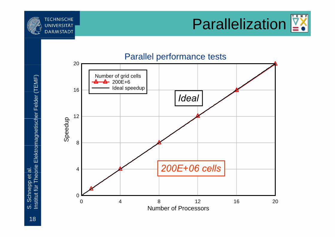
20Parallel performance tests
TEM
F)
16
20
Number of grid cells200E+6Ideal speedup
her F
elde
r (
p 12
16
Ideal
mag
netis
ch
Spee
dup
8
al.
orie
Ele
ktro
4 200E+06 cells
Schn
epp
et a
tut f
ür T
heo
0
18
S. S
Inst
i
Number of Processors0 4 8 12 16 20
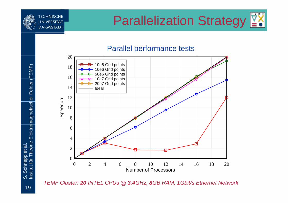
Parallelization Strategy
20Parallel performance tests
TEM
F)
16
18
2010e5 Grid points10e6 Grid points50e6 Grid points10e7 Grid points
her F
elde
r (
up
12
14
16 10e7 Grid points20e7 Grid pointsIdeal
mag
netis
ch
Spe
edu
8
10
al.
orie
Ele
ktro
2
4
6
Schn
epp
et a
tut f
ür T
heo
Number of Processors0 2 4 6 8 10 12 14 16 18 20
0
2
19
S. S
Inst
i Number of Processors
TEMF Cluster: 20 INTEL CPUs @ 3.4GHz, 8GB RAM, 1Gbit/s Ethernet Network
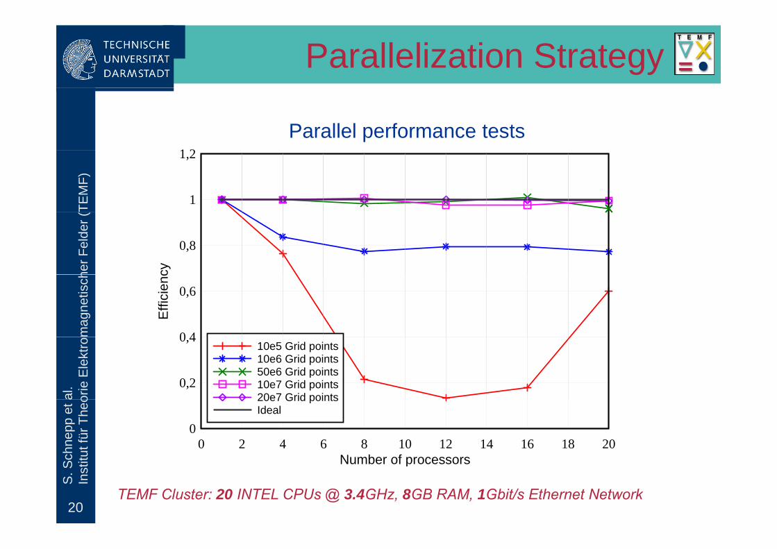
Parallelization Strategy
1 2Parallel performance tests
TEM
F)
1
1,2
her F
elde
r (
cy
0,8
mag
netis
ch
Effi
cien
c
0 4
0,6
al.
orie
Ele
ktro
0,2
0,410e5 Grid points10e6 Grid points50e6 Grid points10e7 Grid points20e7 Grid points
Schn
epp
et a
tut f
ür T
heo
Number of processors0 2 4 6 8 10 12 14 16 18 20
0
20e7 Grid pointsIdeal
20
S. S
Inst
i Number of processors
TEMF Cluster: 20 INTEL CPUs @ 3.4GHz, 8GB RAM, 1Gbit/s Ethernet Network
Outline
•• IntroductionIntroduction
TEM
F)
•• IntroductionIntroduction
•• NumericalNumerical MethodMethod
her F
elde
r (
•• Parallelization StrategyParallelization Strategy
mag
netis
ch •• Modal Termination of Beam PipesModal Termination of Beam Pipes
•• PBCI Simulation ExamplesPBCI Simulation Examples
al.
orie
Ele
ktro
PBCI Simulation ExamplesPBCI Simulation Examples
Schn
epp
et a
tut f
ür T
heo
21
S. S
Inst
i
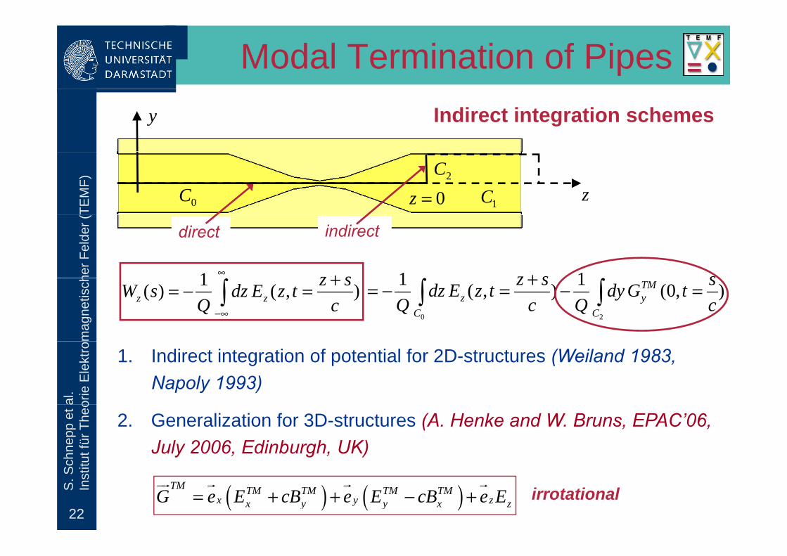
Modal Termination of Pipesy Indirect integration schemes
TEM
F)
z2C
0C 1C0z =
her F
elde
r (
1 z s∞ +
direct indirect
1 1z s s+∫ ∫
mag
netis
ch 1( ) ( , )z zz sW s dz E z t
Q c−∞
+= − =∫0 2
1 1( , ) (0, )TMz y
C C
z s sdz E z t dyG tQ c Q c
+= − = − =∫ ∫
al.
orie
Ele
ktro 1. Indirect integration of potential for 2D-structures (Weiland 1983,
Napoly 1993)
Schn
epp
et a
tut f
ür T
heo
2. Generalization for 3D-structures (A. Henke and W. Bruns, EPAC’06, July 2006, Edinburgh, UK)
22
S. S
Inst
i
( ) ( )TM TM TM TM TMx y zx y y x zG e E cB e E cB e E= + + − +
ur r r rirrotational
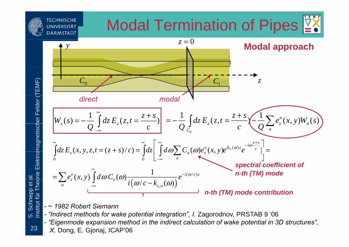
Modal Termination of Pipes0y 0z = Modal approach
TEM
F) z0C 1C
her F
elde
r (
1( ) ( , )z zz sW s dz E z t
∞ += − =∫1 1( , ) ( , ) ( )n
z z nz sdz E z t e x y W s+= − = − ∑∫
direct modal
mag
netis
ch
( ) ( , )z zQ c−∞∫
0
( , ) ( , ) ( )z z nnC
yQ c Q∑∫
( )( , , , ( ) / ) ( ) ( , ) n
z siik zn cdz E x y z t z s c dz d C e x y e eωωω ω
∞ ∞ ∞ +−⎡ ⎤= + = =⎢ ⎥∑∫ ∫ ∫
al.
orie
Ele
ktro
( )( / )1( , ) ( )n i c s
z ne x y d C e ωω ω∞
−=∑ ∫
0 0
( , , , ( ) / ) ( ) ( , )z n zn
dz E x y z t z s c dz d C e x y e eω ω−∞
+ ⎢ ⎥⎣ ⎦
∑∫ ∫ ∫spectral coefficient ofn-th (TM) mode
Schn
epp
et a
tut f
ür T
heo ( ),
( , ) ( )/ ( )z n
n z n
yi c kω ω−∞ −∑ ∫
n-th (TM) mode contribution
- ~ 1982 Robert Siemann
23
S. S
Inst
i 1982 Robert Siemann- “Indirect methods for wake potential integration”, I. Zagorodnov, PRSTAB 9 ‘06- “Eigenmode expansion method in the indirect calculation of wake potential in 3D structures”,
X. Dong, E. Gjonaj, ICAP’06
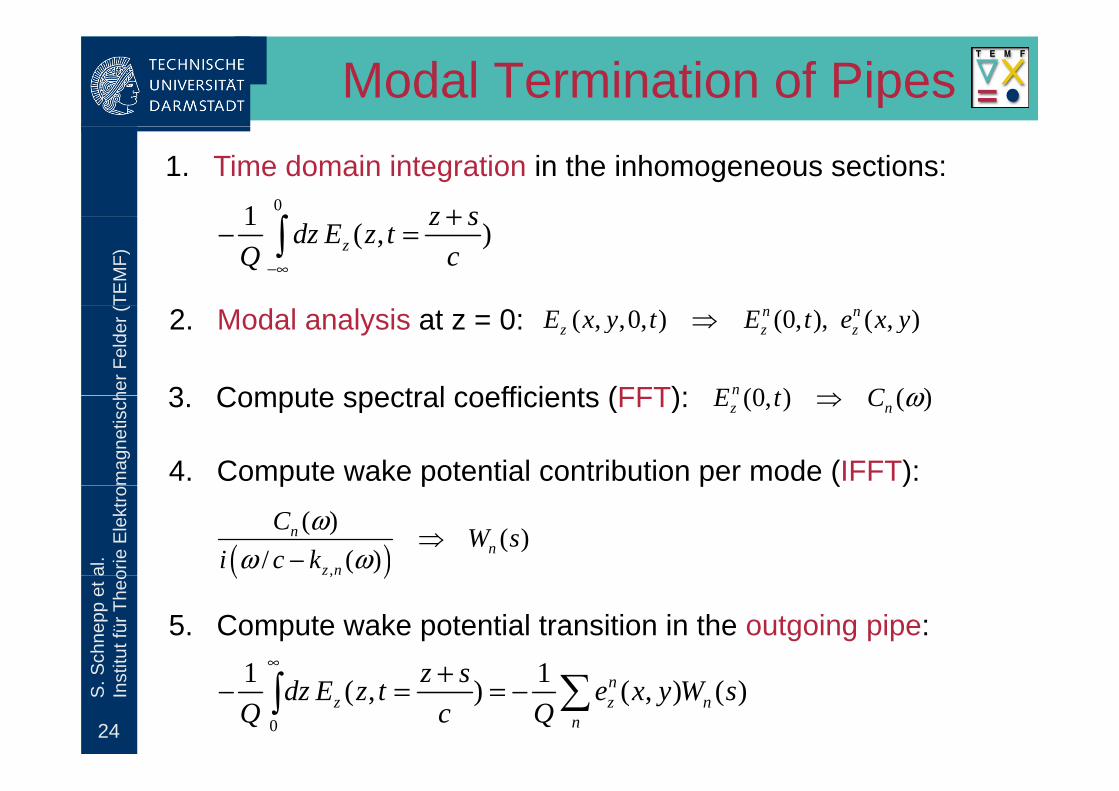
Modal Termination of Pipes1. Time domain integration in the inhomogeneous sections:
01 z s+∫
TEM
F)
1 ( , )zz sdz E z t
Q c−∞
+− =∫
her F
elde
r ( 2. Modal analysis at z = 0: ( , ,0, ) (0, ), ( , )n nz z zE x y t E t e x y⇒
3 Compute spectral coefficients (FFT): (0 ) ( )nE t C ω⇒
mag
netis
ch 3. Compute spectral coefficients (FFT): (0, ) ( )z nE t C ω⇒
4. Compute wake potential contribution per mode (IFFT):
al.
orie
Ele
ktro
p p p ( )
( ),
( ) ( )/ ( )
nn
z n
C W si c k
ωω ω
⇒−
Schn
epp
et a
tut f
ür T
heo ( ),
5. Compute wake potential transition in the outgoing pipe:1 1∞
24
S. S
Inst
i
0
1 1( , ) ( , ) ( )nz z n
n
z sdz E z t e x y W sQ c Q
∞ +− = = − ∑∫
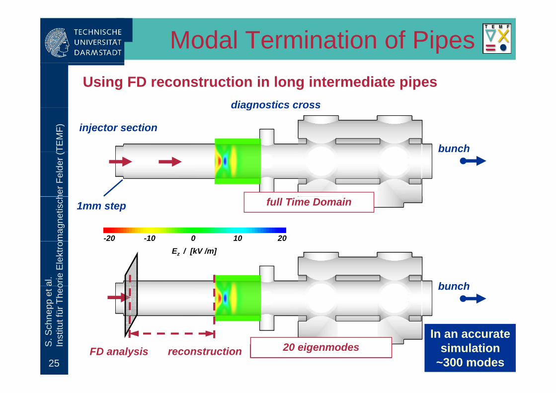
Modal Termination of PipesUsing FD reconstruction in long intermediate pipes
diagnostics cross
TEM
F)
bunch
injector section
diagnostics cross
her F
elde
r (
bunch
mag
netis
ch full Time Domain
-20 -10 0 10 20
1mm step
al.
orie
Ele
ktro
bunch
Ez / [kV /m]
Schn
epp
et a
tut f
ür T
heo bunch
I t
25
S. S
Inst
i
lowest eigenmode5 eigenmodes10 eigenmodes15 eigenmodes20 eigenmodesFD analysis reconstructionIn an accurate
simulation ~300 modes
Outline
•• IntroductionIntroduction
TEM
F)
•• IntroductionIntroduction
•• NumericalNumerical MethodMethod
her F
elde
r (
•• Parallelization StrategyParallelization Strategy
mag
netis
ch •• Modal Termination of Beam PipesModal Termination of Beam Pipes
•• PBCI SimulationPBCI Simulation ExamplesExamples
al.
orie
Ele
ktro
PBCI Simulation PBCI Simulation ExamplesExamples
Schn
epp
et a
tut f
ür T
heo
26
S. S
Inst
i
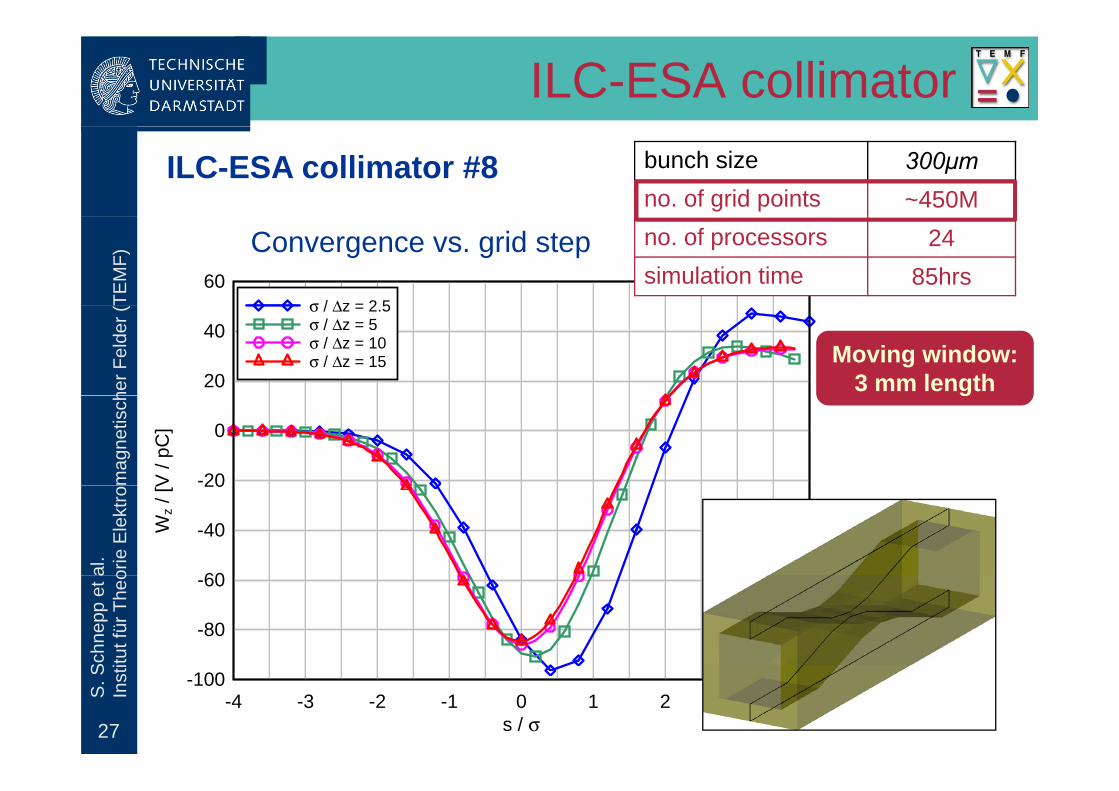
ILC-ESA collimatorILC-ESA collimator #8 bunch size 300μm
no. of grid points ~450M
TEM
F)
60σ / Δz = 2 5
Convergence vs. grid step no. of processors 24simulation time 85hrs
her F
elde
r (
20
40σ / Δz = 2.5σ / Δz = 5σ / Δz = 10σ / Δz = 15 Moving window:
3 mm length
mag
netis
ch
V /
pC]
-20
0
g
al.
orie
Ele
ktro
Wz /
[V
60
-40
20
Schn
epp
et a
tut f
ür T
heo
-80
-60
27
S. S
Inst
i
s / σ-4 -3 -2 -1 0 1 2 3 4
-100
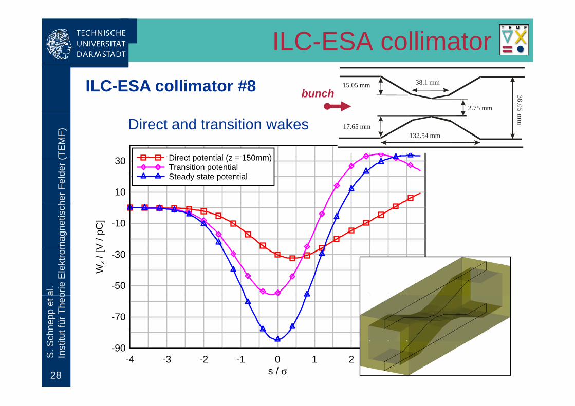
ILC-ESA collimatorILC-ESA collimator #8 38.05
38.1 mm15.05 mm
2.75 mm
bunch
TEM
F)
Direct potential (z = 150mm)
Direct and transition wakes
5m
m
132.54 mm17.65 mm
her F
elde
r (
10
30 Direct potential (z = 150mm)Transition potentialSteady state potential
mag
netis
ch
V /
pC] -10
al.
orie
Ele
ktro
Wz /
[V
-50
-30
Schn
epp
et a
tut f
ür T
heo
-70
28
S. S
Inst
i
s / σ-4 -3 -2 -1 0 1 2 3 4
-90
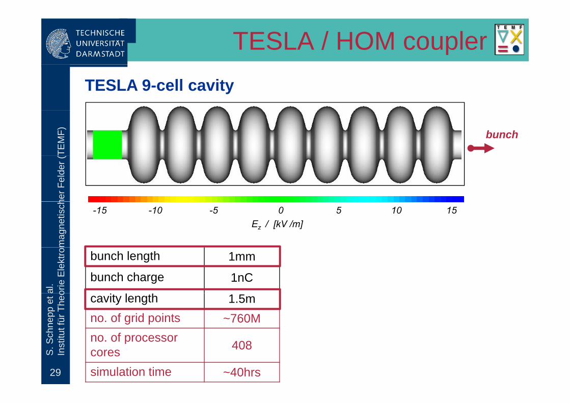
TESLA / HOM couplerTESLA 9-cell cavity
TEM
F) bunch
her F
elde
r (m
agne
tisch -15 -10 -5 0 5 10 15
Ez / [kV /m]
al.
orie
Ele
ktro bunch length 1mm
bunch charge 1nC
Schn
epp
et a
tut f
ür T
heo cavity length 1.5m
no. of grid points ~760Mno of processor
29
S. S
Inst
i no. of processorcores 408
simulation time ~40hrs
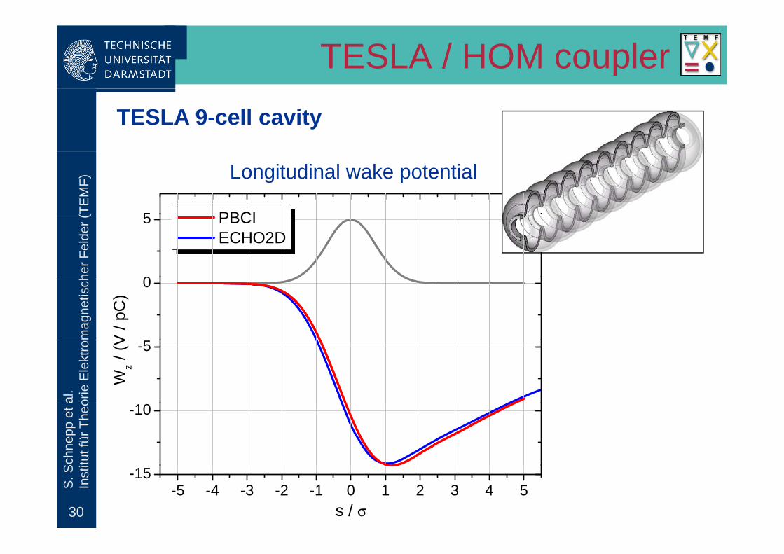
TESLA / HOM couplerTESLA 9-cell cavity
TEM
F) Longitudinal wake potential
5 PBCI
her F
elde
r (
0
5 PBCI ECHO2D
mag
netis
ch 0
V / p
C)
al.
orie
Ele
ktro -5
Wz /
(V
Schn
epp
et a
tut f
ür T
heo -10
30
S. S
Inst
i
-5 -4 -3 -2 -1 0 1 2 3 4 5-15
s / σ
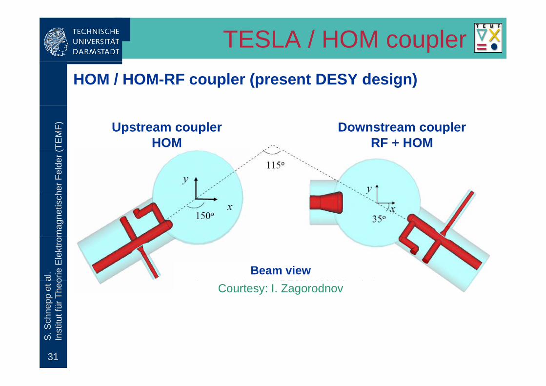
TESLA / HOM couplerHOM / HOM-RF coupler (present DESY design)
TEM
F) Upstream couplerHOM
Downstream couplerRF + HOM
her F
elde
r (m
agne
tisch
al.
orie
Ele
ktro
Beam view
Schn
epp
et a
tut f
ür T
heo
Courtesy: I. Zagorodnov
31
S. S
Inst
i
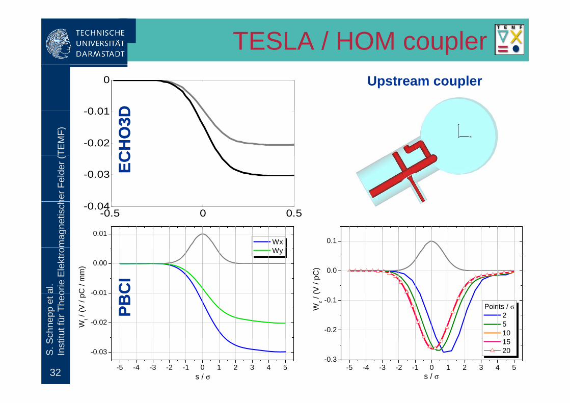
TESLA / HOM coupler
0 01
0
DD
Upstream couplerTE
MF)
-0.02
-0.01C
HO
3DC
HO
3D
her F
elde
r (
-0.03 ECEC
mag
netis
ch
-0.5 0 0.5-0.04
0.1
0.01
Wx
al.
orie
Ele
ktro
0.0
(V /
pC)
-0 01
0.00
C /
mm
)
Wy
CI
CI
Schn
epp
et a
tut f
ür T
heo
-0.2
-0.1
Wz /
(Points / σ
2 5 10
-0.02
-0.01
Wt /
(V /
pC
PBC
PBC
32
S. S
Inst
i
-5 -4 -3 -2 -1 0 1 2 3 4 5-0.3
s / σ
15 20
-5 -4 -3 -2 -1 0 1 2 3 4 5
-0.03
s / σ
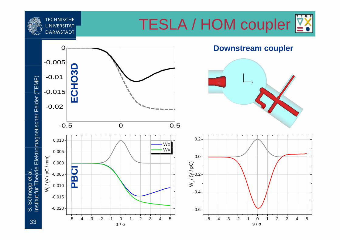
TESLA / HOM coupler
-0.005
0
DD
Downstream couplerTE
MF) -0.01
-0 015 CH
O3D
CH
O3D
her F
elde
r (
0.015
-0.02
ECEC
mag
netis
ch
0.010
Wx0.2
-0.5 0 0.5
al.
orie
Ele
ktro
-0 005
0.000
0.005
pC /
mm
)
Wy
-0 2
0.0
V /
pC)
CI
CI
Schn
epp
et a
tut f
ür T
heo
-0.015
-0.010
-0.005
Wt /
(V /
-0.4
-0.2 W
z / (V
PBC
PBC
33
S. S
Inst
i
-5 -4 -3 -2 -1 0 1 2 3 4 5
-0.020
s / σ
-5 -4 -3 -2 -1 0 1 2 3 4 5
-0.6
s / σ
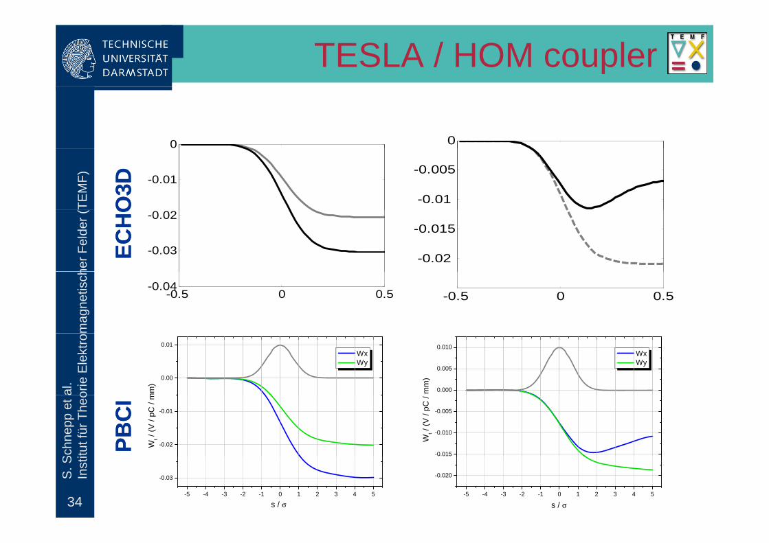
TESLA / HOM coupler
0 0
TEM
F) -0.01-0.005
-0.01 O3D
O3D
her F
elde
r (
-0.03
-0.02-0.015
-0.02 ECH
OEC
HO
mag
netis
ch
-0.5 0 0.5-0.04
-0.5 0 0.5
al.
orie
Ele
ktro
0.000
0.005
0.010
mm
)
Wx Wy
0.00
0.01
mm
)
Wx Wy
Schn
epp
et a
tut f
ür T
heo
-0.015
-0.010
-0.005
Wt /
(V /
pC /
-0.02
-0.01
Wt /
(V /
pC /
m
PBC
IPB
CI
34
S. S
Inst
i
-5 -4 -3 -2 -1 0 1 2 3 4 5
-0.020
s / σ -5 -4 -3 -2 -1 0 1 2 3 4 5
-0.03
s / σ
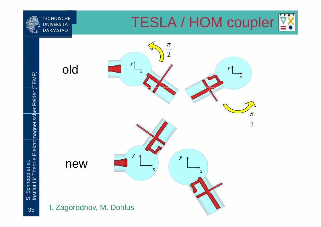
TESLA / HOM coupler
2π
TEM
F)
x
y
x
y
x
y
x
yold
her F
elde
r (
π
mag
netis
ch
2π
al.
orie
Ele
ktro
yyyy
new
Schn
epp
et a
tut f
ür T
heo
xxxxnew
35
S. S
Inst
i
I. Zagorodnov, M. Dohlus
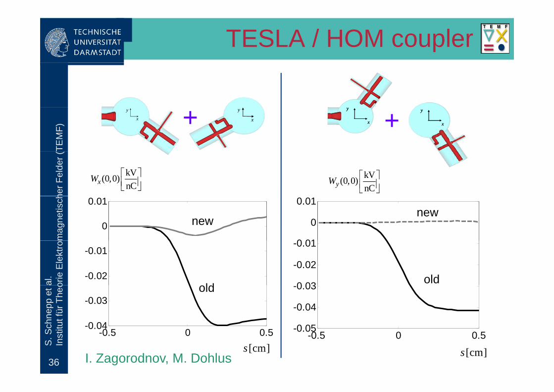
TESLA / HOM couplerTE
MF)
x
y
x
y
x
y
x
y+ x
y
x
y
x
y
x
y
+
her F
elde
r (
kV(0,0)nCxW ⎡ ⎤⎢ ⎥⎣ ⎦
kV(0,0)nCyW ⎡ ⎤⎢ ⎥⎣ ⎦
mag
netis
ch
0
0.01
0 01
0
0.01
newnew
al.
orie
Ele
ktro
-0.02
-0.01
0 03
-0.02
-0.01
ldold
Schn
epp
et a
tut f
ür T
heo
0 5 0 0 5-0.04
-0.03
-0 05
-0.04
-0.03old
36
S. S
Inst
i -0.5 0 0.5 -0.5 0 0.50.05
[cm]s [cm]sI. Zagorodnov, M. Dohlus
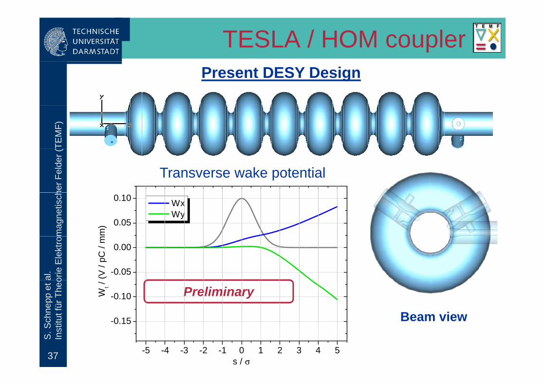
TESLA / HOM couplerPresent DESY Design
TEM
F)he
r Fel
der (
Transverse wake potential
mag
netis
ch
0.05
0.10 Wx Wy
m)
al.
orie
Ele
ktro
-0.05
0.00
(V /
pC /
m
Schn
epp
et a
tut f
ür T
heo
Beam view-0.15
-0.10Wt /
Preliminary
37
S. S
Inst
i
-5 -4 -3 -2 -1 0 1 2 3 4 5
0.15
s / σ
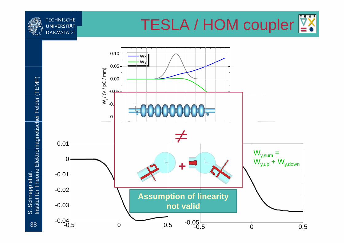
TESLA / HOM coupler
0 05
0.10 Wx Wy
TE
MF) +
-0.05
0.00
0.05
(V /
pC /
mm
)
her F
elde
r (
-0.15
-0.10Wt /
(
mag
netis
ch
0.01 0.01
-5 -4 -3 -2 -1 0 1 2 3 4 5s / σ≠
al.
orie
Ele
ktro
-0.01
0
-0.01
0Wx,sum =Wx,up + Wx,down
Wy,sum =Wy,up + Wy,down+
Schn
epp
et a
tut f
ür T
heo
0 03
-0.02-0.03
-0.02
Assumption of linearityt lid
38
S. S
Inst
i
-0.5 0 0.5-0.04
-0.03
-0.5 0 0.5-0.05
-0.04not valid
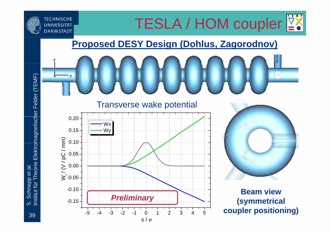
TESLA / HOM couplerProposed DESY Design (Dohlus, Zagorodnov)
TEM
F)he
r Fel
der (
Transverse wake potential0 20
mag
netis
ch
0 10
0.15
0.20 Wx Wy
m)
al.
orie
Ele
ktro
0.00
0.05
0.10
(V /
pC /
mm
Schn
epp
et a
tut f
ür T
heo
Beam view-0.10
-0.05Wt /
(
P li i
39
S. S
Inst
i
(symmetrical coupler positioning)-5 -4 -3 -2 -1 0 1 2 3 4 5
-0.15
s / σ
Preliminary
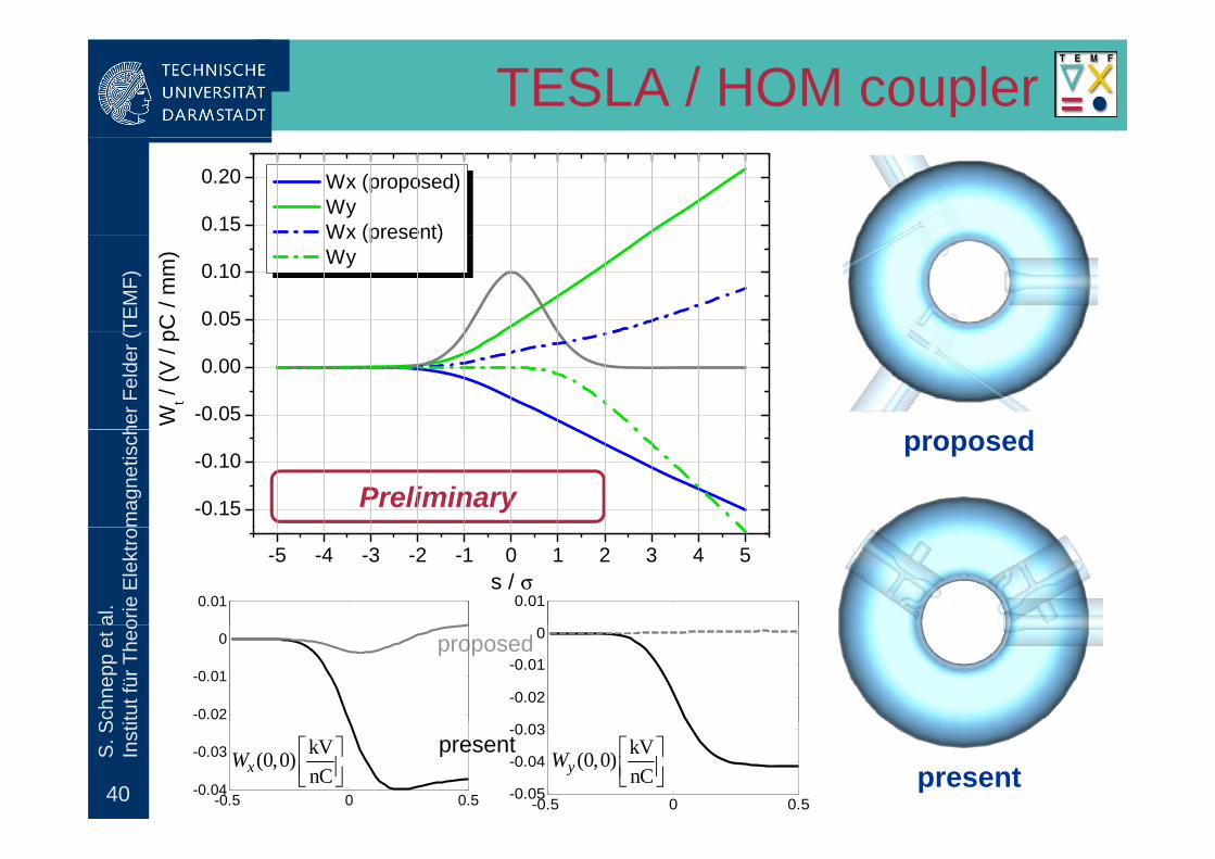
TESLA / HOM coupler
0.15
0.20 Wx (proposed) WyWx (present)
TEM
F)
0.05
0.10
Wx (present) Wy
pC /
mm
)
her F
elde
r (
-0.05
0.00
Wt /
(V /
p
mag
netis
ch proposed
-0.15
-0.10
Preliminary
al.
orie
Ele
ktro
0.01 0.01
-5 -4 -3 -2 -1 0 1 2 3 4 5s / σ
Schn
epp
et a
tut f
ür T
heo
-0.02
-0.01
0
-0.02
-0.01
0proposed
40
S. S
Inst
i
present-0.5 0 0.5
-0.04
-0.03
-0.5 0 0.5-0.05
-0.04
-0.03kV(0,0)nCxW ⎡ ⎤⎢ ⎥⎣ ⎦
kV(0,0)nCyW ⎡ ⎤⎢ ⎥⎣ ⎦
present
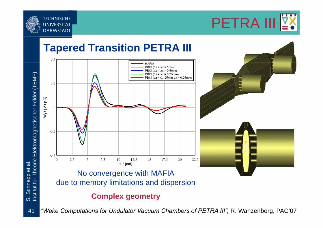
PETRA IIITapered Transition PETRA III
TEM
F)he
r Fel
der (
mag
netis
chal
.or
ie E
lekt
roSc
hnep
pet
atu
t für
The
o
No convergence with MAFIAdue to memory limitations and dispersion
41
S. S
Inst
i
Complex geometry
“Wake Computations for Undulator Vacuum Chambers of PETRA III”, R. Wanzenberg, PAC’07
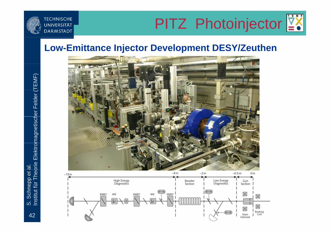
PITZ PhotoinjectorLow-Emittance Injector Development DESY/Zeuthen
TEM
F)he
r Fel
der (
mag
netis
chal
.or
ie E
lekt
roSc
hnep
pet
atu
t für
The
o
42
S. S
Inst
i
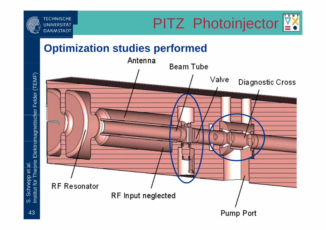
PITZ PhotoinjectorOptimization studies performed
TEM
F)he
r Fel
der (
mag
netis
chal
.or
ie E
lekt
roSc
hnep
pet
atu
t für
The
o
43
S. S
Inst
i
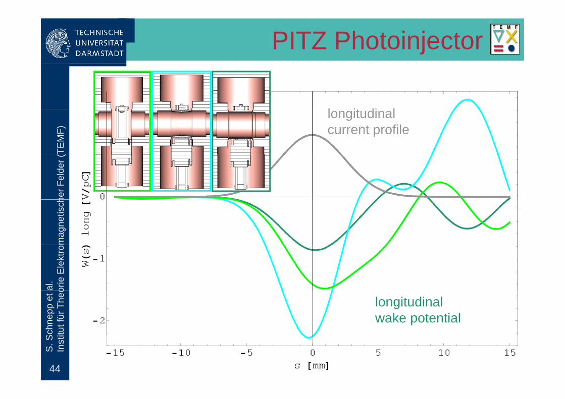
PITZ Photoinjector
l it di l
TEM
F)
longitudinalcurrent profile
her F
elde
r (m
agne
tisch
al.
orie
Ele
ktro
Schn
epp
et a
tut f
ür T
heo
longitudinalwake potential
44
S. S
Inst
i
PITZ PhotoinjectorTE
MF)
her F
elde
r (m
agne
tisch
al.
orie
Ele
ktro
Schn
epp
et a
tut f
ür T
heo
45
S. S
Inst
i
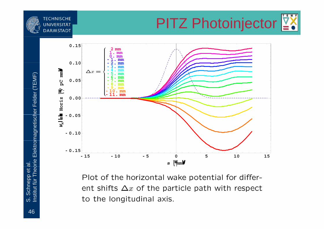
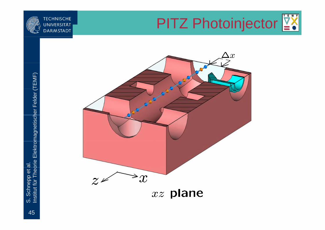
PITZ Photoinjector
0 10
0.152 mm1. mm0. mm
- 1. mm2 mm
TEM
F)
0.05
0.10V�pCmmD
- 2. mm- 3. mm- 4. mm- 5. mm- 6. mm- 7. mm- 8. mm- 9. mm
her F
elde
r (
0 05
0.00LHoriz@V 9. mm
- 10. mm- 11. mm
mag
netis
ch
- 0.10
- 0.05
WxHsL
al.
orie
Ele
ktro
- 15 - 10 - 5 0 5 10 15- 0.15
s @mmD
Schn
epp
et a
tut f
ür T
heo
46
S. S
Inst
i
PITZ Photoinjector
0.08
TEM
F)
0 04
0.06
her F
elde
r (
0.02
0.04
V�pCmmL
mag
netis
ch
- 0.02
0.00k xHV
al.
orie
Ele
ktro
- 10 - 8 - 6 - 4 - 2 0 2
- 0.04
Schn
epp
et a
tut f
ür T
heo - 10 - 8 - 6 - 4 - 2 0 2
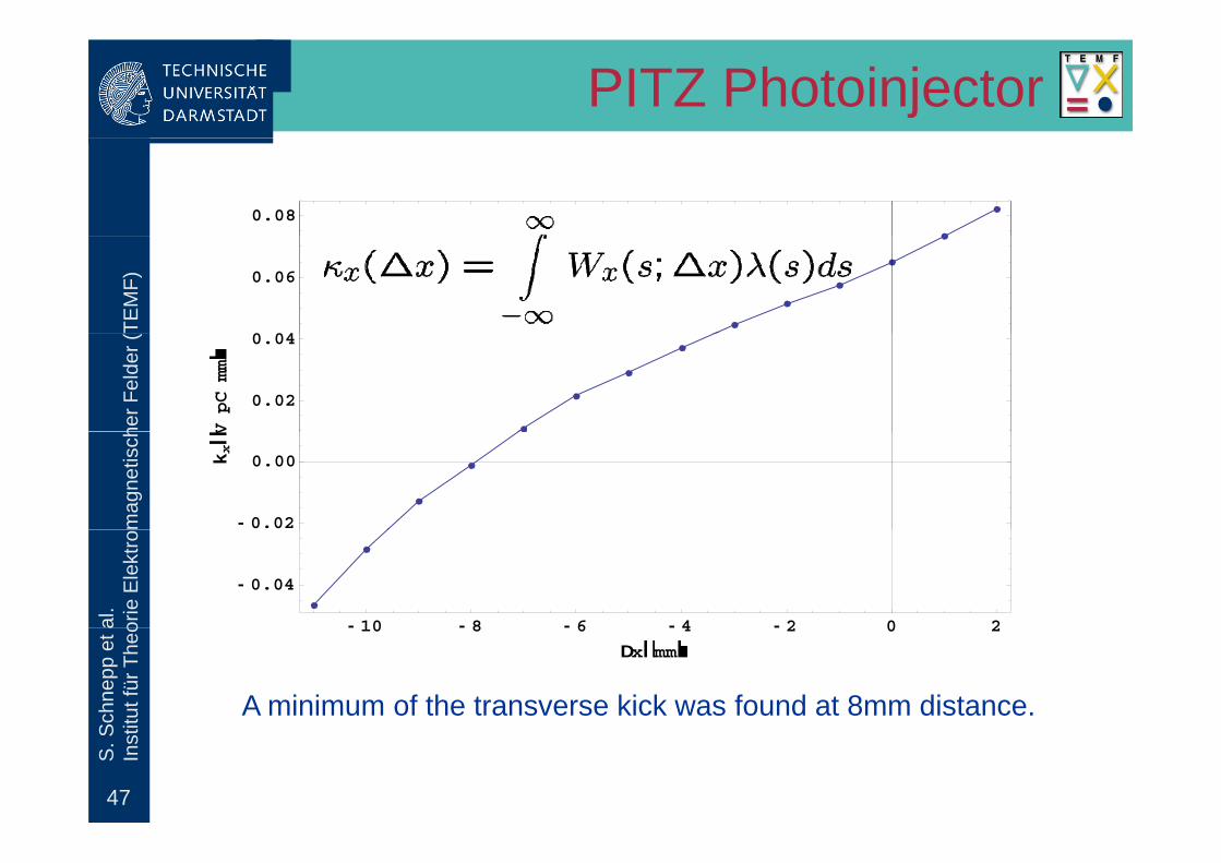
DxHmmLA minimum of the transverse kick was found at 8mm distance.
47
S. S
Inst
i
TEM
F) Large Scale 3D Wakefield Si l i i h PBCI
her F
elde
r ( Simulations with PBCI
mag
netis
ch S. Schnepp, W. Ackermann, E. Arevalo,E. Gjonaj, and T. Weiland
al.
orie
Ele
ktro
"Wake Fest 07 - ILC wakefield workshop at SLAC”11 13 D b 2007
Schn
epp
et a
tut f
ür T
heo 11-13 December 2007
Technische Universität Darmstadt, Fachbereich Elektrotechnik und InformationstechnikSchloßgartenstr. 8 , 64289 Darmstadt, Germany - URL: www.TEMF.de
Technische Universität Darmstadt, Fachbereich Elektrotechnik und InformationstechnikSchloßgartenstr. 8 , 64289 Darmstadt, Germany - URL: www.TEMF.de
S. S
Inst
i