Do Male-Female Wage Differentials Reflect Differences in the

Return to Skill? Cross-City Evidence From 1980-2000

Paul BeaudryUniversity of British Columbia and NBER

Ethan Lewis∗

Dartmouth College and NBER

April 2012

Abstract

Over the 1980s and 1990s the wage differentials between men and women (withsimilar observable characteristics) declined significantly. At the same time, the returnsto education increased. It has been suggested that these two trends may reflect acommon change in the relative price of a skill which is more abundant in both womenand more educated workers. In this paper we explore the relevance of this hypothesisby examining the cross-city co-movement in both male-female wage differentials andreturns to education over the 1980-2000 period. In parallel to the aggregate pattern,we find that male-female wage differentials at the city levels moved in opposite direc-tion to the changes in the return to education. We also find this relationship to beparticularly strong when we isolate data variation which most likely reflects the effectof technological change on relative prices. We take considerable care of controlling forpotential selection issues which could bias our interpretation. Overall, our cross-cityestimates suggest that most of the aggregate reduction in the male-female wage dif-ferential observed over the 1980-2000 period was likely due to a change in the relativeprice of skill that both females and educated workers have in greater abundance.

∗Comments welcome. The authors acknowledge the helpful comments of seminar participants at theUniversity of British Columbia, the Federal Reserve Bank of San Francisco, and Dartmouth College. MarkDoms was heavily involved in the early stages of this project, and we are indebted to him for his substantialinput. All errors are our own.

1 Introduction

Over the 1980-2000 period the US wage gap between men and women with similar char-

acteristics decreased significantly. Since 2000 this wage gap has stayed quite stable. There

are many proposed explanations for the observed decrease in the gender wage gap, includ-

ing increased positive selection of women into the labor market (Mulligan and Rubinstein,

2008), an improved match between actual and potential measures of experience (O’Neill and

Polacheck, 1993) – among other consequences of greater labor force attachment potentially

induced by increased access to birth control (Bailey, Hershblein, and Miller, 2012) – and

decreased discrimination.1 One especially intriguing observation is that the gender wage gap

has mirrored rather closely movements in the return to education over this period (see Figure

1), with the gender gap decreasing when the return to education increased.2 This has had

lead some researchers, most notably F. Welch (2000), to conjecture that the two patterns

may be driven by a common underlying force. According to this conjecture, men and women

(with similar education) bring to the market different bundles of skills, as do more educated

relative to less educated individuals. When methods of production change drastically – such

as with the introduction and diffusion of the PC – this changes the price of different skill

attributes which in turn induces movements in the gender wage gap and education wage

gaps, since both gaps compare the value of skill bundles. To be more precise, if individuals

are viewed as bringing to the market both soft-cognitive skills (or interpersonal skills) and

hard-motor skills (or brawn), and if women and more educated workers are both relatively

more endowed is such softer skills, then an increase in the relative price of soft versus hard

skills should cause the male-female wage gap to decrease at the same time as the return

to education increases. While some evidence lends support to this view, the literature on

gender gaps appears to remain skeptical of its relative importance in explaining the decrease

in the wage gap observed over the 1980s and 1990s, since the claim is backed-up foremost by

time-series evidence (which could easily be spurious) or else does not directly analyze gender

wage gaps.3 The object of this paper is to more thoroughly flesh out the empirical content of

1O’Neill and Polacheck (1993) also attribute some of the decline to a decrease in blue-collar wages. Genderdiscrimination is often mentioned, but, as it is difficult to quantify, its importance is not usually empiricallyassessed. For example, Blau and Kahn(2006) say that the larger unexplained portion of the decline in thewage gap in the 1980s compared to the 1990s may be evidence of a contribution of decreased discrimination,though they also consider other interpretations.

2The regression of the gender wage gaps in Figure 1 on the college-high school wage gap gives -0.625 forthe high school level gender gap and -0.787 for the college level gender gap.

3The evidence in support of this view includes the time series correlation between the male-female wagegap and the returns to education (such as in Figure 1; also Welch, 2000, and Fortin and Lemieux, 2000) the

2

this conjecture and then explore its implications for cross-city observations on gender gaps

and returns to education.

The idea that a change in the relative price of soft/cognitive skills versus hard/motor skills

could be behind some or all of the decrease in the gender wage gap observed over the 1980-

2000 period is a rather straightforward proposition. However, empirically evaluating its

relevance is hindered by the fact that the relevant relative price is not directly observable.

As we will show using a simple two attribute model, when female workers and more edu-

cated workers have relatively more soft-cognitive versus hard-motor skills than other types

of workers, then the relative price of soft versus hard skills plays the role of a common latent

factor that drives in opposite directions the gender gap and the return to education. The

main idea of this paper is to examine the quantitative relevance of this unobserved factor by

examining how city level measures of the gender gap and the return to education change in

response to forces that likely caused changes in the local price of these skills. If this common

factor is present, then the gender gap and the return to education should systematically co-

move in opposite directions in response to forces that affect the relative price of soft versus

hard skills.

The main challenge in implementing this simple idea is finding city level factors that plausibly

affects city level relative prices of skill.4 To make headway in identifying such factors, we refer

to the capital-skill complementarity literature which argues that 1980 to 2000 was a period

where the introduction of new capital equipment – most notably the PC – drastically changed

the relative price of certain skills since it acted as a substitute for many motor or hard skills,

and a complement for more cognitive skills.5 Based on this view, one may consider regressing

decline in wages in jobs which require motor skills and the rise in wages in jobs which require cognitive skills(Baccolod and Blum, 2010), and the correlation across industries between the change in female employmentshare and the adoption of computers, especially in blue collar jobs (Weinberg, 2000). Black and Spitz-Oener’s(2010) finding that a majority of women’s relative wage increases in Germany between 1979 and 1999 can beaccounted for by a large relative shift away from “routine cognitive” tasks (which Autor, Levy, and Murnane(2003) found was associated with computerization) is also consistent with the decline in the wage gap havinga technological origin.

4To identify the relevant co-movement, these factors must simultaneously be uncorrelated with otherresidual factors which may affect either the gender wage gap or the returns to skill.

5One view of recent technological change is that the PC is a “revolutionary” technology (Caselli, 1999) ofdiscretely higher skill intensity than previous technology; its adoption is therefore depends on comparativeadvantage: the relative price of (and therefore supply of) skill. This is empirically supported in Beaudryand Green, 2003, 2005; and Beaudry, Doms, and Lewis, 2010. Autor, Levy and Murnane (2003) alsomodel computer adoption as responding to skill ratios, and a version of their model will be the main modelof production we consider in this paper. Another view is that PCs are the latest example of ongoingimprovements in the quality of capital that favor skilled workers which perhaps goes back as much as acentury (Goldin and Katz, 2008).

3

city level observations of both changes in gender wage gaps and in returns to education on

measures of technological adoption — such as the local use of PCs – and see if these two

wage differentials move in opposite directions. While we will report the results of such an

exercise, such an approach is potentially problematic as technological adoption is itself an

endogenous process. For this reason, we also use insight from the endogenous technological

adoption literature (similar to that used in Beaudry, Doms & Lewis, 2010, hereafter BDL.)

to illustrate how local labor market conditions prior to the introduction of the PC can be

used as instruments for technology adoption. The main idea is that, if PCs complement soft

skills and substitute for hard skills, then they should be adopted most strongly in localities

where soft skills were initially relatively abundant. Hence this idea suggests that the city

level change in the gender wage gap and the return to education should respond in opposite

directions to measures of a city’s pre-PC-era relative abundance of these skills.

Using data from the 1980 and 2000 Censuses of Population, we begin by examining whether

the gender wage gap and the return to education moved in opposite directions across cities

during this period. Interestingly, we find that the cross-city evidence echoes the time series

pattern of strong negative co-movement, thereby providing initial evidence supporting the

conjecture that the gender wage gap and the return to education may be driven by a common

latent force. However, based on OLS estimates, the cross-city co-movement is substantially

weaker than that found in the time series. We then exploit the insights of the endogenous

technological adoption literature in the presence of capital skill complementarity to explore

instrumental variable estimates of this relationship. Again, this class of models suggest that

cities where soft skills were most abundant “pre-PC” (in 1980) should be the same cities

where PCs are adopted most rapidly, inducing a greater increase in the return to education

and a greater decrease in the gender gap. We report evidence in support of each element

of this process. Our main finding is that, once we isolate variation in the wage data more

likely driven by changes in the relative prices of unobserved skills, we find that the cross-city

link between gender wage gap and the return to education to be very similar to that found

in the time series. We then use the cross-city evidence to help answer our initial time series

question. Our results suggest that most of the aggregate reduction in the male female wage

differential observed during the 1980-2000 period can be attributed to the change in a latent

relative price of a skill which is more abundant in both female and more educated workers.

The remaining sections of the paper are structured as follows. In Section 2 we present the

simple theoretical structure which guides our approach to the data. The theory encompasses

4

two elements: first, we clarify how gender gaps and returns to education are related in a

two attribute model of wage through a common latent factor. Then we use insights from

the literature on capital-skill complementarity and endogenous technological adoption to

discuss the identification of the effects of the common latent factor. Section 3 presents the

data used to examine determinants of the gender wage gaps and discusses implementation

and identification issues. Section 4 presents our main results and Section 5 discusses their

implication for aggregate changes. In the empirical analysis we examine in depth issues

of selection that may bias our results as such issues are thought to be potentially very

important in the behavior of the gender wage gap over our period of interest (see Mulligan

and Rubinstein, 2008). Finally Section 6 offers concluding comments.

2 Theory

The idea we want to evaluate is whether changes in the gender wage gap and in the return

to education may be driven by a common underlying force reflecting the price of a skill

which is relatively more abundant among women and more educated workers. In particular,

the main hypothesis is that the role of this common factor driving the gender wage gap

became most evident during the 1980-2000 period when technological change – as reflected

in the diffusion of PCs– considerably changed relative prices of skills. The object of this

section is to present a simple theoretical structure which will clarify how we can use cross-

city variation in wage outcomes to examine the issue. As noted in the introduction, there

are two distinct components which underly the theory. On the one hand, there is the notion

that wages reflect payments to bundles of skills. On the other hand, there is the idea that

the diffusion of PCs tended to increase the relative price of cognitive-soft skills because of its

complementarity to such factors, while it acts as a substitute for more routine-hard skills.

We now present each of these elements in turn in order to derive estimating equations and

associated instrumental variable strategies.

2.1 The gender wage gap and the returns to education in a twoattribute model

To begin, consider an environment where each worker brings to the market a two dimensional

vector of skills. The two components will be referred to as cognitive-soft skill (denoted S)

5

and raw labor (denoted L). Individuals differ in the amount of each skill they possess.

Let γSeg represent the amount of cognitive skill embodied in a a worker with education e ∈{e1, e2, ..., eN} and gender g ∈ {m, f}, and let γLeg represent the amount of raw labor embodied

in the same individual. For an individual in city c at time t his wage will be given by

Wegct = (γSegwSct + γLegw

Lct)ηegct,(1)

where wSct and wLct are the local prices of the cognitive skill and of raw labor respectively at

time t, and ηegct combines any systematic discrimination θegt (that can potentially vary over

time by gender and education) and a pure measurement error term νegct ( ηegct = θegt+νegct).

For now, we need not focus on why people with different skills may cluster more in some

locations than others. Instead, we can take the cross-city distribution of worker types as

given and postpone a discussion of the related endogeneity issues.

The main difficulty with using equation (1) is that none of the right hand side terms are

directly observable. Nonetheless, we can pursue some of its empirical implications by exam-

ining wage gaps across individuals. We begin with the male-female log wage gap at education

level e, which we denote MFdiffect. From (1), this can be expressed as

MFdiffect = lnWemct − lnWefct

= lnγLemγLef

+ ln

(1 +

γSemγLem

wSctwLct

)− ln

(1 +

γSefγLef

wSctwLct

)+ ln ηemct − ln ηefct

≈ lnγLemγLef

+

(γSemγLem−γSefγLef

)wSctwLct

+ ln ηemct − ln ηefct,

or, to simplify the notation, we can express it as:

MFdiffect ≈ α1e + β1

ePSct + εect,(2)

where α1e = ln γLem

γLef

, β1e = γSem

γLem− γSef

γLef

, P Sct =

wSct

wLct

, and εect = ln ηemct − ln ηefct. Equation

(2) says that the cross-city differences in the male-female wage gap depend on a common

education group effect and varies across cities because of differences in the relative price of

6

skills, P Sct . Similarly, the within gender wage gap between education levels ej and ei can also

be expressed as a function of the relative price of skills.

Ejidiffgct = lnWejgct − lnWeigct(3)

≈ α2jig + β2

jigPSct + εejigct

with α2jig = ln

γLejg

γLeigand β2

jig =γSejg

γLejg− γSeig

γLeigand εeijgct = ln ηeigct − ln ηejgct.

Equations (2) and (3) illustrate that in a two attribute model, both the gender wage gap

and the returns to education are linked by the relative price of skills which acts as a latent

common factor. Moreover, if we are willing to assume that at a given level of education men

have a smaller ratio of soft skills to raw labor (which implies β1e < 0) and that within gender

more educated workers have have relatively more soft skills (so if ej > ei, then β2jig > 0),

then we see that change in the relative price of skills P S will cause the gender wage gap and

the returns to education to move in opposite directions.

Although (3) and (2) still cannot be directly estimated, part of what we will exploit in esti-

mation is changes in the prices of skills during the era of PC diffusion. So taking differences

of (3) and (2) we get:

∆MFdiffec ≈ β1e∆P

Sc + ∆εec(4)

∆Ejidiffgc ≈ β2jig∆P

Sc + ∆εejigc(5)

Note that the error terms in (5) and (4) may not have a zero mean as they potentially

contain changes in systematic discrimination (changes in θegt). If we substitue (5) into (4) to

eliminate the unobserved skill price, we get the following relation between the gender wage

gap and the returns to education:

∆MFdiffgec ≈β1e

β2jig

∆EjiDiffgc + ∆εec −β1e

β2jig

∆εejigc(6)

7

Our conjectures about skill endowments imply β1e/β

2jig < 0. 6 One of our main goals will be

to estimate (6) consistently, as this will be necessary to help evaluate the role of changes in

skill price for explaining aggregate changes in the gender wage gap. However, even leaving

aside the potential endogeneity of cross-city wage variation in (6), the fact that wage gaps are

likely measured with error implies OLS estimates of β1e/β

2jig will be substantially attenuated.

In order to estimate (6) consistently, we will therefore need instruments for the returns to

education that reflect changes in the relative price of skill ∆P S. For this reason, we now

discuss how we can use insights from the capital-skill complementarity literature to find such

instruments.

2.2 Production and Endogenous PC Adoption

In order to discuss factors determining the relative price of skills, consider an environment

where there is only one produced good and where prices reflect marginal products. Initially,

the good is produced using only the skills of different workers. Then we consider the in-

troduction of a new capital good which is meant to capture the introduction of PC’s. Our

aim is to highlight how this affects the price of the two different skill attributes. For exposi-

tional simplicity, we follow Autor, Levy , and Murnane (2003) (hereafter, ALM) and model

the economy after the arrival of computing technology with the following Cobb-Douglass

production structure:

Qc = A(µPCc PCc + Lc

)αS1−αc(7)

where Qc represents aggregate output, Lc is the aggregate level of raw labor supplied by the

different individuals hired in market c, Sc represents the aggregate amount of soft skilled

hired in market c, PCc represents the use of personal computers, and α ∈ (0, 1). The only

way in which this production function differs from ALM is the factor loading µPCc , which

we include to capture potential city-specific productivity differences in the use of PCs.7 The

important element of this technology is that PCs substitute for raw labor and complement

the soft-cognitive skill. The results we exploit in what follows relies on this assumption but

not on the particularly restrictive functional form given by 7.8

6β1e/β

2jig < 0 may vary across education groups, which we will allow for in some of our estimates, but we

will restrict it to be constant in our main discussion.7In ALM, this production function represented many industries, each with different αs.8See Beaudry, Doms and Lewis (2010) for a more general discussion.

8

Now, consider a period before the arrival of PCs, which we will call t = 1980 to match our

empirics below. We model this by setting µPCc = 0, so Qc = ALαcH1−αc . This implies that

before the arrival of PCs, the relative price of soft skills versus raw labor is given by:

P Sc,1980 = ln

wSc,1980wLc,1980

= lnα

1− α− ln

(Sc,1980Lc,1980

)= ln

α

1− α− lnsc,1980(8)

where sc,1980 = Sc,1980

Lc,1980. Equation (8) simply indicates that the relative price of soft skills

prior to the introduction of PCs was negatively related to the local abundance of soft skills.9

After the arrival of the PC, which we assume is available in all localities at the same price

(denoted P PC), we can express the change in the relative price of skills in two different

manners depending on whether or not we use the optimally condition for the determination

of PCs which is given by:

ln(αµPCc A

)− (1− α) ln

(µPCc

PCcLc

+ 1)

+ (1− α) ln sc = lnP PC

If we use this optimally condition in conjunction with the marginal product conditions for

each skill, we can express the change the in the price of skill as:

∆ lnP Sc =

ln (αA)− lnP PC

1− α+ ln sc,1980 +

ln(µPCc

)1− α

(9)

Equation (9) indicates that the change in the relative price of skill at the city level will be

greatest where its relative supply is initially most abundant (i.e. where sc,1980 is greatest).

This property reflects the capital-skill complementary of the arrival of the PC.10 Before the

arrive of the PC, regions with more soft-cognitive skills have a relatively low price for this

skill and a high price for hard skills. This makes the adoption of PCs very attractive in such

a market. Therefore, PCs should be adopted more aggressively in such market causing the

relative price of soft skill to increase most where soft skills are initially more abundant. If

we use (9) to replace ∆P S in 4 and 5 we get

∆MFdiffec = β1e

ln (αA)− lnP PC

1− α+ β1

e ln sc,1980 + β1e

ln(µPCc

)1− α

+ ∆εec(10)

9This property holds for a wide variety of production setups and we can easily generalize the structureas not to obtain a unit elasticity.

10This property does not rely on the particular functional form of the production function but does dependson the arrival a new technology where the PC is a complement to soft skills and a substitute to hard skills.

9

∆Ejidiffgc = β2jig

ln (αA)− lnP PC

1− α+ β2

jig ln sc,1980 + β2jig

ln(µPCc

)1− α

+ ∆εejigc(11)

The interesting aspect of these two equations is that they now contrast how cross-city move-

ments in the gender wage gap and the returns to education will respond differently to a

potentially observable aggregate factor: the relative supply of skills. In particular, these

equations indicate that following the introduction of the PCs, we should see the gender wage

gap fall most in cities where soft skill were most abundant prior to the arrival to the PC

(since, again, β1e < 0). Moreover, it indicates that we should simultaneously see the greatest

increase in the return to education precisely in these same cities. If we have a measure of

these relative skills, then in principle we can estimate (10) and (11) consistently by OLS un-

der the assumption that the local skill supply prior to the arrival of PC was not anticipating

which cities would be best at using PCs (ie, the skill supply in 1980 is not systematically

related to µPCc ). These two equations also suggest that one way of estimating equation (6)

is to use measured skills in 1980 as an instrument for ∆EDijdiffc. This should also allow

for consistent estimates under the assumption that skill supply in 1980 did not forecast PC

efficiency across cities.

While equation (9) offers a simple and useful way of linking changes in the relative price of

skill and initial skill supplies, it hides much of the mechanism underlying the the model. In

particular, by using the optimality condition for the adoption of PCs, we have somewhat

obscured the fact that it is the adoption of the new technology that– according to the capital-

skill complementarity view– is causing the opposite movements in the gender wage gap and

the returns to education. In order to see these intermediate forces more explicitly, it is useful

to express the change the relative price of skill using only marginal product conditions for

each skill. In this case, we can express the change in the relative price of skill as

∆P Sc ≈

PCcLc−∆ ln sc + µPCc(12)

Now using 12 to replace the price of skill in 4 and 5, we obtain

∆MFdiffec ≈ β1e

PCcLc− β1

e∆ ln sc + β1eµ

PCc + ∆εec(13)

∆Ejidiffgc ≈ β2jig

PCcLc− β2

jig∆sc + β2jigµ

PCc + ∆εejic(14)

10

Equations (13) and (14) now makes more explicit the relationship between the gender wage

gap, returns to education and technological change. In particular, these equations indicate

that greater PC adoption should be associated with a greater reduction in the gender wage

gap and a greater increase in the return to education. Moreover, it suggests that a faster

increase in the relative supply of skills should be associated with increases in the gender

wage gap and decreases in the returns to skill. The difficulty with these two equations,

relative to equations (10) and (11), is that they are much more prone to endogenity. In

particular, observed adoption of PCs will be correlated with local efficiency of PC use (µPCc ).11

To address the endogeneity of PC adoption, we use 1980 measures of skill supply as the

instruments, under the assumption that pre-PC-era skill supplies were not anticipating PC

efficiency. The formulation given by equations (13) and (14) also highlight the potential

use of PC adoption as an instrument for estimating equation (6). Although PC adoption is

endogenous and correlated with µPCc , this terms does not enter the error term in equation

(6) and hence is potentially a valid candidate as an instrument.

In summary, our model of capital-skill complementarity in a two attribute model has high-

lighted different factors that should cause opposite movements in the gender gap and the

returns to education. Furthermore, the model has provide insight regarding what instru-

ments are potentially admissible for exploring these relationships. In the empirical section

we will examine these implications to show that the ideas behind this simple model find

considerable support in the data. Once this is shown, we will discuss how the estimated

relationships based on cross-sectional observation can be used to evaluate the role of skill

price changes in explaining the decrease in the aggregate gender wage gap observed over the

1980-2000 period.

3 Data and Empirical Methods

Our empirical investigation will focus on estimating the main relationships described in the

previous section (these are equations (6), (10),(11), (13) and (14)) using data on aggregate

outcomes drawn from U.S. metropolitan areas. We will begin this section by discussing the

data and then we will further discuss implementation and identification issues.

11The change in the local supply of skill is also possibly correlated with the error terms in (13) and (14),something we will discuss further below.

11

3.1 Data and Measures

Our goal is to estimate three types of relationships across 230 U.S. metropolitan areas. First,

the relationship between male-female and education wage gaps as described in (6). Second,

the relationships between the pre-PC era supply of skill and each of the two wage gaps –

the gender gap and the returns to education – as described in (10) and (11). And finally the

relationship between the use of PCs and the two wage gaps as described in (12) and (13).

To this end, we compute wages and skill supplies “pre-PC” using the 5% public-use version

of the 1980 Census of Population (Ruggles et al., 2010), and “post-PC” using the 2000

Census of Population. Skill mix was constructed using only data on those aged 16-65 with

positive (potential) work experience (age - years of schooling - 6 > 0), not living in group

quarters. Hourly wages were constructed for the further subsample with positive wage and

salary earnings and hours worked in the past year, without any self-employment earnings,

currently employed and not in school. Hourly wages were “Windsorized” to be between two

and 200 dollars in 1999 dollars.

Male-female wage gaps are constructed separately for five education groups that can be

consistently identified across censuses: high school dropouts, high school graduates, those

with some college education (but less than four years), four-year college graduates, and

advanced degrees.12 Wages are regression adjusted, separately by gender, education group,

and year, for a quartic in potential work experience and dummies for foreign-born, black,

Hispanic, and being born after 1950 (where Lemieux, 2006, describes a cohort break in trends

in returns to schooling.) To account for heterogeneity in years of education among workers

in the dropout, some college, and advanced degree groups, we also includes a linear control

for years of education and its interaction with the dummy for being born after 1950 for these

groups.13 To make the means interpretable, adjusted wages are centered on the predicted

values for the average female characteristics (in our whole sample of metropolitan areas) in

each year.14

12In the 1980 Census, “high school” and “college” workers are defined as those who have completed exactly12 years and 16 years of schooling, respectively, and in the 2000 Census, are those who report being in thecategory “high school graduate” and “Bachelor’s degree.”

13In neither census is there literally a “years of education” variable, but categories of years (1980) or degrees(2000). Within these three education groups with heterogeneous education, the grouping of education is quitedifferent in the two censuses. In both cases, we impute years from the midpoint of the categories in thegroup.

14In equation form, we estimate lnWiegct = aegct + β′egtXiegct + uiegct, where lnWiegct is the natural loghourly wage of person i of education group e and gender g living in city c in year t, which is regressed onfixed effects, aegct, and the adjustment variables, Xiegct, mentioned above. This is evaluated at the national

12

The main education wage gap we use on the right hand side is the simple average of male

and female adjusted college-high school wage gaps (which come from the same adjustment

procedure). We use the average to avoid any possibility of there being a “mechanical”

relationship between the left- and right-hand side wage gaps.

Our empirical implementation of the quantities of “soft-cognitive skill ” and “raw labor”

consists of the following. First, raw labor input is assumed to vary only with gender and not

with education, and we normalize γlf = 1, so γlm can be written as 1 + Θ , for some Θ > 0,

which will be estimated from average male-female wage gaps (described below). Letting `Mct

and `Fct represent aggregate hours worked by men and women, respectively, in local labor

market c in year t, we therefore define

Lct = (1 + Θ)`Mct + `Fct.(15)

Next, we impose that cognitive skill is linearly increasing in years of education above ten

years (and is flat below that) by the same amount for both genders, which roughly describes

the relationship between wages and education by gender (see Figure 2). That is, we define

Sct =∑e

λ ·max[(e− 10, 0)]`ect,(16)

where `ect represents the aggregate hours worked of all persons with e years of schooling

living in metropolitan area c and year t, and λ is the return to schooling.

To obtain estimates of Θ and λ we use the wage sample with more than 10 years of education

in the 1980 Census to estimate an individual level regression of ln(hourly wage) on years of

schooling and a male dummy. The coefficient on schooling is λ = 0.077, and on the male

dummy is Θ = 0.423. Substituting these into (15) and (16) generates our estimates of Lct

and Sct and our skill mix measure, sct = Sct/Lct. Note that this translates education and

hours worked into human capital using fixed coefficient in all cities and years. (The choice

of λ, in particular, is immaterial.)

This skill mix measure may appear unusual, and it imposes the extreme assumption that

gender wage gaps are entirely driven by gender differences in raw labor input per hour.15

female mean Xeft, and thus the adjusted male-female wage gap in education group e, city c and year t is

given by yect = aemct − aefct + (βemt − βeft)′Xeft.15For example, controlling for a gender-specific quartic in potential experience reduces the estimate of Θ

to 0.12.

13

However, Figure 3 shows that, in both 1980 and 2000, it is highly correlated with a more con-

ventional skill mix measure used in studies of the effect of computerization on skill demand:

the natural log of the ratio of college “equivalent” to high school equivalent hours.16 In that

figure, each circle represents one of the 230 metropolitan areas in our final sample. Circle

sizes are proportional to the 1980 population, the weights used throughout the analysis. Our

analysis will also construct standard errors to be asymptotically robust to arbitrary error

correlation within metropolitan area (across skill groups) and to heteroskedasticity.

Our measure of computerization is personal computers per worker at the average employer

in the metropolitan area, adjusted for three-digit (SIC) industry crossed with size category

dummies. The underlying data are firm level data collected by the marketing firm Harte-

Hanks in 2000 and 2002. For simplicity, we will refer to this as “2000” data.

(Weighted) summary statistics on our metropolitan-level wage gap and skill mix measures

are shown in Table 1. In each year there are 1,150 observations on the male-female wage gap

from 230 metropolitan areas and five education groups. As has been documented elsewhere,

the male-female wage gap declined over this period, by about 12 log points in our data.

This decline was largest between less-educated men and women. Table 1 also shows there is

“something to be explained” - there is variation in the level and change in the gender wage

gap across labor markets, even within education group, which itself is perhaps a new fact.

We now ask whether it is related to skill mix in the way the model suggests.

3.2 Further Identification issues

There are at least three additional issues we want to discuss as they could bias our inferences.

First, there is Mulligan and Rubinstein’s (2008) (MR) claim that rising returns to skill in-

duced differential entry of high skill women into the labor market, shrinking the gender wage

gap through change in the selection of working women from negative to positive. Second,

there is Mincer and Polacheck’s (1974) view that the gender wage gap results from women

interrupting their careers to have children, or put in labor economists’ terms, because they

had low actual work experience for a given amount of potential work experience compared

16As in Card(2009), Figure 3 defines college equivalents as those with a four year degree plus 0.4 shareof those with 1-3 years college. High school equivalents are 0.6 share of those with 1-3 years college, plusall of those with exactly 12 years, plus 0.7 share of those without a high school degree. (The fractionaldivisions derive from the workers in an education group supplying less than one efficiency unit per hourand/or dividing their labor supply between college and high school tasks.)

14

to men. This gap in actual work experience may have diminished over time as women had

more continuity in their careers, shrinking the wage gap.17 Third, there is the possibility

that a decline in discrimination just happened to occur at the same time as the diffusion of

PCs.

In our view, the most important source of potential bias comes from the MR story. In our

model, education and male female wage gaps are negatively correlated because of common

unobserved skill prices, but in the MR story they are related for a different reason: high

returns to skill differentially induce high skill women to enter the workforce. In this view,

the arrival of computers could still reduce the male-female wage gap, but through changes in

selection (rather than through changes in the “quality constant” male-female wage gap).18

We do three things to address this type of selection. First, we will include estimates that

control for selection in a manner similar to the way MR did. We will use an inverse mills

ratio transformation of the predicted probability of female employment, using the presence

of kids under age six in the household (whose effect is allowed to vary by marital status)

as an instrument for female employment. Further details on this estimation strategy are

below. In keeping with MR, this selection correction is allowed to vary by year, and in our

case, regionally. Second, also like MR, we will examine groups of women whose employment

is likely less sensitive to the wage structure, including single women without kids. Third,

and more simply, we control for female employment rates. As these could be endogenous

outcomes of wages, however, we use and interpret these controls cautiously.

As for other potential sources of decline in the male-female wage gap, while we are not a

priori ruling out that systematic differences in work experience or gender discrimination bias

our estimates, there is no clear reason why these should be correlated with our right-hand

side variables. Nevertheless, we want to address these potential biases to the extent possible.

To minimize the influence of unobserved differences in actual (rather than potential) female

work experience across markets and over time, i.e., to address the Mincer-Polachek type

story, all of our wage gaps are adjusted for for gender (x education x year)-specific potential

17In addition, the diffusion of new birth control technology may have driven some of these other purportedchanges (Goldin and Katz, 2002; Bailey, 2006). In particular, Bailey, Hershblein, and Miller (2012) provideevidence that early legal access to the birth control pill induced women to increase the total hours workedby a given age, among other investments in skills.

18MR do not take a stand on what is generating the changes in the return to skill. Note that even in theMR story, selection may or may not bias our estimates: our male-female wage gaps condition on education(in addition to other observables, described below), so the MR-type bias will arise only if residual wage gapsare also larger in more high skilled cities. In addition, we are attempting to identify factor-supply, ratherthan demand, driven differences in education wage gaps.

15

experience profiles. To help control for changes in gender discrimination, we will include

estimates that control for state fixed effects, which capture the effect of any state-level

legislation improving the rights of women.

A fourth, more general, critique of our estimation approach is that there may be systematic

demographic or compositional differences correlated with skill mix and changes in the relative

wages of females. One plausible source of potential bias is differences in industry mix across

metro areas. Olivetti and Petrongolo (2011) find that differences in industry mix can account

for a substantial portion of cross-country differences in the gender gap. In addition, during

this time period the decline in the wages of less-skilled men in manufacturing could have

simultaneously lowered male-female wage gaps and raised college-high school wage gaps in

manufacturing-intensive locales (which is correlated with being a less-skilled locale).19 While

some of this might be due to technological change, some of it might be due to other forces

(like a decline in union power). Therefore we will control for measures of industry mix, and

manufacturing share in particular (described below). To address the possibility that other

types of compositional differences drive the results, we will also evaluate the sensitivity of

our estimates to controls for demographic mix (e.g., black share, immigrant share) and other

city characteristics.

4 Results

4.1 Ordinary Least Squares

Columns (1)-(7) of Table 2 shows OLS estimates of the relationship in equation (6), between

changes in the male-female and college-high school wage gaps between 1980 and 2000, with

various sets of controls. The controls have been demeaned so that the intercept, which

is shown, can be interpreted as the counterfactual change in the male-female wage gap

in a location with the average value of controls but no increase in the returns to college.

(See Section 5, below.) The estimates also pool together gender wage gaps for our five

different education categories (and, again, standard errors are calculated to be robust to

error correlation across education groups in a metro area).

Controlling only for education group effects (which by definition make no difference to the

19O’Neill and Polachek (1993) find that the decline in blue collar wages accounts for a quarter of thedecline in the male-female wage gap in the 1980s.

16

point estimates, since the education wage gap does not vary across education groups) pro-

duces a coefficient of -0.231, or that a one percentage point increase in the return to college is

associated with a 0.231 percentage point decline in the male-female wage gap. Despite having

(what is likely a very) noisy right-hand side variable, this relationship is highly significant.

Other columns of Table 2 add controls. In light of Olivetti and Petrongolo (2011), we believe

that it may be important to control for industry mix. So in columns (2)-(4) we explore three

different versions of industry mix controls. To begin with, we control for durable and non-

durable manufacturing employment shares, measured in 1980, whose impact is allowed to

vary by the two, what we will call “broad,” education categories that Olivetti and Petrongolo

(2011) used: (1) workers with some college or below or (2) four years of college or more.20 As

expected, this lowers the coefficient, as the decline in male wages in manufacturing-intensive

locales lowers both male-female and raises college-high school wage gaps. These controls do

not, however, account for all of the OLS relationship.

Differences in the size of manufacturing may be the most plausible source of industry-mix

driven bias, but they may not be the only source.21 However, with only 230 metro areas,

adding detail to the industry mix controls can quickly make estimates imprecise and will also

tend to make measurement error attenuation worse. So we have tried to find parsimonious

ways of controlling for detailed industry mix. In column (3) we use an alternative wage

adjustment (for the dependent variable) which controls for a full set of census industry

dummies.22 These estimates are larger than the ones in column (2). This may mean that

detailed industry controls make little additional difference, though the estimates in column

(3) are also conceptually different – they are within industry gender wage gaps, and so do

not capture any broader effects of industry mix on wage gaps of men and women not in

a particular industry. To account for this, in column (4) we control for the manufacturing

shares as before, and add an index which measures the average “womanpower” requirements

of the local detailed industry mix (in 1980), as in

∑jfjb`jc∑j`jc

, where fjb represents the female

share of total hours worked in industry j (in our entire sample of 230 metropolitan areas)

for broad education group b, and `jc is total hours worked in industry j and city c. This is

20Defining broad education groups this way is also consistent with evidence suggesting that workers ofdifferent education levels within these broad groups are near perfect substitutes (e.g., Goldin and Katz,2008).

21We found that adding other two-digit sector employment shares as controls has little additional impacton the point estimate, though it does make the standard errors larger.

22We use the approximately 200 industry categories that are harmonized to 1990 industry categories(Ruggles et al., 2010). These controls are in addition to the other controls included in the wage adjustment,described in the previous section, which is again separately estimated by gender, education group, and year.

17

calculated separately for the same two broad education groups as before.23 These estimates

are similar to column (2), but with the smallest standard errors of any of the approaches.

This reinforces the value of using a parsimonious set of controls. Throughout the rest of the

paper we will use these as our controls for industry mix.

Regional differences in the extent of gender discrimination might affect our estimates. These

are very difficult to quantify. To at least try to capture the effects of state policies which

might affect the male-female wage gap, we control in column (5) for state dummies. The

coefficient is larger with this control, suggesting such policies do not work in the same

direction as our results.24

Column (6) adds a few other controls which might have a compositional impact. These

include the share foreign-born, black, and Hispanic, and the unemployment rate and the

natural log of the the city’s labor force. The latter two attempt to capture any differences

in sensitivity of male-female wage gaps to the business cycle or agglomeration effects. The

others might shift skill and gender ratios where they settle (recall that wage gaps are already

adjusted for nativity, race, and ethnicity at the individual level). Column (7) controls for

female employment rates by broad education. This is meant to address a possible concern

related to MR’s evidence that working women were historically negatively selected. If this

negative selection were particularly strong in high skill markets – which it might be because

returns to skill were low in these markets – then this would be another force which could

account for the positive relationship between skill share and male-female wage gaps. In fact,

these controls have only a little impact. As this control is potentially an endogenous outcome

of the male-female wage gap, we added it last, and below, we examine other methods for

correcting for selection.

Column (8) replaces the independent variable, the college-high school wage gap, with (sim-

ilarly regression-adjusted and averaged over men and women) estimated linear return to

schooling (above 10 years), multiplied by four. The estimates using this measure are quite

similar, though less precise. They may be less well measured because of the need to interpo-

23To account for productivity differences across education groups within these broad education categories,the female share of hours is calculated for college and high school “equivalents” (Card, 2009, definition).The college equivalent female demand index is applied to the top two education groups, and the high schoolequivalent one is applied to the bottom three.

24Indeed, male-female wage gaps were (perhaps unexpectedly) highest in 1980 in highly educated marketslike San Francisco, Minneapolis, and Boston where it is likely that there was more widespread support forequal treatment of women: the Equal Rights Amendment, for example, was ratified in California, Minnesota,and Massachusetts, among other states in their regions.

18

late education education categories into a linear “years of education,” which is constructed

differently in 1980 and 2000 because of the change in how education is coded. (See Figure

2.) We believe these coding changes are likely less of a problem for measuring the wage gaps

between college and high school workers. So we will continue using college-high school wage

gaps as our main measure of education wage gaps.

4.2 Relationship to Skill Mix

Now we turn to reduced form estimates of the relationship between wage gaps and our proxy

for the initial relative abundance of soft-cognitive skills, sc,1980, which we will call “human

capital/raw labor.” As outlined in the theory section, this is expected to have opposite-

signed relationships with changes in male-female and changes in college-high school wage

gaps. In particular, as (10) and (11) described, initial human capital is expected to have a

negative relationship with the change in male-female wage gap and a positive relationship

with the change in college-high school wage gap.

Table 3 shows the relationship of the male-female (in Panel A) and college-high school (in

Panel B) with skill in 1980. As before, column (1) controls only for education group dummies.

The coefficient on s is negative in Panel A and positive in Panel B, as the theory predicts.

For the most part, the controls have little impact on these relationships, though the industry

controls, added in column (2) enlarge the magnitude of both relationships a bit. The high

stability of the estimates in panel B is particularly reassuring for the validity of the approach

we are taking, because Panel B estimates are also the “first stage” relationship for the main

IV estimates of the relationship between changes in male-female and college-high school

wage gaps (below). Figure 4 shows residual plots of the bivariate relationship between the

changes in wage gaps, corresponding to the first four columns of Table 3. Reassuringly, the

relationship does not appear to be driven by any particularly influential points.

4.3 PC Adoption

Tables 4a shows the relationship between PCs per worker in 2000 and the 1980-2000 change

in male-female wage gap, while Table 4b shows the relationship with the 1980-2000 change

in the college-high school wage gap. PCs per worker in 2000 is a proxy for the intensity of

computer adoption over 1980-2000, in light of the fact that PCs per worker was zero in 1980.

19

As per equation (13) and (14), all regressions control for the change in skill mix over the

period (although this turns out to make little difference).

Panel A of Table 4a shows least squares estimates. The coefficient on PCs in column (1) with

limited controls is -0.204, which says a 0.1 increase in PCs per worker (a little more than a

standard deviation – Table 1) is associated with a 2.4 percentage point decline in the growth

of the male-female wage gap. As expected, an increase in skill supply, ∆s is associated

with an increased male-female wage gap.25 The industry controls have little effect on the

relationship with PCs, while controls added in other columns diminish the relationship.

As discussed in the theory section, OLS estimates are expected to be biased towards zero by

unobserved factors which make PCs more productive. Panel B shows instrumental variables

estimates, where the personal computer variable is treated endogenous, and the instrument

is 1980 human capital/raw labor. First stage F-stats are shown below Panel B. Without

controls other than education effects, the first stages F-stat is 136, and with all of the

controls it is 63, both quite strong. Figure 5 also shows the bivariate relationship between

PCs per worker in 2000 and skill mix in 1980 is strong and not driven by outliers, consistent

with other work showing a relationship between local skill mix and PC adoption (Caselli

and Coleman, 2001; Doms and Lewis, 2006). As expected, the point estimates in Panel

B are larger. In addition, unlike OLS estimates, they also do not generally diminish with

the addition of controls. The point estimate here suggests a 0.1 increase in PCs per worker

lowers the male-female wage gap roughly four percentage points.

The change in skill mix is treated as exogenous in Panel B, though it may not be. To

address this, we tried a couple of things. First, we used the size of immigrant “enclaves” in

1970 to predict changes in skill mix 1980-2000, exploiting the fact that there was a boom in

immigration over this period, and that immigrants tend to cluster near immigrants of the

same origin. Though this variable does a reasonable job of predicting changes in skill mix, it

does not have enough power to do so within state, so the approach does not work once state

effects are controlled for. Nevertheless, using this approach, the estimates without state

effects are quite similar to the estimates in columns (1) and (2) of panel B.26 In addition, we

tried dropping the change in skill mix as a control. As can be seen in Appendix Table A1a,

25In equation (13), recall, the parameter β1e is expected to be negative.

26In particular, the coefficient estimate (standard error) on PCs per worker with just education groupeffects is -0.242(0.064) and with industry mix controls is -0.339(0.080) when we add the ethnic enclaveinstrument and treat changes in skill mix as endogenous. The corresponding coefficient on skill mix changesare 0.796(0.227) and 0.862(0.267).

20

this has little effect (on either the OLS or IV estimates).

Table 4b performs a parallel set of estimates where the dependent variable is the change in the

college-high school wage gap. The pattern of estimates is quite similar to Table 4a, except,

as expected, with coefficients of the opposite sign. The alternative instrumental variables

strategies produce similar estimates in this case as well.27 In summary, U.S. labor markets

with greater PC adoption tend to experience both faster increases in the college-school wage

gap and faster declines in the male-female wage gap.

4.4 IV estimates of the co-movement between the gender gap andthe returns to college

Table 5 puts together the male-female and education wage gap results into instrumental

variables estimates (which are the ratio of coefficients in panels A and B of Table 3). All

of the estimates show a negative significant relationship between the wage gaps, with a

magnitude roughly around 0.6-0.7. This is larger in magnitude than the OLS estimates in

Table 2, consistent with OLS estimates being attenuated. It is, however, approximately the

same magnitude of comovement found in the aggregate. In particular, a regression using

aggregate annual data for 1980-2000, stacking adjusted male-female gaps (for our same five

education groups) on college-high school gaps produces a coefficient (standard error) of -0.710

(0.0452).28

In light of the significant relationship between wage gaps and PC adoption, another approach

is using PC adoption as an instrument.29 PC adoption is, after all, our proxy for the

“treatment”: the adoption of computers is what we hypothesize is driving the changes in

the wage structure. In addition, recall that the error term of the (“first stage”) relationship

between education wage gaps and PCs, (14), is, according to the theory, uncorrelated with

the error in the wage gap relationship we are trying to identify, (6). In practice, the IV

27With the ethnic enclave instrument added, the coefficient (standard error) on PCs in column (1) wouldbe 0.425(0.129) and in column (2) would be 0.458(0.179). The point estimates on the change in skill mixare -2.049(0.480) and -2.238(0.600) for columns (1) and (2), respectively. Estimates dropping the change inskill mix control can be found in Appendix Table A1b.

28Standard error clustered on year. Wage series constructed using merged outgoing rotation groups of theCurrent Population Survey, using only data on those aged 16-65 with positive (potential) work experience(age - years of schooling - 6 > 0), positive wage and salary earnings and hours worked in the past year, andcurrently in the labor force. Hourly wages were “Windsorized” to be between two and 200 dollars in 1999dollars. Some of the wage series used in the regressions are shown in Figure 1.

29The first stage corresponding to this IV specification is shown in panel A of Appendix Table A1b.

21

estimates we get using our PC adoption variable as the instrument are a bit more sensitive

to controls (see Appendix Table A2), though they are in the same ballpark.30

Next, we turn to two important robustness checks: (1) to what extent are our estimates

driven by changes in the selection of women into cities’ workforces? And, (2) does the

timing of wage changes match the timing of the arrival of PCs, or were there similar changes

in wage structure occurring before the arrival of PCs?

4.5 Is it Selection?

In a prominent recent paper, MR argue that rising returns to skill have induced the selection

of women into work to become more positive. This suggests an alternative mechanism for

our results so far: rather than being driven by common unobserved skill prices, the negative

relationship between changes in college-high school and male-female wage gaps might be due

to differences in selection. To investigate this possibility, in Table 6 we apply MR’s selection

correction methods to our data. Some of these methods are data intensive, and so in this

section we restrict our sample to a set of 159 larger metropolitan areas where these methods

are feasible.31

Column (1) of Table 6 shows the estimated relationship between male-female and college-

high school wage gaps in this subsample, with OLS estimates in Panel A, and instrumental

variables estimates in Panel B. Compared to column (6) of Table 2 (for OLS) and column

(4) of Table 5 (for IV), these estimates are quite similar: the change of sample has little

impact on the estimates. Columns (2) and (3) compute male-female wage gaps only using

female demographic groups with a high probability of working. MR argued that this allowed

for “identification at infinity”: intuitively, women with a high probability of working are

plausibly less sensitive to the wage structure in their employment decisions, and so their

wages are likely less biased by selection. One way in which we identified women with a “high

probability of working” is as follows. We estimated, separately for each education group, the

probits for being in the wage sample, that is

Pr(wgobsic) = Φ (ac + β′Xic + Γ′Zic + εic) ,(17)

30Coefficient estimates (standard errors) range from -0.940(0.491) to -0.425(0.310).31Specifically, we limit the sample to metro areas with at least 100 wage observations in all five education

groups in both 1980 and 2000, and for which all of the probits for female employment converged within 10iterations.

22

where Pr(wgobsic) represent the probability that woman i in metro area c meets our criteria

for being in the wage sample (see Data section). The probit includes metro area fixed effects,

ac; a vector of adjustment controls, Xic, that are identical to what is used in to adjust wages

in earlier estimates but also includes dummies for marital status and their interaction with

black, Hispanic, and foreign-born; and a set of instruments Zic, used by MR, that are two-

way interactions between marital status and presence of children under age six, which we

further interact again with black, Hispanic and foreign-born.32 (Although the validity of

these instruments is questionable, something MR acknowledge, we nevertheless would like

to probe the sensitivity of our results to using them.) We evaluated the predicted values in

the average, metro area, that is putting in a in place of the vector of estimated fixed effects.

We define women with a high probability of working as those with at least a 0.6 probability

of working. To avoid compositional changes, we estimate this probit using the 1980 data

alone, and apply the same estimates to define such women in 2000.33

Estimates using this subsample of women are shown in column (2). Comparing to column

(1), there some sign that this diminishes the magnitude of the estimates. In column (3) we

take a simpler approach with the same motivation, looking only at native-born non-Hispanic

white women without kids under age 6. The estimates in this subsample tend to be, if

anything, larger in magnitude.

Another approach we can take is to use the full sample of women but control for selection. In

performing the wage adjustments on women, we control for an inverse mills ratio transforma-

tion of the estimate of (17) (now allowed to vary by year) which accounts for selection under

the assumption of normal errors.34 The estimates, shown in column (4) are similar to those

in column (1). Not shown is the fact that the mean of our selection adjusted male-female

wage gap replicates the result of MR: there is no longer any average decline in male-female

wage gap once this adjustment is made. Nevertheless this adjustment does not eliminate the

correlation between changes in wage gaps across metro areas.

One of the key points MR raise is that the selection function itself may depend on the

32MR limit the sample to white non-Hispanics. We have tried this as well. It has little effect on theestimates, but, predictably, leads the standard errors to be a bit larger.

33By 2000, the probability of women working had shifted up, so the women who met this threshold in2000 also would have at least a 0.6 probability of working.

34In the wage adjustment step, we add to the list of controls described in the Data section marital statuscontrols interacted with dummies for black, Hispanic, and foreign born; and, for females, the interaction ofthe inverse mills ratio with dummies for black, Hispanic, and foreign born. The adjusted wages are evaluatedat the national mean of female characteristics and with the inverse mills ratio set to zero.

23

wage structure. So rather than just estimate a single probit for each year x education

group, in column (5) we allow the probit estimates to vary by metro area. If this made

the relationship between wage gaps diminishes in magnitude, it would cast doubt on the

view that the relationship was being driven by unobserved skill prices. In fact, there is little

systematic sign of this in column (5). It should be said that estimating the adjustment

separately for each MSA clearly pushes the data beyond its limits, leading to some very

imprecise estimates that include zero in the confidence interval.35 So it perhaps fair to say

that these estimates do not completely rule out that selection is driving our results. However,

the point estimates here, combined with earlier results which control for female employment

rates, seem to suggest selection only explains part of the observed comovement of wage gaps.

4.6 The Timing of the Changes

As an additional test of the model, in Table 7 we examine more closely the timing of the

changes in the wage relationships. Our key empirical fact is that changes in the male-female

and college-high school wage gap moved in opposite directions in the 1980-2000 period. We

argued that this was due to the arrival of PCs during this period, which resulted in a shift in

the production and wage structure. Because PC adoption is likely endogenous, we used 1980

skill mix to identify the relationship. If we find similar relationships prior to the introduction

of PCs, therefore, it would cast serious doubt on the interpretation that the relationship was

being driven by the introduction of PCs.

To see if this is the case, in Table 7 we examine the same relationships between changes

in wage gaps and between the gender wage gap and skill supply before and after the PC

is introduced. There are some minor data issues that must be addressed in order to carry

out this estimation, due to the fact that 1970 census is both much smaller and has much

less detailed measures of geography and hours worked than later censuses. (These issues are

detailed in the notes to Table 7 and in the Data Appendix.) Table 7 therefore examines a

sample of 137 large metropolitan areas which can be consistently identified in 1970 and in

later censuses. It turns out that only with the 1970, 1980, and 1990 censuses – and not with

the 2000 census – can we construct wage measures entirely consistently.36 To insure that

35In many metro area-education group-year cells in the probit, the coefficients on the Z’s are also notjointly significant, making the estimates only identified off of functional form.

36Specifically, the 2000 Census does not include the “hours worked last week” variable that is used in thisconstruction. The 1970 data come from the two one percent public-use “county-group” files, and the 1990data are from the five percent public use data (both Ruggles et al., 2010).

24

any differences in results in the 1970s come from the change of decade and not of methods,

Table 7 also examines the post-PC 1980-1990 period, using data construction methods that

are available in the 1970 census.

Panel A shows the OLS relationship between changes in male-female and college-high school

wage gaps, like in Table 2, but with the smaller sample. Column (1) shows the relationship

in the “pre-PC” (1970-1980) period. Unlike in Table 2, there is no significant relationship.

Column (2) makes clear that this not because of the change of sample or methods, because

1980-1990, using the same methods, there is a negative significant relationship between the

changes in wage gaps, which is, if anything, larger in magnitude that comparable estimates

(in column (6)) in Table 2. There is also a significant relationship in this sample 1980-2000

using our original wage construction methods in this sample (column (3)).

Panel B looks at the relationship between the change in the wage gaps and the instrument,

1980 human capital/raw labor. Column (1) of Panel B shows that although the reduced

form relationship is negative 1970-1980, it is not significant. The point estimate is also much

larger after 1980 than before. The size of the standard errors in column (1) are unfortunate,

because it means we cannot totally rule out similar pre-PC trends in the male-female wage

gap. But the relationship appears to at least be much weaker before the arrival of PCs.37

5 Implications for Aggregate Outcomes

We started this paper with the observation that the wage differential between men and

women with similar levels of education decreased substantially between 1980 and 2000, while

at the same time the return to education increased substantially. As suggested by, among

others, Welch (2000), this decrease in the gender wage gap could reflect a change in a the

relative price of skill which is more abundant among women and more educated workers.

We have now shown that this idea finds considerable support also in cross-city data: the

male female wage differentials and the return to education at the city level appear to react

in opposite directions to factors that likely influence the relative price of soft-cognitive skills

37It is also possible that a weak relationship exists in the 1970s because at least some similar technologicalchange occurred before the arrival of PCs. For example, Autor, Levy, and Murnane find evidence of shift inthe skill-biased shift in the task content of the economy in the 1970s that is similar in nature and smallerin magnitude than later decades. Goldin and Katz (2008) argue that technological change has been “skill-biased” throughout the twentieth century, but only recently has the growth in the supply of skills failed tokeep up with demand, generating increased education wage gaps.

25

versus hard-raw motor skills. In this section we want to discuss how our cross-city estimates

can be used to infer about the potential role of changes in skill prices in explaining the

decrease in the aggregate male-female wage gap between 1980 and 2000.

There are two ways of using our cross-city estimate to evaluate the role of skill prices changes

in explaining the gender wage gap. First, if we are ready to assume that the aggregate

movement in the return to college reflects mainly a change in the relative price of skill, then

we can use our estimates of β1

β2obtained from the IV estimation of equation (6) to calculate

the contribution of increase in skill price on the the gender gap. In particular, over this period

we observed the return to college increase by 19.2%. If we multiply this by our estimates

of β1

β2reported in Table 5, we get a predicted effects on the male female wage differential

ranging from -10.2% to -15.9%. Since the decrease in the male-female wage differential over

this period was approximately 12.4%, this exercise implies that essentially all of the decrease

in the gender wage gap can be explained by the change in the relative price of skills. The

OLS estimates of the relationship (Table 2) can account for about one-quarter.

If we are not willing to assume that the change in the aggregate return to education over

this period was driven only by a change in a relative prices, there is a second way to proceed.

Starting from equation (6), consider taking a weighted sum of each term where the weights are

the relative population weights of the cities. The weighted sum of the error terms (including

any estimated intercept for this regression) then gives us an estimate of the change in the

male-female wage differential which cannot be attributed to the change in the skill price. If

we do this exercise based on the IV estimates in Table 5, we again find something very close

to zero. In fact, this can be seen by directly be examining our estimate of the intercept of

this regression.38 When we estimate this relationship between OLS as in Table 2, we find

that the intercept is significantly negative. In contrast, when we estimate this relationship

by instrumental variables, we find that the intercept is insignificantly different than zero,

indicating that on average across cities the “predicted” local increase in the returns to college

– combined with the estimate of β1

β2– is sufficient to explain the changes in the gender wage

gap over the period.39 Hence, we believe that that these two pieces of evidence point in the

same direction: Most of the decrease in the gender wage gap over the 1980-2000 period can

be attributed to a change in the relative price of a skill – which we have referred to as a

soft-cognitive skill – that is more abundant among women and more educated workers.

38Recall that all of the controls are demeaned, and all regressions are weighted by 1980 population.39We also find this when using PC use as the instrument (Appendix Table A2).

26

6 Conclusion

Motivated by the simultaneous decline in male-female and rise in education wage gaps in

recent decades, this paper has asked whether both trends were driven by a change in the

relative price of an an unobserved skill which both women and educated workers have in

abundance – we called it “soft-cognitive” skills – induced by skill biased technological change.

This idea has been suggested before. But by exploring cross city variation in wages and skill

mix between 1980 and 2000, we are able to move beyond the aggregate relationships and,

for the first time, directly examine the relationship between the return to education and

male-female wage gaps.

Consistent with the idea that females are relatively abundant in soft skills, we find that

after the arrival of PCs, markets that experienced faster increases in the college-high school

wage gap saw bigger drops in the male-female wage gap. This relationship remains strong

when controlling for industry mix, or when examining differences in education wage gaps

induced by our proxy for the supply of human capital: consistent with a standard models of

skill-biased technological change, the decline in male-female and increase in education wage

gaps was largest in initially human capital intensive markets.

As robustness checks, we show that our estimates survive attempts to account for cross-city

differences in the selection of women in the workforce, including focusing on female subgroups

with high propensities to work, as well as controlling for an estimate of the selection bias. In

addition, we show that there was no significant trend in the relationship between education

and male-female wage gaps in the 1970s, before the introduction of PCs.

Overall, our estimates are consistent with a substantial role for changing skill prices in

accounting for the decline in the male-female wage gap between 1980-2000. Even applying

our OLS estimates, which we have reason to believe are substantially attenuated, suggests

that the rise in the return to education between 1980 and 2000 accounted for one-fourth of

the decline in the male-female wage gap over the period. Our IV estimates can account for

all of the increase. This does not mean that other forces cannot influence gender equality in

earnings but it does suggest the historically dramatic decline in the male-female wage gap in

the 1980s may have been largely driven by technological forces unique to that period. The

relative stagnation of the male-female wage gap in more recent years – despite continuing

changes in education wage gaps (Figure 1) – may reflect that.

27

References

Acemoglu, Daron and David Autor. “Skills, Tasks and Technologies: Implications for Em-

ployment and Earnings.” in Orley Ashenfelter and David Card, eds., Handbook of Labor

Economics, Volume 4. Amsterdam: Elsevier-North Holland, 2011, pp. 1043-1171.

Altonji, Joseph and David Card. “The Effects of Immigration on the Labor Market Outcomes

of Less-Skilled Natives.” in John M. Abowd and Richard B. Freeman, eds., Immigration,

Trade and the Labor Market. Chicago: University of Chicago Press, 1991, pp. 201-34.

Autor, David H., Frank Levy, and Richard J. Murnane. “The Skill Content of Recent

Technological Change: An Empirical Exploration,” Quarterly Journal of Economics, 118(4):

November 2003, pp. 1279-1334.

Bacolod, Marigee, and Bernardo S. Blum. “Two Sides of the Same Coin: U.S. ’Residual

Inequality’ and the Gender Gap.” Journal of Human Resources 45(1): Winter 2010, pp.

197-242.

Bailey, Martha J. “More Power to the Pill: The Impact of Contraceptive Freedom on

Women’s Lifecycle Labor Supply.” Quarterly Journal of Economics 121(1): February 2006,

pp. 289-320.

Bailey, Martha J., Brad Hershblein. and Amalia R. Miller. “The Opt-In Revolution? Con-

traception and the Gender Gap in Wages.” American Economic Review: Applied Economics

: May 2012.

Beaudry, Paul, Mark Doms, and Ethan Lewis. “Should the PC be Considered a Technological

Revolution? Evidence from US Metropolitan Areas.” Journal of Political Economy 118(5):

October 2010, pp. 988-1036.

Beaudry, Paul and David Green. “Wages and Employment in the United States and Ger-

many: What Explains the Differences?” American Economic Review 93(3): June 2003, pp.

573-602.

—. “Changes in U.S. Wages, 1976-2000: Ongoing Skill Bias or Major Technological Change?”

Journal of Labor Economics 23(3): July 2005, pp. 609-648.

Black, Sandra and Alexandra Spitz-Oener. “Explaining Women’s Success: Technological

Change and the Skill Content of Women’s Work.” The Review of Economics and Statistics

92(1): February 2010, pp. 187-194.

28

Caselli, Francesco. 1999. “Technological Revolutions.” American Economic Review 89(1):

May 1999, pp. 78-102.

Caselli, Francesco and John Wilbur Coleman II. “Cross-Country Technology Diffusions: The

Case of Computers.” American Economic Review Papers and Proceedings 91(2): May 2001,

pp. 328-335.

Doms, Mark and Ethan Lewis. “Labor Supply and Personal Computer Adoption.” Federal

Reserve Bank of San Francisco Working Paper #2006-15, June 2006.

Fortin, Nicole M. and Thomas Lemieux. “Are Women’s Wage Gains Men’s Losses? A

Distributional Test.” The American Economic Review Papers and Proceedings 90(2): May

2000, pp. 456-460.

Goldin, Claudia; Katz, Lawrence F. “The Power of the Pill: Oral Contraceptives and

Women’s Career and Marriage Decisions.” Journal of Political Economy 110 (4): August

2002, pp. 730-70.

Goldin, Claudia and Larry Katz. The Race Between Education and Technology. Cambridge

and London: Harvard University Press, Belknap Press, 2008.

Lemieux, Thomas. “The Mincer Equation Thirty Years after Schooling, Experience, and

Earnings.” in S. Grossbard-Shechtman, ed., Jacob Mincer, A Pioneer of Modern Labor

Economics, Springer Verlag, 2006.

Lewis, Ethan. “Immigration, Skill Mix, and Capital-Skill Complementarity.” Quarterly

Journal of Economics 126(2): May 2011, pp. 1029-1069.

Minnesota Population Center. National Historical Geographic Information System: Pre-

release Version 0.1. Minneapolis, MN: University of Minnesota, 2004; available at http://www.nhgis.org.

Mulligan Casey, B. and Yona Rubinstein. “Selection, Investment, and Women’s Relative

Wages.” Quarterly Journal of Economics 123(8): August 2008, pp. 1061-1110.

Olivetti, Claudia and Barbara Petrongolo. “Gender Gaps across Countries and Skills: Sup-

ply, Demand and the Industry Structure.” National Bureau of Economic Research Working

Paper #17349, August 2011.

O’Neill, June and Solomon Polachek. “Why the Gender Gap in Wages Narrowed in the

1980s.” Journal of Labor Economics 11(11): January 1993, pp. 205-228.

29

Ruggles, Steven, J. Trent Alexander, Katie Genadek, Ronald Goeken, Matthew B. Schroeder,

and Matthew Sobek. Integrated Public Use Microdata Series: Version 5.0 [Machine-readable

database]. Minneapolis: University of Minnesota, 2010.

Weinberg, Bruce. “Computer Use and the Demand for Female Workers.” Industrial and

Labor Relations Review 53(2): January 2000, pp. 290-308.

Welch, Finis. “Growth in Women’s Relative Wages and in Inequality among Men: One

Phenomenon or Two?” The American Economic Review: Papers & Proceedings 90(2): May

2000, pp. 444-449.

30

7 Data Appendix

To be completed.

31

  

.2.3

.4.5

.6

1980 1990 2000 2010

M-F Wage Gap: College-HS Wage Gap:High School Average**

College

Figure 1. Male-Female, College-HS Wage Gap*, 1979-2010

*Adjusted for gender x year specific quartic in potential experience (age-years ed-6), evaluated at the female average over 1979-2010.**Simple average of male and female adjusted college-high school wage gaps.

  

22.

53

3.5

Mea

n ln

(Wag

e), 1

999$

0 5 10 15 20Years of Education

FemalesMales

A. 1980

22.

53

3.5

Mea

n ln

(Wag

e), 1

999$

0 5 10 15 20Years of Education

FemalesMales

B. 2000

Figure 2. Ln(Wage) by Years of Education1980 and 2000, by Gender

  

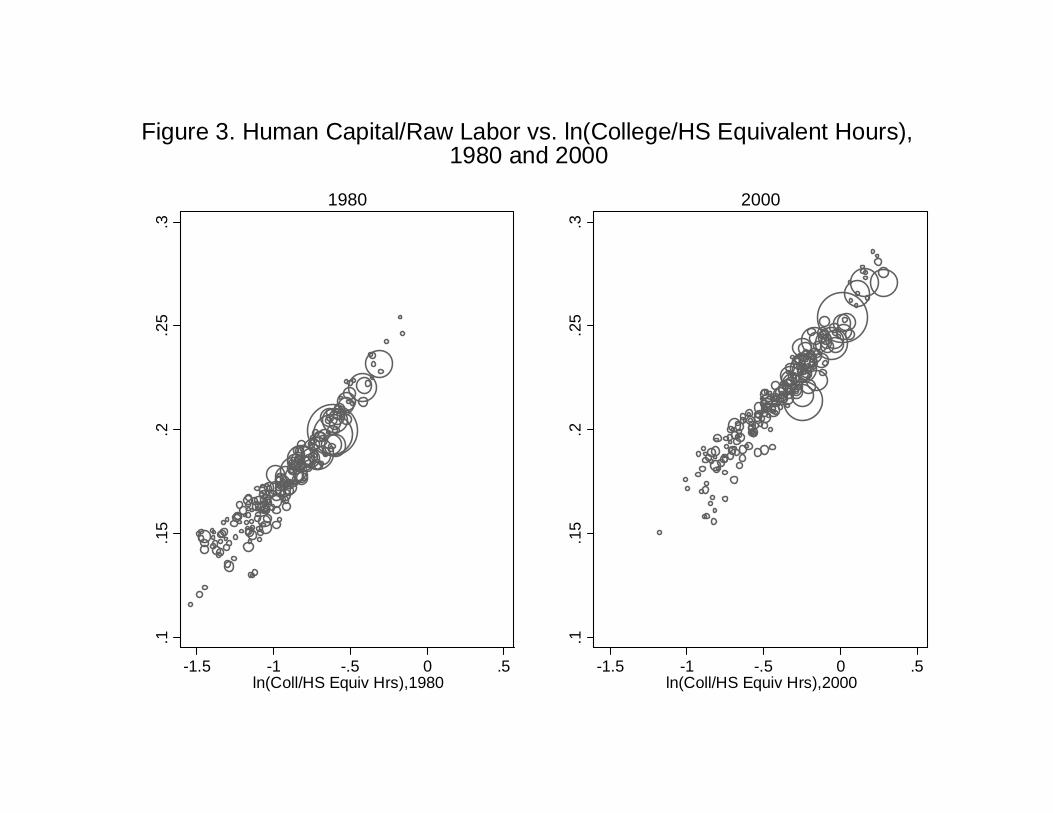
.1.1

5.2

.25

.3

-1.5 -1 -.5 0 .5ln(Coll/HS Equiv Hrs),1980

1980

.1.1

5.2

.25

.3

-1.5 -1 -.5 0 .5ln(Coll/HS Equiv Hrs),2000

2000

Figure 3. Human Capital/Raw Labor vs. ln(College/HS Equivalent Hours),1980 and 2000

  

-.4-.2

0.2

.4.6

-.1 -.05 0 .05 .1

Education group effects (column 1)

-.4-.2

0.2

.4.6

-.1 -.05 0 .05 .1

+ industry mix (2)

-.4-.2

0.2

.4.6

-.1 -.05 0 .05 .1

+ state effects (3)

-.4-.2

0.2

.4.6

-.1 -.05 0 .05 .1

+ city controls (4)

Male-Female

-.2-.1

0.1

.2

-.1 -.05 0 .05 .1

Education group effects (column 1)

-.2-.1

0.1

.2

-.1 -.05 0 .05 .1

+ industry mix (2)

-.2-.1

0.1

.2

-.1 -.05 0 .05 .1

+ state effects (3)

-.2-.1

0.1

.2

-.1 -.05 0 .05 .1

+ city controls (4)

College-High School

Figure 4. Residual Plots: Change in Wage Gaps, 1980-2000vs. 1980 Human Capital/Raw Labor

  

BostonBostonBostonBostonBoston

CharlotteCharlotteCharlotteCharlotteCharlotte

ChicagoChicagoChicagoChicagoChicago

DenverDenverDenverDenverDenver

El PasoEl PasoEl PasoEl PasoEl Paso Fresno, CAFresno, CAFresno, CAFresno, CAFresno, CA

Hickory, NCHickory, NCHickory, NCHickory, NCHickory, NC

HonoluluHonoluluHonoluluHonoluluHonolulu

HoustonHoustonHoustonHoustonHouston

Las VegasLas VegasLas VegasLas VegasLas Vegas Los AngelesLos AngelesLos AngelesLos AngelesLos Angeles

MinneapolisMinneapolisMinneapolisMinneapolisMinneapolisNYCNYCNYCNYCNYC

St. LouisSt. LouisSt. LouisSt. LouisSt. Louis

SF Bay AreaSF Bay AreaSF Bay AreaSF Bay AreaSF Bay Area

Scranton, PAScranton, PAScranton, PAScranton, PAScranton, PA

SeattleSeattleSeattleSeattleSeattleDCDCDCDCDC

.3.4

.5.6

.7A

djus

ted

PC

s pe

r wor

ker,

2000

.1 .15 .2 .25Human Capital/Raw Labor, 1980

Figure 5. 2000 Adjusted* PCs/Worker vs. 1980 Human Capital/Raw Labor

*Adjusted for Size x Industry

  

Mean Stand Dev Mean Stand Dev Mean Stand Dev(1) (2) (3) (4) (5) (6)

Adjusted Male-Female Wage GapAll Education Levels 0.376 0.098 0.254 0.054 -0.123 0.082 High School Dropouts 0.461 0.075 0.261 0.054 -0.200 0.068 High School Graduates 0.445 0.063 0.283 0.054 -0.162 0.041 >0 and <4 years college 0.380 0.053 0.248 0.047 -0.132 0.038 4 Years College 0.337 0.055 0.236 0.048 -0.102 0.052 Advanced Degree 0.257 0.068 0.239 0.054 -0.018 0.067

Adjusted College-HS Wage Gap 0.257 0.045 0.449 0.046 0.192 0.046Human Capital/Raw Labor 0.188 0.021 0.231 0.023 0.043 0.014Adjusted PCs/Worker 0.497 0.055

Number of Metro Areas

1980 2000 Change 1980-2000

Table 1. Descriptive Statistics

Notes: Raw data sources are the 1980 (Ruggles et al., 2010) and 2000 public use 5% censuses of population for the w age and human capital variables, and 2000 and 2002 surveys by Harte Hanks for PCs per w orker, both of w hich have been collapsed (using sample w eights for Census variables) to a metropolitan area-average level dataset w hose descriptive statistics are show n in this table. Sample used to compute human capital/raw labor consists of w orkers age 16-65 w ith positive potential w ork experience (age - years of education -6) and hours w orked last year, and not residing in group quarters. This variable is close to an hours-w eighted average years of schooling above 10 years (multiplied by the estimated return to schooling in 1980, 0.077), w ith an adjustment for the share of hours w orked by females -- see text for details. Wage sample further limited to those w ho are currently employed, w ith positive w age earnings but zero business and farm earnings and not currently enrolled in school. Wage adjusted, separately by gender and education (and year), for a quartic in potential experience, linear returns to education (for high school dropouts, some college, and advanced degree categories) and dummies for foreign-born, black, Hispanic, and being born after 1950. (The latter is also interacted w ith years education for the same three groups). PCs per w orker are regression adjusted for 3 digit industry x employer size dummies. The descriptive statistics in this table are w eighted by1980 population.

230 230 230

  

(1) (2) (3) (4) (5) (6) (7) (8)

Adj Coll-HS Wage -0.231 -0.128 -0.163 -0.141 -0.207 -0.167 -0.151 Gap, 1980-2000 (0.059) (0.049) (0.047) (0.046) (0.057) (0.053) (0.054)4 x Adj (linear) Return -0.149 to Schl, 1980-2000 (0.080)Intercept -0.078 -0.098 -0.066 -0.095 -0.083 -0.091 -0.094 -0.114

(0.012) (0.009) (0.009) (0.009) (0.011) (0.010) (0.010) (0.005)

Root MSE 0.054 0.052 0.046 0.051 0.050 0.049 0.049 0.049R-squared 0.577 0.613 0.491 0.617 0.655 0.660 0.664 0.662Observations 1,150 1,150 1,150 1,150 1,150 1,150 1,150 1,150ControlsEducation Group? Y Y Y Y Y Y Y YIndustry Mix N 2 Manuf Detailed 2 Manuf 2 Manuf 2 Manuf 2 Manuf 2 Manuf x Broad Education?1 (Individual) +Index +Index +Index +Index +IndexState Effects? N N N N Y Y Y YCity Controls?2 N N N N N Y Y YF Emp Rate x Broad Ed?3 N N N N N N Y Y

Table 2. Change in Male-Female Wage Gaps vs. Change in Schooling Wage Gaps, 1980-2000, Estimated by OLS

Data Source: 5% Public-use 1980 (Ruggles et al., 2010) and 2000 public use censuses of population, w hich are aggregated to 230 metropolitan areas, and, for the dependent variable, x 5 education groups (high school dropouts, graduates, some college <4 years, 4 years college, and advanced degree) that are the units of observation in the regressions. Sample consists of w orkers age 16-65 w ith positive potential w ork experience (age - years of education -6) and hours w orked last year, not residing in group quarters,w ho are currently employed, w ith positive w age earnings but zero business and farm earnings and not currently enrolled in school. Dependent variable is the gap betw een the average ln hourly w age of men and w omen w ith the same broad education level, adjusted in gender x education (x year) specif ic regressions for a quartic in potential experience, linear education (for dropouts, some college, and advanced degree) and dummies for black, Hispanic, foreign-born, and born after 1950 (w ith latter also interacted w ith years education for the same three groups). Independent variable is the average of (simililarly adjusted) college-high school w age gaps for men and w omen. All regressions in table w eighted by 1980 population. Standard errors, in parentheses under slope estimates, are computed to be robust to arbitrary forms of heteroskedasticity and error correlation w ithin metropolitan area. 1Columns (2) and (4)-(8) control for the share of employment in non-durable and durable manufacturing their interactions w ith a dummy for being in the "some college" or low er broad education group. Column (3) adds to the indvidual-level w age adjustments controls for detailed census of population industries that corresponds roughly to the level of industry detail in 1980. Columns (4) and higher control for a female demand "Index" w hich is the female share of employment obtained by averaging national female employment shares by detailed industry using local employment by industry as w eights. This index is constructed separately for "college equivalents" (w hich is is used as the control for broad education categories four years college and advanced degrees) and "high school equivalents" (w hich is is used as the control for broad education categories dropouts, high school and some college) but entered as a single control variable. 2City controls are share black, Hispanic, and foreign-born; and the unemployment rate and the natural log of the labor force. 3Female employment rates entered separately for those w ith some college or less and four years college or more.

  

(1) (2) (3) (4) (5)

Human Capital/ -0.528 -0.804 -0.891 -1.048 -0.932 Raw Labor, 1980 (0.142) (0.177) (0.252) (0.316) (0.315)

R-squared 0.578 0.630 0.661 0.666 0.667

Human Capital/ 0.993 1.248 1.258 1.267 1.287 Raw Labor, 1980 (0.276) (0.381) (0.289) (0.351) (0.389)

R-squared 0.207 0.274 0.588 0.603 0.604Observations 1,150 1,150 1,150 1,150 1,150ControlsEducation Group? Y Y Y Y YIndustry Mix N 2 Manuf 2 Manuf 2 Manuf 2 Manuf x Broad Education?1 +Index +Index +Index +IndexState Effects? N N Y Y YCity Controls?2 N N N Y YF Emp Rate x Broad Ed?3 N N N N Y

Table 3. Change in Wage Gaps on Human Capital/Raw Labor, 1980

A. Change in Adjusted Male-Female Wage Gap, 1980-2000

B. Change in Adjusted College-High School Wage Gap, 1980-2000

Data Source: 5% Public-use 1980 (Ruggles et al., 2010) and 2000 Censuses of Population, w hich are aggregated to 230 metropolitan areas (and, for the dependent variable in panel A, x 5 education groups -- high school dropouts, graduates, some college <4 years, 4 years college, and advanced degree). Sample for constructing independent variable consists of w orkers age 16-65 w ith positive potential w ork experience (age - years of education -6) and hours w orked last year, not residing in group quarters. "Human capital" is the sum of the interaction of hours w orked w ith years of education beyond 10 times 0.077, and "raw labor" is 1.423 times the sum of male hours w orked plus the sum of female hours w orked. The w age sample is the subsample w ho are currently employed, w ith positive w age earnings but zero business and farm earnings and not currently enrolled in school. Dependent variable in panel A is the (change in the) gap betw een the average ln hourly w age of men and w omen w ith the same broad education level, w here the adjustment are gender x education (x year) specif ic regressions on a quartic in potential experience, linear education (for dropouts, some college, and advanced degree) and dummies for black, Hispanic, foreign-born, and born after 1950 (w ith latter also interacted w ith years education for the same three groups). Dependent variable in panel B is the average of (simililarly adjusted change in the) college-high school w age gaps for men and w omen. All regressions in table w eighted by 1980 population. Standard errors, in parentheses under slope estimates, are computed to be robust to arbitrary forms of heteroskedasticity and error correlation w ithin metropolitan area. 1Columns (2)-(5) control for the share of employment in non-durable and durable manufacturing their interactions w ith a dummy for being in the "some college" or low er broad education group, and for a female demand "Index" w hich is the female share of employment obtained by averaging national female employment shares by detailed industry using local employment by industry as w eights. This index is constructed separately for "college equivalents" (w hich is is used as the control for broad education categories four years college and advanced degrees) and "high school equivalents" (w hich is is used as the control for broad education categories dropouts, high school and some college) but entered as a single control variable. 2City controls are share black, Hispanic, and foreign-born; and the unemployment rate and the natural log of the labor force. 3Female employment rates entered separately for those w ith some college or less and four years college or more.

  

(1) (2) (3) (4) (5)

Personal Computers/ -0.204 -0.207 -0.157 -0.115 -0.089 Worker, 2000 (0.048) (0.041) (0.052) (0.061) (0.066)Change in Hum Cap/ 0.821 0.417 0.032 -0.192 -0.355 RL, 1980-2000 (0.180) (0.172) (0.338) (0.365) (0.408)

Root MSE 0.053 0.051 0.050 0.049 0.049R-squared 0.591 0.626 0.654 0.659 0.663

Personal Computers/ -0.239 -0.363 -0.367 -0.482 -0.440 Worker, 2000 (0.063) (0.081) (0.095) (0.152) (0.158)Change in Hum Cap/ 0.845 0.547 0.589 0.371 0.178 RL, 1980-2000 (0.188) (0.203) (0.367) (0.466) (0.479)

Root MSE 0.053 0.051 0.050 0.051 0.050Observations 1,150 1,150 1,150 1,150 1,150

First Stage F-Stat 136.5 107.9 93.8 74.1 63.1 p-value 0.000 0.000 0.000 0.000 0.000

ControlsEducation Group? Y Y Y Y YIndustry Mix N 2 Manuf 2 Manuf 2 Manuf 2 Manuf x Broad Education?1 +Index +Index +Index +IndexState Effects? N N Y Y YCity Controls?2 N N N Y YF Emp Rate x Broad Ed?3 N N N N Y

Table 4a. Change in (Adjusted) Male-Female Wage Gaps, 1980-2000, vs. Personal Computer Adoption Intensity

Data Source: Dependent variable and human capital -- 5% Public-use 1980(Ruggles et al., 2010) and 2000 Censuses of Population, w hich are aggregated to 230 metropolitan areas, and, for the dependent variable, x 5 education groups (high school dropouts, graduates, some college <4 years, 4 years college, and advanced degree) that are the units of observation in the regressions. Sample used to compute human capital/raw labor, consists of w orkers age 16-65 w ith positive potential w ork experience (age - years of education -6) and hours w orked last year, and not residing in group quarters. "Human capital" is the sum of the interaction of hours w orked w ith years of education beyond 10 times 0.077, and "raw labor" is 1.423 times the sum of male hours w orked plus the sum of female hours w orked. The w age sample is the subsample w ho are currently employed, w ith positive w age earnings but zero business and farm earnings and not currently enrolled in school; dependent variable is the change in the adjusted w age gap betw een the average ln hourly w age of men and w omen w ith the same broad education level, w here the adjustment are gender x education (x year) specif ic regressions on a quartic in potential experience, linear education (for dropouts, some college, and advanced degree) and dummies for black, Hispanic, foreign-born, and born after 1950 (w ith latter also interacted w ith years education for the same three groups). PCs per w orker computed from stacked 2000 and 2002 marketing surveys by Harte Hanks, w hich are regression adjusted for 3 digit industry x employer size dummies. Instrument is 1980 human capital/raw labor. All regressions in table w eighted by 1980 population. Standard errors, in parentheses under slope estimates, are computed to be robust to arbitrary forms of heteroskedasticity and error correlation w ithin metropolitan area. 1Columns (2)-(5) control for the share of employment in non-durable and durable manufacturing their interactions w ith a dummy for being in the "some college" or low er broad education group, and for a female demand "Index" w hich is the female share of employment obtained by averaging national female employment shares by detailed industry using local employment by industry as w eights. This index is constructed separately for "college equivalents" (w hich is is used as the control for broad education categories four years college and advanced degrees) and "high school equivalents" (w hich is is used as the control for broad education categories dropouts, high school and some college) but entered as a single control variable. 2City controls are share black, Hispanic, and foreign-born; and the unemployment rate and the natural log of the labor force. 3Female employment rates entered separately for those w ith some college or less and four years college or more.

A. Ordinary Least Squares

B. Instrumental Variables

  

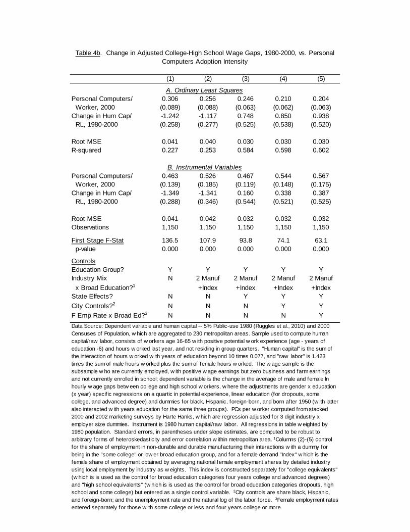
(1) (2) (3) (4) (5)

Personal Computers/ 0.306 0.256 0.246 0.210 0.204 Worker, 2000 (0.089) (0.088) (0.063) (0.062) (0.063)Change in Hum Cap/ -1.242 -1.117 0.748 0.850 0.938 RL, 1980-2000 (0.258) (0.277) (0.525) (0.538) (0.520)

Root MSE 0.041 0.040 0.030 0.030 0.030R-squared 0.227 0.253 0.584 0.598 0.602

Personal Computers/ 0.463 0.526 0.467 0.544 0.567 Worker, 2000 (0.139) (0.185) (0.119) (0.148) (0.175)Change in Hum Cap/ -1.349 -1.341 0.160 0.338 0.387 RL, 1980-2000 (0.288) (0.346) (0.544) (0.521) (0.525)

Root MSE 0.041 0.042 0.032 0.032 0.032Observations 1,150 1,150 1,150 1,150 1,150

First Stage F-Stat 136.5 107.9 93.8 74.1 63.1 p-value 0.000 0.000 0.000 0.000 0.000

ControlsEducation Group? Y Y Y Y YIndustry Mix N 2 Manuf 2 Manuf 2 Manuf 2 Manuf x Broad Education?1 +Index +Index +Index +IndexState Effects? N N Y Y YCity Controls?2 N N N Y YF Emp Rate x Broad Ed?3 N N N N Y

Table 4b. Change in Adjusted College-High School Wage Gaps, 1980-2000, vs. Personal Computers Adoption Intensity

B. Instrumental Variables

A. Ordinary Least Squares

Data Source: Dependent variable and human capital -- 5% Public-use 1980 (Ruggles et al., 2010) and 2000 Censuses of Population, w hich are aggregated to 230 metropolitan areas. Sample used to compute human capital/raw labor, consists of w orkers age 16-65 w ith positive potential w ork experience (age - years of education -6) and hours w orked last year, and not residing in group quarters. "Human capital" is the sum of the interaction of hours w orked w ith years of education beyond 10 times 0.077, and "raw labor" is 1.423 times the sum of male hours w orked plus the sum of female hours w orked. The w age sample is the subsample w ho are currently employed, w ith positive w age earnings but zero business and farm earnings and not currently enrolled in school; dependent variable is the change in the average of male and female ln hourly w age gaps betw een college and high school w orkers, w here the adjustments are gender x education (x year) specif ic regressions on a quartic in potential experience, linear education (for dropouts, some college, and advanced degree) and dummies for black, Hispanic, foreign-born, and born after 1950 (w ith latter also interacted w ith years education for the same three groups). PCs per w orker computed from stacked 2000 and 2002 marketing surveys by Harte Hanks, w hich are regression adjusted for 3 digit industry x employer size dummies. Instrument is 1980 human capital/raw labor. All regressions in table w eighted by 1980 population. Standard errors, in parentheses under slope estimates, are computed to be robust to arbitrary forms of heteroskedasticity and error correlation w ithin metropolitan area. 1Columns (2)-(5) control for the share of employment in non-durable and durable manufacturing their interactions w ith a dummy for being in the "some college" or low er broad education group, and for a female demand "Index" w hich is the female share of employment obtained by averaging national female employment shares by detailed industry using local employment by industry as w eights. This index is constructed separately for "college equivalents" (w hich is is used as the control for broad education categories four years college and advanced degrees) and "high school equivalents" (w hich is is used as the control for broad education categories dropouts, high school and some college) but entered as a single control variable. 2City controls are share black, Hispanic, and foreign-born; and the unemployment rate and the natural log of the labor force. 3Female employment rates entered separately for those w ith some college or less and four years college or more.

  

(1) (2) (3) (4) (5)

Adj Coll-HS Wage -0.532 -0.644 -0.708 -0.827 -0.724 Gap, 1980-2000 (0.206) (0.288) (0.279) (0.383) (0.365)Intercept -0.020 0.001 0.014 0.036 0.017

(0.038) (0.054) (0.053) (0.073) (0.069)

Root MSE 0.0555 0.0557 0.0523 0.0535 0.0522R-squared 0.549 0.549 0.617 0.601 0.620Observations 1,150 1,150 1,150 1,150 1,150ControlsEducation Group? Y Y Y Y YIndustry Mix N 2 Manuf 2 Manuf 2 Manuf 2 Manuf x Broad Education?1 +Index +Index +Index +IndexState Effects? N N Y Y YCity Controls?2 N N N Y YF Emp Rate x Broad Ed?3 N N N N Y

Table 5. Male-Female Wage Gaps vs. College-High School Wage Gaps, Estimated by Instrumental Variables

Data Source: 5% Public-use 1980 (Ruggles et al., 2010) and 2000 public use censuses of population, w hich are aggregated to 230 metropolitan areas, and, for the dependent variable, x 5 education groups (high school dropouts, graduates, some college <4 years, 4 years college, and advanced degree) that are the units of observation in the regressions. Sample consists of w orkers age 16-65 w ith positive potential w ork experience (age - years of education -6) and hours w orked last year, not residing in group quarters,w ho are currently employed, w ith positive w age earnings but zero business and farm earnings and not currently enrolled in school. Dependent variable is the gap (in panel A, or change in the gap, in panel B) betw een the average ln hourly w age of men and w omen w ith the same broad education level, w here the adjustment are gender x education (x year) specif ic regressions on a quartic in potential experience, linear education (for dropouts, some college, and advanced degree) and dummies for black, Hispanic, foreign-born, and born after 1950 (w ith latter also interacted w ith years education for the same three groups). Independent variable is the average of (simililarly adjusted) college-high school w age gaps for men and w omen. The instrument is 1980 "human capital/raw labor"; f irst stage and further description of this variable are found in the notes to tables 3a and 4a. All regressions in table w eighted by 1980 population. Standard errors, in parentheses under slope estimates, are computed to be robust to arbitrary forms of heteroskedasticity and error correlation w ithin metropolitan area. 1Columns (2)-(5) control for the share of employment in non-durable and durable manufacturing their interactions w ith a dummy for being in the "some college" or low er broad education group, and for a female demand "Index" w hich is the female share of employment obtained by averaging national female employment shares by detailed industry using local employment by industry as w eights. This index is constructed separately for "college equivalents" (w hich is is used as the control for broad education categories four years college and advanced degrees) and "high school equivalents" (w hich is is used as the control for broad education categories dropouts, high school and some college) but entered as a single control variable. 2City controls are share black, Hispanic, and foreign-born; and the unemployment rate and the natural log of the labor force. 3Female employment rates entered separately for those w ith some college or less and four years college or more.

  

Predicted NatBn,Non-Emp. Rates Hs Whites Estimated Estimated

High1 w/no kids<6 Nationally By MSA(1) (2) (3) (4) (5)

Adj Coll-HS Wage -0.150 -0.085 -0.335 -0.185 -0.354 Gap, 1980-2000 (0.070) (0.079) (0.101) (0.072) (0.318)

Root MSE 0.047 0.075 0.096 0.050 0.312R-squared 0.684 0.512 0.422 0.895 0.247

Adj Coll-HS Wage -0.610 -0.452 -0.924 -0.490 -0.884 Gap, 1980-2000 (0.317) (0.276) (0.401) (0.282) (0.775)

Root MSE 0.049 0.075 0.097 0.050 0.313Observations 795 795 795 795 795ControlsEducation Group? Y Y Y Y YIndustry Mix 2 Manuf 2 Manuf 2 Manuf 2 Manuf 2 Manuf x Broad Education?2 +Index +Index +Index +Index +IndexState Effects? Y Y Y Y YCity Controls?3 Y Y Y Y YData Source: 5% Public-use 1980 (Ruggles et al., 2010) and 2000 public use censuses of population, w hich are aggregated to 230 metropolitan areas, and, for the dependent variable, x 5 education groups (high school dropouts, graduates, some college <4 years, 4 years college, and advanced degree) that are the units of observation in the regressions. Sample consists of w orkers age 16-65 w ith positive potential w ork experience (age - years of education-6) and hours w orked last year, not residing in group quarters,w ho are currently employed, w ith positive w age earnings but zero business and farm earnings and not currently enrolled in school. Dependent variable is the gap betw een the average ln hourly w age of men and w omen w ith the same broad education level, adjusted in gender x education (x year) specif ic regressions for a quartic in potential experience, linear education (for dropouts, some college, and advanced degree) and dummies for black, Hispanic, foreign-born, and born after 1950 (w ith latter also interacted w ith years education for the same three groups). Independent variable is the average of (simililarly adjusted) college-high school w age gaps for men and w omen. All regressions in table w eighted by 1980 population. Standard errors, in parentheses under slope estimates, are computed to be robust to arbitrary forms of heteroskedasticity and error correlation w ithin metropolitan area. The instrument, used in panels B, is 1980 "human capital/raw labor," w hich is discussed in notes to previous tables. 1Women w ith characteristics associated w ith a greater than 60 chance of w orking in the average metropolitan area (as of 1980). To determine this, a probit for being in the w age sample (among w omen age 16-65 w ith positive potential w ork experience not residing in group quarters) on the same variables as the w age adjustment plus dummies for marital status interacted w ith a dummy for children under six, w as separately estimated by gender and education using the 1980 data. The predicted values, p, from this probit (evaluated at the average of the metropolitan area effects) w as computed and w omen w ith p>0.6 w ere retained. 2The share of employment in non-durable and durable manufacturing and their interactions w ith a dummy for being in the "some college" or low er broad education group, and a female demand "Index" w hich is the female share of employment obtained by averaging national female employment shares by detailed industry using local employment by industry as w eights. The index is constructed separately for "college equivalents" (w hich is is used as the control for broad education categories four years college and advanced degrees) and "high school equivalents" (w hich is is used as the control for broad education categories dropouts, high school and some college) 3City controls are share black, Hispanic, and foreign-born; and the unemployment rate and the natural log of the labor force.

Table 6. Correcting for Selection

B. Change in Adjusted Male-Female Wage Gap, 1980-2000, IV

Female Subsample

A. Change in Adjusted Male-Female Wage Gap, 1980-2000, OLS

Sel Corr: Adjusted for Inverse Mills Ratio

  

Analysis Period: 1970-1980 1980-1990 1980-2000(1) (2) (3)

Change in College-High 0.126 -0.250 -0.198 School Wage Gap (0.105) (0.061) (0.071)

R-squared 0.409 0.582 0.745

Human Capital/ -0.377 -1.380 -1.088 Raw Labor, 1980 (0.409) (0.295) (0.436)

R-squared 0.408 0.592 0.749Observations 685 685 685

Wage Methods:1 1970 1970 1980-2000

ControlsEducation Group? Y Y YIndustry Mix 2 Manuf 2 Manuf 2 Manuf x Broad Education?2 +Index +Index +IndexState Effects? Y Y YCity Controls?3 Y Y Y

Table 7. Change in Male-Female Wage Gap by Period, Large MSA subsample

Data Source: 1970 public-use "county group," 1980 5% public use, (both Ruggles et al., 2010) and 1990 and 2000 5% public use censuses of population, w hich are aggregated to 137 metropolitan areas x 5 education groups (high school dropouts, graduates, some college <4 years, 4 years college, and advanced degree) that are the units of observation in the regressions. Sample for human capital/raw labor consists of w orkers age 16-65 w ith positive potential w ork experience (age - years of education -6) and hours w orked last year, not residing in group quarters; w age sample further limited to those w ho are currently employed, w ith positive w age earnings but zero business and farm earnings and not currently enrolled in school. Dependent variable is the gap betw een the average ln hourly w age of men and w omen w ith the same broad education level, adjusted in gender x education (x year) specif ic regressions for a quartic in potential experience, linear education (for dropouts, some college, and advanced degree) and dummies for black, Hispanic, foreign-born, and born after 1950 (w ith latter also interacted w ith years education for the same three groups). Independent variable in Panel A is the average of (simililarly adjusted) college-high school w age gaps for men and w omen. Independent variable in Panels B is "human capital" -- the sum of the interaction of annual hours w orked w ith years of education beyond 10 times 0.077 -- divided by "raw labor" --- 1.423 times the sum of male annual hours w orked plus the sum of female hours w orked. All regressions in table w eighted by 1980 population. Standard errors, in parentheses under slope estimates, are computed to be robust to arbitrary forms of heteroskedasticity and error correlation w ithin metropolitan area. 1"1970" w age methods employ categorical versions of "hours last w eek" and "w eeks last year" available in the 1970 Census, interpolated to continuous hours and w eeks (using means in 1980 census data) to compute annual hours w orked. Column (3), like the other tables, uses reports of (continuous) "usual hours per w eek" and "w eeks last year" to compute annual hours w orked. 2The share of employment in non-durable and durable manufacturing and their interactions w ith a dummy for being in the "some college" or low er broad education group, and a female demand "Index" w hich is the female share of employment obtained by averaging national female employment shares by detailed industry using local employment by industry as w eights. The index is constructed separately for "college equivalents" (w hich is is used as the control for broad education categories four years college and advanced degrees) and "high school equivalents" (w hich is is used as the control for broad education categories dropouts, high school and some college) 3City controls are share black, Hispanic, and foreign-born; and the unemployment rate and the natural log of the labor force.

A. Versus Change in College-High School Wage Gap

B. Versus 1980 Human Capital/Raw Labor

  

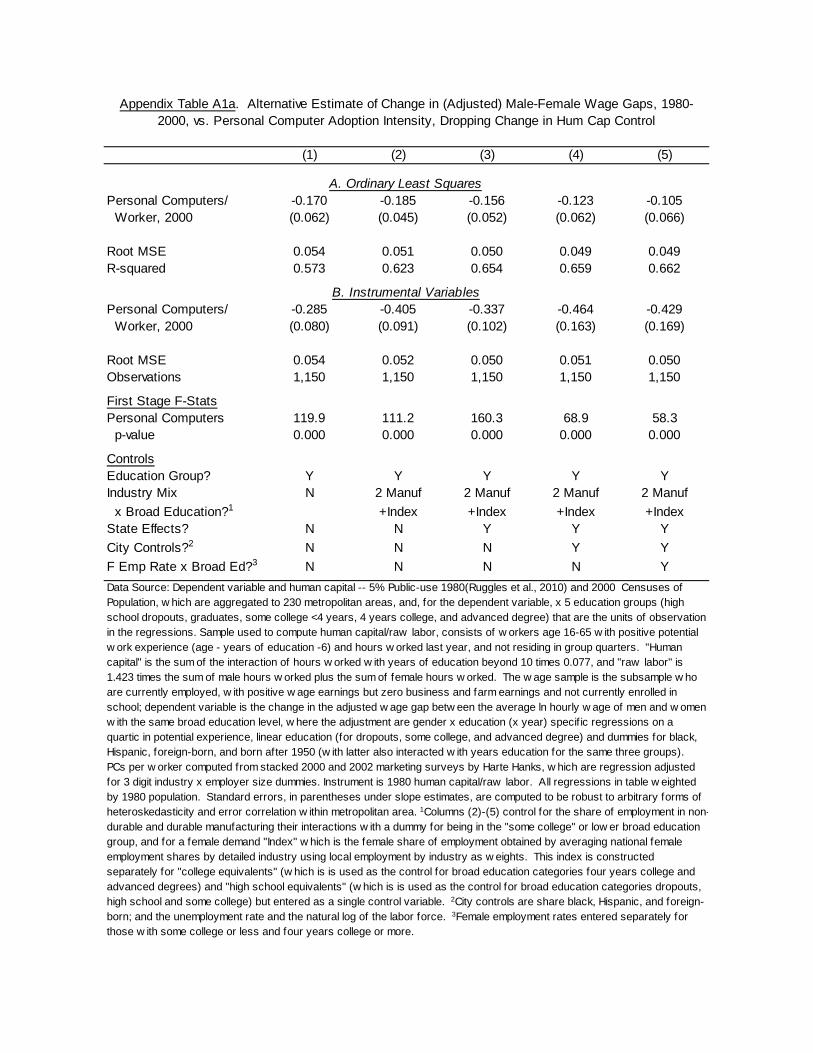
(1) (2) (3) (4) (5)

Personal Computers/ -0.170 -0.185 -0.156 -0.123 -0.105 Worker, 2000 (0.062) (0.045) (0.052) (0.062) (0.066)

Root MSE 0.054 0.051 0.050 0.049 0.049R-squared 0.573 0.623 0.654 0.659 0.662

Personal Computers/ -0.285 -0.405 -0.337 -0.464 -0.429 Worker, 2000 (0.080) (0.091) (0.102) (0.163) (0.169)

Root MSE 0.054 0.052 0.050 0.051 0.050Observations 1,150 1,150 1,150 1,150 1,150

First Stage F-StatsPersonal Computers 119.9 111.2 160.3 68.9 58.3 p-value 0.000 0.000 0.000 0.000 0.000

ControlsEducation Group? Y Y Y Y YIndustry Mix N 2 Manuf 2 Manuf 2 Manuf 2 Manuf x Broad Education?1 +Index +Index +Index +IndexState Effects? N N Y Y YCity Controls?2 N N N Y YF Emp Rate x Broad Ed?3 N N N N Y

Appendix Table A1a. Alternative Estimate of Change in (Adjusted) Male-Female Wage Gaps, 1980-2000, vs. Personal Computer Adoption Intensity, Dropping Change in Hum Cap Control

Data Source: Dependent variable and human capital -- 5% Public-use 1980(Ruggles et al., 2010) and 2000 Censuses of Population, w hich are aggregated to 230 metropolitan areas, and, for the dependent variable, x 5 education groups (high school dropouts, graduates, some college <4 years, 4 years college, and advanced degree) that are the units of observation in the regressions. Sample used to compute human capital/raw labor, consists of w orkers age 16-65 w ith positive potential w ork experience (age - years of education -6) and hours w orked last year, and not residing in group quarters. "Human capital" is the sum of the interaction of hours w orked w ith years of education beyond 10 times 0.077, and "raw labor" is 1.423 times the sum of male hours w orked plus the sum of female hours w orked. The w age sample is the subsample w ho are currently employed, w ith positive w age earnings but zero business and farm earnings and not currently enrolled in school; dependent variable is the change in the adjusted w age gap betw een the average ln hourly w age of men and w omen w ith the same broad education level, w here the adjustment are gender x education (x year) specif ic regressions on a quartic in potential experience, linear education (for dropouts, some college, and advanced degree) and dummies for black, Hispanic, foreign-born, and born after 1950 (w ith latter also interacted w ith years education for the same three groups). PCs per w orker computed from stacked 2000 and 2002 marketing surveys by Harte Hanks, w hich are regression adjusted for 3 digit industry x employer size dummies. Instrument is 1980 human capital/raw labor. All regressions in table w eighted by 1980 population. Standard errors, in parentheses under slope estimates, are computed to be robust to arbitrary forms of heteroskedasticity and error correlation w ithin metropolitan area. 1Columns (2)-(5) control for the share of employment in non-durable and durable manufacturing their interactions w ith a dummy for being in the "some college" or low er broad education group, and for a female demand "Index" w hich is the female share of employment obtained by averaging national female employment shares by detailed industry using local employment by industry as w eights. This index is constructed separately for "college equivalents" (w hich is is used as the control for broad education categories four years college and advanced degrees) and "high school equivalents" (w hich is is used as the control for broad education categories dropouts, high school and some college) but entered as a single control variable. 2City controls are share black, Hispanic, and foreign-born; and the unemployment rate and the natural log of the labor force. 3Female employment rates entered separately for those w ith some college or less and four years college or more.

A. Ordinary Least Squares

B. Instrumental Variables

  

(1) (2) (3) (4) (5)

Personal Computers/ 0.255 0.197 0.287 0.246 0.246 Worker, 2000 (0.104) (0.096) (0.063) (0.079) (0.081)

Root MSE 0.044 0.042 0.031 0.030 0.030R-squared 0.095 0.171 0.576 0.589 0.591

Personal Computers/ 0.535 0.629 0.475 0.561 0.592 Worker, 2000 (0.162) (0.206) (0.108) (0.143) (0.165)

Root MSE 0.047 0.047 0.032 0.032 0.032Observations 1,150 1,150 1,150 1,150 1,150

First Stage F-StatsPersonal Computers 119.9 111.2 160.3 68.9 58.3 p-value 0.000 0.000 0.000 0.000 0.000

ControlsEducation Group? Y Y Y Y YIndustry Mix N 2 Manuf 2 Manuf 2 Manuf 2 Manuf x Broad Education?1 +Index +Index +Index +IndexState Effects? N N Y Y YCity Controls?2 N N N Y YF Emp Rate x Broad Ed?3 N N N N Y

Appendix Table A1b. Alternative Estimates of Change in Adjusted College-High School Wage Gaps, 1980-2000, vs. Personal Computers Adoption Intensity, Dropping Change in Hum Cap Control

Data Source: Dependent variable and human capital -- 5% Public-use 1980 (Ruggles et al., 2010) and 2000 Censuses of Population, w hich are aggregated to 230 metropolitan areas. Sample used to compute human capital/raw labor, consists of w orkers age 16-65 w ith positive potential w ork experience (age - years of education -6) and hours w orked last year, and not residing in group quarters. "Human capital" is the sum of the interaction of hours w orked w ith years of education beyond 10 times 0.077, and "raw labor" is 1.423 times the sum of male hours w orked plus the sum of female hours w orked. The w age sample is the subsample w ho are currently employed, w ith positive w age earnings but zero business and farm earnings and not currently enrolled in school; dependent variable is the change in the average of male and female ln hourly w age gaps betw een college and high school w orkers, w here the adjustments are gender x education (x year) specif ic regressions on a quartic in potential experience, linear education (for dropouts, some college, and advanced degree) and dummies for black, Hispanic, foreign-born, and born after 1950 (w ith latter also interacted w ith years education for the same three groups). PCs per w orker computed from stacked 2000 and 2002 marketing surveys by Harte Hanks, w hich are regression adjusted for 3 digit industry x employer size dummies. Instruments is1980 human capital/raw labor. All regressions w eighted by 1980 population. Standard errors, in parentheses under slope estimates, are computed to be robust to arbitrary forms of heteroskedasticity and error correlation w ithin metropolitan area. 1Columns (2) and higher control for a female demand "Index" w hich is the female share of employment obtained by averaging national female employment shares by detailed industry using local employment by industry as w eights. This index is constructed separately for "college equivalents" (w hich is is used as the control for broad education categories four years college and advanced degrees) and "high school equivalents" (w hich is is used as the control for broad education categories dropouts, high school and some college) 2City controls are share black, Hispanic, and foreign-born; and the unemployment rate and the natural log of the labor force. 3Female employment rates entered separately for those w ith some college or less and four years college or more.

A. Ordinary Least Squares

B. Instrumental Variables

  

(1) (2) (3) (4) (5)

Adj Coll-HS Wage -0.668 -0.940 -0.542 -0.500 -0.425 Gap, 1980-2000 (0.279) (0.491) (0.215) (0.309) (0.310)Intercept 0.006 0.058 -0.018 -0.027 -0.041

(0.052) (0.092) (0.041) (0.059) (0.059)

Root MSE 0.057 0.062 0.051 0.050 0.050Observations 1,150 1,150 1,150 1,150 1,150ControlsEducation Group? Y Y Y Y YIndustry Mix N 2 Manuf 2 Manuf 2 Manuf 2 Manuf x Broad Education?1 +Index +Index +Index +IndexState Effects? N N Y Y YCity Controls?2 N N N Y YF Emp Rate x Broad Ed?3 N N N N Y

Appendix Table A2. Male-Female Wage Gaps vs. College-High School Wage Gaps, Estimated by Instrumental Variables (PCs/Worker as Instrument)

Data Source: 5% Public-use 1980 (Ruggles et al., 2010) and 2000 public use censuses of population, w hich are aggregated to 230 metropolitan areas, and, for the dependent variable, x 5 education groups (high school dropouts, graduates, some college <4 years, 4 years college, and advanced degree) that are the units of observation in the regressions. Sample consists of w orkers age 16-65 w ith positive potential w ork experience (age - years of education -6) and hours w orked last year, not residing in group quarters,w ho are currently employed, w ith positive w age earnings but zero business and farm earnings and not currently enrolled in school. Dependent variable is the gap (in panel A, or change in the gap, in panel B) betw een the average ln hourly w age of men and w omen w ith the same broad education level, w here the adjustment are gender x education (x year) specif ic regressions on a quartic in potential experience, linear education (for dropouts, some college, and advanced degree) and dummies for black, Hispanic, foreign-born, and born after 1950 (w ith latter also interacted w ith years education for the same three groups). Independent variable is the average of (simililarly adjusted) college-high school w age gaps for men and w omen. The instrument is 2000 adjusted PCs/w orker. Standard errors, in parentheses under slope estimates, are computed to be robust to arbitrary forms of heteroskedasticity and error correlation w ithin metropolitan area. 1Columns (2)-(5) control for the share of employment in non-durable and durable manufacturing their interactions w ith a dummy for being in the "some college" or low er broad education group, and for a female demand "Index" w hich is the female share of employment obtained by averaging national female employment shares by detailed industry using local employment by industry as w eights. This index is constructed separately for "college equivalents" (w hich is is used as the control for broad education categories four years college and advanced degrees) and "high school equivalents" (w hich is is used as the control for broad education categories dropouts, high school and some college) but entered as a single control variable. 2City controls are share black, Hispanic, and foreign-born; and the unemployment rate and the natural log of the labor force. 3Female employment rates entered separately for those w ith some college or less and four years college or more.