SketchLearn: Relieving User Burdens in ApproximateMeasurement with Automated Statistical Inference

Qun Huang†, Patrick P. C. Lee

‡, and Yungang Bao

†

†State Key Lab of Computer Architecture, Institute of Computing Technology, Chinese Academy of Sciences

‡Department of Computer Science and Engineering, The Chinese University of Hong Kong

ABSTRACTNetwork measurement is challenged to fulfill stringent re-

source requirements in the face of massive network traffic.

While approximate measurement can trade accuracy for re-

source savings, it demands intensive manual efforts to config-

ure the right resource-accuracy trade-offs in real deployment.

Such user burdens are caused by how existing approximate

measurement approaches inherently deal with resource con-

flicts when tracking massive network traffic with limited

resources. In particular, they tightly couple resource config-

urations with accuracy parameters, so as to provision suffi-

cient resources to bound the measurement errors. We design

SketchLearn, a novel sketch-based measurement framework

that resolves resource conflicts by learning their statistical

properties to eliminate conflicting traffic components. We

prototype SketchLearn on OpenVSwitch and P4, and our

testbed experiments and stress-test simulation show that

SketchLearn accurately and automatically monitors various

traffic statistics and effectively supports network-wide mea-

surement with limited resources.

CCS CONCEPTS• Networks→ Network measurement;

KEYWORDSSketch; Network measurement

ACM Reference Format:Qun Huang, Patrick P. C. Lee, and Yungang Bao. 2018. SketchLearn:

Relieving User Burdens in Approximate Measurement with Au-

tomated Statistical Inference. In SIGCOMM ’18: ACM SIGCOMM

Permission to make digital or hard copies of all or part of this work for

personal or classroom use is granted without fee provided that copies are not

made or distributed for profit or commercial advantage and that copies bear

this notice and the full citation on the first page. Copyrights for components

of this work owned by others than ACMmust be honored. Abstracting with

credit is permitted. To copy otherwise, or republish, to post on servers or to

redistribute to lists, requires prior specific permission and/or a fee. Request

permissions from permissions@acm.org.

SIGCOMM ’18, August 20–25, 2018, Budapest, Hungary© 2018 Association for Computing Machinery.

ACM ISBN 978-1-4503-5567-4/18/08. . . $15.00

https://doi.org/10.1145/3230543.3230559

2018 Conference, August 20–25, 2018, Budapest, Hungary. ACM, New

York, NY, USA, 17 pages. https://doi.org/10.1145/3230543.3230559

1 INTRODUCTIONNetwork measurement is indispensable to modern network

management in clouds and data centers. Administrators mea-

sure a variety of traffic statistics, such as per-flow frequency,

to infer the key behaviors or any unexpected patterns in op-

erational networks. They use the measured traffic statistics

to form the basis of management operations such as traffic

engineering, performance diagnosis, and intrusion preven-

tion. Unfortunately, measuring traffic statistics is non-trivial

in the face of massive network traffic and large-scale net-

work deployment. Error-free measurement requires per-flow

tracking [15], yet today’s data center networks can have

thousands of concurrent flows in a very small period from

50ms [2] down to even 5ms [56]. This would require tremen-

dous resources for performing per-flow tracking.

In view of the resource constraints, many approaches in

the literature leverage approximation techniques to trade be-

tween resource usage and measurement accuracy. Examples

include sampling [9, 37, 64], top-k counting [5, 43, 44, 46],

and sketch-based approaches [18, 33, 40, 42, 58], which we

collectively refer to as approximate measurement approaches.Their idea is to construct compact sub-linear data structures

to record traffic statistics, backed by theoretical guarantees

on how to achieve accurate measurement with limited re-

sources. Approximate measurement has formed building

blocks in many state-of-the-art network-wide measurement

systems (e.g., [32, 48, 55, 60, 62, 67]), and is also adopted in

production data centers [31, 68].

Although theoretically sound, existing approximate mea-

surement approaches are inconvenient for use. In such ap-

proaches, massive network traffic competes for the limited

resources, thereby introducing measurement errors due to

resource conflicts (e.g., multiple flows are mapped to the same

counter in sketch-based measurement). To mitigate errors,

sufficient resources must be provisioned in approximate mea-

surement based on its theoretical guarantees. Thus, thereexists a tight binding between resource configurations andaccuracy parameters. Such tight binding leads to several prac-

tical limitations (see §2.2 for details): (i) administrators need

SIGCOMM ’18, August 20–25, 2018, Budapest, Hungary Huang et al.

to specify tolerable error levels as input for resource configu-

rations; (ii) each configuration is tied to specific parameters

(e.g., thresholds); (iii) the theoretical analysis only provides

worst-case analysis and fails to guide the resource configu-

rations based on actual workloads; (iv) each configuration

is fixed for specific flow definitions; and (v) administrators

cannot readily quantify the extent of errors for measurement

results. How to bridge the gap between theoretical guaran-

tees and practical deployment in approximate measurement

remains a challenging yet critical issue [13].

We address this issue by focusing on sketch-based mea-

surement, which fully records the chosen statistics of all ob-

served packets in fixed-size data structures (i.e., sketches). We

propose SketchLearn, a sketch-based measurement frame-

work that addresses the above limitations in approximate

measurement through a fundamentally novel methodology.

Its idea is to characterize the inherent statistical properties

of resource conflicts in sketches rather than pursue a per-

fect resource configuration to mitigate resource conflicts.

Specifically, SketchLearn builds on a multi-level sketch [17]

to track the frequencies of flow records at bit-level granu-

larities. The multi-level structure leads to multiple bit-level

Gaussian distributions for the sketch counters, which we jus-

tify with rigorous theoretical analysis (see §4). SketchLearn

leverages the Gaussian distributions to address the limita-

tions of state-of-the-arts. It iteratively infers and extracts

large flows from the multi-level sketch, until the residual

multi-level sketch (with only small flows remaining) fits some

Gaussian distribution. By separating large and small flows,

SketchLearn eliminates their resource conflicts and improves

measurement accuracy. Such iterative inference can be done

without relying on complicated model parameters, thereby

relieving administrators to a large extent from configuration

burdens. SketchLearn further allows arbitrary flow defini-

tions, provides error estimates for measurement results, and

supports large-scale network-wide measurement (see §5). To

our knowledge, SketchLearn is the first approximate mea-

surement approach that builds on the characterization of the

inherent statistical properties of sketches.

We prototype SketchLearn atop OpenVSwitch [52] and

P4 [53] (see §6) to show its feasibility of being deployable

in both software and hardware switches, respectively. Our

testbed experiments and stress-test simulation show that

with only 64KB of memory and 92 CPU cycles of per-packet

processing, SketchLearn achieves near-optimal accuracy for

a variety of traffic statistics and addresses the limitations of

state-of-the-arts (see §7).

2 MOTIVATIONWe start with measuring per-flow frequencies of network traf-fic across time intervals called epochs. Each flow is identified

by a flowkey, which can be defined based on any combina-

tion of packet fields, such as 5-tuples or source-destination

address pairs. We obtain the per-flow frequencies, in terms of

packet or byte counts, for all or a subset of flows of interest

in each epoch. Based on per-flow frequencies, we can derive

sophisticated traffic statistics (see §5.1), such as heavy hitters

[43], heavy changers [17], superspreaders and DDoS [19],

cardinality [66], flow size distribution [38], and entropy [30].

2.1 Design RequirementsWe first pose the design requirements for practical network

measurement deployment.

Requirement 1 (R1): Small memory usage. Networkmeasurement should limit memory usage in both hard-

ware and software deployments. For hardware devices (e.g.,

switching ASICs and NetFPGA), high memory usage aggra-

vates chip footprints and heat consumptions, thereby increas-

ing manufacturing costs. Even though modern switching

ASICs have larger SRAM (e.g., 50-100MB) [45], the available

SRAM size remains limited for per-flow tracking. Software

switches in servers [54] can leverage abundant server-side

DRAM. However, high memory usage not only depletes the

memory of co-located applications (e.g., VMs or contain-

ers), but also degrades their performance due to more severe

cache contentions [27].

Requirement 2 (R2): Fast per-packet processing. Net-work measurement must process numerous packets at high

speed. For example, a fully utilized 10Gbps link corresponds

to a packet rate of 14.88Mpps for 64-byte packets; equiva-

lently, the time budget for each packet is only around 200

CPU cycles in a 3GHz processor. As the packet buffer size is

limited, any packet that significantly exceeds the time budget

can cause subsequent packets to be dropped.

Requirement 3 (R3): Real-time response. Somemeasure-

ment tasks, such as anomaly detection, necessitate real-

time statistics to respond quickly to potentially catastrophic

events. Lightweight measurement solutions are more pre-

ferred to avoid unexpected delays [20, 57].

Requirement 4 (R4): Generality. Designing and deploy-

ing specific solutions for each type of traffic statistics is in-

effective and also requires sophisticated resource allocation

across different solutions to provide accuracy guarantees

[47, 48]. Instead, a practical measurement solution should be

applicable to general types of traffic statistics [40, 41].

Also, resource requirements vary between hardware and

software. For example, ASIC switches have high throughput

but limited memory (see R1); in contrast, commodity hosts

generally have sufficient memory but limited CPU process-

ing power (see R2). Enabling unified measurement for both

software and hardware platforms is critical.

SIGCOMM ’18, August 20–25, 2018, Budapest, Hungary

0

25

50

75

100

MG FP Del Rev FR UM

Pre

cis

ion

(%

) Threshold=0.5% Threshold=0.1%

0

25

50

75

100

MG FP Del Rev FR UM

Re

ca

ll (%

)

Threshold=0.5% Threshold=0.1%

(a) Precision (b) Recall

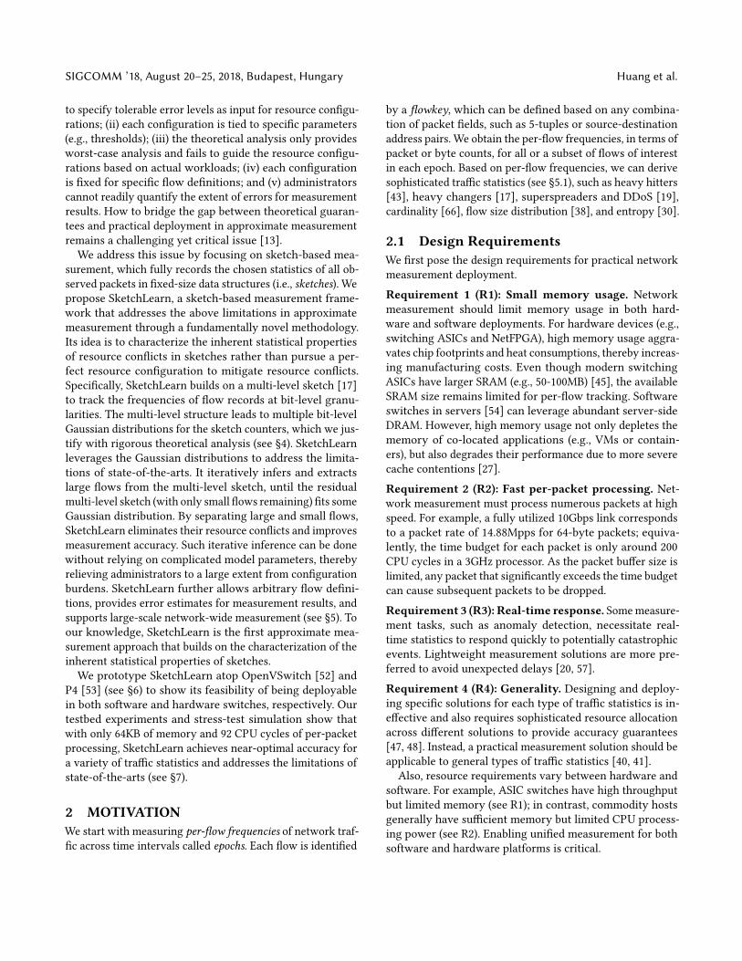
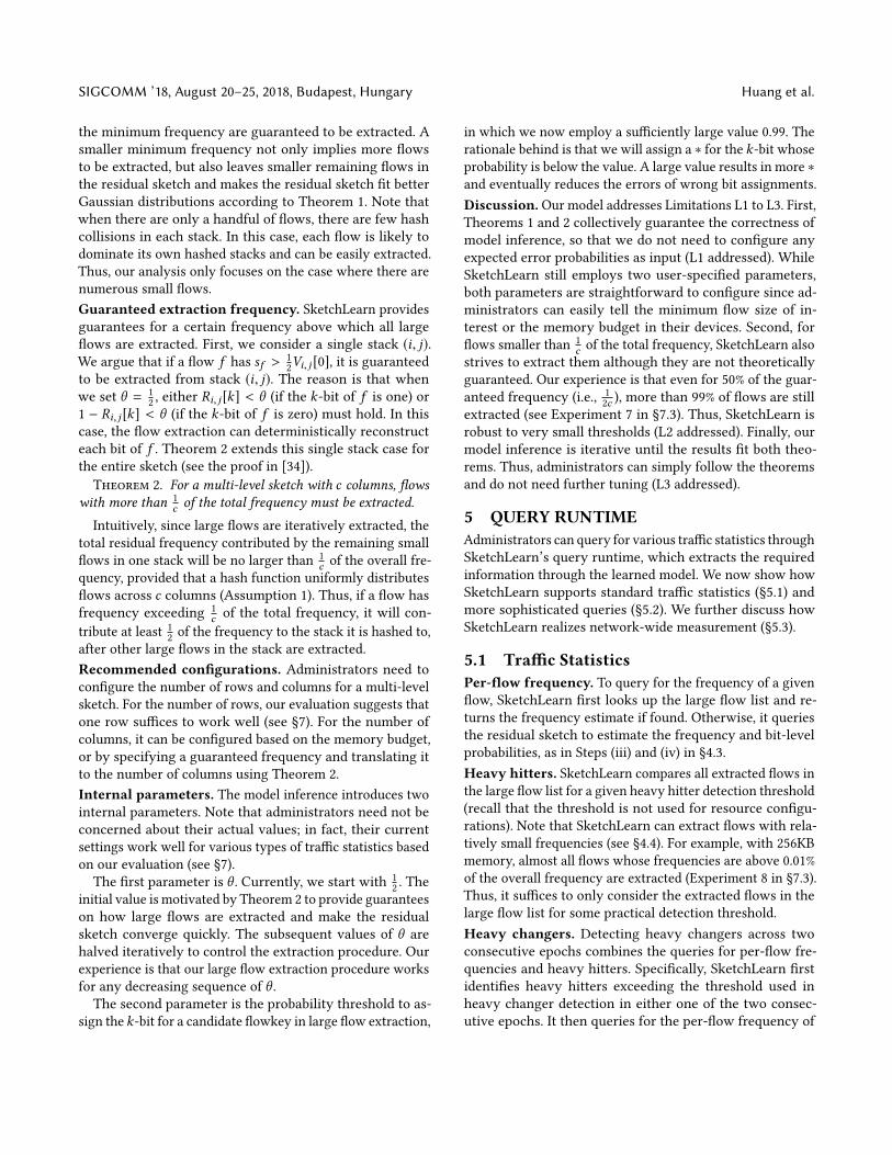
Figure 1: (L2) Accuracy with smaller thresholds.

2.2 Limitations of Existing ApproachesApproximate measurement makes design trade-offs between

resource usage and measurement accuracy (see §1). However,

existing approximate measurement approaches (including

sampling, top-k counting, and sketch-based approaches) still

fail to address the following limitations.

Limitation 1 (L1): Hard to specify expected errors. Ex-isting approximate measurement approaches mostly provide

theoretical guarantees that the estimated result has a relative

error ϵ with a confidence probability 1 − δ , where ϵ and δare configurable parameters between 0 and 1. How to pa-

rameterize the “best” ϵ and δ requires domain knowledge

for different scenarios.

Limitation 2 (L2): Hard to query different thresholds.Some measurement tasks are threshold-based. For example,

heavy hitter detection [43] finds all flows whose frequen-

cies exceed some threshold. However, existing heavy hitter

detection approaches take the threshold as input for con-

figurations, thereby making both the theoretical analysis

and actual measurement accuracy heavily tied to the thresh-

old choice. Figure 1 shows the precision and recall for six

representative heavy hitter detection approaches (see their

details in §7). We first configure the threshold as 1% of total

frequency. Then all approaches can achieve 100% in both pre-

cision and recall (not shown in the figure). If we decrease the

threshold to 0.5% and 0.1% of total traffic without changing

the configuration, then the figure shows that the precision

and recall sharply drop to less than 80% and 20%, respectively.

Limitation 3 (L3): Hard to apply theories to tune con-figurations. Even thoughwe can precisely specify the errorsand query thresholds, it remains challenging to apply the

theoretical results for two reasons. First, some measurement

approaches (e.g., [7, 40, 58]) only provide asymptotic com-

plexity results but not closed-form parameters for configura-

tions. Second, most approximate measurement approaches

perform worst-case analysis and do not take into account

actual workloads. Some studies (e.g., [23, 44]) address heavy-

tailed traffic distribution, but they need the exact distribution

models as input and cannot readily adapt to actual network

conditions. SCREAM [48] dynamically tunes configurations

based on prior runtime behaviors, but it requires complicated

coordination of a centralized controller to collect sketch sta-

tistics and fine-tune sketch configurations.

643

22

323

22

32

8

32

81

2

25

6

13

10

72

14

84

20

75

16

2532

50

3

102

105

108

MG FP Del Rev FR UM

KB

Theory basedTuned

67

K86

8K

15

K42

9K

2.3

K

5.4

K

4.7

K

4.9

K

1.2

K

2.8

K

5.7

K

14

K

102

105

108

MG FP Del Rev FR UM

CP

U C

ycle

s

Theory basedTuned

(a) Memory (b) Peak per-packet CPU cycles

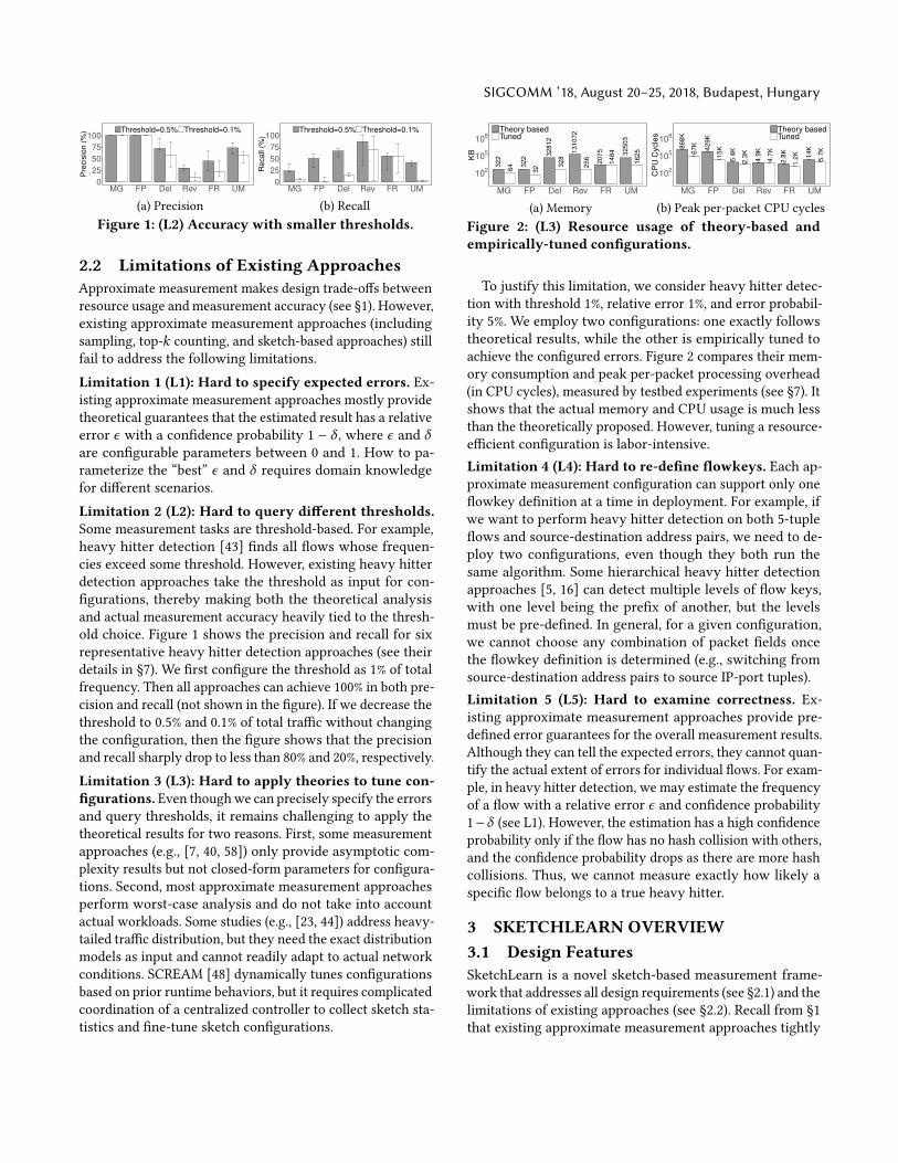
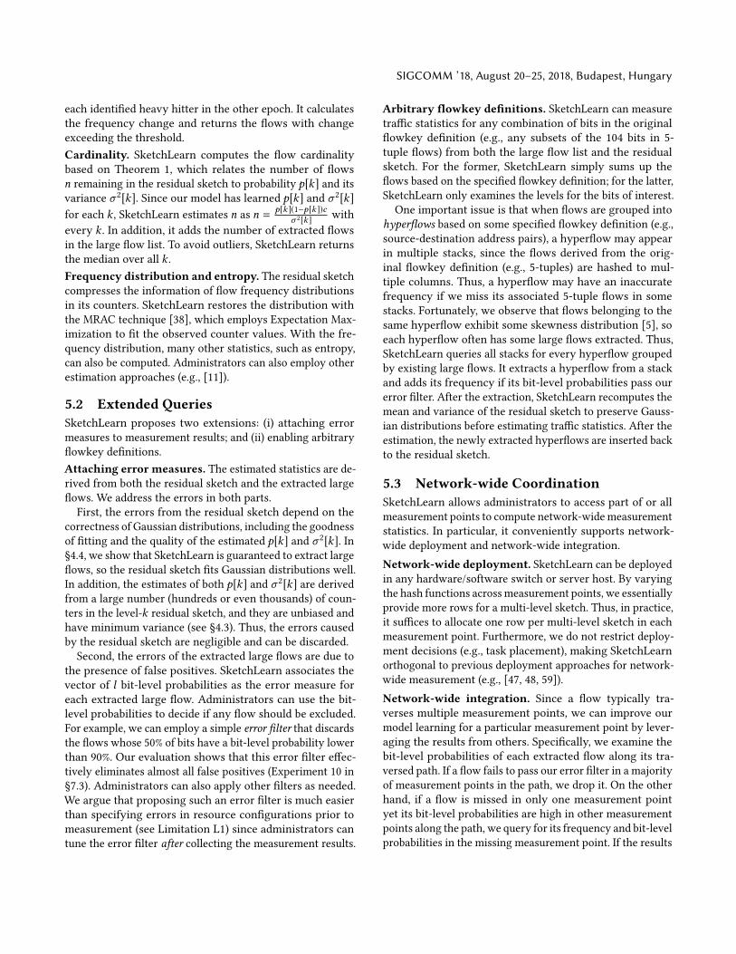
Figure 2: (L3) Resource usage of theory-based andempirically-tuned configurations.

To justify this limitation, we consider heavy hitter detec-

tion with threshold 1%, relative error 1%, and error probabil-

ity 5%. We employ two configurations: one exactly follows

theoretical results, while the other is empirically tuned to

achieve the configured errors. Figure 2 compares their mem-

ory consumption and peak per-packet processing overhead

(in CPU cycles), measured by testbed experiments (see §7). It

shows that the actual memory and CPU usage is much less

than the theoretically proposed. However, tuning a resource-

efficient configuration is labor-intensive.

Limitation 4 (L4): Hard to re-define flowkeys. Each ap-

proximate measurement configuration can support only one

flowkey definition at a time in deployment. For example, if

we want to perform heavy hitter detection on both 5-tuple

flows and source-destination address pairs, we need to de-

ploy two configurations, even though they both run the

same algorithm. Some hierarchical heavy hitter detection

approaches [5, 16] can detect multiple levels of flow keys,

with one level being the prefix of another, but the levels

must be pre-defined. In general, for a given configuration,

we cannot choose any combination of packet fields once

the flowkey definition is determined (e.g., switching from

source-destination address pairs to source IP-port tuples).

Limitation 5 (L5): Hard to examine correctness. Ex-isting approximate measurement approaches provide pre-

defined error guarantees for the overall measurement results.

Although they can tell the expected errors, they cannot quan-

tify the actual extent of errors for individual flows. For exam-

ple, in heavy hitter detection, we may estimate the frequency

of a flow with a relative error ϵ and confidence probability

1−δ (see L1). However, the estimation has a high confidence

probability only if the flow has no hash collision with others,

and the confidence probability drops as there are more hash

collisions. Thus, we cannot measure exactly how likely a

specific flow belongs to a true heavy hitter.

3 SKETCHLEARN OVERVIEW3.1 Design FeaturesSketchLearn is a novel sketch-based measurement frame-

work that addresses all design requirements (see §2.1) and the

limitations of existing approaches (see §2.2). Recall from §1

that existing approximate measurement approaches tightly

SIGCOMM ’18, August 20–25, 2018, Budapest, Hungary Huang et al.

bind resource configurations and accuracy parameters in

their designs. In sketch-based measurement, it allocates a

sketch in the form of a fixed matrix of counters, followed

by hashing packet or byte counts to each row of counters.

The sketch size (and hence the resource usage) is configured

by the input of accuracy parameters, in which the errors

are caused by hash collisions (i.e., the resource conflicts for

tracking all packets in a fixed number of counters). Existing

sketch-based measurement approaches focus on how to pre-

allocate the minimum required sketch size so as to satisfy

the accuracy requirement. In contrast, SketchLearn takes

a fundamentally new approach, in which it characterizes

and filters the impact of hash collisions through statistical

modeling. It does not need to fine-tune its configuration for

specific measurement tasks or requirements (e.g., expected

errors, query thresholds, or flow definitions). Instead, it is

self-adaptive, via statistical modeling, to various measure-

ment tasks and requirements with a single configuration. It

comprises the following design features, which address the

design requirements R1-R4 and the limitations L1-L5.

Multi-level sketch for per-bit tracking (§3.2 and §5.2).SketchLearn borrows the idea from Deltoid [17], and main-

tains amulti-level sketch composed ofmultiple small sketches,

each of which tracks the traffic statistics of a specific bit for

a given flowkey definition. Combined with statistical model-

ing, SketchLearn not only reduces the sketch size and hence

resource usage (R1-R3), but also enables flexible flowkey

definitions (L4 addressed). In the multi-level sketch, each

flowkey is composed of all candidate fields of interest (e.g.,

5-tuples), and we can extract the traffic statistics for any

combination of the packet fields by examining the levels for

the corresponding bits.

SketchLearn differs from Deltoid by extracting flowkeys

via statistical modeling. In contrast, Deltoid is tailored for

heavy hitter/changer detection based on deterministic group

testing, which requires a large sketch size to avoid hash

collisions. Also, it cannot be readily generalized for flexible

flowkey definitions. We show that SketchLearn incurs much

less resource overhead than Deltoid (see §7).

Separation of large and small flows (§4.2 and §5.1). Themulti-level sketch provides a key property that if there is no

large flow, its counter values follow a Gaussian distribution

(see Theorem 1 in §4.2). Based on this property, SketchLearn

extracts large flows from the multi-level sketch and leaves

the residual counters for small flows to form Gaussian dis-

tributions. Such separation enables SketchLearn to resolve

hash collisions for various traffic statistics (R4). For exam-

ple, SketchLearn considers the extracted large flows only for

heavy hitter detection, but includes the residual counters

when estimating cardinality. Note that some measurement

Large Flow List

Data PlaneStatistical

Model InferenceControl Plane

Network-wide Query RuntimeQuery TrafficStatistics

Flowkey Freq. Error

Bit-Level CounterDistribution

Bit 1 Distribution

Multi-LevelSketch

Multi-LevelSketch

Multi-LevelSketch

ResidualSketch

Bit 2 Distribution... ......

Bit l Distribution

Flowkey Freq. ErrorFlowkey Freq. ErrorFlowkey Freq. Error

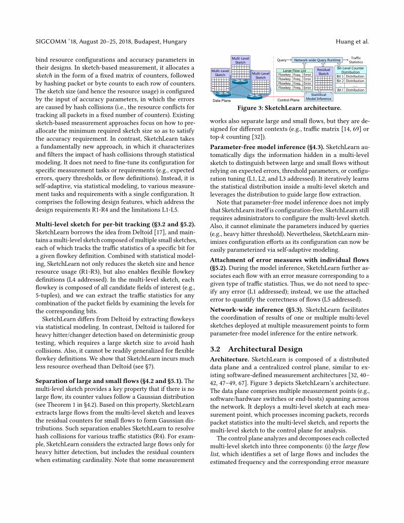
Figure 3: SketchLearn architecture.

works also separate large and small flows, but they are de-

signed for different contexts (e.g., traffic matrix [14, 69] or

top-k counting [32]).

Parameter-free model inference (§4.3). SketchLearn au-

tomatically digs the information hidden in a multi-level

sketch to distinguish between large and small flows without

relying on expected errors, threshold parameters, or configu-

ration tuning (L1, L2, and L3 addressed). It iteratively learns

the statistical distribution inside a multi-level sketch and

leverages the distribution to guide large flow extraction.

Note that parameter-free model inference does not imply

that SketchLearn itself is configuration-free. SketchLearn still

requires administrators to configure the multi-level sketch.

Also, it cannot eliminate the parameters induced by queries

(e.g., heavy hitter threshold). Nevertheless, SketchLearn min-

imizes configuration efforts as its configuration can now be

easily parameterized via self-adaptive modeling.

Attachment of error measures with individual flows(§5.2). During the model inference, SketchLearn further as-

sociates each flow with an error measure corresponding to a

given type of traffic statistics. Thus, we do not need to spec-

ify any error (L1 addressed); instead, we use the attached

error to quantify the correctness of flows (L5 addressed).

Network-wide inference (§5.3). SketchLearn facilitates

the coordination of results of one or multiple multi-level

sketches deployed at multiple measurement points to form

parameter-free model inference for the entire network.

3.2 Architectural DesignArchitecture. SketchLearn is composed of a distributed

data plane and a centralized control plane, similar to ex-

isting software-defined measurement architectures [32, 40–

42, 47–49, 67]. Figure 3 depicts SketchLearn’s architecture.

The data plane comprises multiple measurement points (e.g.,

software/hardware switches or end-hosts) spanning across

the network. It deploys a multi-level sketch at each mea-

surement point, which processes incoming packets, records

packet statistics into the multi-level sketch, and reports the

multi-level sketch to the control plane for analysis.

The control plane analyzes and decomposes each collected

multi-level sketch into three components: (i) the large flowlist, which identifies a set of large flows and includes the

estimated frequency and the corresponding error measure

SIGCOMM ’18, August 20–25, 2018, Budapest, Hungary

Flowkey: 0101

Level 4

Bit 1: 0 Bit 2: 1 Bit 3: 0 Bit 4: 1

++

Hash Value: 2 ++

++

Level 3Level 2Level 1Level 0Hash Value: 4

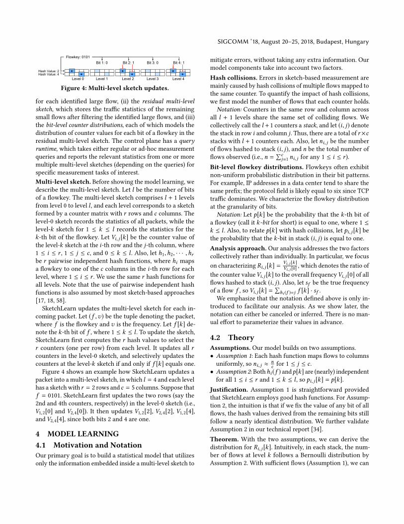
Figure 4: Multi-level sketch updates.

for each identified large flow, (ii) the residual multi-levelsketch, which stores the traffic statistics of the remaining

small flows after filtering the identified large flows, and (iii)

the bit-level counter distributions, each of which models the

distribution of counter values for each bit of a flowkey in the

residual multi-level sketch. The control plane has a queryruntime, which takes either regular or ad-hoc measurement

queries and reports the relevant statistics from one or more

multiple multi-level sketches (depending on the queries) for

specific measurement tasks of interest.

Multi-level sketch. Before showing the model learning, we

describe the multi-level sketch. Let l be the number of bits

of a flowkey. The multi-level sketch comprises l + 1 levelsfrom level 0 to level l , and each level corresponds to a sketch

formed by a counter matrix with r rows and c columns. The

level-0 sketch records the statistics of all packets, while the

level-k sketch for 1 ≤ k ≤ l records the statistics for the

k-th bit of the flowkey. Let Vi, j [k] be the counter value ofthe level-k sketch at the i-th row and the j-th column, where

1 ≤ i ≤ r , 1 ≤ j ≤ c , and 0 ≤ k ≤ l . Also, let h1,h2, · · · ,hrbe r pairwise independent hash functions, where hi maps

a flowkey to one of the c columns in the i-th row for each

level, where 1 ≤ i ≤ r . We use the same r hash functions for

all levels. Note that the use of pairwise independent hash

functions is also assumed by most sketch-based approaches

[17, 18, 58].

SketchLearn updates the multi-level sketch for each in-

coming packet. Let (f ,v) be the tuple denoting the packet,where f is the flowkey and v is the frequency. Let f [k] de-note the k-th bit of f , where 1 ≤ k ≤ l . To update the sketch,SketchLearn first computes the r hash values to select the

r counters (one per row) from each level. It updates all rcounters in the level-0 sketch, and selectively updates the

counters at the level-k sketch if and only if f [k] equals one.Figure 4 shows an example how SketchLearn updates a

packet into a multi-level sketch, in which l = 4 and each level

has a sketch with r = 2 rows and c = 5 columns. Suppose that

f = 0101. SketchLearn first updates the two rows (say the

2nd and 4th counters, respectively) in the level-0 sketch (i.e.,

V1,2[0] and V2,4[0]). It then updates V1,2[2], V2,4[2], V1,2[4],and V2,4[4], since both bits 2 and 4 are one.

4 MODEL LEARNING4.1 Motivation and NotationOur primary goal is to build a statistical model that utilizes

only the information embedded inside a multi-level sketch to

mitigate errors, without taking any extra information. Our

model components take into account two factors.

Hash collisions. Errors in sketch-based measurement are

mainly caused by hash collisions of multiple flows mapped to

the same counter. To quantify the impact of hash collisions,

we first model the number of flows that each counter holds.

Notation: Counters in the same row and column across

all l + 1 levels share the same set of colliding flows. We

collectively call the l + 1 counters a stack, and let (i, j) denotethe stack in row i and column j . Thus, there are a total of r ×cstacks with l + 1 counters each. Also, let ni, j be the number

of flows hashed to stack (i, j), and n be the total number of

flows observed (i.e., n =∑c

j=1 ni, j for any 1 ≤ i ≤ r ).

Bit-level flowkey distributions. Flowkeys often exhibit

non-uniform probabilistic distribution in their bit patterns.

For example, IP addresses in a data center tend to share the

same prefix; the protocol field is likely equal to six since TCP

traffic dominates. We characterize the flowkey distribution

at the granularity of bits.

Notation: Let p[k] be the probability that the k-th bit of

a flowkey (call it k-bit for short) is equal to one, where 1 ≤

k ≤ l . Also, to relate p[k] with hash collisions, let pi, j [k] bethe probability that the k-bit in stack (i, j) is equal to one.

Analysis approach. Our analysis addresses the two factorscollectively rather than individually. In particular, we focus

on characterizing Ri, j [k] =Vi, j [k ]Vi, j [0]

, which denotes the ratio of

the counter valueVi, j [k] to the overall frequencyVi, j [0] of allflows hashed to stack (i, j). Also, let sf be the true frequency

of a flow f , so Vi, j [k] =∑hi (f )=j f [k] · sf .

We emphasize that the notation defined above is only in-

troduced to facilitate our analysis. As we show later, the

notation can either be canceled or inferred. There is no man-

ual effort to parameterize their values in advance.

4.2 TheoryAssumptions. Our model builds on two assumptions.

• Assumption 1: Each hash function maps flows to columns

uniformly, so ni, j ≈nc for 1 ≤ j ≤ c .

• Assumption 2: Bothhi (f ) andp[k] are (nearly) independentfor all 1 ≤ i ≤ r and 1 ≤ k ≤ l , so pi, j [k] = p[k].

Justification. Assumption 1 is straightforward provided

that SketchLearn employs good hash functions. For Assump-

tion 2, the intuition is that if we fix the value of any bit of all

flows, the hash values derived from the remaining bits still

follow a nearly identical distribution. We further validate

Assumption 2 in our technical report [34].

Theorem. With the two assumptions, we can derive the

distribution for Ri, j [k]. Intuitively, in each stack, the num-

ber of flows at level k follows a Bernoulli distribution by

Assumption 2. With sufficient flows (Assumption 1), we can

SIGCOMM ’18, August 20–25, 2018, Budapest, Hungary Huang et al.

approximate the Bernoulli distribution as a Gaussian distri-

bution. We can map the distribution for number of flows into

the distribution for Ri, j [k] if stack (i, j) has no large flows

based on the following theorem (see the proof in [34]).

Theorem 1. For any stack (i, j) and level k , if stack (i, j) hasno large flows whose frequencies are significantly larger thanothers, Ri, j [k] follows a Gaussian distribution N (p[k],σ 2[k])with the meanp[k] and the variance σ 2[k] = p[k](1−p[k])c/n.

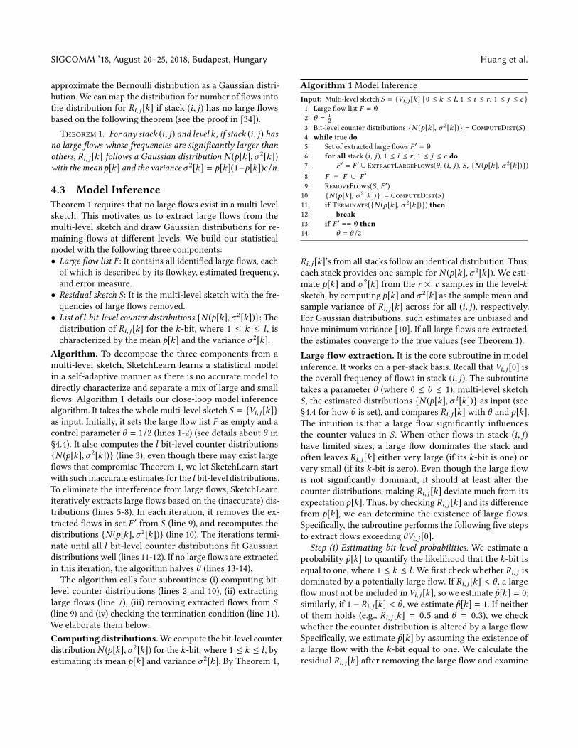
4.3 Model InferenceTheorem 1 requires that no large flows exist in a multi-level

sketch. This motivates us to extract large flows from the

multi-level sketch and draw Gaussian distributions for re-

maining flows at different levels. We build our statistical

model with the following three components:

• Large flow list F : It contains all identified large flows, each

of which is described by its flowkey, estimated frequency,

and error measure.

• Residual sketch S : It is the multi-level sketch with the fre-

quencies of large flows removed.

• List of l bit-level counter distributions {N (p[k],σ 2[k])}: Thedistribution of Ri, j [k] for the k-bit, where 1 ≤ k ≤ l , ischaracterized by the mean p[k] and the variance σ 2[k].

Algorithm. To decompose the three components from a

multi-level sketch, SketchLearn learns a statistical model

in a self-adaptive manner as there is no accurate model to

directly characterize and separate a mix of large and small

flows. Algorithm 1 details our close-loop model inference

algorithm. It takes the whole multi-level sketch S = {Vi, j [k]}as input. Initially, it sets the large flow list F as empty and a

control parameter θ = 1/2 (lines 1-2) (see details about θ in

§4.4). It also computes the l bit-level counter distributions{N (p[k],σ 2[k])} (line 3); even though there may exist large

flows that compromise Theorem 1, we let SketchLearn start

with such inaccurate estimates for the l bit-level distributions.To eliminate the interference from large flows, SketchLearn

iteratively extracts large flows based on the (inaccurate) dis-

tributions (lines 5-8). In each iteration, it removes the ex-

tracted flows in set F ′from S (line 9), and recomputes the

distributions {N (p[k],σ 2[k])} (line 10). The iterations termi-

nate until all l bit-level counter distributions fit Gaussiandistributions well (lines 11-12). If no large flows are extracted

in this iteration, the algorithm halves θ (lines 13-14).

The algorithm calls four subroutines: (i) computing bit-

level counter distributions (lines 2 and 10), (ii) extracting

large flows (line 7), (iii) removing extracted flows from S(line 9) and (iv) checking the termination condition (line 11).

We elaborate them below.

Computing distributions.We compute the bit-level counter

distribution N (p[k],σ 2[k]) for the k-bit, where 1 ≤ k ≤ l , byestimating its mean p[k] and variance σ 2[k]. By Theorem 1,

Algorithm 1Model Inference

Input: Multi-level sketch S = {Vi, j [k ] | 0 ≤ k ≤ l, 1 ≤ i ≤ r, 1 ≤ j ≤ c }1: Large flow list F = ∅

2: θ = 1

2

3: Bit-level counter distributions {N (p[k ], σ 2[k ])} = ComputeDist(S )4: while true do5: Set of extracted large flows F ′ = ∅

6: for all stack (i, j), 1 ≤ i ≤ r, 1 ≤ j ≤ c do7: F ′ = F ′ ∪ ExtractLargeFlows(θ, (i, j), S, {N (p[k ], σ 2[k ])})8: F = F ∪ F ′

9: RemoveFlows(S, F ′)

10: {N (p[k ], σ 2[k ])} = ComputeDist(S )11: if Terminate({N (p[k ], σ 2[k ])}) then12: break13: if F ′ == ∅ then14: θ = θ/2

Ri, j [k]’s from all stacks follow an identical distribution. Thus,

each stack provides one sample for N (p[k],σ 2[k]). We esti-

mate p[k] and σ 2[k] from the r × c samples in the level-ksketch, by computing p[k] and σ 2[k] as the sample mean and

sample variance of Ri, j [k] across for all (i, j), respectively.For Gaussian distributions, such estimates are unbiased and

have minimum variance [10]. If all large flows are extracted,

the estimates converge to the true values (see Theorem 1).

Large flow extraction. It is the core subroutine in model

inference. It works on a per-stack basis. Recall that Vi, j [0] isthe overall frequency of flows in stack (i, j). The subroutinetakes a parameter θ (where 0 ≤ θ ≤ 1), multi-level sketch

S , the estimated distributions {N (p[k],σ 2[k])} as input (see§4.4 for how θ is set), and compares Ri, j [k] with θ and p[k].The intuition is that a large flow significantly influences

the counter values in S . When other flows in stack (i, j)have limited sizes, a large flow dominates the stack and

often leaves Ri, j [k] either very large (if its k-bit is one) orvery small (if its k-bit is zero). Even though the large flow

is not significantly dominant, it should at least alter the

counter distributions, making Ri, j [k] deviate much from its

expectation p[k]. Thus, by checking Ri, j [k] and its differencefrom p[k], we can determine the existence of large flows.

Specifically, the subroutine performs the following five steps

to extract flows exceeding θVi, j [0].Step (i) Estimating bit-level probabilities. We estimate a

probability p̂[k] to quantify the likelihood that the k-bit isequal to one, where 1 ≤ k ≤ l . We first check whether Ri, j isdominated by a potentially large flow. If Ri, j [k] < θ , a largeflow must not be included inVi, j [k], so we estimate p̂[k] = 0;

similarly, if 1 − Ri, j [k] < θ , we estimate p̂[k] = 1. If neither

of them holds (e.g., Ri, j [k] = 0.5 and θ = 0.3), we check

whether the counter distribution is altered by a large flow.

Specifically, we estimate p̂[k] by assuming the existence of

a large flow with the k-bit equal to one. We calculate the

residual Ri, j [k] after removing the large flow and examine

SIGCOMM ’18, August 20–25, 2018, Budapest, Hungary

the difference between the residualRi, j [k] and its expectationp[k]. In particular, the difference can be converted to the

likelihood p̂[k] via Bayes’ Theorem. Our technical report

[34] presents the detailed calculation.

Step (ii) Finding candidate flowkeys. If p̂[k] or 1 − p̂[k] isclose to one (> 0.99 in our paper), the subroutine sets the k-bit as one or zero, respectively; otherwise, if neither of them

is close to one, the k-bit is assigned a wildcard bit ∗, meaning

that it can be either zero or one. We then obtain a template

flowkey composed of zero, one, and ∗. We enumerate all

candidate flows matching the template and check whether

they can be hashed to stack (i, j).Step (iii) Estimating frequencies.We estimate the frequency

for each candidate flowkey. We first produce a frequency

estimate for each k-bit using the idea of maximum likelihood

estimation. Our goal is that after excluding the contribution

of some candidate flow f , the residual Ri, j [k] is equal to its

expectation p[k]. Specifically, if we remove f , the residualoverall frequency is reduced toVi, j [0] − sf . If the k-bit is one,Vi, j [k] is also reduced to Vi, j [k] − sf ; however, if the k-bit iszero,Vi, j [k] remains unchanged after f is removed (as we do

not update the counter). Thus, by setting the residual Ri, j [k](i.e., the ratio of the residual Vi, j [k] to the residual Vi, j [0])equal to p[k], we can estimate sf as

sf =

{ Ri, j [k ]−p[k ]1−p[k] Vi, j [0], if k-bit is one,

(1 −Ri, j [k ]p[k ] )Vi, j [0], if k-bit is zero.

The final frequency estimate is taken as the median of the

estimates for all l levels of sketches to avoid outliers.

Step (iv) Associating flowkeys with bit-level probabilities.If the k-bit is equal to one (resp. zero), we associate it with

a bit-level probability p̂[k] (resp. 1 − p̂[k]). Each candidate

flowkey is accordingly associated with a vector of l bit-levelprobabilities to quantify the correctness of the flowkey. In-

tuitively, if most of the bits have high bit-level probabilities,

the candidate flowkey is more likely to correspond to a true

flowkey. In §5.2, we also show how to leverage this vector

to attach an error measure to a given flow.

Step (v) Verifying candidate flows. The subroutine may

produce false positives since there are multiple flows being

constructed by matching ∗. We filter out false positives with

the aid of other stacks. Specifically, we hash an extracted

flow with other hash functions except hi to some other stack

(i ′, j ′), where i ′ , i . We compare the current frequency

estimate using the counters in other stacks, and take the

smallest value as the final frequency estimate. Finally, we

check the final frequency estimate and remove any extracted

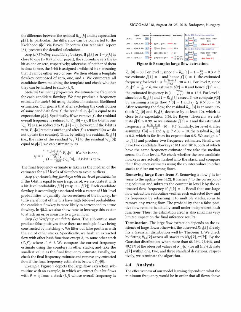
flow if the final frequency estimate is below θVi, j [0].Example. Figure 5 depicts the large flow extraction sub-

routine with an example, in which we extract four-bit flows

with θ = 1

3from a stack (i, j) whose overall frequency is

Derive p̂[4]: if removing a large flow

-2, if f[4]=12, if f[4]=0

Level 0

Level 1:

Level 2:

Level 3:

Level 4:

p̂[1]=1, f[1]=1

30

21

14

N(0.5, 0.01)

N(0.4, 0.01)

N(0.36, 0.1)

N(0.5, 0.3)

p̂[2]=0, f[2]=0

p̂[3]=0.99, f[3]=1

p̂[4]=0.38, f[4]=*

θ=1/3

12

12.5

9.7

Probability & Flowkey FrequencyInput Derive p̂[3]: if removing a large flow

Level 317 7

Level 030 20

Ratio: 17/30→7/20=0.35

Level 414 4

Level 030 20

(Close to 0.36)

Ratio: 14/30→4/20=0.20

(Far from 0.5)

7

17

Counter

Figure 5: Example: large flow extraction.

Vi, j [0] = 30. For level 1, since 1 − Ri, j [1] = 1 − 21

30= 0.3 < θ ,

we estimate p̂[1] = 1 and hence f [1] = 1; the estimated

frequency for level 1 is21/30−0.51−0.5 · 30 = 12. For level 2, since

Ri, j [2] =7

30< θ , we estimate p̂[2] = 0 and hence f [2] = 0;

the estimated frequency is (1 −7/30

0.4 ) · 30 = 12.5. For level 3,since both Ri, j [3] and 1 − Ri, j [3] exceed θ , we compute p̂[3]by assuming a large flow f [3] = 1 and sf ≥ θ × 30 = 10.

After removing the flow, the residual Ri, j [3] is at most 0.35

(both Vi, j [0] and Vi, j [3] decrease by at least 10), which is

close to its expectation 0.36. By Bayes’ Theorem, we esti-

mate p̂[3] > 0.99, so we estimate f [3] = 1 and the estimated

frequency is17/30−0.361−0.36 · 30 = 9.7. Similarly, for level 4, after

assuming f [4] = 1 and sf ≥ θ × 30 = 10, the residual Ri, j [4]is 0.2, which is far from its expectation 0.5. We assign a *

to f [4] and produce two frequency estimates. Finally, we

have two candidate flowkeys 1011 and 1010, both of which

have the same frequency estimate if we take the median

across the four levels. We check whether the two candidate

flowkeys are actually hashed into the stack, and compare

their frequency estimates using the counter values in other

stacks to filter out wrong flows.

Removing large flows from S . Removing a flow f is in-

verse to the update (see §3.2). It hashes f to the correspond-

ing columns and subtracts the counter in level k by the es-

timated flow frequency if f [k] = 1. Recall that our large

flow extraction subroutine verifies each extracted flow and

its frequency by rehashing it to multiple stacks, so as to

remove any wrong flow. The probability that a false posi-

tive flow remains is actually small under independent hash

functions. Thus, the estimation error is also small has very

limited impact on the final inference results.

Termination. The large flow extraction depends on the ex-

istence of large flows; otherwise, the observed Ri, j [k] alreadyfits a Gaussian distribution well by Theorem 1. We check

by fitting Ri, j [k] across all stacks to N (p[k],σ 2[k]). By the

Gaussian distribution, when more than 68.26%, 95.44%, and

99.73% of the observed values of Ri, j [k] (for all (i, j)) deviatep[k] within one, two, and three standard deviations, respec-

tively, we terminate the algorithm.

4.4 AnalysisThe effectiveness of our model learning depends on what the

minimum frequency would be in order that all flows above

SIGCOMM ’18, August 20–25, 2018, Budapest, Hungary Huang et al.

the minimum frequency are guaranteed to be extracted. A

smaller minimum frequency not only implies more flows

to be extracted, but also leaves smaller remaining flows in

the residual sketch and makes the residual sketch fit better

Gaussian distributions according to Theorem 1. Note that

when there are only a handful of flows, there are few hash

collisions in each stack. In this case, each flow is likely to

dominate its own hashed stacks and can be easily extracted.

Thus, our analysis only focuses on the case where there are

numerous small flows.

Guaranteed extraction frequency. SketchLearn provides

guarantees for a certain frequency above which all large

flows are extracted. First, we consider a single stack (i, j).We argue that if a flow f has sf >

1

2Vi, j [0], it is guaranteed

to be extracted from stack (i, j). The reason is that when

we set θ = 1

2, either Ri, j [k] < θ (if the k-bit of f is one) or

1 − Ri, j [k] < θ (if the k-bit of f is zero) must hold. In this

case, the flow extraction can deterministically reconstruct

each bit of f . Theorem 2 extends this single stack case for

the entire sketch (see the proof in [34]).

Theorem 2. For a multi-level sketch with c columns, flowswith more than 1

c of the total frequency must be extracted.

Intuitively, since large flows are iteratively extracted, the

total residual frequency contributed by the remaining small

flows in one stack will be no larger than1

c of the overall fre-

quency, provided that a hash function uniformly distributes

flows across c columns (Assumption 1). Thus, if a flow has

frequency exceeding1

c of the total frequency, it will con-

tribute at least1

2of the frequency to the stack it is hashed to,

after other large flows in the stack are extracted.

Recommended configurations. Administrators need to

configure the number of rows and columns for a multi-level

sketch. For the number of rows, our evaluation suggests that

one row suffices to work well (see §7). For the number of

columns, it can be configured based on the memory budget,

or by specifying a guaranteed frequency and translating it

to the number of columns using Theorem 2.

Internal parameters. The model inference introduces two

internal parameters. Note that administrators need not be

concerned about their actual values; in fact, their current

settings work well for various types of traffic statistics based

on our evaluation (see §7).

The first parameter is θ . Currently, we start with 1

2. The

initial value is motivated by Theorem 2 to provide guarantees

on how large flows are extracted and make the residual

sketch converge quickly. The subsequent values of θ are

halved iteratively to control the extraction procedure. Our

experience is that our large flow extraction procedure works

for any decreasing sequence of θ .The second parameter is the probability threshold to as-

sign the k-bit for a candidate flowkey in large flow extraction,

in which we now employ a sufficiently large value 0.99. The

rationale behind is that we will assign a ∗ for the k-bit whoseprobability is below the value. A large value results in more ∗

and eventually reduces the errors of wrong bit assignments.

Discussion. Our model addresses Limitations L1 to L3. First,

Theorems 1 and 2 collectively guarantee the correctness of

model inference, so that we do not need to configure any

expected error probabilities as input (L1 addressed). While

SketchLearn still employs two user-specified parameters,

both parameters are straightforward to configure since ad-

ministrators can easily tell the minimum flow size of in-

terest or the memory budget in their devices. Second, for

flows smaller than1

c of the total frequency, SketchLearn also

strives to extract them although they are not theoretically

guaranteed. Our experience is that even for 50% of the guar-

anteed frequency (i.e.,1

2c ), more than 99% of flows are still

extracted (see Experiment 7 in §7.3). Thus, SketchLearn is

robust to very small thresholds (L2 addressed). Finally, our

model inference is iterative until the results fit both theo-

rems. Thus, administrators can simply follow the theorems

and do not need further tuning (L3 addressed).

5 QUERY RUNTIMEAdministrators can query for various traffic statistics through

SketchLearn’s query runtime, which extracts the required

information through the learned model. We now show how

SketchLearn supports standard traffic statistics (§5.1) and

more sophisticated queries (§5.2). We further discuss how

SketchLearn realizes network-wide measurement (§5.3).

5.1 Traffic StatisticsPer-flow frequency. To query for the frequency of a given

flow, SketchLearn first looks up the large flow list and re-

turns the frequency estimate if found. Otherwise, it queries

the residual sketch to estimate the frequency and bit-level

probabilities, as in Steps (iii) and (iv) in §4.3.

Heavy hitters. SketchLearn compares all extracted flows in

the large flow list for a given heavy hitter detection threshold

(recall that the threshold is not used for resource configu-

rations). Note that SketchLearn can extract flows with rela-

tively small frequencies (see §4.4). For example, with 256KB

memory, almost all flows whose frequencies are above 0.01%

of the overall frequency are extracted (Experiment 8 in §7.3).

Thus, it suffices to only consider the extracted flows in the

large flow list for some practical detection threshold.

Heavy changers. Detecting heavy changers across two

consecutive epochs combines the queries for per-flow fre-

quencies and heavy hitters. Specifically, SketchLearn first

identifies heavy hitters exceeding the threshold used in

heavy changer detection in either one of the two consec-

utive epochs. It then queries for the per-flow frequency of

SIGCOMM ’18, August 20–25, 2018, Budapest, Hungary

each identified heavy hitter in the other epoch. It calculates

the frequency change and returns the flows with change

exceeding the threshold.

Cardinality. SketchLearn computes the flow cardinality

based on Theorem 1, which relates the number of flows

n remaining in the residual sketch to probability p[k] and its

variance σ 2[k]. Since our model has learned p[k] and σ 2[k]

for each k , SketchLearn estimates n as n =p[k ](1−p[k ])c

σ 2[k ] with

every k . In addition, it adds the number of extracted flows

in the large flow list. To avoid outliers, SketchLearn returns

the median over all k .

Frequency distribution and entropy. The residual sketchcompresses the information of flow frequency distributions

in its counters. SketchLearn restores the distribution with

the MRAC technique [38], which employs Expectation Max-

imization to fit the observed counter values. With the fre-

quency distribution, many other statistics, such as entropy,

can also be computed. Administrators can also employ other

estimation approaches (e.g., [11]).

5.2 Extended QueriesSketchLearn proposes two extensions: (i) attaching error

measures to measurement results; and (ii) enabling arbitrary

flowkey definitions.

Attaching error measures. The estimated statistics are de-

rived from both the residual sketch and the extracted large

flows. We address the errors in both parts.

First, the errors from the residual sketch depend on the

correctness of Gaussian distributions, including the goodness

of fitting and the quality of the estimated p[k] and σ 2[k]. In§4.4, we show that SketchLearn is guaranteed to extract large

flows, so the residual sketch fits Gaussian distributions well.

In addition, the estimates of both p[k] and σ 2[k] are derivedfrom a large number (hundreds or even thousands) of coun-

ters in the level-k residual sketch, and they are unbiased and

have minimum variance (see §4.3). Thus, the errors caused

by the residual sketch are negligible and can be discarded.

Second, the errors of the extracted large flows are due to

the presence of false positives. SketchLearn associates the

vector of l bit-level probabilities as the error measure for

each extracted large flow. Administrators can use the bit-

level probabilities to decide if any flow should be excluded.

For example, we can employ a simple error filter that discardsthe flows whose 50% of bits have a bit-level probability lower

than 90%. Our evaluation shows that this error filter effec-

tively eliminates almost all false positives (Experiment 10 in

§7.3). Administrators can also apply other filters as needed.

We argue that proposing such an error filter is much easier

than specifying errors in resource configurations prior to

measurement (see Limitation L1) since administrators can

tune the error filter after collecting the measurement results.

Arbitrary flowkey definitions. SketchLearn can measure

traffic statistics for any combination of bits in the original

flowkey definition (e.g., any subsets of the 104 bits in 5-

tuple flows) from both the large flow list and the residual

sketch. For the former, SketchLearn simply sums up the

flows based on the specified flowkey definition; for the latter,

SketchLearn only examines the levels for the bits of interest.

One important issue is that when flows are grouped into

hyperflows based on some specified flowkey definition (e.g.,

source-destination address pairs), a hyperflow may appear

in multiple stacks, since the flows derived from the orig-

inal flowkey definition (e.g., 5-tuples) are hashed to mul-

tiple columns. Thus, a hyperflow may have an inaccurate

frequency if we miss its associated 5-tuple flows in some

stacks. Fortunately, we observe that flows belonging to the

same hyperflow exhibit some skewness distribution [5], so

each hyperflow often has some large flows extracted. Thus,

SketchLearn queries all stacks for every hyperflow grouped

by existing large flows. It extracts a hyperflow from a stack

and adds its frequency if its bit-level probabilities pass our

error filter. After the extraction, SketchLearn recomputes the

mean and variance of the residual sketch to preserve Gauss-

ian distributions before estimating traffic statistics. After the

estimation, the newly extracted hyperflows are inserted back

to the residual sketch.

5.3 Network-wide CoordinationSketchLearn allows administrators to access part of or all

measurement points to compute network-widemeasurement

statistics. In particular, it conveniently supports network-

wide deployment and network-wide integration.

Network-wide deployment. SketchLearn can be deployed

in any hardware/software switch or server host. By varying

the hash functions across measurement points, we essentially

provide more rows for a multi-level sketch. Thus, in practice,

it suffices to allocate one row per multi-level sketch in each

measurement point. Furthermore, we do not restrict deploy-

ment decisions (e.g., task placement), making SketchLearn

orthogonal to previous deployment approaches for network-

wide measurement (e.g., [47, 48, 59]).

Network-wide integration. Since a flow typically tra-

verses multiple measurement points, we can improve our

model learning for a particular measurement point by lever-

aging the results from others. Specifically, we examine the

bit-level probabilities of each extracted flow along its tra-

versed path. If a flow fails to pass our error filter in a majority

of measurement points in the path, we drop it. On the other

hand, if a flow is missed in only one measurement point

yet its bit-level probabilities are high in other measurement

points along the path, we query for its frequency and bit-level

probabilities in the missing measurement point. If the results

SIGCOMM ’18, August 20–25, 2018, Budapest, Hungary Huang et al.

are consistent with those of other measurement points, we

extract this flow from the missing measurement point. How

to aggregate results from multiple measurement points de-

pends on measurement tasks and network topologies, and

we leave the decision to administrators. We show some case

studies in our evaluation (see §7.4).

6 IMPLEMENTATIONWe implement a prototype of SketchLearn, including its soft-

ware data plane, hardware data plane, and control plane.

Software data plane.We build the software data plane atop

OpenVSwitch (OVS) [52], which intercepts and processes

packets in its datapath. OVS has two alternatives: the original

OVS implements its datapath as a kernel module, while an

extension, OVS-DPDK, puts the datapath in user space and

leverages the DPDK library [22] to bypass the kernel.

We propose a unified implementation for both OVS and

OVS-DPDK. We connect the datapath and the SketchLearn

programwith sharedmemory, which is realized as a lock-free

ring buffer [39].When the data plane intercepts a packet, it in-

serts the packet header into the ring buffer. The SketchLearn

program continuously reads packet headers from the ring

buffer and updates its multi-level sketch.

The major challenge for the software data plane is to mit-

igate the per-packet processing overhead, as each packet

incurs at most r ×(l +1) updates. We address this using singleinstruction multiple data (SIMD) to perform the same opera-

tion on multiple data units with a single instruction. To fully

utilize SIMD, we allocate counters of the same stack as one

contiguous array. Currently, we employ 32-bit counters, and

note that the latest avx512 instruction set canmanipulate 512

bits (i.e., 16 32-bit counters) in parallel. For 5-tuple flows with

104 bits (i.e., 105 levels), we divide the array into ⌈ 10516⌉ = 7

portions. For each portion, we execute four SIMD instruc-

tions: (i) _mm512_load_epi32, which loads 16 counters from

memory to a register array; (ii) _mm512_maskz_set1_epi32,which sets another register array whose element is set to the

packet frequency if the k-bit is one, or zero if the k-bit is zero;(iii) _mm512_add_epi32, which calculates the element-wise

sum of the two arrays; and (iv) _mm512_store_epi32, whichstores the first register array back to memory.

P4data plane.Weuse P4 [53] to demonstrate that SketchLearn

can be implemented in hardware. P4 is a language that spec-

ifies how switches process packets. In P4, one fundamental

building block is a set of user-defined actions that describespecific processing logic. Actions are installed in match-action tables, in which each action is associated with a user-

defined matching rule. Each table matches packets to its

rules and executes the matched actions. Our current imple-

mentation realizes each level of SketchLearn counters as an

array of registers, which can be directly updated in the data

Measurement tasks Approximate solutions

Misra-Gries (MG) [46]

Lossy Count (Lossy) [43]

Space Saving (SS) [44]

Heavy hitter (HH) detection Fast Path (FP) [32]

Heavy hitter (HC) detection Deltoid (Del) [17]

RevSketch (Rev) [58]

SeqHash (Seq) [7]

LD-Sketch (LD) [33]

Per-flow Frequency

CountMin (CM) [18]

CountSketch (CS) [12]

Cardinality estimation

PCSA [25]

kMin (KM) [3]

Linear Counting (LC) [66]

HyperLoglog (HLL) [24]

Flow size distribution MRAC [38]

Entropy estimation MRAC [38]

General-purpose

FlowRadar (FR) [40]

UnivMon (UM) [42]

Table 1: Measurement tasks and approx. solutions.

plane. We implement a hash computation action in a dedi-

cated table, and employs subsequent tables to accommodate

counter update actions for different levels of sketches. Each

counter update action encapsulates a stateful ALU to update

the corresponding register array based on the bit value in

the flowkey.

Control plane. We implement a multi-threaded control

plane that runs model learning and query runtime. A ded-

icated thread receives results from the data plane. It dis-

patches stacks to multiple computing threads as flows can

be extracted from each stack independently. Finally, a merg-

ing thread integrates results to form the final model and

computes traffic statistics accordingly.

Limitations. SketchLearn consumes many architecture-

specific hardware resources to boost the performance be-

cause updating l + 1 levels of counters is time consuming.

For example, the software implementation occupies the AVX

registers, which can be used by other high-performance ap-

plications. In P4, actions are executed in physical stages. The

number of stages and number of stateful actions per stage are

both limited. We will address such limitations by simplifying

the multi-level design in future work.

7 EVALUATIONWe conduct experiments to show that SketchLearn (i) incurs

limited resource usage; (ii) supports general traffic statistics;

(iii) completely addresses limitations of state-of-the-arts; and

(iv) supports network-wide coordination.

7.1 MethodologyTestbed. We deploy the OVS-based data plane (including

standard OVS and OVS-DPDK) in eight physical hosts, each

of which has two 8-core Intel Xeno 2.93GHz CPUs, 64GB

SIGCOMM ’18, August 20–25, 2018, Budapest, Hungary

64 58 48 32

328 256 41496

3478

2 1

8 16

25614841625

64

101

103

MGLossy

SS FP DelRev

SeqLD CM CS

PCSAKM LC HLL

MRACFR UM SL

KB

Figure 6: (Exp#1) Memory usage.

RAM, a 1Gb NIC, and a 10Gb NIC. Each host in the data

plane runs a single-threaded process that sends traffic via

the 10Gb NIC and reports its sketch via the 1Gb NIC to the

control plane, which runs in a dedicated host. For the P4 data

plane, we deploy it in a Tofino hardware switch [4].

Simulator. Our OVS-based and P4-based testbeds are lim-

ited by the number of devices and the NIC speed. Thus, we im-

plement a simulator that runs both the data plane and control

plane in a single machine and connects them via loopback

interfaces, without forwarding traffic via NIC. It eliminates

network transfer overhead to stress-test SketchLearn.

Traces. We generate workloads with two real-world traces:

a CAIDA backbone trace [8] and a data center trace (UN2)

[6]. Each host emits traffic as fast as possible to maximize its

processing load. The data plane reports multi-level sketches

to the control plane every 1-second epoch. In the busiest

epoch, each host emits 75K flows, 700K packets, and 700MB

traffic for the CAIDA trace, and 3.1K flows, 35K packets, and

30MB traffic for the data center trace.

Parameters. By default, we allocate a 64KB multi-level

sketch and set r = 1 per level (see §4.4). We consider 5-tuple

flowkeys (with 104 bits), so a 64KB sketch implies c = 156.

7.2 Fulfilling Design RequirementsWe first evaluate how SketchLearn addresses the require-

ments in §2.1. We consider various measurement tasks and

compare SketchLearn with existing approximate measure-

ment approaches (see Table 1). We fix the expected errors

and manually tune each existing approximate measurement

approach to achieve the errors. For heavy hitter and heavy

changer detection, we set the threshold as 1% of the overall

frequency and the error probability as 5%. For remaining

statistics, we set the expected relative error as 10%.

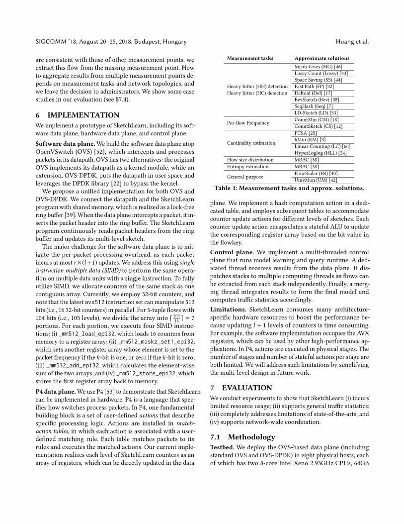
(Experiment 1) Memory usage. As per R1, Figure 6 showsthat 64KB memory suffices for SketchLearn (SL) to achieve

the desired errors. This is comparable and even much less

than many existing approaches. The only exception is that

cardinality estimation approaches require much less memory

as they do not need flow frequency and flowkey information,

yet they are only designed for cardinality estimation.

(Experiment 2) Per-packet processing. As per R2, Fig-ure 7 shows the peak per-packet processing overhead in

CPU cycles. SketchLearn incurs only 92 cycles with SIMD,

much lower than the 200-cycle budget for 10Gbps links (a

67K 24K 21K 15K2.3K 4.7K 2.6K 2.6K

185 40753 55 154 153 126

1.2K 5.7K92

102

105

108

MGLossy

SS FP DelRev

SeqLD CM CS

PCSAKM LC HLL

MRACFR UM SL

CP

U C

ycle

s

Figure 7: (Exp#2) Peak per-packet overhead.

99.93 99.99 99.96

0

50

100

OVS OVSDPDK

Tofino

Thro

ughput

(Norm

aliz

ed %

)

Figure 8: (Exp#3)Testbed through-put.

26.71

15.55

0

10

20

30

r=1 r=2

Thro

ughput

(MP

PS

)

Figure 9: (Exp#4)Simulatorthroughput.

1

2

3

1 2 3 4 5Number of Threads

Tim

e (

s) 64K

128K

Figure 10: (Exp#5)Inference time.

non-SIMD version incurs 600 CPU cycles, not shown in the

figure). For comparisons, top-k approaches consume an order

of 104CPU cycles as they traverse the whole data structure

in the worst case. Some sketch-based approaches (e.g., CM)

also fulfill the requirements, but they are specialized. Other

sketch-based solutions (e.g., FR and UM) employ complicated

structures to be general-purpose but incur high overhead.

(Experiment 3) Testbed throughput. We measure the

throughput of SketchLearn in both OVS-based and P4 plat-

forms. Figure 8 shows the normalized throughput to the

line-rate speed without measurement. The processing speed

is preserved and the variance is very small. The high perfor-

mance comes from the fact that counters in different levels

have no dependencies, providing opportunities for paral-

lelization in both software and hardware platforms (see §6).

In particular, for P4, counter update actions are distributed

in different physical stages and executed in parallel.

(Experiment 4) Simulator throughput. Figure 9 presentsthe throughput of SketchLearn for r = 1 and r = 2 per level

in our stress-test simulator. The throughput is above the

14.88Mpps requirement for 64-byte packets in a 10Gbps link.

(Experiment 5) Inference time. As per R3, we measure

the model inference time (see §4.3). Figure 10 shows that the

model inference time decreases as the number of threads

grows. With five threads, the inference time takes less than

0.5 seconds. Doubling the sketch size only slightly increases

the inference time, as the large flow extraction converges

faster with more stacks and preserves the total time.

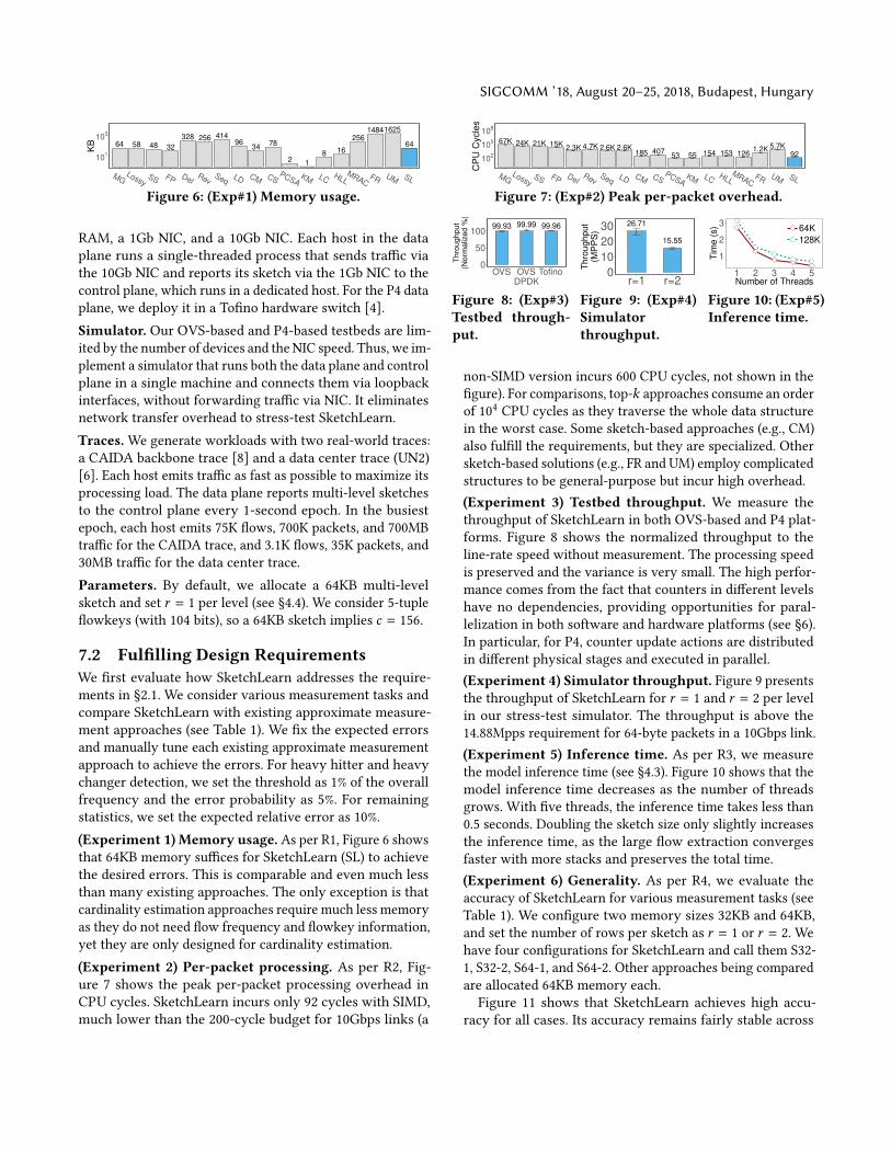
(Experiment 6) Generality. As per R4, we evaluate the

accuracy of SketchLearn for various measurement tasks (see

Table 1). We configure two memory sizes 32KB and 64KB,

and set the number of rows per sketch as r = 1 or r = 2. We

have four configurations for SketchLearn and call them S32-

1, S32-2, S64-1, and S64-2. Other approaches being compared

are allocated 64KB memory each.

Figure 11 shows that SketchLearn achieves high accu-

racy for all cases. Its accuracy remains fairly stable across

SIGCOMM ’18, August 20–25, 2018, Budapest, Hungary Huang et al.

10

0

91

.8

10

0

10

0

10

0

98

.4

10

0

10

0

50

.4

60

.3

57

12

.6

10

0

82

.7

10

0

98

.7

00

96

.7

3.1

93

.3

86

.4

98

.4

97

.5

10

0

10

0

10

0

10

0

0

50

100

MGLossy

SS FP DelRev

SeqLD FR UM

S32−1S32−2

S64−1S64−2

Accu

racy (

%)

PrecisionRecall

(a) Heavy hitter

98

.8

84

.4

99

.2

97

.3

98

.4

94

.5

99

.5

97

.9

47

.6

62

.3

73

.2

11

94

.7

85

.5

10

0

88

.1

00

84

.2

2.7

91

.8

81

.4

97

.7

92

.8

10

0

10

0

10

0

10

0

0

50

100

MGLossy

SS FP DelRev

SeqLD FR UM

S32−1S32−2

S64−1S64−2

Accu

racy (

%)

PrecisionRecall

(b) Heavy changer

0.6

1

1.2

1

100

47.0

1

11.6

7

7.9

2

7.0

7

4.4

6

0

20

40

60

80

100

CM CS FR UMS32−1

S32−2S64−1

S64−2

Re

lative

Err

or

(%)

1.7

3

3.1

4

4.2

6

0.8

1

100

49.2

3

3.0

7

2.6

4

2.9

2.2

30

20

40

60

80

100

PCSAKM LC HLL

FR UMS32−1

S32−2S64−1

S64−2

Re

lative

Err

or

(%)

(c) Flow frequency (d) Cardinality

0.3

45

0.3

483

0.2

134

0.2

244

0.2

197

0.2

135

0.0

0.2

0.4

0.6

MRACUM

S32−1S32−2

S64−1S64−2

MR

D (

%)

3.8

4

27.0

9

16.4

6

11.8

9

11.7

2

9.3

5

0

10

20

30

40

50

MRACUM

S32−1S32−2

S64−1S64−2

Re

lative

Err

or

(%)

(e) Flow size distribution (f) Entropy

Figure 11: (Exp#6) Generality.

all four configurations as it can extract very small flows

to produce accurate results. Although its error is higher

than the best state-of-the-art for some cases (e.g., HLL for

cardinality), those state-of-the-arts are specialized. In par-

ticular, SketchLearn outperforms the two general-purpose

approaches FlowRadar and UnivMon, as they need excessive

memory (see Figure 6) to mitigate errors. With only 64KB

of memory, they suffer from serious hash collisions. In par-

ticular, FlowRadar fails to extract flows as it requires that

some counters contain exactly one flow in order for the flow

to be extracted; UnivMon has significant overestimates (see

Figure 11(c)) and hence high false positives (see Figure 11(a)).

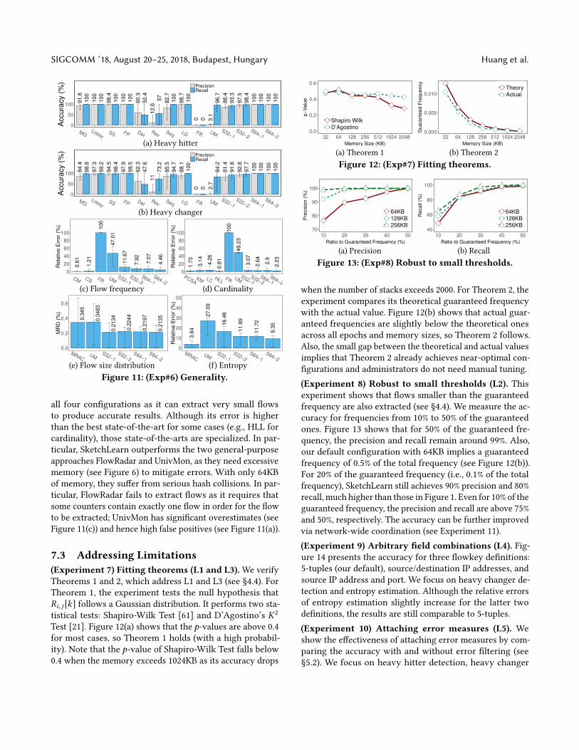
7.3 Addressing Limitations(Experiment 7) Fitting theorems (L1 and L3).We verify

Theorems 1 and 2, which address L1 and L3 (see §4.4). For

Theorem 1, the experiment tests the null hypothesis that

Ri, j [k] follows a Gaussian distribution. It performs two sta-

tistical tests: Shapiro-Wilk Test [61] and D’Agostino’s K2

Test [21]. Figure 12(a) shows that the p-values are above 0.4for most cases, so Theorem 1 holds (with a high probabil-

ity). Note that the p-value of Shapiro-Wilk Test falls below

0.4 when the memory exceeds 1024KB as its accuracy drops

0.0

0.2

0.4

0.6

32 64 128 256 512 1024 2048

Memory Size (KB)

p−

Valu

e

Shapiro Wilk

D’Agostino0.000

0.005

0.010

32 64 128 256 512 1024 2048

Memory Size (KB)

Guara

nte

ed F

requency

Theory

Actual

(a) Theorem 1 (b) Theorem 2

Figure 12: (Exp#7) Fitting theorems.

70

80

90

100

10 20 30 40 50

Ratio to Guaranteed Frequency (%)

Pre

cis

ion (

%)

64KB

128KB

256KB40

60

80

100

10 20 30 40 50

Ratio to Guaranteed Frequency (%)

Recall

(%)

64KB

128KB

256KB

(a) Precision (b) Recall

Figure 13: (Exp#8) Robust to small thresholds.

when the number of stacks exceeds 2000. For Theorem 2, the

experiment compares its theoretical guaranteed frequency

with the actual value. Figure 12(b) shows that actual guar-

anteed frequencies are slightly below the theoretical ones

across all epochs and memory sizes, so Theorem 2 follows.

Also, the small gap between the theoretical and actual values

implies that Theorem 2 already achieves near-optimal con-

figurations and administrators do not need manual tuning.

(Experiment 8) Robust to small thresholds (L2). Thisexperiment shows that flows smaller than the guaranteed

frequency are also extracted (see §4.4). We measure the ac-

curacy for frequencies from 10% to 50% of the guaranteed

ones. Figure 13 shows that for 50% of the guaranteed fre-

quency, the precision and recall remain around 99%. Also,

our default configuration with 64KB implies a guaranteed

frequency of 0.5% of the total frequency (see Figure 12(b)).

For 20% of the guaranteed frequency (i.e., 0.1% of the total

frequency), SketchLearn still achieves 90% precision and 80%

recall, much higher than those in Figure 1. Even for 10% of the

guaranteed frequency, the precision and recall are above 75%

and 50%, respectively. The accuracy can be further improved

via network-wide coordination (see Experiment 11).

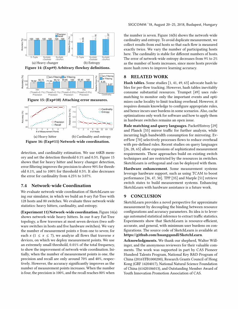
(Experiment 9) Arbitrary field combinations (L4). Fig-ure 14 presents the accuracy for three flowkey definitions:

5-tuples (our default), source/destination IP addresses, and

source IP address and port. We focus on heavy changer de-

tection and entropy estimation. Although the relative errors

of entropy estimation slightly increase for the latter two

definitions, the results are still comparable to 5-tuples.

(Experiment 10) Attaching error measures (L5). We

show the effectiveness of attaching error measures by com-

paring the accuracy with and without error filtering (see

§5.2). We focus on heavy hitter detection, heavy changer

SIGCOMM ’18, August 20–25, 2018, Budapest, Hungary

100100 100100 100100

0

50

100

5−Tuple SrcAddr+DstAddr

SrcAddr+SrcPort

Accu

racy (

%)

PrecisionRecall

9.3

5

11.1

6

11.9

7

0

5

10

15

5−Tuple SrcAddr+DstAddr

SrcAddr+SrcPort

Re

lative

Err

or

(%)

(a) Heavy changer (b) Entropy

Figure 14: (Exp#9) Arbitrary flowkey definitions.

92.7278.92

94.1271.34

10094.85 10095.45

0

50

100

HH(Thresh=0.1%)

Precision

HC(Thresh=0.1%)

Precision

HH(Thresh=0.5%)

Precision

HC(Thresh=0.5%)

Precision

Accura

cy (

%)

w/o Filtering w/ Filtering

3.074.25

0

5

CardinalityR

ela

tive

Err

or

(%) w/o Filtering

w/ Filtering

Figure 15: (Exp#10) Attaching error measures.

40

60

80

100

1 2 3 4 5 6 7# of Measurement Points

Accura

cy (

%)

Precision

Recall0.0

2.5

5.0

7.5

10.0

1 2 4 8 16 32 64 128# of Hosts

Rela

tive

Err

or

(%) Cardinality

Entropy

(a) Heavy hitter (b) Cardinality and entropy

Figure 16: (Exp#11) Network-wide coordination.

detection, and cardinality estimation. We use 64KB mem-

ory and set the detection threshold 0.1% and 0.5%. Figure 15

shows that for heavy hitter and heavy changer detection,

error filtering improves the precision to above 90% for thresh-

old 0.1%, and to 100% for threshold 0.5%. It also decreases

the error for cardinality from 4.25% to 3.07%.

7.4 Network-wide CoordinationWe evaluate network-wide coordination of SketchLearn us-

ing our simulator, in which we build an 8-ary Fat-Tree with

128 hosts and 80 switches. We evaluate three network-wide

statistics: heavy hitters, cardinality, and entropy.

(Experiment 11)Network-wide coordination. Figure 16(a)shows network-wide heavy hitters. In our 8-ary Fat-Tree

topology, a flow traverses at most seven devices (two soft-

ware switches in hosts and five hardware switches). We vary

the number of measurement points x from one to seven; for

each x (1 ≤ x ≤ 7), we analyze all flows that traverse xdevices, on which we deploy measurement points. We use

an extremely small threshold, 0.01% of the total frequency,

to show the improvement of network-wide coordination. Ini-

tially, when the number of measurement points is one, the

precision and recall are only around 70% and 40%, respec-

tively. However, the accuracy significantly improves as the

number of measurement points increases. When the number

is four, the precision is 100%, and the recall reaches 80% when

the number is seven. Figure 16(b) shows the network-wide

cardinality and entropy. To avoid duplicate measurement, we

collect results from end hosts so that each flow is measured

exactly twice. We vary the number of participating hosts

here. The cardinality is stable for different numbers of hosts.

The error of network-wide entropy decreases from 9% to 2%

as the number of hosts increases, since more hosts provide

more hash rows to improve learning accuracy.

8 RELATED WORKHash tables. Some studies [1, 41, 49, 63] advocate hash ta-

bles for per-flow tracking. However, hash tables inevitably

consume substantial resources. Trumpet [49] uses rule-

matching to monitor only the important events and opti-

mizes cache locality to limit tracking overhead. However, it

requires domain knowledge to configure appropriate rules,

and hence incurs user burdens in some scenarios. Also, cache

optimizations only work for software and how to apply them

in hardware switches remains an open issue.

Rule matching and query languages. PacketHistroy [29]and Planck [55] mirror traffic for further analysis, while

incurring high bandwidth consumption for mirroring. Ev-

erFlow [70] selectively processes flows to reduce overhead

with pre-defined rules. Recent studies on query languages

[26, 28, 65] allow expressions of sophisticated measurement

requirements. These approaches build on existing switch

techniques and are restricted by the resources in switches.

SketchLearn is orthogonal and can be deployed with them.

Hardware enhancement. Some measurement systems

leverage hardware support, such as using TCAM to boost

performance [36, 47, 50]. TPP [35] and Marple [51] retrieve

switch states to build measurement systems. Enhancing

SketchLearn with hardware assistance is a future work.

9 CONCLUSIONSketchLearn provides a novel perspective for approximate

measurement by decoupling the binding between resource

configurations and accuracy parameters. Its idea is to lever-

age automated statistical inference to extract traffic statistics.

Experiments show that SketchLearn is resource-efficient,

accurate, and general, with minimum user burdens on con-

figurations. The source code of SketchLearn is available at:

https://github.com/huangqundl/SketchLearn.Acknowledgments.We thank our shepherd, Walter Will-

inger, and the anonymous reviewers for their valuable com-

ments. The work was supported in part by CAS Pioneer

Hundred Talents Program, National Key R&D Program of

China (2016YFB1000200), Research Grants Council of Hong

Kong (GRF 14204017), National Natural Science Foundation

of China (61420106013), and Outstanding Member Award of

Youth Innovation Promotion Association of CAS.

SIGCOMM ’18, August 20–25, 2018, Budapest, Hungary Huang et al.

REFERENCES[1] Omid Alipourfard, Masoud Moshref, and Minlan Yu. 2015. Re-

evaluating Measurement Algorithms in Software. In Proc. of HotNets.[2] Mohammad Alizadeh, Albert Greenberg, David A Maltz, and Jitendra

Padhye. 2010. Data Center TCP (DCTCP). In Proc. of SIGCOMM.

[3] Ziv Bar-Yossef, T. S. Jayram, Ravi Kumar, D. Sivakumar, and Luca

Trevisan. 2002. Counting Distinct Elements in a Data Stream. In Proc.of RANDOM.

[4] Barefoot’s Tofino. 2018. https://www.barefootnetworks.com/

technology. (2018).

[5] Ran Ben Basat, Gil Einziger, Roy Friedman, Marcelo C Luizelli, and

Erez Waisbard. 2017. Constant Time Updates in Hierarchical Heavy

Hitters. In Proc. of SIGCOMM.

[6] Theophilus Benson, Aditya Akella, and David A. Maltz. 2010. Network

Traffic Characteristics of Data Centers in the Wild. In Proc. of IMC.[7] Tian Bu, Jin Cao, Aiyou Chen, and Patrick P. C. Lee. 2010. Sequential

Hashing: A Flexible Approach for Unveiling Significant Patterns in

High Speed Networks. Computer Networks 54, 18 (2010), 3309–3326.[8] Caida Anonymized Internet Traces 2016 Dataset. 2018. http://www.

caida.org/data/passive/passive_2016_dataset.xml. (2018).

[9] Marco Canini, Damien Fay, David J. Miller, AndrewW. Moore, and Raf-

faele Bolla. 2009. Per Flow Packet Sampling for High-Speed Network

Monitoring. In Proc. of COMSNETS.[10] George Casella and Roger Berger. 2001. Statistical Inference. Duxbury

Resource Center.

[11] Amit Chakrabarti, Graham Cormode, and Andrew Mcgregor. 2007. A

Near-Optimal Algorithm for Computing the Entropy of a Stream. In

Proc. of SODA.[12] Moses Charikar, Kevin Chen, and Martin Farach-Colton. 2004. Finding

Frequent Items in Data Streams. Theoretical Computer Science 312, 1(2004), 3–15.

[13] Surajit Chaudhuri, Bolin Ding, and Srikanth Kandula. 2017. Approxi-

mate Query Processing: No Silver Bullet. In Proc. of SIGMOD.[14] Yi-Chao Chen, Lili Qiu, Yin Zhang, Guangtao Xue, and Zhenxian Hu.

2014. Robust Network Compressive Sensing. In Proc. of MOBICOM.

[15] Graham Cormode and Marios Hadjieleftheriou. 2010. Methods for

Finding Frequent Items in Data Streams. The VLDB Journal 19, 1 (2010),3–20.

[16] Graham Cormode, Flip Korn, S. Muthukrishnan, and Divesh Srivastava.

2003. Finding Hierarchical Heavy Hitters in Data Streams. In Proc. ofVLDB.

[17] Graham Cormode and S. Muthukrishnan. 2004. What’s New: Finding

Significant Differences in Network Data Streams. In Proc. of IEEEINFOCOM.

[18] Graham Cormode and S. Muthukrishnan. 2005. An Improved Data

Stream Summary: The Count-Min Sketch and its Applications. Journalof Algorithms 55, 1 (2005), 58–75.

[19] Graham Cormode and S. Muthukrishnan. 2005. Space Efficient Mining

of Multigraph Streams. In Proc. of PODS.[20] Ítalo Cunha, Renata Teixeira, Nick Feamster, and Christophe Diot. 2009.

Measurement Methods for Fast and Accurate Blackhole Identification

with Binary Tomography. In Proc. of IMC.[21] Ralph D’Agostino and Egon S Pearson. 1973. Tests for Departure

from Normality. Empirical Results for the Distributions of b2and

√b1.

Biometrika 60, 3 (1973), 613–622.[22] Data Plane Development Kit. 2018. https://dpdk.org. (2018).

[23] Xenofontas Dimitropoulos, Paul Hurley, and Andreas Kind. 2008. Prob-

abilistic Lossy Counting: An Efficient Algorithm for Finding Heavy

Hitters. ACM SIGCOMMComputer Communication Review 38, 1 (2008).

[24] Philippe Flajolet, Éric Fusy, Olivier Gandouet, and Frédéric Meunier.

2007. HyperLogLog: The Analysis of A Near-optimal Cardinality

Estimation Algorithm. In Proc. of AOFA. 127–146.[25] Philippe Flajolet and G. Nigel Martin. 1985. Probabilistic Counting

Algorithms for Data Base Applications. J. Comput. System Sci. 31, 2(1985), 182–209.

[26] Nate Foster, RobHarrison,Michael J. Freedman, ChristopherMonsanto,

Jennifer Rexford, Alec Story, and David Walker. 2011. Frenetic: A

Network Programming Language. In Proc. of ICFP.[27] Sriram Govindan, Jie Liu, Aman Kansal, and Anand Sivasubramaniam.

2011. Cuanta: Quantifying Effects of Shared On-chip Resource Inter-

ference for Consolidated Virtual Machines. In Proc. of SoCC.[28] Arpit Gupta, Rüdiger Birkner, Marco Canini, Nick Feamster, Chris

Mac-Stoker, and Walter Willinger. 2016. Network Monitoring as a

Streaming Analytics Problem. In Proc. of HotNets.[29] Nikhil Handigol, Brandon Heller, Vimalkumar Jeyakumar, David Maz-

ières, and Nick McKeown. 2014. I Know What Your Packet Did Last

Hop: Using Packet Histories to Troubleshoot Networks. In Proc. ofNSDI.

[30] Nicholas J.A. Harvey, Jelani Nelson, and Krzysztof Onak. 2008. Sketch-

ing and Streaming Entropy via Approximation Theory. In Proc. ofFOCS.

[31] StefanHeule,Marc Nunkesser, andAlexanderHall. 2013. HyperLogLog

in Practice: Algorithmic Engineering of a State of The Art Cardinality

Estimation Algorithm. In Proc. of EDBT.[32] QunHuang, Xin Jin, Patrick P C Lee, Runhui Li, Lu Tang, Yi-Chao Chen,

and Gong Zhang. 2017. SketchVisor: Robust Network Measurement

for Soţtware Packet Processing. In Proc. of SIGCOMM.

[33] Qun Huang and Patrick P. C. Lee. 2015. A Hybrid Local and Distributed

Sketching Design for Accurate and Scalable Heavy Key Detection in

Network Data Streams. Computer Networks 91 (2015), 298–315.[34] Qun Huang, Patrick P. C. Lee, and Yungang Bao. 2018.

SketchLearn: Relieving User Burdens in Approximate Mea-

surement with Automated Statistical Inference (Technical Report).

https://github.com/huangqundl/SketchLearn/blob/master/TechReport.pdf.

(2018).

[35] Vimalkumar Jeyakumar, Mohammad Alizadeh, Yilong Geng,

Changhoon Kim, and David Mazières. 2014. Millions of Little Minions:

Using Packets for Low Latency Network Programming and Visibility.

In Proc. of SIGCOMM.

[36] Lavanya Jose, Minlan Yu, and Jennifer Rexford. 2011. Online Measure-

ment of Large Traffic Aggregates on Commodity Switches. In USENIXHotICE.

[37] Srikanth Kandula and Ratul Mahajan. 2009. Sampling Biases in Net-

work Path Measurements andWhat To Do About It. In Proc. of IMC.[38] Abhishek Kumar, Minho Sung, Jun (Jim) Xu, and Jia Wang. 2004. Data

Streaming Algorithms for Efficient and Accurate Estimation of Flow

Size Distribution. In Proc. of SIGMETRICS.[39] Patrick P. C. Lee, Tian Bu, and Girish Chandranmenon. 2010. A Lock-

Free, Cache-Efficient Multi-Core Synchronization Mechanism for Line-

Rate Network Traffic Monitoring. In Proc. of IPDPS.[40] Yuliang Li, RuiMiao, Changhoon Kim, andMinlan Yu. 2016. FlowRadar:

A Better NetFlow for Data Centers. In Proc. of NSDI.[41] Xuemei Liu, Meral Shirazipour, Minlan Yu, and Ying Zhang. 2016.

MOZART: Temporal Coordination of Measurement. In Proc. of SOSR.[42] Zaoxing Liu, Antonis Manousis, Gregory Vorsanger, Vyas Sekar, and

Vladimir Braverman. 2016. One Sketch to Rule Them All: Rethinking

Network Flow Monitoring with UnivMon. In Proc. of SIGCOMM.

[43] Gurmeet Singh Manku. 2002. Approximate Frequency Counts over

Data Streams. In Proc. of VLDB.[44] Ahmed Metwally, Divyakant Agrawal, and Amr El Abbadi. 2005. Effi-

cient Computation of Frequent and Top-k Elements in Data Streams.

In Proc. of ICDT.

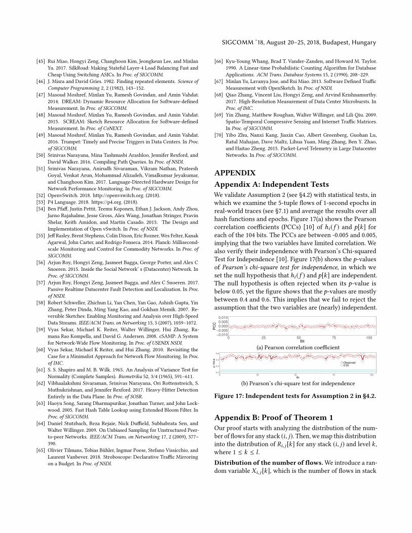
SIGCOMM ’18, August 20–25, 2018, Budapest, Hungary

[45] Rui Miao, Hongyi Zeng, Changhoon Kim, Jeongkeun Lee, and Minlan

Yu. 2017. SilkRoad: Making Stateful Layer-4 Load Balancing Fast and

Cheap Using Switching ASICs. In Proc. of SIGCOMM.

[46] J. Misra and David Gries. 1982. Finding repeated elements. Science ofComputer Programming 2, 2 (1982), 143–152.

[47] Masoud Moshref, Minlan Yu, Ramesh Govindan, and Amin Vahdat.

2014. DREAM: Dynamic Resource Allocation for Software-defined

Measurement. In Proc. of SIGCOMM.

[48] Masoud Moshref, Minlan Yu, Ramesh Govindan, and Amin Vahdat.

2015. SCREAM: Sketch Resource Allocation for Software-defined

Measurement. In Proc. of CoNEXT.[49] Masoud Moshref, Minlan Yu, Ramesh Govindan, and Amin Vahdat.

2016. Trumpet: Timely and Precise Triggers in Data Centers. In Proc.of SIGCOMM.

[50] Srinivas Narayana, Mina Tashmasbi Arashloo, Jennifer Rexford, and

David Walker. 2016. Compiling Path Queries. In Proc. of NSDI.[51] Srinivas Narayana, Anirudh Sivaraman, Vikram Nathan, Prateesh

Goyal, Venkat Arun, Mohammad Alizadeh, Vimalkumar Jeyakumar,

and Changhoon Kim. 2017. Language-Directed Hardware Design for

Network Performance Monitoring. In Proc. of SIGCOMM.

[52] OpenvSwitch. 2018. http://openvswitch.org. (2018).

[53] P4 Language. 2018. https://p4.org. (2018).

[54] Ben Pfaff, Justin Pettit, Teemu Koponen, Ethan J. Jackson, Andy Zhou,

Jarno Rajahalme, Jesse Gross, Alex Wang, Jonathan Stringer, Pravin

Shelar, Keith Amidon, and Martín Casado. 2015. The Design and

Implementation of Open vSwitch. In Proc. of NSDI.[55] Jeff Rasley, Brent Stephens, Colin Dixon, Eric Rozner,Wes Felter, Kanak

Agarwal, John Carter, and Rodrigo Fonseca. 2014. Planck: Millisecond-

scale Monitoring and Control for Commodity Networks. In Proc. ofSIGCOMM.

[56] Arjun Roy, Hongyi Zeng, Jasmeet Bagga, George Porter, and Alex C

Snoeren. 2015. Inside the Social Network’ s (Datacenter) Network. In

Proc. of SIGCOMM.

[57] Arjun Roy, Hongyi Zeng, Jasmeet Bagga, and Alex C Snoeren. 2017.

Passive Realtime Datacenter Fault Detection and Localization. In Proc.of NSDI.

[58] Robert Schweller, Zhichun Li, Yan Chen, Yan Gao, Ashish Gupta, Yin

Zhang, Peter Dinda, Ming Yang Kao, and Gokhan Memik. 2007. Re-

versible Sketches: Enabling Monitoring and Analysis over High-Speed

Data Streams. IEEE/ACM Trans. on Networking 15, 5 (2007), 1059–1072.[59] Vyas Sekar, Michael K. Reiter, Walter Willinger, Hui Zhang, Ra-

mana Rao Kompella, and David G. Andersen. 2008. cSAMP: A System

for Network-Wide Flow Monitoring. In Proc. of USENIX NSDI.[60] Vyas Sekar, Michael K Reiter, and Hui Zhang. 2010. Revisiting the

Case for a Minimalist Approach for Network Flow Monitoring. In Proc.of IMC.

[61] S. S. Shapiro and M. B. Wilk. 1965. An Analysis of Variance Test for

Normality (Complete Samples). Biometrika 52, 3/4 (1965), 591–611.[62] Vibhaalakshmi Sivaraman, Srinivas Narayana, Ori Rottenstreich, S.

Muthukrishnan, and Jennifer Rexford. 2017. Heavy-Hitter Detection

Entirely in the Data Plane. In Proc. of SOSR.[63] Haoyu Song, Sarang Dharmapurikar, Jonathan Turner, and John Lock-

wood. 2005. Fast Hash Table Lookup using Extended Bloom Filter. In

Proc. of SIGCOMM.

[64] Daniel Stutzbach, Reza Rejaie, Nick Duffield, Subhabrata Sen, and

Walter Willinger. 2009. On Unbiased Sampling for Unstructured Peer-

to-peer Networks. IEEE/ACM Trans. on Networking 17, 2 (2009), 377–

390.

[65] Olivier Tilmans, Tobias Bühler, Ingmar Poese, Stefano Vissicchio, and

Laurent Vanbever. 2018. Stroboscope: Declarative Traffic Mirroring

on a Budget. In Proc. of NSDI.

[66] Kyu-Young Whang, Brad T. Vander-Zanden, and Howard M. Taylor.

1990. A Linear-time Probabilistic Counting Algorithm for Database

Applications. ACM Trans. Database Systems 15, 2 (1990), 208–229.[67] Minlan Yu, Lavanya Jose, and Rui Miao. 2013. Software Defined Traffic

Measurement with OpenSketch. In Proc. of NSDI.[68] Qiao Zhang, Vincent Liu, Hongyi Zeng, and Arvind Krishnamurthy.

2017. High-Resolution Measurement of Data Center Microbursts. In

Proc. of IMC.[69] Yin Zhang, Matthew Roughan, Walter Willinger, and Lili Qiu. 2009.

Spatio-Temporal Compressive Sensing and Internet Traffic Matrices.

In Proc. of SIGCOMM.

[70] Yibo Zhu, Nanxi Kang, Jiaxin Cao, Albert Greenberg, Guohan Lu,

Ratul Mahajan, Dave Maltz, Lihua Yuan, Ming Zhang, Ben Y. Zhao,

and Haitao Zheng. 2015. Packet-Level Telemetry in Large Datacenter

Networks. In Proc. of SIGCOMM.

APPENDIXAppendix A: Independent TestsWe validate Assumption 2 (see §4.2) with statistical tests, in

which we examine the 5-tuple flows of 1-second epochs in

real-world traces (see §7.1) and average the results over all

hash functions and epochs. Figure 17(a) shows the Pearson

correlation coefficients (PCCs) [10] of hi (f ) and p[k] foreach of the 104 bits. The PCCs are between -0.005 and 0.005,

implying that the two variables have limited correlation. We

also verify their independence with Pearson’s Chi-squared

Test for Independence [10]. Figure 17(b) shows the p-valuesof Pearson’s chi-square test for independence, in which we

set the null hypothesis that hi (f ) and p[k] are independent.The null hypothesis is often rejected when its p-value is

below 0.05, yet the figure shows that the p-values are mostly

between 0.4 and 0.6. This implies that we fail to reject the

assumption that the two variables are (nearly) independent.

−0.010

−0.005

0.000

0.005

0.010

0 25 50 75 100Bit

PC

C

(a) Pearson correlation coefficient

0.0

0.2

0.4

0.6

0 25 50 75 100

Bit

p−

Va

lue

Observed0.05

(b) Pearson’s chi-square test for independence

Figure 17: Independent tests for Assumption 2 in §4.2.

Appendix B: Proof of Theorem 1Our proof starts with analyzing the distribution of the num-

ber of flows for any stack (i, j). Then, wemap this distribution

into the distribution of Ri, j [k] for any stack (i, j) and level k ,where 1 ≤ k ≤ l .

Distribution of the number of flows.We introduce a ran-

dom variable Xi, j [k], which is the number of flows in stack

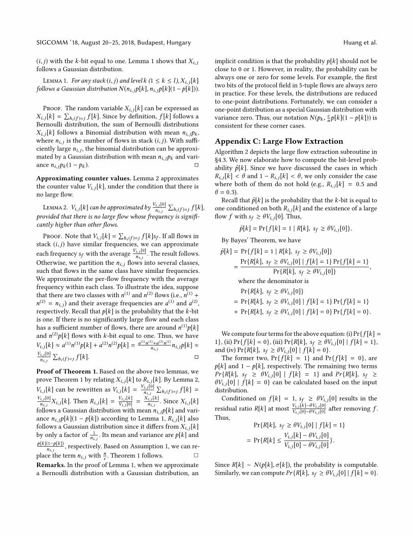
SIGCOMM ’18, August 20–25, 2018, Budapest, Hungary Huang et al.

(i, j) with the k-bit equal to one. Lemma 1 shows that Xi, jfollows a Gaussian distribution.

Lemma 1. For any stack (i, j) and levelk (1 ≤ k ≤ l),Xi, j [k]follows a Gaussian distribution N (ni, jp[k],ni, jp[k](1−p[k])).

Proof. The random variable Xi, j [k] can be expressed as

Xi, j [k] =∑hi (f )=j f [k]. Since by definition, f [k] follows a

Bernoulli distribution, the sum of Bernoulli distributions

Xi, j [k] follows a Binomial distribution with mean ni, jpk ,where ni, j is the number of flows in stack (i, j). With suffi-

ciently large ni, j , the binomial distribution can be approxi-

mated by a Gaussian distribution with mean ni, jpk and vari-

ance ni, jpk (1 − pk ). �

Approximating counter values. Lemma 2 approximates

the counter value Vi, j [k], under the condition that there is

no large flow.

Lemma 2. Vi, j [k] can be approximated by Vi, j [0]ni, j

∑hi (f )=j f [k],

provided that there is no large flow whose frequency is signifi-cantly higher than other flows.

Proof. Note that Vi, j [k] =∑hi (f )=j f [k]sf . If all flows in

stack (i, j) have similar frequencies, we can approximate

each frequency sf with the averageVi, j [0]ni, j

. The result follows.

Otherwise, we partition the ni, j flows into several classes,

such that flows in the same class have similar frequencies.

We approximate the per-flow frequency with the average

frequency within each class. To illustrate the idea, suppose

that there are two classes with n(1) and n(2) flows (i.e., n(1) +n(2) = ni, j ) and their average frequencies are a(1) and a(2),respectively. Recall that p[k] is the probability that the k-bitis one. If there is no significantly large flow and each class

has a sufficient number of flows, there are around n(1)p[k]and n(2)p[k] flows with k-bit equal to one. Thus, we have

Vi, j [k] ≈ a(1)n(1)p[k] + a(2)n(2)p[k] = a(1)n(1)+a(2)n(2)

ni, jni, jp[k] ≈

Vi, j [0]ni, j

∑hi (f )=j f [k]. �

Proof of Theorem 1. Based on the above two lemmas, we

prove Theorem 1 by relating Xi, j [k] to Ri, j [k]. By Lemma 2,

Vi, j [k] can be rewritten as Vi, j [k] =Vi, j [0]ni, j

∑hi (f )=j f [k] =

Vi, j [0]ni, j

Xi, j [k]. Then Ri, j [k] =Vi, j [k ]Vi, j [0]

=Xi, j [k ]ni, j

. Since Xi, j [k]

follows a Gaussian distribution with mean ni, jp[k] and vari-

ance ni, jp[k](1 − p[k]) according to Lemma 1, Ri, j [k] alsofollows a Gaussian distribution since it differs from Xi, j [k]by only a factor of

1

ni, j. Its mean and variance are p[k] and

p[k ](1−p[k])ni, j

, respectively. Based on Assumption 1, we can re-

place the term ni, j withnc . Theorem 1 follows. ✷

Remarks. In the proof of Lemma 1, when we approximate

a Bernoulli distribution with a Gaussian distribution, an

implicit condition is that the probability p[k] should not be

close to 0 or 1. However, in reality, the probability can be

always one or zero for some levels. For example, the first

two bits of the protocol field in 5-tuple flows are always zero

in practice. For these levels, the distributions are reduced

to one-point distributions. Fortunately, we can consider a

one-point distribution as a special Gaussian distribution with

variance zero. Thus, our notation N (pk ,cnp[k](1 − p[k])) is

consistent for these corner cases.

Appendix C: Large Flow ExtractionAlgorithm 2 depicts the large flow extraction subroutine in

§4.3. We now elaborate how to compute the bit-level prob-

ability p̂[k]. Since we have discussed the cases in which

Ri, j [k] < θ and 1 − Ri, j [k] < θ , we only consider the case

where both of them do not hold (e.g., Ri, j [k] = 0.5 and

θ = 0.3).Recall that p̂[k] is the probability that the k-bit is equal to

one conditioned on both Ri, j [k] and the existence of a large

flow f with sf ≥ θVi, j [0]. Thus,

p̂[k] = Pr{ f [k] = 1 | R[k], sf ≥ θVi, j [0]}.

By Bayes’ Theorem, we have

p̂[k] = Pr{ f [k] = 1 | R[k], sf ≥ θVi, j [0]}

=Pr{R[k], sf ≥ θVi, j [0] | f [k] = 1} Pr{ f [k] = 1}

Pr{R[k], sf ≥ θVi, j [0]},

where the denominator is

Pr{R[k], sf ≥ θVi, j [0]}

= Pr{R[k], sf ≥ θVi, j [0] | f [k] = 1} Pr{ f [k] = 1}

+ Pr{R[k], sf ≥ θVi, j [0] | f [k] = 0} Pr{ f [k] = 0}.

We compute four terms for the above equation: (i) Pr{ f [k] =1}, (ii) Pr{ f [k] = 0}, (iii) Pr{R[k], sf ≥ θVi, j [0] | f [k] = 1},

and (iv) Pr{R[k], sf ≥ θVi, j [0] | f [k] = 0}.

The former two, Pr{ f [k] = 1} and Pr{ f [k] = 0}, are

p[k] and 1 − p[k], respectively. The remaining two terms

Pr {R[k], sf ≥ θVi, j [0] | f [k] = 1} and Pr {R[k], sf ≥

θVi, j [0] | f [k] = 0} can be calculated based on the input

distribution.

Conditioned on f [k] = 1, sf ≥ θVi, j [0] results in the

residual ratio R[k] at mostVi, j [k ]−θVi, j [0]Vi, j [0]−θVi, j [0]

after removing f .

Thus,

Pr{R[k], sf ≥ θVi, j [0] | f [k] = 1}

= Pr{R[k] ≤Vi, j [k] − θVi, j [0]

Vi, j [0] − θVi, j [0]}.

Since R[k] ∼ N (p[k],σ [k]), the probability is computable.

Similarly, we can compute Pr {R[k], sf ≥ θVi, j [0] | f [k] = 0}.

SIGCOMM ’18, August 20–25, 2018, Budapest, Hungary

Algorithm 2 Large flow extraction subroutine

Input : threshold θ , stack (i, j), sketch S , bit-level counter distributions{N (p[k ], σ 2[k ])}

1: procedure ExtractLargeFlows

/* Estimate bit-level probabilities */2: for 1 ≤ k ≤ l do3: Compute p̂[k ]

/* Find candidate flowkeys */4: Set the set of candidate flows C = ∅

5: Set template T as an empty string

6: for 1 ≤ k ≤ l do7: if p̂[k ] > 0.99 then8: Append ‘1’ to T9: else if 1 − p̂[k ] > 0.99 then10: Append ‘0’ to T11: else12: Append ‘*’ to T13: for all f matching T do14: if hi (f ) == j then15: C = C ∪ {f }

/* Estimate frequencies */16: for all f ∈ C do17: for 1 ≤ k ≤ l do18: if f [k ] == 1 then19: Frequency estimate E[k ] =

Ri, j [k ]−p[k ][0]1−pk

Vi, j [0]20: else21: Frequency estimate E[k ] = (1 −

Ri, j [k ]p[k ] )Vi, j [0]

22: sf =Median({E[k ]})

/* Associate bit-level probabilities */23: for all f ∈ C do24: for 1 ≤ k ≤ l do25: if f [k ] == 1 then26: Associate probability p̂[k ] to the k-bit27: else28: Associate probability 1 − p̂[k ] to the k-bit

/* Verify candidate flowkeys */29: for all f ∈ C do30: for 1 ≤ i′ ≤ r, i′ , i do31: j′ = hi′ (f )32: for 1 ≤ k ≤ l do33: if f [k ] == 0 and Vi′, j′ [0] −Vi′, j′ [k ] < sf then34: sf = Vi′, j′ [0] −Vi′, j′ [k ]35: else if f [k ] == 1 and Vi′, j′ [k ] < sf then36: sf = Vi′, j′ [k ]

37: if sf < θ ×Vi, j [0] then38: Remove f from C39: return C

Appendix D: Proof of Theorem 2We now present the proof of Theorem 2. Note that Theorem 2

may fail in some extreme cases. One scenario is that all

large flows have a frequency exactly1

c of the total frequency,

and they are all unfortunately hashed to one single column.

However, we prove that such extreme cases happen with a

negligible probability. Thus, Theorem 2 holds in practice. We

start with one stack as Lemma 3.

Lemma 3. For stack (i, j) and flow f hashed to it, if sf >1

2Vi, j [0], f must be extracted.

The correctness of this lemma has been justified in §4.3.

Proof of Theorem 2. Recall that a hash function uniformly

hashes the remaining small flows to the c columns, and

each column receives less than1

c of the total frequency con-

tributed by the small flows.

If a stack has only one large flow, this large flow must

be extracted by Lemma 3 as its contribution is larger than

1

2. For a stack with multiple large flows, we start with the

case with two large flows and generalize it later. For the

two large flows, if one has twice frequency as the other, its

frequency must be larger than the sum of the smaller one and

the remaining small flows. Thus, it contributes more than1

2

of frequency and must be extracted. After its extraction, the

other large flow has a contribution above1

2and will also be

extracted.

Otherwise, their difference is small. In the worst case, the

two large flows have exactly1

c of the total frequency. Taking

the small flows into account, either large flow contributes1

3

of the stack frequency. Recall that the large flow extraction is

repeatedly invoked with varying parameter θ . When θ < 1

3,

the subroutine assigns a wildcard symbol * if the ratio in one

bit is not significant enough, and then enumerates all possible

flowkeys. Thus, the two large flows must be extracted as

long as the subroutine is invoked with θ < 1

3. The only

probability to miss them is that the algorithm terminates

before θ decreases below1

3.

In general, for a stack with t large flows, they are missed

only if: (i) all of the t large flows have similar frequencies

so that they cannot be extracted one by one; and (ii) all

stacks (including (i, j)) fit Gaussian distributions well before

θ decreases to1

t+1 .

However, this is almost impossible for three reasons. First

and the most importantly, the termination requires 99.73%

observed Ri, j [k] deviate p[k] within three standard devia-

tions. Given that a practical sketch in SketchLearn has only

hundreds of columns, the ratio 99.73% already includes all

stacks. Since a stack with multiple large flows usually far

deviates p[k], the algorithm will not terminate before ex-

tracting them. Second, network traffic is typically skewed,

particularly large flows have very diverse frequencies. Fi-

nally, the previous study [7] proves that the number of large

flows in a column follows a Poisson distribution. The proba-

bility of hashing quite a few large flows into one column is

very small. In summary, we conclude that the extreme cases

that fail Theorem 2 have a negligible probability and can be

ignored. ✷