- i

ASHRAE Journal

AIVC #13,513

Sizing and Balancing Air Duct Systems By Robert W. Besant, P.Eng., and Yaw Asiedu, Ph.D.

Fellow ASHRAE

0 f the three duct design procedures recommended by the 1997 ASHRAE Handbook-Fundamentals, o nly the

T-method incorporates life-cycle cost. This method requires many

computations, which makes non-cost optimizing techniques more attractive

to designers. A new least life-cycle cost, three-stage

procedure for air duct system design is discussed in this article. The Initial

Duct Sizing, Pressure Augmentation and Size Augmentation (IPS) method

has the potential to reduce ducting system life-cycle costs and the time it takes

to design them.

Ducting system design has many con­straints such as low acoustic noise lev­els, minimal heat gain or loss, no external water vapor condensation, insignificant leakage, good fire resistance, and good strength characteristics to resist implo­sion or duct deformation. These con­straints add to the cost per unit area of ducting.

However, the main function of ducting is to satisfy the airflow rates specified for each terminal for air diffusion in each air space or room and exhaust air from the same spaces. Thus, many air diffuser ter­minals will be supplied by conditioned air from the supply air fans while exhaust air will be gathered from many grilles for all rooms in the building.

Ducting systems are complex and ex­pensive. Studies show that HV AC air duct systems are one of the major electrical energy consumers in industrial and com­mercial buildings (Tsai et al. 1988a). The life-cycle operating costs for ducting air supply and exhaust systems often exceed the first cost (Carrier et al. 1998). A poor design of an air duct system will lead to wasted energy and/or excessive ductwork

material. Both of tbese increase the Life­Cycle Cost (LC ). Becallse newly installed ducting ystems 1,1sing t andard duct sizes usually don't satisfy the specified airfu>w rates for each room, they require a time-consuming balancing effo1t.

In designing an air duct system, the designer usually begins with a duct sys­tem layout and specified airflow rates. Th designer selects and speci:fie the materi­als for the ducts and fittings duct sizes and fan(s). Ideally these selections hould be made so that all the design

constraints are satisfied and the LCC is minimized. The LCC of a duct system com­prises the initial or first cost and the op­erating cost.

The initial cost includes the fan, mate­rials, labor, shop drawings, shipping and a mark up for overhead, maintenance and insurance. The operating cost is usually the energy cost and, for many existing designs, it will exceed the ducting system's first cost for life cycles of 10 to 20 years.

T_he cost directly attributable to a duct section in a system is given by the- sum of the operating and capital costs

(1) where the section pressure drop for a

steady flow rate Q is !'JP= ( fL + 2.., c) v2 P (2)

D" 2 and a life-cycle factor for operating

costs

z = (Ed+ EJ)PWEF 77/'7,,,

(3)

where E = Present worth owning and

Q operating cost (LCC)

= Airflow rate in duct section (m3/s)

L1 P = Pressure losses in duct section (Pa)

L D.,

f

= Unit duct cost as installed (cost/m2)

= Duct length (m) = Equivalent by cost diameter

(equal to D for circular and for rectangular ducts)(m)

= Friction factor D" = Hydraulic friction diameter (m) :LC = Summation of dynamic loss

coefficient for duct fittings within the duct section

= Flow velocity (mis) = Air density (m3/kg) = Energy demand cost (cost/kW) = Unit electrical energy cost

(cost/kWh)

About the Authors Robert W. Besant, P.Eng., is pro­fessor emeritus at the University of Saskatchew£1n, Canada. He is mem­ber of ASHRAE Technical Committee 5.5, Air-to-Air Energy Recovery. Yaw Asiedu, Ph.D., is -a research engineer at Venmar CES, Saskatoon, Saskatchewan.

24 ASHRAE Journal www.ash raejournal . org December 2000

ASHRAF;:Journal

T = Operational time (hours/year) PWEF = Present worth escalation

factor

1J 111 = Motor drive efficiency

77 / =Fan total efficiency.

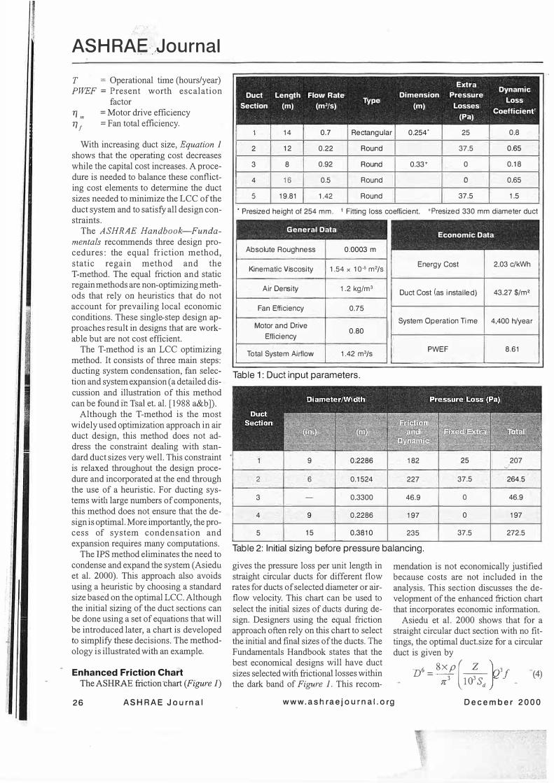
With increasing duct size, Equation 1 shows that the operating cost decreases while the capital cost increases. A proce­dure is needed to balance these conflict­ing cost elements to determine the duct sizes needed to minimize the LCC of the duct system and to satisfy all design con­straints.

The ASHRAE Handbook-Funda­mentals recommends three design pro­cedures: the equal friction method, static regain method and the T-method. The equal friction and static regain methods are non-optimizing meth­ods that rely on heuristics that do not account for prevailing local economic conditions. These single-step design ap­proaches result in designs that are work­able but are not cost efficient.

The T-method is an LCC optimizing method. It consists of three main steps: ducting system condensation, fan selec­tion and system expansion (a detailed dis­cussion and illustration of this method can be found ih Tsai et. al. [1988 a&b ]).

Although the T-method is the most widely used optimization approach in air duct design, this method does not ad­dress the constraint dealing with stan­dard duct sizes very well. This constraint is relaxed throughout the design proce­dure and incorporated at the end through the use of a heuristic. For ducting sys­tems with large numbers of components, this method does not ensure that the de­sign is optimal. More importantly, the pro­cess of system condensation and expansion requires many computations.

The IPS method eliminates the need to condense and expand the system (Asiedu et al. 2000). This approach also avoids using a heuristic by choosing a standard size based on the optimal LCC. Although the initial sizing of the duct sections can be done using a set of equations that will be introduced later, a chart is developed to simplify these decisions. The method­ology is illustrated with an example.

Enhanced Friction Chart The ASHRAE friction -chart (Figure 1)

26 ASH RAE J ournal

Extra . Dynamic

Duct Length Flow Rate Dimension Pressure L Type oss

Section (m) (m3/s) (m) Losses C ff" . tt

(Pa) oe 1c1en

14 0.7 Rectangular 0.254" 25 0:8

2 12 0.22 Round 37.5 0.65

3 8 0.92 Round 0.33+ 0 0.18

4 16 0.5 Round 0 0.65

5 19.81 1.42 Round 37.5 1.5

• Presized height of 254 mm. t Fitting loss coefficient. +Presized 330 mm diameter duct

General Data

Absolute Roughness 0.0003 m

Kinematic Viscosity 1 .54 x 1 0-5 m2/s

Air Density 1.2 kg/m3

Fan Efficiency 0.75

Motor and Drive 0.80

Efficiency

Total System Airflow 1.42 m3/s

Table 1 : Duct input parameters.

9 0:2286

2 6 0.1524

3 0.3300

4 9 0.2286

5 15 0.3810

Economic Data

Energy Cost 2.03 c/kWh

Duct Cost (as installed) 43.27 $/m2

System Operation T i me 4,400 h/year

182

227

46.9

197

235

PWEF 8.61

25 207

37.5 264.5

0 46.9

0 197

37.5 272.5

Table 2: Initial sizing before pressure balancing.

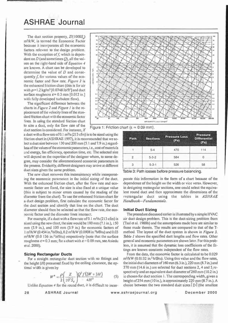
gives the pressure loss per unit length in straight circular ducts for different flow rates for ducts of selected diameter or air­flow velocity. This chart can be used to select the initial sizes of ducts during de­sign. Designers using the equal friction approach often rely on this chart to select the.initial and final sizes of the ducts. The Fundamentals Handbook states that the best economical designs will have duct sizes selected with frictional losses within the dark bana of Figure 1. This recom-

mendation is not economically justified because costs are not included in the analysis. This section discusses the de­velopment of the enhanced friction chart that incorporates economic information.

Asiedu et al. 2000 shows that for a straight circular duct section with no fit­tings, the optimal ducLsize for a circular duct is given by

D6 = 8xp(� h3J -(4) 77:3 103 sd r -

www.ash raej o urn al. o rg December 2000

ASHRAE Journal

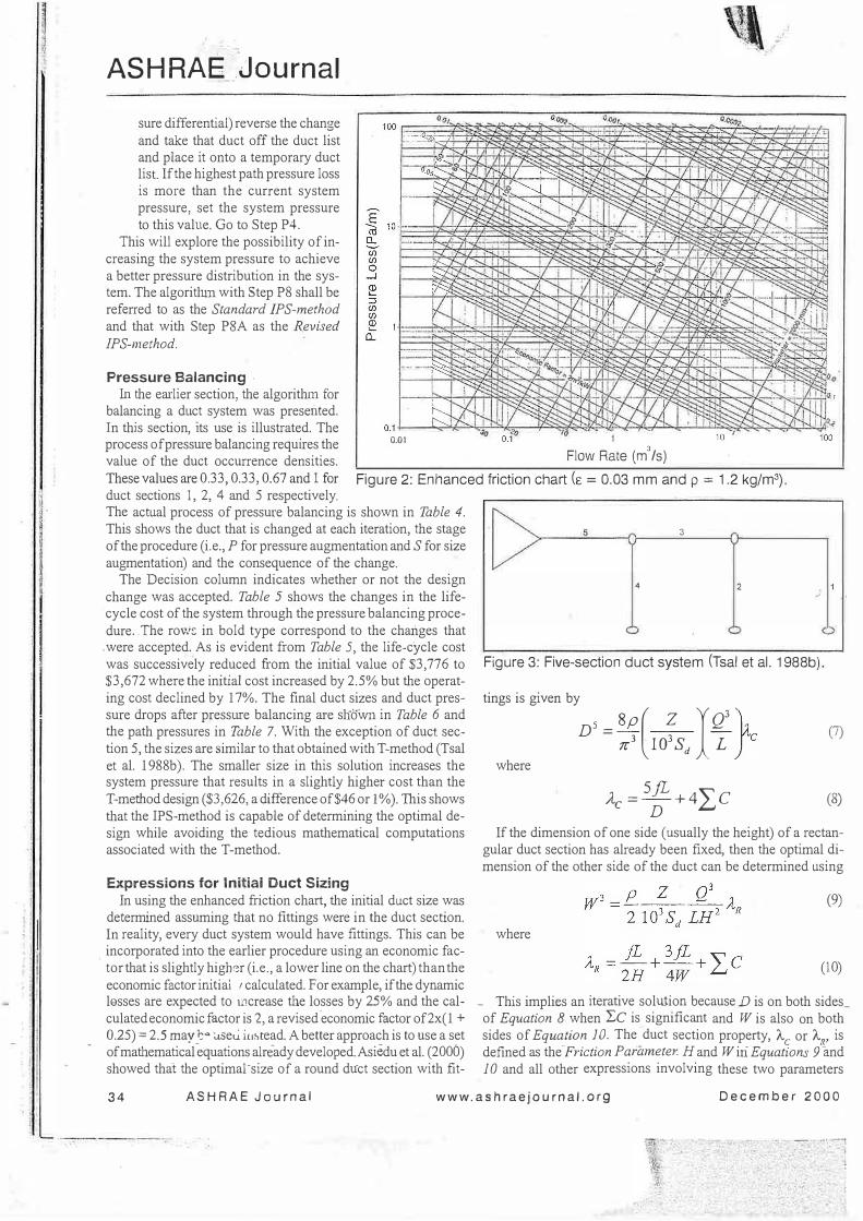
The duct section property, Z/( l 000,S:,) m2/k.W, is termed the Economic Factor because it incorporates all the economic factor relevant to the des ign problem. With the exception off, which is depen­dent on D (and sometimes Q), all the val­ues on the right-hand side of Equalio11 4 are known. A chart can be developed to determine the value of D and conse­quently f, for various values of the eco­nomic factor and flow rate. Figure 2 is the enhanced friction chart (this is for aiT with p = l .2 kglm3 (0.0748 lb/fPJ and duct sw·tace roughness e= 0.3 nun (0.012 in.) with fully developed turbulent flow).

The significant difference between the charts in Figure 2 and Figure 1 is the re­p.lacement of the velocity lines oftbe stan­dard ftiction chmt with the economi factor lines. In using the standard friction chart

0.3

0.2

�-�M�5BR��·;;::::;-:;µ::::=Fi ''° � 70 ',.../-..P.1.-,4.:::...;.J�,_:,/.....l--A-::.!..-J,4..,:� . ..i.1-__;:,.µ.._� l�+:'f.HI�...+.-�� .,.,,_.._.,.___, so ,""l-+JP..;.-,r--.:-f>'*+--1-11'>' L-M-�-i-J,� �/.f>o!.�....-�Px-l-1'--+"bl-l�i"""� �

Alll QUANTlTY, lls al 1.20 kglm3

to size a duct, only the flow rate of the Figure 1 : Friction chart (E = 0.09 mm). duct section is considered. For instance, if a duct with aflowrateof0.1 m3/s (213 cfm) is to be sized using the friction cl.tart in (ASHRAE 1997), it is reconm1e.nded that we se­lect a duel ize between 130 and 200 mm (5.1 and.7.9 in.) regard­les of tl1e val oes of the economic parameters i.e., cost of mate1ials cmd energy, fan efficiency, operation time, etc. The selected size will depend on the expertise of the de igner whom, to some de­gree, may consider the aforementioned economic parameters 'in the process. Evider1tly different designers may arrive at different duct izes give11 the same problem.

The new chart removes tl1(s incon istency while incorporat­ing the eco:nomic paramt::l1::!' in the initial sizing of the duct. With the enhanced friction chart, after the flow rate and eco­nomic facto�· are fixed, the size is also fixed al a un ique value (this is subject to minor errors caused by the reading of the d iameter from the chart). To use the enhanced friction chart for a duct design problem, first calculate the economic factor for the duct section and identify that line on the chart. The duct diameter should then be selected so that the flow rate, the eco­nomic factor and the diameter line intersect.

For example, ifa duct with allow rate ofO. I 013/s (213 cfm) is sized using the new chiut, the size would be 180 mm (7 .1 in.), 150 mm (5.9 in.), and 100 mm (3.9 in.) for economic factors of J m2/kW (0.454 in.2 h/Btu), 0.2 m2/kW (0.Q908 in .211/Btu) aod 0.03 m2/kW (0.0 136 in.2 h/Btu) respectively (note that the surface roughness e= 0.3 mm; for a chai:t with e == 0.09 mm ee Asiedu et al. 2000)�

Sizing Rectangular Ducts For a straight rectangular duct section with no fittings and

the height (ff) presumed fixed by the ceiling clearance, tbe op­timal width is given by

. w4 = P (_z _JQ3/(2W +3H) (5) 2 103Sd - 4Jfl Unlike Equation 4 for the rou11d duct, it is difficult to i11cor-

Pressure Loss Pressure

Path Sections Differential ' (Pa)

(Pa)

1 5.4 470 114

2 5-3-2 584 0

3 5-3-1 526 58

Table 3: Path losses before pressure balancing. porate tbi information in the form of a chru1 because of the dependence ofthe height ou lhe width or vice versll. However, in designing rectangular sections, one could select lhe equiva­lent round duct and tben approximate the dimensions of the rectangular duct using t h e tables in A.SHRAE Handbook-Fundamental .

Initial Duct Sizing The procedurecLiscusscd earlier is illustrnted by a simple HVAC

afr duct design problem. This is the duct-sizing problem from (Tsai et aJ. 198 b) and the assumptions made here are similar to those made therein. The results are compared to that of the T­method. The layout of the duct system is how.o in Figure 3. Table 1 shows the specified duct lengths and flow rates. Other general and economic parameters are hown later. For this prob­lem it is assumed that the dynamic loss coefficients of the fit­tings are known constants independent of the flow rates.

From the data the economic factor is calculated to be 0.029 m2/k.W (0.0132 in.2 h/Btu). Using this value and the flow rates, the initial duct diameters of 160 mm (6.3 in.), 220 mm (8.7 .in.) and 370 mm (14.6 in.) are selected for duct sections 2, 4 and 5_re­spectively and an equivalent duct diameter of260 mm (10.2 in.) i chosen· for duct section 1. The corresponcLing width, given a height of254 mm (I 0 in.), is approximateiy 220 mm (8.7 in.). A choice between the two standard duct sizes ID l (the smallest

28 ASHRAE Journal www.ashraejournal.org December 2000

J

s

------------·�----------------=------··��=-=�� ... ..:.__. ___ __, __

Table 4: Pressure balancing.

Iteration

1

2

3

4

5

Stage

p

p

s

p

s

Path Duct Selected Selected

1 4

3 1

2 2

1 4

3 1

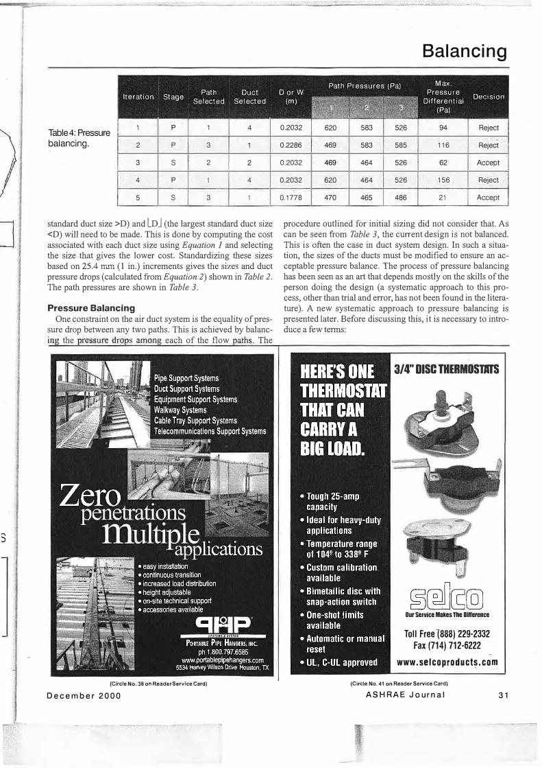
standard duct size >D) and LDJ (the largest standard duct size <D) will need to be made. This is done by computing the cost associated with each duct size using Equation 1 and selecting the size that gives the lower cost. Standardizing these sizes based on 25.4 mm (1 in.) increments gives the sizes and duct pressure drops (calculated from Equation 2) shown in Table 2. The path pressures are shown in Table 3.

Pressure Balancing One constraint on the air duct system is the equality of pres­

sure drop between any two paths. This is achieved by balanc­in • the ressure dro s amon each of the flow aths. The

(Circle No. 38 on Reader Service Card) December 2000

Balancing

Path Press ures (Pa) Max.

Dor W Pressure Oec1s1on (m) --- 01fferent1al

(Pa)

0.2032 620 583 526 94 Reject

0.2286 469 583 585 116 Reject

0:2032 469 464 526 62 Accept

0.2032 620 464 526 156 Reject

0.1778 470 465 486 21 Accept

procedure outlined for initial sizing did not consider that. As can be seen from Table 3, the current design is not balanced. This is often the case in duct system design. In such a situa­tion, the sizes of the ducts must be modified to ensure an ac­ceptable pressure balance. The process of pressure balancing has been seen as an art that depends mostly on the skills of the person doing the design (a systematic approach to this pro­cess, other than trial and error, has not been found in the litera­ture). A new systematic approach to pressure balancing is presented later. Before discussing this, it is necessary to intro­duce a few terms:

3/4" DISC THERMOSWS

Our Service Makes The Dlnerence

Toll Free 1888) 229-2332 Fax (714) 712-6222

www.selcoproduct�.com (Circle No. 41 on Reader Service Card)

ASHRAE Journal 31

ASHRAE Journal

Iteration Initial Cost ($) Energy Cost ($) Total Cost ($)

Initial 2,715 1,061 3,776

Design

1 2,660 1,128 3,788

2 2,685 1,064 3,749

3 2,757 957 3,714

4 2,702 1,128 3,830

5 2,783 884 3,672

Table 5: Tracking of LCC of duct system.

Dominant Path = the path with the highest path pressure loss. Dominant Section = a duct section on the dominant path. Path Pressure Differential = the difference between the domi­nant path pressure loss and the pressure loss of any other path.

Duct Occurrence Density is defined as

i5 = Number ofpaths with duct section x co11in101z (6) x Total number of paths

The aim of the new algorithm is to attempt to balance the system without increasing the initial system pressure. How­ever, when this is not possible, the algorithm permits an in­crease in the system pressure to balance the system. The algorithm given later is divided into two separate stages. These are the two latter stages of the three-stage duct sizing process, i.e., Initial Duct Sizing, Pressure Augmentation and Size Aug­mentation, henrn the mnemonic, !PS-Method. The two stages together constitute the pressure balancing procedure. Initial duct sizing using the Enhanced Friction Chart has already been discussed. As stated earlier, mathematical equations may be used for this purpose. They are presented in a later section.

Pressure Augmentation Pl. Identify the dominant path and sections. P2. Rank each path. Paths with higher path pressure differen­

tials must be ranked higher. Do not include the dominant path in this ranking.

P3. Rank the non-dominant duct sections according to the duct occurrence density Equation 6 in descending order. Do not include the ducts taken off the duct list in Step P6.

P4. Select the path at the top of the path list created in Step P2. If no path exists in the path list go to Step P9.

PS. Select the duct from the path that is ranked highest in the duct list created in Step P3. If no such duct section exists, take the path off the path list and go to Step P2.

P6. If the size can not be reduced any further, take the duct off the duct list and go to Step PS. Otherwise, reduce the size of this duct.

P7. Calculate the path pressures. P8. If the change in -Step P6 results in an unacceptable design

(i.e., violation of a constraint, a higher maximum pressure - differential or a change in the-dominant path without an

accompanying satisfactory path pressure distribution), re- -

10 0.2032 142 25 167

2 7 0.1524 108 37.5 145

3 0.3300 46.9 0 46.9

4 9 0.2032 197 0 197

5 15 0.3810 235 37.5 272

Table 6: Duct sizes and section pressure losses after pres-sure balancing.

Path Sections Pressure Loss Pressure

(Pa) Differential (Pa)

1 5-4 470 16

2 5-3-2 465 21

3 5-3-1 486 0

Table 7: Path losses after pressure balancing.

verse the change and take that duct off the duct list onto a temporary duct list and go to Step P4.

P9. If the pressure distribution is satisfactory, stop and select the fan. Otherwise, if there are no more paths on the path list and no ducts on the temporary duct lists, go to the Size Augmentation stage. Go to Step P2.

Size Augmentation Sl. Rank the dominant sections according to the duct occur­

rence density in ascending order. However, do not include any duct with o = 1.

S2. Select the duct ranked highest in the duct list created in Step 1. If no duct sections exist, stop. That is th� best possible design. Select the fan.

S3. If the size of the duct section cannot be further increased, take the duct off the duct list and go to Step S2. Otherwise, increase the size of this duct.

S4. Calculate all the new path pressures. SS. If the change in Step S3 results in a violation of a constraint

or a higher maximum pressure differential, reverse the change and take that duct off the duct list and go to Step S2.

S6. If the pressure distribution is satisfactory, stop and select the fan. Otherwise, go to Step Pl .

It i s conceivable that the algorithm's exit from Step S2 will result in a final design that will have a maximum pressure differ­ential that is more than desired. To verify if this is the best possible pressure distribution, the procedure can be repeated with Step P8 replaced with Step P8A. P8A. If the change in Step P6 results in an unacceptable design -

(i.e., violation of a constraint or a higher maximum pres-

32 ASH RAE Journal www.ash raejou rnal. o rg December 2000

ASHRAE; __ .Journal

sure differential) reverse the change and take that duct off the duct list and place it onto a temporary duct list If the highest path pressure loss is more than the current system pressure, set the system pressure to this value. Go to Step P4.

This will explore the possibility of in­creasirig the system pressure to achieve a better pressure distribution in the sys­tem. The algoritlun with Step PS shall be referred to as the Standard JPS-method and that with Step P8A as the Revised

JPS-method. ·

Pressure Balancing · In the earlier section, the algorithm for

balancing a duct system was presented. In this section, its use is illustrated. The process of pressure balancing requires the value of the duct occurrence densities.

0.01 1

Flow Rate (m3/s) These values are 0.33, 0.33, 0.67 and 1 for duct sections 1, 2, 4 and 5 respectively.

Figure 2: Enhanced friction chart (E = 0.03 mm and p = 1.2 kg/m3).

The actual process of pressure balancing is shown in Table 4. This shows the duct that is changed at each iteration, the stage of the procedure (i.e., P for pressure augmentation and S for size augmentation) and the consequence of the change.

The Decision column indicates whether or not the design change was accepted. Table 5 shows the changes in the life­cycle cost of the system through the pressure balancing proce­dure .. The rovJ!: in bold type correspond to the changes that . were accepted. As is evident from Table 5, the life-cycle cost was successively reduced from the initial value of $3,7 76 to $3,672 where the initial cost increased by 2.5% but the operat­ing cost declined by 1 7%. The final duct sizes and duct pres­sure drops after pressure balancing are slfoWn in Table 6 and the path pressures in Table 7. With the exception of duct sec­tion 5, the sizes are similar to that obtained with T-method (Tsal et al. 1988b ). The smaller size in this solution increases the system pressure that results in a slightly higher cost than the T-method design ($3,626, a difference of$46or1 %). This shows that the !PS-method is capable of determining the optimal de­sign while avoiding the tedious mathematical computations associated with the T-method.

Expressions for Initial Duct Sizing In using the enhanced friction chart, the initial duct size was

determined assuming that no fittings were in the duct section. In reality, every duct system would have fittings. This can be incorporated into the earlier procedure using an economic fac-

, tor that is slightly higb�r (i.e., a lower line on the chart) than the economic factor initial / calculated. For example, if the dynamic lesses are expected to rncrease the losses by 25% and the cal­culated economic factor is 2, a revised economic factor of2x( 1 + 0.25) = 2.5may1:0 dSeu i1J�tead. A better approach is to use a set of mathematical-equations already developed. Asiedu et al. (2000) showed that the optimal"size of a round duct section with fit-

5 3

4 2

Figure 3: Five-section duct system (Tsai et al. 1988b).

tings is given by

where

D5 - 8 p ( z I Q3 l.:i - 7r3 · 103Sd L jvc Ac= SjL +4.L,C D

(7)

(8)

If the dimension of one side (usually the height) of a rectan­gular duct section has already been fixed, then the optimal di­mension of the other side of the duct can be determined using

(9)

where

(10)

_ This implies an iterative solution because Dis on both sides_ of Equation 8 when .LC is significant and W is also on both sides of Equation JO. The duct section property, Ac or An, is defined as the-Friction Parcuneter. Hand W iri Equations 9and JO and all other expressions involving these two parameters

34 ASHRAE Journal www. ash raejo u rnal. org December 2000

1.--ASHRAE Journal

would have to be switched in cases where the width is fixed and the height needs to be determined.

In the development of Equations 7 and 9, it was assumed that LC was indepen­dent of D and W respectively. In reality, this is not true (Brooks 1993). However, the error introduced by this assumption is no worse than the uncertainty associated with the calculation or determination of LC. Rahmeyer 1999a&b showed that the loss coefficients for piping fittings varied by 25% for standard elbows and 100% for tees). Interested readers are referred to Asiedu et al. 2000 for a discussion on de­sign systems with fittings and duct cost Sd, dependent on the duct size.

Conclusion The need for a simple design method­

ology that enables the design of economi­cally efficient HVAC air duct systems is evident by the continual use of design methods that do not directly consider cost factors. In this article, the !PS-method for

duct design is presented and its use is illustrated by solving a sample problem and comparing the design selections with the T-method. A new algorithm for pres­sure balancing eliminates guessing or the need for an exact analytical solution. With the !PS-method, the overall fan efficiency must be known or assumed but the final fan selection is made after the ducting system pressure drop is calculated for the least LCC design. The enhanced friction chart is a tool that is easy to use and yet incorporates all the important LCC cost factors in the first iteration of the design procedure.

Acknowledgments This research was funded by the Natu­

ral Sciences and Engineering Research Council of Canada and Atomic Energy Canada Limited.

References 1. 1997 ASHRAE Handbook-Fundamen­

tals, SI edition. Chapter 32, "Duct Design."

2. Asiedu, Y., R.W. Besant and P. Gu. 2000. "A simplified procedure for HVAC duct siz­ing." ASHRAE Transactions, 106(1): 124 -142.

3. Brooks, P.J. 1993. "New ASHRAE local loss coefficients for HVAC fittings." ASHRAE

Transactions, 99(2):169 -193. 4. Carriere, M., G.J. Schoenau and R.W.

Besant. 1998. "A revised procedure for duct

design with minimum life-cycle cost." ASHRAE

Transactions, 104(2):62- 67. 5. Rahmeyer, W.J. 1999a. "Pressure loss

coefficients of threaded and forged weld pipe fittings for ells, reducing ells, and pipe reduc­ers." ASHRAE Transactions, 105(2).

6. Rahrneyer, W.J. 1999b. "Pressure loss coefficients of pipe fittings for threaded and forged weld pipe tees." ASHRAE Transac­

tions, 105(2).

7. Tsai, R.J., H.F. Behls and R. Mangel. 1988a. "T-method duct design, part I: opti­mization theory." ASHRAE Transactions,

94(2):90- 111. 8. Tsai, R.J., H.F. Behls and R. Mangel.

1988b. "T-method duct design, Part II: calcu­lation procedure and economic analysis." ASHRAE Transactions, 94(2):112-150. •

TIME TO SWITCH! LINEAR AND CURVED SLOT DIFFUSERS

36

FROM ANALOG TO DIGITAL, ' .. theben

OFFERSONE STOP SHOPPING!

TR-613 3-Channel Digital Time Switch

24 Hour and 7 Day Single and Dual Channel Analog Time Switches

B Channel Programmable Time Control Plum-8

TR-654 4-Channel Digital Time Switch

TR-610 Single Channel, TR-612 Dual Channel Digital Time Switches

NATIONALLY DISTRIBUT�D BY A;}': LUMEN/TE .., .,./ CONTROL ··-� TECHNOLOGY, INC.

oi3.3;t N°""' t 'Ut A�•"''' • Franklin Park, ///Inoi11 60 Pl'1ona (847J 455-1450 - • Toll Fraa (BOD} 323-8510 • F�

(Circle No. 37 on Reader Service Car ASH RAE Journal

Have a custom application others won't touch? Need a guaranteed delivery date - no excuses?

When other suppliers say they

can't, don't or won't, call

Air Factors. For over 35 years we've been supplying

innovative stock and custom solutions to meet the most

challenging architectural and design requirements. And our

QuickShip program ensures the fastest, most dependable deliveries.

For a catalog, product samples

and the name of your local Air Factors representative, call 925.484.2002 or

e-mail info@airfactors.com

�AIRFACTORS (Circle No. 36 on Reader Service Card)

December 2000