PC-Cluster Simulator for Joint Infrastructure Interdependencies Studies

by

Siva Prasad Rao Singupuram

B.Sc. Engg. , Regional Engineering College, Rourkela, 1988

A THESIS SUBMITTED IN PARTIAL FULFILMENT OF THE REQUIREMENTS FOR THE DEGREE OF

MASTER OF APPLIED SCIENCE

in

THE FACULTY OF GRADUATE STUDIES

(ELECTRICAL AND COMPUTER ENGINEERING)

THE UNIVERSITY OF BRITISH COLUMBIA

August, 2007

© Siva Prasad Rao Singupuram, 2007

ii

Abstract Rapid advances in network interface cards have facilitated the interconnection of inexpensive

desktop computers to form powerful computational clusters, wherein independent

simulations can be run in parallel. In this thesis, a hardware and software infrastructure is

developed for the simulation of a complex system of interdependent infrastructures. A PC-

Cluster is constructed by interconnecting 16 off-the-shelf computers via high speed Scalable

Coherent Interface (SCI) network adapter cards. To enable synchronized data transfer

between the cluster nodes with very low latencies, a special library comprised of

communication routines was developed based on low-level functions of the SCI protocols.

Different interrupt mechanisms for synchronous data transfer between the cluster computers

(nodes) were investigated. A new method of implementing the interrupts is developed to

achieve a 3.6µs latency for one directional data transfer, which is shown to be an

improvement over the standard interrupt mechanisms. To facilitate distributed and concurrent

simulation of Simulink models on different computers of the PC-Cluster, a special

communication block with the appropriate GUI interface has been developed based on the

Simulink S-Function and interfaced with the developed SCI library. A reduced-scale

benchmark system comprised of some of the University of British Columbia’s infrastructures

including the Hospital, Substation, Power House, Water Station, and Steam Station has been

chosen to investigate the operation of PC-Cluster and potential improvement in simulation

speed compared to a single-computer simulation. The models of considered infrastructures

are distributed to different computer nodes of the PC-Cluster and simulated in parallel to

study their interdependencies in a case of emergency situations caused by an earthquake or a

similar disturbing event. It is shown that an improvement of computational speed over a

single computer can be achieved through parallelism using the SCI-based PC-Cluster. For the

considered benchmark system, an increase in simulation speed of up to 5 times was achieved.

iii

Table of Contents

Abstract …………………………………………………………………………… ii

Table of Contents …………………………………………………………… iii

List of Tables ………………………………………………………………………. vi

List of Figures ………………………………………………………………………. vii

Acknowledgments …………………………………………………………………… x

Chapter

1. Introduction …………………………………………………………………. 1

1.1 Research Motivation …………………………………………… 1 1.2 Related Work ………………………………………….... 2

1.3 System Interconnection Network ……………………………….. 2 1.4 Contributions …………………………................................. 3 1.5 Composition of the Thesis ……………………………………… 4

2. SCI-Based PC-Cluster ……………………………………………………... 5

2.1 Communication Networks .................................................. 5

2.2 SCI Interconnect ……………………………….. 7

2.3 System Area Network for Cluster ……………………………….. 8

2.4 Point-to-Point links ……………………………….. 11

2.5 Network Topologies ………………………………………….. 12 2.6 PC-Cluster at UBC Power Lab ……………………………….. 14

iv

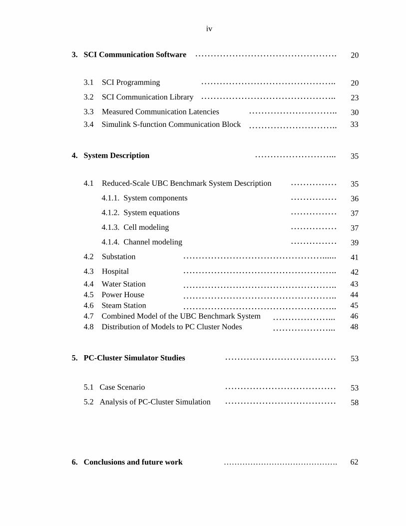
3. SCI Communication Software ………………………………………. 20

3.1 SCI Programming …………………………………….. 20

3.2 SCI Communication Library …………………………………….. 23

3.3 Measured Communication Latencies ……………………….. 30

3.4 Simulink S-function Communication Block ……………………….. 33

4. System Description ……………………... 35

4.1 Reduced-Scale UBC Benchmark System Description …………… 35

4.1.1. System components …………… 36

4.1.2. System equations …………… 37

4.1.3. Cell modeling …………… 37

4.1.4. Channel modeling …………… 39

4.2 Substation ………………………………………...... 41

4.3 Hospital ………………………………………….. 42

4.4 Water Station ………………………………………….. 43 4.5 Power House ………………………………………….. 44 4.6 Steam Station ………………………………………….. 45

4.7 Combined Model of the UBC Benchmark System ………………... 46 4.8 Distribution of Models to PC Cluster Nodes ………………... 48

5. PC-Cluster Simulator Studies ……………………………… 53

5.1 Case Scenario ……………………………… 53

5.2 Analysis of PC-Cluster Simulation ……………………………… 58

6. Conclusions and future work ……………………………………. 62

v

References ……………………………………... 64

Appendix Computer Programs …………………….......................... 69

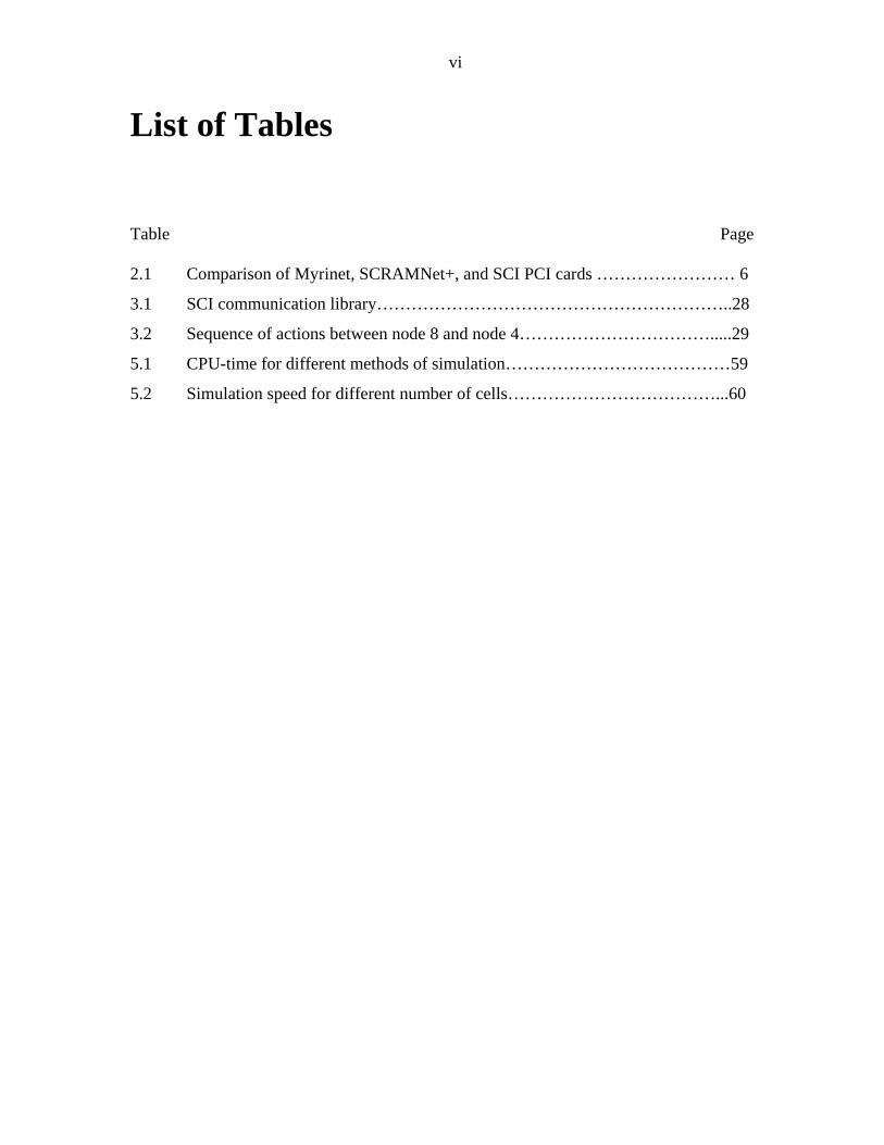
vi

List of Tables Table Page 2.1 Comparison of Myrinet, SCRAMNet+, and SCI PCI cards …………………… 6

3.1 SCI communication library……………………………………………………..28

3.2 Sequence of actions between node 8 and node 4…………………………….....29

5.1 CPU-time for different methods of simulation…………………………………59

5.2 Simulation speed for different number of cells………………………………...60

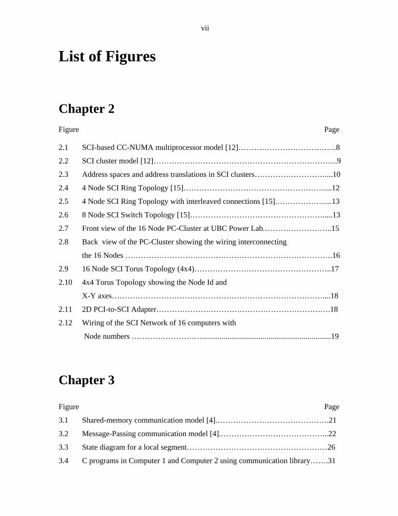
vii

List of Figures

Chapter 2 Figure Page 2.1 SCI-based CC-NUMA multiprocessor model [12]………………………………..8

2.2 SCI cluster model [12]……………………………………………………………..9

2.3 Address spaces and address translations in SCI clusters………………………....10

2.4 4 Node SCI Ring Topology [15]………………………………………………....12

2.5 4 Node SCI Ring Topology with interleaved connections [15].………………....13

2.6 8 Node SCI Switch Topology [15]…………………………………………….....13

2.7 Front view of the 16 Node PC-Cluster at UBC Power Lab.……………………..15

2.8 Back view of the PC-Cluster showing the wiring interconnecting

the 16 Nodes ……………………….…………………………………………….16

2.9 16 Node SCI Torus Topology (4x4)……………………………………………..17

2.10 4x4 Torus Topology showing the Node Id and

X-Y axes………………………………………………………………………....18

2.11 2D PCI-to-SCI Adapter………………………………………………………….18

2.12 Wiring of the SCI Network of 16 computers with

Node numbers ………………………..................................................................19

Chapter 3 Figure Page

3.1 Shared-memory communication model [4].…………………………………….21

3.2 Message-Passing communication model [4].…………………………………...22

3.3 State diagram for a local segment………………………………………………26

3.4 C programs in Computer 1 and Computer 2 using communication library…….31

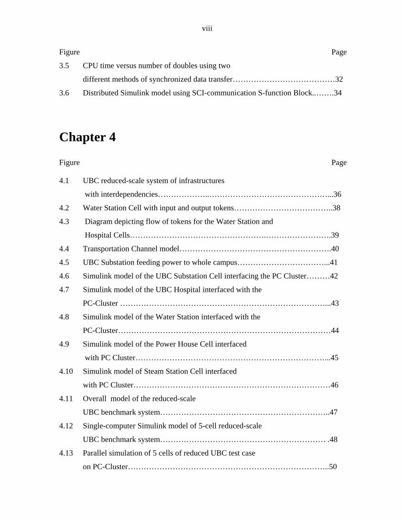
viii

Figure Page

3.5 CPU time versus number of doubles using two

different methods of synchronized data transfer…………………………………32

3.6 Distributed Simulink model using SCI-communication S-function Block..…….34

Chapter 4

Figure Page 4.1 UBC reduced-scale system of infrastructures

with interdependencies………………..………………………………………...36

4.2 Water Station Cell with input and output tokens………………………………..38

4.3 Diagram depicting flow of tokens for the Water Station and

Hospital Cells…………………………………………….…………………….39

4.4 Transportation Channel model………………………………………………….40

4.5 UBC Substation feeding power to whole campus……………………………...41

4.6 Simulink model of the UBC Substation Cell interfacing the PC Cluster………42

4.7 Simulink model of the UBC Hospital interfaced with the

PC-Cluster ……………………………………………………………………...43

4.8 Simulink model of the Water Station interfaced with the

PC-Cluster………………………………………………………………………44

4.9 Simulink model of the Power House Cell interfaced

with PC Cluster………………………………………………………………...45

4.10 Simulink model of Steam Station Cell interfaced

with PC Cluster…………………………………………………………………46

4.11 Overall model of the reduced-scale

UBC benchmark system………………………………………………………..47

4.12 Single-computer Simulink model of 5-cell reduced-scale

UBC benchmark system……………………………………………………… .48

4.13 Parallel simulation of 5 cells of reduced UBC test case

on PC-Cluster…………………………………………………………………..50

ix

Figure Page

4.14 User interface on Computer 1 simulating

the Substation Cell……………………………………………………………...50

4.15 User interface on Computer 2 simulating the Hospital Cell…………………..51

4.16 User interface on Computer 3 simulating

the Water Station Cell …………………………………………………………51

4.17 User interface on Computer 4 simulating

Power House Cell……………………………..................................................52

4.18 User interface on Computer 5 simulating

Steam Station Cell………………………………………………………..……52

Chapter 5 Figure Page 5.1 Electricity token dispatched from

Substation to the Hospital………………………………………………………55

5.2 Electricity token dispatched from

Substation to the Power House………………………………………………....55

5.3 Simulation results for power token dispatch from Power House

to the Water Station…………………………………………………………….56

5.4 Water token dispatch from Water Station to the Hospital……………………...56

5.5 Simulation results for Hospital output tokens in terms of

number of beds in service………………………………………………………57

5.6 Simulation results for steam token output form Steam Station Cell…………...58

5.7 CPU-time for different number of cells with single computer

and distributed simulation……………………………………………………...61

x

Acknowledgements

I would like to acknowledge and thank Dr. Juri Jatskevich for providing me the opportunity

to pursue research in the area of advanced computing technology. I extend my sincere

gratitude for his guidance, encouragement and continuous assistance in this project. I gladly

acknowledge my debt to Dr. Juri Jatskevich and Dr. José R. Martí for the financial assistance

without which it would not have been possible for me to come to Canada for graduate

studies. Dr. Martí has always inspired me with his philosophical discussions, which

expanded my horizon of thinking and creativity. His commendations motivated me to work

hard for achieving the milestones of this project.

I would like to express a token of special appreciation to Power Lab and Joint Infrastructure

Interdependencies Research Program (JIIRP) members particularly, Jorge Hollman, Tom De

Rybel, Marcelo Tomim, Hafiz Abdur Rahman, Lu Liu, Michael Wrinch, and Quanhong Han,

without whom this work could not be accomplished.

I would also like to thank Roy Nordstroem and other members of Dolphin Interconnect

Solutions Inc., Norway, for their help in developing software infrastructure for my project.

I am deeply indebted to my beloved wife, Madhavi, for her unconditional love and moral

support during extreme difficult times in my life which inspired me in pursuit of excellence

in the field of endeavor. I owe my wellbeing and success to her. I am also grateful to my

sons, Aravind and Akhil, for their love and affection even in a situation when I stayed away

from them for long time. I am particularly grateful to my elder son, Aravind, who has

boosted my morale with his thinking and emotional support which were exceptional for his

young age.

UBC, August 2007 Siva Singupuram

xi

To Madhavi, Aravind and Akhil

- 1 -

Chapter 1

Introduction

1.1 Research Motivation

The Joint Infrastructure Interdependencies Research Program (JIIRP) is part of ongoing

national efforts to secure and protect Canadians from natural disasters and terrorist attacks

[1]. Water utilities, communications, banking, transportation networks and hospitals have

many complex interaction points and depend critically on each other to function properly.

The interdependencies issue has only recently been recognized as a key factor for optimal

decision making where the ultimate outcome of the JIIRP is to produce new knowledge-

based practices to better assess, manage, and mitigate risks to the lives of Canadians [2]. The

system interactions are complex and dynamic. Simulation of complex heterogeneous systems

for coordinated decision making in the case of emergency situations such as an earth quake

or a terrorist attack requires an intensive computational tool. Advance performance

forecasting of the constituent elements and the system as a whole, is highly essential. This

requires that many simulations are run very quickly to find the optimal solution – a sequence

of mitigating actions. The development of a monitor to intuitively visualize and comprehend

the information on the system dynamics for anticipation of incipient emergencies by the

human operators, leads to many research challenges including powerful computing. If the

simulation of complex systems is done on a single computer, the physical computing time

(the CPU time) can be prohibitively long. In spite of continuous increase in the

computational capability of computers, the need to model complex infrastructure systems at

increasingly higher levels of detail to study their interrelationships makes the computing time

a critical issue. This kind of computationally intensive simulation can be successfully done

using a PC-Cluster simulator. The development and implementation of PC-Cluster based

simulator is the subject of this thesis.

- 2 -

1.2 Related Work

In the domain of infrastructure modeling, numerous works and studies have focused on the

modeling, simulation and analysis of single entity elements. Few projects, however, have

attempted to combine multiple-infrastructure networks into one model with the specific

intent of analyzing the interactions and interdependencies between the systems. The efforts

are being made by Idaho National Engineering and Environment Laboratory (INEEL) to

implement parallel simulation for infrastructure modeling at the Idaho Nuclear Technology

and Engineering Center (INTEC) to study potential vulnerabilities, emergent behaviours

from infrastructure outages, and to assist in the development of protective strategies [3]. The

Message Passing Interface (MPI) was used to parallelize the code and facilitate the

information exchange between processors [4]. However, the paradigm of computer

networking used therein introduces a significant communication overhead leading to slower

simulation speed. This limits the study of interdependencies of complex networks where

large amount of data exchange between the processors would take place. To achieve low

communication latency of the order of micro-seconds, one of the few available interconnect

standards such as the Scalable Coherent Interface (SCI) [ANSI/IEEE Std 1596-1992) can be

adopted [5].

1.3 System Interconnection Network

System interconnection networks have become a critical component of the computing

technology of the late 1990s, and they are likely to have a great impact on the design,

architecture, and the use of future high-performance computers. Not only the sheer

computational speed but also the efficient integration of the computing nodes into tightly

coupled multiprocessor system that distinguishes high performance clusters from desktop

systems. Network adapters, switches, and device driver software are increasingly becoming

performance critical components in modern supercomputers.

Due to the recent availability of fast commodity network adapter cards and switches, tightly

integrated clusters of PCs or workstations can be built, to fill the gap between desktop

- 3 -

systems and supercomputers. These PC-Clusters can be used to perform powerful

computation wherein independent tasks can be executed in parallel. The use of commercial

off-the-shelf (COTS) technology for both computing and networking enables scalable

computing at relatively low costs. Some may disagree, but even the world champion in high-

performance computing, Sandia Lab’s Accelerated Strategic Computing Initiative (ASCI)

Red Machine [6], may be seen as COTS system. Clearly the system area network plays a

decisive role in overall performance.

1.4 Contributions

An approach of achieving a high simulation speed for complex infrastructures is to distribute

the whole system over different computers in a system area network using fast network

adapters connection that perform the simulation concurrently. Then, these computers can

communicate with each other back and forth implementing the interdependencies among the

relevant subsystems. As the CPU resource of any one computer is limited, implementing

simulations on multi-computer networks offers considerable potential for reducing the

overall computing time. However, in a PC-Cluster based simulation, additional time will be

required to communicate the data between the computers.

This project represents an important milestone in the quest of a fast computing tool for

complex simulations. A novel approach of building a PC-Cluster based simulator via high-

speed Scalable Coherent Interface (SCI) network adaptor cards has been proposed,

implemented and discussed in this thesis. In this research a 16 nodes PC-Cluster is developed

using Dolphin SCI Adapter Cards [7]. The most suitable topology, including other topologies

for networking is discussed and implemented. Next a communication library of user callable

functions has been developed, in order to use the Dolphin SCI Adapter Card and the

associated low-level functions [8]. Different interrupt mechanisms are investigated for back

and forth synchronized data transfer. To reduce the communication overhead between the

cluster nodes, a new interrupt mechanism has been developed and implemented. A user

defined block, based on the communication libraries is developed in MATLAB/SIMULINK

- 4 -

[9], to communicate between different processors. It is shown that an improvement of

computational speed over a single computer can be achieved through parallelism using the

SCI-based PC-Cluster. For the considered benchmark system, an increase in simulation

speed of up to 5 times was achieved.

1.5 Composition of the Thesis

This thesis is outlined as follows. In Chapter 2, the concepts of system area network and

point-to-point links of SCI adapter cards are presented. Several network topologies are

examined. Based on preliminary review of SCI-based networks, a specific architecture for

building the PC-Cluster at the UBC Power Lab is described that is best suited to accomplish

the research objectives. Next, in Chapter 3, possible software protocols are examined and

suitable low level functions are chosen to build the communication library of user callable

functions. The communication latencies between two nodes of the SCI-based PC-Cluster are

measured for different interrupt mechanisms of synchronized data transfer. A

MATLAB/SIMULINK S-function block is developed for communicating between

SIMULINK models in different nodes. The SIMULINK model of an interdependent reduced-

scale UBC benchmark system of infrastructures is implemented and described in Chapter 4.

In Chapter 5, the simulation studies and results are compared with those obtained from a

conventional single processor implementation. The conclusions are summarized in Chapter 6,

which also includes suggestions for the future research.

- 5 -

Chapter 2

SCI-Based PC-Cluster

Scalable Coherent Interface (SCI) is an innovative interconnect standard (ANSI/IEEE Std

1596-1992 [1]) that addresses the high performance computing and networking domain. SCI

is used as a high-speed interconnection network (often called system area network) for

compute clusters built from commodity workstation nodes. In this chapter, several

communication networks for distributed simulations are described and compared

qualitatively and quantitatively. SCI Interconnect, System Area Network for Clusters, Point-

to-Point Link, and various network topologies evaluated and discussed. Finally the hardware

infrastructure of 16 nodes UBC Power lab PC-Cluster is presented.

2.1 Communication Networks

Over the years, numerous communication networks and concepts have been proposed for

building clusters or tightly-coupled multiprocessors like NUMA (non-uniform memory

access) or CC-NUMA (cache coherent non-uniform memory access) systems. The

Myricom’s Myrinet [2] is a high-speed system area and local area network that has its origins

in the interconnect technology of a massively parallel machine. Network interface cards

attaching to workstations’ I/O buses, high-speed links, switches, and a wealth of software,

predominantly optimized message-passing libraries, are available to facilitate the

construction of high performance compute clusters. In contrast to SCI, a shared address space

across the nodes in a cluster is not provided by the technology. However, the adapter card

hosts a programmable processor, which allows specific communication mechanisms to be

implemented, among them abstractions emulating the distributed shared memory (DSM [3]).

Also the network cost is relatively high because Myrinet requires crossbar switches for

network connection [4].

- 6 -

SCRAMNet+ (Shared Common Random Access Memory Network) from Curtis-Wright

Controls Embedded Computing (CWCEC) [5] is another cluster interconnects that supports

high-bandwidth and low data latency. The SCRAMNet+ approach is a shared-memory

network that has a common pool of memory accessible from multiple nodes through PCI

cards. The software for Windows NTTM or Linux is commercially available; however, the

software must be purchased for each node.

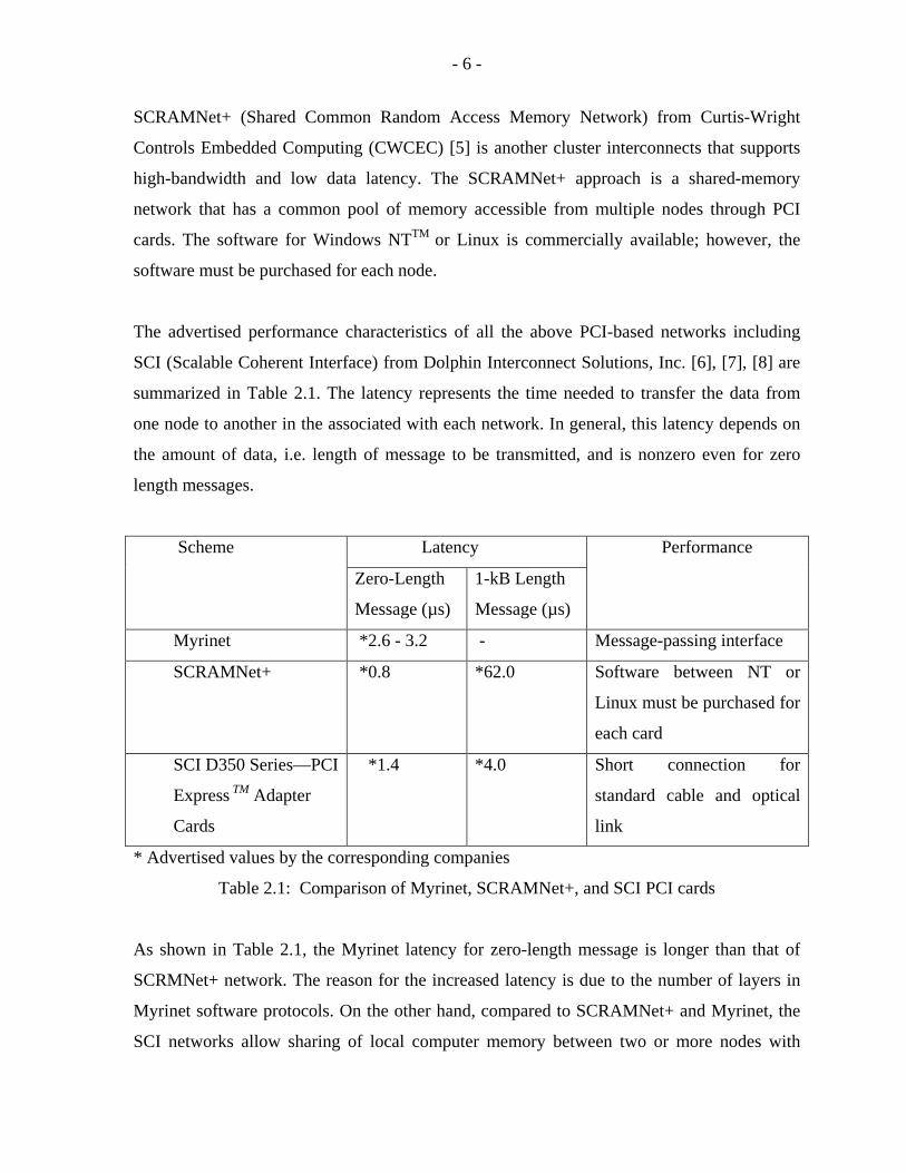
The advertised performance characteristics of all the above PCI-based networks including

SCI (Scalable Coherent Interface) from Dolphin Interconnect Solutions, Inc. [6], [7], [8] are

summarized in Table 2.1. The latency represents the time needed to transfer the data from

one node to another in the associated with each network. In general, this latency depends on

the amount of data, i.e. length of message to be transmitted, and is nonzero even for zero

length messages.

Latency Scheme

Zero-Length

Message (µs)

1-kB Length

Message (µs)

Performance

Myrinet *2.6 - 3.2 - Message-passing interface

SCRAMNet+ *0.8 *62.0 Software between NT or

Linux must be purchased for

each card

SCI D350 Series—PCI

Express TM Adapter

Cards

*1.4 *4.0 Short connection for

standard cable and optical

link

* Advertised values by the corresponding companies

Table 2.1: Comparison of Myrinet, SCRAMNet+, and SCI PCI cards

As shown in Table 2.1, the Myrinet latency for zero-length message is longer than that of

SCRMNet+ network. The reason for the increased latency is due to the number of layers in

Myrinet software protocols. On the other hand, compared to SCRAMNet+ and Myrinet, the

SCI networks allow sharing of local computer memory between two or more nodes with

- 7 -

relatively low latencies. Moreover, the SCI software for NT and Linux is freely distributed.

In this project, D350 Series – SCI-PCI Express TM adapter card [9] was selected because of

its advertised low communication latency, low price per card, and the fact that it can be used

to implement either shared-memory or message-passing programming paradigms, thus

offering more options and future flexibility for the UBC Cluster than other network cards.

Features and benefits of the Dolphin PCI-SCI networks [10] include:

• Dolphin PCI-SCI is ANSI/IEEE 1596-1992 scalable and coherent interface

compliant.

• Currently, the SCI software supports Linux, Windows NTTM, Lynx and Solaris

operating systems.

• It is possible to communicate on an SCI cluster using different operating systems on

different nodes, for example between Windows NTTM and Linux.

• The SCI supports multiprocessing with very low latency and high data throughput.

• The SCI reduces the delay of inter-processor communication by an enormous factor

compared to the newest and best interconnect technologies that are based on

generation of networking and I/O protocols (Fiber Channel and ATM), because SCI

eliminates the run-time layers of software protocol-paradigm translation [11].

2.2 SCI Interconnect

The use of SCI as a cache-coherent memory interconnects allows nodes to be tightly

coupled. This application requires SCI to be attached to the memory bus of a node, as

shown in Figure 2.1 [12]. At this attachment point, SCI can participate in and “export”, if

necessary, the memory and cache coherence traffic on the bus and make the node’s

memory visible and accessible to other nodes. The nodes’ memory address ranges (and the

address mappings of processes) can be laid out to span a global (virtual) address space,

giving processes transparent and coherent access to memory anywhere in the system.

Typically this approach is adopted to connect multiple-bus-based commodity SMPs

(symmetric multiprocessors) to form a large-scale, cache-coherent (CC) shared-memory

system, often termed a CC-NUMA (cache-coherent non-uniform memory access) machine.

- 8 -

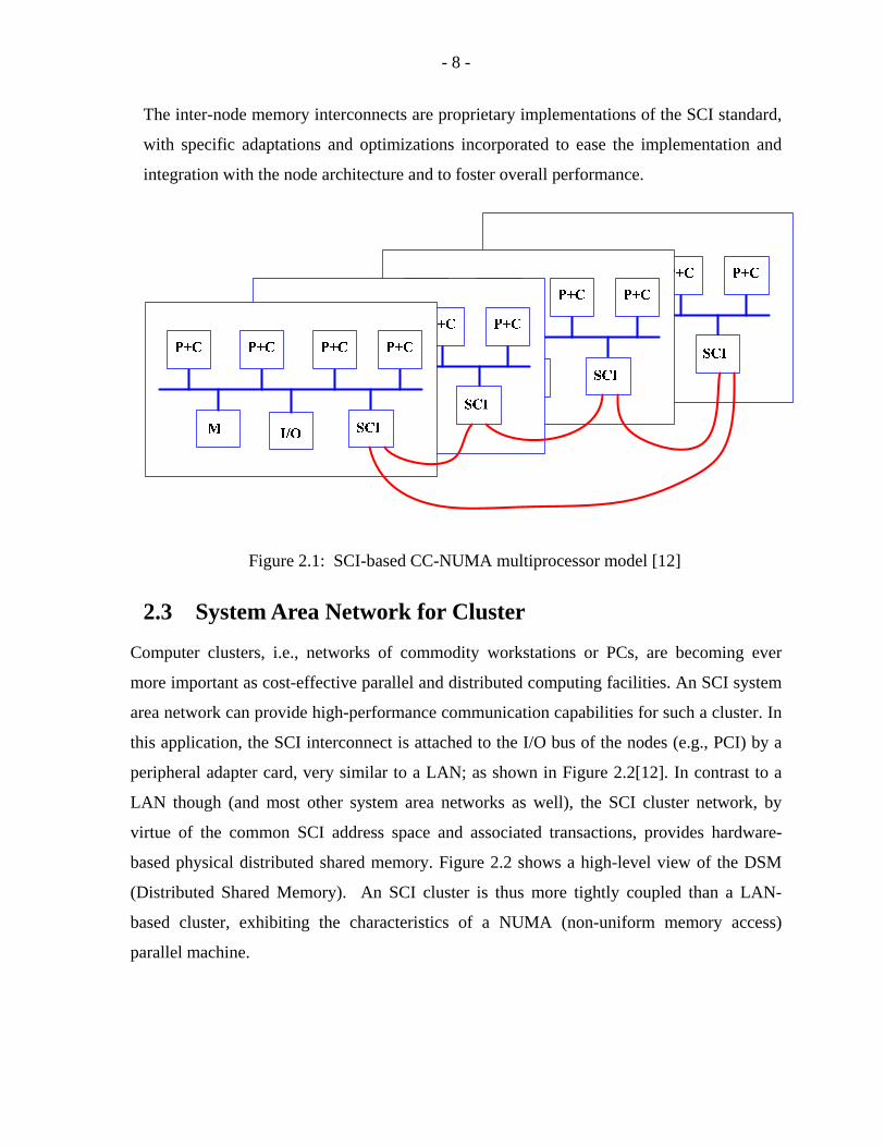
The inter-node memory interconnects are proprietary implementations of the SCI standard,

with specific adaptations and optimizations incorporated to ease the implementation and

integration with the node architecture and to foster overall performance.

Figure 2.1: SCI-based CC-NUMA multiprocessor model [12]

2.3 System Area Network for Cluster

Computer clusters, i.e., networks of commodity workstations or PCs, are becoming ever

more important as cost-effective parallel and distributed computing facilities. An SCI system

area network can provide high-performance communication capabilities for such a cluster. In

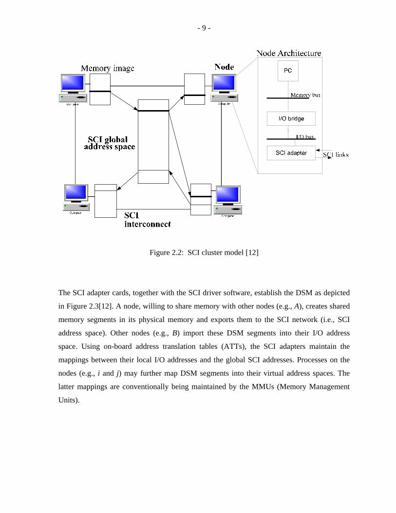
this application, the SCI interconnect is attached to the I/O bus of the nodes (e.g., PCI) by a

peripheral adapter card, very similar to a LAN; as shown in Figure 2.2[12]. In contrast to a

LAN though (and most other system area networks as well), the SCI cluster network, by

virtue of the common SCI address space and associated transactions, provides hardware-

based physical distributed shared memory. Figure 2.2 shows a high-level view of the DSM

(Distributed Shared Memory). An SCI cluster is thus more tightly coupled than a LAN-

based cluster, exhibiting the characteristics of a NUMA (non-uniform memory access)

parallel machine.

- 9 -

Figure 2.2: SCI cluster model [12]

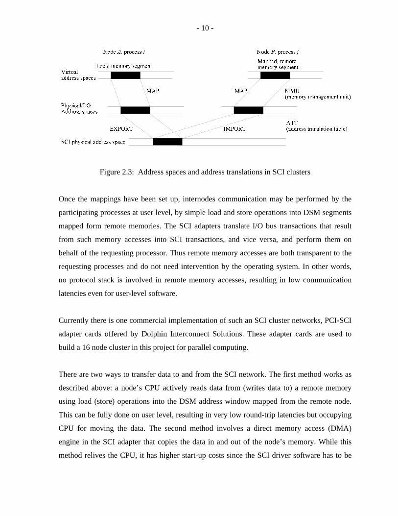
The SCI adapter cards, together with the SCI driver software, establish the DSM as depicted

in Figure 2.3[12]. A node, willing to share memory with other nodes (e.g., A), creates shared

memory segments in its physical memory and exports them to the SCI network (i.e., SCI

address space). Other nodes (e.g., B) import these DSM segments into their I/O address

space. Using on-board address translation tables (ATTs), the SCI adapters maintain the

mappings between their local I/O addresses and the global SCI addresses. Processes on the

nodes (e.g., i and j) may further map DSM segments into their virtual address spaces. The

latter mappings are conventionally being maintained by the MMUs (Memory Management

Units).

- 10 -

Figure 2.3: Address spaces and address translations in SCI clusters

Once the mappings have been set up, internodes communication may be performed by the

participating processes at user level, by simple load and store operations into DSM segments

mapped form remote memories. The SCI adapters translate I/O bus transactions that result

from such memory accesses into SCI transactions, and vice versa, and perform them on

behalf of the requesting processor. Thus remote memory accesses are both transparent to the

requesting processes and do not need intervention by the operating system. In other words,

no protocol stack is involved in remote memory accesses, resulting in low communication

latencies even for user-level software.

Currently there is one commercial implementation of such an SCI cluster networks, PCI-SCI

adapter cards offered by Dolphin Interconnect Solutions. These adapter cards are used to

build a 16 node cluster in this project for parallel computing.

There are two ways to transfer data to and from the SCI network. The first method works as

described above: a node’s CPU actively reads data from (writes data to) a remote memory

using load (store) operations into the DSM address window mapped from the remote node.

This can be fully done on user level, resulting in very low round-trip latencies but occupying

CPU for moving the data. The second method involves a direct memory access (DMA)

engine in the SCI adapter that copies the data in and out of the node’s memory. While this

method relives the CPU, it has higher start-up costs since the SCI driver software has to be

- 11 -

involved to set up the DMA transfer. As we will be using low level data transfer in this

project, the previous method is preferred.

An important property of such SCI cluster interconnect adapters is worth pointing out here.

Since an SCI cluster adapter attaches to the I/O bus of a node, it cannot directly observe, and

participate in, the traffic on the memory bus of the node. This therefore precludes caching

and coherence maintenance of memory regions mapped to the SCI address space. In other

words, remote memory contents are basically treated as non-cacheable and are always

accessed remotely. Therefore, the SCI cluster interconnect hardware doesn’t implement

cache coherence capabilities. Note that this property raises a performance concern: remote

accesses (round-trip operations such as reads) must be used judiciously since they are still an

order of magnitude more expensive than local memory accesses.

The basic approach to deal with the latter problem is to avoid remote operations that are

inherently round-trip, i.e., read, as rare as possible. Rather remote writes are used which are

typically buffered by the SCI adapter and therefore, from the point of view of processor

issuing the write, experience latencies in the range of local accesses, which are several times

faster than remote read operations.

2.4 Point-to-Point Links

An SCI interconnect is defined to be built only from unidirectional, point-to-point links

between participating nodes. These links can be used for concurrent data transfers, in contrast

to the one-at-a-time communications characteristics of buses. The number of links grows as

the nodes are added to the system, increasing the aggregate bandwidth of the network. The

links can be made fast and their performance can scale with the improvements in the

underlying technology.

Most implementations today use parallel links over distances of up to few meters. The data

transfer rates and lengths of shared buses are inherently limited due to signal propagation

delays and signaling problems on the transmission lines, such as capacitive loads that have to

- 12 -

be driven by the sender, impedance mismatches, and noise and signal reflections on the lines.

The unidirectional Point-to-Point SCI links avoid these signalling problems. High speeds are

also fostered by low-voltage differential signals.

Furthermore, SCI strictly avoids back-propagating signals; even reverse flow control on the

links, in favor of high signalling speeds and scalability. A reverse flow control signal would

make timing of, and buffer space required for, a link dependent on the link’s distance [13].

Thus flow control information becomes part of the normal data stream in the reverse

direction, leading to the requirement that an SCI node must at least have one outgoing link

and one incoming link. The SCI cards include two unidirectional links where each speeds

500 Mbytes/s in system area networks (distances of a few meters) [14].

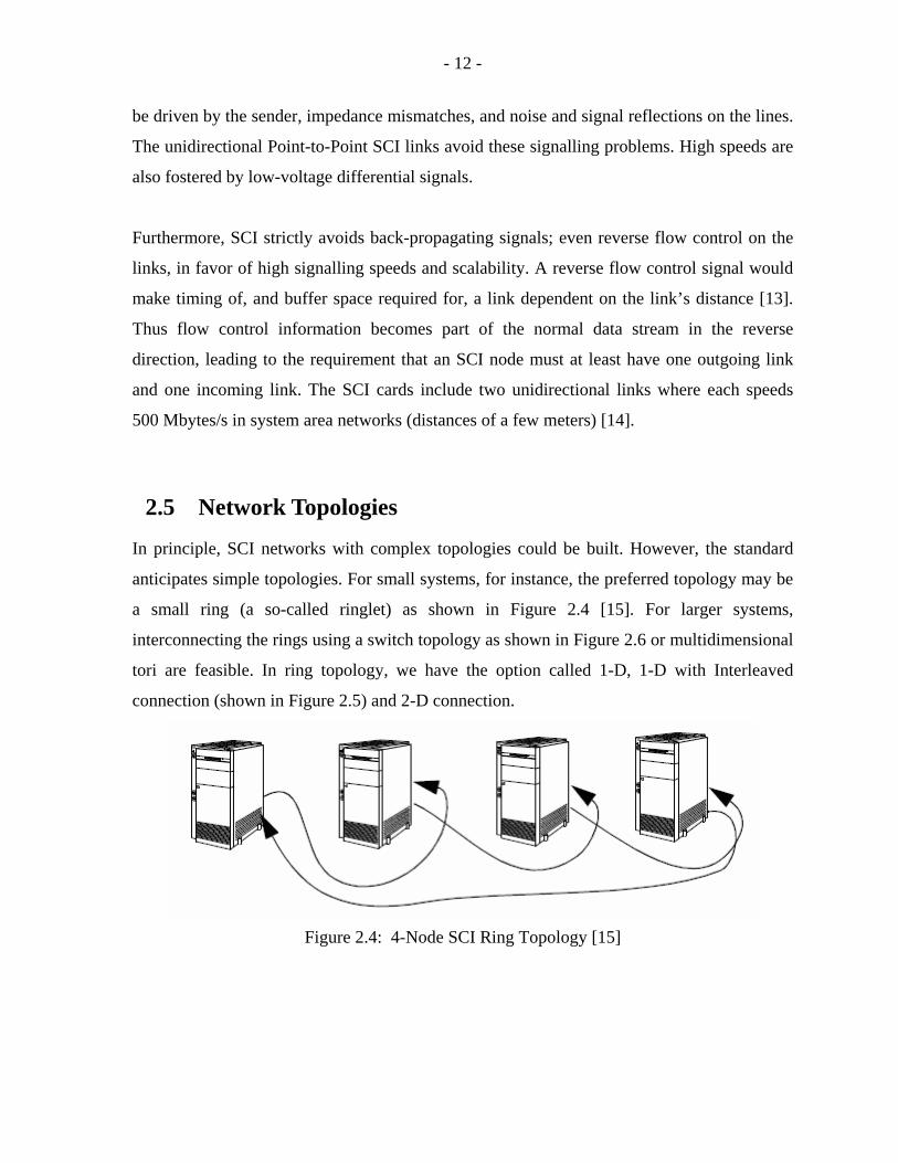
2.5 Network Topologies

In principle, SCI networks with complex topologies could be built. However, the standard

anticipates simple topologies. For small systems, for instance, the preferred topology may be

a small ring (a so-called ringlet) as shown in Figure 2.4 [15]. For larger systems,

interconnecting the rings using a switch topology as shown in Figure 2.6 or multidimensional

tori are feasible. In ring topology, we have the option called 1-D, 1-D with Interleaved

connection (shown in Figure 2.5) and 2-D connection.

Figure 2.4: 4-Node SCI Ring Topology [15]

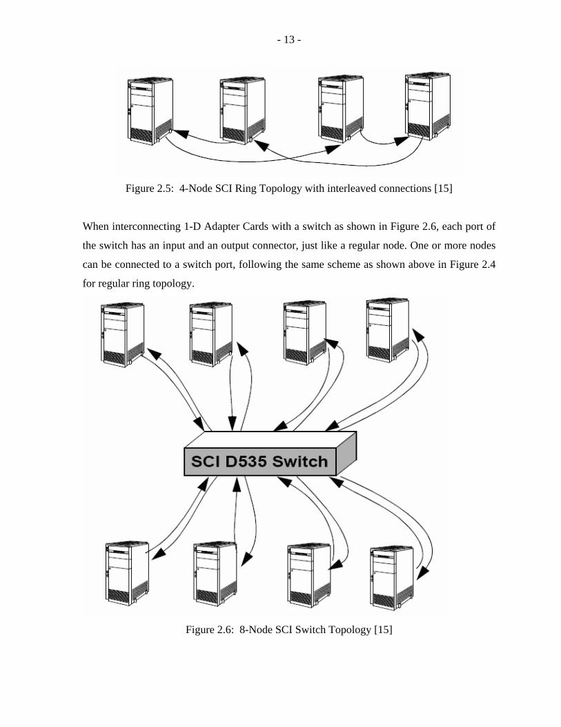
- 13 -

Figure 2.5: 4-Node SCI Ring Topology with interleaved connections [15]

When interconnecting 1-D Adapter Cards with a switch as shown in Figure 2.6, each port of

the switch has an input and an output connector, just like a regular node. One or more nodes

can be connected to a switch port, following the same scheme as shown above in Figure 2.4

for regular ring topology.

Figure 2.6: 8-Node SCI Switch Topology [15]

- 14 -

As explained above, the SCI offers considerable flexibility in topology choices all based on

the fundamental structure of a ring. However, since a message from one node in a ring must

traverse every other node in that ring, this topology becomes inefficient as the number of

nodes increases. Multi-dimensional topologies and/or switches are used to minimize the

traffic paths and congestion in larger systems [15]. The multi-dimensional topologies assume

an equal number of nodes in each dimension. Therefore, for a system with D-dimensions and

n nodes in each dimension, the total number of nodes (i.e. system size) is equal to nD. With

simple ring, all nodes must share a common communication path, thus limiting the

scalability. Hence in this project the two dimensional torus topology (4x4) is considered to

achieve optimum performance from the latency perspective.

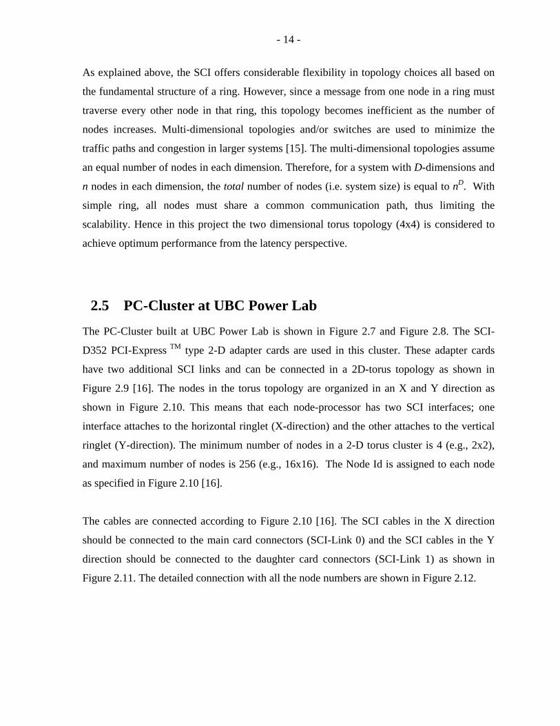
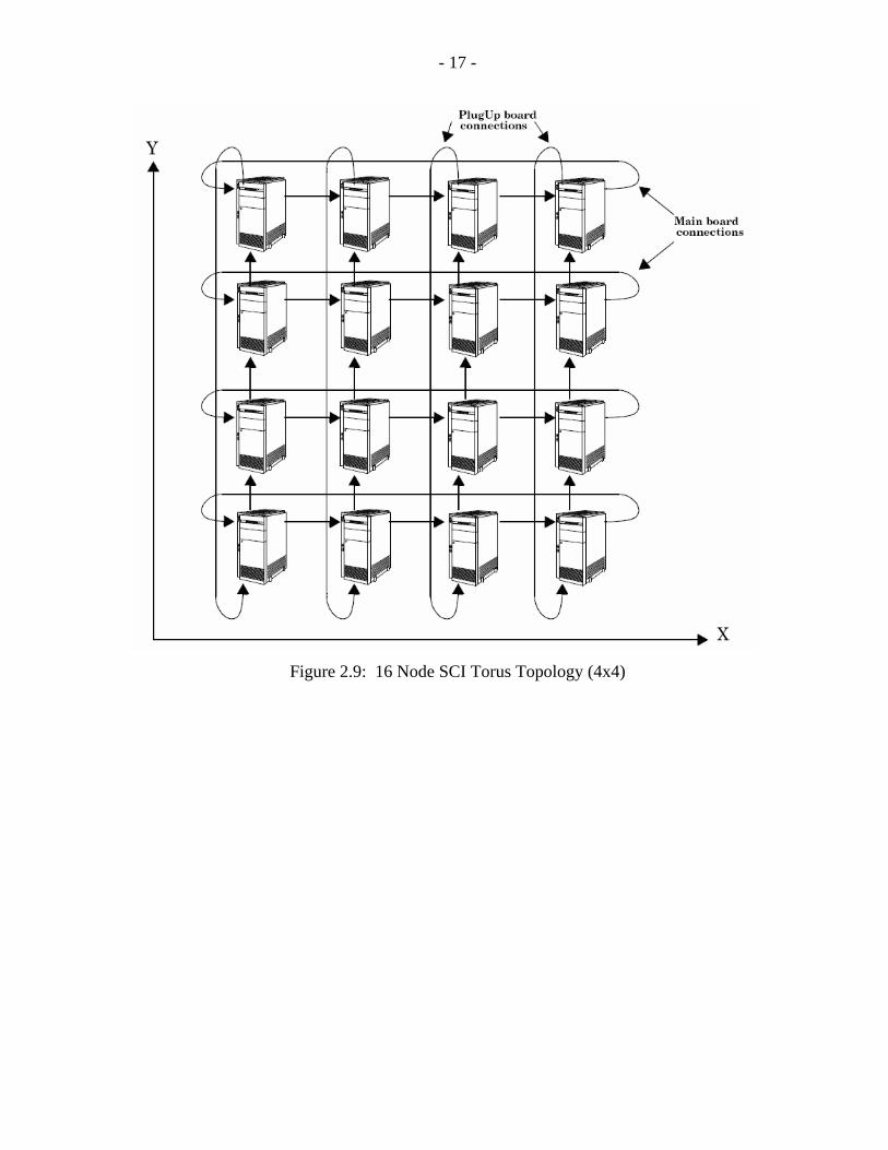
2.5 PC-Cluster at UBC Power Lab

The PC-Cluster built at UBC Power Lab is shown in Figure 2.7 and Figure 2.8. The SCI-

D352 PCI-Express TM type 2-D adapter cards are used in this cluster. These adapter cards

have two additional SCI links and can be connected in a 2D-torus topology as shown in

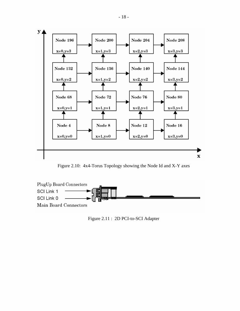
Figure 2.9 [16]. The nodes in the torus topology are organized in an X and Y direction as

shown in Figure 2.10. This means that each node-processor has two SCI interfaces; one

interface attaches to the horizontal ringlet (X-direction) and the other attaches to the vertical

ringlet (Y-direction). The minimum number of nodes in a 2-D torus cluster is 4 (e.g., 2x2),

and maximum number of nodes is 256 (e.g., 16x16). The Node Id is assigned to each node

as specified in Figure 2.10 [16].

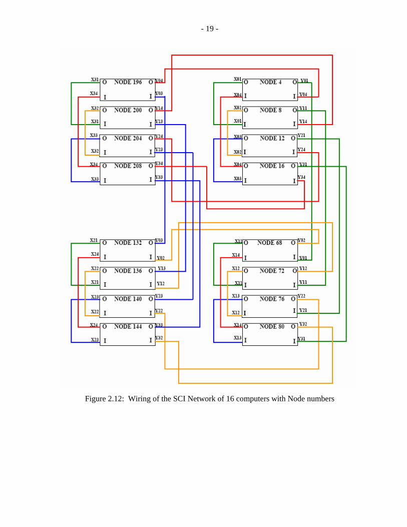
The cables are connected according to Figure 2.10 [16]. The SCI cables in the X direction

should be connected to the main card connectors (SCI-Link 0) and the SCI cables in the Y

direction should be connected to the daughter card connectors (SCI-Link 1) as shown in

Figure 2.11. The detailed connection with all the node numbers are shown in Figure 2.12.

- 15 -

Figure 2.7: Front view of the 16-Node PC-Cluster at UBC Power Lab

- 16 -

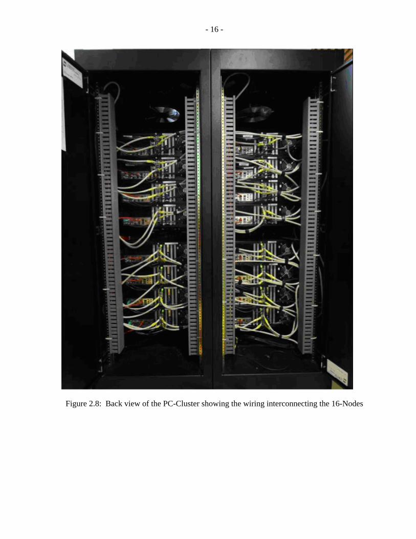
Figure 2.8: Back view of the PC-Cluster showing the wiring interconnecting the 16-Nodes

- 17 -

Figure 2.9: 16 Node SCI Torus Topology (4x4)

- 18 -

Figure 2.10: 4x4-Torus Topology showing the Node Id and X-Y axes

Figure 2.11 : 2D PCI-to-SCI Adapter

- 19 -

Figure 2.12: Wiring of the SCI Network of 16 computers with Node numbers

- 20 -

Chapter 3

SCI Communication Software Regardless of the selected network topology, the SCI standard is designed to support two

main communication software protocols for programming of parallel tasks: Message-Passing

and Shared Address Space. The SCI promises efficient implementation of both paradigms as

it allows transport of messages with extremely low latency and high bandwidth, thus

providing an ideal platform for the message-passing applications. The SCI also provides a

direct access to remote memory using plain load-store transactions, thus providing an equally

good base for the shared memory applications. In this chapter, the trade-offs between both

programming protocols are briefly discussed. The fastest low-level functions [1] are chosen

to develop a libraries composed of set of user-callable communication routines in order to

implement the distributed simulation using PC-Cluster. The communication latencies for

different interrupt mechanisms of synchronized data transfer are measured and compared.

Additionally, the MATLAB/SIMULINK [2] S-function block has been developed to

facilitate communication between SIMULINK models residing on different cluster nodes.

3.1 SCI Programming

The IEEE SCI standard [3] defines a shared memory interconnect from the physical layer to

the transport layer. However, no standard user-callable software layer is defined. In a

distributed shared memory environment, little software is required because once a distributed

shared memory (DSM) system is set up all accesses can be performed by directly

reading/writing from/to the appropriate shared memory spaces. It results in the lowest

possible message passing latency and transaction overhead. No procedures or system services

need to be called in order to exchange data between system nodes. Although there is no

software required to perform DSM data exchange, there is a fair amount of software

infrastructure necessary to create an appropriate shared memory segment and to export it into

- 21 -

the global shared address space or to import that global shared memory segment into the

local address space of another process.

Transaction overhead and latency are very important features in complex distributed

simulations, where distributed shared memory systems are widely used. Therefore the

software interface standard for DSM (distributed shared memory) applications was designed

in such a way that it does implement all necessary hardware abstraction functions but avoids

any additional functionality that would increase the overhead.

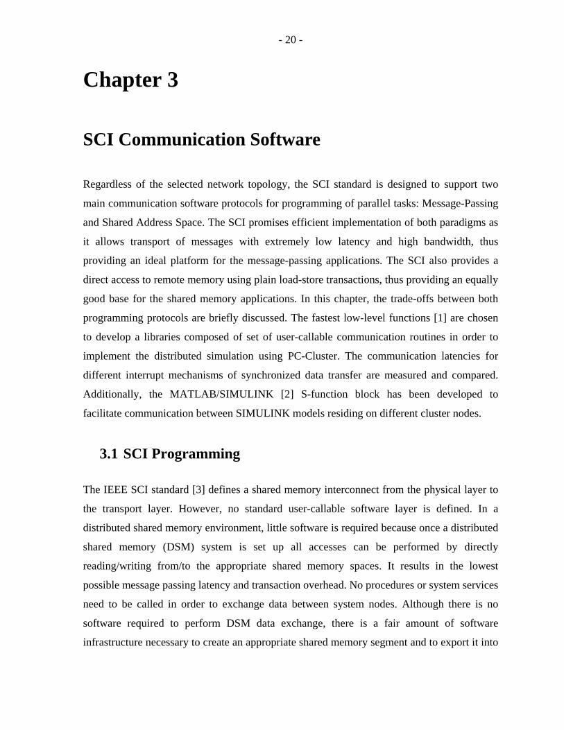
In the shared-memory protocol, all the processors in the network share a global memory as

shown in Figure 3.1[4]. The SCI DSM constitutes a shared physical address space only,

disallowing caching of remote memory contents. It is much more challenging to devise and

realize shared-memory or shared-objects abstractions in this environment than it is to

implement message passing-programming models. The major challenge involved is to

provide a global virtual address space that can be conveniently and efficiently accessed by

processes or threads distributed in the cluster. Solutions will also have to address caching and

consistency aspects of shared memory models.

Figure 3.1: Shared-memory communication model [4]

- 22 -

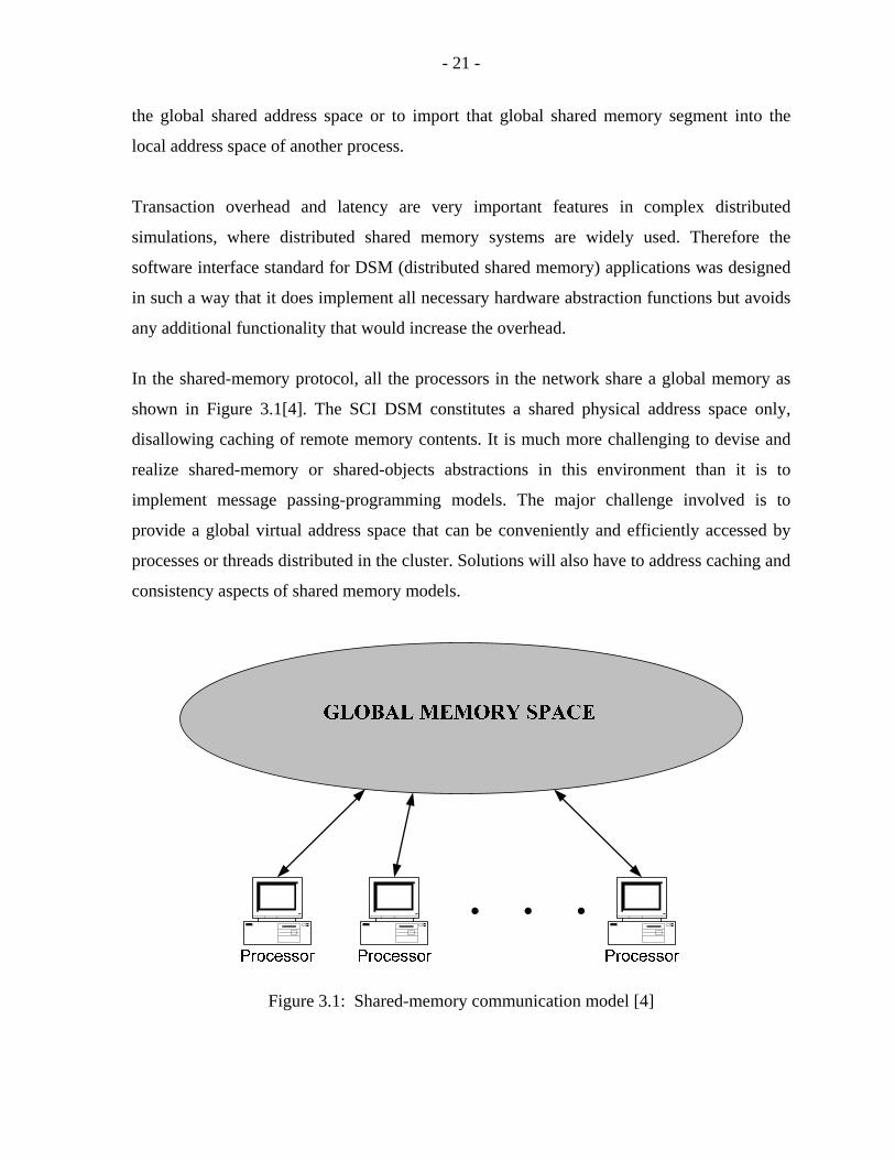
For simplicity reason, message passing communication model as shown in Figure 3.2 [4] is

often used. Message-passing programming requires to explicitly coding of communication

operations. In doing so, it is often simpler to take care of the performance aspects [5]. In this

approach, each processor has its own address space and can only access a location in its own

memory. The interconnection network enables the processors to send messages to other

processors. Also special mechanisms are not necessary in message-passing protocol for

controlling simultaneous access to data, thus reducing the computational overhead of a

parallel program.

The Dolphin adapter cards allow direct mapping of memory accesses from the I/O bus of a

machine to the I/O bus and into the memory of a target machine. This means that the memory

in a remote node can be directly accessed by the CPU using store/load operations giving the

possibility to bypass the time consuming driver calls in the applications. The high latency of

accessing the remote memory as compared to local memory does not make it very attractive

to share the program variable over the SCI, since maintaining cache coherence is not possible

on the I/O bus. A remote CPU read will stall the CPU, but writes are posted such that the

latency is minimized. Message passing model using write-only model fits very well into this

scheme, offering a low-latency, high-bandwidth and reliable channel that makes it possible to

implement an efficient message passing software interface. Thus message-passing method is

adopted in this research because of its straightforward program structure.

Figure 3.2: Message-Passing communication model [4]

- 23 -

3.2 SCI Communication Library

To allow different hardware and software implementations, the IEEE Std P1596.9 “Physical

layer Application Programming Interface (API) for the Scalable Coherent Interface (SCI

PHY-API)” [6] defines an API to abstract the underlying SCI physical layer. An EU-funded

project, named “Standard Software Infrastructures for the SCI-based Parallel Systems”

(SISCI) [7] developed highly advanced state-of-the-art software environment and tools to

exploit the unique hardware capabilities of the SCI communications. The SISCI API [8]

supports:

� Distributed shared memory (DSM) whereby memory segment can be allocated on

one node and mapped in the virtual address space of a process running on another

node. Data is then moved using programmed I/O.

� DMA (Direct Memory Access) transfers to move data from one node to another

without CPU intervention.

� Remote interrupt whereby a process can trigger interrupts on a remote node.

� Fault tolerance allowing a process to check if a transfer was successful and to catch

asynchronous events (such as link failures) and take appropriate actions.

The low-level SCI software functional specifications were developed by Espirit Project

23174 [1]. This project (Software Infrastructure for SCI, “SISCI”) has defined a common

Application Programming Interface to serve as a basis for porting major applications to

heterogeneous multi vendor SCI platforms. However, from the requirement analysis [9] it has

appeared clear that a unique API for all applications is not realistic.

The functional specification of the API is defined in ANSI C [10]. The following

functionality of this SCI API are used here [9].

� Mapping a memory segment residing on a remote node in read/write mode

� Transferring data from remote node via DMA (Direct Memory Access)

� Transferring data to a remote node via DMA

� Getting some information about the underlying SCI system

- 24 -

� Sending an interrupt to an application running on a remote node

� Checking if a function execution failed and why

� Checking data transmission errors

� Transferring data to/from a remote node in a blocking way

� Transferring data to/from a remote node in a non-blocking way

� Sending and receiving raw SCI packets

� All functions are thread-safe

� The API implementation doesn’t deteriorate the characteristic performance of the

SCI technology (high bandwidth and low-latency)

� Implementing API on more than one platform and making SCI network to become a

heterogeneous if the connected nodes are different in terms of platform

The mapping operation is in general very complex and needs to be split in several steps.

Basically, when Node A wants to map a memory segment physically residing on Node B, the

following sequence has to take place:

• Node B allocates the segment and, via one of its SCI interface, makes it available to

Node A

• Node A, via one of its SCI interfaces, connects to the memory segment on Node B

and maps it into its own memory

Making a segment available to every other node means essentially mapping this segment to

the SCI address space, in such a way that it is visible to other nodes. Connecting to a segment

is the complementary action and consists mainly in determining the address range of the

segment inside the SCI address space. But it also means maintaining a relationship between

the physical segment and its mapped companion. The connection then appears to be a very

delicate aspect of the above procedure and it could have strong implications on the lower-

level SCI software, i.e. the driver.

Several models can be adopted to abstract the connection management. For the design of SCI

API (SCI Application Programming Interface) two of them have been considered [9]. They

- 25 -

differ mainly in how a connection is identified. In what is called the segment-oriented model,

a connection is identified by three elements: the physical segment, the SCI adapter used by

the creating node, the SCI adapter used by the connecting node. However this doesn’t allow

distinguishing between all the possible connections, for example in the case when two

connections to the same physical memory segments have been performed via the same SCI

adapters. The alternative, on which the other model, called connection-oriented, is based, is

to assign a unique identifier (handle) to a connection, through which the connection can be

referenced.

The connection-oriented model is evidently more flexible, but it is also more complex to

manage. For this reason, the design of the API is based at the beginning on the segment-

oriented model. There is however the intention to extend the design and then the

specification towards the connection-oriented model. In particular the memory management

and the connection management are well separated. The procedure described above is then

extended as follows:

• On the creating node, an application first allocates a memory segment

(SCICreateSegment), assigning to it a host-unique identifier, and prepares it to be

accessible by the SCI interface (SCIPrepareSegment). What the preparation means

depends on the platform where the software runs. For example, it could consist of making

the segment contiguous and locked in physical memory. These two operations concern

the memory management aspect of the job.

• Finally, the segment is made available to the external network via one or more SCI

interfaces (SCISetSegmentAvailable). This operation represents the connection

part of the job.

A segment can be made unavailable to new connections

(SCISetSegmentUnavailable) without affecting the already established ones. A

segment can be removed only when it is not used any more (SCIRemoveSegment). If the

segment is still in use, locally or remotely, the remove function fails.

- 26 -

Figure 3.3 shows a diagram with the possible states that a local segment can occupy for each

adapter card and the legal transitions between those states. The state of a local segment can

be thought-of as the set of all possible combinations of the states of all the adapters. The

function SCIRemoveSegment is legal operation from all the states, but it fails if the segment

is still in use.

Figure 3.3: State diagram for a local segment

• On the connecting node, an application first needs to connect to the remote segment via

an SCI interface (SCIConnectSegment) and then it can map it into its own address

space (SCIMapRemoteSegment). The two calls create and initialize respectively the

descriptors sci_remote_segment and sci_map and for each return a reference

handle.

When the segment is not any more in use, it has to be unmapped (SCIUnmapSegment) and

disconnected (SCIDisconnectSegment). On the local node, the creation of a memory

segment does not imply that it is mapped in the address space of the creating process. To do

this, a specific action has to be performed (SCIMapLocalSegment), which also produces

a descriptor of type sci_map. The same type descriptor is used for remote mapped segments.

Once the mapping is established, movement of data to or from the mapped segment is

performed by a normal assignment to or from a memory location falling in the range where

the segment has been mapped in an absolutely transparent way. This also means that there is

no software intervention and the typical SCI performance is untouched [9]. Moreover, in

- 27 -

order to profit from hardware-dependent features, a specific function is provided to copy a

piece of memory to a remote map (SCIMemCopy). This optimized SCI interface is used in

the project to transfer data back and forth between two nodes and achieve low

communication latency.

In order to use the SCI adapter cards and the associated low-level functions [1], a library of

SCI user-callable functions has been developed. These communication functions are

compiled into one static library that can be linked to applications such C-based

MATLAB/Simulink [2] or the Fortran-based languages such as ACSL (Advanced

Continuous Simulation Language) [11] and possibly MicroTran [12]. The developed routines

implement message passing transactions and are summarized in Table 3.1 and Table 3.2.

The first function that must be called in a user program is scistart (). This function

initializes the SCI-library, opens the virtual device and verifies the SCI cards installed on a

node. A unique positive integer handle h is returned by this function represents the first

connection. This handle is the identifier of the node-to-node connection. In case of failure of

virtual device or SCI-library, the handle returned by this function is zero. Next, the function

sciinit () is called with respect to the handle h, local Node ID, remote Node ID, and the

vector size of exchange variables. This function initializes the network connection

corresponding to the handle h, by creating and mapping memory segments and then

connecting to remote segments. After initialization of the network corresponding to handle h,

data can be transferred between the nodes back and forth using two other functions called

scisend () and scireceive (). Once the data transfer is done, the particular network

connection link with handle h can be closed using the function sciend (). This unmaps

and removes the memory segments corresponding to handle h. Finally, the sciclose ()

function is called to close the virtual device on the given Node and free the allocated

resources and thus terminate from the SCI environment.

- 28 -

Function Description

scistart (int *h) Initializes the SCI-library, opens virtual device and returns handle h = zero, in case of failure.

sciinit (int *h, int lnId, int rnId, int vecsize)

Initializes the network connection corresponding to the handle h. lnId – local node ID rnId – remote node ID vecsize – size of the vectors (number of exchange variables in doubles). Last memory segment is reserved for the message(1) to tell the remote node , that the data transfer is done Creates local segment Prepares the local segment Maps the local segment to user space Sets the local segment available to other nodes Connects to remote segment Maps remote segment to user space

scisend (int *h, double *invec, int vecsize)

Transfers data from invec (localBuffer) to remote Map using SCIMemCpy. Also sends interrupt message telling remote node that data transfer is done

scireceive (int *h, double *outvec, int vecsize)

Checks for the interrupt message received from the sending node that transferred the data. Once this message is received, it puts data in outvec, from the localMapAddr.

sciend (int *h) Closes the network connection corresponding to the handle h. Unmaps the remote segment. Disconnects the remote segment. Unmaps the local segment. Removes the local segment.

sciclose () Closes the virtual device and frees the allocated resources.

Table 3.1: SCI communication library

- 29 -

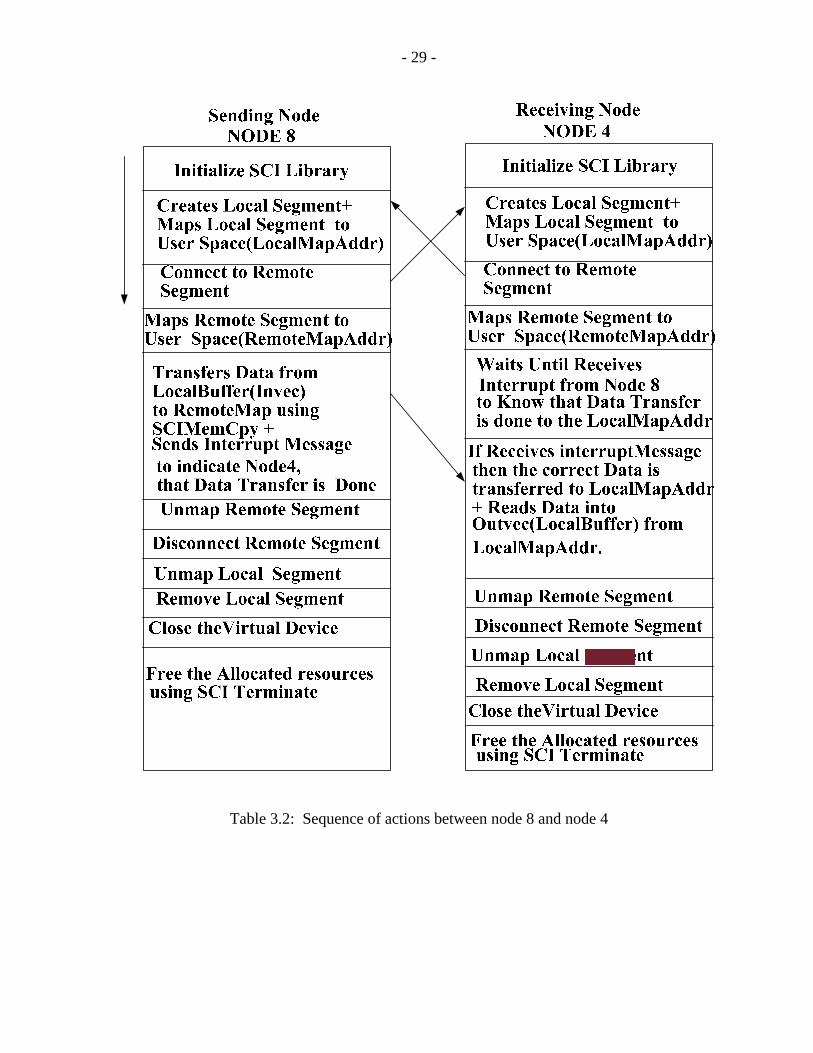
Table 3.2: Sequence of actions between node 8 and node 4

- 30 -

3.3 Measured Communication Latencies

The communication library shown in Table 3.1 can be used in all nodes participating in SCI-

Network. Different interrupt mechanisms can be used to obtain a synchronized data transfer.

This is investigated in this section and the best method for synchronized back and forth data

transfer is used. The communication time between two nodes is measured using the C

programs as described in Figure 3.4.

One possible way is to use interrupt mechanism available in SCI-API (SCI application

programming interface) [1]. It is possible to send and interrupt to an application running on a

remote Node. If an application running on Node A wants to trigger an interrupt for an

application running on Node B, the procedure is the following:

• Application B creates an interrupt resource on its node, assigning to it a host-unique

identifier (SCICreateInterrupt); a descriptor of type sci_local_interrupt_t is

initialized.

• Application A connects to the remote interrupt (SCIConnectInterrupt) that

initializes a descriptor of type (sci_remote_interrupt) and after that, can trigger it

(SCITriggerInterrupt).

When application A does not need any more to trigger, it disconnects from the remote

interrupt (SCIDisconnectInterrupt). Application B frees the interrupt resource with

SCIRemoveInterrupt. Application B can catch the interrupt either specifying a call-back

function at creation time or using a blocking wait function (SCIWaitForInterrupt).

An alternate method of synchronized data transfer is proposed in this thesis. In the proposed

approach, a special bit message flag in the memory segment of the sending node is used. The

receiving node checks for that message flag bit to determine whether or not a new message

was send. Once the message is received, the data can be accepted into local map address.

This kind of polling method does not involve any low-level SCI-API interrupt functions and

is very fast.

- 31 -

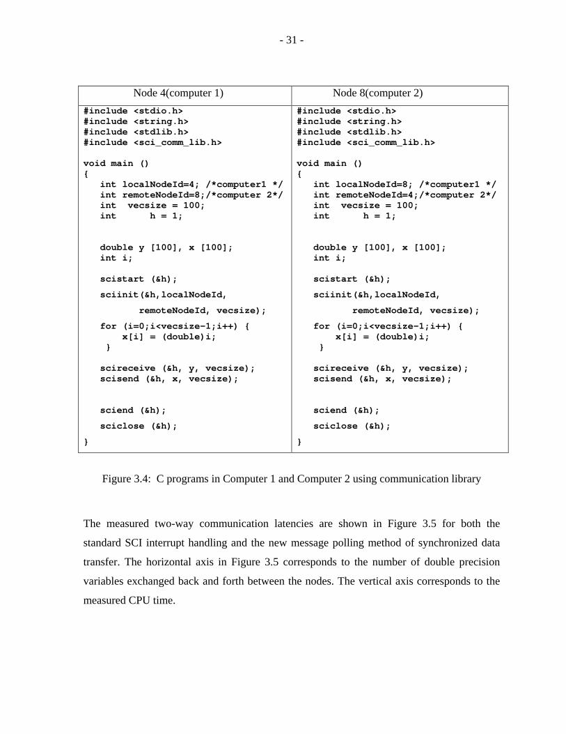
Node 4(computer 1) Node 8(computer 2)

#include <stdio.h> #include <string.h> #include <stdlib.h> #include <sci_comm_lib.h> void main () { int localNodeId=4; /*computer1 */ int remoteNodeId=8;/*computer 2*/ int vecsize = 100; int h = 1; double y [100], x [100]; int i; scistart (&h);

sciinit(&h,localNodeId,

remoteNodeId, vecsize);

for (i=0;i<vecsize-1;i++) { x[i] = (double)i; } scireceive (&h, y, vecsize); scisend (&h, x, vecsize);

sciend (&h);

sciclose (&h);

}

#include <stdio.h> #include <string.h> #include <stdlib.h> #include <sci_comm_lib.h> void main () { int localNodeId=8; /*computer1 */ int remoteNodeId=4;/*computer 2*/ int vecsize = 100; int h = 1; double y [100], x [100]; int i; scistart (&h);

sciinit(&h,localNodeId,

remoteNodeId, vecsize);

for (i=0;i<vecsize-1;i++) { x[i] = (double)i; } scireceive (&h, y, vecsize); scisend (&h, x, vecsize);

sciend (&h);

sciclose (&h);

}

Figure 3.4: C programs in Computer 1 and Computer 2 using communication library

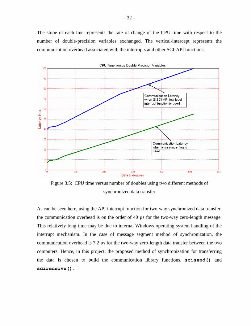
The measured two-way communication latencies are shown in Figure 3.5 for both the

standard SCI interrupt handling and the new message polling method of synchronized data

transfer. The horizontal axis in Figure 3.5 corresponds to the number of double precision

variables exchanged back and forth between the nodes. The vertical axis corresponds to the

measured CPU time.

- 32 -

The slope of each line represents the rate of change of the CPU time with respect to the

number of double-precision variables exchanged. The vertical-intercept represents the

communication overhead associated with the interrupts and other SCI-API functions.

Figure 3.5: CPU time versus number of doubles using two different methods of

synchronized data transfer

As can be seen here, using the API interrupt function for two-way synchronized data transfer,

the communication overhead is on the order of 40 µs for the two-way zero-length message.

This relatively long time may be due to internal Windows operating system handling of the

interrupt mechanism. In the case of message segment method of synchronization, the

communication overhead is 7.2 µs for the two-way zero-length data transfer between the two

computers. Hence, in this project, the proposed method of synchronization for transferring

the data is chosen to build the communication library functions, scisend() and

scireceive().

- 33 -

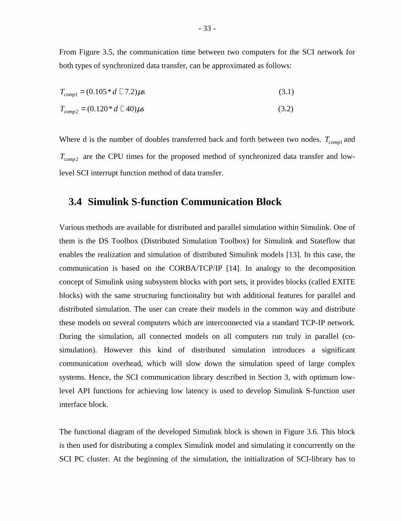
From Figure 3.5, the communication time between two computers for the SCI network for

both types of synchronized data transfer, can be approximated as follows:

sdTcomp µ)2.7*105.0(1 += (3.1)

sdTcomp µ)40*120.0(2 += (3.2)

Where d is the number of doubles transferred back and forth between two nodes. 1compT and

2compT are the CPU times for the proposed method of synchronized data transfer and low-

level SCI interrupt function method of data transfer.

3.4 Simulink S-function Communication Block

Various methods are available for distributed and parallel simulation within Simulink. One of

them is the DS Toolbox (Distributed Simulation Toolbox) for Simulink and Stateflow that

enables the realization and simulation of distributed Simulink models [13]. In this case, the

communication is based on the CORBA/TCP/IP [14]. In analogy to the decomposition

concept of Simulink using subsystem blocks with port sets, it provides blocks (called EXITE

blocks) with the same structuring functionality but with additional features for parallel and

distributed simulation. The user can create their models in the common way and distribute

these models on several computers which are interconnected via a standard TCP-IP network.

During the simulation, all connected models on all computers run truly in parallel (co-

simulation). However this kind of distributed simulation introduces a significant

communication overhead, which will slow down the simulation speed of large complex

systems. Hence, the SCI communication library described in Section 3, with optimum low-

level API functions for achieving low latency is used to develop Simulink S-function user

interface block.

The functional diagram of the developed Simulink block is shown in Figure 3.6. This block

is then used for distributing a complex Simulink model and simulating it concurrently on the

SCI PC cluster. At the beginning of the simulation, the initialization of SCI-library has to

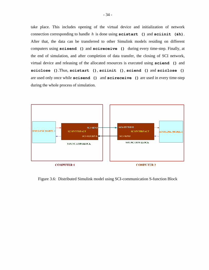
- 34 -

take place. This includes opening of the virtual device and initialization of network

connection corresponding to handle h is done using scistart () and sciinit (&h).

After that, the data can be transferred to other Simulink models residing on different

computers using scisend () and scireceive () during every time-step. Finally, at

the end of simulation, and after completion of data transfer, the closing of SCI network,

virtual device and releasing of the allocated resources is executed using sciend () and

sciclose ().Thus, scistart (), sciinit (), sciend () and sciclose ()

are used only once while scisend () and scireceive () are used in every time-step

during the whole process of simulation.

Figure 3.6: Distributed Simulink model using SCI-communication S-function Block

- 35 -

Chapter 4

System Description It should be acknowledged that development of the infrastructure cell models is an on-going

research mostly carried out by other graduate students working on the JIIRP project in the

UBC Power Lab; whereas the focus of this thesis remains to be software and hardware of the

SCI-based PC-Cluster. In this chapter, a reduced-scale UBC test case for joint infrastructure

interdependencies is briefly described for completeness. The Simulink models of these

infrastructures [1] including the S-function communication block introduced in Chapter 3 are

also presented here. The overall reduced-scale benchmark system will be used in this thesis

for demonstration and evaluation of distributed simulation using the SCI-based PC-Cluster.

4.1 Reduced-Scale UBC Benchmark System Description

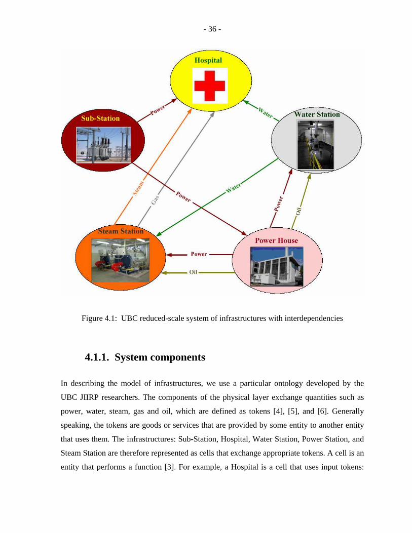
The reduced-scale version of the UBC infrastructures connected with each other form a

complex system shown in Figure 4.1. The five infrastructures include Sub-Station, Hospital,

Water Station, Power House, and Steam Station. This system is selected because it represents

many attributes of a small city [2], which is sufficiently complex to investigate the

improvement in the simulation speed that can be obtained if instead of using a single

computer this system is distributed over 5 computers of the PC-Cluster. For this comparison,

the Simulink models of the infrastructure cells are taken from [1]. The description of a

system of infrastructures requires at least two layers: the physical layer and the human layer

[3]. In this thesis, only the physical layer model has been considered for distributed

simulation.

- 36 -

Figure 4.1: UBC reduced-scale system of infrastructures with interdependencies

4.1.1. System components

In describing the model of infrastructures, we use a particular ontology developed by the

UBC JIIRP researchers. The components of the physical layer exchange quantities such as

power, water, steam, gas and oil, which are defined as tokens [4], [5], and [6]. Generally

speaking, the tokens are goods or services that are provided by some entity to another entity

that uses them. The infrastructures: Sub-Station, Hospital, Water Station, Power Station, and

Steam Station are therefore represented as cells that exchange appropriate tokens. A cell is an

entity that performs a function [3]. For example, a Hospital is a cell that uses input tokens:

- 37 -

electricity, water, medicines, etc. and produces output tokens: e.g., beds served. A group of

one or multiple cells can form a Node. A Node is a Generator Node if the tokens are

produced by its cells or taken out from its storing facilities or exported to other nodes.

Similarly, a Node can be a Load Node if it receives tokens from other nodes and then

delivers to its internal cells for immediate use or storage. In the reduced-scale UBC

benchmark system considered in this thesis, a Node consists of one cell only and it is a

Generator Node with respect to some tokens and at the same time a Load Node with respect

to other tokens. The nodes are connected by the Transportation Channels. The Transportation

Channels are the means by which tokens flow from Generator Node to Load Node. If the

channel is broken down, no tokens can be transmitted through that channel.

4.1.2. System equations

Sometimes in modeling a system where goods are produced and consumed, mathematical

economics concepts are used [7]. In mathematical economics, similar to systems engineering,

the logical relationships between entities and quantities are expressed in terms of

mathematical symbols. Due to the complex problem of representing the dynamics of

infrastructures during the disasters and due to the highly non-linear nature of the underlying

relationships, the mathematical approach is considered to model the system of infrastructures

[3], on which the models used in this thesis are based.

4.1.3. Cell modeling

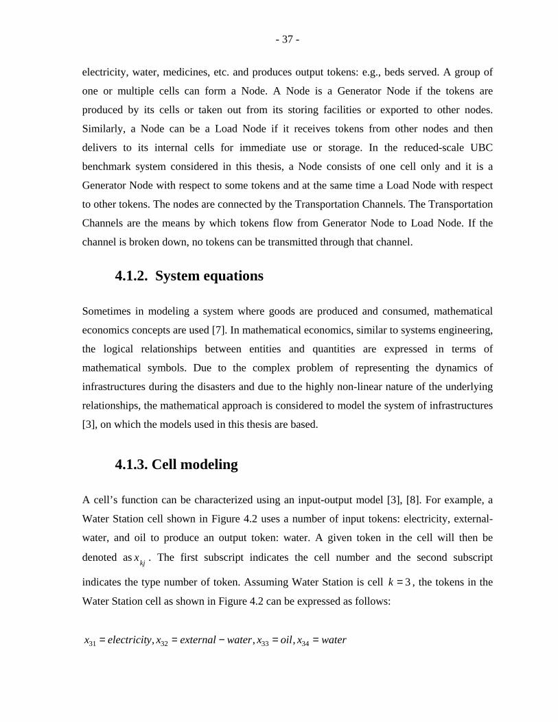
A cell’s function can be characterized using an input-output model [3], [8]. For example, a

Water Station cell shown in Figure 4.2 uses a number of input tokens: electricity, external-

water, and oil to produce an output token: water. A given token in the cell will then be

denoted askj

x . The first subscript indicates the cell number and the second subscript

indicates the type number of token. Assuming Water Station is cell 3=k , the tokens in the

Water Station cell as shown in Figure 4.2 can be expressed as follows:

waterxoilxwaterexternalxyelectricitx ==−== 34333231 ,,,

- 38 -

Figure 4.2: Water Station Cell with input and output tokens

Here it is assumed that the relationship among the tokens can be described by some non-

linear function as:

))(),(),(),(()( 3433323134 txtxtxtxftx = (4.1)

=kjx token j used or produced in k

yelectricitx =31 used

waterexternalx −=32 used

oilx =33 used

waterx =34 produced

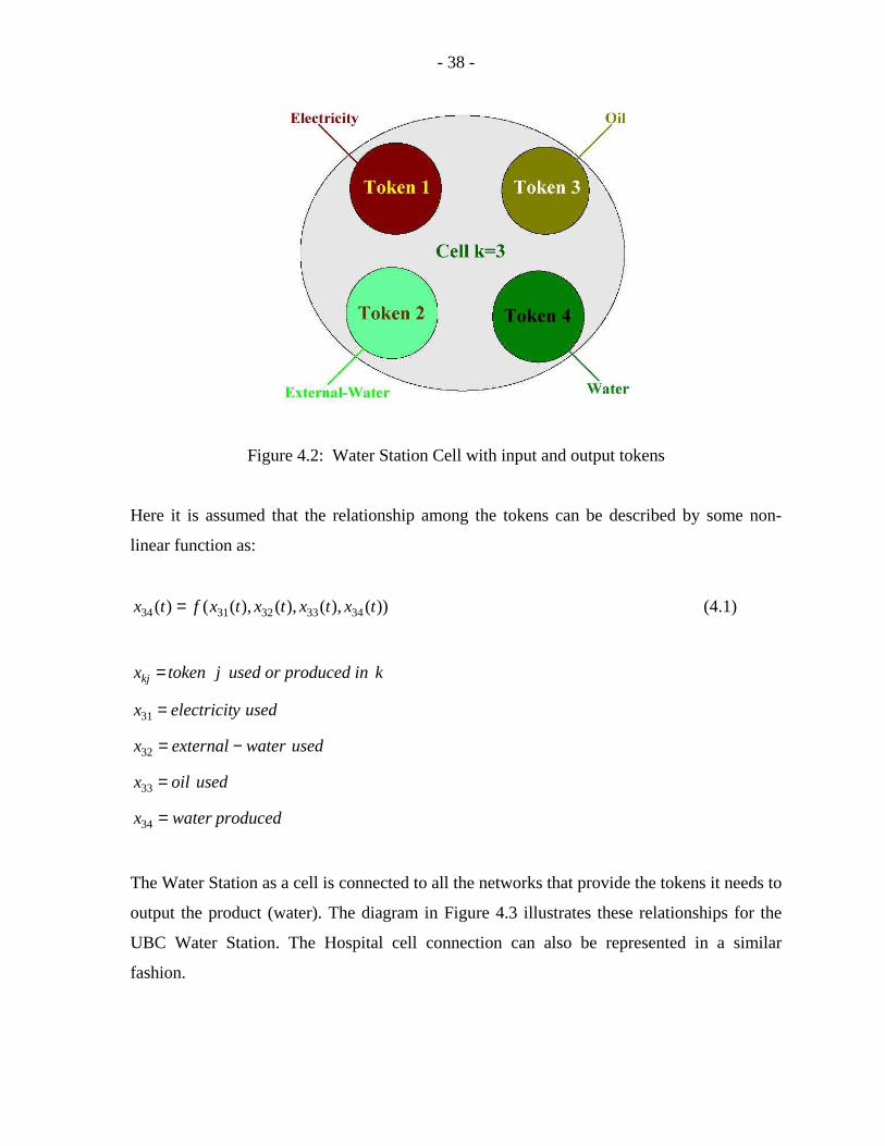
The Water Station as a cell is connected to all the networks that provide the tokens it needs to

output the product (water). The diagram in Figure 4.3 illustrates these relationships for the

UBC Water Station. The Hospital cell connection can also be represented in a similar

fashion.

- 39 -

Figure 4.3: Diagram depicting flow of tokens for the Water Station and Hospital Cells

4.1.4. Channel modeling

In general, the tokens needed at the nodes for the cells to do their jobs come from other nodes

(apart from local storage) [6]. The tokens travel through the transportation network from

Generator Nodes to Load Nodes. A given token may come out of multiple Generator Nodes,

and likewise travel to multiple Load Nodes. Thus, there may be multiple channels linking

Generator Nodes to Load Nodes. For a given Generator Node, dispatching decisions will

determine how the node’s token production will be distributed among the channels coming

out of the node. Once the tokens are in the channels, they may be affected by the channel’s

capacity and transportation delays. How many token units received by a Load Node at a

- 40 -

given instant of time depends on many factors including the amount of token generated in the

system, the dispatching decisions, and the channels capacity and possible delays.

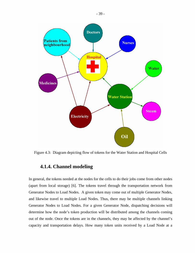
For studying the interdependencies in the UBC benchmark system, specific scenarios can be

implemented using the cell and channels features. For example, the water pipe channel may

be broken and then repaired after sometime during the study [1]. Also, the channels’ gain

may be changed to simulate different capacity of the channels. For example, the channel 32

illustrated in Figure 4.4 [3] is the means for transportation of water from Node 3 to Node 2.

Here, m32 denotes the magnitude and ( )ktD −32 the corresponding time delay. If no water is

lost during the transportation, then 32m becomes 1. Also, if the trip takes 20 minutes

(assuming one time delay is one hour) then

)33.0()( 3232 −= tDtxλ (4.2)

Here subscript stands for “link”. This equations states that the quantity of water arriving at

Node 2 at a given time t is same as the amount of water sent from Node 3 twenty minutes

earlier.

Figure 4.4: Transportation Channel model

The channel model concept is derived from wave propagation in electrical transmission lines

[6]. According to this approach, a wave injected at the sending end of transmission line will

arrive at the receiving end after the elapsed traveling time. The maximum channel capacity

should be considered as a limit in the dispatch block 32D . Broken channels or reduced

capacity links during disaster situations can be modeled easily with the model depicted in

- 41 -

Figure 4.4. For example, if an electric power line has to be disconnected for four hours due to

a fault, the link model for the line would include the transmission line maximum power

capacity plus a delay time of four hours.

4.2 Substation

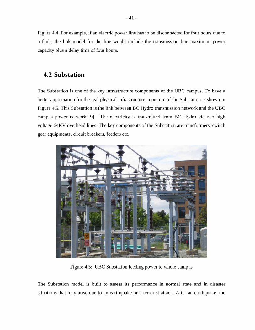
The Substation is one of the key infrastructure components of the UBC campus. To have a

better appreciation for the real physical infrastructure, a picture of the Substation is shown in

Figure 4.5. This Substation is the link between BC Hydro transmission network and the UBC

campus power network [9]. The electricity is transmitted from BC Hydro via two high

voltage 64KV overhead lines. The key components of the Substation are transformers, switch

gear equipments, circuit breakers, feeders etc.

Figure 4.5: UBC Substation feeding power to whole campus The Substation model is built to assess its performance in normal state and in disaster

situations that may arise due to an earthquake or a terrorist attack. After an earthquake, the

- 42 -

Substation service may be deteriorated and require repairs to the damaged components in

order to restore its normal operating condition. The model takes into consideration the

restoration process after the disaster, based on the repairing process as per predefined

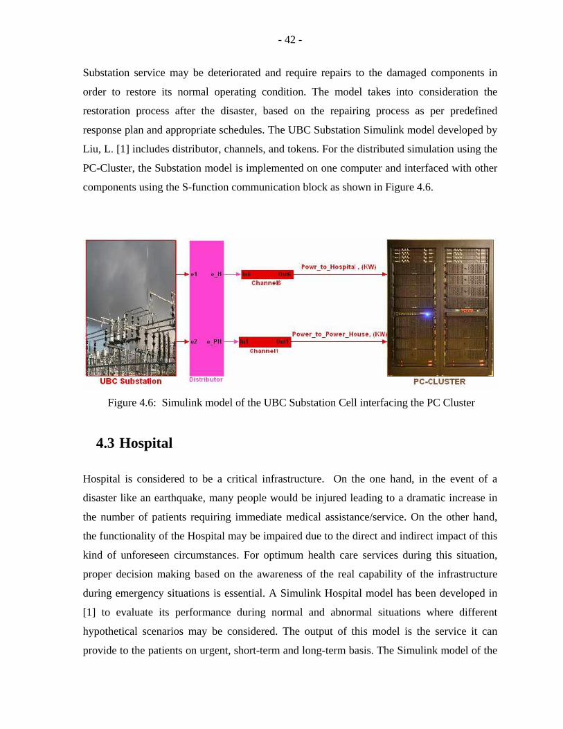
response plan and appropriate schedules. The UBC Substation Simulink model developed by

Liu, L. [1] includes distributor, channels, and tokens. For the distributed simulation using the

PC-Cluster, the Substation model is implemented on one computer and interfaced with other

components using the S-function communication block as shown in Figure 4.6.

Figure 4.6: Simulink model of the UBC Substation Cell interfacing the PC Cluster

4.3 Hospital

Hospital is considered to be a critical infrastructure. On the one hand, in the event of a

disaster like an earthquake, many people would be injured leading to a dramatic increase in

the number of patients requiring immediate medical assistance/service. On the other hand,

the functionality of the Hospital may be impaired due to the direct and indirect impact of this

kind of unforeseen circumstances. For optimum health care services during this situation,

proper decision making based on the awareness of the real capability of the infrastructure

during emergency situations is essential. A Simulink Hospital model has been developed in

[1] to evaluate its performance during normal and abnormal situations where different

hypothetical scenarios may be considered. The output of this model is the service it can

provide to the patients on urgent, short-term and long-term basis. The Simulink model of the

- 43 -

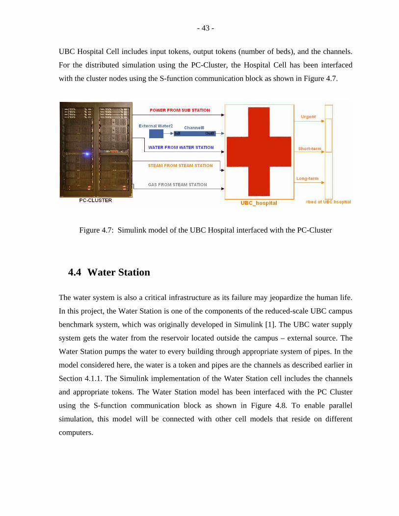
UBC Hospital Cell includes input tokens, output tokens (number of beds), and the channels.

For the distributed simulation using the PC-Cluster, the Hospital Cell has been interfaced

with the cluster nodes using the S-function communication block as shown in Figure 4.7.

Figure 4.7: Simulink model of the UBC Hospital interfaced with the PC-Cluster

4.4 Water Station

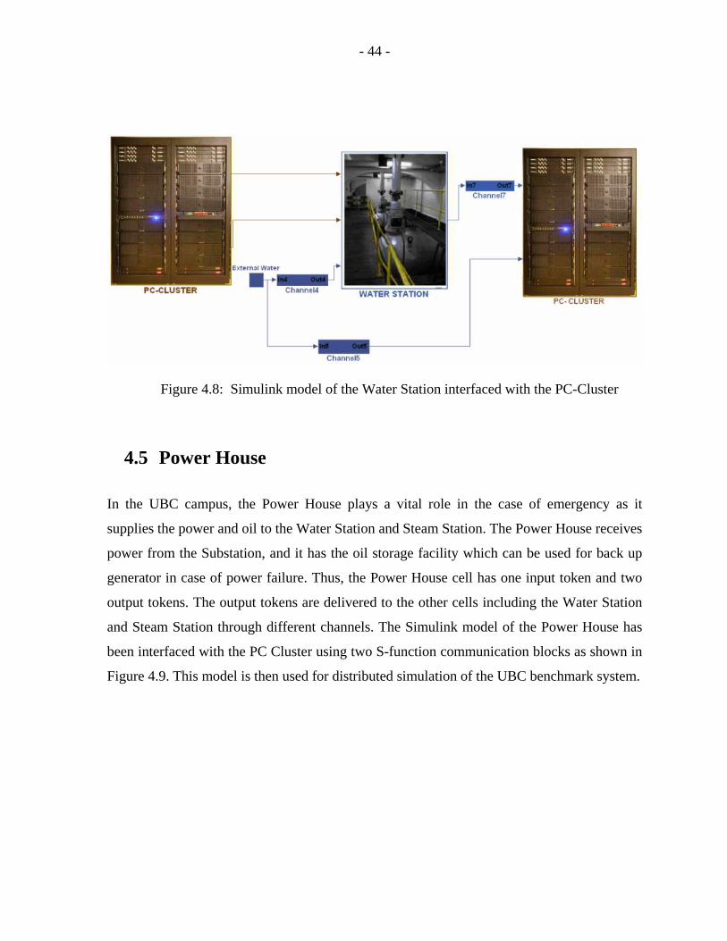
The water system is also a critical infrastructure as its failure may jeopardize the human life.

In this project, the Water Station is one of the components of the reduced-scale UBC campus

benchmark system, which was originally developed in Simulink [1]. The UBC water supply

system gets the water from the reservoir located outside the campus – external source. The

Water Station pumps the water to every building through appropriate system of pipes. In the

model considered here, the water is a token and pipes are the channels as described earlier in

Section 4.1.1. The Simulink implementation of the Water Station cell includes the channels

and appropriate tokens. The Water Station model has been interfaced with the PC Cluster

using the S-function communication block as shown in Figure 4.8. To enable parallel

simulation, this model will be connected with other cell models that reside on different

computers.

- 44 -

Figure 4.8: Simulink model of the Water Station interfaced with the PC-Cluster

4.5 Power House

In the UBC campus, the Power House plays a vital role in the case of emergency as it

supplies the power and oil to the Water Station and Steam Station. The Power House receives

power from the Substation, and it has the oil storage facility which can be used for back up

generator in case of power failure. Thus, the Power House cell has one input token and two

output tokens. The output tokens are delivered to the other cells including the Water Station

and Steam Station through different channels. The Simulink model of the Power House has

been interfaced with the PC Cluster using two S-function communication blocks as shown in

Figure 4.9. This model is then used for distributed simulation of the UBC benchmark system.

- 45 -

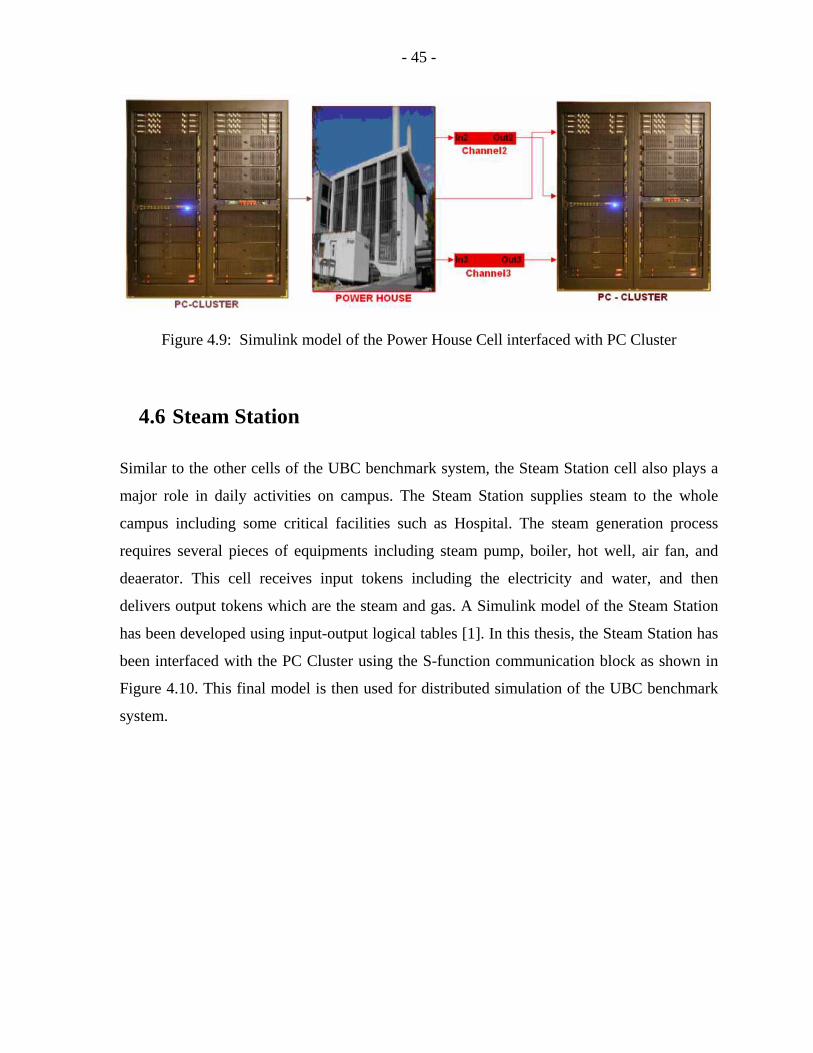
Figure 4.9: Simulink model of the Power House Cell interfaced with PC Cluster

4.6 Steam Station

Similar to the other cells of the UBC benchmark system, the Steam Station cell also plays a

major role in daily activities on campus. The Steam Station supplies steam to the whole

campus including some critical facilities such as Hospital. The steam generation process

requires several pieces of equipments including steam pump, boiler, hot well, air fan, and

deaerator. This cell receives input tokens including the electricity and water, and then

delivers output tokens which are the steam and gas. A Simulink model of the Steam Station

has been developed using input-output logical tables [1]. In this thesis, the Steam Station has

been interfaced with the PC Cluster using the S-function communication block as shown in

Figure 4.10. This final model is then used for distributed simulation of the UBC benchmark

system.

- 46 -

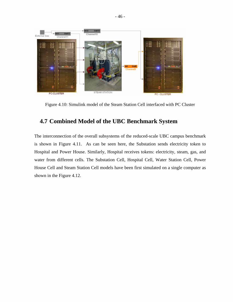
Figure 4.10: Simulink model of the Steam Station Cell interfaced with PC Cluster

4.7 Combined Model of the UBC Benchmark System

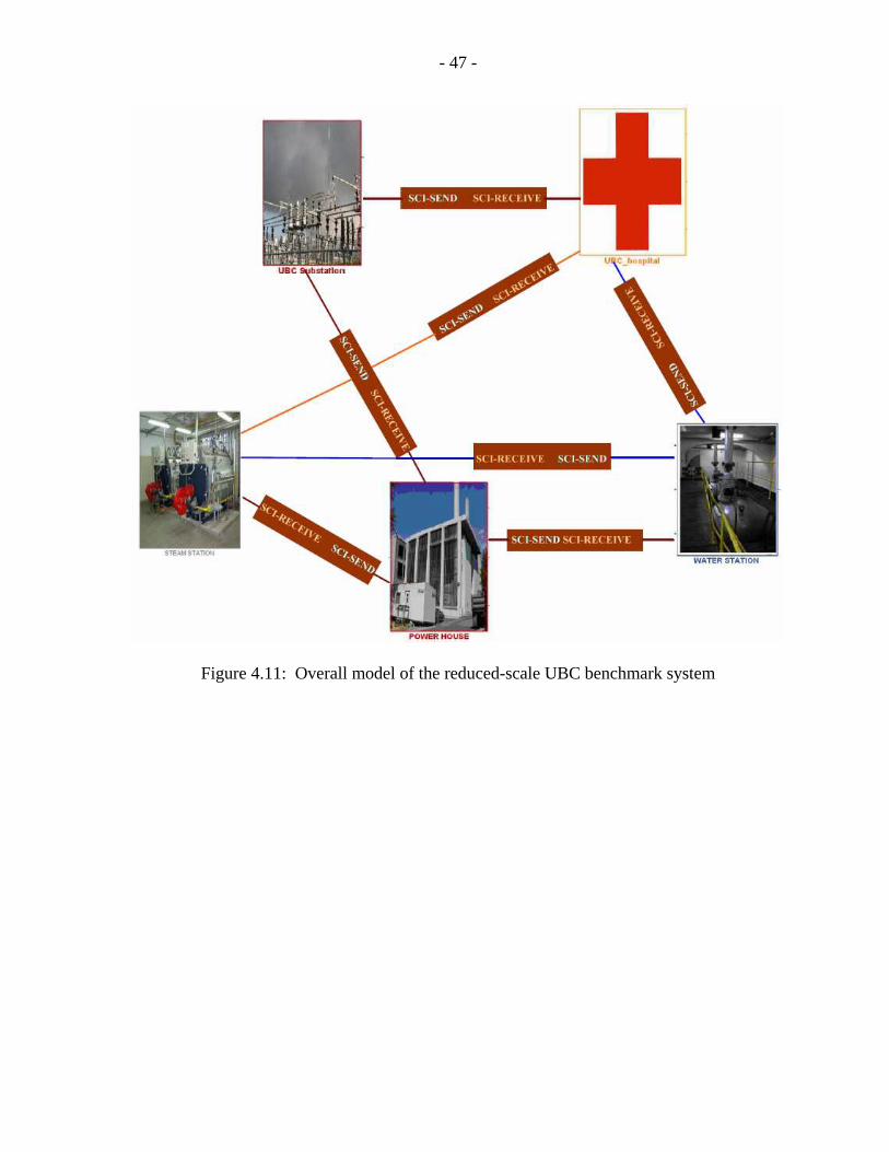
The interconnection of the overall subsystems of the reduced-scale UBC campus benchmark

is shown in Figure 4.11. As can be seen here, the Substation sends electricity token to

Hospital and Power House. Similarly, Hospital receives tokens: electricity, steam, gas, and

water from different cells. The Substation Cell, Hospital Cell, Water Station Cell, Power

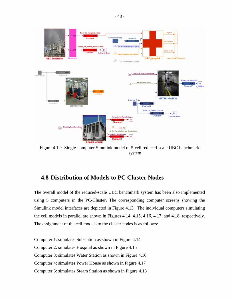
House Cell and Steam Station Cell models have been first simulated on a single computer as

shown in the Figure 4.12.

- 47 -

Figure 4.11: Overall model of the reduced-scale UBC benchmark system

- 48 -

Figure 4.12: Single-computer Simulink model of 5-cell reduced-scale UBC benchmark

system

4.8 Distribution of Models to PC Cluster Nodes

The overall model of the reduced-scale UBC benchmark system has been also implemented

using 5 computers in the PC-Cluster. The corresponding computer screens showing the

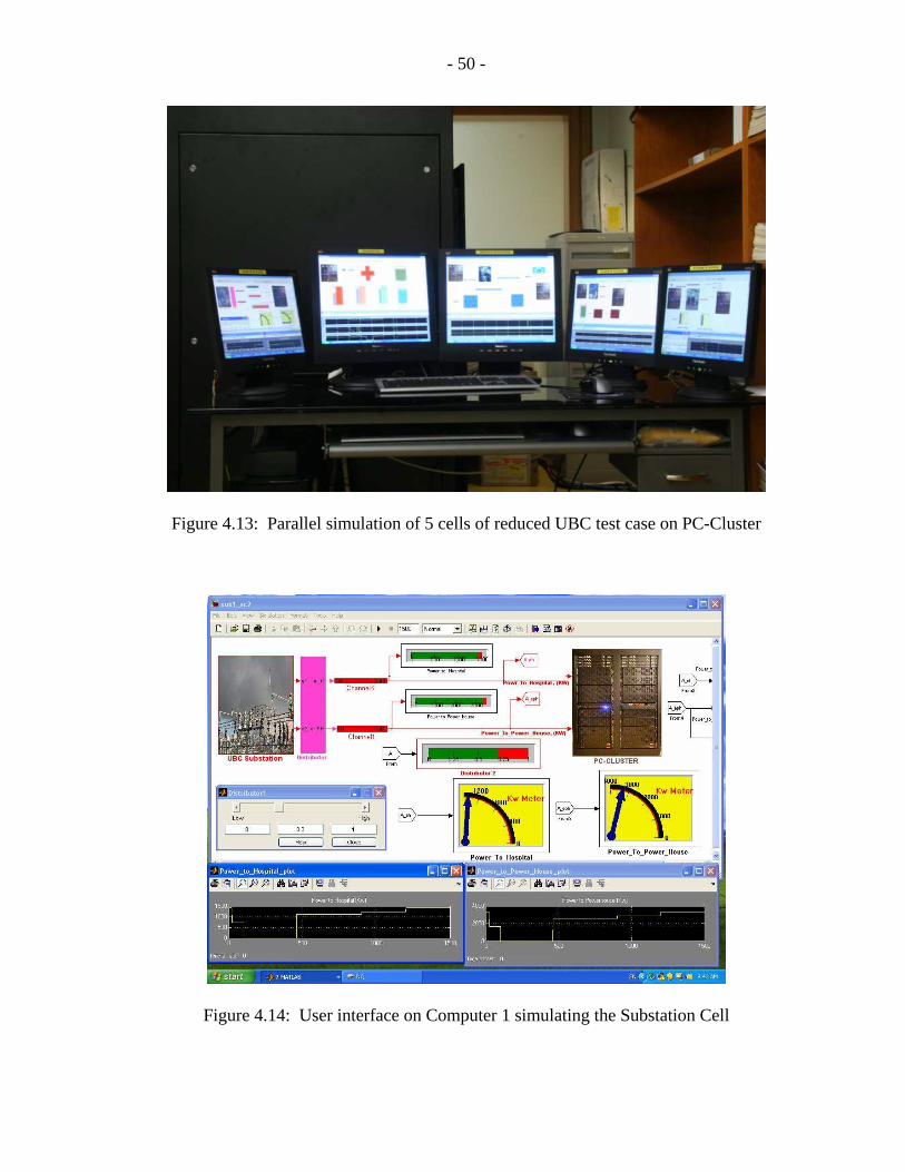
Simulink model interfaces are depicted in Figure 4.13. The individual computers simulating

the cell models in parallel are shown in Figures 4.14, 4.15, 4.16, 4.17, and 4.18, respectively.

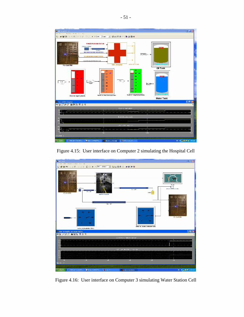
The assignment of the cell models to the cluster nodes is as follows:

Computer 1: simulates Substation as shown in Figure 4.14

Computer 2: simulates Hospital as shown in Figure 4.15

Computer 3: simulates Water Station as shown in Figure 4.16

Computer 4: simulates Power House as shown in Figure 4.17

Computer 5: simulates Steam Station as shown in Figure 4.18

- 49 -

The interdependencies among the cells are realized through the exchange of tokens between

the subsystems, which are implemented using the communication interfaces between the

corresponding cluster nodes. Each cell shown in Figures 4.14 – 4.18 has sophisticated

graphical user interface (GUI) that enables simultaneous monitoring of several variables

and/or tokens during the simulation as well as the user control of the dispatch. This feature is

particularly useful as it allows several users to dynamically interact with the model as the

simulation proceeds and displays the results and flow of the tokens.

The Substation cell in computer 1 receives power token through the transmission line

channels from BC Hydro. Then, it dispatches the electricity token to the Hospital cell in

computer 2 and to the Power House cell in computer 4. The Hospital cell in computer 2

receives 4 tokens: electricity, water, steam and gas from Substation in computer 1, Water

Station in computer 3, and Steam Station in computer 4. Then, the Hospital cell in turn

outputs the services in the form of number of beds serviced for urgent patients, short-term

patients, and long-term patients. The Water Station cell in computer 3 receives water token

from an external source, electricity token from the Power House cell in computer 4, and

outputs water token through water pipe channel to the Hospital in computer 2 and the Steam

Station in computer 5, respectively. The Power House cell in computer 4 gets input

electricity token from Substation in computer 1 and dispatches electricity and oil tokens to

Water Station and Steam Station in computer 3 and computer 5, respectively. Finally, the

Steam Station cell in computer 5 receives electricity token from the Power House and sends

output tokens gas and steam to the Hospital cell in computer 2.

- 50 -

Figure 4.13: Parallel simulation of 5 cells of reduced UBC test case on PC-Cluster

Figure 4.14: User interface on Computer 1 simulating the Substation Cell

- 51 -

Figure 4.15: User interface on Computer 2 simulating the Hospital Cell

Figure 4.16: User interface on Computer 3 simulating Water Station Cell

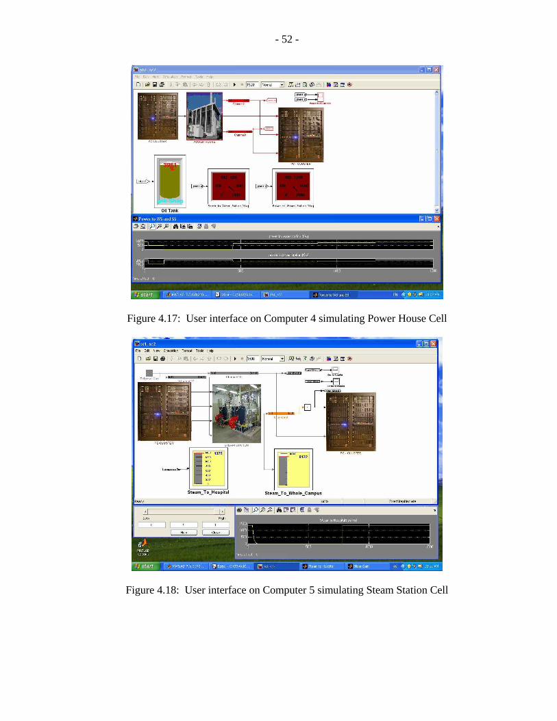
- 52 -

Figure 4.17: User interface on Computer 4 simulating Power House Cell

Figure 4.18: User interface on Computer 5 simulating Steam Station Cell

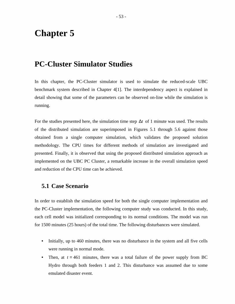
- 53 -

Chapter 5

PC-Cluster Simulator Studies In this chapter, the PC-Cluster simulator is used to simulate the reduced-scale UBC

benchmark system described in Chapter 4[1]. The interdependency aspect is explained in

detail showing that some of the parameters can be observed on-line while the simulation is

running.

For the studies presented here, the simulation time step t∆ of 1 minute was used. The results

of the distributed simulation are superimposed in Figures 5.1 through 5.6 against those

obtained from a single computer simulation, which validates the proposed solution

methodology. The CPU times for different methods of simulation are investigated and

presented. Finally, it is observed that using the proposed distributed simulation approach as

implemented on the UBC PC Cluster, a remarkable increase in the overall simulation speed

and reduction of the CPU time can be achieved.

5.1 Case Scenario

In order to establish the simulation speed for both the single computer implementation and

the PC-Cluster implementation, the following computer study was conducted. In this study,

each cell model was initialized corresponding to its normal conditions. The model was run

for 1500 minutes (25 hours) of the total time. The following disturbances were simulated.

• Initially, up to 460 minutes, there was no disturbance in the system and all five cells

were running in normal mode.

• Then, at 461=t minutes, there was a total failure of the power supply from BC

Hydro through both feeders 1 and 2. This disturbance was assumed due to some

emulated disaster event.

- 54 -

• At 700=t minutes, a disturbance in water supply system was simulated where the

water pipe to the Hospital was broken.

• At 900=t minutes, the power lines were fixed and the normal power was restored.

However, at the same time, irregularities in steam supply to the Hospital were also

created resulting in reduction of the steam production by 50%.

• At 1200=t minutes, the water pipe to the Hospital was repaired and the water supply

was restored to normal. At the same time, the steam supply to the Hospital was

completely cut off to zero.

• At 1400=t minutes, the steam production was finally restored to its nominal

production capacity.

Due to the stated above sequence of disturbances, the situation at the UBC campus unfolded

as follows: From 461=t minutes to 900=t minutes, there was no electricity supply from

Substation to Hospital and Power House as shown in Figure 5.1 and Figure 5.2. Immediately

following this disturbance the backup generators automatically came into service in the

Hospital, Power House and Water Station. As a result of backup generators, there were no

interruptions in the Hospital service for urgent, short-term and long-term patients due to the

failure of power supply from substation as observed in Figure 5.5. However, the disruption in

water supply from Water Station as shown in Figure 5.4, has affected the Hospital service for

30 minutes starting from the time 700=t minutes when the water pipe was broken. After 30

minutes the backup water system came into service and normal operation of the Hospital

service was restored.

However, the disturbance in the Steam Station shown in Figure 5.6 had a greater implication

on the Hospital service. The long-term service was particularly badly affected due to the

interruptions in steam supply. As we can observe when the steam was reduced to 50%, the

long-term beds service was also reduced to half of normal capacity, while urgent- and short-

term patient services were less influenced. In case of complete cut-off of the steam token, the

long-term service was completely unavailable, while sufficient portion of other two types of

beds were still served.

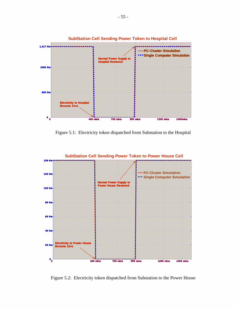
- 55 -

0 0 0 0 460 mins460 mins460 mins460 mins 700 mins700 mins700 mins700 mins 900 mins900 mins900 mins900 mins 1200 mins1200 mins1200 mins1200 mins 1400mins1400mins1400mins1400mins0 0 0 0

500 Kw500 Kw500 Kw500 Kw

1000 Kw1000 Kw1000 Kw1000 Kw

1,417 Kw1,417 Kw1,417 Kw1,417 Kw

PC-Cluster SimulationPC-Cluster SimulationPC-Cluster SimulationPC-Cluster SimulationSingle Computer SimulationSingle Computer SimulationSingle Computer SimulationSingle Computer Simulation

Electricity to HospitalElectricity to HospitalElectricity to HospitalElectricity to HospitalBecame ZeroBecame ZeroBecame ZeroBecame Zero

Normal Power Supply toNormal Power Supply toNormal Power Supply toNormal Power Supply toHospital RestoredHospital RestoredHospital RestoredHospital Restored

SubStation Cell Sending Power Token to Hospital Cell

Figure 5.1: Electricity token dispatched from Substation to the Hospital

0 0 0 0 460 mins460 mins460 mins460 mins 700 mins700 mins700 mins700 mins 900 mins900 mins900 mins900 mins 1200 mins1200 mins1200 mins1200 mins 1400 mins1400 mins1400 mins1400 mins0 0 0 0

20 Kw20 Kw20 Kw20 Kw

40 Kw40 Kw40 Kw40 Kw

60 Kw60 Kw60 Kw60 Kw

80 Kw80 Kw80 Kw80 Kw

100 Kw100 Kw100 Kw100 Kw

120 Kw120 Kw120 Kw120 Kw

139 Kw139 Kw139 Kw139 Kw

PC-Cluster SimulationSingle Computer Simulaiton

Electricity to Power HouseElectricity to Power HouseElectricity to Power HouseElectricity to Power HouseBecame ZeroBecame ZeroBecame ZeroBecame Zero

Normal Power Supply toNormal Power Supply toNormal Power Supply toNormal Power Supply toPower House RestoredPower House RestoredPower House RestoredPower House Restored

SubStation Cell Sending Power Token to Power House Cell

Figure 5.2: Electricity token dispatched from Substation to the Power House

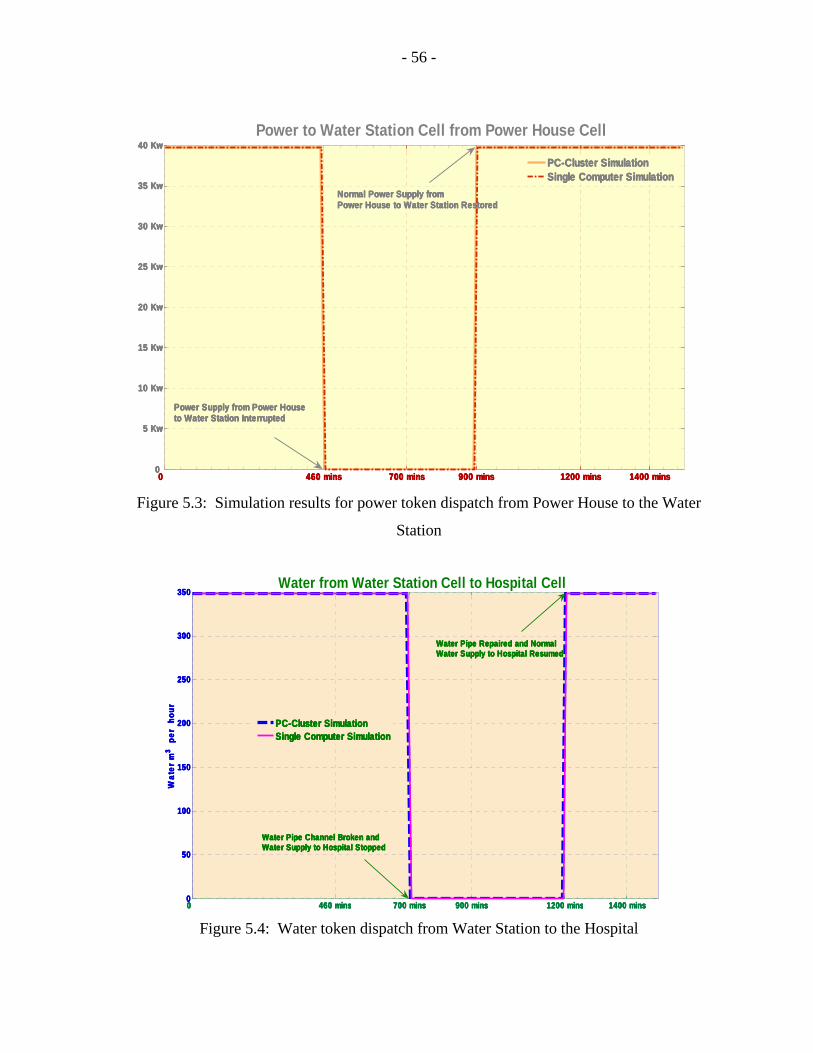
- 56 -

0 0 0 0 460 mins460 mins460 mins460 mins 700 mins700 mins700 mins700 mins 900 mins900 mins900 mins900 mins 1200 mins1200 mins1200 mins1200 mins 1400 mins1400 mins1400 mins1400 mins0 0 0 0

5 Kw5 Kw5 Kw5 Kw

10 Kw10 Kw10 Kw10 Kw

15 Kw15 Kw15 Kw15 Kw

20 Kw20 Kw20 Kw20 Kw

25 Kw25 Kw25 Kw25 Kw

30 Kw30 Kw30 Kw30 Kw

35 Kw35 Kw35 Kw35 Kw

40 Kw40 Kw40 Kw40 Kw

PC-Cluster SimulationPC-Cluster SimulationPC-Cluster SimulationPC-Cluster SimulationSingle Computer SimulationSingle Computer SimulationSingle Computer SimulationSingle Computer Simulation

Power Supply from Power HousePower Supply from Power HousePower Supply from Power HousePower Supply from Power Houseto Water Station Interruptedto Water Station Interruptedto Water Station Interruptedto Water Station Interrupted

Normal Power Supply fromNormal Power Supply fromNormal Power Supply fromNormal Power Supply fromPower House to Water Station RestoredPower House to Water Station RestoredPower House to Water Station RestoredPower House to Water Station Restored

Power to Water Station Cell from Power House Cell

Figure 5.3: Simulation results for power token dispatch from Power House to the Water

Station

0 0 0 0 460 mins460 mins460 mins460 mins 700 mins700 mins700 mins700 mins 900 mins900 mins900 mins900 mins 1200 mins1200 mins1200 mins1200 mins 1400 mins1400 mins1400 mins1400 mins0000

50505050

100100100100

150150150150

200200200200

250250250250

300300300300

350350350350

Wa

ter

mW

ate

r m

Wa

ter

mW

ate

r m

33 33

pe

r h

ou

r

pe

r h

ou

r

pe

r h

ou

r

pe

r h

ou

r

PC-Cluster SimulationPC-Cluster SimulationPC-Cluster SimulationPC-Cluster SimulationSingle Computer SimulationSingle Computer SimulationSingle Computer SimulationSingle Computer Simulation

Water Pipe Channel Broken andWater Pipe Channel Broken andWater Pipe Channel Broken andWater Pipe Channel Broken andWater Supply to Hospital StoppedWater Supply to Hospital StoppedWater Supply to Hospital StoppedWater Supply to Hospital Stopped

Water Pipe Repaired and NormalWater Pipe Repaired and NormalWater Pipe Repaired and NormalWater Pipe Repaired and NormalWater Supply to Hospital ResumedWater Supply to Hospital ResumedWater Supply to Hospital ResumedWater Supply to Hospital Resumed

Water from Water Station Cell to Hospital Cell

Figure 5.4: Water token dispatch from Water Station to the Hospital

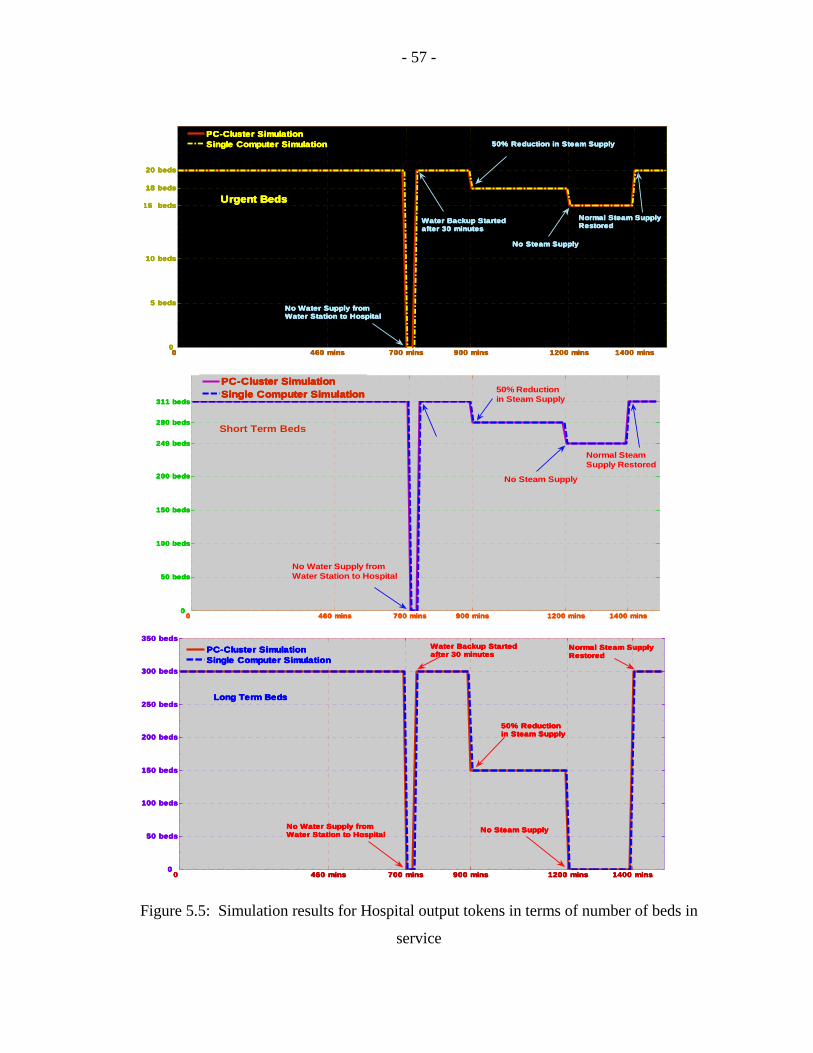
- 57 -

0 0 0 0 460 mins460 mins460 mins460 mins 700 mins700 mins700 mins700 mins 900 mins900 mins900 mins900 mins 1200 mins1200 mins1200 mins1200 mins 1400 mins1400 mins1400 mins1400 mins0 0 0 0

5 beds5 beds5 beds5 beds

10 beds 10 beds 10 beds 10 beds

16 beds16 beds16 beds16 beds

18 beds18 beds18 beds18 beds

20 beds20 beds20 beds20 beds

PC-Cluster SimulationPC-Cluster SimulationPC-Cluster SimulationPC-Cluster SimulationSingle Computer SimulationSingle Computer SimulationSingle Computer SimulationSingle Computer Simulation

Urgent BedsUrgent BedsUrgent BedsUrgent Beds

No Water Supply fromNo Water Supply fromNo Water Supply fromNo Water Supply fromWater Station to HospitalWater Station to HospitalWater Station to HospitalWater Station to Hospital

Water Backup StartedWater Backup StartedWater Backup StartedWater Backup Startedafter 30 minutesafter 30 minutesafter 30 minutesafter 30 minutes

50% Reduction in Steam Supply50% Reduction in Steam Supply50% Reduction in Steam Supply50% Reduction in Steam Supply

No Steam SupplyNo Steam SupplyNo Steam SupplyNo Steam Supply

Normal Steam SupplyNormal Steam SupplyNormal Steam SupplyNormal Steam SupplyRestoredRestoredRestoredRestored

0 0 0 0 460 mins460 mins460 mins460 mins 700 mins700 mins700 mins700 mins 900 mins900 mins900 mins900 mins 1200 mins1200 mins1200 mins1200 mins 1400 mins1400 mins1400 mins1400 mins0 0 0 0

50 beds50 beds50 beds50 beds

100 beds100 beds100 beds100 beds

150 beds150 beds150 beds150 beds

200 beds200 beds200 beds200 beds

249 beds249 beds249 beds249 beds

280 beds280 beds280 beds280 beds

311 beds311 beds311 beds311 beds

PC-Cluster SimulationPC-Cluster SimulationPC-Cluster SimulationPC-Cluster SimulationSingle Computer SimulationSingle Computer SimulationSingle Computer SimulationSingle Computer Simulation

No Water Supply fromWater Station to Hospital

50% Reductionin Steam Supply

No Steam Supply

Normal SteamSupply Restored

Short Term Beds

0 0 0 0 460 mins460 mins460 mins460 mins 700 mins700 mins700 mins700 mins 900 mins900 mins900 mins900 mins 1200 mins1200 mins1200 mins1200 mins 1400 mins1400 mins1400 mins1400 mins0 0 0 0

50 beds50 beds50 beds50 beds

100 beds100 beds100 beds100 beds

150 beds150 beds150 beds150 beds

200 beds200 beds200 beds200 beds

250 beds250 beds250 beds250 beds

300 beds300 beds300 beds300 beds

350 beds350 beds350 beds350 beds

PC-Cluster SimulationPC-Cluster SimulationPC-Cluster SimulationPC-Cluster SimulationSingle Computer SimulationSingle Computer SimulationSingle Computer SimulationSingle Computer Simulation

No Water Supply fromNo Water Supply fromNo Water Supply fromNo Water Supply fromWater Station to HospitalWater Station to HospitalWater Station to HospitalWater Station to Hospital

Water Backup StartedWater Backup StartedWater Backup StartedWater Backup Startedafter 30 minutesafter 30 minutesafter 30 minutesafter 30 minutes

50% Reduction50% Reduction50% Reduction50% Reductionin Steam Supplyin Steam Supplyin Steam Supplyin Steam Supply

No Steam SupplyNo Steam SupplyNo Steam SupplyNo Steam Supply

Normal Steam SupplyNormal Steam SupplyNormal Steam SupplyNormal Steam SupplyRestoredRestoredRestoredRestored

Long Term BedsLong Term BedsLong Term BedsLong Term Beds

Figure 5.5: Simulation results for Hospital output tokens in terms of number of beds in

service

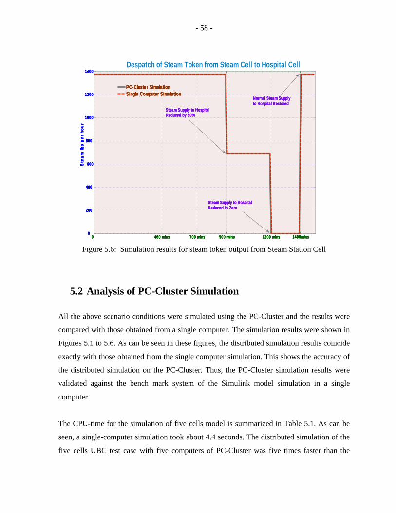
- 58 -

0 0 0 0 460 mins460 mins460 mins460 mins 700 mins700 mins700 mins700 mins 900 mins900 mins900 mins900 mins 1200 mins1200 mins1200 mins1200 mins 1400mins1400mins1400mins1400mins0 0 0 0

200 200 200 200

400 400 400 400

600600600600

800 800 800 800

1000100010001000

1200120012001200

1400140014001400

Ste

am

lb

s p

er

ho

ur

Ste

am

lb

s p

er

ho

ur

Ste

am

lb

s p

er

ho

ur

Ste

am

lb

s p

er

ho

ur

PC-Cluster SimulationPC-Cluster SimulationPC-Cluster SimulationPC-Cluster SimulationSingle Computer SimulationSingle Computer SimulationSingle Computer SimulationSingle Computer Simulation

Steam Supply to HospitalSteam Supply to HospitalSteam Supply to HospitalSteam Supply to HospitalReduced by 50%Reduced by 50%Reduced by 50%Reduced by 50%

Steam Supply to HospitalSteam Supply to HospitalSteam Supply to HospitalSteam Supply to HospitalReduced to ZeroReduced to ZeroReduced to ZeroReduced to Zero

Normal Steam SupplyNormal Steam SupplyNormal Steam SupplyNormal Steam Supplyto Hospital Restoredto Hospital Restoredto Hospital Restoredto Hospital Restored

Despatch of Steam Token from Steam Cell to Hospital Cell

Figure 5.6: Simulation results for steam token output from Steam Station Cell

5.2 Analysis of PC-Cluster Simulation

All the above scenario conditions were simulated using the PC-Cluster and the results were

compared with those obtained from a single computer. The simulation results were shown in

Figures 5.1 to 5.6. As can be seen in these figures, the distributed simulation results coincide

exactly with those obtained from the single computer simulation. This shows the accuracy of

the distributed simulation on the PC-Cluster. Thus, the PC-Cluster simulation results were

validated against the bench mark system of the Simulink model simulation in a single

computer.

The CPU-time for the simulation of five cells model is summarized in Table 5.1. As can be

seen, a single-computer simulation took about 4.4 seconds. The distributed simulation of the

five cells UBC test case with five computers of PC-Cluster was five times faster than the

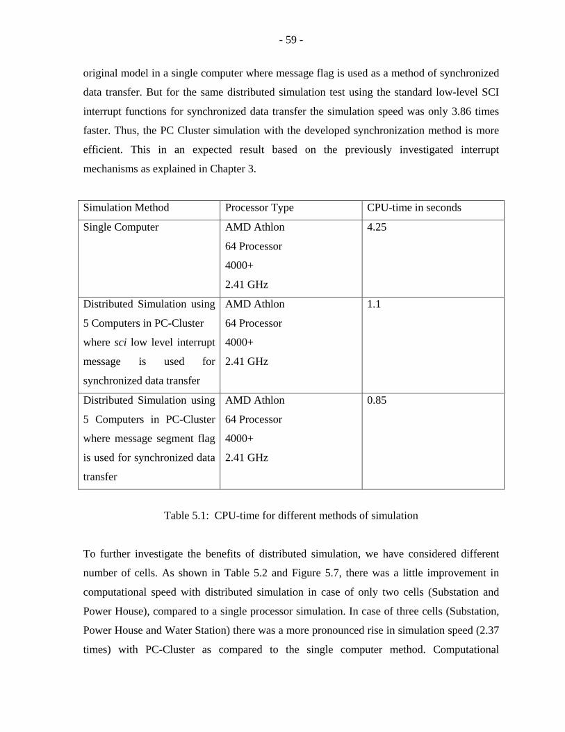
- 59 -

original model in a single computer where message flag is used as a method of synchronized

data transfer. But for the same distributed simulation test using the standard low-level SCI

interrupt functions for synchronized data transfer the simulation speed was only 3.86 times

faster. Thus, the PC Cluster simulation with the developed synchronization method is more

efficient. This in an expected result based on the previously investigated interrupt

mechanisms as explained in Chapter 3.

Simulation Method Processor Type CPU-time in seconds

Single Computer AMD Athlon

64 Processor

4000+

2.41 GHz

4.25

Distributed Simulation using

5 Computers in PC-Cluster

where sci low level interrupt

message is used for

synchronized data transfer

AMD Athlon

64 Processor

4000+

2.41 GHz

1.1

Distributed Simulation using

5 Computers in PC-Cluster

where message segment flag

is used for synchronized data

transfer

AMD Athlon

64 Processor

4000+

2.41 GHz

0.85

Table 5.1: CPU-time for different methods of simulation

To further investigate the benefits of distributed simulation, we have considered different

number of cells. As shown in Table 5.2 and Figure 5.7, there was a little improvement in

computational speed with distributed simulation in case of only two cells (Substation and

Power House), compared to a single processor simulation. In case of three cells (Substation,

Power House and Water Station) there was a more pronounced rise in simulation speed (2.37

times) with PC-Cluster as compared to the single computer method. Computational

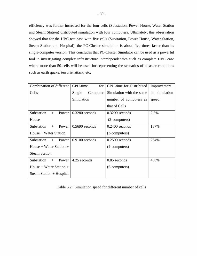
- 60 -

efficiency was further increased for the four cells (Substation, Power House, Water Station

and Steam Station) distributed simulation with four computers. Ultimately, this observation

showed that for the UBC test case with five cells (Substation, Power House, Water Station,

Steam Station and Hospital), the PC-Cluster simulation is about five times faster than its

single-computer version. This concludes that PC-Cluster Simulator can be used as a powerful

tool in investigating complex infrastructure interdependencies such as complete UBC case

where more than 50 cells will be used for representing the scenarios of disaster conditions

such as earth quake, terrorist attack, etc.

Combination of different

Cells

CPU-time for

Single Computer

Simulation

CPU-time for Distributed

Simulation with the same

number of computers as

that of Cells

Improvement

in simulation

speed

Substation + Power

House

0.3280 seconds 0.3200 seconds

(2-computers)

2.5%

Substation + Power

House + Water Station

0.5690 seconds 0.2400 seconds

(3-computers)

137%

Substation + Power

House + Water Station +

Steam Station

0.9100 seconds 0.2500 seconds

(4-computers)

264%

Substation + Power

House + Water Station +

Steam Station + Hospital

4.25 seconds 0.85 seconds

(5-computers)

400%

Table 5.2: Simulation speed for different number of cells

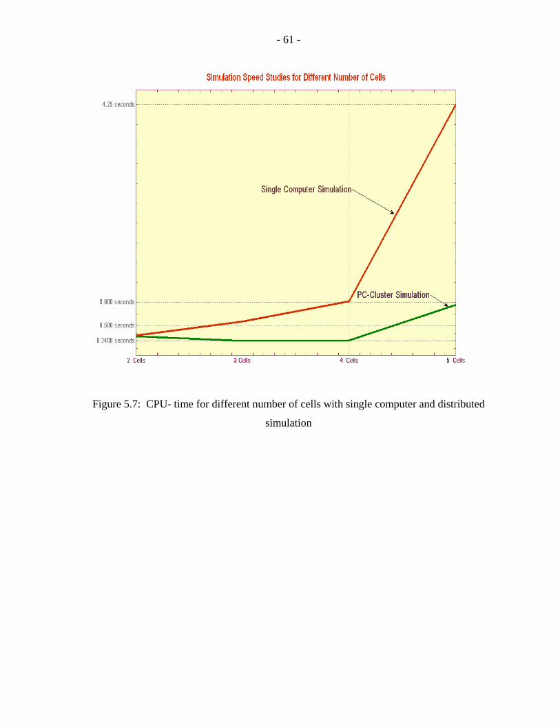
- 61 -

Figure 5.7: CPU- time for different number of cells with single computer and distributed

simulation

- 62 -

Chapter 6

Conclusions and future work In this thesis, a SCI-based PC-Cluster simulator for studying the interdependent nature of

critical infrastructures was developed where the computational superiority of a clustered

multi processor PC-Cluster over a sequential single processor system was demonstrated. A

practical scaled test case of the University of British Columbia (UBC) campus was used. The

UBC model included a substation, hospital, water station, power house and steam station.

The test model was distributed among five computers of the PC-Cluster. The PC-Cluster

used in this research consists of 16 computers networked via high speed SCI interconnect

adapter cards. A set of C-language based communication libraries based on optimum SCI

low-level functions was developed, in order to use the hardware interconnect efficiently.

Furthermore, a Simulink S-function block using these communication functions was built for

parallel simulation of Simulink models distributed in different computers of the PC-Cluster.

With the implementation of SCI low-level interrupt function for synchronized back and forth

zero-length data transfer between nodes, the measured communication overhead was

40µseconds. In case of message polling method of bi-directional synchronized zero-length

data transfer the communication latency was 7.2µseconds.

The PC-Cluster based distributed simulation plot results for the UBC test case were identical

as those obtained from sequential simulation on a single computer. The message polling

synchronized data transfer based distributed simulation on PC-Cluster was nearly five times

faster than the simulation of the original model on a single computer. On the other hand, SCI

low-level interrupt function synchronized data transfer method of distributed simulation is

3.86 times faster than that obtained on a single processor. There is a negligible improvement

in PC-Cluster simulation speed compared to a single node simulation in case of models with

less complexity such as two cells: substation and power house. When the number of cells

- 63 -

increases to five, the distributed parallel computing showed a remarkable improvement in

computation speed compared to that of one processor simulation. Hence PC-Cluster

simulator is proposed for better computational efficiency and feasibility of investigating the

interdependencies of complex and critical infrastructures.

Future research would include the implementation of the OVNI (Object Virtual Network

Integrator) method and I2SIM (Infrastructure Interdependencies Simulator) on SCI-based

PC-Cluster using the MATE (“Multi-Area Thévénin Equivalent”) network partitioning

technique [1], [2], [3]. Here one master node contains a memory segment to which all other

sub-systems residing on other nodes will send Thévénin Equivalent data. Then the master

node solves the reduced system represented by the links subsystem. The updated link

currents are then communicated back to the sub-systems and the whole process starts again.

For this, a method of sending data from different nodes to a single node with a common

memory segment should be developed [3] on SCI. Additionally, this distributed PC-Cluster

simulation with different t’s (simulation time step) should be investigated in order to

achieve better computational efficiency due to less communication overhead.

- 64 -

References

Chapter 1 [1] Mansell, Rankin and Associates, "Joint Infrastructure Interdependencies Research Program (JIIRP) Symposium," 198 Holmwood Avenue, Ottawa, ON, Canada, November 10, 2005. [2] J. A. Hollman, J. R. Marti, J. Jatskevich and K. Srivastava, "Dynamic islanding of critical infrastructures: a suitable strategy to survive and mitigate extreme events," International Journal of Emergency Management, vol. 4, pp. 45-58, 2007. [3] D. D. Dudenhoeffer, M. R. Permann and E. M. Sussman, "General methodology 3: a parallel simulation framework for infrastructure modeling and analysis," Proceedings of the 34th Conference on Winter Simulation: Exploring New Frontiers, pp. 1971-1977, 2002. [4] W. Gropp and E. Lusk, "User’s Guide for mpich, a Portable Implementation of MPI Version 1.2. 1," Argonne National Laboratory, USA 1996.

[5] IEEE Standard for Scalable Coherent Interface (SCI), IEEE Std 1596-1992, March 1992. [6] S. Garg and J. Mache, "Performance evaluation of parallel file systems for PC clusters and ASCI red," Cluster Computing, 2001.Proceedings.2001 IEEE International Conference on, pp. 172-177, 2001. [7] "PCI-SCI Adapter Card D320/321 Functional Overview," Dolphin Interconnect Solutions Inc., Version 1.01, Oslo, Norway, November 30, 1999. [Online]. Available: http://www.dolphinics.com

[8] "Low-level SCI software functional specification," Dolphin Interconnect Solutions Inc., Oslo, Norway, Espirit Project 23174 – Software Infrastructure for SCI (SISCI), Version 2.1.1 – March 15, 1999. [Online]. Available: http://www.dolphinics.com

[9] "SIMULINK: Dynamic System Simulation for MATLAB," Using Simulink Version 7, The Math Works Inc., 2003.

- 65 -

Chapter 2 [1] IEEE Standard for Scalable Coherent Interface (SCI), IEEE Std 1596-1992, March 1992. [2] N. Boden, D. Cohen, R. Felderman, A. Kulawik, C. Seitz and J. Seizovic, "Myrinet: a gigabit-per-second local area network," Micro, IEEE, vol. 15, pp. 29-36, 1995. [3] C. Dubnicki, A. Bilas, Y. Chen, S. N. Damianakis and K. Li, "Shrimp Project Update: Myrinet Communication," IEEE Micro, vol. 18, pp. 50-52, 1998. [4] S. H. Chung, S. C. Oh, S. Park and H. Jang, "Utilizing network cache on an SCI-based PC cluster," Parallel and Distributed Processing Symposium., Proceedings 15th International, pp. 1666-1672, 2001. [5] "SCRAMNet+ Shared Memory- Speed, Determinism, Reliability, and Flexibility For Distributed Real-Time Systems," Curtiss-Wright Controls Embedded Computing, Dayton, Ohio, USA, 2004. [6] "M3S-PCI64B and M3S-PCI64C, Universal, 64/32-bit, 66/33MHz, Myrinet-2000-Serial- Link/PCI interfaces," Guide to Myrinet-2000 Switches and Switch Networks, 2001. Myricom Inc.. [7] "SCRAMNet+ SC150 Network PCI bus hardware reference," Document No. D-T- MR-PCI-A-0-A7, Systran Corporation , Dayton , Ohio, USA, November 10, 2000. [8] "Dolphin Interconnect Solutions Inc. – Benchmarks," Dolphin Interconnect Solutions Inc., Oslo, Norway, 2006. [Online]. Available: http://www.dolphinics.com/products/benchmarks.html. [9] "Dolphin Interconnect Solutions Inc. – D350 Series PCI Express," Dolphin Interconnect Solutions Inc., Oslo, Norway, 2006. [Online]. Available: http://www.dolphinics.com/products/hardware/d350.html

[10] "PCI-SCI Adapter Card for System Area Networks," Dolphin Interconnect Solutions Inc. ., Oslo, Norway, 2006. [Online]. Available: http://www.dolphinics.com. [11] "SCIzzl: the Local Area Memory Port, Local Area Multiprocessor, Scalable Coherent Interface and Serial Express Users, Developers, and Manufacturers Association,". [Online]. Available: http://www.SCIzzl.com [12] H. Hellwagner and A. Reinefeld, SCI-Scalable Coherent Interface: Scalable Coherent Interface: Architecture and Software for High-Performance Compute Clusters. Springer, 1999.

- 66 -

[13] D. Gustavson and Q. Li, "The Scalable Coherent Interface (SCI)," Communications Magazine, IEEE, vol. 34, pp. 52-63, 1996. [14] "Link Controller LC-2 Specification. Data Sheet," Dolphin Interconnect Solutions Inc., Oslo, Norway, 1997. [Online]. Available: http://www.dolphinics.com [15] "Installation Guide for the Dolphin Adapter Card," Dolphin Interconnect Solutions Inc., Oslo, Norway, February 2003. [Online] Available: http://www.dolphinics.com

Chapter 3 [1] "Low-level SCI software functional specification," Dolphin Interconnect Solutions Inc., Oslo, Norway, Espirit Project 23174 – Software Infrastructure for SCI (SISCI), Version 2.1.1 – March 15, 1999. [Online]. Available: http://www.dolphinics.com [2] "SIMULINK: Dynamic System Simulation for MATLAB, " Using Simulink Version 7, The Math Works Inc., 2003. [3] H. Hellwagner and A. Reinefeld, SCI-Scalable Coherent Interface: Scalable Coherent Interface: Architecture and Software for High-Performance Compute Clusters. Springer, 1999. [4] T. A. Ngo and L. Snyder, "Data Locality on Shared Memory Computers Under Two Programming Models" Technical Report 93-06-08, Dept. Of CS, and IBM Research Report R19082, Univ. of Washington 1993. [5] "PSB32/64 Functional Specification," Dolphin Interconnect Solutions Inc., Oslo, Norway, February 2003. [Online]. Available: http://www.dolphinics.com [6] R. Hauser, "An Implementation of the SCI PHY-API (IEEEStd P1596. 9 Draft 0.41) for Dolphin PCI-SCI Boards," CERN Internal Note.Draft, vol. 1, 1997.

[7] "SISCI, Standard Software Infrastructures for SCI-based Parallel Systems," Dolphin Interconnect Solutions Inc., Oslo, Norway, Espirit Project 23174 – Software Infrastructure for SCI (SISCI), 1997. [8] F. Giacomini, T. Amundsen, A. Bogaerts, R. Hauser, B. Johnsen, H. Kohmann, R. Nordstrøm and P. Werner, "Low-level SCI software functional specification," Esprit Project, vol. 23174, 1999. [9] "Low-level SCI software requirements, analysis and pre-design," Dolphin Interconnect Solutions Inc., Oslo, Norway, Espirit Project 23174 – Software Infrastructure for SCI (SISCI), Deliverable D.1.1.1 Version 2.0 – May , 1998. [Online]. Available: http//: www.dolphinics.com

- 67 -

[10] American National Standard Institute, Rationale for the ANSI C Programming Language, Silicon. Press, Summit, NJ, USA, 1990. [11] E. E. L. Mitchell and J. S. Gauthier, ACSL: Advanced Continuous Simulation Language–User Guide/Reference Manual, 1991. [12] Microtran Power System Analysis Corporation, "Reference Manual, Transients Analysis Program for Power and Power Electronic Circuits," Vancouver, Canada, 2002. [13] Distributed Simulation Toolbox, Distributed and parallel simulation within Simulink or Stateflow, The Math Works – Third-Party Products & Services, The Math Works Inc., 2003. [Online]. Avalable: http://www.mathworks.com/products/connections/product_main.html [14] EXTESSY Inter Tool Exchange (EXITE), EXTESSY AG, Major-Hirst-Str. 11 38442 Wolfsburg, Germany. [Online]. Available: http://www.extessy.com

Chapter 4 [1] Lu Liu, "Prototyping and Cells Modeling of the Infrastructure Interdependencies Simulator I2SIM," M.A.Sc. thesis, to be submitted, Dept. of Electrical and Computer Engineering, The University of British Columbia, Vancouver, Canada, August 2007. [2] J. Hollman, D. Grigg, "Campus Case: Experiences from a collaborative effort, " JIIRP Industry Symposium, Vancouver, Canada, February 26, 2007. [3] J. Martí, J. Hollman, C. Ventura and J. Jatskevich, "Design for Survival Real-time Infrastructures Coordination," in Proceedings of the International Workshop on Complex Network and Infrastructure Protection (CNIP), Rome, Italy, 2006. [4] J. A. Hollman, J. R. Marti, J. Jatskevich and K. Srivastava, "Dynamic islanding of critical infrastructures: a suitable strategy to survive and mitigate extreme events," International Journal of Emergency Management, vol. 4, pp. 45-58, 2007. [5] P. Kruchten, C. Woo, "Modeling Disasters," JIIRP Seminar presentation, Vancouver, Canada, September 2005 . [6] J. Martí, J. Hollman, C. Ventura, J. Jatskevich, "Transportation Matrix Model for Infrastructures Disaster Coordination," JIIRP Seminar presentation, Vancouver, Canada, February 2006.

[7] A.C. Chiang, Fundamental Methods of Mathematical Economics, Third Ed., McGraw- Hill, 1984. [8] A.P. Sage, Methodology for Large-Scale Systems, McGraw-Hill, 1977.

- 68 -

[9] J.R.Martí, L. Liu, "UBC Campus Case: Cell Modeling EE Computer Society, " Internal report, The University of British Columbia,Vancouver, Canada, August 2006

Chapter 5 [1] Lu Liu, "Prototyping and Cells Modeling of the Infrastructure Interdependencies Simulator I2SIM," M.A.Sc. thesis, to be submitted, Dept. of Electrical and Computer Engineering, The University of British Columbia, Vancouver, Canada, August 2007.

Chapter 6 [1] J.R. Martí, L.R. Linares, J. Calviño, H.W. Dommel, and J. Lin, "OVNI: Integrated software/hardware solution for real-time simulation of large power systems," in 14th Power Systems Computation Conference, Sevilla, Spain, 2002, PSCC’02.

[2] J.R. Martí, L.R. Linares, J. Calviño, and H.W. Dommel, "OVNI: An Object Approach to Real-Time Power System Simulators," in Proceedings of the 1998 International Conference on Power System Technology, Powercon’98, Beijing, China, August 18-21, 1998. [3] T.D. Rybel, J. A. Hollman, J.R. Martí, " OVNI-NET: A flexible cluster interconnect for the new OVNI Real-Time simulator," in 15th Power Systems Computation Conference, Liege, Belgium, 2005, PSCC’05.

- 69 -

Appendix Computer Programs /* ----------------------------------------------------------------------------------------------------------------------------*/ /* */ /* FILE NAME : COMPUTER1.C */ /* DESCRIPTION : Measurement of Communication Latency between two * /* Computers using two different methods of synchronous */ /* back and forth data transfer */ /* */ /* ----------------------------------------------------------------------------------------------------------------------------*/ #include <stdio.h> #include <string.h> #include <stdlib.h> #include <sci_comm_lib.h> void main () { int localNodeId = 4; /*computer 1 */ int remoteNodeId = 8; /*computer 2 */ int vecsize = 100; int h = 1; double y [100], x [100]; int i; scistart (&h);

sciinit (&h, localNodeId, remoteNodeId, vecsize);

for (i=0; i<vecsize-1; i++) { x [i] = (double) i; } scireceive (&h, y, vecsize); scisend (&h, x, vecsize);

sciend (&h);

sciclose (&h);

}

- 70 -

/* ----------------------------------------------------------------------------------------------------------------------------*/ /* */ /* FILE NAME : COMPUTER2.C */ /* DESCRIPTION : Measurement of Communication Latency between two * /* Computers using two different methods of synchronous */ /* back and forth data transfer */ /* */ /* ----------------------------------------------------------------------------------------------------------------------------*/ #include <stdio.h> #include <string.h> #include <stdlib.h> #include <sci_comm_lib.h> void main () { int localNodeId = 8; /*computer 2 */ int remoteNodeId = 4; /*computer 1 */ int vecsize = 100; int h = 1; double y [100], x [100]; int i; scistart (&h);

sciinit (&h, localNodeId, remoteNodeId, vecsize);

for (i=0; i<vecsize-1; i++) { x [i] = (double) i; } scireceive (&h, y, vecsize); scisend (&h, x, vecsize);

sciend (&h);

sciclose (&h);

}

- 71 -

/*---------------------------------------------------------------------------------------------------------------------------*/ /* */ /* FILE NAME : COMMUNICATION_S_FUNCTION */ /* DESCRIPTION : This is the C-code for building Simulink S-function */ /* in order to facilitate communication between distributed */ /* Simulink models in different computers of the PC-Cluster */ /* */ /*---------------------------------------------------------------------------------------------------------------------------*/ #define S_FUNCTION_NAME SCI_COMM_LIB #define S_FUNCTION_LEVEL 2 #define NUM_INPUTS 2 /* Input Port 0 */ #define IN_PORT_0_NAME u0 #define INPUT_0_WIDTH 3 #define INPUT_DIMS_0_COL 1 #define INPUT_0_DTYPE real_T #define INPUT_0_COMPLEX COMPLEX_NO #define IN_0_FRAME_BASED FRAME_NO #define IN_0_DIMS 1-D #define INPUT_0_FEEDTHROUGH 1 #define IN_0_ISSIGNED 0 #define IN_0_WORDLENGTH 8 #define IN_0_FIXPOINTSCALING 1 #define IN_0_FRACTIONLENGTH 9 #define IN_0_BIAS 0 #define IN_0_SLOPE 0.125 /* Input Port 1 */ #define IN_PORT_1_NAME u1 #define INPUT_1_WIDTH 1 #define INPUT_DIMS_1_COL 1 #define INPUT_1_DTYPE real_T #define INPUT_1_COMPLEX COMPLEX_NO #define IN_1_FRAME_BASED FRAME_NO #define IN_1_DIMS 1-D #define INPUT_1_FEEDTHROUGH 1 #define IN_1_ISSIGNED 0 #define IN_1_WORDLENGTH 8 #define IN_1_FIXPOINTSCALING 1 #define IN_1_FRACTIONLENGTH 9 #define IN_1_BIAS 0

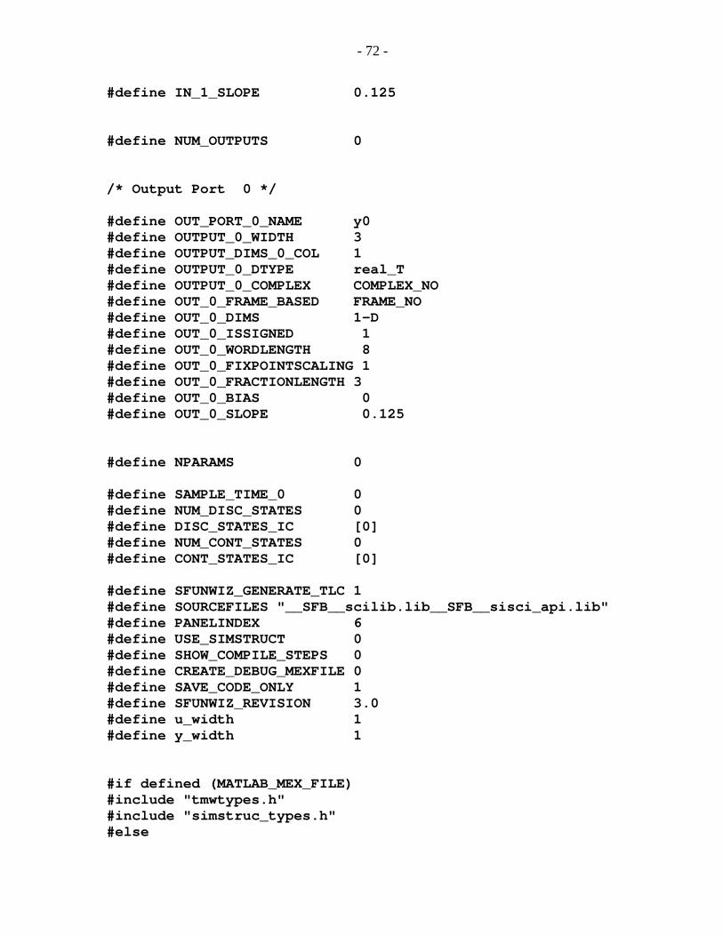
- 72 -

#define IN_1_SLOPE 0.125 #define NUM_OUTPUTS 0 /* Output Port 0 */ #define OUT_PORT_0_NAME y0 #define OUTPUT_0_WIDTH 3 #define OUTPUT_DIMS_0_COL 1 #define OUTPUT_0_DTYPE real_T #define OUTPUT_0_COMPLEX COMPLEX_NO #define OUT_0_FRAME_BASED FRAME_NO #define OUT_0_DIMS 1-D #define OUT_0_ISSIGNED 1 #define OUT_0_WORDLENGTH 8 #define OUT_0_FIXPOINTSCALING 1 #define OUT_0_FRACTIONLENGTH 3 #define OUT_0_BIAS 0 #define OUT_0_SLOPE 0.125 #define NPARAMS 0 #define SAMPLE_TIME_0 0 #define NUM_DISC_STATES 0 #define DISC_STATES_IC [0] #define NUM_CONT_STATES 0 #define CONT_STATES_IC [0] #define SFUNWIZ_GENERATE_TLC 1 #define SOURCEFILES "__SFB__scilib.lib__SFB__sisci_api.lib" #define PANELINDEX 6 #define USE_SIMSTRUCT 0 #define SHOW_COMPILE_STEPS 0 #define CREATE_DEBUG_MEXFILE 0 #define SAVE_CODE_ONLY 1 #define SFUNWIZ_REVISION 3.0 #define u_width 1 #define y_width 1 #if defined (MATLAB_MEX_FILE) #include "tmwtypes.h" #include "simstruc_types.h" #else

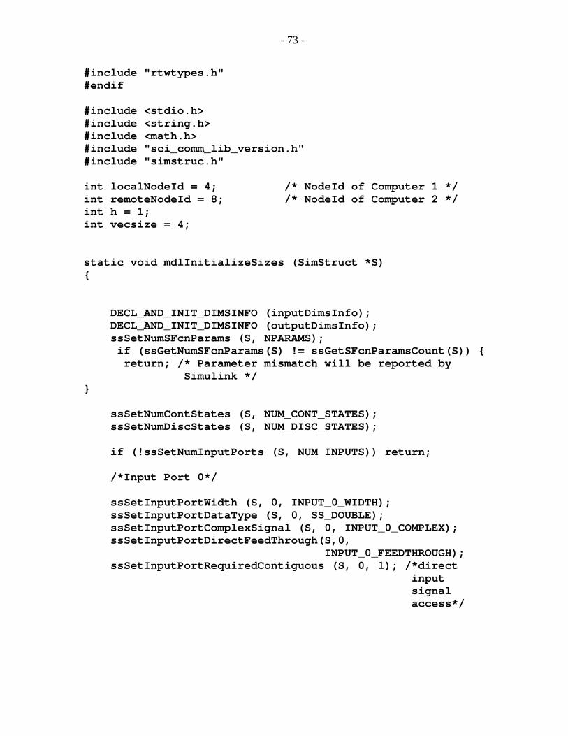
- 73 -

#include "rtwtypes.h" #endif #include <stdio.h> #include <string.h> #include <math.h> #include "sci_comm_lib_version.h" #include "simstruc.h" int localNodeId = 4; /* NodeId of Computer 1 */ int remoteNodeId = 8; /* NodeId of Computer 2 */ int h = 1; int vecsize = 4; static void mdlInitializeSizes (SimStruct *S) { DECL_AND_INIT_DIMSINFO (inputDimsInfo); DECL_AND_INIT_DIMSINFO (outputDimsInfo); ssSetNumSFcnParams (S, NPARAMS); if (ssGetNumSFcnParams(S) != ssGetSFcnParamsCount(S)) { return; /* Parameter mismatch will be reported by Simulink */ } ssSetNumContStates (S, NUM_CONT_STATES); ssSetNumDiscStates (S, NUM_DISC_STATES); if (!ssSetNumInputPorts (S, NUM_INPUTS)) return; /*Input Port 0*/ ssSetInputPortWidth (S, 0, INPUT_0_WIDTH); ssSetInputPortDataType (S, 0, SS_DOUBLE); ssSetInputPortComplexSignal (S, 0, INPUT_0_COMPLEX); ssSetInputPortDirectFeedThrough(S,0, INPUT_0_FEEDTHROUGH); ssSetInputPortRequiredContiguous (S, 0, 1); /*direct input signal access*/

- 74 -

/*Input Port 1*/ ssSetInputPortWidth (S, 1, INPUT_1_WIDTH); ssSetInputPortDataType (S, 1, SS_DOUBLE); ssSetInputPortComplexSignal (S, 1, INPUT_1_COMPLEX); ssSetInputPortDirectFeedThrough (S, 1, INPUT_1_FEEDTHROUGH); ssSetInputPortRequiredContiguous (S, 1, 1); /*direct input signal access*/ if (!ssSetNumOutputPorts (S, NUM_OUTPUTS)) return; /*Output Port 0*/ ssSetOutputPortWidth (S, 0, OUTPUT_0_WIDTH); ssSetOutputPortDataType (S, 0, SS_DOUBLE); ssSetOutputPortComplexSignal (S, 0, OUTPUT_0_COMPLEX); ssSetNumSampleTimes (S, 1); ssSetNumRWork (S, 0); ssSetNumIWork (S, 0); ssSetNumPWork (S, 0); ssSetNumModes (S, 0); ssSetNumNonsampledZCs (S, 0); ssSetOptions (S, (SS_OPTION_EXCEPTION_FREE_CODE | SS_OPTION_USE_TLC_WITH_ACCELERATOR | SS_OPTION_WORKS_WITH_CODE_REUSE)); } # define MDL_SET_INPUT_PORT_FRAME_DATA static void mdlSetInputPortFrameData (SimStruct *S, int_T port, Frame_T frameData) { ssSetInputPortFrameData (S, port, frameData); } static void mdlInitializeSampleTimes (SimStruct *S) { ssSetSampleTime (S, 0, SAMPLE_TIME_0);

- 75 -

ssSetOffsetTime (S, 0, 0.0); } #define MDL_SET_INPUT_PORT_DATA_TYPE static void mdlSetInputPortDataType (SimStruct *S, int port, DTypeId dType) { ssSetInputPortDataType ( S, 0, dType); ssSetInputPortDataType ( S, 1, dType); } #define MDL_SET_OUTPUT_PORT_DATA_TYPE static void mdlSetOutputPortDataType (SimStruct *S, int port, DTypeId dType) { ssSetOutputPortDataType (S, 0, dType); } #define MDL_SET_DEFAULT_PORT_DATA_TYPES static void mdlSetDefaultPortDataTypes (SimStruct *S) { ssSetInputPortDataType ( S, 0, SS_DOUBLE); ssSetInputPortDataType( S, 1, SS_DOUBLE); ssSetOutputPortDataType(S, 0, SS_DOUBLE); } #define MDL_INITIALIZE_CONDITIONS #if defined (MDL_INITIALIZE_CONDITIONS) static void mdlInitializeConditions (SimStruct *S) { } #endif #define MDL_START #if defined (MDL_START) static void mdlStart (SimStruct *S) { /*SCI functions to start and initialize the SCI environment */ scistart (&h); sciinit (&h, localNodeId, remoteNodeId, vecsize);

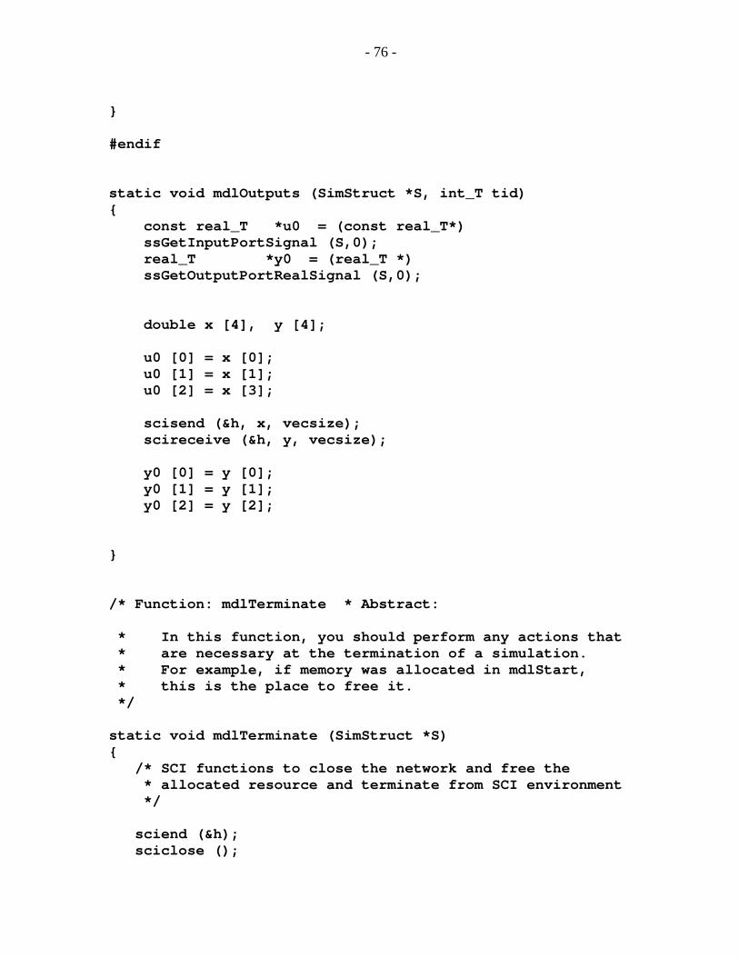
- 76 -

} #endif static void mdlOutputs (SimStruct *S, int_T tid) { const real_T *u0 = (const real_T*) ssGetInputPortSignal (S,0); real_T *y0 = (real_T *) ssGetOutputPortRealSignal (S,0); double x [4], y [4]; u0 [0] = x [0]; u0 [1] = x [1]; u0 [2] = x [3]; scisend (&h, x, vecsize); scireceive (&h, y, vecsize); y0 [0] = y [0]; y0 [1] = y [1]; y0 [2] = y [2]; } /* Function: mdlTerminate * Abstract: * In this function, you should perform any actions that * are necessary at the termination of a simulation. * For example, if memory was allocated in mdlStart, * this is the place to free it. */ static void mdlTerminate (SimStruct *S) { /* SCI functions to close the network and free the * allocated resource and terminate from SCI environment */ sciend (&h); sciclose ();

- 77 -

} #ifdef MATLAB_MEX_FILE /* Is this file being compiled as a MEX-file? */ #include "simulink.c" /* MEX-file interface mechanism */ #endif