Motion of half-spin particles in the axially symmetric field of naked

singularities of static q-metric

V.P.Neznamov1,2*, V.E.Shemarulin1†

1RFNC-VNIIEF, Russia, Sarov, Mira pr., 37, 607188

2National Research Nuclear University MEPhI, Moscow, Russia

Abstract

Quantum-mechanical motion of a half-spin particle was examined in the axially

symmetric field of static naked singularities formed by mass distribution with quadrupole

moment (q-metric). The analysis was performed by means of the method of effective potentials

of the Dirac equation generalized for the case when radial and angular variables are not

separated. As lim lim1 , 1q q q the naked singularities do not except the existence of

stationary bound states of Dirac particles for a prolate mass distribution in the q-metric along the

axial axis.

For the oblate mass distribution, the naked singularities of the q-metric are separated

from the Dirac particle by infinitely large repulsive barriers with the subsequent potential well

deepening while moving along the angle from the equator (or from min , min )

towards poles. The exception are the poles and, as *0 q q , some points i for the states of the

particle with 32j .

Key words: naked singularity, static q-metric, Dirac Hamiltonian, effective repulsive and

attraction potentials, cosmic censorship.

                                                            * E-mail: neznamov@vniief.ru † E-mail: shemarulin@vniief.ru

2

Introduction

In terms of multipole moments, the simplest static solution to Einstein vacuum equations

is the Schwarzschild metrics with a mass monopole moment only. The first vacuum solution

with the quadrupole mass moment was obtained by Weyl in 1917 [1]. Ever since, many papers

devoted to study of vacuum solutions with non-zero multipole moments have appeared in

literature (see, for instance, [2] - [14]). Rather a simple compact form for the quadrupole metric

(q-metric) was obtained in [4]. In spherical coordinates, it can be represented as

2

1 2 2 22 2 2 2 2 2 2 20 0 0

2 00

sin1 1 1 sin .

14 1

q q

q qr r r dr

ds c dt r d r drrr r rrr

(1)

In (1), 0 2

2GMr

c is the event horizon (the gravitational radius) of the Schwarzschild field.

Below, we are going to use the system of units 1c .

The q-metric is the axial-symmetric vacuum solution which as 0q is reduced to the

spherical-symmetric Schwarzschild metric.

From the positivity condition of the Arnowitt-Deser-Misner mass, the condition 1q

follows [13]. The interval 1,0q describes prolate mass distribution of the q-metric source

along the axial axis; the interval 0,q describes the oblate mass distribution.

The q-metric has naked singularities as 0r and 0r r . At some parameter values there

exists the third singularity [13], determined by the equation

2

2 200 sin 0.

4

rr r r (2)

Our paper is devoted to the study of quantum-mechanical motion of half-spin particles in

the field of naked singularities of the q-metric (1).

The analysis was performed by means of effective potentials of the Dirac equation in the

q-metric field. For such an analysis, the self-conjugate Hamiltonian was derived and the method

of effective potentials was generalized for the case when radial and angular variables are not

separated. As a result, it was shown that as lim1 0q q the naked singularities do not

prevent the possibility of existence beyond its stationary bound states of Dirac particles for the

prolate mass distribution in the q-metric (lim

1q , the value limq depends on the parameters of

the q-metric (1)).

3

For the oblate mass distribution, the naked singularities of the q-metric are separated

from the Dirac particle by infinitely high repulsive barriers with the subsequent potential well

deepening while moving along the angle from the equator (or from min , min )

towards the poles.

The exception are the poles and, as *0 q q , some points i for the states of the

particle with 32j . (The calculations performed by means of the software package “Maple”

have shown that *1.4142 2 1.41424q . The detailed description of *q is given in 3.1).

The paper is organized as follows: In section 1, the self-conjugate Dirac Hamiltonian in

the q-metric field is derived. In section 2, for the case when radial and angular variables are not

separated the method for obtaining effective potentials of the Dirac equation was generalized. In

section 3, the obtained effective potential is examined depending on ,r and initial parameters

of the q-metric. In section 4, the compliance of the obtained results with the hypothesis of

cosmic censorship is discussed. In Conclusions, the obtained results are briefly discussed.

1. Self-conjugate Hamiltonian of a half-spin particle in the q-metric

field

The required Hamiltonian is determined by means of algorithms for obtaining self-

conjugate Dirac Hamiltonians in the exterior gravitational fields by using the methods of pseudo-

Hermitian quantum mechanics [15] - [17].

In (1), let us denote

01 ,S

rf

r (3)

22 2

02

sin, 1 .

4

q q

S

ra r

r f

(4)

Then, the non-zero components of the metric tensor in (1) are

1 1 2 2 200 11 22 33; , ; , ; sin .q q q q

S S S Sg f g f a r g f a r r g f r (5)

The nonzero tetrad vectors in the Schwinger gauge [18] and the Dirac -matrix with the

global indices are

11 2 2 2

0 1 2 320 1 2 31 1

2 2; ; ; ,

sin, ,

q q qq

s s ss

f f fH f H H H

ra r a r r

(6)

4

11 2 2 2

0 0 1 1 2 2 3 321 1

2 2; ; ; .

sin, ,

q q qq

s s ss

f f ff

ra r ra r

(7)

In (6), (7), the underlined indices are local indices. The sign «~» over quantities means

that they are calculated using tetrads in Schwinger gauge.

For diagonal metric tensors g , the self-conjugate Hamiltonian in -representation

(with a plane scalar product of wave functions) is easily derived from the equality obtaining

in [17]

1,

2 red redH H H (8)

where

0 000 00

.kred k

m iH

g g x

(9)

In (8), the sign «+» means the Hermitian conjugation.

In (9), m is a mass of the Dirac particle, 00g is a component of inverse metric tensor.

Taking into account (5), (7), we obtain

1 1 1 210 0 1 0 1 0 22 2 2

1 1 12 2 2

1 2 1 20 2 0 32 2

12

1 1 1 1ctg

2 2

1 1 1.

2 sin

q q qqs

s s s

q q

s s

i fH f m if if

r r ra a ra

if if

r ra

(10)

The Dirac equation in the Hamiltonian form for a half-spin particle in the field of the

naked singularities of the q-metric has the form of

,

, .t

i H tt

r

r (11)

2. Effective potentials for the field of the naked singularities of

the q-metric

It is seen from the Hamiltonian (10) that the radial and angular variables ,r in the

equation (11) are not separated. The generalization of the standard method is needed to obtain

effective potentials by means of squaring Dirac equations for real radial wave functions.

Let us represent the wave function ,t r in (11) as

3

,, .

,

imiEtr

t e ei r

r (12)

5

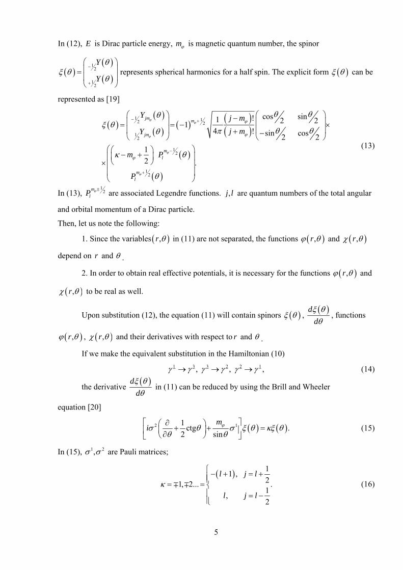
In (12), E is Dirac particle energy, m is magnetic quantum number, the spinor

1

2

12

Y

Y

represents spherical harmonics for a half spin. The explicit form can be

represented as [19]

1 12 2

12

12

12

cos sin!1 2 214 ! sin cos2 2

1

2 .

jmm

jm

m

l

m

l

Y j m

j mY

m P

P

(13)

In (13), 1

2m

lP are associated Legendre functions. ,j l are quantum numbers of the total angular

and orbital momentum of a Dirac particle.

Then, let us note the following:

1. Since the variables ,r in (11) are not separated, the functions ,r and ,r

depend on r and .

2. In order to obtain real effective potentials, it is necessary for the functions ,r and

,r to be real as well.

Upon substitution (12), the equation (11) will contain spinors , d

d

, functions

,r , ,r and their derivatives with respect to r and .

If we make the equivalent substitution in the Hamiltonian (10)

1 3 3 2 2 1, , , (14)

the derivative d

d

in (11) can be reduced by using the Brill and Wheeler

equation [20]

2 11ctg .

2 sin

mi

(15)

In (15), 1 2, are Pauli matrices;

1

1 ,21, 2... .1

,2

l j l

l j l

(16)

6

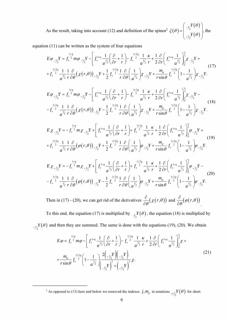
As the result, taking into account (12) and definition of the spinor‡

1

2

12

Y

Y

, the

equation (11) can be written as the system of four equations

1 1 21 12 2

1 1 11 1 12 2 22 2 2

1 2 1 2 1 2

2 2 21 1 11 1 1

2 2 22 2 2

1 1 1 1 1

2

1 1 1 1 1 1, 1 .

2 sin

q qq q

s s s s

q q q

s s s

E Y f m Y f f f Yr r r ra a a

mf r Y f Y f Y

r r ra a a

(17)

1 1 21 12 2

1 1 11 1 12 2 22 2 2

1 2 1 2 1 2

2 2 21 1 11 1 1

2 2 22 2 2

1 1 1 1 1

2

1 1 1 1 1 1, 1 .

2 sin

q qq q

s s s s

q q q

s s s

E Y f m Y f f f Yr r r ra a a

mf r Y f Y f Y

r r ra a a

(18)

1 1 21 12 2

1 1 11 1 12 2 22 2 2

1 2 1 2 1 2

2 2 21 1 11 1 1

2 2 22 2 2

1 1 1 1 1

2

1 1 1 1 1 1, 1 .

2 sin

q qq q

s s s s

q q q

s s s

E Y f m Y f f f Yr r r ra a a

mf r Y f Y f Y

r r ra a a

(19)

1 1 21 12 2

1 1 11 1 12 2 22 2 2

1 2 1 2 1 2

2 2 21 1 11 1 1

2 2 22 2 2

1 1 1 1 1

2

1 1 1 1 1 1, 1 .

2 sin

q qq q

s s s s

q q q

s s s

E Y f m Y f f f Yr r r ra a a

mf r Y f Y f Y

r r ra a a

(20)

Then in (17) - (20), we can get rid of the derivatives ,r

and ,r .

To this end, the equation (17) is multiplied by 12Y

, the equation (18) is multiplied by

12Y

and then they are summed. The same is done with the equations (19), (20). We obtain

1 1 21 12 2

1 1 12 2 2

1 2 1 12 22

1 2 22

1 12 2

1 1 1 1 1

2

211 .

sin

q qq q

s s s s

q

s

E f m f f fr r r ra a a

Y Ymf

r a Y Y

(21)

                                                            ‡ As opposed to (13) here and below we removed the indexes ,j m in notations 1

2Y

for short.

7

1 1 21 12 2

1 1 12 2 2

1 2 1 12 22

1 2 22

1 12 2

1 1 1 1 1

2

211 .

sin

q qq q

s s s s

q

s

E f m f f fr r r ra a a

Y Ymf

r a Y Y

(22)

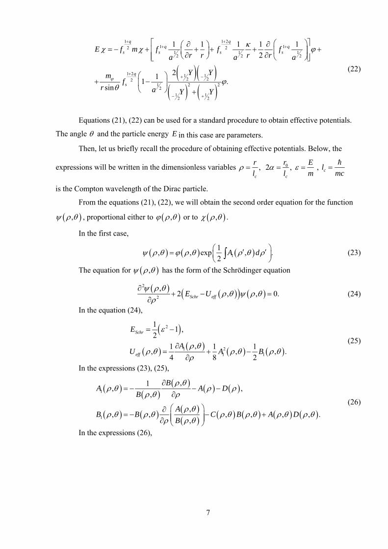
Equations (21), (22) can be used for a standard procedure to obtain effective potentials.

The angle and the particle energy E in this case are parameters.

Then, let us briefly recall the procedure of obtaining effective potentials. Below, the

expressions will be written in the dimensionless variables 0, 2 ,c c

r r E

l l m , cl mc

is the Compton wavelength of the Dirac particle.

From the equations (21), (22), we will obtain the second order equation for the function

, , proportional either to , or to , .

In the first case,

1

1, , exp , .

2A d

(23)

The equation for , has the form of the Schrödinger equation

2

2

,2 , , 0.Schr effE U

(24)

In the equation (24),

2

211 1

11 ,

2,1 1 1

, , , .4 8 2

Schr

eff

E

AU A B

(25)

In the expressions (23), (25),

1

1

,1, ,

,

,, , , , , , .

,

BA A D

B

AB B C B A D

B

(26)

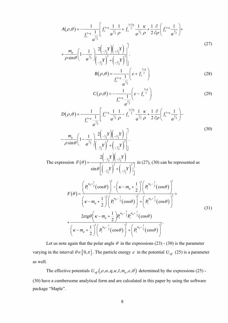
In the expressions (26),

8

1 21 12

1 1 12 2 21

12

1 12 2

1 2 22

1 12 2

1 1 1 1 1 1,

1 2

211 .

sin

qq q

s s sq

s

A f f fa a af

a

Y Ym

a Y Y

(27)

1

2

11

2

1, .

1

q

sq

s

B ff

a

(28)

1

2

11

2

1, .

1

q

sq

s

C ff

a

(29)

1 21 12

1 1 12 2 21

12

1 12 2

1 2 22

1 12 2

1 1 1 1 1 1,

1 2

211 .

sin

qq q

s s sq

s

D f f fa a af

a

Y Ym

a Y Y

(30)

The expression

1 12 2

2 2

1 12 2

2

sin

Y YF

Y Y

in (27), (30) can be represented as

2 221 1

2 2

2 22 1 1

2 2

1 1

2 2

2 22 1 1

2 2

1cos cos

2

1cos cos

2

12ctg cos

2 .1

cos cos2

m m

l l

m m

l l

m m

l l

m m

l l

P m P

F

m P P

m P P

m P P

(31)

Let us note again that the polar angle in the expressions (23) - (30) is the parameter

varying in the interval 0, . The particle energy in the potential effU (25) is a parameter

as well.

The effective potentials , , , , , , ,effU q l m determined by the expressions (25) -

(30) have a cumbersome analytical form and are calculated in this paper by using the software

package “Maple”.

9

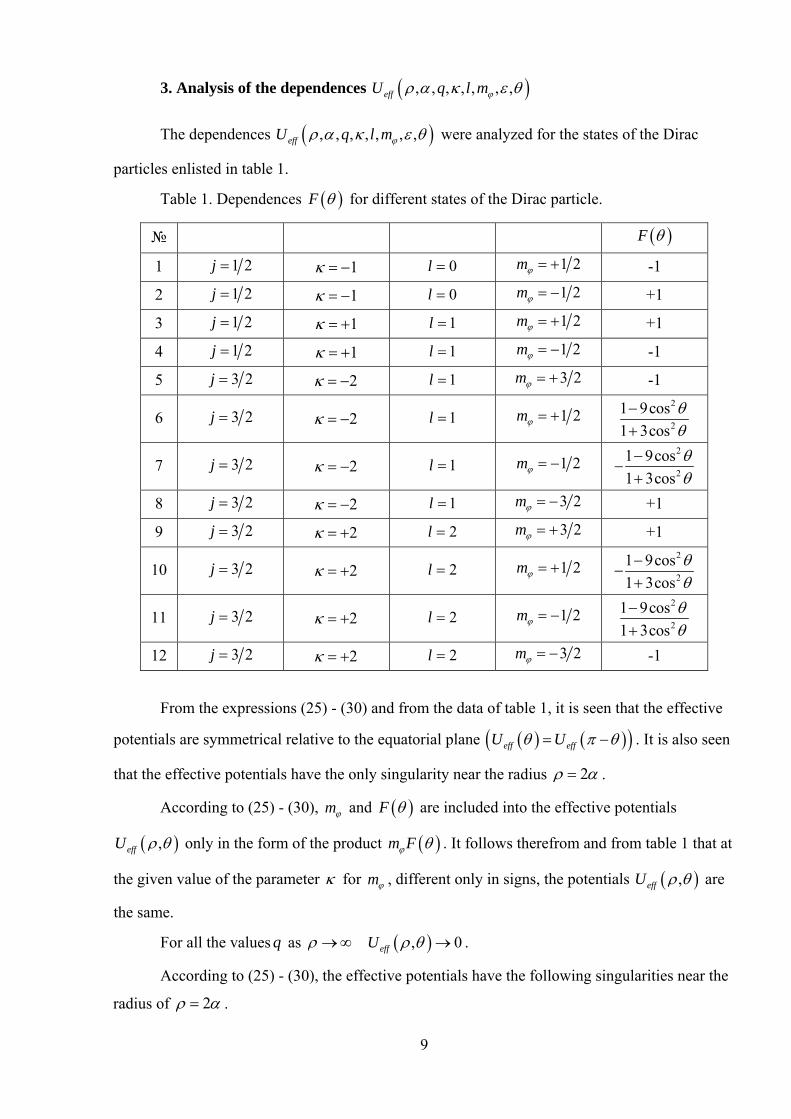
3. Analysis of the dependences , , , , , , ,effU q l m

The dependences , , , , , , ,effU q l m were analyzed for the states of the Dirac

particles enlisted in table 1.

Table 1. Dependences F for different states of the Dirac particle.

№ F

1 1 2j 1 0l 1 2m -1

2 1 2j 1 0l 1 2m +1

3 1 2j 1 1l 1 2m +1

4 1 2j 1 1l 1 2m -1

5 3 2j 2 1l 3 2m -1

6 3 2j 2 1l 1 2m 2

2

1 9cos

1 3cos

7 3 2j 2 1l 1 2m 2

2

1 9cos

1 3cos

8 3 2j 2 1l 3 2m +1

9 3 2j 2 2l 3 2m +1

10 3 2j 2 2l 1 2m 2

2

1 9cos

1 3cos

11 3 2j 2 2l 1 2m 2

2

1 9cos

1 3cos

12 3 2j 2 2l 3 2m -1

From the expressions (25) - (30) and from the data of table 1, it is seen that the effective

potentials are symmetrical relative to the equatorial plane eff effU U . It is also seen

that the effective potentials have the only singularity near the radius 2 .

According to (25) - (30), m and F are included into the effective potentials

,effU only in the form of the product m F . It follows therefrom and from table 1 that at

the given value of the parameter for m , different only in signs, the potentials ,effU are

the same.

For all the values q as , 0effU .

According to (25) - (30), the effective potentials have the following singularities near the

radius of 2 .

10

For 0,

2 1 2 22

2 12

2.

2

q q

eff q

mU F

(32)

For 0, , the potential 2effU

changes the sign and has the form of

2 12 1 2

2 12

2sin 0 .

2

qq

eff qU

(33)

Besides, there exists singularity

22,

2eff

N qU

(34)

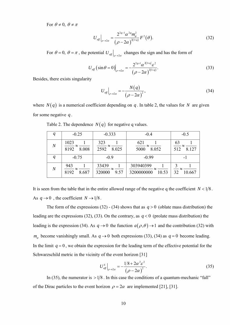
where N q is a numerical coefficient depending on q . In table 2, the values for N are given

for some negative q .

Table 2. The dependence N q for negative q values.

q -0.25 -0.333 -0.4 -0.5

N 1023 1

8192 8.008

323 1

2592 8.025

621 1

5000 8.052

63 1

512 8.127

q -0.75 -0.9 -0.99 -1

N 943 1

8192 8.687

33439 1

320000 9.57

303940399 1

3200000000 10.53

3 1

32 10.667

It is seen from the table that in the entire allowed range of the negative q the coefficient 1 8N .

As 0q , the coefficient 1 8N .

The form of the expressions (32) - (34) shows that as 0q (oblate mass distribution) the

leading are the expressions (32), (33). On the contrary, as 0q (prolate mass distribution) the

leading is the expression (34). As 0q the function , 1a and the contribution (32) with

m become vanishingly small. As 0q both expressions (33), (34) as 0q become leading.

In the limit 0q , we obtain the expression for the leading term of the effective potential for the

Schwarzschild metric in the vicinity of the event horizon [31]

2 2

22

1 8 2.

2SeffU

(35)

In (35), the numerator is 1 8 . In this case the conditions of a quantum-mechanic “fall”

of the Dirac particles to the event horizon 2 are implemented [21], [31].

11

3.1 Oblate mass distribution 0,q

For 0, , the leading term effU (25) has the form (32)

2 1 2 22

2 12

2.

2

q q

eff q

mU F

(36)

For 0, , the leading term effU changes the sign and has the form (33)

2 11 2 2

2 12

2sin 0 .

2

qq

eff qU

(37)

If 0F , the expression (36) represents an infinitely large repulsive barrier. The

barrier value sharply increases with the growth of q . On the contrary, as 0, the

leading term 2effU

represents a depth-unlimited potential well. At some values of , ,l m

and at certain values of i the function F and the expression (36) become equal to zero. In

table 1 0iF as

3 2, 2, 1 2, cos 1 3ij m ; 3 2, 2, 1 2, cos 1 3ij m .

In this case as i and * 2q q the leading term 2eff iU

, as before,

represents an infinitely high repulsive barrier of the following form

22

.2

eff i

LU

(38)

In (38), L is a coefficient increasing with the growth of q . As *q q , the repulsive

barrier disappears 0L . In the interval *0 q q , there appears a potential well of the

following form

122 2

eff i

LU

(39)

with the coefficient 1 1 8L .

Fig. 1 represents one-dimensional (with fixed values of the angle ) and two-

dimensional dependences ,effU for some states of a Dirac particle with positive values m

(Table 1, items 1, 3, 5, 6, 9, 10). The dependences ,effU for the states with the appropriate

negative values m do not quantitatively vary.

Let us discuss the form of ,effU in the interval 0, . For state 1 with 0l ,

the effective potential near the outer naked singularity 2 represents an infinitely large

12

repulsive barrier with a subsequent potential well. The finite depth of the well increases while

moving from the equator 2

towards the poles 0, .

For the states with 0l and 0F , the depth of the potential well is essentially

greater at positive . For certain states, the potential well disappears in the equatorial zone but

with the motion towards the poles it appears at certain values of min and min . The

finite depth of the well increases while moving along the angle towards the poles.

For states 6, 10 with 0l and 0iF as i and as *0 q q the positive

repulsive barrier disappears. Instead, an infinitely deep potential well (39) appears.

For all the examined cases at the poles 0, there exists an infinitely deep

potential well (37). Variations in q (fig. 2) and (fig. 3, 4) do not qualitatively change the

nature of the dependences ,effU .

3.2 Prolate mass distribution 1,0q

In this case, the leading term 2effU

has the form (34)

22,

2eff

N qU

(40)

Earlier, we have determined (see table 2) that for negative q the coefficient 1 8N . At

that, in the limit 0q , the coefficient 1 8N . However, at modulo small negative q ’s, an

essential contribution of the expression (33) is added to the expression (34). For 0q when

lim lim 1q q q , the function 2effU

approaches

2

1 1

8 2

. With the following

decrease in q , the potential effU tends to Schwarzschild limit (35). The value limq in

accordance with (33), (34) depends on the parameters of the q-metric (1) and the particle

energy . The numerical values limq can be determined by means of exact quantum-mechanical

calculations only.

In the interval lim 0q q , the condition of a quantum-mechanic “fall” of the Dirac

particle to the outer singularity 2 is implemented.

According to quantum mechanics, (see, for instance, [21]), the attractive singular

potential (40) for a prolate mass distribution as lim1 q q enables the possibility of existence

of stationary bound states of quantum-mechanical particles.

13

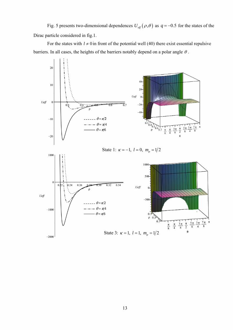
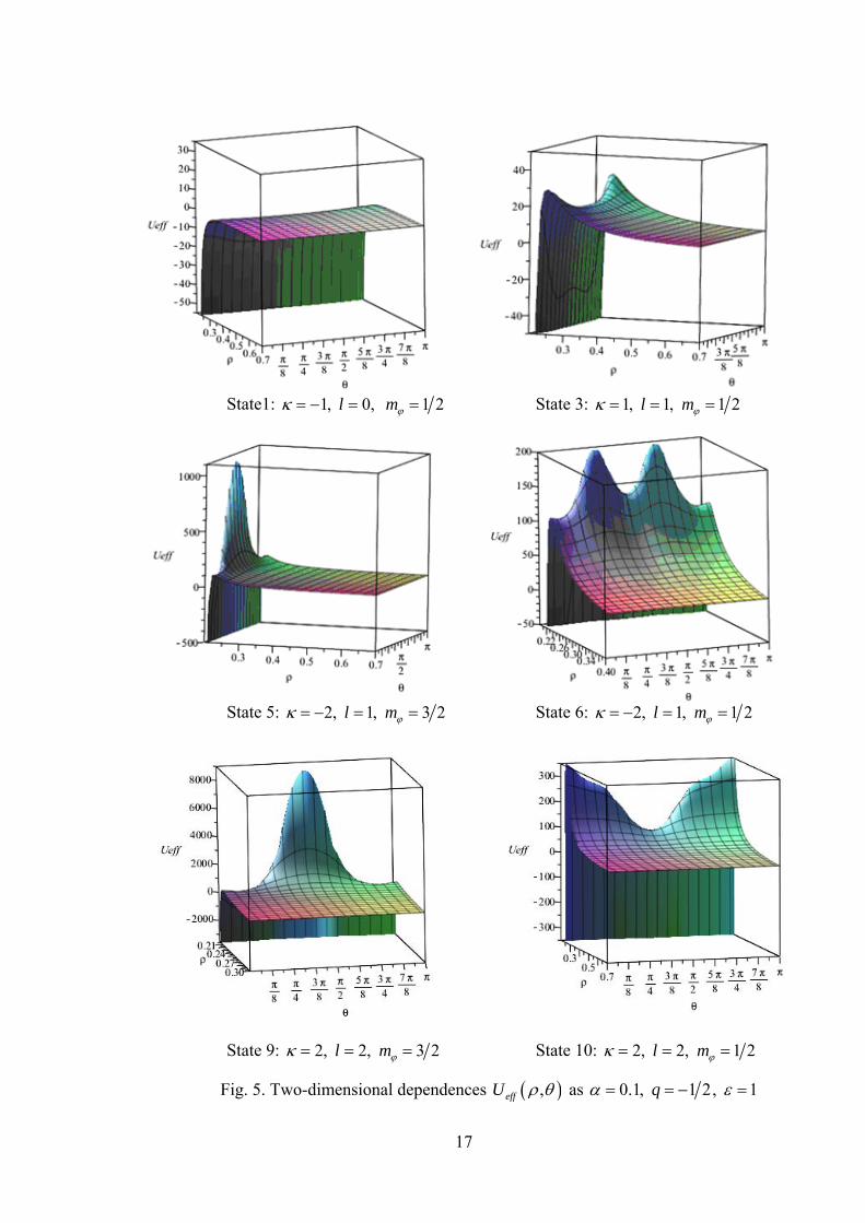
Fig. 5 presents two-dimensional dependences ,effU as 0.5q for the states of the

Dirac particle considered in fig.1.

For the states with 0l in front of the potential well (40) there exist essential repulsive

barriers. In all cases, the heights of the barriers notably depend on a polar angle .

State 1: 1, 0, 1 2l m

State 3: 1, 1, 1 2l m

14

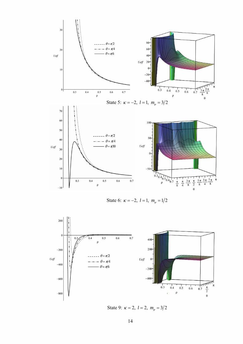
State 5: 2, 1, 3 2l m

State 6: 2, 1, 1 2l m

State 9: 2, 2, 3 2l m

15

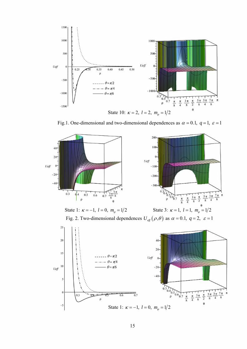
State 10: 2, 2, 1 2l m

Fig.1. One-dimensional and two-dimensional dependences as 0.1, 1, 1q

State 1: 1, 0, 1 2l m State 3: 1, 1, 1 2l m

Fig. 2. Two-dimensional dependences ,effU as 0.1, 2, 1q

State 1: 1, 0, 1 2l m

16

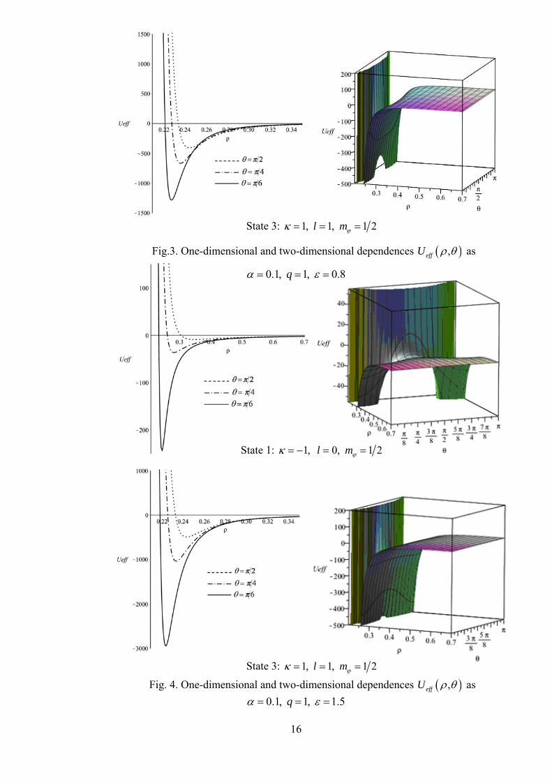
State 3: 1, 1, 1 2l m

Fig.3. One-dimensional and two-dimensional dependences ,effU as

0.1, 1, 0.8q

State 1: 1, 0, 1 2l m

State 3: 1, 1, 1 2l m

Fig. 4. One-dimensional and two-dimensional dependences ,effU as

0.1, 1, 1.5q

17

State1: 1, 0, 1 2l m State 3: 1, 1, 1 2l m

State 5: 2, 1, 3 2l m State 6: 2, 1, 1 2l m

State 9: 2, 2, 3 2l m State 10: 2, 2, 1 2l m

Fig. 5. Two-dimensional dependences ,effU as 0.1, 1 2, 1q

18

4. Cosmic censorship and a q - metric

The hypothesis of cosmic censorship proposed more than 40 years ago [22] prohibits the

existence of singularities, not shielded by event horizons. However, there is still no complete

proof of this hypothesis. Many researchers examine, along with black holes, the formation of

naked singularities, their stability and distinctive features during experimental observations (see,

for instance, [23] - [28]). It is shown in [29] that there exist static metrics with time-like

singularities which prove out to be completely non-singular when examining quantum

mechanics of spinless particles. In [30] , these results are validated as applied to the motion of

half-spin quantum-mechanical particles in the field of the Reissner-Nordström naked singularity.

For any Dirac particle irrespective of availability and sign of its electric charge, the Reissner-

Nordström naked singularity is separated by an infinitely large repulsive barrier.

20

3 1.

8effU

(41)

According to the vivid expression of the authors of [29], the existence of a repulsive

barrier covering the singularity does not threat the cosmic censorship.

Let us discuss the naked singularities of the static q-metric in the similar way.

In case of the oblate mass distribution 0,q , we see from (36), (38) that the naked

singularities of a q -metric are covered with infinitely large repulsive barriers which agrees with

the hypothesis of the cosmic censorship. The exception are the poles and, as *0 q q , some

points i for the states of a particle with 3 2j . In this case, in points i instead of a

repulsive barrier there exists a potential well of the form (39) with the coefficient 1L , allowing

the existence of stationary bound states of Dirac particles. At the poles, there exists an infinitely

deep potential well (37). The effect of the poles and the points i as 3 2j and *0 q q

on the conclusion of compliance with the hypothesis of cosmic censorship must be determined in

more accurate quantum-mechanical calculations of solution to the Dirac equation.

In case of the prolate mass distribution 1,0q along the axial axis, the naked

singularities for some intervals are not covered with a repulsive barrier. However, the view of

the leading term (40) as lim1 q q testifies to the existence possibility of stationary bound

states of a Dirac particle.

In the interval lim 0q q , there are implemented the conditions of a quantum-

mechanical “fall” of a Dirac particle to the outer singularity 2 .

19

Conclusions

The quantum-mechanical motion of half-spin particles was examined in the field of

naked singularities of the static q-metric formed by mass distribution with a quadrupole moment.

The analysis was performed by means of the method of effective potentials of the Dirac equation

generalized for the case when radial and angular variables are not separated. In order to obtain

effective potentials, the self-conjugate Dirac Hamiltonian in the field of the naked singularities

of the q-metric was determined.

The q-metric is transformed to the Schwarzschild metric as 0q . The leading term of

the effective potential for the Schwarzschild metric near the event horizon is

2 2

22

12

8 .2

SeffU

(42)

The expression (42) testifies to the fact that the motion of the Dirac particle in the Schwarzschild

field is implemented in the mode of a “fall” to the event horizon [31].

The transition from the spherical-symmetric to the deformed mass distribution in the

source of the gravitational field leads to essential variations in the motion of the Dirac particle.

The motion conditions of a half-spin particle strongly differ as well subject to the form of mass

distribution.

For the prolate mass distribution along the axial axis of mass distribution

lim lim1 , 1q q q , the view of the leading term of the effective potential near the outer

naked singularity (40) with the coefficient N in table 2 testifies to the existence possibility of

stationary bound states of half-spin particles. An analogy can be the existence of the energy

spectrum of electrons in the field of the singular Coulomb potential in hydrogen-like atoms with

137Z (the Sommerfeld formula). As lim 0q q , there exist the conditions for a quantum-

mechanical “fall” of particles to the outer singularity 2 .

For the oblate mass distribution along the axial axis 0 q , the effective potential

near the outer naked singularity has a more complicate form. The naked singularities are

separated by infinitely high repulsive barriers (36), (38) with the subsequent transition to a

potential well whose depth increases while moving along the angle from the equator to the poles.

For the state with 0l , the potential well can appear at a certain value of min and min .

Generally speaking, such a potential agrees with the cosmic censorship since the naked

singularities of the q-metric are shielded by an impenetrable quantum-mechanical barrier. The

20

exception are the poles and, as *0 q q , some points i for the states of the particle with

3 2j . In these points, the leading terms of the effective potentials are attractive potentials

(37), (39). The potentials with the leading term (39) allow the existence possibility of stationary

bound states of Dirac particles. Only at the poles 0 , there exist conditions for a

quantum-mechanical “fall” of the particle to the outer singularity 2 . The effect of the poles

and the finite number of points i on the penetrability characteristics of the barriers must be

evaluated in more accurate quantum-mechanical calculations of the solution to the Dirac

equation in the field of the naked singularities of the q-metric. But we can already say that these

characteristics will be changed insignificantly.

Thereby for the oblate mass distribution 0 q , the naked singularities of the q-

metric are separated from the Dirac particle by infinitely large repulsive barriers that is

conformed with cosmic censorship. For a prolate mass distribution lim lim1 , 1q q q , the

singularity of the effective potentials enables the possibility of existence of stationary bound

states of half-spin particles. The conditions of a quantum-mechanic “fall” of the particles to the

outer singularity 2 are implemented as lim 0q q only.

Acknowledgements

The authors would like to thank A.L. Novoselova for the essential technical support while

elaborating the paper.

21

References

[1] H.Weyl, Ann. Physik 54, 117 (1917).

[2] H. Quevedo, Gen. Rel. Grav. 43 1141 (2011).

[3] H. Quevedo, Forts. Physik 38 (1990) 733.

[4] H. Quevedo, Int. J. Mod. Phys. D 20 1779 (2011).

[5] D. Malafarina, Conf. Proc. C0405132, 273 (2004).

[6] S. Parnovsky, Zh. Eksp. Teor. Fiz. 88, 1921 (1985); JETP 61, 1139 (1985).

[7] D. Papadopoulos, B. Stewart, L. Witten, Phys. Rev. D 24, 320 (1981).

[8] L. Herrera and J. L. Hernandez-Pastora, J. Math. Phys. 41, 7544 (2000).

[9] L. Herrera, G. Magli and D. Malafarina, Gen. Rel. Grav. 37, 1371 (2005).

[10] N. Dadhich and G. Date, (2000), arXiv:gr-qc/0012093.

[11] H. Kodama and W. Hikida, Class. Quantum Grav. 20, 5121 (2003).

[12] A. N. Chowdhury, M. Patil, D. Malafarina, and P. S. Joshi, Phys. Rev. D 85,

104031 (2012).

[13] K. Boshkayev, E. Gasperin, A. C. Gutierrez-Pineres, H. Quevedo and S.

Toktarbay, Phys. Rev. D 93. 024024 (2016), arxiv: 1509.03827 [gr-qc].

[14] S.Toktarbay, H.Quevedo, Gravit. Cosmol. (2014) 20: 252, arxiv: 1510.04155 [gr-

qc].

[15] M.V.Gorbatenko, V.P.Neznamov. Phys. Rev. D82, 104056 (2010).

[16] M.V.Gorbatenko, V.P.Neznamov. Phys. Rev. D83, 105002 (2011).

[17] M.V.Gorbatenko, V.P.Neznamov. Journal of Modern Physics, 6, 303-326 (2015);

arxiv: 1107.0844 [gr-qc].

[18] J.Schwinger. Phys. Rev. vol. 130, 800-805 (1963).

[19] S.R.Dolan. Trinity Hall and Astrophysics Group, Cavendish Laboratory.

Dissertation, 2006.

[20] D.R. Brill, J.A. Wheeler. Rev. of Modern Physics, 29, 465-479 (1957).

[21] L.D.Landau, E.M.Lifshitz. Quantum Mechanics. Nonrelativistic Theory,

Fizmatlit, Moscow (1963), (in Russian); [L.D.Landau and E.M.Lifshitz. Quantum

Mechanics. Nonrelativistic Theory, Pergamon Press, Oxford (1965)].

[22] R.Penrose, Rivista del Nuovo Cimento, Serie I, 1, Numero Speciale: 252 (1969).

[23] R.S.Virbhadra, D.Narasimba and S.M.Chitre, Astron. Astrophys. 337, 1- 8 (1998).

[24] K.S.Virbhadra and G.F.R.Ellis, Phys. Rev. D65, 103004 (2002).

[25] K.S.Virbhadra, C.R.Keeton, Phys. Rev. D77, 124014 (2008).

22

[26] D.Dey, K.Bhattacharya and N.Sarkar, Phys. Rev. D88, 083532 (2013).

[27] P.S.Joshi, D.Malafaxina and Maragan, Class. Quant. Grav. 31, 015002 (2014).

[28] A.Goel, R.Maity, P.Roy, Tsarkar, arxiv: 1504.01302 [gr-qc].

[29] G.T.Horowitz and D.Marolf, Phys. Rev. D, 52, 5670 (1995).

[30] М.V.Gorbatenko, V.P.Neznamov, Eu.Y.Popov, I.I.Safronov, arxiv: 1511.05482

[gr-qc].

[31] М.V.Gorbatenko, V.P.Neznamov, Eu.Y.Popov, Journal of Physics: Conference

Series 678 (2016) 012037 doi:10.1088/1742-6596/678/1/012037, arxiv: 1511.05058

[gr-qc].