Resonance and Singularities

Henk W. Broer and Gert Vegter∗

To Jan Karel Lenstra, on the occasion of his retirement.

August 18, 2011

Abstract

The phenomenon of resonance will be dealt with from the viewpoint of dy-namical systems depending on parameters and their bifurcations. Resonancephenomena are associated to open subsets in the parameter space, while theircomplement corresponds to quasi-periodicity and chaos. The latter phenom-ena occur for parameter values in fractal sets of positive measure. We de-scribe a universal phenomenon that plays an important role in modelling.This paper gives a summary of the background theory, veined by examples.

1 What is resonance?

A heuristic definition of resonance considers a dynamical system, usually depend-ing on parameters, with several oscillatory subsystems having a rational ratio offrequencies and a resulting combined and compatible motionthat may be ampli-fied as well. Often the latter motion is also periodic, but it can be more compli-cated as will be shown below. We shall take a rather eclectic point of view, dis-cussing several examples first. Later we shall turn to a number of universal cases,these are context-free models that occur generically in anysystem of sufficientlyhigh-dimensionial state and parameter space.

Among the examples are the famous problem of Huygens’s synchronizing clocksand that of the Botafumeiro in the Cathedral of Santiago de Compostela, but also

∗Johann Bernoulli Institute for Mathematics and Computer Science, University of Groningen,PO Box 407, 9700 AK Groningen, The Netherlands

1

R

ωα

R

ωα

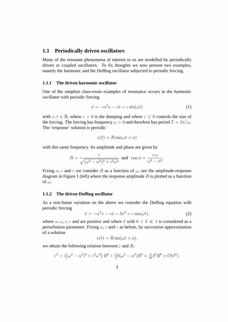
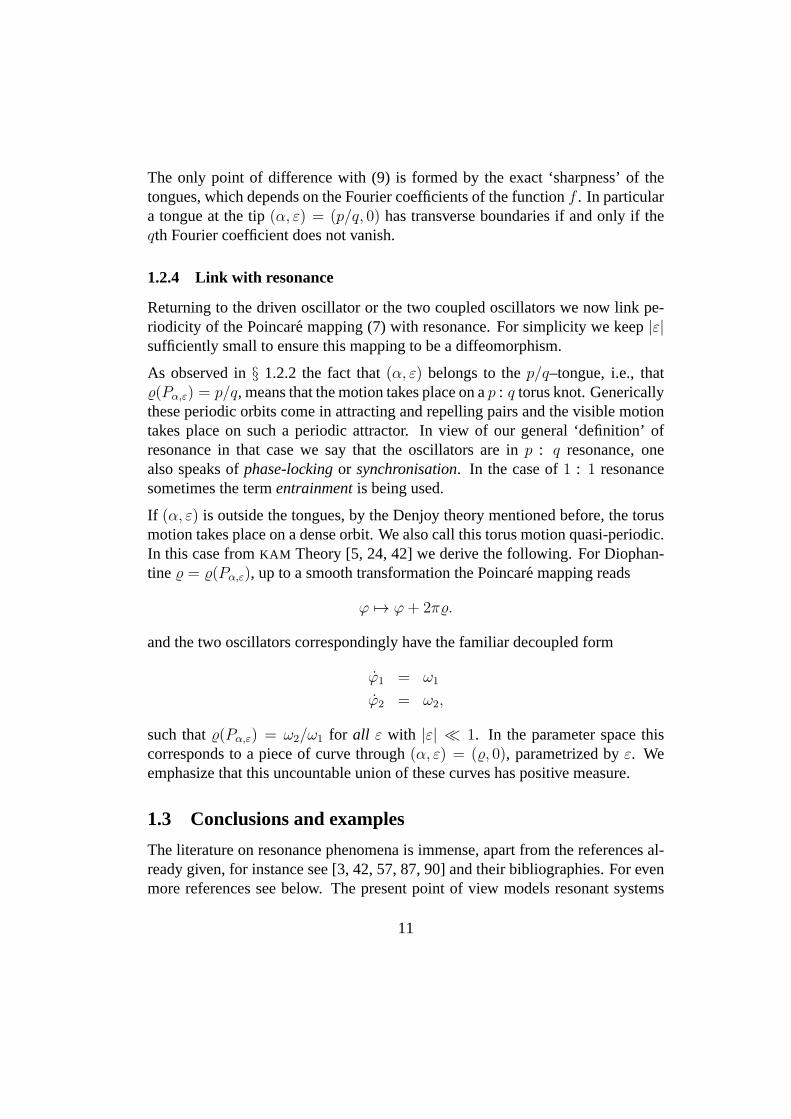
Figure 1: Amplitude-response diagrams in the(ω,R)–plane. Left: the periodi-cally driven harmonic oscillator (1) and right: the driven Duffing oscillator (2).

we briefly touch on tidal resonances in the planetary system.As universal modelswe shall deal with the Hopf–Neımark–Sacker bifurcation and the Hopf saddle-node bifurcation for mappings. The latter two examples form‘next cases’ in thedevelopment of generic bifurcation theory. The termuniversalrefers to the con-text independence of their occurrence: in any with certain generic specificationsthese bifurcations occur in a persistent way. We witness an increase in complex-ity in the sense that in the parameter space the resonant phenomena correspondto an open & dense subset union of tongues, while in the complement of this anowhere dense set of positive measure exists, corresponding to multi- or quasi-periodic dynamics. This nowhere dense set has a fractal geometry in a sense thatwill be explained later. From the above it follows that this global array of reso-nance tongues and fractal geometry has a universal character. As we shall see,both locally and globally Singularity Theory can give organizing principles. Itshould be noted at once that next to periodic and quasi-periodic dynamics alsoforms of chaotic dynamics will show up.

Remark. In many cases the resonant bifurcations are repeated at eversmallerscales inside the tongues, leading to an infinite regress. Then we have to extendthe notion of open & dense toresidual and that of nowhere dense tomeagre.Here a residual set contains a countable intersection of open & dense sets, whilea meagre set is a countable union of nowhere dense sets. One sometimes alsospeaks in terms ofGδ– orFσ–sets, respectively [72].

2

1.1 Periodically driven oscillators

Many of the resonant phenomena of interest to us are modelledby periodicallydriven or coupled oscillators. To fix thoughts we now presenttwo examples,namely the harmonic and the Duffing oscillator subjected to periodic forcing.

1.1.1 The driven harmonic oscillator

One of the simplest class-room examples of resonance occursin the harmonicoscillator with periodic forcing

x = −α2x− cx+ ε sin(ωt) (1)

with x, t ∈ R, wherec > 0 is the damping and whereε ≥ 0 controls the size ofthe forcing. The forcing has frequencyω > 0 and therefore has periodT = 2π/ω.The ‘response’ solution is periodic

x(t) = R sin(ωt+ φ)

with this same frequency. Its amplitude and phase are given by

R =ε√

(ω2 − α2)2 + c2ω2and tanφ =

c ω

ω2 − α2.

Fixing α, c andε we considerR as a function ofω, see the amplitude-responsediagram in Figure 1 (left) where the response amplitudeR is plotted as a functionof ω.

1.1.2 The driven Duffing oscillator

As a non-linear variation on the above we consider the Duffingequation withperiodic forcing

x = −α2x− cx− δx3 + ε sin(ωt), (2)

whereα, ω, c, ε and are positive and whereδ with 0 < δ ≪ 1 is considered as aperturbation parameter. Fixingα, c andε as before, by successive approximationof a solution

x(t) = R sin(ωt+ φ),

we obtain the following relation betweenε andR:

ε2 =((ω2 − α2)2 + c2ω2

)R2 + 3

2δ(ω2 − α2)R4 + 9

16δ2R6 +O(δ3),

3

asδ ↓ 0, with a similar approximation for the phaseφ, compare with Stoker [86],also see [24]. In Figure 1 (right) we depict the corresponding curve in the(ω,R)–plane, which now no longer is a graph.

Remarks

- One of the exciting things about resonance concerns the peaks of the ampli-tudeR that can be quite high, even whereε is still moderate. Systems like(1) and (2) form models ormetaphorsfor various resonance phenomena indaily life. In many cases high resonance peaks one needs to ‘detune’ awayfrom the resonance value corresponding to the peak, think ofa marchingplatoon of soldiers that have to go out of pace when crossing abridge.

- In other cases, like when ‘tuning’ the radio receiver to a certain channel,one takes advantage of the peak.

- It should be noted that the nonlinear (2) dynamically is farricher than thelinear case (1), e.g., see [57] and references therein.

1.1.3 Geometrical considerations

In both cases of the driven oscillators witnessed above the state space isR2×T1 ={x, y, z}, where

x = y

y = a(x, y, δ) + ε sin z

z = ω,

with a(x, y, δ) = −α2x − cy − δx3, whereδ = 0 in the harmonic example. Thesecond factor is the circleT1 = R/(2πZ) which takes into account the periodicityof the systems inz. The response motion of the formx(t) = R sin(ωt + φ) thencorresponds to a closed curve

xyz

(t) =

R sin(ωt+ φ)ωR cos(ωt+ φ)

ωt+ φ

. (3)

This closed curve, when projected onto the(x, y)–plane, exactly forms an ellipse.

4

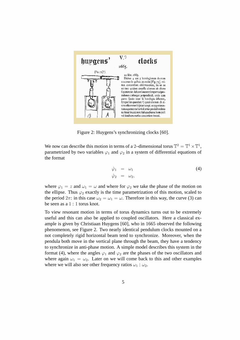
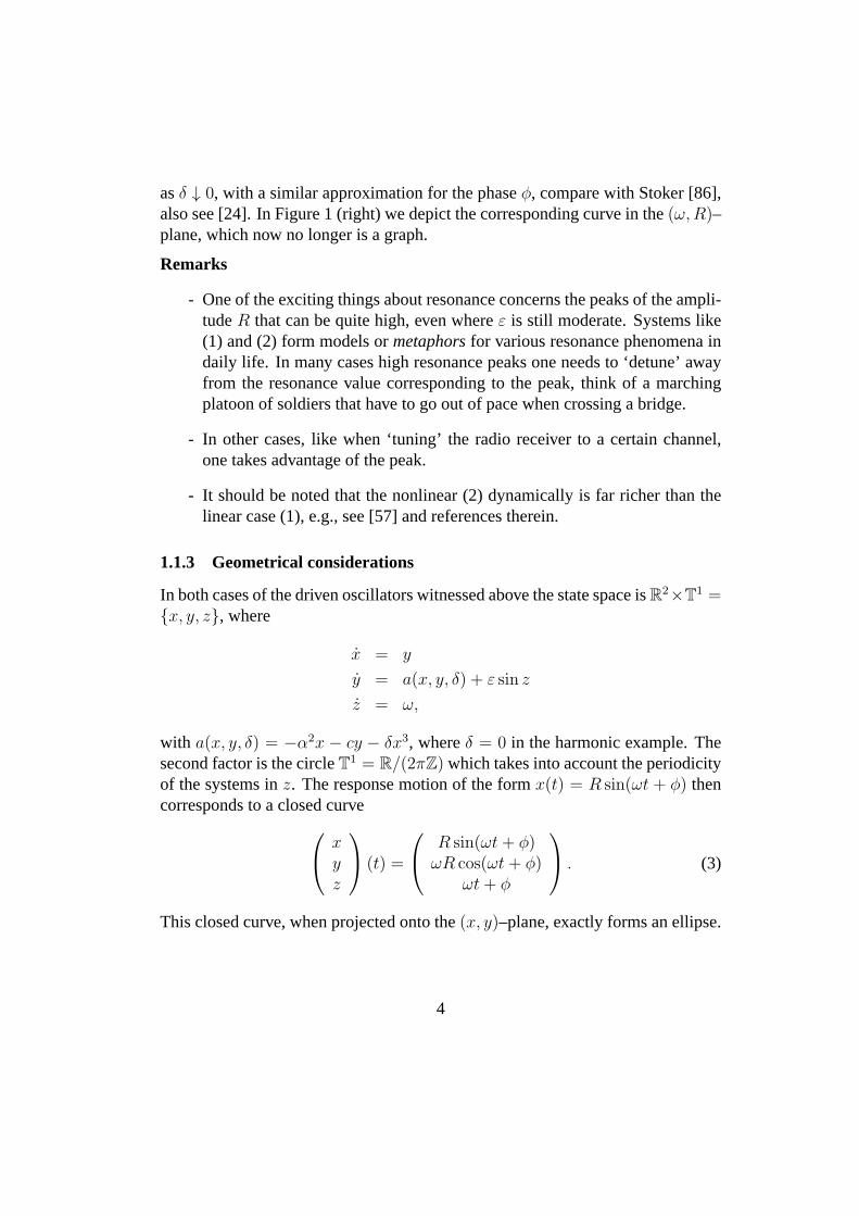
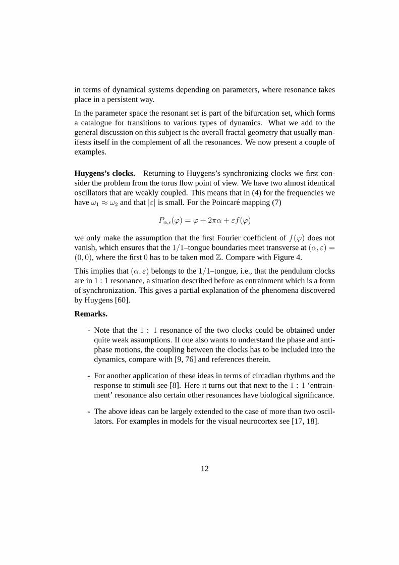
Figure 2: Huygens’s synchronizing clocks [60].

We now can describe this motion in terms of a2–dimensional torusT2 = T1×T1,parametrized by two variablesϕ1 andϕ2 in a system of differential equations ofthe format

ϕ1 = ω1 (4)

ϕ2 = ω2,

whereϕ1 = z andω1 = ω and where forϕ2 we take the phase of the motion onthe ellipse. Thusϕ2 exactly is the time parametrization of this motion, scaled tothe period2π: in this caseω2 = ω1 = ω. Therefore in this way, the curve (3) canbe seen as a1 : 1 torus knot.

To view resonant motion in terms of torus dynamics turns out to be extremelyuseful and this can also be applied to coupled oscillators. Here a classical ex-ample is given by Christiaan Huygens [60], who in 1665 observed the followingphenomenon, see Figure 2. Two nearly identical pendulum clocks mounted on anot completely rigid horizontal beam tend to synchronize. Moreover, when thependula both move in the vertical plane through the beam, they have a tendencyto synchronize in anti-phase motion. A simple model describes this system in theformat (4), where the anglesϕ1 andϕ2 are the phases of the two oscillators andwhere againω1 = ω2. Later on we will come back to this and other exampleswhere we will also see other frequency ratiosω1 : ω2.

5

ϕϕϕϕϕϕϕϕϕϕϕϕϕϕϕϕϕϕϕϕϕϕϕ

P (ϕ)P (ϕ)P (ϕ)P (ϕ)P (ϕ)P (ϕ)P (ϕ)P (ϕ)P (ϕ)P (ϕ)P (ϕ)P (ϕ)P (ϕ)P (ϕ)P (ϕ)P (ϕ)P (ϕ)P (ϕ)P (ϕ)P (ϕ)P (ϕ)P (ϕ)P (ϕ)

Figure 3: Poincare mapping of a torus flow [42].

1.2 Torus flows and circle mappings

In this section we turn to the dynamics on the2–dimensional torusT2 from § 1.1.3for its own sake, introducing the weakly coupled system

ϕ1 = ω1 + εf1(ϕ1, ϕ2) (5)

ϕ2 = ω2 + εf2(ϕ1, ϕ2).

Heref1 andf2 are2π–periodic functions in both variables. Also we use a pa-rameterε to control the strength of the coupling. Forε = 0 we retrieve theformat (4). IfT1 andT2 are the respective periods of oscillation, thenω1 = 2π/T1

andω2 = 2π/T2. We first define the Poincare mapping from the circleT1 to itselfand then introduce the rotation number.

1.2.1 The Poincare mapping

If in (5) the size|ε| of the coupling is not too large, a first-return Poincare mapping

P : T1 −→ T1 (6)

is defined, as we shall explain now, also see Figure 3. Withoutrestricting gen-erality we can take the generating circle to beT1 × {0}. Baptisingϕ = ϕ1 forsimplicity, we follow the integral curve from the initial state (ϕ1, ϕ2) = (ϕ, 0)until (ϕ1, ϕ2) = (P (ϕ), 0), counting mod2πZ. It is easy to see thatP − Id shouldbe a periodic function inϕ, which givesP the general form

P : ϕ 7→ ϕ+ 2πα + εf(ϕ), (7)

whereα = ω2/ω1 and wheref is a2π–periodic function.

6

Consideration of theT1–dynamics generated by iteration ofP gives a lot of in-formation about the originalT2–flow, in particular its asymptotic properties ast → ∞. For instance, a fixed point attractor ofP corresponds to an attractingperiodic orbit of the flow which forms a1 : 1 torus knot as we saw at the end of§ 1.1. Similarly a periodic attractor ofP of periodq corresponds to an attractingperiodic orbit of the flow. In general, periodicity will be related to resonance, butto explain this further we need the notion of rotation number.

1.2.2 Rotation number

For orientation-preserving homeomorphismsP : T1 −→ T1 Poincare has leftus the extremely useful concept ofrotation number (P ), which describes theaverage amount of rotation as follows:

(P ) =1

2πlimn→∞

1

n(P )n(ϕ)modZ. (8)

HereP : R −→ R is a (non-unique) lift ofP which makes the diagram

RP−−−→ R

pr

yypr

T1 P−−−→ T1

commute, wherepr : R −→ T1 is the natural projectionϕ 7→ eiϕ. This meansthat in the formula (8) we do not count modulo2π, but keep counting inR.

From [52, 71] we quote a number of properties of(P ):

1. (P ) depends neither on the choice of the liftP nor on the choice ofϕ;

2. (P ) is invariant under topological conjugation. This means that if h :T1 −→ T1 is another orientation-preserving homeomorphism, then

(hPh−1) = (P );

3. If P : ϕ 7→ ϕ+ 2πα is a rigid rotation then (P ) = αmodZ.

4. (P ) ∈ Q precisely whenP has a periodic point. Moreover,(P ) = p/qwith p andq relatively prime corresponds to ap : q torus knot.

7

3

2.5

2

1.5

1

0.5

0 1/8 1/7 1/6 1/5 2/9 1/4 2/7 1/3 3/8 2/5 3/7 4/9 1/20

-1/2 -4/9 -3/7 -1/4-2/7-1/3-3/8-2/5 -1/8-1/7-1/6-1/5-2/9

ε

α

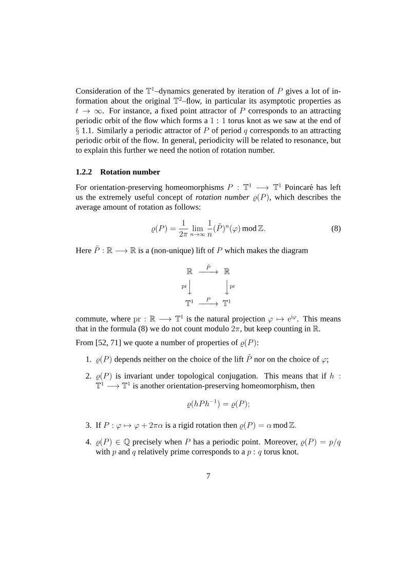
Figure 4: Resonance tongues in the Arnold family (9).

5. If P is of classC2 and(P ) = α for α ∈ R \ Q, then, by a result ofDenjoy, the mappingP is topologically conjugated to the rigid rotationϕ 7→ϕ+ 2πα.

Recall that in that case any orbit{P n(ϕ)}n∈Z forms a dense subset ofT1.The corresponding dynamics is calledquasi-periodic.

6. If P depends continuously on a parameter, then so does(P ).

1.2.3 The Arnold family of circle mappings

A famous example of maps exhibiting resonance is formed by the Arnold family

Aα,ε : ϕ 7→ ϕ+ 2πα + ε sinϕ (9)

of circle mappings. So this is the general format (7) where wechosef(ϕ) =sinϕ.1

Periodicity. It is instructive to consider the fixed points of (9), given bytheequation

Aα,ε(ϕ) = ϕ,

or, equivalently,

sinϕ = −2πα

ε.

1For simplicity we take|ε| < 1 which ensures that (9) is a circle diffeomorphism; for|ε| ≥ 1the mapping becomes a circleendomorphismand the current approach breaks down.

8

-0.6

-0.4

-0.2

0

0.2

0.4

0.6

-0.4 -0.2 0 0.2 0.4α

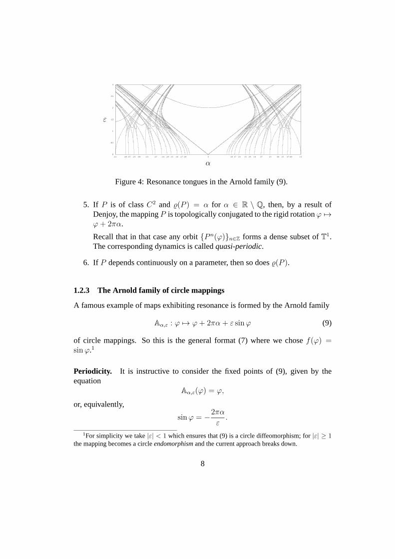
Figure 5: Devil’s staircase related to the Arnold family (9). For smallε0 > 0 therotation number (Aα,ε0) is depicted as a graph ofα ∈ [0, 1].

A brief graphical inspection reveals thatmod 2πZ this equation has exactly twosolutions for

|ε| > 2π|α|.In Figure 4 this region, bounded by the two straight linesε = ±2πα, is depictedfor ε > 0. It is not hard to see that one of the fixed points is attractingand the otherrepelling. At the boundary|ε| = 2π|α| these annihilate one another in a saddle-node bifurcation. For the entire region|ε| ≥ 2π|α| one has (Aα,ε) = 0modZ.This region is called the Arnold tongue of rotation number0.

From the properties of§ 1.2.2 it follows that, for(α, ε) = (p/q, 0) with p andqrelatively prime, one has(Aα,ε) = p/q. One can show that from each(α, ε) =(p/q, 0) an Arnold tongue emanates, in which for all the parameter points (α, ε)one has (Aα,ε) = p/q, see Figure 4. The ‘sharpness’, i.e., the order of contactof the boundaries of thep/q–tongue at(α, ε) = (p/q, 0) exactly is of orderq,see [1, 3, 36].

Fixing ε = ε0 > 0 small, we consider the graph ofα 7→ (Aα,ε0). By anothergeneral property of§ 1.2.2, this function is continuous. Moreover, for every ratio-nal valuep/q it is constant on some plateau, corresponding to thep/q–tongue, seeFigure 4. The total result is a devil’s staircase as depictedin Figure 5.

Quasi-periodicity. In between the tongues the rotation number(Aα,ε) is irra-tional and by the properties of§ 1.2.2 we know that the corresponding iterationdynamics ofA is quasi-periodic and that each individual orbits densely fills T1.

9

Open & dense versus nowhere dense.In general the(α, ε)–plane of parame-ters contains a catalogue of the circle dynamics. Again fixing ε = ε0 > 0 small,consider the corresponding horizontal line in the(α, ε)–plane of parameters. Wewitness the following, also see Figure 5 and compare with [36] and referencestherein. The periodic case corresponds to an open & dense subset of the line, andthe quasi-periodic case to a nowhere dense subset, which in the 1–dimensionalsituation is a Cantor set.

Diophantic rotation numbers. Quasi-periodicity corresponds to = (Pα,ε0) /∈Q. If we restrict even further to Diophantineby requiring that for constantsτ > 2 andγ > 0, for all rationalsp/q

∣∣∣∣−p

q

∣∣∣∣ ≥γ

|q|τ , (10)

the conjugations ofPα,ε0 with the rigid rotationϕ 7→ ϕ + 2π can be takensmooth [1, 42]. The rotation numbers satisfying (10) form a Cantor subset of theformer, which has positive Lebesgue measure, which, by choosingγ = γ(ε0) =O(ε0), can be shown to tend to full measure asε0 → 0. A fortiori this holds forthe original Cantor set given by(Pα,ε0) /∈ Q.

Fractal geometry. The Cantor sets under consideration, since they have positiveLebesgue measure, have Hausdorff dimension equal to1. Moreover Cantor setshave topological dimension0, since they are totally disconnected: every point hasarbitrarily small neighbourhoods with empty boundary. Thefact that the Haus-dorff dimension strictly exceeds the topological dimension is a characterisation offractals, see page 15 of [66]. So our Cantor sets are fractals.They also show a lotof self-similarity, a property shared with many other fractals.

Beyond the Arnold family (9) . . . The decomposition of the parameter space inan open & dense set on the one hand, versus a nowhere dense, fractal set of posi-tive measure turns out to be universal, also see [36]. To begin with, any arbitrarysmooth (Poincare) circle mapping of the more general format (7)

Pα,ε : ϕ 7→ ϕ+ 2πα + εf(ϕ)

turns out to have an array of resonance tongues similar to theArnold family (9),forming an open & dense set that corresponds to periodicity,with a fractal comple-ment which is nowhere dense and of positive measure that corresponds to quasi-periodicity.

10

The only point of difference with (9) is formed by the exact ‘sharpness’ of thetongues, which depends on the Fourier coefficients of the functionf . In particulara tongue at the tip(α, ε) = (p/q, 0) has transverse boundaries if and only if theqth Fourier coefficient does not vanish.

1.2.4 Link with resonance

Returning to the driven oscillator or the two coupled oscillators we now link pe-riodicity of the Poincare mapping (7) with resonance. For simplicity we keep|ε|sufficiently small to ensure this mapping to be a diffeomorphism.

As observed in§ 1.2.2 the fact that(α, ε) belongs to thep/q–tongue, i.e., that(Pα,ε) = p/q, means that the motion takes place on ap : q torus knot. Genericallythese periodic orbits come in attracting and repelling pairs and the visible motiontakes place on such a periodic attractor. In view of our general ‘definition’ ofresonance in that case we say that the oscillators are inp : q resonance, onealso speaks ofphase-lockingor synchronisation. In the case of1 : 1 resonancesometimes the termentrainmentis being used.

If (α, ε) is outside the tongues, by the Denjoy theory mentioned before, the torusmotion takes place on a dense orbit. We also call this torus motion quasi-periodic.In this case fromKAM Theory [5, 24, 42] we derive the following. For Diophan-tine = (Pα,ε), up to a smooth transformation the Poincare mapping reads

ϕ 7→ ϕ+ 2π.

and the two oscillators correspondingly have the familiar decoupled form

ϕ1 = ω1

ϕ2 = ω2,

such that (Pα,ε) = ω2/ω1 for all ε with |ε| ≪ 1. In the parameter space thiscorresponds to a piece of curve through(α, ε) = (, 0), parametrized byε. Weemphasize that this uncountable union of these curves has positive measure.

1.3 Conclusions and examples

The literature on resonance phenomena is immense, apart from the references al-ready given, for instance see [3, 42, 57, 87, 90] and their bibliographies. For evenmore references see below. The present point of view models resonant systems

11

in terms of dynamical systems depending on parameters, where resonance takesplace in a persistent way.

In the parameter space the resonant set is part of the bifurcation set, which formsa catalogue for transitions to various types of dynamics. What we add to thegeneral discussion on this subject is the overall fractal geometry that usually man-ifests itself in the complement of all the resonances. We nowpresent a couple ofexamples.

Huygens’s clocks. Returning to Huygens’s synchronizing clocks we first con-sider the problem from the torus flow point of view. We have twoalmost identicaloscillators that are weakly coupled. This means that in (4) for the frequencies wehaveω1 ≈ ω2 and that|ε| is small. For the Poincare mapping (7)

Pα,ǫ(ϕ) = ϕ+ 2πα + εf(ϕ)

we only make the assumption that the first Fourier coefficientof f(ϕ) does notvanish, which ensures that the1/1–tongue boundaries meet transverse at(α, ε) =(0, 0), where the first0 has to be taken modZ. Compare with Figure 4.

This implies that(α, ε) belongs to the1/1–tongue, i.e., that the pendulum clocksare in1 : 1 resonance, a situation described before as entrainment which is a formof synchronization. This gives a partial explanation of thephenomena discoveredby Huygens [60].

Remarks.

- Note that the1 : 1 resonance of the two clocks could be obtained underquite weak assumptions. If one also wants to understand the phase and anti-phase motions, the coupling between the clocks has to be included into thedynamics, compare with [9, 76] and references therein.

- For another application of these ideas in terms of circadian rhythms and theresponse to stimuli see [8]. Here it turns out that next to the1 : 1 ‘entrain-ment’ resonance also certain other resonances have biological significance.

- The above ideas can be largely extended to the case of more than two oscil-lators. For examples in models for the visual neurocortex see [17, 18].

12

Resonances in the solar system.From ancient times on resonances have beenknown to occur in the solar system, which are more or less in the spirit of thepresent section. A well-known example is the orbital1 : 2 : 4 resonance ofJupiter’s moons Ganymede, Europa, and Io which was studied by De Sitter [83,84] using the ‘methodes nouvelles’ of Poincare [75]. The2 : 5 orbital resonancebetween Jupiter and Saturn is described by Moser et al. [68, 69, 81]. These andother resonances by certain authors are being held responsable for gaps in therings of Saturn and in the asteroid belt.

Another type of resonance is the spin-orbit resonance. As anexample thereof, theMoon is ‘captured by’ the Earth in a1 : 1 resonance: the lunar day with respectto the Earth is (approximately) equal to one month. Similarly Pluto and Charonhave caught each other in such a1 : 1 resonance: as an approximately rigid bodythe two orbit around the Sun. Interestingly, the planet Mercury is captured in a3: 2 spin-orbit resonance around the Sun [50].

Remarks.

- The spin orbit resonances are explained by tidal forces, for instance, therotation of the Moon has been slowed down to a standstill by tidal frictionbrought about largely by the reciprocal tidal forces exerted of Earth andMoon. Similarly the rotation of the Earth in the very long runwill be putto a stand still by the tidal forces of mainly the Moon. But probably by thattime the Sun has already turned into a red giant. . .

- This brings us to the subject of adiabatically changing systems as describedand summarized by Arnold [2, 3] and which may be used to model suchslow changes.2 One may perhaps expect that the3 : 2 spin orbit resonanceof Mercury in the very long run, and after quite a number of transitions, willevolve towards another1 : 1 resonance. This part of nonlinear dynamicalsystems still is largely unexplored.

2 Periodically driven oscillators revisited

We now return to periodically driven oscillators, showing that under certain cir-cumstances exactly the set-up of§ 1.2 applies.

2Mathematical ideas on adiabatic change were used earlier byRayleigh and Poincare and byLandau-Lifschitz.

13

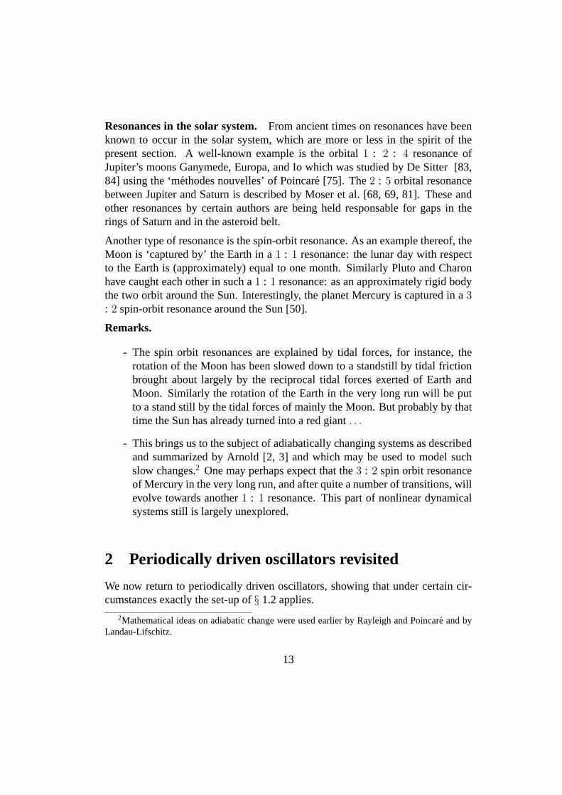
Figure 6: Botafumeiro in Santiago de Compostela.

As a motivating example we discuss the Botafumeiro in the cathedral of Santiagode Compostela, see Figure 6. Here a large incense container issuspended by apully in the dome where it can swing in the longitudinal direction of the church.A few men pull up the container when it approaches the ground and let go after,thereby creating a periodic forcing and in this way creatinga stable motion ofexactly twice the period of the forcing.

2.1 Parametric resonance

As another model consider the parametrically driven oscillator

x+ (a+ εf(t)) sin x = 0 (11)

with q(t + 2π) ≡ q(t), see [44]. Herea andε are considered as parameters.3 Forthe periodic functionf we have studied several examples, namely

f(t) = cos t and

= cos t+ 32 cos(2t) and

= signum(cos t),

corresponding to the Mathieu case, the Mathieu case modifiedby a higher har-monic, and the square case, respectively. In this setting the issue is whether thetrivial 2π–periodic solution

x(t) ≡ 0 ≡ x(t)

3For ‘historical’ reasons we use the lettera instead ofα2 as we did earlier.

14

0

1

2

3

4

5

6

-2 -1 0 1 2 3 4 5 60

1

2

3

4

5

6

-2 -1 0 1 2 3 4 5 6

0

1

2

3

4

5

6

-2 -1 0 1 2 3 4 5 6

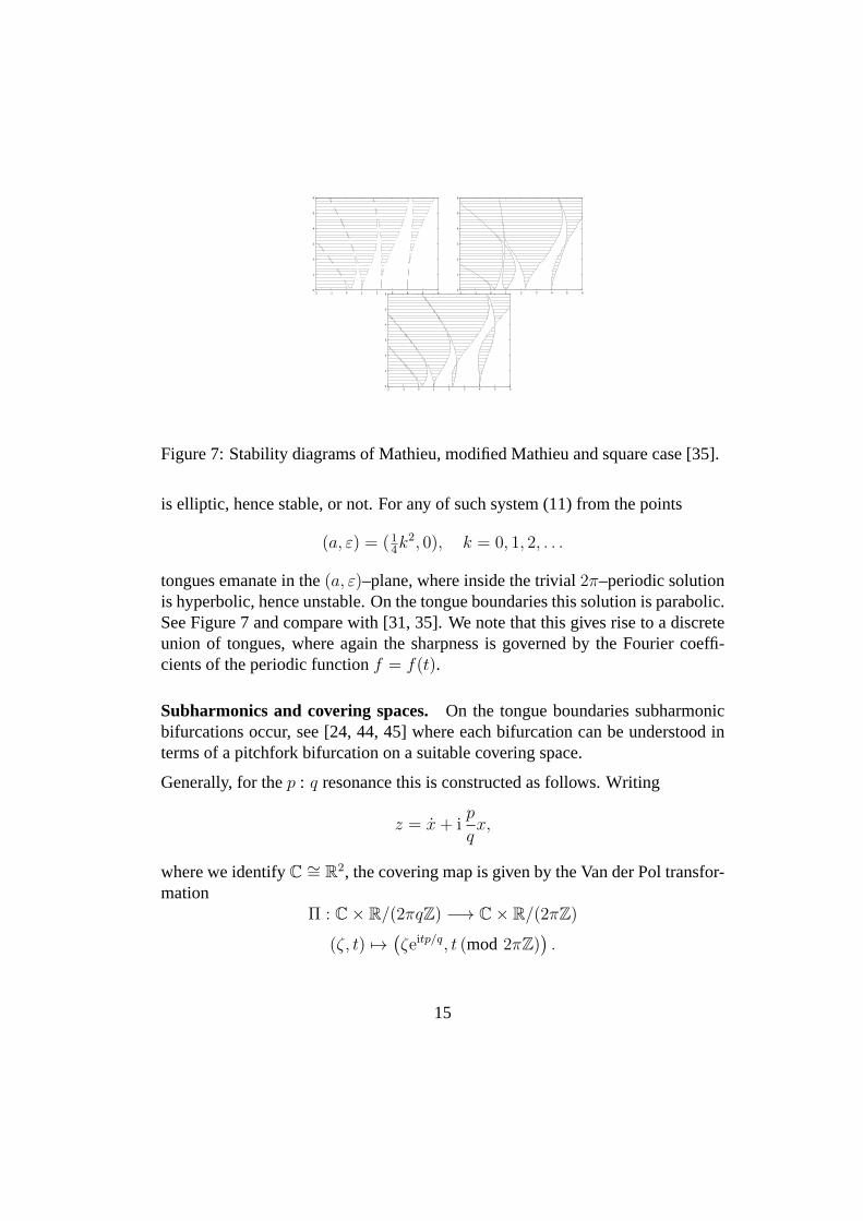
Figure 7: Stability diagrams of Mathieu, modified Mathieu and square case [35].

is elliptic, hence stable, or not. For any of such system (11)from the points

(a, ε) = (14k2, 0), k = 0, 1, 2, . . .

tongues emanate in the(a, ε)–plane, where inside the trivial2π–periodic solutionis hyperbolic, hence unstable. On the tongue boundaries this solution is parabolic.See Figure 7 and compare with [31, 35]. We note that this givesrise to a discreteunion of tongues, where again the sharpness is governed by the Fourier coeffi-cients of the periodic functionf = f(t).

Subharmonics and covering spaces.On the tongue boundaries subharmonicbifurcations occur, see [24, 44, 45] where each bifurcationcan be understood interms of a pitchfork bifurcation on a suitable covering space.

Generally, for thep : q resonance this is constructed as follows. Writing

z = x+ ip

qx,

where we identifyC ∼= R2, the covering map is given by the Van der Pol transfor-mation

Π : C× R/(2πqZ) −→ C× R/(2πZ)

(ζ, t) 7→(ζeitp/q, t (mod 2πZ)

).

15

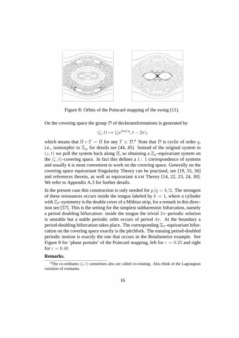
Figure 8: Orbits of the Poincare mapping of the swing (11).

On the covering space the groupD of decktransformations is generated by

(ζ, t) 7→ (ζe2πp/q, t− 2π),

which means thatΠ ◦ T = Π for anyT ∈ D.4 Note thatD is cyclic of orderq,i.e., isomorphic toZq, for details see [44, 45]. Instead of the original system in(z, t) we pull the system back alongΠ, so obtaining aZq–equivariant system onthe (ζ, t)–covering space. In fact this defines a1 : 1 correspondence of systemsand usually it is most convenient to work on the covering space. Generally on thecovering space equivariant Singularity Theory can be practised, see [19, 55, 56]and references therein, as well as equivariantKAM Theory [14, 22, 23, 24, 30].We refer to Appendix A.3 for further details.

In the present case this construction is only needed forp/q = k/2. The strongestof these resonances occurs inside the tongue labeled byk = 1, where a cylinderwith Z2–symmetry is the double cover of a Mobius strip, for a remark in this direc-tion see [57]. This is the setting for the simplest subharmonic bifurcation, namelya period doubling bifurcation: inside the tongue the trivial 2π–periodic solutionis unstable but a stable periodic orbit occurs of period4π. At the boundary aperiod-doubling bifurcation takes place. The correspondingZ2–equivariant bifur-cation on the covering space exactly is the pitchfork. The ensuing period-doubledperiodic motion is exactly the one that occurs in the Botafumeiro example. SeeFigure 8 for ‘phase portaits’ of the Poincare mapping, left forε = 0.25 and rightfor ε = 0.40

Remarks.4The co-ordinates(ζ, t) sometimes also are called co-rotating. Also think of the Lagrangean

variation of constants.

16

- The geometric complexity of the individual tongues in Figure 7 can be de-scribed by Singularity Theory; in fact it turns out that we are dealing withtypeA2k−1, see [35, 44].

- The parametric1 : 2 resonance sometimes also is called theparametric roll.By this mechanism ships have been known to capsize. . .

- In Figure 8 also invariant circles can be witnessed.KAM Theory, as dis-cussed before, in particular an application of Moser’s Twist Theorem [67],shows that the union of such invariant circles carrying quasi-periodic dy-namics has positive measure.

- In both cases the cloud of points5 is formed by just one or two orbits underthe iteration of the Poincare mapping. These clouds are associated to ho-moclinic orbits related to the upside down unstable periodic solution, whichgives rise to horseshoes. Therefore such an orbit is chaoticsince it haspositive topological entropy, see [42] and references therein. A classicalconjecture is that the cloud densely fills a subset of the plane of positiveLebesgue measure on which the Poincare mapping is ergodic [4].6

2.2 The Hill-Schrodinger equation

Another famous equation is a linearized version of (11) where the forcing term isquasi-periodic int:

x+ (a+ εf(t))x = 0, (12)

where nowf(t) = F (ω1t, ω2t, . . . , ωnt) for a functionF : Tn → R, see [32, 53,70]. As in the case of§ 1.2 the countable union of tongues again becomes open& dense and separated by a nowhere dense set of positive measure, determinedby Diophantine conditions. The geometry of the individual tongues for small|ε|is exactly as in the periodic case. For larger values of|ε| the situation is morecomplicated also involving non-reducible quasi-periodictori, compare with [34].

The equation (12) happens to be the eigenvalue equation of the 1–dimensionalSchrodinger operator with quasi-periodic potential. We here sketch how our geo-metric approach fits within the corresponding operator theory. This operator reads

(Hεfx) (t) = −x(t)− εf(t)x(t) (13)

5Colloquially often referred to as ‘chaotic sea’.6Also known as the metric entropy conjecture.

17

0.5

0.55

0.6

0.65

0.7

0.75

0.8

0.38 0.4 0.42 0.44 0.46 0.48 0.5 0.52

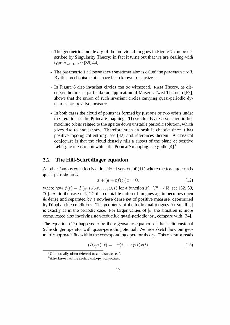
Figure 9: Devil’s staircase in the Schrodinger equation with quasi-periodic poten-tial: ω1 = 1 andω2 =

12(√5− 1), see [32].

with potentialεf ; it acts on wave functionsx = x(t) ∈ L2(R).

We like to note that in the corresponding literature usuallythe value ofε = ε0 6= 0is fixed and the intersection of the horizontal lineε = ε0 with a tongue is referredto asgap: it is a gap in the spectrum of the Schrodinger operator (13). The ap-proach with tongues and the results of [32] regarding theA2k−1–singularity there-fore leads to a generic gap closing theory.

Remarks.

- In the context of Schrodinger operators the letters are chosen somewhatdifferently. In particular, instead ofx(t) one often considersu(x), whichgives this theory a spatial interpretation. Also instead ofεf(t) one usesV (x), compare with [70].

- For a fixed valueε = ε0 the Diophantine Cantor set leads to Cantor spec-trum. The total picture is illustrated in the devil’s staircase of Figure 9,where we tookn = 2, ω1 = 1 andω2 =

12(√5− 1). The rotation number

is defined almost as before [32] as a function ofa.

- The nonlinear equation

x+ (a+ εf(t)) sin x = 0,

with q quasi-periodic is dealt with in [22]. In comparison with thecase ofperiodicf the averaged, approximating situation, is identical. However, theinfinite number of resonances and the Cantorization we saw before leads toan infinite regress of the bifurcation scenarios. For this use was made ofequivariant HamiltonianKAM Theory on a suitable covering space [24, 30].As a consequence the resonant set becomes residual and the quasi-periodicset meagre. Compare this with [7, 46, 47, 48] in the dissipative case.

18

x

y

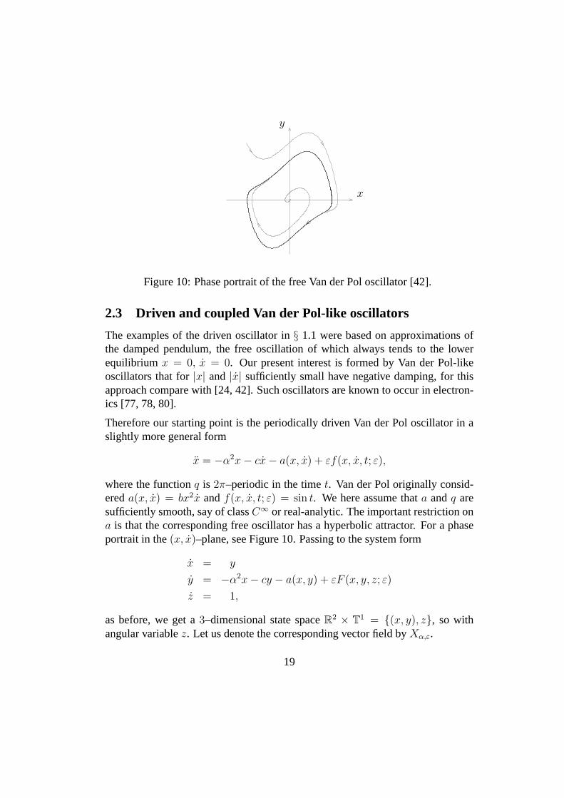
Figure 10: Phase portrait of the free Van der Pol oscillator [42].

2.3 Driven and coupled Van der Pol-like oscillators

The examples of the driven oscillator in§ 1.1 were based on approximations ofthe damped pendulum, the free oscillation of which always tends to the lowerequilibrium x = 0, x = 0. Our present interest is formed by Van der Pol-likeoscillators that for|x| and |x| sufficiently small have negative damping, for thisapproach compare with [24, 42]. Such oscillators are known to occur in electron-ics [77, 78, 80].

Therefore our starting point is the periodically driven Vander Pol oscillator in aslightly more general form

x = −α2x− cx− a(x, x) + εf(x, x, t; ε),

where the functionq is 2π–periodic in the timet. Van der Pol originally consid-ereda(x, x) = bx2x andf(x, x, t; ε) = sin t. We here assume thata andq aresufficiently smooth, say of classC∞ or real-analytic. The important restriction ona is that the corresponding free oscillator has a hyperbolic attractor. For a phaseportrait in the(x, x)–plane, see Figure 10. Passing to the system form

x = y

y = −α2x− cy − a(x, y) + εF (x, y, z; ε)

z = 1,

as before, we get a3–dimensional state spaceR2 × T1 = {(x, y), z}, so withangular variablez. Let us denote the corresponding vector field byXα,ε.

19

This brings us back to the general setting of a2–torus flow, with two phase anglesϕ1, ϕ2, e.g., withϕ1 the phase of the free oscillator, i.e., its time parametrizationscaled to period2π, andϕ2 = z. Forε = 0 we so obtain

ϕ1 = ω1

ϕ2 = ω2,

which is of the familiar format (4). From here the theory of§ 1.2 applies in alits complexity, with in the parameter space an open & dense, countable union ofresonances and a fractal set of positive measure regarding quasi-periodicity.

Similar results hold forn coupled Van der Pol type oscillators, now with statespaceTn, the cartesian product ofn copies ofT1. Next to periodic and quasi-periodic motion, now also chaotic motions occur, see [42] and references therein.

3 Universal studies

Instead of studying classes of driven or coupled oscillators we now turn to a fewuniversal cases of ‘generic’ bifurcations. The first of these is the Hopf-Neımark-Sacker bifurcation for diffeomorphisms, which has occurrence codimension1.This means that the bifurcation occurs persistently in generic 1–parameter fami-lies. However, the open & dense occurrence of countably manyresonances andthe complementary fractal geometry of positive measure in the bifurcation set areonly persistent in generic2–parameter families. A second bifurcation we study isthe Hopf saddle-node bifurcation for diffeomorphisms where we use3 parametersfor describing the persistent complexity of the bifurcation set.

3.1 The Hopf-Neımark-Sacker bifurcation

We start with the Hopf-Neımark-Sacker bifurcation for diffeomorphisms, but alsodiscuss certain consequences for systems of differential equations. As an exampleto illustrate our ideas consider the following Duffing–Van der Pol–Lienard typedriven oscillator

x+ (ν1 + ν3x2)x+ ν2x+ ν4x

3 + x5 = ε(1 + x6) sin t, (14)

the coefficients of which can be considered as parameters. Note that for the freeoscillator atν1 = 0 the eigenvalues of the linear part at(x, x) = (0, 0) cross the

20

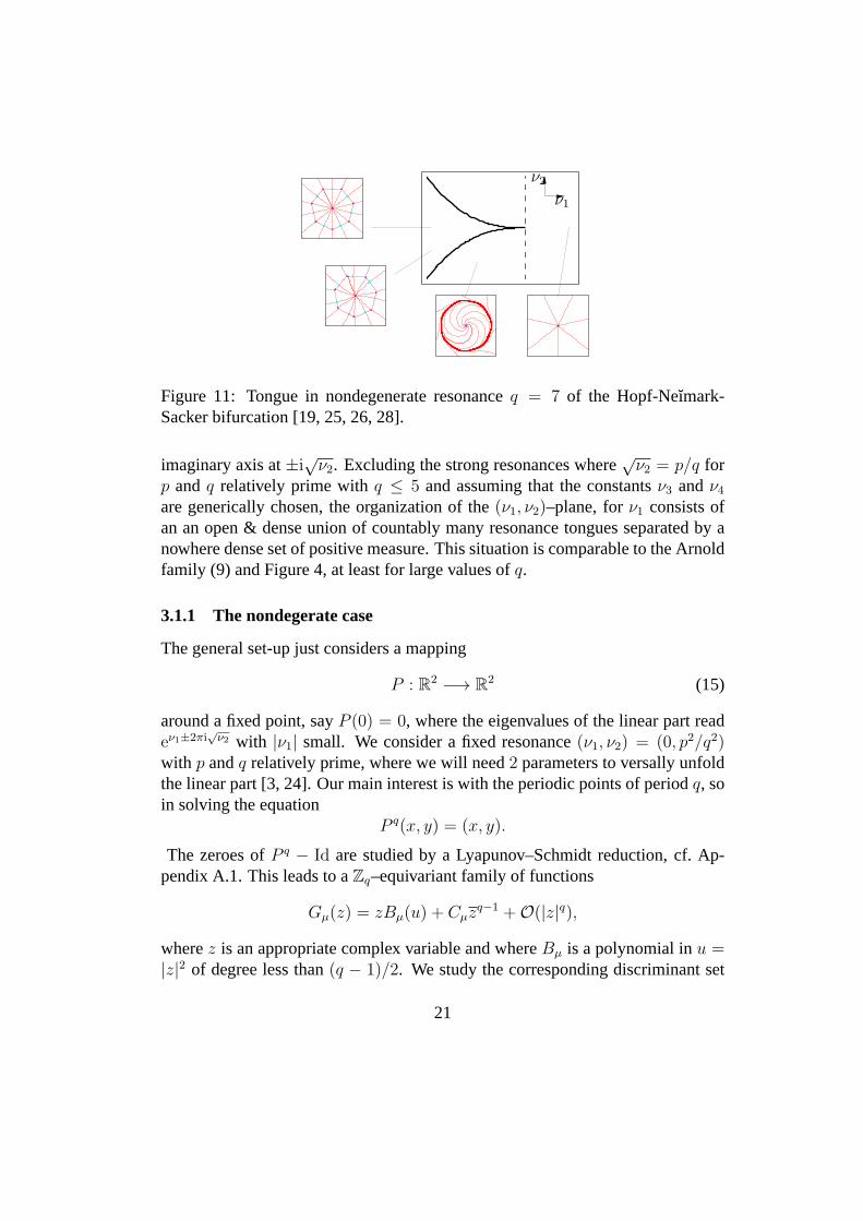
ν1

ν2

Figure 11: Tongue in nondegenerate resonanceq = 7 of the Hopf-Neımark-Sacker bifurcation [19, 25, 26, 28].

imaginary axis at±i√ν2. Excluding the strong resonances where

√ν2 = p/q for

p andq relatively prime withq ≤ 5 and assuming that the constantsν3 andν4are generically chosen, the organization of the(ν1, ν2)–plane, forν1 consists ofan an open & dense union of countably many resonance tongues separated by anowhere dense set of positive measure. This situation is comparable to the Arnoldfamily (9) and Figure 4, at least for large values ofq.

3.1.1 The nondegerate case

The general set-up just considers a mapping

P : R2 −→ R2 (15)

around a fixed point, sayP (0) = 0, where the eigenvalues of the linear part readeν1±2πi

√ν2 with |ν1| small. We consider a fixed resonance(ν1, ν2) = (0, p2/q2)

with p andq relatively prime, where we will need2 parameters to versally unfoldthe linear part [3, 24]. Our main interest is with the periodic points of periodq, soin solving the equation

P q(x, y) = (x, y).

The zeroes ofP q − Id are studied by a Lyapunov–Schmidt reduction, cf. Ap-pendix A.1. This leads to aZq–equivariant family of functions

Gµ(z) = zBµ(u) + Cµzq−1 +O(|z|q),

wherez is an appropriate complex variable and whereBµ is a polynomial inu =|z|2 of degree less than(q − 1)/2. We study the corresponding discriminant set

21

given byGµ(z) = 0 and detDzGµ(z) = 0. (16)

Hereµ is an unfolding-multiparameter detuning the resonance at hand. The wayto study this discriminant set is byZq–equivariant contact equivalence [19, 25, 26,27, 28]. In the present non-degenerate case (16) can be reduced to the polynomialnormal form

GNFσ (z) = z(σ + |z|2) + zq−1,

for a complex parameterσ. See also Appendix A.2, in particular Theorem 2. Ingeneral this set turns out to be a ‘tongue’ ending in a cusp of sharpness(q− 2)/2,which is part of a familiar bifurcation diagram with two periodic orbits of periodq inside that annihilate one another at the tongue boundariesin a saddle-node orfold bifurcation [3].

See Figure 11 which is embedded in the context of the equation(14), of whichPis a Poincare mapping. Here the dynamics ofP also has been described in termsof a Poincare–Takens interpolating normal form approximation, e.g., see [13, 44,45, 88] and Appendix A.3.

Globally a countable union of such cusps is separated by a nowhere dense setof positive measure, corresponding to invariant circles with Diophantine rotationnumber. As before, see Figure 4, the latter set contains the fractal geometry.

Remarks.

- The above results, summarized from [19, 25, 26, 28], are mainly obtainedbyZq–equivariant Singularity Theory.

- The strong resonances withq = 1, 2, 3 and4 form a completely differentstory where the Singularity Theory is far more involved [3, 88]. Still, sincethe higher order resonances accumulate at the boundaries, there is fractalgeometry around, always of positive measure.

- Regarding structural stability of unfoldings ofP as in (15) under topologicalconjugation, all hopes had already disappeared since [64].

22

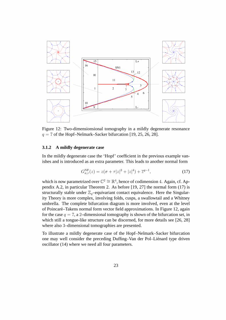
Figure 12: Two-dimensionsional tomography in a mildly degenerate resonanceq = 7 of the Hopf–Neımark–Sacker bifurcation [19, 25, 26, 28].

3.1.2 A mildly degenerate case

In the mildly degenerate case the ‘Hopf’ coefficient in the previous example van-ishes and is introduced as an extra parameter. This leads to another normal form

GNFσ,τ (z) = z(σ + τ |z|2 + |z|4) + zq−1, (17)

which is now parametrized overC2 ∼= R4, hence of codimension4. Again, cf. Ap-pendix A.2, in particular Theorem 2. As before [19, 27] the normal form (17) isstructurally stable underZq–equivariant contact equivalence. Here the Singular-ity Theory is more complex, involving folds, cusps, a swallowtail and a Whitneyumbrella. The complete bifurcation diagram is more involved, even at the levelof Poincare–Takens normal form vector field approximations. In Figure12, againfor the caseq = 7, a2–dimensional tomography is shown of the bifurcation set, inwhich still a tongue-like structure can be discerned, for more details see [26, 28]where also3–dimensional tomographies are presented.

To illustrate a mildly degenerate case of the Hopf–Neımark–Sacker bifurcationone may well consider the preceding Duffing–Van der Pol–Lienard type drivenoscillator (14) where we need all four parameters.

23

3.1.3 Concluding remarks

For both cases of the Hopf–Neımark–Sacker bifurcation we have a good grip onthe part of the bifurcation set that governs the number of periodic points. The fullbifurcation set is far more involved and the corresponding dynamics is describedonly at the level of Poincare–Takens normal-form vector fields [13, 26, 28]. Wenote that homo- and heteroclinic phenomena occur at a flat distance in terms ofthe bifurcation parameters [33, 41, 74].

3.2 The Hopf saddle-node bifurcation for diffeomorphisms

As a continuation of the above programme, we now consider theHopf saddle-node (or fold Hopf) bifurcation for diffeomorphisms [38, 39, 40], in which thecentral singularity is a fixed point of a3–dimensional diffeomorphism, such thatthe eigenvalues of the linear part at bifurcation are1 ande2πiα, where

e2πniα 6= 1 for n = 1, 2, 3 and 4,

so excluding strong resonances as in the Hopf–Neımark–Sacker case of§ 3.1. TheHopf saddle-node bifurcation for flows is well-known [43, 57], especially becauseof the subordinate Hopf–Neımark–Sacker andSilnikov homoclinic bifurcation.Our main interest is how the Hopf–Neımark–Sacker bifurcation is being changedinto one of the simplest quasi-periodic bifurcations near a2 : 5 resonance.

3.2.1 From vector fields to mappings

The linear part of the vector field at bifurcation has eigenvalues0 and±iα. Thislinear part generates an axial symmetry that in a normal formprocedure can bepushed stepwise over the entire Taylor series, see [13] and references. This makesit possible to first consider axially symmetric systems, that turn out to be topolog-ically determined by their3rd-order truncation given by

w = (−β2 + iα)w − awz − wz2

z = −β1 − sww − z2

wherew ∈ C andz ∈ R and whereβ1 andβ2 are unfolding parameters [57, 61].A scalingβ1 = γ2, β2 = γ2µ leads to a vector field

Yγ,µ,α(z, w) =

((−γµ+ 2πiα/γ)w − awz − γwz2

1− z2 − |w|2).

24

-0.1

-0.05

0

0.05

0.1

0.2 0.4 0.6 0.8 1 1.2 1.4O I

box H

H

-0.1

-0.05

0

0.05

0.1

0.2 0.4 0.6 0.8 1 1.2 1.4

δ

2π

δ

2π

µµ

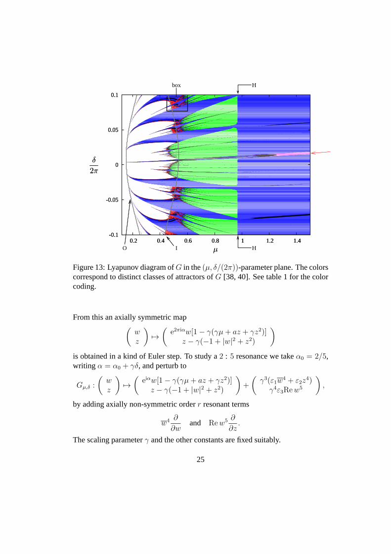
Figure 13: Lyapunov diagram ofG in the(µ, δ/(2π))-parameter plane. The colorscorrespond to distinct classes of attractors ofG [38, 40]. See table 1 for the colorcoding.

From this an axially symmetric map(

wz

)7→

(e2πiαw[1− γ(γµ+ az + γz2)]

z − γ(−1 + |w|2 + z2)

)

is obtained in a kind of Euler step. To study a2 : 5 resonance we takeα0 = 2/5,writing α = α0 + γδ, and perturb to

Gµ,δ :

(wz

)7→

(eiαw[1− γ(γµ+ az + γz2)]

z − γ(−1 + |w|2 + z2)

)+

(γ3(ε1w

4 + ε2z4)

γ4ε3Rew5

),

by adding axially non-symmetric orderr resonant terms

w4 ∂

∂wand Rew5 ∂

∂z.

The scaling parameterγ and the other constants are fixed suitably.

25

color Lyapunov exponents attractor type

red ℓ1 > 0 = ℓ2 > ℓ3 strange attractor

yellow ℓ1 > 0 > ℓ2 > ℓ3 strange attractor

blue ℓ1 = 0 > ℓ2 = ℓ3 invariant circle of focus type

green ℓ1 = ℓ2 = 0 > ℓ3 invariant 2-torus

black ℓ1 = 0 > ℓ2 > ℓ3 invariant circle of node type

grey 0 > ℓ1 > ℓ2 = ℓ3 fixed point of focus type

fuchsia 0 > ℓ1 = ℓ2 ≥ ℓ3 fixed point of focus type

pale blue 0 > ℓ1 > ℓ2 > ℓ3 fixed point of node type

white no attractor detected

Table 1: Legend of the color coding for Figure 13, see [38, 40]. The attractors areclassified by means of the Lyapunov exponents(ℓ1, ℓ2, ℓ3).

3.2.2 In the product of state space and parameter space

In Figure 13 a Lyapunov diagram is depicted in the parameter plane of the map-ping familyG. Table 1 contains the corresponding color code. In Figure 14weshow the dynamics corresponding to two values of(µ, δ/2π). Let us discuss thesenumerical data.

The parameter space. On the right-hand-side of the figure this method detectsan attracting invariant circle of focus type (blue). In the gaps larger resonancesare visible, compare with Figure 4 for a fixed value ofε. Moving to the left, in theneighbourhood of the line indicated by H a quasi-periodic Hopf bifurcation occursfrom a circle attractor to a2–torus attractor (green). Also here the parameterspace is interspersed with a resonance web of which the larger lines are visible.The remaining features, among other things, indicate invariant tori and strangeattractors of various types and also more invariant circles.

The state space. The upper two figures of Figure 14 show an invariant circle,once seen from thez–direction and once from somew–direction. The lower twofigures indicate how this circle has become a strange attractor, from the same twopoints of view.

26

-1

0

1

-1 0 1

Cn=0.46

x

y

-1

0

1

-1 0 1

C1

x

z

-1

0

1

-1 0 1

Dn=0.4555

x

y

-1

0

1

-1 0 1

D1

x

z

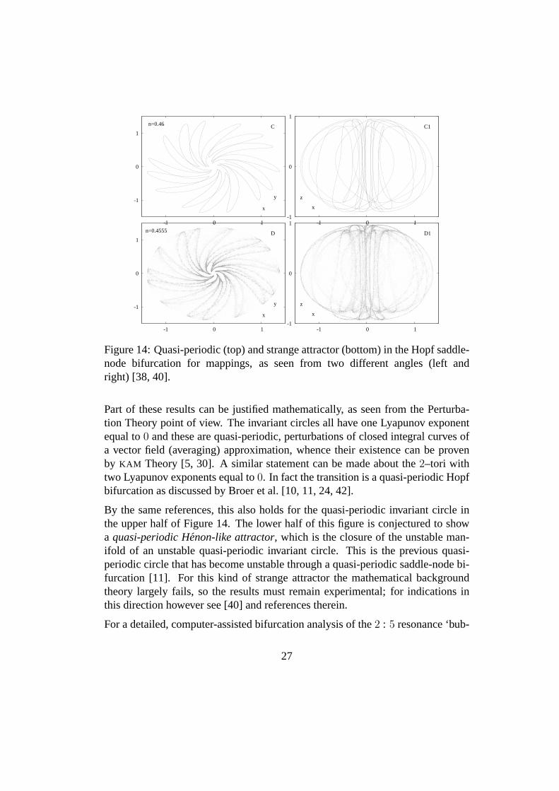
Figure 14: Quasi-periodic (top) and strange attractor (bottom) in the Hopf saddle-node bifurcation for mappings, as seen from two different angles (left andright) [38, 40].

Part of these results can be justified mathematically, as seen from the Perturba-tion Theory point of view. The invariant circles all have oneLyapunov exponentequal to0 and these are quasi-periodic, perturbations of closed integral curves ofa vector field (averaging) approximation, whence their existence can be provenby KAM Theory [5, 30]. A similar statement can be made about the2–tori withtwo Lyapunov exponents equal to0. In fact the transition is a quasi-periodic Hopfbifurcation as discussed by Broer et al. [10, 11, 24, 42].

By the same references, this also holds for the quasi-periodic invariant circle inthe upper half of Figure 14. The lower half of this figure is conjectured to showa quasi-periodic Henon-like attractor, which is the closure of the unstable man-ifold of an unstable quasi-periodic invariant circle. Thisis the previous quasi-periodic circle that has become unstable through a quasi-periodic saddle-node bi-furcation [11]. For this kind of strange attractor the mathematical backgroundtheory largely fails, so the results must remain experimental; for indications inthis direction however see [40] and references therein.

For a detailed, computer-assisted bifurcation analysis ofthe2 : 5 resonance ‘bub-

27

ble’ we refer to [38]. Compare with earlier work of Chenciner [46, 47, 48].We like to note that the family of mappingsG forms a concrete model for theRuelle–Takens scenario regarding the onset of turbulence. In fact it also illus-trates how the earlier scenario of Hopf–Landau–Lifschitz is also included: thepresent multi-parameter set-up unifies both approaches. For details and back-ground see [24, 42, 58, 59, 62, 63, 65, 79].

Resonance and fractal geometry. Interestingly, the blue colors right and leftcorrespond to quasi-periodic circle attractors. The fact that the correspondingregions of the plane look like open sets is misleading. In reality these are meagresets, dense veined by the residual sets associated to periodicity. These details arejust too fine to be detected by the computational precision used.

Particularly in the latter case, in the left half of the diagram, we are dealing withthe Arnold resonance web, for a detailed analysis see [39].

4 Conclusions

We discuss a number of consequences of the present paper in terms of modellingof increasing complexity.

4.1 ‘Next cases’

The Hopf saddle-node bifurcation for maps, see§ 3.2, can be viewed as a ‘nextcase’ in the systematic study of bifurcations as compared to, e.g., [57, 61] andmany others. The nowhere dense part of parameter space, since it lacks interiorpoints is somewhat problematic to penetrate by numerical continuation methods.Nevertheless, from the ‘physical’ point of view, this part surely is visible whenits measure is positive or, as in the present examples, even close to full measure.Needless to say that this observation already holds for the Hopf–Neımark–Sackerbifurcation as described in§ 3.1.

Other ‘next cases’ are formed by the quasi-periodic bifurcations which is a jointapplication of Kolmogorov–Arnold–Moser Theory [5, 11, 24,29, 42] and Singu-larity Theory [54, 55, 56, 89]. For overviews see [12, 49, 91]. The quasi-periodicbifurcations are inspired by the classical ones in which equilibria or periodic or-bits are replaced by quasi-periodic tori. As an example, in the Hopf saddle nodeof § 3.2 we met quasi-periodic Hopf bifurcation for mappings from circles to a

28

2–tori in a subordinate way. Here we witness a global geometryinspired by theclassical Hopf bifurcation, which concerns the quasi-periodic dynamics associ-ated to the fractal geometry in the parameter space, comparewith Figure 13. Thegaps or tongues in between concern the resonances inside, within which we noticea further ‘fractalization’ or ‘Cantorization’.

A similar ‘next case’ in complexity is given by the parametrically forced Lagrangetop [21, 29], in which a quasi-periodic Hamiltonian Hopf bifurcation occurs. In-deed, we recall from [51] that in the Lagrange top a Hamiltonian Hopf bifurcationoccurs, the geometry of which involves a swallowtail catastrophy. By the peri-odic forcing this geometry is ‘Cantorized’ yielding countably many tongues withfractal geometry in between.

Remarks.

- As said before, in cases with infinite regress the fractal complement is ameagre set which has positive measure. Simon [82] describesa similarsituation for1–dimensional Schrodinger operators. Also see [6].

- It is an interesting property of the real numbers to allow for this kind of di-chotomy in measure and topology, compare with Oxtoby [72]. Interestingly,although these properties in the first half of the 20th century were investi-gated for theoretical reasons, they here naturally show up in the context ofresonances and spectra.

4.2 Modelling

We like to note that our investigations on the Hopf saddle-node bifurcation formappings were inspired by climate models [16, 37, 85], wherein about 80–dimensional Galerkin projections of PDE models such bifurcations were detectedin 3–dimensional center manifolds.

Generally speaking there exists a large-scale programme ofmodelling in terms ofdynamical systems depending on parameters, with applications varying from cli-mate research to mathematical physics and biological cell systems. These modelsoften are high-dimensional and their complexity is partly explained by mecha-nisms of the present paper, also see [42, 79, 91]. In general such models exhibitthe coexistence of periodicity (including resonance), quasi-periodicity and chaos,best observed in the product of state- and parameter space.

29

Acknowledgements

The author thanks Konstantinos Efstathiou, Aernout van Enter and Ferdinand Ver-hulst for their help in the preparation of this paper.

References

[1] V.I. Arnol’d, Small divisors I: On mappings of the circleonto itself.Amer-ican Mathemathical Society Translations, Ser.246 (1965) 213-284

[2] V.I. Arnold, Mathematical Methods of Classical Mechanics.GTM 60Springer 1978

[3] V.I. Arnold, Geometrical Methods in the Theory of Ordinary DifferentialEquations.Springer 1983

[4] V.I. Arnold and A. Avez,Probemes Ergodiques de la Mecanique classique.Gauthier-Villars 1967;Ergodic problems of classical mechanics.Benjamin1968.

[5] V.I. Arnol’d, V.V. Kozlov and A.I. Neishtadt, Mathematical Aspects ofClassical and Celestial Mechanics. In: V.I. Arnol’d (ed.)Dynamical Sys-tems III.Springer 1988.

[6] A. Avila and D. Damanik, Generic singular spectrum for ergodicSchrodinger operators.Duke Math. J.130(2) (2005) 393-400

[7] C. Baesens, J. Guckenheimer, S. Kim and R.S. MacKay, Three coupledoscillators: Mode-locking, global bifurcation and toroidal chaos.PhysicaD 49(3) (1991) 387-475

[8] D.G.M. Beersma, H.W. Broer, K.A. Cargar, K. Efstathiou and I. Hoveijn,Pacer cell response to periodic Zeitgebers. Preprint University of Gronin-gen, 2011.

[9] M. Bennett, M.F. Schatz, H. Rockwood and K. Wiesenfeld, Huygensclocks.Proc. R. Soc. Lond.A 458(2002) 563-579

[10] B.L.J. Braaksma and H.W. Broer, On a quasi-periodic Hopf bifurcation.Annales Insitut Henri Poincare, Analyse non lineaire4 (1987) 115-168

30

[11] B.L.J. Braaksma, H.W. Broer and G.B. Huitema, Towards a quasi-periodicbifurcation theory.Mem. AMS83(421) (1990), 81175

[12] H.W. Broer, KAM theory: the legacy of Kolmogorov’s 1954 paper.Bull.AMS (New Series)41(4) (2004) 507-521

[13] H.W. Broer, Normal forms in perturbation theory. In: R. Meyers (ed.),En-cyclopædia of Complexity & System Science. Springer (2009) 6310-6329

[14] H.W. Broer, M.C. Ciocci, H. Hanßmann and A. Vanderbauwhede, Quasi-periodic stability of normally resonant tori.Physica D(2009) 309318

[15] H.W. Broer, B. Hasselblatt and F. Takens (eds.):Handbook of DynamicalSystemsVolume3 North-Holland 2010.

[16] H.W. Broer, H.A. Dijkstra, C. Simo, A.E. Sterk and R. Vitolo, The dynam-ics of a low-order model for the Atlantic Multidecadal Oscillation.DCDS-B16(1) (2011) 73102

[17] H.W. Broer, K. Efstathiou, and E. Subramanian, Robustness of unstable at-tractors in arbitrarily sized pulse-coupled systems with delay.Nonlinearity21 (2008) 1349

[18] H.W. Broer, K. Efstathiou, and E. Subramanian, Heteroclinic cycles be-tween unstable attractors.Nonlinearity21 (2008) 13851410

[19] H.W. Broer, M. Golubitsky and G. Vegter, The geometry of resonancetongues: A Singularity Theory approach.Nonlinearity 16 (2003) 1511-1538

[20] H.W. Broer, M. Golubitsky, and G. Vegter. Geometry of resonance tongues.Singularity Theory. Proceedings of the 2005 Marseille Singularity Schooland Conference, pages 327–356, 2007.

[21] H.W. Broer, H. Hanßmann and J. Hoo, The quasi-periodic HamiltonianHopf bifurcation.Nonlinearity20 (2007) 417-460

[22] H.W. Broer, H. Hanßmann,A. Jorba, J. Villanueva and F.O.O. Wagener,Normal-internal resonances in quasi-periodically forcesoscillators: a con-servative approach.Nonlinearity16 (2003) 1751-1791

31

[23] H.W. Broer, H. Hanßmann and J. You, On the destruction of resonant La-grangean tori in Hamiltonian systems. Preprint Universiteit Utrecht (2008)

[24] H.W. Broer, H. Hanßmann and F.O.O. Wagener,Quasi-periodic bifurcationtheory: the geometry ofKAM . 2012 (to appear)

[25] H.W. Broer, S.J. Holtman and G. Vegter, Recognition of thebifurcationtype of resonance in a mildly degenerate Hopf-Neımark-Sacker families.Nonlinearity21 (2008) 2463-2482

[26] H.W. Broer, S.J. Holtman, G. Vegter and R. Vitolo, Geometry and dynam-ics of mildly degenerate Hopf-Neımarck-Sacker families near resonance.Nonlinearity22 (2009) 2161-2200

[27] H.W. Broer, S.J. Holtman and G. Vegter, Recognition of resonance type inperiodically forced oscillators.Physica-D239(17) (2010) 1627-1636

[28] H.W. Broer, S.J. Holtman, G. Vegter and R. Vitolo, Dynamics and Geom-etry Near Resonant Bifurcations.Regular and Chaotic Dynamics16(1-2)(2011) 3950

[29] H.W. Broer, J. Hoo and V. Naudot, Normal linear stabilityof quasi-periodictori. J. Differential Equations232(2007) 355-418

[30] H.W. Broer, G.B. Huitema and F. Takens, Unfoldings and bifurcationsof quasi-periodic tori.Memoirs American Mathematical Society83 # 421(1990) 1-82

[31] H.W. Broer and M. Levi, Geometrical aspects of stabilitytheory for Hill’sequations.Archive Rat. Mech. An.131(1995) 225-240

[32] H.W. Broer, J. Puig and C. Simo, Resonance tongues and instability pocketsin the quasi-periodic Hill-Schrodinger equation.Commun. Math. Phys.241(2003) 467-503

[33] H.W. Broer and R. Roussarie, Exponential confinement of chaos inthe bifurcations sets of real analytic diffeomorphisms. In: H.W. Broer,B. Krauskopf and G. Vegter (eds.)Global Analysis of Dynamical Systems.IoP Publishing (2001) 167-210

32

[34] H.W. Broer and C. Simo, Hill’s equation with quasi-periodic forcing: res-onance tongues, instability pockets and global phenomena.Boletim So-ciedade Brasileira Matematica29 (1998) 253-293

[35] H.W. Broer and C. Simo, Resonance tongues in Hill’s equations: a geomet-ric approach.Journal of Differential Equations166(2000) 290-327

[36] H.W. Broer, C. Simo and J.C. Tatjer, Towards global models near homo-clinic tangencies of dissipative diffeomorphisms.Nonlinearity11(3) (1998)667-770

[37] H.W. Broer, C. Simo and R. Vitolo, Bifurcations and strange attractorsin the Lorenz-84 climate model with seasonal forcing.Nonlinearity15(4)(2002) 1205-1267

[38] H.W. Broer, C. Simo and R. Vitolo, The Hopf-Saddle-Node bifurcationfor fixed points of 3D-diffeomorphisms, analysis of a resonance ‘bubble’.Physica D237(2008) 1773-1799

[39] H.W. Broer, C. Simo and R. Vitolo, The Hopf-Saddle-Node bifurcationfor fixed points of 3D-diffeomorphisms, the Arnol′d resonance web.Bull.Belgian Math. Soc. Simon Stevin15 (2008) 769-787

[40] H.W. Broer, C. Simo and R. Vitolo, Chaos and quasi-periodicity in diffeo-morphisms of the solid torus.DCDS-B14(3) (2010) 871-905

[41] H.W. Broer and F. Takens, Formally symmetric normal forms and generic-ity. Dynamics Reported2 (1989) 36-60

[42] H.W. Broer and F. Takens,Dynamical Systems and Chaos.Appl. Math. Sc.172Springer 2011

[43] H.W. Broer and G. Vegter, Subordinate Sil’nikov bifurcations near somesingularities of vector fields having low codimension.Ergodic Theory Dy-namical Systems4 (1984) 509-525

[44] H.W. Broer and G. Vegter, Bifurcational aspects of parametric resonance.Dynamics Reported, New Series1 (1992) 1-51

[45] H.W. Broer and G. Vegter, Generic Hopf-Neımark-Sacker bifurcations infeed forward systems.Nonlinearity21 (2008) 1547-1578

33

[46] A. Chenciner, Bifurcations de points fixes elliptiques. I. Courbes invari-antes.Publ. Math. IHES61 (1985) 67-127

[47] A. Chenciner, Bifurcations de points fixes elliptiques. II. Orbitesperiodiques et ensembles de Cantor invariants.Invent. Math.80 (1985) 81-106

[48] A. Chenciner, Bifurcations de points fixes elliptiques. III. Orbitesperiodiques de “petites” periodes etelimination resonnante des couples decourbes invariantes.Publ. Math. IHES66 (1988) 5-91

[49] M.C. Ciocci, A. Litvak-Hinenzon and H.W. Broer, Survey on dissipativeKAM theory including quasi-periodic bifurcation theory basedon lecturesby Henk Broer. In: J. Montaldi and T. Ratiu (Eds.):Geometric Mechan-ics and Symmetry: the Peyresq Lectures.LMS Lecture Notes Series,306Cambridge University Press (2005) 303-355

[50] A. Correia and J. Laskar, Mercury’s capture into the 3/2 spin-orbit reso-nance as a result of its chaotic dynamics.Nature429(2004) 848-850

[51] R.H. Cushman and J.C. van der Meer, The Hamiltonian Hopf bifurca-tion in the Lagrange top. In: C. Albert (ed.)Geometrie Symplectique etMechanique, Colloque International La Grande Motte, France,23-28Mai,1988. Lecture Notes in Mathematics1416(1990) 26-38

[52] R.L. Devaney,An Introduction to Chaotic Dynamical Systems. 2nd Edition.Addison-Wesley 1989

[53] L.H. Eliasson, Floquet solutions for the one-dimensional quasi-periodicSchrodinger equation.Commun. Math. Phys.146(1992) 447-482

[54] M. Golubitsky and V. Guillemin,Stable Mappings and Their Singularities.Springer (1973)

[55] M. Golubitsky and D.G. Schaeffer,Singularities and Groups in BifurcationTheoryVol. I. Springer (1985)

[56] M. Golubitsky, I. Stewart and D.G. Schaeffer,Singularities and Groups inBifurcation TheoryVol. II. Appl. Math. Sc.69Springer (1988)

34

[57] J. Guckenheimer and P. Holmes,Nonlinear Oscillations, Dynamical Sys-tems, and Bifurcations of Vector Fields, Fifth Edition. Applied Mathemati-cal Sciences42, Springer 1997

[58] E. Hopf, A Mathematical Example Displaying Features ofTurbulence.Comm. (Pure) Applied Mathematics1 (1948) 303-322

[59] E. Hopf, Repeated branching through loss of stability, an example. In:J.B. Diaz (ed.)Proceedings of the conference on differential equations,Maryland1955. University Maryland book store (1956) 49-56

[60] C. Huygens,Œvres completes de Christiaan Huygens.(1888-1950) Vol. 5,241-263 and Vol. 17, 156-189. Martinus Nijhoff 1888-1950

[61] Yu.A. Kuznetsov,Elements of Applied Bifurcation Theory, Third Edition.Applied Mathematical Sciences112, Springer 2004

[62] L.D. Landau, On the problem of turbulence.Doklady Akademii Nauk SSSR44 (1944) 339-342

[63] L.D. Landau and E.M. Lifshitz,Fluid Mechanics, Second Edition. Perga-mon (1987)

[64] S.E. Newhouse, J. Palis and F. Takens, Bifurcations and stability of familiesof diffeomorphisms.Publ. Math. IHES57 (1983) 5-71

[65] S.E. Newhouse, D. Ruelle and F. Takens, Occurrence of strange Axiom Aattractors near quasi-periodic flows onTm, m ≤ 3. Commun. Math. Phys.64 (1978) 35-40

[66] B.B. Mandelbrot,The Fractal Geometry of Nature.Freeman (1977).

[67] J.K. Moser, On invariant curves of area-preserving mappings of an annulus.Nachrichten Akademie Wissenschaften Gottingen, Mathematisch–Physika-lische Klasse II.1 (1962) 1-20

[68] J.K. Moser, Lectures on Hamiltonian systems.Memoirs American Mathe-matical Society81 (1968) 1-60

[69] J.K. Moser, Stable and random motions in dynamical systems, with specialemphasis to celestial mechanics,Annals Mathematical Studies77 (1973)Princeton University Press.

35

[70] J.K. Moser and J. Poschel, An extension of a result by Dinaburg and Sinaion quasi-periodic potentials.Comment. Math. Helvetici59 (1984) 39-85

[71] Z. Nitecki, Differentiable dynamics. An introduction to the orbit structureof diffeomorphisms.Massachusetts Institute of Technology Press 1971.

[72] J. Oxtoby,Measure and Category.Springer 1971

[73] J. Palis, W.C. de Melo,Geometric Theory of Dynamical Systems.Springer1982

[74] J. Palis and F. Takens,Hyperbolicity & sensitive chaotic dynamics at ho-moclinic bifurcations.Cambridge University Press (1993)

[75] J.H. Poincare, Les Methodes Nouvelles de la Mecanique CelesteI, II, III .Gauthier-Villars (1892, 1893, 1899). Republished by Blanchard (1987).

[76] A. Pogromsky, D. Rijlaarsdam and H. Nijmeijer, Experimental Huygenssynchronization of oscillators. In: M. Thiel, J. Kurths, M.C. Romano,A. Moura and G. Karolyi, Nonlinear Dynamics and Chaos: Advances andPerspectives.Springer Complexity (2010) 195-210

[77] B. van der Pol, De amplitude van vrije en gedwongen triode-trillingen. Ti-jdschrift Nederlands Radiogenooschap1 (1920) 3-31

[78] B. van der Pol, The nonlinear theory of electric oscillations.ProceedingsInstitute Radio England22 (1934) 1051-1086; Reprinted in:Selected Sci-entific Papers.North-Holland 1960

[79] D. Ruelle and F. Takens, On the nature of turbulence.Comm. Math. Phys.20 (1971) 167-192;23 (1971) 343-344

[80] J.A. Sanders, F. Verhulst and J. Murdock,Averaging Methods in Nonlin-ear Dynamical Systems, Revised Second Edition. Applied MathematicalSciences59, Springer (2007)

[81] C.L. Siegel and J.K. Moser,Lectures on Celestial Mechanics.Springer(1971)

[82] B. Simon, Operators with singular continuous spectrum:I. General opera-tors.Ann. of Math.141(1995) 131-145

36

[83] W. de Sitter, On the libration of the three inner large satellites of Jupiter.Publ. Astr. Lab. Groningen17 (1907) 1-119

[84] W. de Sitter, New mathematical theory of Jupiters satellites. Ann. Ster-rewacht LeidenXII (1925)

[85] A.E. Sterk, R. Vitolo, H.W. Broer, C. Simo and H.A. Dijkstra, New non-linear mechanisms of midlatitude atmospheric low-frequency variability.Physica D239(10) (2010) 702718

[86] J.J. Stoker,Nonlinear Vibrations in Mechanical and Electrical Systems.2nd Ed.Wiley 1992

[87] S.H.Strogatz,Nonlinear Dynamics and Chaos.Addison Wesley 1994

[88] F. Takens, Forced oscillations and bifurcations. In: Applications of GlobalAnalysis I,Comm. of the Math. Inst. Rijksuniversiteit Utrecht(1974). In:H.W. Broer, B. Krauskopf and G. Vegter (Eds.),Global Analysis of Dynam-ical SystemsIoP Publishing (2001) 1-62

[89] R. Thom,Stabilite Structurelle et Morphogenese.Benjamin 1972

[90] F. Verhulst,Nonlinear Differential Equations and Dynamical Systems. 2ndEdition.Universitext Springer 1996

[91] R. Vitolo, H.W. Broer, and C. Simo, Quasi-periodic bifurcations of invari-ant circles in low-dimensional dissipative dynamical systems.Regular andChaotic Dynamics16(1-2) (2011) 154184

[92] A. Vanderbauwhede. Branching of periodic solutions in time-reversiblesystems. In H.W. Broer and F. Takens, editors,Geometry and Analysis inNon-Linear Dynamics, volume 222 ofPitman Research Notes in Mathe-matics, pages 97–113. Pitman, London, 1992.

[93] A. Vanderbauwhede. Subharmonic bifurcation at multiple resonances. InProceedings of the Mathematics Conference, pages 254–276, Singapore,2000. World Scientific.

37

A Equivariant Singularity Theory

A.1 Lyapunov–Schmidt reduction

Our method for finding resonance tongues — and tongue boundaries — proceedsas follows. Find the region in parameter space corresponding to points wherethe mapP has aq-periodic orbit; that is, solve the equationP q(x) = x. Usinga method due to Vanderbauwhede (see [92, 93]), we can solve for such orbitsby Lyapunov-Schmidt reduction. More precisely, aq-periodic orbit consists ofqpointsx1, . . . , xq where

P (x1) = x2, . . . , P (xq−1) = xq, P (xq) = x1.

Such periodic trajectories are just zeroes of the map

P (x1, . . . , xq) = (P (x1)− x2, . . . , P (xq)− x1).

Note thatP (0) = 0, and that we can find all zeroes ofP near the resonance pointby solving the equationP (x) = 0 by Lyapunov-Schmidt reduction. Note also thatthe mapP hasZq symmetry. More precisely, define

σ(x1, . . . , xq) = (x2, . . . , xq, x1).

Then observe thatP σ = σP .

At 0, the Jacobian matrix ofP has the block form

J =

A −I 0 0 · · · 0 00 A −I 0 · · · 0 0

...0 0 0 0 · · · A −I

−I 0 0 0 · · · 0 A

whereA = (dP )0. The matrixJ automatically commutes with the symmetryσ and henceJ can be block diagonalized using the isotypic components of ir-reducible representations ofZq. (An isotypic componentis the sum of theZq

isomorphic representations. See [56] for details. In this instance all calculations

38

can be done explicitly and in a straightforward manner.) Over the complex num-bers it is possible to write these irreducible representations explicitly. Letω be aqth root of unity. DefineVω to be the subspace consisting of vectors

[x]ω =

xωx

...ωq−1x

.

A short calculation shows that

J [x]ω = [(A− ωI)x]ω.

ThusJ has zero eigenvalues precisely whenA hasqth roots of unity as eigenval-ues. By assumption,A has just one such pair of complex conjugateqth roots ofunity as eigenvalues.

Since the kernel ofJ is two-dimensional — by the simple eigenvalue assump-tion in the Hopf bifurcation — it follows using Lyapunov-Schmidt reduction thatsolving the equationP (x) = 0 near a resonance point is equivalent to findingthe zeros of a reduced map fromR2 → R2. We can, however, naturally identifyR2 with C, which we do. Thus we need to find the zeros of a smooth implicitlydefined function

g : C → C,

whereg(0) = 0 and(dg)0 = 0. Moreover, assuming that the Lyapunov-Schmidtreduction is done to respect symmetry, the reduced mapg commutes with theaction ofσ on the critical eigenspace. More precisely, letω be the critical resonanteigenvalue of(dP )0; then

g(ωz) = ωg(z). (18)

Sincep andq are coprime,ω generates the groupZq consisting of allqth roots ofunity. Sog is Zq-equivariant.

We propose to useZq-equivariant singularity theory to classify resonancetongues and tongue boundaries.

A.2 Equivariant Singularity Theory

In this section we develop normal forms for the simplest singularities of Zq-equivariant mapsg of the form (18), as presented in Section 3.1. To do this,we need to describe the form ofZq-equivariant maps, contact equivalence, andfinally the normal forms.

39

The structure of Zq-equivariant maps. We begin by determining a uniqueform for the generalZq-equivariant polynomial mapping. By Schwarz’s theorem[56] this representation is also valid forC∞ germs.

Lemma 1. EveryZq-equivariant polynomial mapg : C → C has the form

g(z) = K(u, v)z + L(u, v)zq−1,

whereu = zz, v = zq + zq, and K,L are uniquely defined complex-valuedfunction germs.

Zq contact equivalences. Singularity theory approaches the study of zeros ofa mapping near a singularity by implementing coordinate changes that transformthe mapping to a ‘simple’ normal form and then solving the normal form equa-tion. The kinds of transformations that preserve the zeros of a mapping are calledcontact equivalences. More precisely, twoZq-equivariant germsg andh areZq-contact equivalentif

h(z) = S(z)g(Z(z)),

whereZ(z) is aZq-equivariant change of coordinates andS(z) : C → C is a reallinear map for eachz that satisfies

S(γz)γ = γS(z)

for all γ ∈ Zq.

Normal form theorems. In this section we consider two classes of normalforms — the codimension two standard for resonant Hopf bifurcation and onemore degenerate singularity that has a degeneracy at cubic order. These singu-larities all satisfy the nondegeneracy conditionL(0, 0) 6= 0; we explore this casefirst.

Theorem 2. Suppose that

h(z) = K(u, v)z + L(u, v)zq−1

whereK(0, 0) = 0.

1. Letq ≥ 5. If KuL(0, 0) 6= 0, thenh is Zq contact equivalent to

g(z) = |z|2z + zq−1

with universal unfolding

G(z, σ) = (σ + |z|2)z + zq−1.

40

2. Letq ≥ 7. If Ku(0, 0) = 0 andKuu(0, 0)L(0, 0) 6= 0, thenh is Zq contactequivalent to

g(z) = |z|4z + zq−1

with universal unfolding

G(z, σ, τ) = (σ + τ |z|2 + |z|4)z + zq−1,

whereσ, τ ∈ C.

Remark. Normal forms for the casesq = 3 and q = 4 are slightly different.See [19] for details.

A.3 Resonances in forced oscillators

As indicated in Section 2.1 subharmonic bifurcations in periodicially forced os-cillators and the can be studied by lifting the system to a suitable covering space.This section contains the details of this procedure.

Hopf-Neımark-Sacker bifurcations in forced oscillators. Forced oscillatorsdepending on parameters may undergo bifurcations involving the birth or death ofsubharmonics. In particular, we consider2π-periodic systems onC of the form

z = F (z, z, µ) + εG(z, z, t, µ), (19)

obtained from an autonomous system by a small2π-periodic perturbation. Hereε is a real perturbation parameter, andµ ∈ Rk is an additionalk-dimensionalparameter. Subharmonics of orderq may appear or disappear upon variation ofthe parameters if the linear part ofF atz = 0 satisfies ap : q-resonance conditionwhich is appropriately detuned upon variation of the parameterµ.

The Hopf-Neımark-Sacker Normal form of such systems reveals this type ofbifurcation. To this end, consider a2π-periodic forced oscillator onC of the form

z = X(z, z, t, µ),

where

X(z, z, t, µ) = iωNz + (α + iδ)z + zP (z, z, µ) + εQ(z, z, t, µ). (20)

Hereµ ∈ Rk, andε is a small real parameter. Furthermore we assume thatPandQ contain no terms that are independent ofz andz (i.e.,P (0, 0, µ) = 0 and

41

Q(0, 0, t, µ) = 0), and thatQ does not even contain terms that are linear inzandz. Any system of the form (19) with linear partz = iωNz can be broughtinto this form after a straightforward initial transformation. See [30, Part II] fordetails. Applying the algorithm of, e.g., [20], this systemcan be brought into thefollowing Hopf-Neımark-Sacker normal form:

Theorem 3. (Normal Form to order q)The system (20) has normal form

z = iωNz + (α + iδ)z + zF (|z|2, µ) + d ε zq−1 eipt +O(q + 1), (21)

whereF (|z|2, µ) is a complex polynomial of degreeq − 1 with F (0, µ) = 0, andd is a complex constant.

Subharmonics of orderq are to be expected if the linear part satisfies ap : q-

resonance condition, in other words, if the normal frequency ωN is equal top

q(with p andq relatively prime). To explore these subharmonics further we applythe Van der Pol transformation and bring the Poincare-map of the lifted systeminto its Takens Normal Form.

Existence of2πq-periodic orbits. The Van der Pol transformation. Sub-harmonics of orderq of the 2π-periodic forced oscillator (20) correspond toq-periodic orbits of the Poincare time2π-mapP : C → C. These periodic orbitsof the Poincare map are brought into one-one correspondence with the zerosofa vector field on aq-sheeted cover of the phase spaceC × R/(2πZ) via theVander Pol transformation, cf [44]. This transformation corresponds to aq-sheetedcovering

Π : C× R/(2πqZ) → C× R/(2πZ),

(z, t) 7→ (zeitp/q, t (mod2πZ)) (22)

with cyclic Deck group of orderq generated by

(z, t) 7→ (ze2πip/q, t− 2π).

The Van der Pol transformationζ = ze−iωN t lifts the forced oscillator (19) to thesystem

ζ = (α + iδ)ζ + ζP (ζeiωN t, ζe−iωN t, µ) + εQ(ζeiωN t, ζe−iωN t, t, µ) (23)

42

on the covering spaceC × R/(2πqZ). The latter system isZq-equivariant. Astraightforward application of (23) to the normal form (21)yields the followingnormal form for the lifted forced oscillator.

Theorem 4. (Equivariant Normal Form of order q)On the covering space, the lifted forced oscillator has theZq-equivariant normalform:

ζ = (α + iδ)ζ + ζF (|ζ|2, µ) + d ε ζq−1

+O(q + 1), (24)

where theO(q + 1) terms are2πq-periodic.

Resonance tongues for families of forced oscillators.Bifurcations ofq-periodicorbits of the Poincare mapP on the base space correspond to bifurcations of fixedpoints of the Poincare mapP on theq-sheeted covering space introduced in con-nection with the Van der Pol transformation (22). Denoting the normal form sys-tem (21) on the base space byN , and the normal form system (24) of the liftedforced oscillator byN , we see that

Π∗N = N .

The Poincare mappingP of the normal form on the covering space now is the2πq-period mapping

P = N 2πq +O(q + 1),

whereN 2πq denotes the2πq-map of the (planar) vector fieldN . Following theCorollary to the Normal Form Theorem of [44, page 12], we conclude for theoriginal Poincare mapP of the vector fieldX on the base space that

P = R2πωN◦ N 2π +O(q + 1),

whereR2πωNis the rotation over2πωN = 2πp/q, which precisely is the Takens

Normal Form ofP at (z, µ) = (0, 0), see [88].Our interest is with theq-periodic points ofPµ, which correspond to the fixed

points ofPµ. This fixed point set and the boundary thereof in the parameterspaceR3 = {a, δ, ε} is approximately described by the discriminant set of

(a+ iδ)ζ + ζF (|ζ|2, µ) + εdζq−1

,

which is the truncated right hand side of (24). This gives rise to the bifurcationequation that determine the boundaries of the resonance tongues. The followingtheorem implies that, under the conditions thatd 6= 0 6= Fu(0, 0), the order oftangency at the tongue tips is generic. HereFu(0, 0) is the partial derivative ofF (u, µ) with respect tou.

43

Theorem 5. (Bifurcation equations modulo contact equivalence)Assume thatd 6= 0 andFu(0, 0) 6= 0. Then the polynomial (24) isZq-equivariantlycontact equivalent with the polynomial

G(ζ, µ) = (a+ iδ + |ζ|2)ζ + εζq−1

. (25)

The discriminant set of the polynomialG(ζ, µ) is of the form

δ = ±ε(−a)(q−2)/2 +O(ε2). (26)

Proof. The polynomial (25) is a universal unfolding of the germ|ζ|2ζ + εζq−1

underZq contact equivalence. See [19] for a detailed computation. The tongueboundaries of ap : q resonance are given by the bifurcation equations

G(ζ, µ) = 0,

det(dG)(ζ, µ) = 0.

As in [19, Theorem 3.1] we putu = |z|2, and b(u, µ) = a + iδ + u. ThenG(ζ, µ) = b(u, µ)ζ + εζ

q−1. According to (the proof of) [19, Theorem 3.1], the

system of bifurcation equations is equivalent to

|b|2 = ε2uq−2,

bb′+ bb′ = (q − 2)ε2uq−3,

whereb′ =∂b

∂u(u, µ). A short computation reduces the latter system to the equiv-

alent

(a+ u)2 + δ2 = ε2uq−2,

a+ u =1

2(q − 2)ε2uq−3.

Eliminatingu from this system of equations yields expression (26) for thetongueboundaries.

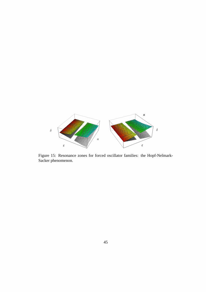
The discriminant set of the equivariant polynomial (25) forms the boundaryof the resonance tongues. See Figure 15. At this surface we expect the Hopf-Neımark-Sacker bifurcation to occur; here the Floquet exponents of the linear partof the forced oscillator cross the complex unit circle. Thisbifurcation gives rise toan invariant 2-torus in the 3D phase spaceC×R/(2πZ). Resonances occur whenthe eigenvalues cross the unit circle at roots of unitye2πip/q. ‘Inside’ the tonguethe 2-torus is phase-locked to subharmonic periodic solutions of orderq.

44

a

εε

δ

aa

εε

δ

Figure 15: Resonance zones for forced oscillator families: the Hopf-Neımark-Sacker phenomenon.

45