Singularities of eddy current problems

Martin Costabel, Monique Dauge, Serge Nicaise

May 13, 2003

AbstractWe consider the time-harmonic eddy current problem in its electric formulation where

the conductor is a polyhedral domain. By proving the convergence in energy, we justify inwhat sense this problem is the limit of a family of Maxwell transmission problems: Ratherthan a low frequency limit, this limit has to be understood in the sense of BOSSAVIT [11].We describe the singularities of the solutions. They are related to edge and corner singu-larities of certain problems for the scalar Laplace operator, namely the interior Neumannproblem, the exterior Dirichlet problem, and possibly, an interface problem. These singu-larities are the limit of the singularities of the related family of Maxwell problems.

Key Words Eddy current problem, corner singularity, edge singularity.AMS (MOS) subject classification 35B65, 35R05, 35Q60.

1 Maxwell equations and the eddy current limit

Let us consider the model case of an homogeneous conducting bodyΩC which we assume tobe a three-dimensional bounded polyhedral domain with a Lipschitz boundaryB. The conduc-tivity σ = σC is constant and positive insideΩC , while σ vanishes outsideΩC , i.e.,σ ≡ 0 inthe “air” (or “empty”) regionΩE = R

3 \ΩC . For the sake of simplicity we further assume thatthe boundaryB of ΩC is connected(∗). The electric permittivityε is equal to a positive con-stantεC insideΩC and has another valueεE in the exterior medium. Similarly, the magneticpermeabilityµ is equal toµC > 0 in ΩC and toµE > 0 in ΩE . The treatment of piecewiseconstantσC , εC , µC andµE can be made in a similar manner.

1.1 Maxwell and eddy current problems

Let ω > 0 be a fixed frequency. The time harmonic Maxwell equations are

curl E = −iωµH in R3,(1)

curl H = (iωε + σ)E + j0 in R3,(2)

E (resp.H) is the electric (resp. magnetic) field andj0 is the source current density which issupposed to be aL2(R3) field with support inΩC and to be divergence free, i.e.div j0 = 0 inR

3. Let us recall(∗)The issue of a multiple connectedB is independent of the question of singularities. We will just mention the

modifications necessary whenB is multiply connected, see Remark 3 at the end of§2.

1

Lemma 1.1 Let u ∈ L2(R3)3 be such that u|ΩE≡ 0 and div u = 0 in R

3. Then the normaltrace u|ΩC

·n on B is zero (here n denotes the unit outward normal vector on B, pointing fromΩC to ΩE).

Thus the assumption on div j0 is equivalent to

div j0 = 0 in ΩC and j0 · n = 0 on B.

Note that, taking the divergence of equation (2), we obtain the following equation on thedivergence of E:

div(iωε + σ)E = 0 in R3.(3)

Equations (1) – (2) have to be completed by conditions at infinity (Silver-Muller radiationconditions)

lim|x|→∞

(H× x− |x|E

)= 0.(4)

The time-harmonic eddy current problem [10, 11, 3, 22] reads

curl E = −iωµH in R3,(5)

curl H = σE + j0 in R3.(6)

Let us denote E|ΩCand E|ΩE

by EC and EE , respectively. Now, taking the divergence ofequation (6) we only obtain, thanks to Lemma 1.1, div EC = 0 in ΩC and EC · n = 0 on B.These conditions have to be completed by the gauge conditions:

div EE = 0 in ΩE and∫B

EE · n dS = 0.(7)

The condition at infinity takes the form

E(x) = O(|x|−1), H(x) = O(|x|−1) as |x| → ∞.(8)

Remark 1 The equations (5)-(6) are clearly obtained from (1)-(2) by setting ε to zero. Thegauge conditions (7) can also be obtained from (3): Since iωε+ σ is equal to the two non-zeroconstants iωεC + σ in ΩC and iωεE in ΩE , (3) implies that div EC = 0 in ΩC , div EE = 0 inΩE and (by a result similar to Lemma 1.1)

(iωεC + σC)EC · n = iωεEEE · n on B.(9)

The condition div EC = 0 implies by integration by parts that∫B EC ·n = 0. Then, by (9), we

obtain that ∫B

EE · n dS = 0.(10)

Setting εC = εE = 0, we obtain (7) and the two conditions issued from the equation div(σE) =0, that is

div E = 0 in ΩC ∪ ΩE and EC · n = 0 on B.(11)

2

Thus we see that the gauge conditions (7) are natural. But we obtain them by first deducingconditions on the divergence of the Maxwell solution E and then passing to the limit. Theconverse order does not provide (7).

Remark 2 The conditions at infinity (4) imply the uniqueness of solutions for equations (1)-(2) (Rellich lemma). Moreover, with the (exterior) wave number k := ω

√εEµE , we have the

following asymptotics at infinity (here x := x/|x|):

E(x) =eik|x|

|x|(

E∞(x) + O(|x|−1))

as |x| → ∞.

The function E∞ is the electric far field pattern, see [12].Concerning equations (5)-(7), the conditions at infinity (8) also imply the uniqueness, and thefollowing asymptotics at infinity holds [3, Prop.3.1]

E(x) = O(|x|−2), H(x) = O(|x|−2) as |x| → ∞.

This means that the far field pattern goes to zero in the eddy current limit.

1.2 Eddy current limit

We want to give a sense to the notion of eddy current limit: This means that the quantitiesωεC/σC and ωεE/σC are small. For a conducting material, the permittivity εC is of the sameorder of magnitude than εE (also denoted ε0), but εC/σC is very small. For moderate frequen-cies ω the quantities ωεC/σC and ωεE/σC are still small. Let us fix two numbers εC and εEwhich are of the same order than σC and such that there exists δ > 0 (thus δ is small)

εC = δεC and εE = δεE .(12)

Thus

iωε + σ =

iωδεC + σC in ΩC

iωδεE in ΩE .(13)

We fix σC , ω, εC and εE . The eddy current limit is the limit as δ → 0. This notion of limitcoincides with that presented in [11, Ch.4].

Thus, we may say that this limit is a “ low frequency limit” only in the special sense that itis not a high frequency limit. This limit is not a limit as ω → 0. This fact is important, sincethere is a notion of high frequency asymptotics inside the eddy current model, which gives riseto boundary layers inside the conductor (skin effect).

1.3 Outline of the paper

In this paper, our main goal is the description of the singularities near the edges and cornersof B of the eddy current problem (5)-(8). Moreover, considering a one parameter family ofMaxwell problems along the lines of (12)-(13), we want to follow the singularities as δ →0. The “standard” regularity and singularity results for the Maxwell interface problem from[9, 15, 17] can be adapted for δ > 0, but not for the limit δ = 0.

3

We show here that the regularity and the singularities of the solution of the eddy currentproblem are related to the regularity and the singularities of the interior Neumann Laplaceoperator, the exterior Dirichlet Laplace operator and the interface Laplace operator (for theparameter µ). To our knowledge this coupling phenomenon seems to be new. As in [15, 17]our technique relies on a regularized formulation of the problem and on the use of Mellintransformation.

Such results are useful for the numerical analysis of the eddy current problem as consideredin [1, 22], where certain refinement rules or weighted regularization are susceptible to give abetter order of convergence [30, 16].

Moreover, we show how the singularities of the eddy current problem are the limit as δ → 0of the singularities of the Maxwell problem.

It turns out that from the point of view of singularities, the eddy current limit δ → 0 behaveslike a regular perturbation problem. This means that one can choose the singular functions insuch a way that they depend analytically on δ for δ in a neighborhood of 0, see §7. It does notmean, however, that the regularity of the solution as measured by Sobolev regularity in ΩC (orin ΩE) is a continuous function of δ: Indeed, if the conductor is convex, the electric field EC inthe eddy current model will be a bounded function inside the conductor, whereas the exteriorelectric field EE will be unbounded, in general. In the full Maxwell interface problem, i. e.for any δ > 0, both parts EC and EE of the field will be unbounded, in general. In terms ofSobolev indices, the regularity of EC may jump from Hs with 1

2 < s < 1 to more than H1

regularity as δ → 0.

Here is the outline of our paper: Since we are mainly interested in the singularities near B,and since their structure is of local nature, we will define our one-parameter family of problemsin a bounded domain Ω and work in that framework in the remainder of the paper. In section2 we first replace the problems in R

3 with problems in Ω, we propose equivalent regularizedvariational formulations and we prove the convergence of solutions in the energy space in theeddy current limit, i.e. as δ → 0.

Section 3 is devoted to a splitting of the variational space into a regular vector field whichis piecewise H1 and a singular part which is the gradient of a singular solution of a Laplaceinterface problem; this kind of decomposition is in the spirit of [7, 8, 5, 9].

After a short description of the corner and edge singularities for the Laplace interface prob-lem in section 4, we start the analysis of their dependence on the parameter δ and prove thattheir exponents (degrees) depend continuously on δ up to the limit δ = 0.

We describe in section 5 the corner and edge singularities for our eddy current problem(case when δ = 0, the case δ > 0 being already investigated in [17]). Section 6 is devoted tothe regularity of the solution of the eddy current problem in terms of standard Sobolev spaces,we further give two different decompositions into a regular part and a singular one.

Finally section 7 analyzes the continuous dependence of the singular functions on the pa-rameter δ using Mellin symbols and the Cauchy residue formula.

For D a subdomain of R3 we denote by Hs(D) the standard Sobolev space of order s, with

norm denoted by ‖ · ‖s,D.

4

2 Variational formulations

Let us take the polyhedron ΩC with connected boundary B as in the previous section and letΩ be a smooth domain with trivial topology (for example a ball) which contains ΩC . Now theexterior domain ΩE is defined as ΩE = Ω \ ΩC .

For a function u defined in Ω we set uC (resp. uE) its restriction to ΩC (resp. ΩE). For afunction u defined near B and such that the traces of uC and of uE on B have a meaning, weset [u] = uC − uE its jump through B.

The partial differential operator ∂n defined on B is the unit normal derivative pointing fromΩC to ΩE .

2.1 Strong form of equations

Instead of conditions at infinity (4) or (8), we will simply impose the perfect conductor bound-ary conditions on the exterior boundary ∂Ω.

According to (13), we set ε = εC in ΩC and ε = εE in ΩE . Our Maxwell problem withparameter δ is

curl Eδ = −iωµHδ in Ω,curl Hδ = (iωδε + σ)Eδ + j0 in Ω,

Eδ × n = 0 and Hδ · n = 0 on ∂Ω,(14)

whereas the eddy current problem is

curl E0 = −iωµH0 in Ω,curl H0 = σE0 + j0 in Ω,

div E0 = 0 in ΩE ,∫B E0

E · n dS = 0E0 × n = 0 and H0 · n = 0 on ∂Ω.

(15)

The resolution of the last problem is usually made by eliminating either the electric field (H-formulation or magnetic approach [10, 11, 2]) or the magnetic field (E-formulation or electricapproach [10, 11, 1, 3, 22]). Here we focus on the electric approach, for both (14) and (15). Wefind the following systems of equations for any δ. This includes for δ ≥ 0 both the Maxwelland the eddy current problems.

(i) curl µ−1C curl Eδ

C + iωσCEδC − δω2εCEδ

C = −iωj0 in ΩC ,

(ii) div EδC = 0 in ΩC ,

(iii) curl µ−1E curl Eδ

E − δω2εEEδE = 0 in ΩE ,

(iv) div EδE = 0 in ΩE ,

(v)∫B Eδ

E · n dS = 0(vi) [Eδ × n] = 0 on B,

(vii) iδω[εEδ · n] + σCEδC · n = 0 on B,

(viii) Eδ × n = 0 on ∂Ω.

(16)

The magnetic field is then given by Hδ = iωµ curl Eδ in Ω.

5

2.2 Variational space and forms

We now propose a variational space suitable for a regularized formulation, and independentof δ, i.e. suitable both for the Maxwell and eddy current problems. Let H0(curl ,Ω) be thestandard space

H0(curl ,Ω) = u ∈ L2(Ω)3 : curl u ∈ L2(Ω)3, u× n = 0 on ∂Ω.

Our variational space is Y(Ω) defined as

Y(Ω) =u ∈ H0(curl ,Ω) : div uC ∈ L2(ΩC), div uE ∈ L2(ΩE),

∫B

uE · n = 0

equipped with the norm

‖u‖2Y(Ω)

= ‖u‖20,Ω + ‖ curl u‖20,Ω + ‖div uC‖20,ΩC+ ‖div uE‖20,ΩE

.

The gradient fields belonging to Y(Ω) are associated with potentials ϕ in the spaceϕ ∈ L2(Ω) : ϕC ∈ H1(ΩC), ϕE ∈ H1(ΩE),(17) [

ϕ]

= c1 on B, ϕ = 0 on ∂Ω, c1 ∈ C,

∆ϕC ∈ L2(ΩC), ∆ϕE ∈ L2(ΩE),∫B∂nϕE dS = 0

.

For such potentials, the associated field in Y(Ω) is the “broken” gradient field ∇ϕ ∈ L2(Ω)3

defined as(∇ϕ)

∣∣ΩC

= ∇ϕC and (∇ϕ)∣∣ΩE

= ∇ϕE .

The following result on potentials in the exterior part ΩE will be used several times. Notethat B and ∂Ω are the two components of the boundary ∂ΩE of ΩE .

Lemma 2.1 For any f ∈ L2(ΩE), v ∈ H1/2(B) and b ∈ C, there exists a unique solutionϕ ∈ H1(ΩE) of the following boundary value problem

∆ϕ = f in ΩE ,ϕ = 0 on ∂Ω, ϕ = v + c on B for some c ∈ C∫

B ∂nϕdS = b.(18)

There is an estimate

‖ϕ‖1,ΩE≤ C

(‖f‖0,ΩE

+ ‖v‖H1/2(B)/C+ |b|

).(19)

Proof: Let ϕ0 be the solution of the Dirichlet problem ∆ϕ0 = f in ΩE , ϕ0 = 0 on ∂Ω andϕ0 = v on B.

Let q be the solution of the problem ∆q = 0 in ΩE , q = 0 on ∂Ω, q = constant on B and∫B ∂nq = 1 (compare with [4, Prop.3.18]).

6

With =∫B ∂nϕ0, the function ϕ := ϕ0 + (b− )q is the solution of (18).

For the estimate (19), one notes that

‖ϕ0‖1,ΩE+ || ≤ C1

(‖f‖0,ΩE

+ ‖v‖1/2,B)

and hence

‖ϕ‖1,ΩE≤ ‖ϕ0‖1,ΩE

+ (||+ |b|)‖q‖1,ΩE

≤ C2

(‖f‖0,ΩE

+ ‖v‖1/2,B + |b|).

with C2 = maxC1, C1‖q‖1,ΩE, ‖q‖1,ΩE

.We can replace ‖v‖H1/2(B) by ‖v‖H1/2(B)/C

here because ϕ depends only on v modulo theconstants.

Let us further define the following bilinear form on Y(Ω): For u, v ∈ Y(Ω):

aδ(u,v) =∫

Ω

(µ−1 curl u · curl v − δω2εu · v

)dx + iω

∫ΩC

σCu · v dx

and its regularized version

aδR(u,v) = aδ(u,v) +∫

ΩC

div uC div vC dx +∫

ΩE

div uE div vE dx.

Lemma 2.2 Let the positive constants µC , µE , εC , εE , σC and ω be fixed. Then there existsδ0 > 0 such that for all δ ∈ [0, δ0], aδR is strongly coercive on Y(Ω): ∃α ∈ C, ∃c0 > 0,∀δ ∈ [0, δ0], ∀u ∈ Y(Ω)

Re(αaδR(u,u)

)≥ c0‖u‖2Y(Ω)

.(20)

Proof: Since |aδR(u,u)− a0R(u,u)| ≤ Cδ‖u‖20,Ω ≤ Cδ‖u‖2Y(Ω), it is clearly enough to prove

the coerciveness property for δ = 0: We check that if the coerciveness estimate (16) holds forδ = 0 with the constant c0, then it holds for any δ ∈ [0, δ0] with δ0 = c0/2C and with c0/2instead of c0.

Let us take α = e−iπ/4. Then

Re(αa0

R(u,u))

‖ curl u‖20,Ω

+ ‖u‖20,ΩC

+ ‖div u‖20,ΩC

+ ‖div u‖20,ΩE

.

It remains to prove that the right hand side above is an upper bound for ‖u‖20,ΩE.

Let w ∈ H1(Ω)3 be such that curl w = curl u in Ω and w × n = 0 on ∂Ω. This existsaccording to [4, Lemma 3.5] and can be chosen such that div w = 0 in Ω, with the estimate

‖w‖1,Ω ‖ curl u‖0,Ω.

Since Ω is simply connected, there is ϕ ∈ H10 (Ω) such that

u = w +∇ϕ in Ω.

7

On ΩE , ϕ satisfies

∆ϕ = div u in ΩE ,ϕ = 0 on ∂Ω,∫

B ∂nϕdS =∫B w · ndS.

According to Lemma 2.1, we have an estimate

‖ϕ‖1,ΩE≤ C

(‖div u‖0,ΩE

+ ‖ϕ|B‖H1/2(B)/C+ |

∫B

w · ndS|).

Because of

‖u‖0,ΩE≤ ‖w‖0,ΩE

+ ‖∇ϕ‖0,ΩE ‖ curl u‖0,ΩE

+ ‖ϕ‖1,ΩE,

it remains to bound ‖ϕ|B‖H1/2(B)/Cand |

∫B w · ndS|.

The latter clearly satisfies |∫B w · ndS| ‖w‖1,Ω ‖ curl u‖0,Ω.

Finally

‖ϕ|B‖H1/2(B)/C≤ ‖n×∇ϕ‖−1/2,B ≤ ‖n× u‖−1/2,B + ‖n×w‖−1/2,B

‖u‖H(curl ,ΩC) + ‖w‖1,Ω ‖u‖0,ΩC

+ ‖ curl u‖0,ΩC+ ‖ curl u‖0,Ω.

2.3 Variational problems

For all δ ∈ [0, δ0], we consider the variational problem:

Find E ∈ Y(Ω) s. t. aδR(E,v) = −iω(j0,v)ΩC, ∀v ∈ Y(Ω),(21)

where (·, ·)D is the L2(D)3 hermitian inner product.

Theorem 2.3 Let j0 satisfy

j0 ∈ L2(Ω), j0 = 0 in ΩE , div j0 = 0 in ΩC , j0 · n = 0 on B.(22)

Let the positive constants µC , µE , εC , εE , σC and ω be fixed. With δ0 given in Lemma 2.2, forall δ ∈ [0, δ0]:(i) There exists a unique solution Eδ to problem (21).(ii) The solution Eδ satisfies all equations in (16).(iii) The norms of the Eδ in Y(Ω) are uniformly bounded:

∃C > 0, ∀δ ∈ [0, δ0], ‖Eδ‖Y(Ω) ≤ C.

(iv) As δ → 0, Eδ → E0 and we have the convergence estimate

∃C > 0, ∀δ ∈ [0, δ0], ‖Eδ − E0‖Y(Ω) ≤ Cδ.

8

Proof: (i) is a mere consequence of Lemma 2.2.(ii) We first take as test functions v = ∇ϕ, with ϕC ∈ H1

0 (ΩC ,∆) (†) extended by zero outsideΩC . This yields∫

ΩC

((iωσ − δω2ε)E · ∇ϕ + div E div∇ϕ

)dx = −iω

∫ΩC

j0 · ∇ϕdx.

By Green’s formula and the properties of j0, we obtain∫ΩC

div E((−iωσ + δω2ε)ϕ + ∆ϕ

)dx = 0, ∀ϕ ∈ H1

0 (ΩC ,∆).

This yields (16) (ii) since (−iωσ + δω2ε)ϕ + ∆ϕ runs through the whole L2(ΩC) for ϕ ∈H1

0 (ΩC ,∆).A similar argument in ΩE yields (16) (iv) since, as a consequence of Lemma 2.1, for δ smallenough, the operator ϕ → δω2εϕ + ∆ϕ is surjective from

ϕ ∈ H1(ΩE) : ϕ|B = c, ϕ|∂Ω = 0,∫B∂nϕdS = 0, ∆ϕ ∈ L2(ΩE)

onto L2(ΩE).Next for any χ ∈ H1/2(B), we take v = ∇ϕ with ϕ in the space (17) such that ϕE is solutionof the Dirichlet problem ∆ϕE = 0 in ΩE and ϕE = χ + c on B (we use once more Lemma2.1). Using this test function in (21), we get∫

ΩC

(iδωεE + σE) · ∇ϕdx +∫

ΩE

iδωεE · ∇ϕdx = −∫

ΩC

j0 · ∇ϕdx.

Hence ∫B

(iδω[εE] + σE) · n χ dS − c

∫BiδωεEEE · n dS = 0.

Since∫B EE · n = 0, we conclude that we have (16) (vii).

The other equations of (16) are then obtained in a standard way.

(iii) is a consequence of the uniform coerciveness proved in Lemma 2.2.

(iv) We have for all v ∈ Y(Ω):

a0R(Eδ − E0,v) = a0

R(Eδ,v)− aδ(Eδ,v) = δ

∫Ωω2εEδ · v dx.

Taking v = Eδ − E0 and using the uniform coerciveness estimate, we obtain

‖Eδ − E0‖2Y(Ω)

≤ Cδ‖Eδ‖L2(Ω)‖Eδ − E0‖L2(Ω)

With the help of the continuous imbeddings Y(Ω) ⊂ L2(Ω)3 ⊂ Y′(Ω) we conclude, thanks to(iii).

(†)Here H10 (ΩC , ∆) is the subspace of the ϕ ∈ H1

0 (ΩC) such that ∆ϕC ∈ L2(ΩC).

9

Remark 3 All results above extend to the case when B is not simply connected. Let Bi fori = 1, . . . , I be the connected components of B. Let us prove that

(E,H) solution of (1)-(2) =⇒∫Bi

EE · n dS = 0, i = 1, . . . , I.(23)

The equation div EC = 0 is not sufficient now to deduce (23). By [4, Lemma 3.5] we knowthat there exists a vector potential J0 ∈ H1(curl ,ΩC) for j0: j0 = curl J0 in ΩC . Thereforeequation (2) yields that

E = curl ψ with ψ = (iωεC + σC)−1(H− J0).

The proof goes as in [4, Lemma 3.5]: Let µi ∈ C∞0 (R3) such that µi ≡ 1 in a neighborhood ofBi and µi ≡ 0 in a neighborhood of the other connected components of B. Then∫

Bi

EC ·n dS =∫

ΩC

divcurl (µiψ)dx = 0.

Then we deduce that∫Bi

EE ·n dS = 0 as before. The gauge conditions for the eddy currentproblem are now div EE = 0 in ΩE and∫

Bi

EE · n dS = 0, i = 1, . . . , I.(24)

In the definition of the space Y(Ω) the gauge conditions (24) are now present.The modification of Lemma 2.1 is obvious: The boundary conditions on Bi are ϕ = v+ ci and∫Bi

∂nϕ dS = bi with bi given constants. The estimate (19) contains the term∑

i |bi| insteadof |b|. The proof relies on the full [4, Prop.3.18]. Lemma 2.2 and Theorem 2.3 are still validunder these assumptions. The extension of the proofs is straightforward.

3 Singularities of the variational spaces

In this section, we investigate the splitting of the variational solutions of (21) into the sum of aregular field w ∈ H1(Ω)3 and of a singular gradient∇Φ, where Φ is not, in general, in H2(Ω).

3.1 General situation

The space Y(Ω) contains some of the essential boundary conditions appearing in (16), namely,(16) (vi) and (viii). But the essential condition (16) (vii) depends on δ. On the other hand wedo not impose the gauge condition

∫B EE ·n dS = 0 for this analysis. Let us then set

X(Ω) =u ∈ H0(curl ,Ω) : div uC ∈ L2(ΩC), div uE ∈ L2(ΩE)

and for δ ≥ 0:

Xδ(Ω) = u ∈ X(Ω) : iδω[εu · n] + σCuC · n = 0 on B.

10

In fact, the solution of (21) belongs to Xδ(Ω). Note that the variational formulation couldequivalently be set in Xδ ∩ Y(Ω), but, in order to prove the convergence result as δ → 0 wepreferred to use a space independent of δ.

Let us recall more classical notations [15]: For a domain D

XN (D) = u ∈ H0(curl , D) : div u ∈ L2(D),

andXT (D) = u ∈ H(curl , D) : div u ∈ L2(D), u · n = 0 on ∂D.

By a straightforward adaptation of the result [17, Th.3.5] to the situation of complex coef-ficients, we obtain the splitting result for the spaces Xδ(Ω) when δ > 0. In order to state it, weneed the introduction of the interface Laplacian ∆δ over H1

0 (Ω):

(∆δ ϕ,ψ

)Ω

=∫

ΩC

(σC + iδωεC)∇ϕC · ∇ψC +∫

ΩE

(iδωεE)∇ϕE · ∇ψE ,(25)

for any ϕ, ψ ∈ H10 (Ω). Then for δ > 0, under a technical condition (‡), any field v ∈ Xδ(Ω)

admits a decompositionv = w +∇Φ,(26)

where w ∈ Xδ(Ω) is such that wC ∈ H1(ΩC)3, wE ∈ H1(ΩE)3 and Φ ∈ H10 (Ω) satisfies

∆δ Φ ∈ L2(Ω).

3.2 The eddy current case

The goal of this subsection is to describe the decomposition of vector fields from the eddycurrent variational space X0(Ω) into regular fields and singular ones in the spirit of [7, 8, 5, 9,15, 17] (and even using some results from these papers).

Theorem 3.1 Any field v ∈ X0(Ω) admits a decomposition

v = w +∇Φ,(27)

with w ∈ X0(Ω) such that wC ∈ H1(ΩC)3, wE ∈ H1(ΩE)3 and the potential Φ ∈ H1(Ω)satisfies

∆ΦC ∈ L2(ΩC),(28)

∂nΦC = 0 on B,(29)

∆ΦE ∈ L2(ΩE),(30)

ΦE = 0 on ∂Ω.(31)

(‡)The interface Laplacian ∆δ has no edge exponent equal to 1 and no corner exponent equal to 12

. This conditionis probably not necessary.

11

Proof: We remark that the restriction vC of v to ΩC belongs to XT (ΩC). Therefore by Theo-rem 1.1 of [15] (see also [7, 8] or Theorem 3.5 of [17]), vC admits a decomposition

vC = wC +∇ΦC in ΩC ,(32)

where wC ∈ H1(ΩC)3 ∩ XT (ΩC) and ΦC ∈ H1(ΩC) satisfies (28)-(29).Now consider χ ∈ H1(ΩE) the unique weak solution of

∆χ = 0 in ΩE ,

χ = ΦC on B.

Denote by ΦC the function defined by

ΦC =

ΦC in ΩC ,χ in ΩE .

By construction ΦC belongs to H1(Ω). Denote furthermore by wC an extension of wC to Ωwhich belongs to H1(Ω)3 and is zero on ∂Ω. Let us now set

vC = wC +∇ΦC .(33)

Then by construction this is equal to vC in ΩC and it satisfies

[vC × n] = 0 on B.

These properties imply that uE defined in ΩE by

uE = vE − vC |ΩE(34)

satisfies

uE × n = 0 on B,

curl uE = curl vE − curl wC |ΩE∈ L2(ΩE)3,

div uE = div vE − div wC |ΩE− div(∇χ) ∈ L2(ΩE).

This means that uE belongs to XN (ΩE). Again by Theorem 1.1 of [15] (see also [7, 8] orTheorem 3.5 of [17]) uE admits a decomposition

uE = wRE +∇ϕE in ΩE ,(35)

where wRE ∈ H1(ΩE)3 ∩ XN (ΩE) and ϕE belongs to H1(ΩE) and satisfies (30) and theDirichlet boundary condition

ϕE = 0 on B ∪ ∂Ω.

This decomposition (35) into the splitting (34) gives with the help of (33)

vE = wRE +∇ϕE + wC |ΩE+∇χ in ΩE ,

12

or equivalentlyvE = wE +∇ΦE in ΩE ,(36)

once we set wE = wRE + wC |ΩEand ΦE = ϕE +χ. The conclusion follows from (32), (36)

and the above properties of wRE , wC , φE and χ.

The relation between the general decomposition (26) and Theorem 3.1 in the limit whenδ → 0 is not straightforward and will be clarified later.

4 Laplace singularities for the potentials

The singularities of the Maxwell and eddy current problems are produced by the corners a andthe edges e of ΩC , – Note that the corners and edges are all part of the interface B. Concerningthe Maxwell interface problems (corresponding to δ > 0), these singularities are known [17]to derive from those of scalar problems for potentials, namely ∆δ and ∆µ, where ∆δ is definedin (25) and the latter operator is defined as:

(∆µϕ,ψ

)Ω

=∫

ΩC

µC∇ϕC · ∇ψC +∫

ΩE

µE∇ϕE · ∇ψE ,

for any ϕ, ψ ∈ H1(Ω).We will now recall the singularities of these two interface Laplacians ∆δ (electric) and

∆µ (magnetic). For the sake of brevity we restrict ourselves to a minimal description andrefer to [24, 27, 28, 29, 15, 17] for more details. Moreover, we describe the singularities of thecoupled Neumann-Dirichlet problem (28)-(31) of the eddy current problem. We show that theirexponents (i.e. degrees of homogeneity) are the limit of the interface singularity exponents of∆δ as δ → 0. We give complements on the behavior of all singularities (scalar and Maxwell)in the eddy current limit as δ → 0 in Section 7.

4.1 General definitions for Laplace singularities in cones and sectors

As we know from [23], the singularities (singular parts of solutions) of elliptic problems at acorner 0 are obtained as non-zero quasi-homogeneous solutions of the same problem with zeroright hand side in the infinite cone (or sector) which coincides with the finite domain at thiscorner 0.

Let Γ be an infinite cone in Rd for d = 3 or 2 (Γ is then a sector), centered in 0. Let (ρ, ϑ)

be the polar coordinates centered at 0. Let G be the intersection of Γ with the unit sphere. Thesingularities in Γ are quasi-homogeneous functions: Let us set for λ ∈ C:

Sλ(Γ) =

Ψ(x) = ρλQ∑

q=0

(log ρ)qψq(ϑ) : ψq ∈ H1(G).

The singularities of an elliptic problem are the non-zero solutions in some Sλ(Γ) of the sameproblem with zero right hand side. The corresponding λ are the exponents of singularities.

The set of exponents can be found by searching solutions in the subspace of homogeneousfunctions, Sλ(Γ) :=

Ψ(x) = ρλψ(ϑ) : ψ ∈ H1(G)

.

13

(i) DIRICHLET PROBLEM. We denote the set of exponents of the Dirichlet problem for ∆ onΓ by ΛDir(Γ), i.e. the λ for which there exists a non-zero Ψ ∈ Sλ(Γ), solution of the problem

∆Ψ = 0 in Γ and Ψ = 0 on ∂Γ.(37)

For λ in this set, let ZλDir(Γ) be the corresponding space of singularities.

Let L be the positive Laplace-Beltrami operator on the unit sphere (L = −∂2ϑ if d = 2).

For Ψ(x) = ρλψ(ϑ), we have −∆Ψ = ρλ−2(Lψ − νψ) where

ν = λ2 if d = 2 and ν = λ(λ + 1) if d = 3.(38)

Thus it is standard to prove that ΛDir(Γ) is the set λ such that ν in (38) is an eigenvalue of theDirichlet problem for L on G. Moreover Zλ

Dir(Γ) is the space of ρλψ(ϑ) with ψ an eigenvectorassociated with the eigenvalue ν in (38).

(ii) NEUMANN PROBLEM. The set ΛNeu(Γ) of Neumann exponents is similarly defined asthe λ for which there exists a non-zero Ψ ∈ Sλ(Γ), solution of

∆Ψ = 0 in Γ and ∂nΨ = 0 on ∂Γ.(39)

The space ZλNeu(Γ) is defined analogously and the Neumann eigenpairs of L on G yield the

singularities as above.

(iii) INTERFACE PROBLEMS. The interface problems that we consider in most of this paperare of simple type. They correspond to the separation of the whole space Γ = R

2 or R3 into

two conical regions ΓC and ΓE , i.e. Γ = ΓC ∪ ΓE and ΓC ∩ ΓE = ∅. We note that

Sλ(Γ) =Ψ : ΨC ∈ Sλ(ΓC), ΨE ∈ Sλ(ΓE), ΨC = ΨE on I := ∂ΓC = ∂ΓE

.

Let α be a piecewise constant function, equal to αC ∈ C in ΓC and to αE ∈ C in ΓE . The setof exponents of the interface problem associated with the operator

(Φ,Ψ) −→∫

ΓC

αC∇ΦC · ∇ΨC +∫

ΓE

αE∇ΦE · ∇ΨE ,(40)

is the set Λα(Γ) of the λ for which there exists a non-zero Ψ ∈ Sλ(Γ), solution of

(i) ∆ΨC = 0 in ΓC ,

(ii) ∆ΨE = 0 in ΓE ,

(iii) αC∂nCΨC + αE∂nEΨE = 0 on I .

(41)

For λ in this set, let Zλ(Γ;α) be the corresponding space of singularities. Then the λ ∈ Λα(Γ)are such that ν in (38) are the eigenvalues of the problem

ψ ∈ H1(Sd−1), ∀ϕ ∈ H1(Sd−1),∫

Sd−1

α∇ψ · ∇ϕ = ν

∫Sd−1

αψϕ.(42)

When α > 0, the space Zλ(Γ;α) contains only homogeneous functions of the form ρλψ(ϑ)with ψ solution of (42).

14

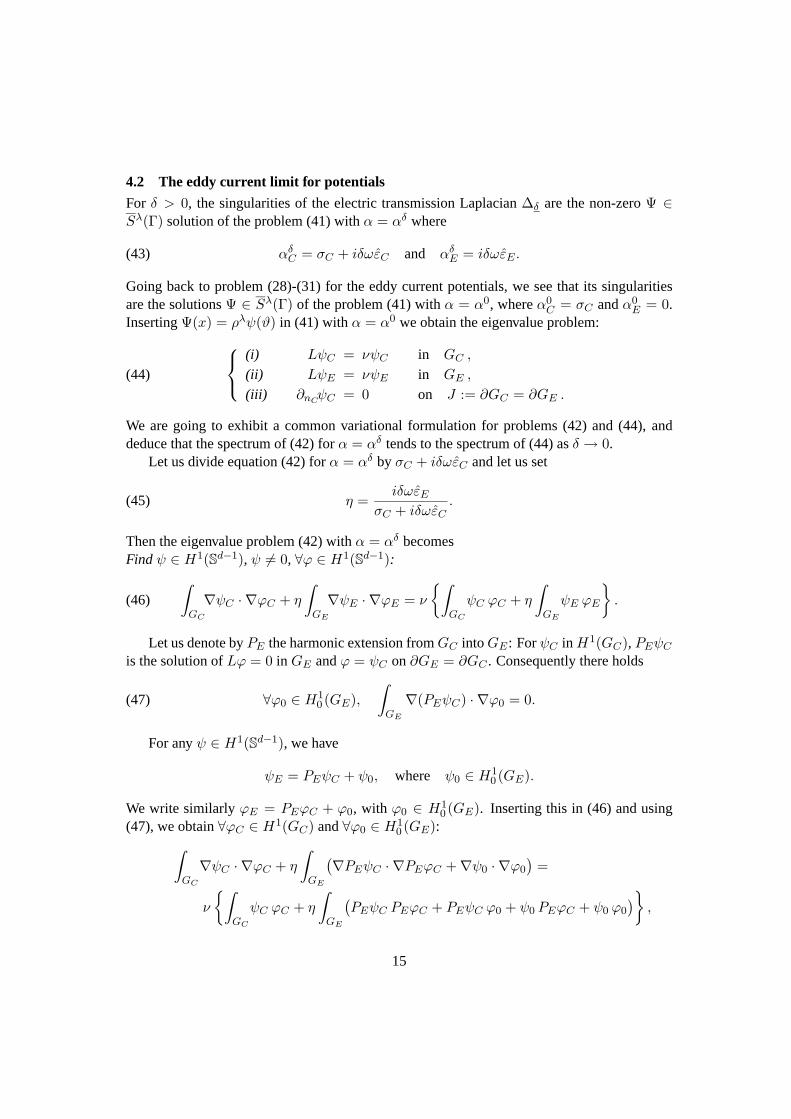
4.2 The eddy current limit for potentials

For δ > 0, the singularities of the electric transmission Laplacian ∆δ are the non-zero Ψ ∈Sλ(Γ) solution of the problem (41) with α = αδ where

αδC = σC + iδωεC and αδ

E = iδωεE .(43)

Going back to problem (28)-(31) for the eddy current potentials, we see that its singularitiesare the solutions Ψ ∈ Sλ(Γ) of the problem (41) with α = α0, where α0

C = σC and α0E = 0.

Inserting Ψ(x) = ρλψ(ϑ) in (41) with α = α0 we obtain the eigenvalue problem:

(i) LψC = νψC in GC ,

(ii) LψE = νψE in GE ,

(iii) ∂nCψC = 0 on J := ∂GC = ∂GE .

(44)

We are going to exhibit a common variational formulation for problems (42) and (44), anddeduce that the spectrum of (42) for α = αδ tends to the spectrum of (44) as δ → 0.

Let us divide equation (42) for α = αδ by σC + iδωεC and let us set

η =iδωεE

σC + iδωεC.(45)

Then the eigenvalue problem (42) with α = αδ becomesFind ψ ∈ H1(Sd−1), ψ = 0, ∀ϕ ∈ H1(Sd−1):∫

GC

∇ψC · ∇ϕC + η

∫GE

∇ψE · ∇ϕE = ν

∫GC

ψC ϕC + η

∫GE

ψE ϕE

.(46)

Let us denote by PE the harmonic extension from GC into GE : For ψC in H1(GC), PEψC

is the solution of Lϕ = 0 in GE and ϕ = ψC on ∂GE = ∂GC . Consequently there holds

∀ϕ0 ∈ H10 (GE),

∫GE

∇(PEψC) · ∇ϕ0 = 0.(47)

For any ψ ∈ H1(Sd−1), we have

ψE = PEψC + ψ0, where ψ0 ∈ H10 (GE).

We write similarly ϕE = PEϕC + ϕ0, with ϕ0 ∈ H10 (GE). Inserting this in (46) and using

(47), we obtain ∀ϕC ∈ H1(GC) and ∀ϕ0 ∈ H10 (GE):∫

GC

∇ψC · ∇ϕC + η

∫GE

(∇PEψC · ∇PEϕC +∇ψ0 · ∇ϕ0

)=

ν

∫GC

ψC ϕC + η

∫GE

(PEψC PEϕC + PEψC ϕ0 + ψ0 PEϕC + ψ0 ϕ0

),

15

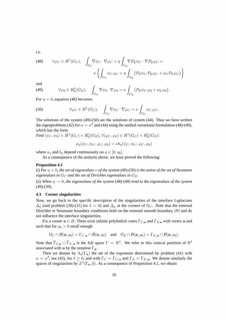
i.e.

∀ϕC ∈ H1(GC),∫GC

∇ψC · ∇ϕC + η

∫GE

∇PEψC · ∇PEϕC =(48)

ν

∫GC

ψC ϕC + η

∫GE

(PEψC PEϕC + ψ0 PEϕC

)

and

∀ϕ0 ∈ H10 (GE),

∫GE

∇ψ0 · ∇ϕ0 = ν

∫GE

(PEψC ϕ0 + ψ0 ϕ0

).(49)

For η = 0, equation (48) becomes

∀ϕC ∈ H1(GC),∫GC

∇ψC · ∇ϕC = ν

∫GC

ψC ϕC .(50)

The solutions of the system (49)-(50) are the solutions of system (44). Thus we have writtenthe eigenproblems (42) for α = αδ and (44) using the unified variational formulation (48)-(49),which has the formFind (ψC , ψ0) ∈ H1(GC)×H1

0 (GE), ∀(ϕC , ϕ0) ∈ H1(GC)×H10 (GE):

aη(ψC , ψ0 ; ϕC , ϕ0) = νbη(ψC , ψ0 ; ϕC , ϕ0)

where aη and bη depend continuously on η ∈ [0, η0].As a consequence of the analysis above, we have proved the following:

Proposition 4.1(i) For η = 0, the set of eigenvalues ν of the system (49)-(50) is the union of the set of Neumanneigenvalues in GC and the set of Dirichlet eigenvalues in GE .

(ii) When η → 0, the eigenvalues of the system (48)-(49) tend to the eigenvalues of the system(49)-(50).

4.3 Corner singularities

Now, we go back to the specific description of the singularities of the interface Laplacians∆δ (and problem (28)-(31) for δ = 0) and ∆µ at the corners of ΩC . Note that the externalDirichlet or Neumann boundary conditions hold on the external smooth boundary ∂Ω and donot influence the interface singularities.

Fix a corner a ∈ B. There exist infinite polyhedral cones ΓC,a and ΓE,a with vertex a andsuch that for ρ0 > 0 small enough

ΩC ∩ B(a, ρ0) = ΓC,a ∩ B(a, ρ0) and ΩE ∩ B(a, ρ0) = ΓE,a ∩ B(a, ρ0).

Note that ΓC,a ∪ ΓE,a is the full space Γ = R3. We refer to this conical partition of R

3

associated with a by the notation Γa.Then we denote by Λδ(Γa) the set of the exponents determined by problem (41) with

α = αδ, see (43), for δ ≥ 0, and with ΓC = ΓC,a and ΓE = ΓE,a. We denote similarly thespaces of singularities by Zλ(Γa, δ). As a consequence of Proposition 4.1, we obtain

16

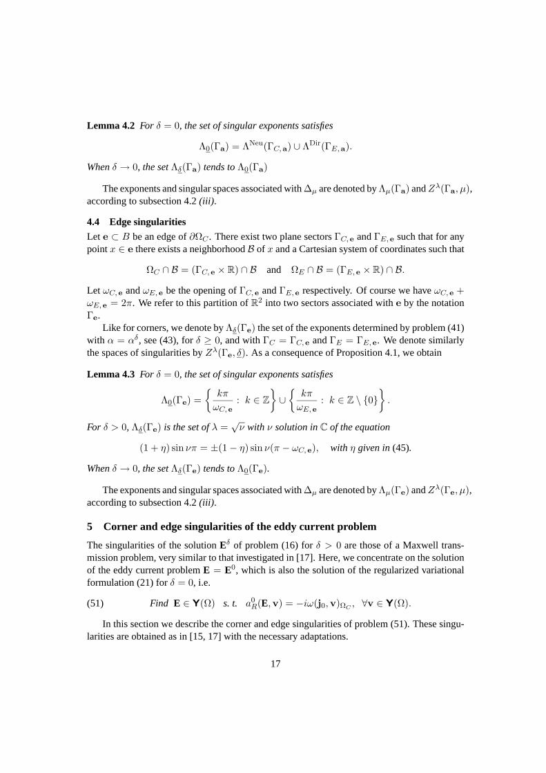
Lemma 4.2 For δ = 0, the set of singular exponents satisfies

Λ0(Γa) = ΛNeu(ΓC,a) ∪ ΛDir(ΓE,a).

When δ → 0, the set Λδ(Γa) tends to Λ0(Γa)

The exponents and singular spaces associated with ∆µ are denoted by Λµ(Γa) andZλ(Γa, µ),according to subsection 4.2 (iii).

4.4 Edge singularities

Let e ⊂ B be an edge of ∂ΩC . There exist two plane sectors ΓC, e and ΓE, e such that for anypoint x ∈ e there exists a neighborhood B of x and a Cartesian system of coordinates such that

ΩC ∩ B = (ΓC, e × R) ∩ B and ΩE ∩ B = (ΓE, e × R) ∩ B.

Let ωC, e and ωE, e be the opening of ΓC, e and ΓE, e respectively. Of course we have ωC, e +ωE, e = 2π. We refer to this partition of R

2 into two sectors associated with e by the notationΓe.

Like for corners, we denote by Λδ(Γe) the set of the exponents determined by problem (41)with α = αδ, see (43), for δ ≥ 0, and with ΓC = ΓC, e and ΓE = ΓE, e. We denote similarlythe spaces of singularities by Zλ(Γe, δ). As a consequence of Proposition 4.1, we obtain

Lemma 4.3 For δ = 0, the set of singular exponents satisfies

Λ0(Γe) =

kπ

ωC, e: k ∈ Z

∪

kπ

ωE, e: k ∈ Z \ 0

.

For δ > 0, Λδ(Γe) is the set of λ =√ν with ν solution in C of the equation

(1 + η) sin νπ = ±(1− η) sin ν(π − ωC, e), with η given in (45).

When δ → 0, the set Λδ(Γe) tends to Λ0(Γe).

The exponents and singular spaces associated with ∆µ are denoted by Λµ(Γe) andZλ(Γe, µ),according to subsection 4.2 (iii).

5 Corner and edge singularities of the eddy current problem

The singularities of the solution Eδ of problem (16) for δ > 0 are those of a Maxwell trans-mission problem, very similar to that investigated in [17]. Here, we concentrate on the solutionof the eddy current problem E = E0, which is also the solution of the regularized variationalformulation (21) for δ = 0, i.e.

Find E ∈ Y(Ω) s. t. a0R(E,v) = −iω(j0,v)ΩC

, ∀v ∈ Y(Ω).(51)

In this section we describe the corner and edge singularities of problem (51). These singu-larities are obtained as in [15, 17] with the necessary adaptations.

17

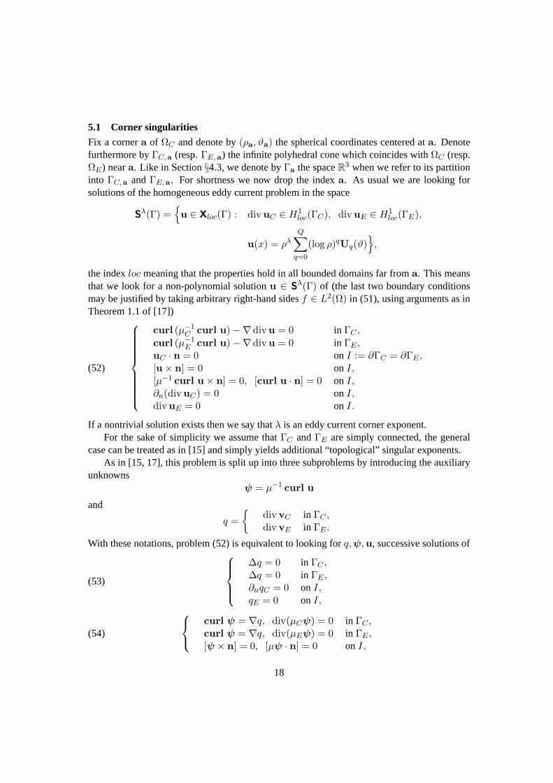
5.1 Corner singularities

Fix a corner a of ΩC and denote by (ρa, ϑa) the spherical coordinates centered at a. Denotefurthermore by ΓC,a (resp. ΓE,a) the infinite polyhedral cone which coincides with ΩC (resp.ΩE) near a. Like in Section §4.3, we denote by Γa the space R

3 when we refer to its partitioninto ΓC,a and ΓE,a. For shortness we now drop the index a. As usual we are looking forsolutions of the homogeneous eddy current problem in the space

Sλ(Γ) =u ∈ Xloc(Γ) : div uC ∈ H1

loc(ΓC), div uE ∈ H1loc(ΓE),

u(x) = ρλQ∑

q=0

(log ρ)qUq(ϑ),

the index loc meaning that the properties hold in all bounded domains far from a. This meansthat we look for a non-polynomial solution u ∈ Sλ(Γ) of (the last two boundary conditionsmay be justified by taking arbitrary right-hand sides f ∈ L2(Ω) in (51), using arguments as inTheorem 1.1 of [17])

curl (µ−1C curl u)−∇div u = 0 in ΓC ,

curl (µ−1E curl u)−∇div u = 0 in ΓE ,

uC · n = 0 on I := ∂ΓC = ∂ΓE ,[u× n] = 0 on I,[µ−1 curl u× n] = 0, [curl u · n] = 0 on I,∂n(div uC) = 0 on I,div uE = 0 on I.

(52)

If a nontrivial solution exists then we say that λ is an eddy current corner exponent.For the sake of simplicity we assume that ΓC and ΓE are simply connected, the general

case can be treated as in [15] and simply yields additional “ topological” singular exponents.As in [15, 17], this problem is split up into three subproblems by introducing the auxiliary

unknownsψ = µ−1 curl u

and

q =

div vC in ΓC ,div vE in ΓE .

With these notations, problem (52) is equivalent to looking for q,ψ,u, successive solutions of

∆q = 0 in ΓC ,∆q = 0 in ΓE ,∂nqC = 0 on I,qE = 0 on I,

(53)

curl ψ = ∇q, div(µCψ) = 0 in ΓC ,curl ψ = ∇q, div(µEψ) = 0 in ΓE ,[ψ × n] = 0, [µψ · n] = 0 on I,

(54)

18

curl u = µCψ, div u = q in ΓC ,curl u = µEψ, div u = q in ΓE ,uC · n = 0 on I,[u× n] = 0 on I.

(55)

This means that we have three types of singularities:Type 1: q = 0, ψ = 0 and u is a general solution of (55).Type 2: q = 0, ψ is a general solution of (54) and u a particular solution of (55).Type 3: q is a general solution of (53),ψ a particular solution of (54) and u a particular solutionof (55).

These three types of singularities may be described with the help of the corner singularitiesof the Neumann problem in ΓC , of the Dirichlet problem in ΓE and of the transmission operator∆µ.

Since for our problem (51), div EC and div EE are regular, we do not describe the singu-larities of type 3 since they cannot occur for any solution of (51).

Let us start with the singularity of type 1:

Lemma 5.1 Assume that λ = −1. Then u ∈ Sλ(Γ) is a singularity of type 1 if and only if (i)or (ii) below holds.(i) λ+1 belongs to ΛNeu(ΓC), u = ∇Φ, with ΦC ∈ Zλ+1

Neu (ΓC) and ΦE ∈ Sλ+1(ΓE) solutionof

∆ΦE = 0 in ΓE ,ΦE = ΦC on I.

(56)

(ii) λ + 1 belongs to ΛDir(ΓE), u = ∇Φ, with ΦC = 0 and ΦE ∈ Zλ+1Dir (ΓE).

Proof: As

curl uC = 0 in ΓC ,

curl uE = 0 in ΓE ,

there exists ΦC ∈ Sλ+1(ΓC) and ΦE ∈ Sλ+1(ΓE) such that

uC = ∇ΦC in ΓC ,

uE = ∇ΦE in ΓE .

From (55) we deduce that

∆ΦC = 0 in ΓC ,∆ΦE = 0 in ΓE ,∂nΦC = 0 on I,ΦC = ΦE on I.

Then either ΦC is not zero and we are in the case (i) or ΦC = 0 and we are in the case(ii).

19

Lemma 5.2 Assume that λ > 0. Then u ∈ Sλ(Γ) is a singularity of type 2 if and only if λbelongs to Λµ(Γ), ψ = ∇Ψ, with Ψ ∈ Zλ(Γ, µ) and u given by

u =1

λ + 1(µ(∇Ψ× x) +∇r) ,(57)

where rC ∈ Sλ+1(ΓC), rE ∈ Sλ+1(ΓE) are solutions of

∆rC = 0 in ΓC ,∆rE = 0 in ΓE ,∂nrC = −µC(∇ΨC × x) · n on I,rC = rE on I.

(58)

Proof: As

curl ψC = 0 in ΓC ,

curl ψE = 0 in ΓE ,

there exists ΨC ∈ Sλ(ΓC) and ΨE ∈ Sλ(ΓE) such that

ψC = ∇ΨC in ΓC ,

ψE = ∇ΨE in ΓE .

From (54) we deduce that

div(µC∇ΨC) = 0 in ΓC ,div(µE∇ΨE) = 0 in ΓE ,[Ψ] = 0, [µ∂nΨ] = 0 on I.

This means that Ψ ∈ Zλ(Γ, µ).Now we readily check that u in the form (57) is solution of (55) if and only if r is solution

of (58), whose solution exists by Theorem 4.14 of [27].

Lemma 5.3 (i) λ = −1 is not a corner singularity of type 1.(ii) λ = 0 is not a corner singularity of type 2.

Proof:(i) If u is a singularity of type 1 for λ = −1, then uC is a singularity of type 1 for λ = −1 forthe Maxwell system in ΓC with the boundary condition uC ·n = 0 on I . Therefore by Lemma7.8 of [15] uC = 0. With this information, uE is now a singularity of type 1 for λ = −1 forthe Maxwell system in ΓE with the boundary condition uE × n = 0 on I . Again by Lemma7.8 of [15] we get uE = 0.

(ii) If u is a singularity of type 2 for λ = 0, then ψ = µ−1 curl uC is a singularity of type 1for λ = −1 for the Maxwell interface system in R

3 with the parameter µ. Therefore by Lemma5.4 of [17] we get ψ = 0.

20

Since the singularities of our problem (51) have to be locally in X(Γ) with a piecewisesmooth divergence, among the singular exponents described above, we select the subset Λa ofλ > −3

2 such that there exists u ∈ Sλ(Γ) solution of (52) such that

χu ∈ X(Γ),

where χ is a cut-off function equal to 1 near a. This last condition implies the followingconstraints for our two types of singularities (see [17]):

Type 1: λ+1 ∈ ΛNeu(ΓC) or λ+1 ∈ ΛDir(ΓE) and since ΛDir(ΓE)∩[−1, 0] and ΛNeu(ΓC)∩[−1, 0] are empty, by Lemma 5.3 we get λ > −1.

Type 2: λ ∈ Λµ(Γ) and by the condition curl (χu) ∈ [L2(R3)]3, we get λ > −12 . By Lemma

5.3 and the fact that Λµ(Γ) ∩ [−1, 0] is empty, we get λ > 0.In conclusion we have

Λa = λ > −1 : λ + 1 ∈ ΛNeu(ΓC) ∪ λ > −1 : λ + 1 ∈ ΛDir(ΓE)∪ λ > 0 : λ ∈ Λµ(Γ).

5.2 Edge singularities

Fix an edge e of ΩC and denote by ΓC ×R (resp. ΓE ×R) the infinite polyhedral cone whichcoincides with ΩC (resp. ΩE) near e (ΓC and ΓE are then two-dimensional sectors). Denoteby (r, θ, z) the cylindrical coordinates along e. As before we are looking for solutions of thehomogeneous eddy current problem (52) in ΓC × R and ΓE × R. Now Γ refers to R

2 withits partition into the two sectors ΓC and ΓE , cf Section 4.4. Writing u = (v, w), where v arethe first two components of u in the Cartesian coordinates (x1, x2, x3) (according to the abovenotation, the x3-axis contains the edge e), the system (52) is split up into the following twoindependent problems in R

2:

curl (µ−1C curlv)−∇div v = 0 in ΓC ,

curl (µ−1E curlv)−∇div v = 0 in ΓE ,

vC · n = 0 on I := ∂ΓC = ∂ΓE ,[v × n] = 0 on I,[µ−1 curlv × n] = 0 on I,∂n(div vC) = 0 on I,div vE = 0 on I.

(59)

div(µ−1C ∇wC) = 0 in ΓC ,

div(µ−1E ∇wE) = 0 in ΓE ,

[w] = 0, [µ−1∂nw] = 0 on I.

(60)

Problem (60) is a standard transmission problem whose set of singularities Λµ−1(Γ) =Λµ(Γ) (see Lemma 6.2 of [17]) were described in section 4. Problem (59) is a two-dimensional

21

eddy current problem whose singularities may be described as in 3D, by introducing the auxil-iary unknowns ψ = µ−1 curlv and

q =

div v in ΓC ,div v in ΓE .

As before, singularities of type 1, 2 and 3 then appear. We can show that singularities of type 2do not exist (compare with [15, 17]), singularities of type 3 are not studied for the same reasonas before, while singularities of type 1 are analyzed exactly as in Lemma 5.1.

In conclusion we can state the following result.

Lemma 5.4 The set Λe of edge exponents associated with e is given by

Λe = λ > −1 : λ + 1 ∈ ΛNeu(ΓC) ∪ λ > −1 : λ + 1 ∈ ΛDir(ΓE)∪ λ > 0 : λ ∈ Λµ(Γ).

If λ ∈ N \ 0, then the associated singular function u = (v, w) is as follows:

• If λ + 1 ∈ ΛNeu(ΓC), then w = 0,

vC = ∇(rλ+1ϕC

),

with ϕC(θ) = cos((λ + 1)θ) (the half-lines θ = 0 and θ = ωC are assumed to be theinterfaces between ΓC and ΓE , the interior opening of ΓC (resp. ΓE) is then ωC (resp.ωE = 2π − ωC)), and if ωE

ωCis not a rational number, then

vE = ∇(rλ+1ϕE

),

with ϕE(θ) = c1 cos((λ + 1)θ) + c2 sin((λ + 1)θ), for some (explicit) constants c1 andc2. If ωE

ωCis a rational number, then a logarithmic term possibly appears in the expression

of vE .

• If λ + 1 ∈ ΛDir(ΓE), then w = 0, vC = 0 and

vE = ∇(rλ+1ϕE

),

with ϕE(θ) = sin((λ + 1)(θ − ωC)).

• If λ ∈ Λµ(Γ), then v = 0 and w = rλϕ, with ϕ an eigenvector of problem (42) forα = µ, associated with the eigenvalue ν = λ2.

6 Regularity and singularity results for the eddy current problem

We describe the regularity as well as singular decompositions of any solution E of the regular-ized problem (51) with a source current density j0 such that

div j0 = 0, supp j0 ⊂ ΩC , j0 ∈ [Hs−1(ΩC)]3 for s ≥ 1.(61)

These results are based on the knowledge of corner and edge singularities described in theprevious section and rely on the application of Mellin techniques as in [15, 17].

22

6.1 Regularity

For any corner a in the interface B introduce

λNeuC,a = minλ > 0 : λ ∈ ΛNeu(ΓC,a),

λDirE,a = minλ > 0 : λ ∈ ΛDir(ΓE,a),λµ,a = minλ > 0 : λ ∈ Λµ(Γa),

where Λµ(Γa) is defined in section 4.3 for the subdivision of R3 into ΓC,a and ΓE,a. Similarly

for any edge e ⊂ B define

λµ,e = minλ > 0 : λ ∈ Λµ(Γe).

Now we can set

τ(1)e := min

(π

ωC, e,

π

ωE, e

),

τ(1)a := min

(λNeuC,a , λDir

E,a

),

τ (1) := min(

mine

τ(1)e ,

12

+ mina

τ(1)a

),

τ(1)C := min

(min

e

π

ωC, e,

12

+ mina

λNeuC,a

),

τ (2) := min(

mine

λµ,e ,12

+ mina

λµ,a

),

when ωC, e is the opening of ΩC along e and ωE, e = 2π− ωC, e is the opening of ΩE along e.Then we have

Theorem 6.1 Let E ∈ Y(Ω) be a solution of problem (51) with j0 satisfying (61) for s ≥ 1.Then we have

EC ∈ HτC (ΩC), ∀τC < min

(τ

(1)C , τ (2) + 1, s + 1

),

EE ∈ HτE (ΩE), ∀τE < min

(τ (1), τ (2) + 1, s + 1

).

6.2 Singularities

We start with a general result and then restrict ourselves to a particular case where there remainonly singularities of type 1.

The general result is proved exactly as in [15, 17] and can be stated as follows:

Theorem 6.2 Assume that s ≥ 1 such that for all corners a, s− 12 does not belong to Λa and

for all edges e, s does not belong to Λe. Assume furthermore that the edge exponents in [−1, s]are contained in an interval of length < 1. Let E ∈ Y(Ω) be a solution of problem (51) with j0satisfying (61) for this regularity exponent s. Then E admits the decomposition

E = E(R) + E(S),(62)

23

where the regular part satisfies

E(R)C ∈ Hs+1(ΩC) and E(R)

E ∈ Hs+1(ΩE).

On the other hand the singular part E(S) has the standard structure

E(S) =∑a

∑λ∈Λa∩ [− 3

2,s− 1

2]

∑p

γλ,pa χa(ρa)uλ,p

a (ρa, ϑa)(63)

+∑e

∑λ∈Λe∩ [−1,s]

∑p

K[γλ,pe ]χe(ρe)uλ,p

e (ρe, θe),(64)

where uλ,pa (resp. uλ,p

e ) are the corner (resp. edge) singularities of type 1 or 2 described in theprevious section, χa (resp. χe) is a smooth cut-off function equal to 1 near ρ = 0, ρe = red

−1e

when de is a smooth function which is equivalent to the distance of the endpoints of e, K is aconvolution operator (cf. [18, 15, 17]) and γλ,p

a (resp. γλ,pe ) are real constant (resp. functions

defined in the edge e and belonging to some weighted Sobolev spaces).

Exactly as in [15, 17], if one wants to eliminate the singularities of type 2, we introduce aparameter τ ≤ s satisfying

τ < minτ (1), τ (2).(65)

Using Lemmas 4.11 and 4.13 of [15], we obtain

Theorem 6.3 Let E ∈ Y(Ω) be a solution of problem (51) with j0 as in the introductionand the regularity j0 ∈ [Hs−1(ΩC)]3 with s ≥ 1. Let τ ≤ s satisfy (65) and such thatthe edge exponents in [−1, τ ] are contained in an interval of length < 1. Then E admits thedecomposition

E = E(R) +∇Φ,

where the regular part satisfies

E(R)C ∈ Hτ+1(ΩC) and E(R)

E ∈ Hτ+1(ΩE),

while Φ ∈ H1(Ω) satisfies

∆ΦC ∈ Hτ (ΩC)∂nΦC = 0 on B,

and

∆ΦE ∈ Hτ (ΩE),ΦE = ΦC on B.

If τ = 0 the above theorem reduces to Theorem 3.1. For τ not necessarily equal to zero,as in that Theorem, ΦC has the singularities of the interior Neumann problem, while ΦE hasinduced exterior singularities as well as exterior Dirichlet ones.

24

7 Continuity of the singular functions in the eddy current limit

If we put together

1. The result of Section 4.2 which yields the continuity of the singular exponents withrespect to δ for the associated scalar problem,

2. The common structure of Maxwell and eddy current singularities of Type 1 (as gradientsof scalar singularities),

3. The similar structure of Maxwell and eddy current singularities of Type 2 (compare ourLemma 5.2 with [17, Lemma 5.2]),

we may wonder whether it is possible to define a basis of singular fields uλ,pa [δ] and uλ,p

e [δ] forthe eddy current problem (51), δ = 0, and the Maxwell problem (21), δ > 0, which should beregular with respect to δ ∈ [0, δ0] and so that a decomposition like that of Theorem 6.2 holdswith coefficients depending smoothly on δ.

In this paper, we will not address this question in its full complexity, but show that it ispossible to choose bases of singular functions in a regular way with respect to δ, up to thelimit δ = 0. This means that we have mainly to investigate the behavior of all singularities(i.e. in Sλ(Γ)) of the scalar problems (40) when α = αδ given by (43), as δ → 0. Similarquestions are addressed in [13, 14, 28]. Since the direct application of these references is notstraightforward, we are going to state the main steps of a relevant construction.

In the general case, we cannot exclude any of the phenomena such as “crossing” and“branching” that appear for singularity problems depending on a parameter. Since, in our sit-uation, the coefficients are non-real, we may expect singularity exponents that have algebraicbranch points for certain values of δ, even for δ = 0, i.e. in the eddy current limit. We alsocan have changes of multiplicities, even for δ = 0, for example in the case where a singularexponent for the Neumann problem in ΓC coincides with a singular exponent for the Dirichletproblem in ΓE .

In both these situations, any individual singular function of the transmission problem ∆δ

of the form ρλδψδ(ϑ) will converge to a singular function ρλ0ψ0(ϑ) of the limit problem, butthe coefficients of a such singular function may be non-regular with respect to δ or even blowup for δ → 0. Clustering several singular functions together and choosing a basis dependinganalytically on δ as explained below in Section 7.2 will avoid such pathologies.

7.1 Mellin symbols

It is known from [23] that the corner singularities solution of (41) are produced by the poles ofthe associated Mellin symbol: Let us recall that the Mellin symbol of an operator A homoge-neous of degree m with constant coefficients is λ → A(λ) where

A(∂x) = ρ−mA(ϑ; ρ∂ρ, ∂ϑ) and A(λ) := A(ϑ;λ, ∂ϑ).

25

Let us consider the situation of threedimensional cones (d = 3). The symbol associated withthe operator (40) – see also (41), is

ψ −→

LψC − λ(λ + 1)ψC in GC ,

LψE − λ(λ + 1)ψE in GE ,

αC∂nCψC + αE∂nEψE on J := ∂GC = ∂GE .

(66)

Let us denote by Mα(λ) the operator (66) acting between function spaces:

Mα(λ) : Z(GC , GE) −→ L2(GC)× L2(GE)×H−1/2(J) ,

where the source space Z(GC , GE) is defined as

Z(GC , GE) =ϕ ∈ H1(S2) : ∆ϕC ∈ L2(GC), ∆ϕE ∈ L2(GE)

.

When α = αδ is given by (43), we denote Mα(λ) by Mδ(λ).We are going to prove that for all δ ∈ [0, δ0] there exists λ such that Mδ(λ) is invertible. Let

(fC , fE , g) belong to L2(GC)×L2(GE)×H−1/2(J) and let us fix λ such that−λ(λ+1) > 0.

• If δ = 0, we first solve the Neumann problem(L− λ(λ + 1)

)ψC = fC in GC ,

αC∂nCψC = g on J

and then the Dirichlet problem(L− λ(λ + 1)

)ψE = fE in GE ,

ψE = ψC

∣∣J

on J

• If δ > 0, we use a variational formulation as in (42): ∀ϕ ∈ H1(Sd−1),∫Sd−1

α∇ψ · ∇ϕ− λ(λ + 1)∫

Sd−1

αψϕ =∫GC

fCϕC +∫GE

fEϕE +∫Jgψ.

Since the right hand side is clearly in H−1(Sd−1), the coerciveness yields a unique solu-tion.

The analytic Fredholm theorem yields that for all δ ∈ [0, δ0], λ → Mδ(λ)−1 is meromor-phic. As the dependency of the symbol on δ is analytic, such is also the case for its inverse.

7.2 Stable bases for singularities

Let δ ∈ [0, δ0] be fixed. We recall that we have denoted by Λδ(Γ) the set of the singularexponents of the operator ∆δ (transmission or coupling).

The singular exponents in Λδ(Γ) coincide with the poles λ0 of Mδ(λ)−1. Moreover thecorresponding space of singularities Zλ0(Γ; δ) (the space of solutions in Sλ0(Γ) of (41) forα = αδ) is also given by a Cauchy residue formula:

Zλ0(Γ; δ) =

Ψ : ∃F ∈ O(D(λ0)), Ψ =1

2iπ

∫∂D(λ0)

ρλMδ(λ)−1F (λ) dλ

where

26

• D(λ0) is a disc in the complex plane centered in λ0 and not containing any other pole ofMδ(λ)−1;

• The notation F ∈ O(D(λ0)) means that λ → F (λ) is holomorphic in a neighborhoodof D(λ0) with values in the target space L2(GC)× L2(GE)×H−1/2(J).

Note that if D contains several elements of Λδ(Γ), but ∂D ∩ Λδ(Γ) is empty, then

Ψ : ∃F ∈ O(D), Ψ =

12iπ

∫∂D

ρλMδ(λ)−1F (λ) dλ

=⊕

λ∈Λδ(Γ)∩D

Zλ(Γ; δ).

The smooth dependency on δ of Mδ(λ)−1 implies the principle of smooth dependency ofthe singular spaces Zλ(Γ; δ) on δ in the following sense: Since we are interested in the eddycurrent limit let us consider a pole λ0 of M0(λ)−1 and a disc D = D(λ0) such that λ0 is theonly pole of M0(λ)−1 in D. There exists δ(λ0) such that for all δ ∈ [0, δ(λ0)] the symbolsMδ(λ)−1 are invertible on ∂D. Then the spaces

Ψ : ∃F ∈ O(D), Ψ =

12iπ

∫∂D

ρλMδ(λ)−1F (λ) dλ,(67)

depend smoothly on δ up to the limit δ = 0. In other words⊕λ∈Λδ(Γ)∩D

Zλ(Γ; δ) −→δ→0

Zλ0(Γ; 0).

Indeed, this statement shows the necessity of keeping together some clusters of poles.We obtain easily a basis depending smoothly on δ: Choose F 1, . . . , Fm inO(D) such that

Ψn0 (ρ, ϑ) :=

12iπ

∫∂D

ρλM0(λ)−1Fn(λ) dλ, n = 1, . . . ,m

is a basis of Zλ0(Γ; 0). Then, for δ small enough the functions

Ψnδ (ρ, ϑ) :=

12iπ

∫∂D

ρλMδ(λ)−1Fn(λ) dλ, n = 1, . . . ,m

are a basis of⊕

λ∈Λδ(Γ)∩D Zλ(Γ; δ). The mappings δ → Ψnδ are analytic with respect to

δ ∈ [0, δ0].

7.3 Simple singularities

If the dimension of Zλ0(Γ; 0) is 1, or more generally if δ = 0 is not a point of crossingor branching for the singularities, then the behavior of individual singular functions is verysimple indeed. Let us consider the two typical situations where this happens:

27

1. If λ0 ∈ ΛDir(ΓE) is a simple eigenvalue and such that λ0 ∈ ΛNeu(ΓC), then we can finda unique λδ ∈ Λδ(Γ) such that δ → λδ is analytic for δ in a neighborhood of 0. If wefix a ρλ0ψ0 in the singular space Zλ0

Dir(ΓE), then we find a generator ρλδψδ of Zλ(Γ; δ)such that δ → ψδ is analytic for δ small enough. Then ψδ,C → 0 on GC in H1(GC) andψδ,E → ψ0,E on GE in H1(GE).

2. If λ0 ∈ ΛNeu(ΓC) \ ΛDir(ΓE), we have a singular function ρλδψδ with δ → λδ andδ → ψδ analytic. Here ρλ0ψ0,C is a singular function of the Neumann problem in ΓC

and ψ0,E is the harmonic extension of ψ0,C to S2.

Situation 1., resp. 2., occurs for the first corner singularity of the eddy current problemwhere ΩC has a corner like a cube, resp. like the exterior of a cube.

Situation 1. or 2. always occurs for the first edge singularity where the exponent is

λ = min

π

ωC,π

ωE

− 1,

because π/ωC and π/ωE = π/(2π − ωC) never coincide. Although unpredictable in general,the simplicity of limiting exponents of singularity is generic.

References

[1] A. Alonso and A. Valli, A domain decomposition approach for heterogeneous time-harmonic Maxwell equations, Comput. Meth. Appl. Mech. Engrg, 143, 1997, 97-112.

[2] A. Alonso-Rodriguez, F. Fernandes and A. Valli, Weak and strong formulations for thetime-harmonic eddy-current problem in general domains, Report UTM, 603, Diparti-mento di Matematica, Univ. di Trento, Italy, 2001.

[3] H. Ammari, A. Buffa and J.-C. Nedelec, A justification of eddy currents model for theMaxwell equations, SIAM J. Appl. Math., 60, 2000, 1805-1823.

[4] C. Amrouche, C. Bernardi, M. Dauge and V. Girault, Vector potentials in three-dimensional nonsmooth domains, Math. Meth. Applied Sc., 21, 1998, 823-864.

[5] F. Assous, P. Ciarlet Jr. and E. Sonnendrucker, Resolution of the Maxwell equations in adomain with reentrant corners, RAIRO Model. Math. Anal. Numer., 32, 1998, 359-389.

[6] R. Beck, R. Hiptmair, R.H.W. Hoppe and B. Wohlmuth, Residual based a posteriori errorestimators for eddy current computation, RAIRO Model. Math. Anal. Numer., 34, 2000,159-182.

[7] M. Birman and M. Solomyak, L2-theory of the Maxwell operator in arbitrary domains,Russian Math. Surv., 42, 1987, 75-96.

[8] M. Birman and M. Solomyak, On the main singularities of the electric component of theelectro-magnetic field in regions with screens, St. Petersbg. Math. J., 5, 1993, 125-139.

28

[9] A.-S. Bonnet-Ben Dhia, C. Hazard and S. Lohrengel, A singular field method for thesolution of Maxwell’s equations in polyhedral domains, SIAM J. Appl. Math., 59, 1999,2028-2044.

[10] A. Bossavit, Two dual formulations of the 3D eddy-current problem, COMPEL, 4, 1985,103-116.

[11] A. Bossavit, Electromagnetisme en vue de la modelisation, Springer Verlag, 1993.

[12] D. Colton and R. Kress, Integral equation methods in scattering theory. Pure and AppliedMathematics. John Wiley & Sons, Inc., New York, 1983

[13] M. Costabel and M. Dauge, Singularites d’aretes pour les problemes aux limites ellip-tiques. In Journees “Equations aux Derivees Partielles” (Saint-Jean-de-Monts, 1992).Ecole Polytech., Palaiseau, 1992, Exp. No. IV, 12p.

[14] M. Costabel and M. Dauge, Stable asymptotics for elliptic systems on plane domains withcorners. Comm. Partial Differential Equations no 9 & 10, 1994, 1677-1726.

[15] M. Costabel and M. Dauge, Singularities of Maxwell’s equations on polyhedral domains,Arch. Rational Mech. Anal., 151, 2000, 221-276.

[16] M. Costabel and M. Dauge, Weighted regularization of Maxwell equations in polyhedraldomains A rehabilitation of nodal finite elements, Numer. Math., 93, 2002, 239-277.

[17] M. Costabel, M. Dauge and S. Nicaise, Singularities of Maxwell interface problems,RAIRO Model. Math. Anal. Numer., 33, 1999, 627-649.

[18] M. Dauge, Elliptic boundary value problems on corner domains, L.N. in Math., 1341,Springer-Verlag, Berlin, 1988.

[19] M. Dobrowolski, Numerical approximation of elliptic interface and corner problems, Ha-bilitationsscrift, Bonn, Germany, 1981.

[20] V. Girault and P.-A. Raviart, Finite element methods for Navier-Stokes equations,Springer Series in Comp. Math. 5, Springer-Verlag, 1986.

[21] P. Grisvard, Elliptic problems in nonsmooth domains, Monographs and Studies in Math-ematics, 24, Pitman, Boston, 1985.

[22] R. Hiptmair, Symmetric coupling for eddy currents problems, SIAM J. Numer. Anal., 40,2002, 41-65.

[23] V. A. Kondrat’ev, Boundary-value problems for elliptic equations in domains with conicalor angular points, Trans. Moscow Math. Soc., 16, 1967, 227-313.

[24] D. Leguillon and E. Sanchez-Palencia, Computation of singular solutions in elliptic prob-lems and elasticity, RMA, 5, Masson, Paris, 1991.

29

[25] D. Mercier, Minimal regularity of the solutions of some transmission problems, Math.Meth. Appl. Sci., 26, 2003, 321-348.

[26] J.-C. Nedelec, Acoustic and electromagnetic equations, Applied Math. Sc., 144, Springer-Verlag, 2001.

[27] S. Nicaise, Polygonal interface problems, Peter Lang, Berlin, 1993.

[28] S. Nicaise and A.-M. Sandig, General interface problems I,II, Math. Meth. Appl. Sci.,17, 1994, 395-450.

[29] S. Nicaise and A.-M. Sandig, Transmission problems for the Laplace and elasticity opera-tors: Regularity and boundary integral formulation, Mathematical Models and Methodsin Applied Sciences, 9, 1999, 855-898.

[30] S. Nicaise, Edge elements on anisotropic meshes and approximation of the Maxwell equa-tions, SIAM J. Numer. Analysis, 39, 2001, 784-816.

[31] R. Picard, Zur Theorie des harmonischen Differentialformen, Manuscr. Math., 27, 1979,31-45.

[32] R. Picard, On the boundary value problems of electro- and magnetostatics, Proc. RoyalSoc. Edinburgh, 92 A, 1982, 165-174.

Acknowledgement. This work was completed while the first two authors were visiting theNewton Institute for Mathematical Sciences, Cambridge, UK.

Authors adresses.

M. COSTABEL & M. DAUGE : IRMAR, Universite de Rennes 1Campus de Beaulieu, 35042 Rennes Cedex, Francehttp://perso.univ-rennes1.fr/martin.costabel

http://perso.univ-rennes1.fr/monique.dauge

S. NICAISE : Universite de Valenciennes et du Hainaut CambresisMACS, Le Mont Houy, 59313 Valenciennes Cedex 9, Francehttp://www.univ-valenciennes.fr/macs/Serge.Nicaise

30