Singlet axial-vector coupling constant of the nucleon in QCD without instantons!!

! ! ! ! Janardan Prasad Singh! Physics Department, Faculty of Science, ! The M. S. University of Baroda, Vadodara-390002, India!!ABSTRACT!

We have analyzed axial-vector current-current correlation functions between one-nucleon states to calculate the singlet axial-vector coupling constant of the nucleon. The octet-octet and the octet-singlet current correlators, investigated in this work, do not require any use of instanton effects. The QCD and hadronic parameters used for the evaluation of correlators have been varied by (10 - 20)%. The value of the singlet axial-vector coupling constant of the nucleon obtained from this analysis is consistent with its current determination from experiments and QCD theory. !!1. Introduction!

Knowledge of axial-vector coupling constants of the nucleon has a crucial role in !

understanding its longitudinal spin structure [1-4]. In a generalization of Goldberger-Treiman

relation, poorly determined pseudo scalar couplings of the nucleon and are related to

the singlet coupling constant and the eighth component of SU(3) octet coupling constant

[5-7 ]. Among the three flavor-diagonal coupling constants , the isovector coupling

constant is the best understood and is measured from nuclear � -decay. The eighth

component is determined from the analysis of hyperon -decay in SU(3)f symmetry limit .

Indeed, in terms of SU(3)f parameters F and D, these two axial coupling constants are

expressed as !

! ,! !

and determined to be as [8,9]!

, !

β

β

�1

gAa

gA3

(a = 3,8,0)

gA3 = F + D gA

8 = 3F − D

gA3 = 1.270 ± 0.003 gA

8 = 0.58 ± 0.03

gηNN g ′η NN

gA0 gA

8

gA8

However, SU(3)f symmetry may be badly broken and an error in from 10% [10] to 20% [11]

has been suggested. There is no direct way to measure . Theoretically, its calculation is

challenging on account of its association with chiral anomaly. The first moment of spin-

dependent structure function g1 of the nucleon can be related to the scale-invariant axial-vector

coupling constants of the target nucleon. The experimental value of is

obtained from measurement of g1 and combining its first moment integral with the measured

values of and and theoretical calculation of the perturbative QCD Wilson coefficients.

Using SU(3)f symmetric value for and with no leading twist subtraction in the dispersion

relation for polarized photon-nucleon scattering, COMPASS found[12] !

!

Several approaches have been used to calculate axial-vector coupling constants of the

nucleon. Instantons, through axial anomaly relation, is believed to have an important role in the

singlet axial-vector coupling constant of the nucleon [13]. Using numerical simulations of

instanton liquid, Schaffer and Zetocha [14 ] have calculated axial-vector coupling constants of

the nucleon. Though, they get a good result for , for the singlet case they get .

Using lattice QCD, Yang et al. have estimated the part of the proton spin carried by light quarks

from anomalous Ward identities as � =0.30(6) [15]. It hints to suggest that the culprit of the

‘proton spin crisis’ is the U(1)A anomaly. Chiral constituent quark model also gives a good

result for and , but for the singlet case, it gives [16] . In a hybrid approach,

where one takes into account one gluon exchange as well as effect of meson cloud, it has been

possible to get a reasonably good result such as = 0.42 [17]. Similar result for quark spin

contribution to the spin of the nucleon has been obtained using a spin-flavor based

parametrization of QCD [18]. Three different approaches have been followed in QCD sum rule

to calculate axial coupling constant of the nucleon. Ioffe and Oganesian [19] have used the

standard QCD sum rule in external fields. Two-point correlation function of nucleon interpolating

Σ

�2

gA8

gA0

gAa (a = 3,8,0) gA

0

gA3 gA

8

gA8

gA0 = 0.33± 0.03(stat.)± 0.05(syst.)

gA3 gA

0 = 0.77

gA3 gA

8 gA0 ! 0.52

gA0

fields has been evaluated in the presence of a weak axial vector field. The limits on � , the part

of proton spin carried by light quarks, and � , the derivative of the QCD susceptibility have

been found from self-consistency of the sum rule. Belitsky and Teryaev [20] considered a three-

point function of nucleon interpolating fields and the divergence of singlet axial-vector current .

The form factor is related to vacuum condensates of quark-gluon composite operators

through a double dispersion relation. In this approach, the extrapolation to involves large

uncertainties. In the third approach by Nishikawa et al. [21,22], a two-point correlation function

of axial-vector currents in one-nucleon state is evaluated. Here, the axial-vector coupling

constants of the nucleon are expressed in terms of � -N and K-N sigma terms and moments of

parton distributions. The perturbative contribution is subtracted from the beginning and the

continuum contribution can be reduced to a small value. The application of this method using

singlet-singlet axial-vector current correlator for requires taking into account the chiral

anomaly [21]. This gives appreciably high value of . The result was improved by the

inclusion of instantons in the QCD evaluation of correlation function [22]. However, the result

was extremely sensitive to critical instanton size and was not stabilized. Our own experience of

working with singlet-singlet axial-vector current correlator, albeit in vacuum state [23,24 ], is that

the sum rule does not work satisfactorily even on inclusion of instanton contribution. On the

other hand, octet-octet and octet-singlet axial-vector current correlators work well. Instanton

contribution is not needed in these last two sum rules. In view of this, in this work we will

investigate octet-octet and octet-singlet axial-vector current correlators in one-nucleon states.

The results of the two sum rules can be combined to get and . The numerical evaluation

of the sum rules requires use of several QCD and hadronic parameters. We have also studied

consequences of variation of these parameters on sum rules.!

!

!

Σ

′χ (0)

π

�3

gA0 (q2 )

gA0 (0)

gA0

gA0 ≈ 0.8

gA8 gA

0

2. The sum rules!

Following [21,22 ], we consider the correlation functions of axial-vector currents in one-nucleon

states:!

! ! ! ! ! ! ! ! ! ! ! (1)!

where!

! ! ! ! ! ! (2)!

! ! ! ! ! ! ! ! ! ! (3a)!

! ! ! ! ! ! ! ! ! ! ! (3b)! !

!

Actually, has two kinds of contributions: the connected and the disconnected terms.

Unlike the case of singlet-singlet correlator, the disconnected terms do not contribute to octet-

octet as well as to octet-singlet correlators. Hence, the instanton contribution is not needed in

our calculation. Eq.(1) can be written using Lehmann representation as !

! ! ! ! ! ! ! ! ! ! ! ! (4)!

where ! is the spectral function. We take Borel transform of even part in � of both sides

of Eq. (4)!

! ! ! ! (5)!

where � . The nucleon matrix element of axial-vector

current is given as!

(6a)!

!

! ! ! (6b)!

ω

B̂ =−ω 2→∞,n→∞,−ω 2 /n=slim

−ω 2( )n+1n!

− dd(−ω 2 )

⎡⎣⎢

⎤⎦⎥

n

�4

Πµνab (q;P) = i d 4x∫ eiqx T jµ5

a (x), jν 5b (0)⎡⎣ ⎤⎦ N

;

.... N = 12

PS .... PS − .... 0 PS PS⎡⎣ ⎤⎦S∑

jµ58 = 1

6u µγ 5γ u + d µγ 5γ d − 2s µγ 5γ s( )

jµ50 = 1

3u µγ 5γ u + d µγ 5γ d + s µγ 5γ s( )

Πµνab

Πµνab (ω ,q

!;P) = dω '

ρµνab (ω ',q

!;P)

ω −ω '−∞

∞

∫ ,

ρµνab

B̂ Πµνab (ω ,q

!;P)even⎡⎣ ⎤⎦ = − d

−∞

∞

∫ ′ω ′ω e− ′ω 2 /sρµνab ( ′ω ,q

!;P)

P,S Jµ58 ′P , ′S = 1

6u(P,S) gA

8 (q2 )γ µ 5γ + hA8 (q2 )qµ 5γ⎡⎣ ⎤⎦u( ′P , ′S )

P,S Jµ50 ′P , ′S = 1

3u(P,S) gA

0 (q2 )γ µ 5γ + hA0 (q2 )qµ 5γ⎡⎣ ⎤⎦u( ′P , ′S )

(a,b) = (8,0)

Calling ! and realizing that has no singularity at �

one gets! !

� ! ! ! ! ! ! ! ! (7a)!

� ! ! ! ! ! ! ! ! (7b)!

We have calculated correlation functions using operator product expansion (OPE) by

accounting for operators up to dimension 6. Our results for ! has some differences from

those obtained in Ref.[21]. !

! !

!!!!!! ! ! ! ! ! ! ! ! ! ! (8a)!

! !

!

!!!!!! (8b)!

q2 = 0,

∂∂q! 2 B̂ Π88 (ω ,q

!)⎡⎣ ⎤⎦q!2=0 = − 1

21M

gA8 2

∂∂q! 2 B̂ Π80 (ω ,q

!)⎡⎣ ⎤⎦q!2=0 = − 1

21MgA8gA

0

�5

Πab (ω ,q!) =Πµ

abµ (ω ,q!;M ,0!) hA

a (q2 )

Πµνab

Π88 (q2 )

Π88 (q2 )= 1610q2

mu uuN+md dd

N+ 4ms ss N( )⎡

⎣⎢− 321q2

α s

πG2

N

−8 qµqν

q4i uSγ µDνu + dSγ µDνd + 4sSγ µDνs N

− 32πα s

q4(uγ µλ

au + dγ µλad + 4sγ µλ

as) qiγµλ aqi

i∑

N

⎡

⎣⎢

+4 (uγ µλau + dγ µλ

ad − 2sγ µλas)2

N⎤⎦

− 23πα s

q4qµqν

q2S((uγ µλ

au + dγ µλad + 4sγ µλ

as) qiγ νλaqi )

i∑

N

⎡

⎣⎢

−12S (uγ µλau + dγ µλ

ad − 2sγ µλas)(µ→ν )

N⎤⎦

+32i qβqρqλqσ

q8uSγ βDρDλDσu + dSγ βDρDλDσd + 4sSγ βDρDλDσ s N

⎤

⎦⎥

= 13 2

10q2

mu uuN+md dd

N− 2ms ss N( )⎡

⎣⎢

−8 qµqν

q4i uSγ µDνu + dSγ µDνd − 2sSγ µDνs N

− 32πα s

q4(uγ µλ

au + dγ µλad − 2sγ µλ

as) qiγµλ aqi

i∑

N

⎡

⎣⎢

+4 (uγ µλau + dγ µλ

ad − 2sγ µλas) qiγ

µλ aqii∑

N

⎤

⎦⎥

− 23πα s

q4qµqν

q2S((uγ µλ

au + dγ µλad − 2sγ µλ

as) qiγ νλaqi )

i∑

N

⎡

⎣⎢

Π80 (q2 )

! ! ! ! ! ! ! ! !

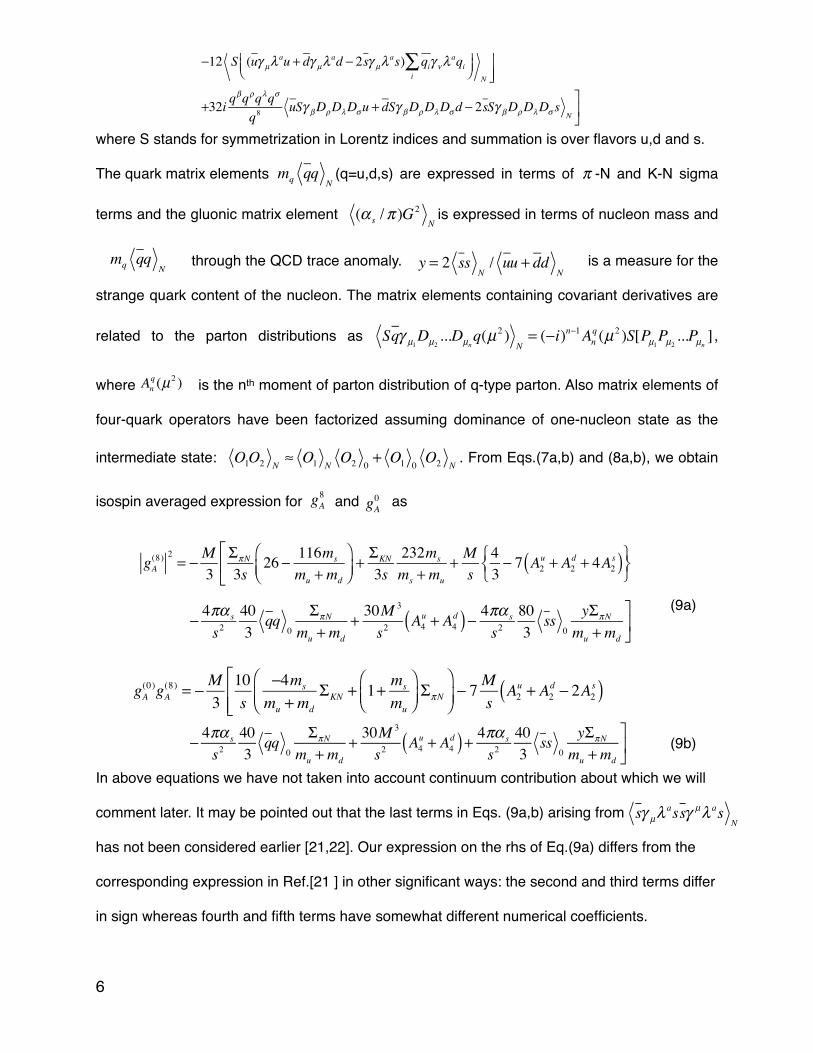
where S stands for symmetrization in Lorentz indices and summation is over flavors u,d and s.!

The quark matrix elements ! ! (q=u,d,s) are expressed in terms of � -N and K-N sigma

terms and the gluonic matrix element � is expressed in terms of nucleon mass and

! ! through the QCD trace anomaly. is a measure for the

strange quark content of the nucleon. The matrix elements containing covariant derivatives are

related to the parton distributions as � ,

where is the nth moment of parton distribution of q-type parton. Also matrix elements of

four-quark operators have been factorized assuming dominance of one-nucleon state as the

intermediate state: � . From Eqs.(7a,b) and (8a,b), we obtain

isospin averaged expression for and as!

!! ! ! ! ! ! ! ! ! ! ! ! ! (9a)!

!!!! ! ! ! ! ! (9b)!

In above equations we have not taken into account continuum contribution about which we will

comment later. It may be pointed out that the last terms in Eqs. (9a,b) arising from

has not been considered earlier [21,22]. Our expression on the rhs of Eq.(9a) differs from the

corresponding expression in Ref.[21 ] in other significant ways: the second and third terms differ

in sign whereas fourth and fifth terms have somewhat different numerical coefficients. ! ! !

π

(α s /π )G2

N

Sqγ µ1Dµ2...Dµn

q(µ2 )N= (−i)n−1An

q (µ2 )S[Pµ1Pµ2 ...Pµn ]

O1O2 N ≈ O1 N O2 0 + O1 0 O2 N

�6

−12 S (uγ µλau + dγ µλ

ad − 2sγ µλas) qi

i∑ γ νλ

aqi⎛⎝⎜

⎞⎠⎟

N

⎤

⎦⎥⎥

+32i qβqρqλqσ

q8uSγ βDρDλDσu + dSγ βDρDλDσd − 2sSγ βDρDλDσ s N

⎤

⎦⎥

mq qqN

mq qqN

Anq (µ2 )

gA8 gA

0

gA(8) 2 = − M

3ΣπN

3s26 − 116ms

mu +md

⎛⎝⎜

⎞⎠⎟

⎡

⎣⎢ + ΣKN

3s232ms

ms +mu

+ Ms

43− 7 A2

u + A2d + 4A2

s( )⎧⎨⎩

⎫⎬⎭

− 4πα s

s2403

qq0

ΣπN

mu +md

+ 30M3

s2A4u + A4

d( )− 4πα s

s2803

ss0

yΣπN

mu +md

⎤

⎦⎥

gA(0)gA

(8) = − M310s

−4ms

mu +md

ΣKN + 1+ ms

mu

⎛⎝⎜

⎞⎠⎟ΣπN

⎛

⎝⎜⎞

⎠⎟⎡

⎣⎢⎢

− 7Ms

A2u + A2

d − 2A2s( )

− 4πα s

s2403

qq0

ΣπN

mu +md

+ 30M3

s2A4u + A4

d( )+ 4πα s

s2403

ss0

yΣπN

mu +md

⎤

⎦⎥

sγ µλassγ µλ as

N

y = 2 ssN/ uu + dd

N

!

3. Results and Discussion!

In the current literature, there are significant variations in the values of the QCD and hadronic

parameters appearing in Eqs. (9a) and (9b). The most important parameters are the second

moments of the parton distributions. For calculating , we have used MSTW 2008

parametrization of parton distributions at � [25]. This gives !

! ! and ! . These authors have also used NNLO parametrization of

strong coupling constant at � as � =0.45077 whereas it is common to use �

=0.5 in QCD sum rule calculations [23,24]. For 2+1 flavors from lattice QCD world data, Alvarez-

Ruso et al.[26] have determined � . For K-N

sigma term , Nowak, Rho and Zahed [13] estimate

� for y=0, 0.1 and 0.2 with � and !

! . . Actually, for the strange quark content of the nucleon, the lattice result for y is

considered more accurate than sigma-term and is given as y=0.135(22)(33)(22)(9) [27]. For

current quark masses at � , Ioffe et al. [28] have obtained assuming!

! ! and! ! ! ! whereas! ! ! ! in

Ref.[29]. For light quark vacuum condensate ! ! ,value for between

0.45 GeV3 to 0.65 GeV3 has been commonly used [23,24,28].!

! In view of this prevailing uncertainty in numerical values of these parameters, it is

desirable to take these uncertainties into account while determining the axial coupling constants

of the nucleon from Eqs. (9a,b). We will vary each of these parameters by (10-20)% of their

certain central values covering roughly their ranges as given above with an aim to obtain values

of axial coupling constants of the nucleon as determined by experiments and phenomenological

µ = 1GeV

µ = 1GeV α s (µ) α s (µ)

ΣπN = 12(mu +md ) uu

N+ dd

N( ) = 52(3)(8)MeV

ΣKN ≈ (2.3,2.8,3.4)mπ mq =12(mu +md ) = 5MeV ,ms = 135MeV

µ = 1GeV

�7

Anq (µ2 )

A2u + A2

d = 0.9724,A2s = 0.0479,

A4u + A4

d = 0.1206 A4s = 0.0011

ΣKN = 12(mq +ms ) uu

N+ ss N( )

ΣπN = 45MeV

mu +md = 10.0 ± 2.5MeV

ms ≈147MeV

ms (2GeV ) = 120MeV , mu +md = 12.8 ± 2.5MeV

qq0= uu

0= dd

0(2π )2 qq

0

analyses. In addition to this, we also chose ! ! ! [28] , and ! from MSTW

2008 [25]. We observed that the sum rules were giving unphysical results for and for

Borel mass squared ! and reasonable results are obtained for ! for various

combinations of QCD and hadronic parameters. We seek stable results for and in the

range . For this, we first varied ! ! ! ! ! ! !

and y by ~(10-20)% around a central value of each of these parameters as given in the second

row of Table 1. First we found those sets of parameters for which ! ! is obtained

from Eq.(9a) for ! ! ! . These parameter sets were further constrained by

requiring that! at the middle of the Borel mass parameter range, i.e. at ! , lies in

the range 0.29-0.42. Among these sets of parameters, we looked for those which were giving

most stable results for and against variation of Borel mass squared parameter s.

Actually, and y are not independent parameters and are related as ! !

! . We found that for a given set of ! and , if ! and y are chosen

according to this relation then the sum rules do not work well. Hence we have varied! and y

independently while y has been used only in the last terms of Eqs.(9a) and (9b). However, we

have tried to keep ! and ! as close as possible and maintained ! to be in the range

of (82-85)% of . In Table 1, only those results are displayed for which and ! are

closest possible for a given set of and ! . We may consider this use of independent

values for and y or as a way to compensate the possible violation of factorization

hypothesis used in the last terms of Eqs. (9a) and (9b). We get a wide range of combination of

parameters! ! ! ! ! ! and y being used in the current

literature for which the sum rules give values of ! and which lie in the typical range that

is obtained from experimental and phenomenological analyses. We believe this as a sign of

robustness of our sum rules. In Table 1 we have listed some of those results for which !

�8

ss0= 0.8 qq

0 A2s = 0.048

gA8 gA

0

s ≤1.3GeV 2 s ≥1.6GeV 2

gA8 gA

0

1.7GeV 2 ≤ s ≤ 2.5GeV 2 ms ,mq ,ΣπN ,ΣKN , qq 0,α s ,A2

u + A2d ,A4

u + A4d

1.7GeV 2 ≤ s ≤ 2.5GeV 2

0.52 < gA8 < 0.64

gA0 s = 2.1GeV 2

gA8 gA

0

ΣKN ΣKN (y) =14(1+ y)×

1+ ms

mq

⎛

⎝⎜⎞

⎠⎟ΣπN ms ,mq ΣπN ΣKN

ΣKN

ΣKN ΣKN (y) ΣKN

ΣKN (y) ΣKN ΣKN (y)

ms ,mq ΣπN

ΣKN

ms ,mq ,ΣπN ,ΣKN , qq 0,α s ,A2

u + A2d ,A4

u + A4d

gA8 gA

0

ΣKN (y)

, as a function of s, has minimum slopes in our designated interval s= (1.7-2.5) GeV2. Plots

of some of these results are displayed in Figs. (1-6). We observe from the Table 1 that! !

was stuck to the lower end of the range of its variation and ! was confined to (300-325)

MeV. The best results were obtained for y being in the range (0.16 - 0.18).!

As in any QCD sum rule calculation, our results have errors due to omission of contributions

of higher dimensional operators and continuum contributions. From MSTW 2008 parametriz-

ation [25], we estimate ! ! ! ! and ! ! ! ! .

The ratio of contributions of six-dimensional operators to that of four-dimensional operators is

~1/2 at s=2.5 GeV2, but the ratio of contribution of eight-dimensional operators to! that of four-

dimensional operator is likely to be few percent, though their contribution to ! will get

doubled on account of sign difference in the contributions of four-dimensional and six-

dimensional operators. The continuum contribution comes from and states. A

rough estimate shows that their contribution will be less than 1%. Thus we allow the error due to

exclusion of contributions of higher dimensional operators and continuum contributions to be

roughly 10%. Based on results given in Table 1 and the error estimates, we conclude !

! ! ! ! ! ! ! ! ! ! ! ! (10a)!

! ! ! ! ! ! ! ! ! ! ! ! (10b)! !

where the first error is due to finite slope within the designated range of Borel mass parameter

and the second one is due to omission of contributions of higher dimensional operators and

continuum contribution. !

By choosing the correlator of singlet and octet axial-vector currents, we ensured that the

disconnected diagrams do not contribute directly for determination of . However, the non-

valence components in the nucleon, such as strange quark-antiquarks and gluons, have an

important role: they are directly responsible for the splitting of and . In QCD parton model,

the axial coupling constants of a nucleon are related to polarized quark densities. Our results for !

�9

gA0

A2u + A2

d

ΣKN

A3u + A3

d ! 0.3,A6u + A6

d ! 0.03 (A3u + A3

d ) qq0! 3.8 ×10−3GeV 3

gA8,0

η − N η '− N

gA8 = 0.59 ± 0.05 ± 0.06

gA0 = 0.39 ± 0.05 ± 0.04

gA0

gA8

gA0

and implies that polarized s-quark density is negative: . A numerical analysis of

Eqs. (8a-9b) shows that gets contribution from and . While the

first two quantities make negative with giving dominant contribution, the last two

quantities contribute positively with the gluon contribution being dominant one. The use of four

s-quark operators and its subsequent evaluation in the form of term by factorization

hypothesis gives a semblance of “disconnected” diagram contributing to sum rules. However,

this contribution is the smallest one. We can also look at the problem of negative using the

generalized GT relation [7]. Realizing that , we can define its decay

constants as and estimate ! ! and ! ! from !

[23,24]. Also from =(3 - 5) [30] and =(1 - 2) [7], and on using U(1)A GT relation

for s-quark only gives !! ! .! !

!4. Conclusion! !

By considering the correlation function of octet-octet and octet-singlet axial-vector currents

between one-nucleon states, we have obtained sum rules for ! and! without use of

instantons. For numerical evaluation of and , we use sets of QCD and hadronic

parameters which appear in our sum rules such that they lie in a range which has been obtained

from phenomenological and theoretical analyses in recent years. We found that there exists a

large number of such parameter sets which can yield and ! that lie within a range which

is consistent with the current determination of their values from experimental and

phenomenological analyses. Basically, we chose QCD and hadronic parameter sets which yield,

through our sum rules, values of ! , in a chosen interval of Borel mass parameter, in a range

which is phenomenologically acceptable. We further restricted these sets of parameters so that

the values of at the middle of the Borel mass squared parameter interval lie in a range

which is currently acceptable from experimental data combined with theoretical QCD analysis.

�10

gA8 2 gA

0gA8

gA8 gA

0

gA8 gA

0

gA8

gA0

gA8 gA

0 Δs ∼ −0.08

Δs ssN,A2

s , α s

πG2

N

ss0y

Δs A2s

ss0y

Δs

sγ µγ 5s = ( jµ50 − 2 jµ5

8 ) / 3

0 sγ µγ 5s η(') (p) = ipµ fη(')

s fηs ! −124.2MeV fη '

s ! 115.0MeV

fη(')0,8 gηNN gη 'NN

−Δs ! (0.09 − 0.16)

We accept ! obtained in the entire designated interval of Borel mass parameter as our final

result of sum rules. We also note an interesting point that the sign of spin-dependent parton

density is decided by spin-independent quantities such as second moment of spin-

independent parton distribution function of s-type and s-quark content of the nucleon. In

conclusion, the present method of QCD sum rule, where correlation function of two axial-vector

currents between one-nucleon states is studied, is capable of producing a result for singlet

axial-vector coupling constant of the nucleon which is consistent with its current determination

from experiments and QCD theoretical analysis. !

!ACKNOWLEDGEMENT : The author thanks Department of Science & Technology, Government

of India, for financial support.!

!References!

[1] C. A. Aidala,S. D. Bass, D. Hasch and G. K. Mallot, Rev. Mod. Phys. 85 (2013) 655.![2] S. D. Bass, Mod. Phys. Lett. A 24 (2009) 1087.![3] A. W. Thomas, A. Casey and H. H. Matevosyan, Int. J. Mod. Phys. A 25 (2010) 4149.![4] S. D. Bass and A. W. Thomas, Phys. Lett. B 684 (2010) 216.![5] A. V. Efremov, J. Soffer and N. A. Tornqvist, Phys. Lett. B 64 (1990) 1495.![6] S. Narison, G. M. Shore and G. Veneziano, Nucl. Phys. B 546 (1999) 235.![7] G. M. Shore, Nucl. Phys. B 744 (2006) 34.![8] J. Beringer et al. (Particle Data Group), Phys.Rev. D 86 (2012) 010001. ![9] F. E. Close and R. G. Roberts, Phys. Lett. B 316 (1993) 165.![10] M. E. Carrillo-Serrano, Phys. Rev. C 90 (2014) 064316.![11] E. Leader and D. B. Stamenov, Phys. Rev. D 67 (2003) 037503.![12] V. Y. Alexakhin et al. (COMPASS Collab.), Phys. Lett. B 647 (2007) 8.![13] M. A. Nowak, M. Rho and I. Zahed, “Chiral Nuclear Dynamics”, World Scientific, Singapore ! (1996). ![14] T. Schafer and V. Zetocha, Phys. Rev. D 69 (2004) 094028.![15] Y. B. Yang et al., arXiv 1504.04052 (hep-lat). ![16] H. Dahiya and M. Randhawa, Phys. Rev. D 90 (2014) 074001.![17] P. E. Shanahan et al., Phys. Rev. Lett. 110 (2013) 202001.![18] A. J. Buchmann and E. M. Henley, Phys. Rev. D 83 (2011) 096011.![19] B. L. Ioffe and A. G. Oganesian, Phys.Rev. D 57 (1998) R6590.![20] A. V. Belitsky and O.V. Teryaev, Phys. Lett. B 366 (1996) 345.![21] T. Nishikawa, S. Saito and Y. Kondo, Phys. Rev. Lett. 84 (2000) 2326.![22] T. Nishikawa, Phys. Lett. B 597 (2004) 173.!

�11

gA0

Δs

[23] J. P. Singh and J. Pasupathy, Phys. Rev. D 79 (2009) 116005.![24] J. P. Singh, Phys. Rev. D 88 (2013) 096005.![25] A. D. Martin, W. J. Stirling, R.S. Thorne and G. Watt, arXiv 0901.0002 (hep-ph).![26] L. Alvarez-Ruso et al., arXiv 1402.3991 (hep-lat).![27] C. Alexandrou, arXiv: 1404.5213 (hep-lat).![28] B. L.Ioffe, V. S. Fadin and L. N. Lipatov, “Quantum Chromodynamics: Perturbative and ! Nonperturbative Aspects”, Cambridge University Press (2010). ![29] J. Prades, Nuc. Phys. B 64 (Proc. Suppl.) (1998) 253. ![30] J. P.Singh, F. X. Lee and L.Wang, Int. J. Mod. Phys. A 26 (2011) 947.!!!

!

Table 1: Our results for and ! for s= 1.7 GeV2 and 2.5 GeV2 with low slopes in s. ! = !! ! . ! ! and! are in MeV and ! ! is in GeV3. In the second row, the range of variation of the parameters appearing in the first row is shown.!

mq y

0.13-0.20

135-155

45-!60

250-400

0.45-0.60

0.45-0.50

0.95-1.00

0.11-0.13

5-7

0.16 155 57.5 325 0.45 0.475 0.95 0.12 7 0.579 0.639 0.344 0.441 0.098

0.16 155 57.5 325 0.475 0.45 0.95 0.12 7 0.579 0.639 0.344 0.441 0.098

0.17 135 52.5 300 0.45 0.50 0.95 0.11 6 0.558 0.634 0.341 0.440 0.099

0.17 135 52.5 300 0.475 0.475 0.95 0.11 6 0.557 0.633 0.340 0.440 0.100

0.17 135 52.5 300 0.50 0.45 0.95 0.11 6 0.558 0.634 0.341 0.440 0.099

0.17 150 55.0 300 0.55 0.45 0.95 0.11 7 0.560 0.633 0.341 0.439 0.098

0.17 150 55.0 300 0.50 0.50 0.95 0.11 7 0.555 0.631 0.337 0.438 0.101

0.17 155 57.5 325 0.45 0.45 0.95 0.13 7 0.573 0.637 0.338 0.439 0.101

0.18 150 47.5 300 0.50 0.475 0.95 0.12 6 0.562 0.637 0.340 0.441 0.100

0.18 150 47.5 300 0.525 0.45 0.95 0.12 6 0.565 0.639 0.342 0.441 0.099

0.18 150 47.5 300 0.475 0.50 0.95 0.12 6 0.562 0.637 0.340 0.441 0.100

0.18 150 47.5 300 0.575 0.45 0.95 0.11 6 0.542 0.629 0.342 0.442 0.100

0.20 135 52.5 300 0.45 0.45 0.95 0.13 6 0.544 0.628 0.341 0.441 0.099

0.20 150 55.0 300 0.45 0.50 0.95 0.13 7 0.540 0.626 0.337 0.438 0.101

0.20 150 55.0 300 0.50 0.45 0.95 0.13 7 0.540 0.626 0.337 0.438 0.101

�12

ΔgA0− qq (2π )2 α sΣKNΣπN

ms A2u + A2

d A4u + A4

d gA8 (2.5)gA

8 (1.7) gA0 (2.5)gA

0 (1.7)

gA8 gA

0

ΔgA0 mq ,ms ,ΣπN ΣKN − qq (2π )2gA

0 (2.5) − gA0 (1.7)

!

!

!!!!

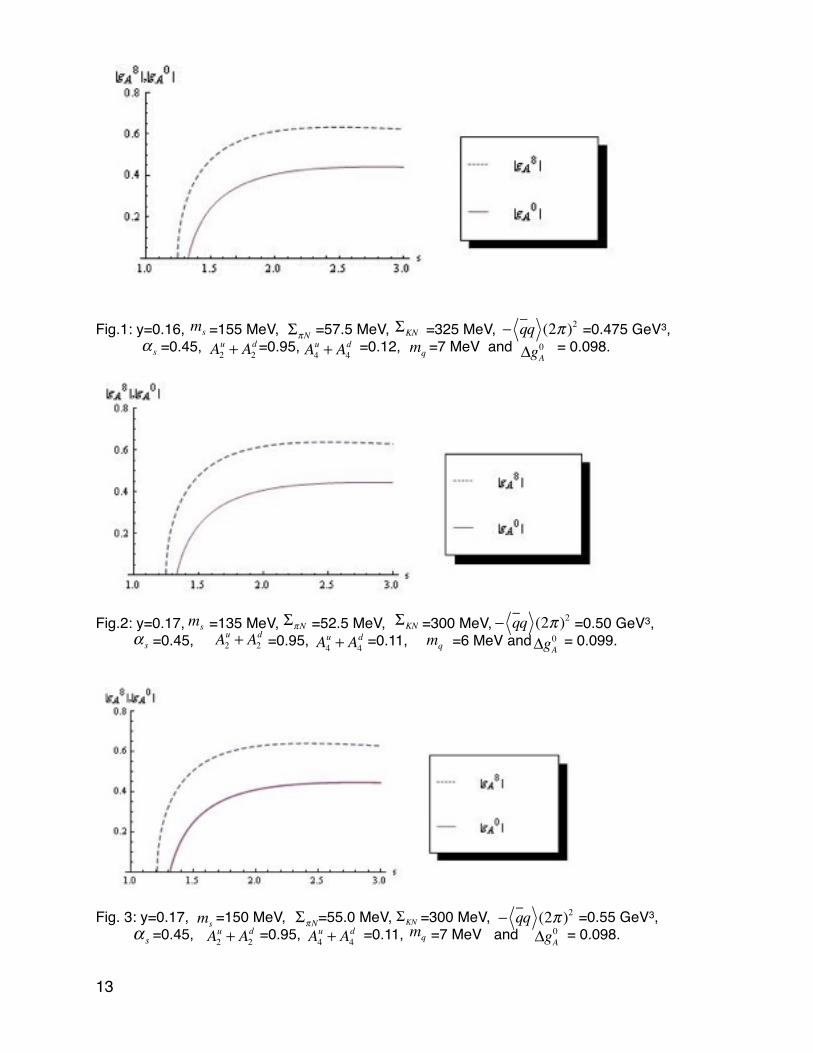
!Fig.1: y=0.16, =155 MeV, =57.5 MeV, =325 MeV, ! ! =0.475 GeV3, ! =0.45, =0.95, ! =0.12, =7 MeV and = 0.098.!!!!!!!!

!

Fig.2: y=0.17, =135 MeV, ! =52.5 MeV, =300 MeV, ! ! =0.50 GeV3, ! =0.45, ! =0.95, ! =0.11, =6 MeV and = 0.099.!!

!!!!!!!!Fig. 3: y=0.17,! =150 MeV, =55.0 MeV, =300 MeV, ! ! =0.55 GeV3, ! =0.45, ! =0.95, ! =0.11, ! =7 MeV and = 0.098.!

�13

mqA4u + A4

d− qq (2π )2

α s A2u + A2

dΣKNms ΣπN

ΣKNms − qq (2π )2α s A2

u + A2d

ΣπN

A4u + A4

d mq

− qq (2π )2ΣπN ΣKN

A4u + A4

dA2u + A2

d mqα s

ms

ΔgA0

ΔgA0

ΔgA0

!!

!!!!! !

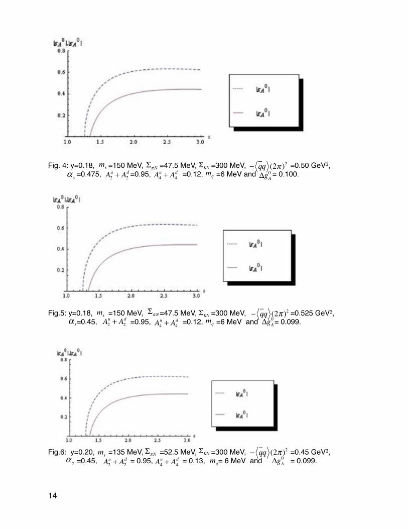
Fig. 4: y=0.18,! =150 MeV, =47.5 MeV, =300 MeV, ! ! =0.50 GeV3, ! =0.475, ! =0.95, ! =0.12, ! =6 MeV and = 0.100.!!!!!!!!!

!Fig.5: y=0.18,! =150 MeV, =47.5 MeV, =300 MeV, ! ! =0.525 GeV3, ! =0.45, ! =0.95, ! =0.12, ! =6 MeV and = 0.099.!!

!!!!!

!

Fig.6: y=0.20,! =135 MeV, =52.5 MeV, =300 MeV, ! ! =0.45 GeV3, ! =0.45, ! = 0.95, ! = 0.13, ! = 6 MeV and ! = 0.099.!

�14

− qq (2π )2ΣπN ΣKN

A4u + A4

dA2u + A2

d mqα s

ms

msA2u + A2

dα s mq

− qq (2π )2ΣKN

A4u + A4

dΣπN

msmqA2

u + A2d

− qq (2π )2ΣπN ΣKN

A4u + A4

dα s

ΔgA0

ΔgA0

ΔgA0