SINGAPORE MANAGEMENT UNIVERSITY

School of Economics

Econ107 Introduction to Econometrics

Sample Questions

(Time allowed: 2 hours)

1 Consider the 2 variable regression model

iii XY 10 (1)

Denote 1̂ to be the OLS estimator of 1 and )ˆ( 1se to be

2

2ˆ

ix

.

For each of the following statements indicate whether it is justified and explain

your reasons.

(a) Multicollinearity raises the standard error of 1̂ and hence the t-test based on

1̂ and )ˆ( 1se is invalid. (6 marks)

(b) Heteroskedasticity leads to an unbiased estimator of 1̂ and hence the t-test

based on 1̂ and )ˆ( 1se is valid. (6 marks)

(c) Serial correlation leads to an unbiased estimator of 1̂ but the t-test based on

1̂ is always invalid. (6 marks)

(d) Misspecification of the functional form leads to an unbiased estimator of

1̂ but the t-test based on 1̂ and )ˆ( 1se is invalid. (6 marks)

(e) If iY is a dummy variable, the linear probability model allows for an

unrestricted range of probability, hence the t-test based on 1̂ is always

invalid. (6 marks)

2. Suppose you are given the following results for a time series of 23 annual

Australian aggregate economic data (standard errors in parentheses):

)09.1()66.0()95.0()91.8(

121.0452.095.0133.8ˆ4apwC ttt

………(1)

95.02 R

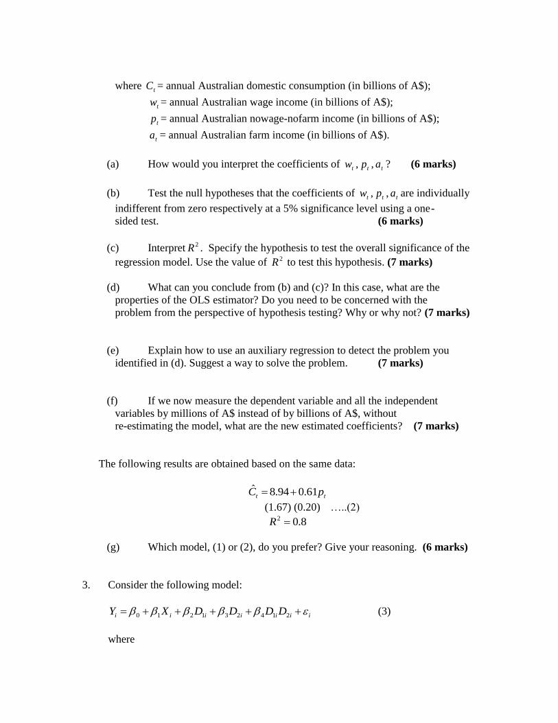
where tC = annual Australian domestic consumption (in billions of A$);

tw = annual Australian wage income (in billions of A$);

tp = annual Australian nowage-nofarm income (in billions of A$);

ta = annual Australian farm income (in billions of A$).

(a) How would you interpret the coefficients of tw , tp , ta ? (6 marks)

(b) Test the null hypotheses that the coefficients of tw , tp , ta are individually

indifferent from zero respectively at a 5% significance level using a one-

sided test. (6 marks)

(c) Interpret 2R . Specify the hypothesis to test the overall significance of the

regression model. Use the value of 2R to test this hypothesis. (7 marks)

(d) What can you conclude from (b) and (c)? In this case, what are the

properties of the OLS estimator? Do you need to be concerned with the

problem from the perspective of hypothesis testing? Why or why not? (7 marks)

(e) Explain how to use an auxiliary regression to detect the problem you

identified in (d). Suggest a way to solve the problem. (7 marks)

(f) If we now measure the dependent variable and all the independent

variables by millions of A$ instead of by billions of A$, without

re-estimating the model, what are the new estimated coefficients? (7 marks)

The following results are obtained based on the same data:

tt pC 61.094.8ˆ

(1.67) (0.20) …..(2)

8.02 R

(g) Which model, (1) or (2), do you prefer? Give your reasoning. (6 marks)

3. Consider the following model:

iiiiiii DDDDXY 214231210 (3)

where

Y = annual salary of a junior college teacher (in thousand S$)

X = years of teaching experience

iD1 = 0 if female

= 1 otherwise

iD2 = 0 if non-Chinese

= 1 otherwise

(a) The term ii DD 21 represents the interaction effect. Is this term a dummy

variable? If so, what does this term means? (4 marks)

(b) Show how equation (3) can be used to find the mean salary for a non-Chinese

female. (2 marks)

(c) Show how equation (3) can be used to find the mean salary for a Chinese

female. (2 marks)

(d) Show how equation (3) can be used to find the mean salary for a non-Chinese

male. (2 marks)

(e) Show how equation (3) can be used to find the mean salary for a Chinese

male. (2 marks)

(f) Using the results obtained from (b)-(e) to interpret 4 . (5 marks)

Eviews is used to produce the following regression results (with four t-statistics, one

standard error and one p-value removed) based on cross-sectional data on 1000 junior

college teachers in Singapore:

Dependent Variable: Y Method: Least Squares Date: 10/25/05 Time: 11:40 Sample: 1 1000 Included observations: 1000

Variable Coefficient Std. Error t-Statistic Prob.

C 32.0 4.0 A1 0.000 X 1.2 0.2 A2 0.000

D1 2.326 1.0 A3 A6 D2 1.645 1.0 A4 0.10

D1*D2 0.65 A5 6.5 0.000

R-squared 0.686082 Mean dependent var 103.7238 Adjusted R-squared 0.684820 S.D. dependent var 8.951610 S.E. of regression 5.025510 Akaike info criterion 6.071918 Sum squared resid 25129.47 Schwarz criterion 6.096457 Log likelihood -3030.959 F-statistic 543.6556 Durbin-Watson stat 2.060918 Prob(F-statistic) 0.000000

(g) Find the numerical values for A1-A6 in the above Eviews output.

(4 marks)

(h) Construct the 95% confidence interval for the slope parameter of X and

interpret it. (4 marks)

(i) If we now measure Y by S$ instead of by thousands of S$, without

rerunning the regression, what are the new estimated coefficients?

(5 marks)

Selected Formulae

- 1 =)] se(t + )se(t - Prob[

)]n[Var(-1

n )

2

d - (1 h

)K - (n / )R - (1

/K R = F

nTSS

KnRSSR

TSS

ESS = R

RSS + ESS = TSS x

= )se(

x n

X = ) se(

K - n

e =

X + = Y Xn - X

YXn - Y X =

x

y x =

x = y X - X = x Y - Y = y

/2/2

2

2

2

2i

2i

2i

22i

22i

ii

2i

ii

iiiiii

ˆˆˆˆ

ˆ

1

,)1/(

)1/(1,

ˆˆ

ˆˆ1

ˆ

ˆˆ,ˆ

ˆˆ

11111

2

1

0

101

1

Selected Statistical Tables

1. Table for the Normal distribution.

2. Table for the t distribution.

3. Table for the F distribution

4. Table for the Durbin-Watson test statistic.