A Unified Test for Substantive and Statistical Significance in

Political Science

Justin H. GrossUniversity of North Carolina at Chapel Hill

Department of Political Science

jhgross@unc.edu

May 31, 2013

Abstract

For over a half-century, various fields in the behavioral and social sciences have debated the

appropriateness of null hypothesis significance testing (NHST) in the presentation and assess-

ment of research results. A long list of criticisms have fueled a recurring “significance testing

controversy” that has ebbed and flowed in intensity since the 1950s. The most salient problem

presented by the NHST framework is that it encourages researchers to devote excessive atten-

tion to statistical significance while underemphasizing substantive (scientific, contextual, social

political, etc.) significance. What might best serve as a diagnostic tool for distinguishing signal

from noise continues to be mistaken, far too often, as the primary result of interest. Our fore-

most goal in analyzing data ought to be ascertaining the other type of significance, measuring

and interpreting relevant magnitudes. I introduce a simple technique for giving simultaneous

consideration to both forms of significance via a unified significance test (UST). This allows the

political scientist to test for actual significance, taking into account both sampling error and an

assessment of what parameter values should be deemed interesting, given theory.

1 Introduction

It may or may not come as a surprise that many scientists agree with Meehl (1978) that

“excessive reliance on significance testing is a poor way of doing science,” leading to theories

that “lack the cumulative character of scientific knowledge, . . . [tending] neither to be refuted nor

corroborated, but instead merely fad[ing] away as people lose interest.” Meehl’s insistence that

1

“the almost universal reliance on merely refuting the null hypothesis as the standard method for

corroborating substantive theories in [certain areas of psychology] is a terrible mistake, basically

unsound, . . . and one of the worst things that ever happened in the history of psychology” (p.817,

my emphasis) may seem an exaggeration, but to the extent that social and behavioral sciences

fetishize the rejection of point null hypotheses, instilling the practice with importance out of all

proportion to its true contribution, the spirit of the statement is apt. What is at issue is not the

scientific practice of generating hypotheses from theory, then utilizing data as evidence in sorting

through these hypotheses. Rather, it is the peculiar way this typically plays out in practice that

falls well short of what science requires.

More than fifteen years have has passed since a group of psychologists imagined: “What if

there were no significance tests?” in their edited volume of the same name (Harlow, Mulaik and

Steiger, 1997). Their rhetorical query may as well have been a flight of fancy on the order of

John Lennon’s entreaty to “imagine no possessions.” A more modest, realistic, question might

be posed: What if significance tests were more meaningful, more, well. . . significant. Regardless

of one’s philosophical perspective on statistical inference (i.e., even if one is unwilling to stray

from a conservative frequentist interpretation of probability), it is possible to do much better

than reflexively reporting statistical significance, signs, and p-values, and making these the focus

of discussion. We have become deeply accustomed to declarations of statistical significance and

asterisks next to parameter estimates and, while such rituals are regularly misconstrued or distract

from more meaningful conversation about the data, may play a role in communicating simple

summaries of findings. After all, we ideally write for more than one audience, wishing to reach

scientist and layperson alike, and even scientific audiences will approach di↵erent studies with

di↵erent purposes, often wishing to start with a cursory yet meaningful look at results. As it

stands, much of the resistance to simply banishing p-values and tabular asterisks altogether is

motivated not by laziness, not from a desire to have authors spoon-feed us results, as more cynical

critics may charge, but from a desire for commonly accepted heuristics in assessing research results.

The problem is that p-values and asterisks aren’t quite suited to the task. Moreover, rather than

serving as an invitation to the reader to delve more deeply into the substantively meaningful results,

2

secure in the knowledge that apparent patterns are not likely attributable to sampling error, these

heuristics are often o↵ered and accepted as a substitute for interpretation of magnitudes in context,

an end rather than a beginning to the conversation.

In what follows, I propose a simple way to integrate statistical and substantive (a.k.a. scientific,

contextual, social, political, economic, or real-world) significance, in the hope that this may restore

some balance to analyses that have dwelled too heavily on the former. At the very least, I hope

to encourage political scientists to join a conversation that has been prominent in the social and

behavioral sciences generally and yet nearly absent from political science, beyond a few notable

recent exceptions (Gill, 1999; Ward, Greenhill and Bakke, 2010; Esarey, 2010).

In Section 2, I briefly review the the most damning criticisms of null hypothesis significance

testing (NHST), noting that the manner in which it is conventionally applied in political science

serves as a distraction from—or poor substitute for—close interpretation of results. In Section 3, I

propose a simple solution, in the form of a unified statistical and substantive significance test (UST)

that overcomes the most troubling shortcomings of NHST. In Section 4, I conclude by suggesting

that we pay attention to the some recent developments in other fields, such as informative hypothesis

testing and minimal important di↵erences within health outcomes research for tools that may serve

us in more carefully setting up reasonable statistical hypotheses and justifying the conclusions we

draw from the data we have.

2 The Controversy that Passed Us By: Debating the Merits of

NHST

The function of statistical tests is merely to answer: Is the variation great enoughfor us to place some confidence in the result; or, contrarily, may the latter be merelya happenstance of the specific sample on which the test was made? The questionis interesting, but it is surely secondary, auxiliary, to the main question: Does theresult show a relationship which is of substantive interest because of its nature andits magnitude? Better still: Is the result consistent with an assumed relationship ofsubstantive interest? (Kish (1959), reprinted in Morrison and Henkel (1970), emphasisKish’s)

Some time ago, I attended a talk by a political scientist who was doing some research on teacher

3

training. After explaining his research design, in which teacher success would be operationalized

using students’ scores on standardized exams, he presented a slide with a long list of coe�cients

estimated under several models, o↵ering the standard apology for the vast sea of numbers. To wade

through the slide, in keeping with ritual, he called our attention to one or two variables, which,

like Dr. Seuss’s star-bellied Sneetches, had enough good fortune to be marked by the asterisks its

companions were lacking. He then noted that, according to his results, parents might do well to ask

whether their children’s teachers received in-state training. For, after controlling for a long list of

other predictors, the estimated “e↵ect” of in-state training was found to be positive and statistically

significant. Asked about units, the presenter could only say that the scores were based on some

composite standardized measure, but not how the numbers ought to be interpreted. As it turned

out, the expected jump in test scores associated with a teacher being trained in-state was around

one-fortieth of a standard deviation! Pressed on whether a parent should seriously be concerned

by a (predicted) relationship so small, he conceded that the magnitude did not seem too large, but

it was statistically significant, after all. This extreme deference to statistical significance, wherein

the very term “statistical” is lorded over the audience as if to imply that it is but a more rigorous

form of everyday significance, leads to opportunities for mischief and – even more perniciously –

rewards laziness.

At various points over the past half century or so, individual fields in the behavioral, health, and

social sciences have grappled publicly with the issue of what role significance testing of hypotheses

should take in the assessment of research results. Psychology, sociology and economics have devoted

volumes to the topic, special issues of journals as forums for debating the various dimensions of the

“controversy,” and even argued over whether policies for publication ought to be changed to reflect

the limitations of conventional hypothesis testing (Morrison and Henkel, 1970; Harlow, Mulaik and

Steiger, 1997; Altman, 2004).1

1The history of the controversies surrounding the so-called null hypothesis significance testing procedure hastypically been traced to passionate disagreements between the towering figures of early twentieth century statistics,Sir R.A. Fisher on one hand and J. Neyman and E.S. Pearson on the other. A thorough historical treatment ofstatistical significance and the roles of Fisher, Neyman and Pearson is provided by Gigerenzer, Swijtink and Daston(1990, p. 79–109), with other good summaries found in Gill (1999) and Ziliak and McCloskey (2008). Fisher is oftencredited with giving us the notion of statistical significance, and indeed he emphasized it in his work and bears muchof the responsibility for its eventual dominance, but the notion did not originate with him. In fact, some version of itappeared some two hundred years prior (Arbuthnot, 1710), though its role would be quite minor until Fisher’s work

4

There is, frankly, much to dislike about the NHST approach to social science, and these have

been outlined comprehensively elsewhere (see, for example, Cohen (1994); Gill (1999); Ziliak and

McCloskey (2008)). A few of the most troubling aspects of NHST are next discussed in brief.

Levels of significance are arbitrary and p-values misunderstood.

The basic strategy of using the tail area of the null distribution—the probability, under H0,

of observing a test statistic more extreme than the actual one—originated in an earlier test for

identifying outliers (see an account in Gigerenzer, Swijtink and Daston (1990)). Critics often note

the awkwardness of even the correct interpretation of p-values; according to the oft-repeated quip

of Je↵reys, “What the use of P implies is that a hypothesis that may be true may be rejected

because it has not predicted observable results that have not occurred” (Je↵reys, 1961). Indeed the

typical manner in which social and behavioral scientists report statistical significance is an even less

satisfactory compromise; two to four conventional choices for significance level ↵ are considered,

and superscripts are placed on the parameter estimates to indicate the lowest such ↵ at which H0

would be rejected if we were to conduct a decision-oriented hypothesis test.

Unfortunately, as Gelman and Stern (2006) put it in the title of their article, “the di↵erence

between ‘significant’ and ‘not significant’ is not itself statistically significant.” Under the dominant

contemporary approach to hypothesis testing in social science, one is presumed to make a dis-

crete decision to either reject the null hypothesis in favor of the alternative or to fail to reject it.

Choosing the significance level ↵ in advance allows one to limit the probability of rejecting the null

should it in fact be true. The p-value, or “attained significance level,” from the perspective of this

approach, does not o↵er a measure of how significant the finding is, but might rather be considered

a form of sensitivity analysis, allowing one to assess whether the result is robust to the arbitrary

choice of ↵. And yet, we too commonly imbue p-values with qualitative meaning that is utterly

unjustified. Even textbooks sometimes reinforce this misunderstanding; for example, one popular

book would have readers interpret p-values as indicating that a result is “extremely significant,”

and popularization of his approach. A hybrid of Fisher’s “significance tests” and Neyman-Pearson “hypothesis tests”would come to be codified in a number of mid-twentieth-century teaching texts, and it is this approach, commonlyreferred to as “null hypothesis significance testing,” that dominates common practice in the social and behavioralsciences.

5

“highly significant,” “statistically significant,” “somewhat significant,” “could be significant,” or

“not significant” based on the interval in which it lies (Verzani, 2005). Even worse, this particular

set of criteria seems to imply that if a p-value is small enough (less than 0.01), it somehow implies

scientific significance, while p-values in the interval (0.01, 0.05] are indicative of results that are

only statistically significant.

The typical misrepresentation of p-values is less grotesque, involving an inversion of conditional

probabilities. We seem to be constitutionally incapable of not treating Pr(data|H0) as Pr(H0|data).

When told that the latter expression is meaningless within a frequentist framework—with no way

to assign probabilities to hypotheses unless we take a Bayesian approach—we grasp at the former

as the closest substitute for what we seek.

One reason we so readily accept the inverted conditional probability as a substitute is the

incorrect perception that modus tollens reasoning applies to probabilistic statements. In deductive

logic, argument by contrapositive is always permissible: “If A, then B ) If not B, then not A.” This

does not extend to statements of the type “If A, then probably B ) If not B, then probably not

A.” Yet this is exactly the reasoning on which conventional NHST rests, what Falk and Greenbaum

(1995) call “the illusion of probabilistic proof by contradiction” (quoted in Cohen (1994)). We

rely on the unjustified argument that Pr(test statistic as extreme as that observed|H0) is small to

convince us that H0 is unlikely, given the data from which the test statistic was calculated (Gill

1999, p.653). The two propositions are not unrelated, but their relationship is more complicated

than implied when we rest inferences on this type of reasoning.

The null hypothesis never has a fighting chance.

A common metaphor in teaching NHST is to say that it is a trial in which the null hypothesis

is assumed innocent until proven guilty. It is di�cult to justify why the null hypothesis is a↵orded

this special treatment in social science. In jurisprudence, the asymmetry reflects an implicit loss

function that attributes greater regret in jailing the innocent than in freeing the guilty. On what

basis does H0 earn such protection? And if we can never, regardless of the quality or abundance of

our data, find in favor of H0—“all you can conclude is that you can’t conclude that the null was

6

false,” in the words of Gill (1999)—then why should we be impressed when we find in favor of H1?

After all, as John Tukey bluntly notes, “All we know about the world teaches us that the e↵ects

of A and B are always di↵erent—in some decimal place—for any A and B. Thus asking ‘Are the

e↵ects di↵erent?’ is foolish” (Tukey, 1991).

The authors of a popular—yet rigorous—textbook on probability and statistics, put it this way:

From one point of view, it makes little sense to carry out a test of the hypotheses[H0 : µ = µ0 vs. H1 : µ 6= µ0] in which the null hypothesis H0 specifies a single exactvalue µ0 for the parameter µ. Since it is inconceivable that µ will be exactly equal toµ0 in any real problem, we know that the hypothesis H0 cannot be true. Therefore H0

should be rejected as soon as it has been formulated (DeGroot and Schervish, 2002, p.481).

In fact, from the Bayesian perspective preferred by the text’s authors, this notion is formalized

by the observation that the probability of simple hypothesis H0 being true is 0, so there is no

need to even consider data in order to reach the trivial decision against the null. Treating the

null hypothesis as a straw dog leads to such absurdities as being less sure of results as our sample

size grows larger, or not infrequently, published articles with tables displaying coe�cient significant

estimates such as 0.000** (not to be confused with �0.000**).

NHST presents a false dichotomy and star-gazing provides a false escape.

As others have pointed out, the use of decision theoretic hypothesis tests without consideration

of an appropriate loss function, is a hollow practice. Consideration of expected loss given a decision

requires a well-defined function relating states of the world, together with possible decisions by the

researcher, to the loss (or gain) associated with this pair of possible states of the world. This is

rarely mentioned in social science statistics, although at least one recent e↵ort has made the loss

function central to testing substantive significance (Esarey, 2010). Since even hypothetical costs

and benefits remain invisible to the political scientist—indeed, loss or gain may often be restricted

to intellectual insight—to posit a loss function strikes one as insincere, and the very depiction of

political scientists as decision-makers borders on delusional.

Most social scientists recognize that we are not really making decisions, though some of our

7

research may help inform decision-makers. So we try to have it both ways, maintaining the conceit

of hypothesis test as binary, while introducing sneaky ways to hedge our bets.

A number of contemporary issues make the correct interpretation of levels of significance im-

possible in practice. As Schrodt (2006) puts it, “the ubiquity of exploratory statistical research has

rendered the traditional frequentist significance all but meaningless. Alternative models can now be

tested with a few clicks of a mouse . . . Virtually all published research now reports only the final tip

of an iceberg of dozens if not hundreds of unpublished alternative formulations.” A related reason

that ↵ may not be what it seems is the well-known “file drawer problem” (Rosenthal, 1979). The

overwhelming tendency to attribute special properties to numbers such as 0.01 and 0.05 may warp

the state of our accumulated knowledge; though foundational figures such as Fisher recognized the

importance of circulating well-designed studies regardless of whether a null hypothesis was rejected

or not, publication bias in favor of null rejection and self-censorship means that our journals are

likely littered with observations sampled from the tail of a null distribution. Finding statistically

“significant” results tends to make further investigation less likely, while the reverse is true of null

findings.

The most serious scientific implication of NHST may be the sleight-of-hand through which the

reader’s attention is misdirected to a relatively uninformative presentation of data. Nowhere is

this more evident than in the invitation to “stargaze.” In fact, the over reliance on such cues to

the reader takes what is worst about significance testing and simply accentuates it. Frank Yates

was the first to utilize asterisks as a shorthand indication of whether a null hypothesis would

have been rejected at common significance levels. According to a biographer, “Frank must later

have regretted its possible encouragement of the excesses of significance testing that he would so

often condemn!” Indeed, as Finney (1995) recounts, Yates would eventually “try to stem the tide

of research publications that regard a row of asterisks, a correlation coe�cient, or the result of

a multivariate significance test as indicators of triumph in research or as su�cient summaries of

findings from an experiment.”

One problem is the that the everyday meaning of asterisks lead to the conclusion that *** means

these results should be considered scientifically significant rather than simply distinguishable from

8

random noise. When samples are large enough, we are treated to a table in which most or all

estimates are accompanied by asterisks, reading like an email in all capital letters, seeming to shout

“IT’S ALL IMPORTANT!” while one without any seems to bemoan “we didn’t find anything :(” All

too often, what they really tell us can be found next to the letter n: “THIS IS A BIG SAMPLE!”

or “this is a small sample.”

We’re completely missing the point.

These legitimate concerns are subsumed by – or even symptomatic of – a deeper problem con-

cerning the very role of statistical significance in the presentation of empirical research. Should

a finding of statistical significance (for some parameter of interest) be the focal point of the re-

searcher’s presentation, a climax to which the rest of a scholarly paper is building? Or shall it play

a supportive role in service of other aspects of the findings? Put simply, what exactly are we trying

to establish?

As long as there has existed a technical concept of of statistical significance, there have been

entreaties to not confuse it with the everyday notion of significance (e.g., Boring (1919) p. 338). As

one author, an educational researcher, put it early on, “di↵erences which are statistically significant

are not always socially important. The corollary is also true: di↵erences which are not shown to be

statistically significant may nevertheless be socially significant” (Tyler, 1931). Indeed, statistical

significance is a property of a particular data set with respect to some hypothesis, while social (or

scientific) significance is based upon our interpretation of the parameters suggested by the data

together with our assessment of underlying phenomenon itself. And while some (though still too

few) of us have learned to clearly distinguish between the two types of significance by modifying

the word “significant” as appropriate, or even replacing it altogether with more meaningful phrases

such as “distinguishable from zero,” our continued fetishization of statistical significance at the

expense of social scientific significance reveals misplaced priorities.

The influence of books by Fisher and his followers, together with the contributions of Neyman

and Pearson and their adherents, produced a generation of social scientists for whom methodological

training instantly brought to mind t-tests, �2-tests, F -tests and a slew of others, filling modern

9

training manuals that would come to be derisively referred to as “cookbooks” by many. Even those

closely associated with the rise of the NHST paradigm, recognized the danger in this. In 1951, Frank

Yates, one of the most widely respected statisticians of his time, himself a Fisherian, wrote an essay

reflecting upon the influence of Fisher’s book, Statistical Methods for Research Workers (1925) on

the trajectory of statistical science. Writing mostly of the ways in which the volume’s ideas had

sparked “a revolution in the statistical methods employed in scientific research,” Yates concedes

that “the emphasis given to formal tests of significance” has had some unsatisfactory consequences,

one of which is that “scientific research workers [were led to] pay undue attention to the results

of the tests of significance they perform on their data, . . . and too little to the estimates of the

magnitude of the e↵ects they are investigating” (Yates, 1951). To quote two of the most strident

contemporary critics, “[s]tatistical ‘significance,’ once a tiny part of statistics, has mestastasized”

(Ziliak and McCloskey, 2008, p.4), causing many of us to obsess over signal-to-noise ratio in our

data — even to the point of forgetting to ask what exactly we are measuring.

With so many drawbacks (just a few of which are listed above), why has this form of signif-

icance testing survived and thrived? Yates (1951), blaming a methodological setting of “utmost

confusion” at the time of Fisher’s major contributions, explains that “in the interpretation of their

results research workers in particular badly needed the convenience and the discipline a↵orded by

reliable and easily applied tests of significance.” The simplicity and concreteness o↵ered researchers

sca↵olding on which to build reasonable and reliable habits. Nearly a century after Fisher, we may

be ready to let some of that sca↵olding fall away in order to discover more flexible approaches to

statistical and scientific reasoning. I next propose an easily implemented step in the this direction.

3 Unifying the Two Notions of Significance Within a Single Test-

ing Framework

According to an educational psychologist, writing about the significance test controversy in

1998, “everyone in social-science academic circles seems to be talking about it these days,” so much

so that the psychologist titled his article “What if there were no more bickering about statistical

10

significance tests?” and pleaded “When do we stand up and say ‘Enough already!’? When do we

decide that ample arguments have been uttered and su�cient ink spilled for us to stop talking

about it and instead start doing something about it?” (Levin, 1998)

The frustration expressed above—if NHST is so bad, then what exactly should we do about it?—

is understandable. The truth is, there are a number of things we can do and all are better than the

status quo. The best practices of political scientists already render the issue somewhat irrelevant

by including comprehensive and often creative discussion and visualization of results. Bayesian

methods, which eschew the problems of frequentist significance testing and invite deeper substantive

analyses, are increasingly embraced by social scientists. Graphical representation of confidence

intervals, accompanied by careful interpretations of estimated parameters in the range of plausible

values, have become more common, though not yet the norm. Authors with a sophisticated grasp

of statistical methods, and a deep understanding of what these tools can and—just as important—

cannot tell us, seem to find ways to appropriately and imaginatively communicate their results to

their audience. My proposal, however, does not concern best practices, which vary according to

setting, but rather acceptable standard practices. That is, what should we expect at minimum

as a point of departure for meaningful discussion of statistical results? What should we consider

an acceptable default or a convenient shortcut to the salient results in a paper (a role currently

filled by tables of point estimates with asterisks)? And how should we advise referees to appraise

submissions so that statistical significance serves substantive analysis rather than overshadowing

it?

When conducting hypothesis tests, what researchers typically have in mind is not a literal

interpretation of the null hypothesis as a single point hypothesis, but rather that “the value of µ

is close to some specified value µ0 against the alternative hypothesis that µ is not close to µ0,” as

DeGroot and Schervish (2002) put it (p. 481). It thus may make more sense to replace the idealized

simple hypothesis with “a more realistic composite null hypothesis, which specifies that µ lies in

an explicit interval around the value µ0” (p. 482). It is this suggestion that I take as the basis

for a unified significance test that simultaneously takes statistical and substantive (or practical)

considerations into account. (See also pp. 518–20, 529–30).

11

One may reasonably protest that such a procedure requires an arbitrary choice of length of the

interval constituting a composite null set. DeGroot and Schervish (2002, p. 519) recommend a

posterior probability plot for di↵erent values of interval diameter �, but no such plot is available

to the frequentist. It is nonetheless possible to conduct analyses of sensitivity to the choice of �

as a comparable robustness check. An explicit discussion of what di↵erence or relationship would

be meaningful is an essential, but frequently overlooked task for the researcher. As DeGroot

and Schervish (2002) write, “[f]orcing experimenters to think about what counts as a meaningful

di↵erence is a good idea. Testing the (simple) hypothesis . . . at a fixed level, such as 0.05, does not

require anyone to think about what counts as a meaningful di↵erence” (p. 520). This observation

cuts straight to the heart of why the conventional NHST approach encourages bad habits. Indeed,

demanding that political scientists articulate and even debate what would constitute a meaningful

e↵ect in context of their particular research problems, rather than encouraging arbitrary cut-points,

puts the emphasis back on experts’ subject-area knowledge; political scientists should welcome the

opportunity rather than shrink from it.

3.1 Unified Significance Testing: An integrated approach to detecting mean-

ingful magnitudes in context in light of sampling error

Given parameters of substantive interest, be they real-world quantities (e.g., di↵erence between

mean incomes for two subpopulations) or quantities whose meaning is derived only within a pro-

posed model (e.g. a Poisson regression coe�cient), a researcher wishing to simultaneously test for

statistical and substantive significance should begin by declaring a set of parameter values to be

taken as e↵ectively null. This should be based, when feasible, upon context and defended by the

author. Such a choice should emerge from reflection on the question: if one could know precisely

the “true” value of a parameter, what values would seem inconsequential and which would seem

worthy of note? The resulting null set would include any value that seems practically indistinguish-

able from the (sharp) null value, or e↵ectively null. The very process of thinking this through and

the resulting conversation with others would itself be a healthy development. Indeed, while the

precise distinction between what values are e↵ectively null and which ones are of interest may be

12

somewhat arbitrary, thoughtful consideration should in most cases reveal a range of values that all

knowledgeable individuals would take to be e↵ectively null and a range of values that anyone would

consider noteworthy. In the examples provided, I will illustrate how one may go about proposing

an e↵ective null set, as well as the usefulness of conducting a simple sensitivity analysis in order to

indicate how robust one’s results are to both this partition of the parameter space and the chosen

level of confidence/statistical significance.

The e↵ective null set may be used as a heuristic for the reader who wishes to get a quick

sense of what the authors purport to be of value in their results. Suppose, for example, we wish

to know whether two groups of laborers, comparable other than with respect to gender, earn the

same hourly wage, on average. We are unlikely to care if the true di↵erence is only a few cents,

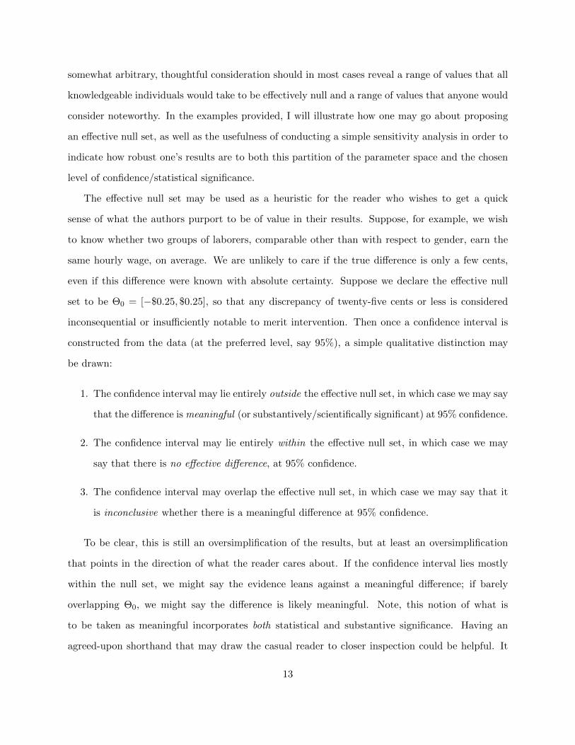
even if this di↵erence were known with absolute certainty. Suppose we declare the e↵ective null

set to be ⇥0 = [�$0.25, $0.25], so that any discrepancy of twenty-five cents or less is considered

inconsequential or insu�ciently notable to merit intervention. Then once a confidence interval is

constructed from the data (at the preferred level, say 95%), a simple qualitative distinction may

be drawn:

1. The confidence interval may lie entirely outside the e↵ective null set, in which case we may say

that the di↵erence ismeaningful (or substantively/scientifically significant) at 95% confidence.

2. The confidence interval may lie entirely within the e↵ective null set, in which case we may

say that there is no e↵ective di↵erence, at 95% confidence.

3. The confidence interval may overlap the e↵ective null set, in which case we may say that it

is inconclusive whether there is a meaningful di↵erence at 95% confidence.

To be clear, this is still an oversimplification of the results, but at least an oversimplification

that points in the direction of what the reader cares about. If the confidence interval lies mostly

within the null set, we might say the evidence leans against a meaningful di↵erence; if barely

overlapping ⇥0, we might say the di↵erence is likely meaningful. Note, this notion of what is

to be taken as meaningful incorporates both statistical and substantive significance. Having an

agreed-upon shorthand that may draw the casual reader to closer inspection could be helpful. It

13

is not the oversimplification represented by p-values and asterisks per se that threatens scientific

understanding, but rather that such features draw focus away from what matters most. In this

a UST presentation, the simplification addresses what is of scientific interest (the magnitude of a

parameter) while simultaneously providing evidence as to whether we can have some confidence

that a seemingly meaningful result is not a phantom.

A unified approach to statistical and practical significance really just constitutes formalized

recognition that without substantive reasoning, signal-to-noise ratios are devoid of meaning. A

key virtue of such a framework is that it forces an explicit declaration of what the scientist would

consider a meaningful, or interesting, result. A good practice is to do the following: Ask yourself,

if you could have perfect and infinitesimally precise knowledge of a parameter’s value, with zero

sampling error, would you know whether you should be impressed with this value? If not, then

any inference from a sample is a waste of time. Thus, when employing a testing paradigm, the

declaration of thresholds of real-world significance is a necessity.

Two other troubling aspects of NHST are addressed by a unified significance testing framework

outlined below. First, by never forcing a point null hypothesis to compete with a composite

(interval) research hypothesis, one abandons the aforementioned practice of using H0 as a straw dog

that is known to be false before data are even examined. Instead, it will be at least hypothetically

possible to legitimately find in favor of the null hypothesis. As n gets large, the width of the

resulting confidence interval will shrink until it lies entirely in either the e↵ective null interval or

the alternative. Finally, the awkward and disingenuous embrace of one-sided hypotheses of the form

H0 : ✓ < ✓0 vs. H1 : ✓ = ✓0 is banished as counterintuitive and unjustified. The use of one-tailed

tests has itself long been the subject of controversy (see, e.g., Eysenck (1960)), in part because of

the nagging suspicion that that they are employed more out of a desire to compensate for poor

power to reject the null than for theoretically driven reasons. They would be replaced by one-sided

hypotheses that are genuinely commensurable: H0 : ✓ < ✓0 vs. H1 : ✓ � ✓0.

In Figure 1, I plot confidence intervals for hypothetical results one might obtain in addressing

the wage di↵erence question. Since the results are imagined, let’s suppose for the sake of concrete-

ness, that they are 95% confidence intervals (one could also superimpose two or three confidence

14

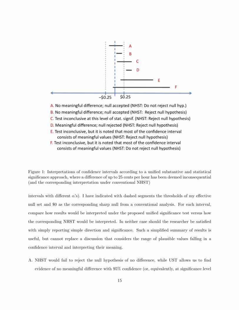
Figure 1: Interpretations of confidence intervals according to a unified substantive and statisticalsignificance approach, where a di↵erence of up to 25 cents per hour has been deemed inconsequential(and the corresponding interpretation under conventional NHST)

intervals with di↵erent ↵’s). I have indicated with dashed segments the thresholds of my e↵ective

null set and $0 as the corresponding sharp null from a conventional analysis. For each interval,

compare how results would be interpreted under the proposed unified significance test versus how

the corresponding NHST would be interpreted. In neither case should the researcher be satisfied

with simply reporting simple direction and significance. Such a simplified summary of results is

useful, but cannot replace a discussion that considers the range of plausible values falling in a

confidence interval and interpreting their meaning.

A. NHST would fail to reject the null hypothesis of no di↵erence, while UST allows us to find

evidence of no meaningful di↵erence with 95% confidence (or, equivalently, at significance level

15

.05).

B. Under NHST, one would reject H0 and find a di↵erence in wages to be statistically significant;

under UST, the finding still favors no meaningful di↵erence in wages, at ↵ = .05.

C. Under NHST, one would again reject H0 at ↵ = .05, while the corresponding unified test

would be inconclusive (though the researcher would indicate that all values in the interval were

positive, including both notable values and ones only trivially positive).

D. The NHST and UST both find a significant di↵erence; in the case of the former, the di↵erence

may only be called statistically significant, while by the latter, one may say that a meaningful

di↵erence is detectable.

E. While the null hypothesis is rejected under NHST (a sensible outcome), UST finds inconclusive

results. Sensitivity analysis would confirm what is evident in the picture—a slight change in

either ↵ or the defined ⇥0 would allow rejection of the null both on statistical and substantive

grounds. Furthermore, the wide confidence interval includes only a sliver of the e↵ective null set,

but a wide range of consequential values, meaning a nuanced consideration of the results should

grant the researcher some legitimacy in claiming evidence of a meaningful wage di↵erence and

calling for a study with a greater number of observations to gain precision.

F. Note that NHST, while rejecting the null for interval E., would not reject it for F. UST would

again claim inconclusive results, defensible due to the lack of precision.

Stated precisely, in algorithmic form, a unified significance test includes the following steps, assum-

ing a continuous parameter space:

Unified Substantive and Statistical Significance Test (UST)

I Partition the parameter space ⇥ for each estimate of interest into ⇥0, an e↵ective null set and⇥1, a set of meaningful values, both non-countable sets corresponding to composite hypotheses.

II Defend the choices of each partition either through topic-specific theory or everyday explana-tion.

III Estimate parameters using confidence intervals.

16

IV For an estimated 1� ↵ confidence interval C,

(a) Find in favor of the null hypothesis of no meaningful “e↵ect” if C ⇢ ⇥0, with 1 � ↵confidence,

(b) find in favor of the alternative hypothesis of a meaningful “e↵ect” if C ⇢ ⇥1, with with1� ↵ confidence,

(c) or declare the result inconclusive at 1 � ↵ if C \ ⇥0 6= ; and C \ ⇥1 6= ;, i.e., if theconfidence interval overlaps the two sets of values.

V Employ sensitivity analysis to determine whether other reasonable partitions of ⇥ or choicesof ↵ would have a↵ected the outcome of the test.

VI Discuss and interpret the confidence intervals in context, noting the range of likely e↵ect sizes.In particular, if the result must be declared inconclusive at the selected ↵, the analyst should,for example, distinguish between a fairly precise confidence interval containing parameter val-ues either in or close to the e↵ective null set and one that is wide (less precise), but containingmostly values considered to be substantively significant and perhaps even large.

4 Two Illustrations of Unified Significance Testing

A major problem involved in adjudicating the scientific significance of di↵erences isthat we often deal with units of measurement we do not know how to interpret (Carver,1978).

I shall next illustrate how unified significance testing may enrich the presentation and interpre-

tation of results. In certain instances, the UST framework for considering results may strengthen

authors’ arguments; in other cases it makes more obvious the tentativeness with the results should

be viewed. Most importantly, however, a unified approach to significance shifts the emphasis to

practical significance, giving it the focus deserved.

4.1 Media E↵ects on Public Opinion: Support for Military vs. Diplomatic

Response as Function of Exposure to Television News

Within their article exploring the three most widely studied types of media e↵ects (agenda-

setting, priming, and framing) in the context of the lead up to the Persian Gulf War of 1990-91,

Iyengar and Simon (1993) consider whether exposure to television news may predict support for

a military response to Iraq’s invasion of Kuwait and the subsequent crisis. Having studied eight

17

months of prime-time newscasts during the relevant time interval, they note the predominant use

of episodic over thematic framing; based on extant theory and previous research, they suspect that

this will lead to viewers’ attribution of responsibility to particular individuals and groups rather

than broader historical, societal or structural causes, and anticipate that this will translate into

support for the use of military force against Saddam Hussein rather than diplomatic strategies

by those who consume such media. They regress a variable measuring respondent support for a

military over diplomatic response on several predictors, via OLS.

According to the logic of a unified significance testing approach, it is essential that one con-

sider what magnitudes of coe�cients would be impressive if one were able to observe the parameter

values themselves without sampling error. Iyengar and Simon are primarily concerned with the

expected e↵ect on military support corresponding to variation in the values of TV News Exposure

and Information, measures of, respectively, television news consumption and awareness of political

information via identification of political figures in the news. Controlling for party, gender, race,

education and general support of defense spending, what sort of coe�cients should we view as e↵ec-

tively zero and, conversely, what values would indicate at least a somewhat meaningful relationship?

This sort of question, as noted before, is too often left unasked. To the extent that it does arise,

it is almost always handled completely informally. To their credit, the authors here distinguish

between the two types of significance: “Overall, then, there were statistically significant traces of

the expected relationship. Exposure to episodic news programming strengthened, albeit modestly,

support for a military resolution of the crisis.” From a unified significance testing—rather than

NHST—perspective, the assessment of the degree to which this type of programming corresponds

to greater military support is of principal concern.

The Iyengar-Simon model may be written as :

MilitarySupport = �0 + �1TV news+ �2Info+ �3(Male⇥Info) + �4(nonWhite⇥Info)

+ �5Male+ �6nonWhite+ �7Republican+ �8DefenseSpend+ �9Educ+ ✏

(1)

18

The predictors of primary interest are TV news, the number of self-reported days per week watching

TV news, and Information (or Info), the respondent’s score from 0 to 7 on a quiz of recognition

of political figures, taken as another proxy for news consumption. In Iyengar and Simon’s model,

the contribution of Info (but not TV news) is allowed to vary by race and gender (through the

inclusion of interaction e↵ects), so that one might wish to discover whether the following parameters

are of a meaningful magnitude:

�1 = �2 = e↵ect of Info among White Females

�2 = �2 + �3 = e↵ect of Info among White Males

�3 = �2 + �4 = e↵ect of Info among non-White Females

�4 = �2 + �3 + �4 = e↵ect of Info among non-White Males

(2)

For each demographic category, the associated coe�cient is interpreted as the di↵erence in

expected level of support for a military solution associated with an additional point on the political

knowledge quiz. Thus, for example, if �1 = 0.25, this means that one might expect an extra correct

answer on the quiz taken by a White Female to correspond to an additional quarter-point on the

scale from 0 to 4, assuming that the ordinal scale of support for diplomacy vs. military action can

be sensibly interpreted as if it were an interval-level measurement. A large di↵erence of four points

on the quiz (e.g., correctly identifying six rather than two political figures, or four rather than zero),

would be expected to translate into a full unit increase in the support for a militaristic solution on

the scale of 0 to 4.2 Understanding this allows the researcher to set up reasonable expectations of

what might be considered a truly meaningful “e↵ect” and then evaluate whether the data support

such a finding in light of sampling error.

Following the steps outlined above, one would begin by declaring a reasonable null set. Three

2Specifically, one point was awarded if the respondent supported tougher military action going forward, ratherthan any of three less hawkish alternatives, and up to three points were awarded for level of militarism expressedin response to the question of what the United States should have done as an original response to the Persian Gulfcrisis.

19

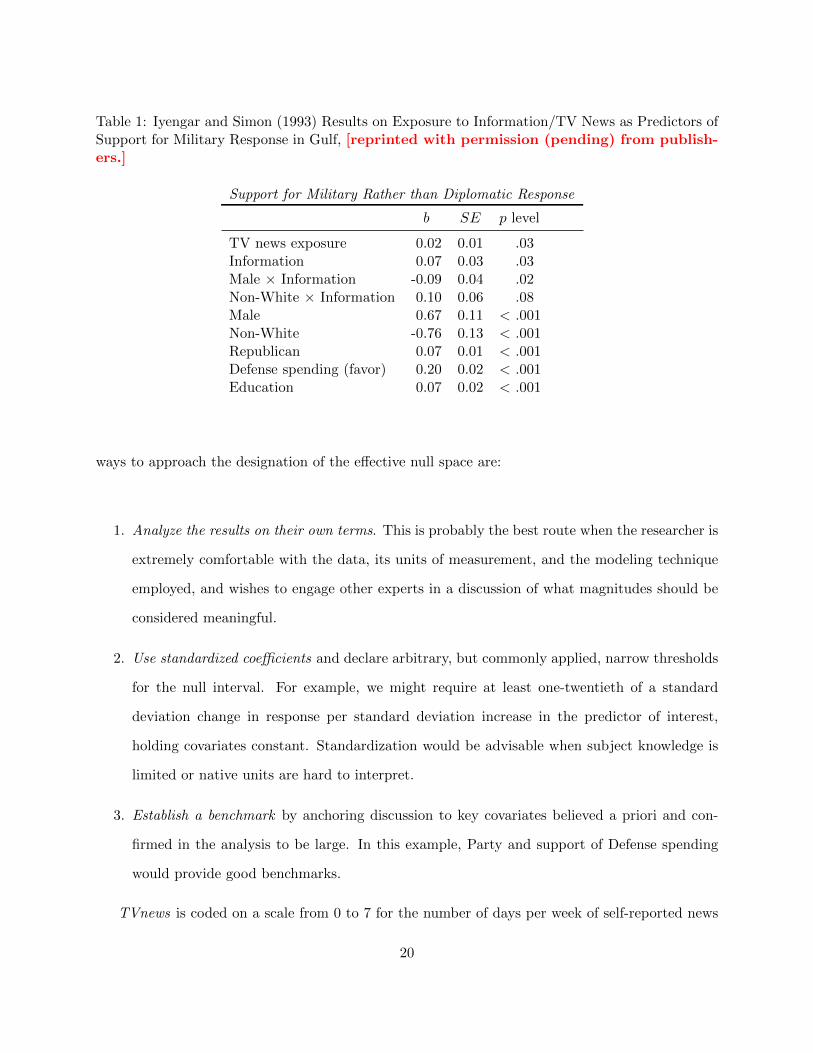
Table 1: Iyengar and Simon (1993) Results on Exposure to Information/TV News as Predictors ofSupport for Military Response in Gulf, [reprinted with permission (pending) from publish-ers.]

Support for Military Rather than Diplomatic Response

b SE p level

TV news exposure 0.02 0.01 .03Information 0.07 0.03 .03Male ⇥ Information -0.09 0.04 .02Non-White ⇥ Information 0.10 0.06 .08Male 0.67 0.11 < .001Non-White -0.76 0.13 < .001Republican 0.07 0.01 < .001Defense spending (favor) 0.20 0.02 < .001Education 0.07 0.02 < .001

ways to approach the designation of the e↵ective null space are:

1. Analyze the results on their own terms. This is probably the best route when the researcher is

extremely comfortable with the data, its units of measurement, and the modeling technique

employed, and wishes to engage other experts in a discussion of what magnitudes should be

considered meaningful.

2. Use standardized coe�cients and declare arbitrary, but commonly applied, narrow thresholds

for the null interval. For example, we might require at least one-twentieth of a standard

deviation change in response per standard deviation increase in the predictor of interest,

holding covariates constant. Standardization would be advisable when subject knowledge is

limited or native units are hard to interpret.

3. Establish a benchmark by anchoring discussion to key covariates believed a priori and con-

firmed in the analysis to be large. In this example, Party and support of Defense spending

would provide good benchmarks.

TVnews is coded on a scale from 0 to 7 for the number of days per week of self-reported news

20

watching, and Info is measured as an additive score of correct answers on a political identification

quiz, again from 0 to 7. The dependent variable ranges in value from 0 (the most diplomatic) to

4 (the most militaristic). Thus, the coe�cient on TVnews is meant to be the expected change in

military support corresponding to an extra day per week watching the news.

The table of results provided in the original article, shown here in Table 1, is not especially

informative. The authors discuss the results in vague terms, and the manner in which these

inferences are being drawn is unclear:

Partisanship, race, gender, and education—all a↵ected respondents’ policy prefer-ences concerning resolution of the conflict. Republicans, males, those with more educa-tion, and Whites tended to support the military option. Support for increased defensespending was strongly associated with a more militaristic outlook toward the conflict.Both indicators of exposure to television news exerted significant e↵ects—more informedrespondents and respondents who watched the news more frequently were most apt tofavor a military resolution. The e↵ects of information were markedly stronger amongwomen and minorities. . . (Iyengar and Simon (1993), my emphasis)

As is the norm, the assessments here are all-or-nothing. Predictors either “a↵ected” outcomes

or not, and the meaning of “significant e↵ects” is left unspoken, as is the origin of the judgment

that e↵ects were “markedly stronger” among certain groups. Indeed, not having to think about or

communicate what meaningful results would look like makes it easier to get away with not actually

interpreting the interaction e↵ects.

Using the benchmark approach discussed above, consider a possible UST analysis based on the

reported point estimates and hypothetical estimated variances.3 The 95% confidence interval for

support of defense spending is (0.16, 0.24), but for simplicity, consider the point estimate, 0.20.

The variable measures response to whether the nation should decrease or increase defense spending

on a scale from greatly decrease (1) to greatly increase (7). Informally, looking at the predicted

e↵ect of a one-level jump in support for defense spending (a unit increase if this were treated as an

intervel-level, rather than ordinal measurement), or a moderate (say 2 levels) or large (say 4 levels,

e.g. from 2 to 6) shift, provides a decent benchmark for comparison. One wouldn’t expect that

3We would need the estimated covariances among coe�cients to obtain approximate standard errors for the

estimates of each � since, for example, s.e. (�̂2) =

rVar

⇣�̂2

⌘+Var

⇣�̂3

⌘+ 2Cov

⇣�̂2, �̂3

⌘. For the hypothetical

values, actual estimated variances are taken from the original paper and the covariance terms are set to zero).

21

a more subtle predictor such as TV watching would possibly match the predictive power of the

respondent’s general pre-disposition towards a muscular defense, but it would be tough to argue

that a magnitude absolutely dwarfed by this benchmark variable would still be noteworthy. These

are measured in di↵erent units, so it would be preferable to compare standardized versions, but

the units are interpretable enough to be analyzed intuitively. With the expectation that support

for defense should be a major driver of the response variable, what might we establish as a bare

minimum for the e↵ect of an extra day of watching TV news? More specifically, since a large

di↵erence in general militarism (say between 1 and 6 or between 2 and 7) is expected to correspond

to a unit di↵erence on specific militarism in the Gulf (between 1 and 2, or 2 and 3 on the four-point

scale, for example), how much of a change should accompany a large di↵erence in TV-news-watching

(say one vs. six days per week) in order for us to be mildly impressed? Let us require at least one-

tenth of a unit on this scale, which would represent somewhat of a blip compared to the observed

e↵ect of Defense. This translates to a coe�cient value of at least 0.02 (since 5⇥0.02 = 0.10). Thus,

an e↵ective null set of (�0.02, 0.02), for example, on either of the key predictors (both of which

are scaled from 1 to 7, just as the defense question) would be generous. Somewhere upwards of

.05 in either direction might be taken as substantial, and beyond the benchmark of .20 would be

stunningly large.

Consider what is communicated by a UST results summary, a portion of which appears in Table

2, as opposed to the NHST-based original Table 1. Aside from Defense Spending, the baseline used

to anchor our judgment of e↵ect size, where can we distinguish meaningful associations? The

authors assert a “markedly stronger” e↵ect of information on minorities and women, but is this

so? Looking at the UST results, no such relationship is detected for non-white men. Information

makes a meaningful di↵erence specifically for some women, it would seem. For non-white women,

in particular, greater information exposure clearly corresponds to higher expected level of support

for military intervention, all else equal. For white women, the relationship likely exists as well; the

point estimate is 0.06 and the 95% confidence interval barely overlaps the chosen null interval, and

does not at all at 80% confidence. In both cases, the association may actually be quite large; a

sample with more women would increase the estimate precision. Controlling for level of information

22

Table 2: Hypothetical Results for Unified Significance Test of Exposure to Information/TV Newsas Predictors of Support for Military Response in Gulf

Support for Military Rather than Diplomatic Response

E↵ective null 95% CI Hypothetical Finding

TVnews �1 [-0.02,0.02] [0.00,0.04] Indistinguishable from null set4

Info (White Females) �1 [-0.02,0.02] [0.01,0.13] H0 would be rejected at 80% conf.Info (White Males) �2 [-0.02,0.02] [-0.12,0.08] Indistinguishable from null setInfo (Non-White Females) �3 [-0.02,0.02] [0.03,0.31] H0 rejected/ H1 supportedInfo (Non-White Males) �4 [-0.02,0.02] [-0.18,0.34] Indistinguishable from null setDefenseSpend �8 [�1,0.10] [0.16,0.24] H0 rejected/H1 supported

detected by Info, as well as the other variables, exposure to television news is not predictive of the

dependent variable at a level distinguishable from the null set. If an e↵ect is there, it is likely

relatively small in magnitude. If the coe�cient on TV news exposure is .05, just on the upper

margin, this would mean someone who watches much more news would, all else equal, would get an

expected boost of just one-fifth of a unit (measured from 0 to 4) in support for military intervention.

None of this nuance is available in the original table.

In basic regressions or di↵erence-in-mean tests, consideration of scientific significance is often

overlooked. When modeling choices make substantive interpretation more di�cult, it becomes ever

more tempting to rely purely on p-values produced in standard output as the primary evidence.

We have just seen an example of this, where interaction e↵ects are present. Next we turn to an

example in which a transformation of variables complicates matters somewhat.

4.2 Transformation of Variables: An Example from Voting Behavior

Even the best research can be led astray by prioritizing statistical significance over substantive

interpretation. Consider the excellent contribution by Gasper and Reeves (2011), who examine

evidence for a number of hypotheses about how voters might reward or punish incumbent politicians

for their responses to damaging events beyond their control. The authors posit an “attentive

4The hypothetical confidence interval overlaps the null set and the meaningful positive values; the estimate isthus statistically indistinguishable from a negligible result, but a positive and meaningful relationship would not beinconsistent with the estimate and uncertainty.

23

electorate,” who should be expected to reward governors requesting disaster aid and presidents

who grant it, and punish those who do not.

Overall, the study is thorough and convincing, with respect to the conjectures about how gov-

ernors and presidents may be punished for their actions, in large part because the authors go

beyond simply reporting signs of coe�cients and statistical significance, and attempt to translate

their models’ predictions in context (e.g., a successful request for disaster aid is associated with an

average additional 2% vote for incumbent governors, controlling for included covariates.) However,

one of the more surprising conclusions in the study, that voters punish incumbent governors and

presidents in part based purely upon the extent of local weather damage itself, is revealed under

UST to lack practical significance.5 The authors make the following claims:

Governors. “The e↵ects of weather damage are not insubstantial. If a weather event causes

approximately $1,950 worth of damage per 10,000 citizens, it will cost the incumbent governor 1

point at the ballot box.”

Presidents. “Like the results for gubernatorial elections . . . , presidents are punished for se-

vere weather damage. For example, $20,000 in weather damage in a county of 10,000 voters would

result in a modest decrease of a quarter point in the two-party popular vote.”

The authors’ emphasis on meaningful interpretation of magnitudes is commendable, but the

UST requirement that one declare an e↵ective null set, demands a level of scrutiny that would

have led to a di↵erent conclusion. In Figure 2, I have appended a few of the dollar amounts (per

10,000 citizens) corresponding to log-dollars in the original histogram. The impact of an additional

$1000 or so means an increase of 2 in log-dollars if the change is from 5 to 7 ($148 to $1167); this

corresponds to an expected drop in support for incumbent governors of �.13(2), just a quarter

of a percent. This same di↵erence in support is predicted by this model in comparing a county

5One should be especially hesitant to make too much of statistical significance when the number of observations arelarge. Confronted with n’s of around 15,000 or 25,000, as in Gasper and Reeves (2011), uncertainty due to samplingerror becomes negligible, with the impact of any such sampling variation likely dwarfed by the measurement error ormisspecification error in the model.

24

Figure 2: Logged Damage and Corresponding Amounts in Dollars, based on Gasper and Reeves(2011, pending approval)

su↵ering 3.27 million dollars of damage per ten-thousand citizens and one with 8.89 million dollars

(from 15 to 17 on the log-scale). In using a logarithmic transformation on cost of weather damage,

the authors implicitly accept a nonlinear impact on voting, not an unreasonable assumption. The

consequence, however, is that they need to think in terms of exponential increases in damage

in order to decide whether the explanatory power of weather damage is notable. Rather than

evaluating the impact of $1950 in damage (not interpretable in absolute terms on a logarithmic

scale), the relevant question is: What would be a meaningful penalty, in % of vote share, based on

percentage increase in damage from weather?

In testing the responsive electorate hypothesis, a unit change in the weather damage variable

is in fact a unit change in the natural log of dollars of damage per ten thousand people. If one is

25

Significance Level

Thre

shol

d fo

r Mea

ning

ful E

ffect

0.01 0.05 0.09 0.13 0.17

0.05

0.20

0.35

0.50

0.65

0.80

(a) Governor

Significance Level

Thre

shol

d fo

r Mea

ning

ful E

ffect

0.01 0.05 0.09 0.13 0.17

0.05

0.20

0.35

0.50

0.65

0.80

(b) President

Significance Level

Thre

shol

d fo

r Mea

ning

ful E

ffect

0.01 0.05 0.09 0.13 0.17

0.05

0.20

0.35

0.50

0.65

0.80

(c) Rain

Figure 3: Who’s to Blame for Weather Damage? Findings in favor of (light) or against (dark)a statistically and substantively significant relationship between weather damage and change insupport for incumbent governor, incumbent president, or (fabricated) rain. Inconclusive resultsappear in light gray.

to interpret this directly in more meaningful way, it is important to remember that the log-units

represent a multiplicative scale; specifically, each unit increase in X means nearly a tripling of per

capita damages.6 What is the minimal change one would need to see in the dependent variable

for a particular increase in the covariate of interest in order to be impressed? For example, say I

declare that I would need to see at least a one-percent drop in vote-share for damage increased by

a factor of around 150 (or, equivalently, an additive log-dollar increase of five). That is, anything

less than a penalty of 1% at the ballot box for $22,000 vs. $150 in damages per 10,000 people, or

$3.27 million vs. $22,000, would be deemed inconsequential.

One way to address the sensitivity of results to one’s choice of e↵ective null set as well as the

(equally arbitrary) choice of statistical significance level is by revealing what pairings (↵, �) would

yield a “decision” in agreement with the one actually made, where ↵ is statistical significance level

and � is the distance on either side of the conventional sharp null parameter deemed e↵ectively

null.7 For example, in the first two frames of Figure 3, I have indicated with a dashed line my

6The base of the log determines the multiplicative constant—here, the authors use the natural log, with a base ofaround 2.718, so, for example, a move from 1 to 2 or 4 to 5 or 8 to 9 on the log scale means multiplying by a factor of2.7. Similarly, a jump of five on the log scale means multiplication by a factor of (2.718)5 or 148 times the lower value.There is nothing gained by using the natural base here; for ease of interpretation, a base-2 or base-10 logarithmictransformation might be be preferable, since these correspond to doubling or multiplying by ten, respectively.

7For simplicity, I suppose the range of null values is symmetric about a point null, but this is not necessary.

26

choice of �, a coe�cient of 0.20 as defended above. Decision values are plotted for values of ↵

from .001 to .200 and for values of � from one-fourth of my chosen value of .20 to four times that

value i.e., in [.05, .80]. In considering whether weather damage alone predicts a (statistically and

substantively) significant di↵erence in average support for an incumbent governor, controlling for

various covariates including response by governor and president, my answer of No is not sensitive

to choice of ↵, but is somewhat sensitive to my threshold of substantive significance. If my e↵ective

null set had been slightly smaller, I would have found the results inconclusive at ↵ = .05. On the

other hand, all reasonable values of (↵, �) lead to the same conclusion: No significant relationship.

Finally, just to have a look at other possible output one might have to interpret, imagine a

hypothetical public opinion survey asking citizens in each county whether they like rain, then mod-

eling percentage pro- and anti-rain according to the same covariates as before. Here, at significance

levels of .05 or .10, we would find a significant relationship between logged-dollars of damage per

ten thousand citizens and sentiment toward rain, but at ↵ below 0.01, we would have (just barely)

found the results inconclusive. Similarly, a wider e↵ective null set (e.g., if a regression coe�cient

of less than 0.50 were deemed uninteresting, meaning a 7.4-fold increase in damage (plus 2 in log-

dollars) would need to be accompanied by no less than a one-percent drop in support for Rain to

be worthy of note) would make us hesitant to reject the null hypothesis.

5 Conclusions

The criticisms of null hypothesis significance testing as commonly put into practice are widely

recognized and not especially controversial among statisticians. Despite having been aired in nu-

merous forums over the decades—at least outside of political science—not much has changed in

terms of standard practice. Bayesian approaches to hypothesis testing, focusing attention directly

on the relative probabilities of competing hypotheses in light of data, do not su↵er the principal

failings of the NHST, and so the growing acceptance of the Bayesian toolkit has been a source

of improvement on this front. Within a frequentist framework, however, debates over the merits

of significance testing have had little impact on practice. It is di�cult to change habits while

the status quo is rewarded and no consensus, nor even clear guidance on a preferable alternative

27

emerges. Within non-Bayesian analysis, I recommend that a unified (scientific and statistical)

significance testing approach be adopted as standard practice in summarizing the results of quan-

titative empirical analyses. The expectation that scholars consider magnitudes of parameters of

interest, and not simply distinguish signal from noise, requires little additional work and no special

training, but guides us in the direction of meaningful discussion and away from the seductive lure of

empty formalism. Additionally, to convincingly argue about what results should be deemed signif-

icant in practical terms provides incentive for creative intertwining of qualitative with quantitative

knowledge of subject matter.

In fact, the simple approach that I have called UST (to contrast it with NHST) is simply a

formalization of certain principles of sound statistical reasoning, which are no doubt second-nature

to many seasoned scientific professionals. If formally stated results of hypotheses tests continue to

be the norm in scientific journals, it would restore some amount of balance to insist that scientific

or practical significance be given at least equal attention in summaries of results such as those

typically provided in tables and figures. Here I have outlined the bare essentials of what a unified

approach should look like. Since presenting early versions of this work, I have encountered two sets

of writings that address related themes within biostatistics and medical diagnostics literatures; these

literatures, largely unknown among social scientists, o↵er a more extensive framework for just this

sort of balanced approach. Two excellent books outline the process of generating and evaluating

“informative hypotheses” (Hoijtink, 2011; Hoijtink et al., 2008) within a Bayesian perspective.

Also especially relevant is work on minimal clinically important di↵erence (MCID). Key articles

include Jaeschke, Singer and Guyatt (1989); ?); Copay et al. (2007). The consequences of mistaking

statistical significance for practical significance surely have higher stakes in such matters as pain

reduction or medical risk assessment, so it is surprising not to see such areas begin to embrace this

sort of approach before social science, but only that it has taken so long.

References

Altman, M., ed. 2004. “Introduction to special issue on statistical significance.” Journal of Socio-

Economics 33(5):523–675.

28

Arbuthnot, J. 1710. “An argument for Divine Providence, taken from the constant regularity

observed in the births of both sexesrovidence, taken from the constant regularity observed in the

births of both sexes.” Philosophical Transactions of the Royal Society 27:186–190.

Boring, E.G. 1919. “Mathematical vs. scientific significance.” Psychological Bulletin 16(10):335.

Carver, R.P. 1978. “The case against statistical significance testing.” Harvard Educational Review

48(3):378–399.

Cohen, J. 1994. “The world is round (p¡. 05).” American Psychologist 49:997–1003.

Copay, Anne G, Brian R Subach, Steven D Glassman, David W Polly Jr and Thomas C Schuler.

2007. “Understanding the minimum clinically important di↵erence: a review of concepts and

methods.” The Spine Journal 7(5):541–546.

DeGroot, M.H. and M.J. Schervish. 2002. Probability and statistics. Boston: Addison-Wesley.

Esarey, J. 2010. “A Formal Test for Substantive Significance.” Available on-line. URL:

http://userwww. service. emory. edu/˜ jesarey/riskstats. pdf .

Eysenck, HJ. 1960. “The concept of statistical significance and the controversy about one-tailed

tests.” Psychological Review 67(4):269–271.

Falk, Ruma and Charles W Greenbaum. 1995. “Significance Tests Die Hard The Amazing Persis-

tence of a Probabilistic Misconception.” Theory & Psychology 5(1):75–98.

Finney, David J. 1995. “Frank Yates. 12 May 1902-17 June 1994.” Biographical Memoirs of Fellows

of the Royal Society 41:555–573.

Gasper, J.T. and A. Reeves. 2011. “Make it Rain? Retrospection and the Attentive Electorate in

the Context of Natural Disasters.” American Journal of Political Science .

Gelman, A. and H. Stern. 2006. “The di↵erence between “significant” and “not significant” is not

itself statistically significant.” The American Statistician 60(4):328–331.

29

Gigerenzer, G., Z. Swijtink and L. Daston. 1990. The empire of chance: How probability changed

science and everyday life. Vol. 12 Cambridge Univ Pr.

Gill, J. 1999. “The insignificance of null hypothesis significance testing.” Political Research Quar-

terly 52(3):647.

Harlow, L.L., S.A. Mulaik and J.H. Steiger. 1997. What if there were no significance tests? Lawrence

Erlbaum.

Hodges, JL and EL Lehmann. 1954. “Testing the approximate validity of statistical hypotheses.”

Journal of the Royal Statistical Society. Series B (Methodological) 16(2):261–268.

Hoijtink, H. 2011. Informative Hypotheses: Theory and Practice for Behavioral and Social Scien-

tists. Chapman & Hall.

Hoijtink, H., I. Klugkist, P.A. Boelen and SpringerLink (Service en ligne). 2008. Bayesian evaluation

of informative hypotheses. Springer.

Iyengar, S. and A. Simon. 1993. “News coverage of the Gulf crisis and public opinion.” Communi-

cation Research 20(3):365–383.

Jaeschke, R., J. Singer and G.H. Guyatt. 1989. “Measurement of health status:: Ascertaining the

minimal clinically important di↵erence.” Controlled clinical trials 10(4):407–415.

Je↵reys, S.H. 1961. Theory of probability. Clarendon Press.

Kish, L. 1959. “Some statistical problems in research design.” American Sociological Review

pp. 328–338.

Levin, J.R. 1998. “What if there were no more bickering about statistical significance tests.”

Research in the Schools 5(2):43–53.

Meehl, P.E. 1978. “Theoretical risks and tabular asterisks: Sir Karl, Sir Ronald, and the slow

progress of soft psychology.” Journal of consulting and clinical Psychology 46(4):806.

30

Morrison, D.E. and R.E. Henkel, eds. 1970. The Significance Test Controversy: A Reader. Chicago:

Aldine.

Rosenthal, R. 1979. “The” File Drawer Problem” and Tolerance for Null Results.” Psychological

Bulletin 86(3):638–641.

Schrodt, P.A. 2006. “Beyond the Linear Frequentist Orthodoxy.” Political Analysis 14(3):335–339.

Tukey, John W. 1991. “The philosophy of multiple comparisons.” Statistical Science pp. 100–116.

Tyler, R.W. 1931. “What is statistical significance?” Educational Research Bulletin pp. 115–142.

Verzani, J. 2005. Using R for introductory statistics. CRC Press.

Ward, M.D., B.D. Greenhill and K.M. Bakke. 2010. “The perils of policy by p-value: Predicting

civil conflicts.” Journal of Peace Research 47(4):363–375.

Yates, F. 1951. “The influence of statistical methods for research workers on the development of

the science of statistics.” Journal of the American Statistical Association 46(253):19–34.

Yule, G.U. 1919. An introduction to the theory of statistics. C. Gri�n and company, limited.

Ziliak, S.T. and D.N. McCloskey. 2008. The cult of statistical significance: How the standard error

costs us jobs, justice, and lives. Univ of Michigan Pr.

31