Simultaneous Multilateral Search∗

Sergei Glebkin

INSEAD

Bart Zhou Yueshen

INSEAD

Ji Shen

Peking University

January 10, 2022

Abstract

This paper studies simultaneous multilateral search (SMS) in over-the-counter markets:

When searching, a customer simultaneously contacts several dealers and trades with the one

offering the best quote. Higher search intensity (how often one can search) improves welfare,

but higher search capacity (how many dealers one can contact) might be harmful. When the

market is in distress, customers might inefficiently favor bilateral bargaining (BB) over SMS.

Such preference for BB speaks to the sluggish adoption of SMS trading, like request-for-quote

protocols, in over-the-counter markets. Furthermore, a market-wide shift to SMS may not be

socially optimal. (JEL D40, D84, G12, G14)

∗We are grateful to Itay Goldstein (the editor) and two anonymous referees for their tremendous help throughoutthe review process. We also benefit immensely from discussions with Markus Baldauf, Jean-Edouard Colliard, PierreCollin-Dufresne, Jerome Dugast, Maureen O’Hara, Uday Rajan, Ioanid Rosu, Gideon Saar, Dimitri Vayanos, KumarVenkataraman, Sebastian Vogel, Zhuo Zhong, Haoxiang Zhu, and Junyuan Zou. In addition, comments and feedbackare greatly appreciated from participants at conferences and seminars at Cornell, EFA 2020, Collegio Carlo Alberto,EPFL, LSE, and INSEAD. Send correspondence to Bart Zhou Yueshen, b@yueshen.me.

Search is a key feature in over-the-counter (OTC) markets. Duffie, Garleanu, and Pedersen

(2005, hereafter DGP) pioneered the theoretical study of OTC markets in a framework of ran-

dom matching and bilateral bargaining (BB): Investors search for counterparties and are randomly

matched over time. Upon successful matching, a buyer and a seller engage in Nash bargaining and

split the trading gain according to their endowed bargaining power.

However, investors’ interaction is not always bilateral. For example, in recent years, there is a

rise of electronic trading in OTC markets, mainly in the form of Request-for-Quote (RFQ). In such

marketplaces, where many corporate bonds and derivatives are traded, a customer contacts multiple

dealers for quotes and then trades with the one offering the best price. Hendershott and Madhavan

(2015) report that more than 10% of trades in the $8tn corporate bond market is completed via

RFQ. O’Hara and Zhou (2021) document a continued growth of RFQ-based trading of corporate

bonds, but only sluggishly, with the highest trading volume share below 14% in their sample.

This paper develops a theoretical model, tailored to the above one-to-many searching. Specif-

ically, a customer is allowed to query multiple dealers at the same time, hence the name “Simul-

taneous Multilateral Search” (SMS). The objective is twofold. First, we examine how the SMS

technology affects assets allocation and welfare. Second, we study how customers choose to search:

Do they favor SMS over BB? Are their choices efficient? How do we understand the sluggish growth

of SMS-type of electronic trading (O’Hara and Zhou, 2021)?

Section 1 sets up the model following Hugonnier, Lester, and Weill (2020, hereafter HLW), where

a continuum of customers trade an asset through a continuum of homogeneous dealers.1 All agents

can hold either zero or one unit of the asset. The customers are subject to stochastic valuation

shocks. Those who hold the asset but have low valuation want to sell, while those without the asset

but with high valuation want to buy. They actively search for dealers according to independent

Poisson processes with intensity ρ. We generalize the search process as follows to model SMS: (i)

each searching customer can request quotes from up to n dealers; (ii) the best quote is determined

via a first-price auction and (iii) the customer can potentially improve upon the best quote via

bargaining: with probability q, the customer can make a take-it-or-leave-it offer (TIOLIO) to the

1 In HLW the dealers are heterogeneous. We abstract from dealer heterogeneity to focus on SMS in a parsimoniousway.

1

winning dealer after the auction. Notably, the search process nests BB as a special case when n = 1:

The searching customer randomly contacts one dealer and sets the price with probability q. With

probability 1− q, the dealer sets the price. In that special case the parameter q thus serves as the

customer’s Nash bargaining power parameter, as in DGP and HLW.

Section 2 characterizes the equilibrium and discusses novel findings. Notably, the two search

parameters, the intensity ρ (how frequently one can search) and the capacity n (how many potential

dealers one can reach), have contrasting implications for various equilibrium objects. For instance,

a higher ρ always reduces the sizes of both the buyer- and the seller-customers, improving the asset

allocation and also welfare. In contrast, a larger n can drive up the size of the short-side customers

and possibly hurt welfare.

The key mechanism is a “dealer bottleneck,” arising from the asymmetric effects of n on the

matching of the two sides of the market. To see this, suppose the asset is in excess supply and

90% of the dealers have inventory while the other 10% do not. Let us examine what happens

when the capacity increases from n = 2 to n = 3: For a customer-seller, the matching rate with

a no-inventory dealer increases from 1 − 0.92 = 19% to 1 − 0.93 = 27.1%. Such an improvement

in matching significantly adds to the asset inflow to dealers from customer-sellers. However, the

outflow rate—the matching between customer-buyers and dealer-sellers—only increases by 0.9%,

from 1 − 0.12 = 99% to 1 − 0.13 = 99.9%. The negligible increase of the outflow rate is not at

all enough to balance the significant rise in the inflow rate. That is, the asset is “clogged” at the

dealers, creating a bottleneck that leaves more customer-buyers unmatched.2 This leads to a surge

in unrealized trading gains and may reduce welfare. To emphasize, this bottleneck effect is unique

to the search capacity n. In contrast, the search intensity ρ does not create asymmetry in matching

and always improves welfare.

Such bottlenecks arise in our most general setup. In a specialized application, we allow cus-

tomers to direct their searches to subsets of dealers of their choosing, based on noisy signals of

dealer types. For example, a customer-buyer might have a rough idea of which dealers have in-

2 It is the increase of the unmatched customer-buyers that eventually balances the asset inflow to and the outflowfrom dealers in the steady state equilibrium. Whereas the inflow increases with n via the higher matching rate, theoutflow increases via the increment in the larger customer-buyer population size.

2

ventory, based on recently reported trades. She then optimally directs her searches only to those

dealers for higher matching probabilities. A key parameter is the signal quality ψ, which can be

interpreted as the transparency of dealer inventories. We show that a similar bottleneck can arise

when ψ increases: As customers direct their searches more accurately, the matching on the short

and on the long side is improved asymmetrically, hindering the efficient passing of the asset through

dealers. Our model thus highlights a potential channel for how better inventory transparency might

hurt welfare.

Another insight from the model is how SMS endogenizes the bargaining powers of customers

and dealers. The key is the dual role of “dealer demographics”—how many dealers have the asset in

their inventories and how many do not: As is standard, dealer demographics affect matching (e.g.,

how likely a customer can find a counterparty to trade). New in this model, dealer demographics

also affect the split of trading gains between customers and dealers. For example, if there are many

dealers with inventories, when contacted by a customer-buyer, they will quote more competitively,

as they know that the customer has also contacted n− 1 other dealers, who very likely might also

have inventories to sell. Such fiercer competition cuts more trading gains to the searching customer

and less to the dealers. Thus, SMS endogenizes the bargaining powers, which are by and large

exogenous in existing search models. Further, in equilibrium, the dealers quote according to a

mixed strategy, creating price dispersion despite dealer homogeneity. Notably, the distribution of

such price dispersion is also endogenously determined via dealer demographics.

Section 3 studies the customers’ choices between BB and SMS. We show that the choice ulti-

mately boils down to the comparison between the two technologies’ expected trading gain intensi-

ties, which are the respective products of (i) the search intensity—how frequent one can search, (ii)

the matching rate—how likely it is to find at least one counterparty, and (iii) the expected trading

gain share above—how much trading gain one can get given a match.

At first glance, one might conclude that SMS has advantages for customers over BB in all three

aspects above: (i) it offers faster connection (via electronic platforms), (ii) it allows customers to

contact multiple dealers, and (iii) it encourages the competition among the contacted dealers, hence

giving larger trading gain shares to customers. The analysis, however, reveals a potential downside,

3

especially when customers have , i.e., when q is low in SMS. In this case, the customer’s expected

trading gain is only determined by the endogenous competition among the contacted dealers. When

such competition is insufficient, the customer expects very little, because any matched counterparty

dealer will charge a monopoly price, knowing that she is likely the only counterparty that the

customer can find (out of the n). In contrast, in BB, a customer always has some chances to secure

some positive trading gains, given a positive q in BB.

It is worth emphasizing that the q in SMS (qSMS) and that in BB (qBB) are exogenous model

parameters. For the customers to favor BB over SMS, the model effectively makes an assumption

that the qSMS is lower than qBB, based on the real-world market structure described here. (A more

general condition is given in Lemma 3.) Together with this, the novel equilibrium force of the n

contacted dealers’ competition (or the lack of it) makes it possible that SMS becomes less attractive

than BB.

Indeed, the customers may favor BB over SMS, especially when the asset is in very imbalanced

demand and supply. Consider the case of excess supply. The large number of customer-sellers flood

the dealer sector with the asset, making most of the dealers full in inventory. Consequently, the

remaining customer-sellers find it very difficult to find dealer-buyers. Even if they do, using SMS,

any matched dealer-buyer will knowingly charge a very low monopoly price. Instead, resorting to

BB, customer-sellers can still negotiate prices with dealers. This prediction echoes the empirical

finding in O’Hara and Zhou (2021) that when corporate bonds are downgraded and under fire sell

(i.e., in excess supply), the electronic trading volume share drops. Such an intrinsic tradeoff between

SMS and BB could have hindered the adoption of electronic OTC trading of corporate bonds. This

mechanism complements the existing explanation for customers’ reluctance of using SMS, which

largely relies on the concern of leaking private information to too many dealers (Hendershott and

Madhavan, 2015). This information leakage argument, however, does not explain the downgrade-

induced reduction of electronic volume shares, as downgrades are public information.

The customers’ endogenous choices between BB and SMS also have welfare and market design

implications. The analysis shows that when the asset trades very fast, i.e., for high search inten-

sity ρ, a social planner strictly prefers SMS over BB, simply because SMS offers better matching,

4

which creates large trading gains. Unlike the planner, who ignores the split of trading gains, the

customers might shy away from SMS because the trading gain split there is inferior compared to

BB. Such inefficiency in technology adoption can be reduced by policies and market designs that

incentivizes customers to use SMS. In the model, this can be achieved by setting a large enough q

in SMS, e.g., by allowing customers to further bargain in RFQ platforms, after running auctions

among dealers.

However, such patches might not always work, depending on the characteristics of the asset

traded. For example, when the asset is intrinsically slow, i.e., for sufficiently low search intensity ρ,

having all investors using SMS is not efficient. The intuition goes back to the bottleneck: In the case

of excess supply, for example, the planner would like customer-sellers to use BB and buyers SMS to

reduce the asset inflow into the dealers, so as to mitigate the bottleneck. Such a distinction between

fast- and slow-moving assets is realistic and important. While corporate bonds on SMS trade in a

few minutes (Hendershott and Madhavan, 2015), auctions of collateralized loan obligations (CLOs)

can take a day or two (Hendershott et al., 2020). Asset-specific design and policies should be

considered, as opposed to market-wide, blanket recommendations.

Contribution and related literature

The paper contributes to four strands of the literature. First, adding to the search models of

OTC markets, this paper introduces the possibility for investors to contact multiple potential

counterparties at the same time. Previous search models largely focus on BB as in DGP, Weill

(2007), Vayanos andWeill (2008), Lagos and Rocheteau (2009), Lagos, Rocheteau, andWeill (2011),

Uslu (2019), and HLW. A noteworthy difference is that in SMS, the split of trading gain between

customers and dealers (their respective bargaining powers) is endogenous of the equilibrium dealer

demographics. This feature distinguishes our model from other works that also have multiple dealers

competing simultaneously for a given transaction. For example, Hendershott et al. (2017) consider

a stylized model of how customers choose to form dealer networks. There, a buyer simultaneously

contacts all dealers in her network, who then compete to find the asset for the customer. Similarly,

in Wang (2017), any agent may query quotes within her network simultaneously. In these models,

5

the split of trading gains between dealers and customers is exogenous. In Zhu (2012) and An (2020),

customers sequentially contact possibly multiple dealers and the resulting endogenous trading gain

splits arise due to other frictions like information asymmetry.

Second, this paper contributes to the theory of electronic OTC markets. Vogel (2019) studies

a hybrid OTC market where investors can trade in both the traditional voice market and the

electronic RFQ platform. Liu, Vogel, and Zhang (2017) compare the the electronic RFQ protocol

in an OTC market with a centralized exchange market. Both papers model the RFQ trading

similarly to the current paper, with the key difference being that their RFQ matching rates are

exogenous, whereas they are endogenous of dealer demographics in this paper. Riggs et al. (2019)

study the RFQ trading in Swap Exchange Facilitites. Their analysis highlights order size as an

important determinant of customers’ choice of trading mechanism. Our analysis complements theirs

and highlights another factor, dealer demographics. In a different line, Saar et al. (2020) compare

dealers’ market making (direct liquidity provision) and matchmaking (searching on the customers’

behalf for counterparties) and study the effects of bank dealers’ balance sheet costs.

Third, there is a growing body of literature comparing centralized versus decentralized trading

(Pagano, 1989; Chowdhry and Nanda, 1991) in various aspects. Babus and Parlatore (2017) study

the endogenous formation of fragmented markets due to investors’ strategic behavior. Glode and

Opp (2019) compare the efficiency of OTC and limit-order markets in a setting where investors

endogenously acquire expertise. Lee and Wang (2019) study uninformed and informed investors’

venue choice through an adverse selection channel. Dugast, Uslu, and Weill (2019) examine banks’

choice among centralized trading, OTC trading, or both, in a setting where the banks differ in

their risky asset endowment and in their capacity of OTC trading. This paper instead compares

the conventional voice trading versus the relatively new electronic trading within the OTC setting.

Finally, this paper contributes to the auctions literature with uncertain number of bidders

(see, e.g., the survey by Klemperer, 1999) and to the literature on pricing with heterogeneously

informed consumers (e.g., Butters, 1977; Varian, 1980; and Burdett and Judd, 1983). Apart from

the above literature on OTC markets, applications of such “random pricing” mechanisms are also

seen recently in exchange trading, as in Jovanovic and Menkveld (2021). The main insight from

6

this paper is that such uncertainty about the number of quoters (bidders) can arise endogenously

from the search process.

1 Model setup

Time is continuous. The model concerns the trading of an asset in fixed supply s.

Customers and dealers. There is a continuum of customers with mass mc and a continuum

of dealers with mass md. Both groups are risk-neutral, discount future utility at the same rate r,

and can each hold either zero or one unit of the asset. An asset owner will be denoted by o and a

non-owner n.

The agents derive flow utility when holding the asset. A customer owner derives y(t) ∈

{yh, yl} (high or low), which evolves stochastically according to a continuous time Markov chain:

P[y(t+ dt) = yh| y(t) = yl ] = λudt and P[y(t+ dt) = yl| y(t) = yh ] = λddt, where λd and λu are

the respective switching intensities. A dealer-owner instead derives constant flow utility yd.

In summary, there are four types of customers, {ho, hn, lo, ln}, and two types of dealers,

{do, dn}. Their population size at any time t are denoted by mσ(t) for σ ∈ {ho, hn, lo, ln, do, dn},

with mho(t) +mhn(t) +mlo(t) +mln(t) = mc and mdo(t) +mdn(t) = md.

Both customers and dealers experience independent exogenous exit shocks: at a Poisson inten-

sity fd (resp., fc) a dealer (resp., a customer) leaves the market and gets zero utility flow going

forward. Immediately after leaving, she is replaced by a trader of the same type, so that the total

population sizes, mc and md, do not change.

Search. The setup above follows HLW (with all dealers having the same preference). Notably,

customers cannot contact each other and have to search for dealers to trade with. We generalize

how customers interact with dealers by introducing a trading technology characterized by {ρ, n, q}.

Using the technology, at a Poisson process with intensity ρ, each customer can contact up to n

dealers.3 Each contact by a customer-buyer (-seller) is a “match” if the contacted dealer is of type-do

3 Customers can choose to contact fewer than n dealers. Since there is no cost of contacting more, in equilibrium,they will always choose to contact n dealers. With contact costs, investors in Riggs et al. (2019) choose an interiornumber of contacts. Such a cost does not bring novel insights in the current model and, hence, is set to zero.

7

(-dn). The probability that any given contact turns into a match is πdo for a buyer (πdn for a seller).

A customer-buyer’s probability of finding at least one matching dealer is then 1− (1− πdo)n; and,

similarly, 1− (1− πdn)n for a customer-seller. Both πdo and πdn are functions of the “availability”

of the target dealer type; that is, πdo = π(mdomd

)and πdn = π

(mdnmd

). We assume the function

π(x) has support x ∈ [0, 1] and is monotone increasing with π(0) = 0, π(1) = 1, π′(0) < ∞, and

π(x) ≥ x. Consider the following two examples:

• Pure random matching: Each dealer is selected from the whole dealer population at random.

In this case, π(x) = x ∈ [0, 1], which is standard, as in DGP and HLW.

• Random matching with signals: Right before contacting the dealers, each customer can ob-

serve signals {δi}, i ∈ [0,md]. Each signal δi ∈ {1, 0} reveals correctly the inventory of dealer i

with probability ψ ∈ (12 , 1]: ψ = P[δi = 1|σi = do ] = P[δi = 0|σi = dn ]. One can think of ψ

as the signal quality and interpret it as the transparency of dealer inventories. (The signals

are conditionally independent of each other.) Customers can direct their search to the subset

of dealers with a particular realization of a signal. Within the chosen subset, the search is

random. A customer-buyer (-seller) would then like to direct her search only to the subset of

dealers whose signals equal one (zero). Define

π(x) :=ψx

ψx+ (1− ψ)(1− x). (1)

Then by Bayes’ rule, each contact by a customer-buyer (-seller) has success rate πdo = π(mdomd

)(πdn = π

(mdnmd

)). Note that π(x) degenerates to π(x) = x if ψ → 1

2 (uninformative signals).

Note that it is natural to require π(x) ≥ x: the least a customer can do is to randomly search among

all dealers, in which case each contact by a customer-buyer (-seller) has probability πdo = mdomd

(πdn = mdnmd

) to be a match as in “pure random matching.”

Price determination. When a searching customer is in contact with n dealers:

• With probability q, the customer makes a take-it-or-leave-it offer (TIOLIO) to all the con-

tacted dealers, who then choose to accept the offer or walk away. If more than one dealer

accepts, the customer randomly chooses one to trade with.

• With probability 1 − q, the n dealers simultaneously make independent TIOLIOs to the

8

customer, who then chooses the best quote or walks away.

A contacted dealer may be unable to accommodate the contacting customer due to the inventory

constraint (i.e., not a match). Importantly, each dealer makes his decision independently, not

knowing the types of the other (n− 1) contacted dealers. To note, this specific price determination

mechanism does not affect the results about demographics and welfare (Sections 2.1–2.3), which

we show hold much more generally.

Parameter values and supports. We normalize the customer mass to mc = 1 and require the

dealer massmd > 0. We also require s ∈ (0, 1+md) so as to study asset allocation meaningfully. All

Poisson processes are independent of one another. The customers’ preference-switching intensities

λu > 0 and λd > 0. The agents’ exit rates fc ≥ 0 and fd ≥ 0. We set yh > yl so that some

customers are of “high” type and some “low.” An additional constraint on yd will be introduced in

Proposition 1 to ensure positive trading gains. The technology parameters have supports ρ ∈ (0,∞),

n ∈ N (the natural numbers), and q ∈ [0, 1].

Remarks

Remark 1. The trading technology is general enough to encompass some of the most common

protocols in OTC trading. For example, the case of n = 1 can be thought of as customers reaching

dealers by phone and negotiating the terms of trade via bargaining (BB, as in DGP and in HLW).

The case of n > 1 captures technologies that allow a customer to reach multiple dealers in one

click, hence the name “simultaneous multilateral search” (SMS). For example, this is the case for

the RFQ protocol on electronic platforms (like MarketAxess and Swap Execution Facilities, SEFs);

for auctions like bid/offer-wanted-in-competition (B/OWIC); and in housing markets where a seller

can be in touch with possibly many buyers at the same time.

Remark 2. In practice, customers can choose how to get in touch with dealers. They can always

call dealers (BB) but they can also click buttons on electronic platforms like RFQs (SMS). After

exploring the equilibrium properties of one general technology in Section 2, we study how customers

choose between “call” and “click” in Section 3.

Remark 3. The general trading technology is governed by three parameters:

9

• The search intensity ρ, inherited from DGP and HLW, implies that the technology connects a

customer with dealers in exponential waiting time with mean 1/ρ. For example, auctions on

MarketAxess vary in length, from 5 to 20 minutes (Hendershott and Madhavan, 2015). Trad-

ing of collateralized loan obligations (CLOs) is typically organized through B/OWIC by email

(Hendershott et al., 2020) and can take a considerably longer time.

• The search capacity n, new in this paper, flexibly nests BB (n = 1) with SMS (n > 1). For

example, on Bloomberg Swap Execution Facility (SEF), this upper bound is set to n = 5 (Riggs

et al., 2019). On MarketAxess, a customer typically contacts 20 to 30 dealers (Hendershott and

Madhavan, 2015; O’Hara and Zhou, 2021).

• The probability q reflects the customer’s ability to extract rents above and beyond the direct

competition among dealers. In BB (n = 1) such ability arises due to customers’ opportunities

to bargain with dealers, where q reflects the customers’ Nash bargaining power as in DGP and

HLW. In SMS (n > 1) such ability arises as the searching customer may further negotiate the

price after soliciting dealers’ (non-firm) quotes.4 On typical RFQ platforms like MarketAxess,

q is effectively zero, as customers can only solicit quotes from dealers but cannot further negotiate

with them afterwards (O’Hara and Zhou, 2021). Instead, when trading is less formally organized,

q can be large. The BWICs to sell CLOs are conducted by email, where dealers often report

“soft” quotes, that customer can improve upon. In housing markets, sellers often post indicative,

negotiable asks.

Remark 4. Dealers sometimes broadcast indicative bids and offers to customers on electronic plat-

forms (called “dealer runs,” Section III.B of Bessembinder, Spatt, and Venkataraman, 2020). This

feature likens the RFQ interpretation of the current model to models of “directed search,” where

dealers first post quotes and then customers direct their queries to selected dealers (see, e.g., Wright

et al., 2020). Supplementary Appendix S2 studies a directed search model and shows that it is the

limiting case of ψ → 1, i.e., when the signals of dealer inventories become perfect in our special

case of “random matching with signals.” Thus, similar to Shi (2019) but with a different approach,

4 Supplementary Appendix S6 provides an alternative price-setting mechanism that allows customers to first runa first-price auction among n contacted dealers and then bargain bilaterally with the winning dealer. We show thatsuch an alternative price-setting mechanism is equivalent to the one presented here, in that, in expectation, it resultsin exactly the same split of trading gains.

10

our setup bridges “random matching” and “directed search.”

Remark 5. This paper focuses on SMS technologies like RFQ trading, which, to our knowledge, only

lets customers search for dealers, not the other way. The model thus shuts down dealer-to-customer

searches. However, in reality, dealers probably do take initiatives to reach customers (though not

via SMS) to, e.g., arrange riskless principal trades. Studying dealers’ search for customers will be

an interesting and fruitful future research that goes beyond the scope of this paper. See, e.g., Saar

et al. (2020) for an analysis of dealers’ matchmaking versus market making.

Remark 6. We generalise the standard framework of DGP and HLW by introducing the exit shocks:

the model without such shocks is a special case with fd = fc = 0. In reality such shocks might

come from the labor market, where an employee-trader might be fired or assigned to a different

post, or might be due to changing investment opportunities, where traders exit one market in order

to participate in the other. These exit shocks provide parameter flexibility that ensures strictly

positive trading gains (see Proposition 1 for details).

2 Stationary equilibrium

There are three sets of equilibrium objects: i) the demographics {mσ} (Section 2.1); ii) the value

functions {Vσ} (Section 2.2); and iii) the split of trading gains (Section 2.4, together with the

dealer’s pricing strategies). We look for a stationary Markov perfect equilibrium, under which

these objects are time-invariant constants. We also focus on symmetric equilibrium; that is, the

agents of the same type have the same value functions and receive the same fraction of the trading

gain. We discuss in Section 2.3 how welfare is affected by search parameters.

11

2.1 Demographics

There are in total six demographic variables, {mho,mln,mhn,mlo,mdo,mdn}, one for each agent

type. The following three conditions must hold in equilibrium by definition:

market clearing: mho +mlo +mdo = s; (2)

total customer mass: mho +mln +mhn +mlo = 1; and (3)

total dealer mass: mdo +mdn = md. (4)

In a stationary equilibrium, the total measure of high type customers must be time-invariant; i.e.,

the net flow during any instance dt must be zero:

net flow of high type customers: (mlo +mln)λu − (mho +mhn)λd = 0, (5)

which also ensures that the net flow of low type customers is zero.

Two more equations, from agents’ trading, help pin down the six demographic variables. In

equilibrium, only two types of customers want to trade with dealers: The lo-type wants to sell to

dn-buyer, and the hn-type wants to buy from do-seller. The other two types, ho and ln, stand by

and do not trade (which is a conjecture for now, and we will later verify it after Proposition 1).

Consider the inflows to and the outflows from the the lo-sellers. In a short period of dt, a

“fringe” of mloρdt of sellers will be searching, each having probability

νlo = ν(πdn) := 1− (1− πdn)n

to find at least one dn-buyer (out of n) to trade with.5 Hence, there is an outflow of ρmloνlodt due

to the searching lo-sellers. In addition, due to preference shocks, there is an inflow of λdmhodt and

an outflow of λumlodt. In a stationary equilibrium, the sum of the in/outflows above must be zero:

net flow of lo-sellers: −ρmloνlo − λumlo + λdmho = 0. (6)

Analogously, define νhn = ν(πdo) as the probability for a searching hn-buyer to find at least one

5 The exact law of large numbers in Duffie, Qiao, and Sun (2019) is applied so that the fractions of the populationsof each type are their expected values. See also Sun (2006) and Duffie and Sun (2007, 2012).

12

do-seller. Then the zero net flow condition for hn-buyers becomes

net flow of hn-buyers: −ρmhnνhn − λdmhn + λumln = 0, (7)

which is the last equation needed to pin down the stationary demographics:

Lemma 1 (Stationary demographics). The demographics Equations (2)-(7) uniquely pin down

the population sizes {mho,mln,mhn,mlo} ∈ (0, 1)4 and {mdo,mdn} ∈ (0,md)2.

There are other stationarity conditions. For example, the hn-buyer-initiated trading volume

amounts to ρmhnνhn, while the lo-seller-initiated volume is ρmloνlo. They are also, respectively,

the asset flow out of and into the dealer sector. Therefore, the trading volume intensity t must

satisfy

t := ρmhnνhn = ρmloνlo, (8)

for otherwise the dealer-owner mass, mdo, will not be stable. Indeed, Equation (8) is guaranteed

by (6)− (7)+(5). Supplementary Appendix S1.1 shows that Equations (2)-(7) are indeed sufficient

for the stationarity of all other types of agents. Note also that the exit shock intensities do not

enter the above conditions, because the exited are immediately replaced by newborns.

2.2 Value functions

Denote by Vσ a type-σ agent’s value function. Then the reservation values for the asset are

Rl := Vlo − Vln, Rh := Vho − Vhn, and Rd := Vdo − Vdn

for the low-type customers, the high-type customers, and the dealers, respectively. For an lo-seller

and a dn-dealer to trade, the price p must fall between Rl ≤ p ≤ Rd; and likewise, for an hn-buyer

and a do-dealer to trade, the price must fall between Rd ≤ p ≤ Rh. Such prices split the trading

gains, which are written as, respectively,

∆dl := Rd −Rl and ∆hd := Rh −Rd (9)

for the two kinds of trades. For now, we make the conjecture that there are positive trading gains:

Rl ≤ Rd ≤ Rh, which will be guaranteed by a condition on yd (see Proposition 1 below).

13

2.2.1 The split of the trading gain

The split of the trading gain between an hn-buyer and a do-dealer can always be written as γhn∆hd

and (1 − γhn)∆hd, where γhn ∈ [0, 1] represents the hn-buyer’s “expected trading gain share.”

Likewise, the split of trading gain between a dn-dealer and an lo-seller can be written as (1−γlo)∆dl

and γlo∆dl for some lo-seller’s expected trading gain share γlo ∈ [0, 1].

The shares {γhn, γlo} reflect how in expectation prices are set between trading pairs. For now we

allow general {γhn, γlo} ∈ [0, 1]2, so that our results up to Section 2.4 hold for arbitrary price-setting

mechanisms, up to two minimal assumptions: (i) a trade occurs whenever at least one of the n

contacts is a match; and (ii) the shares {γhn, γlo} do not depend on the value functions {Vσ} (but

they can depend on any other endogenous variables).6 We complete the equilibrium characterization

by deriving {γhn, γlo} endogenously in Section 2.4, verifying also the two minimal assumptions.

2.2.2 Hamilton-Jacobi-Bellman equations

Consider first an ho-bystander. Over a short period dt, the ho-bystander gets utility yhdt from

holding the asset; plus, with intensity λddt, she switches to lo-type and her value changes by

Vlo − Vho; minus (r + fc)Vhodt due to discounting and exit shocks. Hence, her HJB equation is

0 = yh + λd · (Vlo − Vho)− (r + fc)Vho. (10)

Similarly, an ln-bystander has HJB equation

0 = λu · (Vhn − Vln)− (r + fc)Vln. (11)

Consider next an lo-seller. Over dt, her value increases by yldt due to the asset holding. It

may also change by Vho − Vlo with intensity λudt due to a preference shock. The value also

reduces by rVlodt due to discounting. Finally, from trading she expects an instantaneous gain of

ρνloγlo∆dldt—she searches for dealers at intensity ρ, finds at least one match out of the n contacts

with probability νlo, and expects a trading gain share of γlo. For notation simplicity, we write

ζlo := ρνloγlo as an lo-seller’s “expected trading gain intensity.” Therefore, the lo-seller’s HJB

6 If {γhn, γlo} depend on the value functions {Vσ}, they will also enter the Bellman equation system below inSection 2.2.2, thus nonlinearly affecting the equilibrium value functions and, hence, also welfare. We show later inSection 2.4, however, that this is not a concern in our setup.

14

equation is

0 = yl + λu · (Vho − Vlo)− (r + fc)Vlo + ζlo∆dl. (12)

Similarly, an hn-buyer’s HJB equation is

0 = λd · (Vln − Vhn)− (r + fc)Vhn + ζhn∆hd, (13)

where the expected trading gain intensity is ζhn := ρνhnγhn.

Finally, consider the dealers. A do-seller’s HJB equation has the similar structure as before

0 = yd − (r + fd)Vdo + ζdo∆hd, (14)

just without the type-switching term. To find a do-seller’s expected trading gain intensity ζdo, note

that the total trading gain from all hn-buyer initiated trades amounts to mhnρνhn∆hd. Since each

hn-buyer expects ζhn∆hd, a do-seller gets the per capita remainder; that is,

ζdo :=mhnρνhn −mhnζhn

mdo=mhnρνhnmdo

(1− γhn).

Similarly, a dn-buyer has

0 = −(r + fd)Vdn + ζdn∆dl (15)

with expected trading gain intensity

ζdn :=mloρνlo −mloζlo

mdn=mloρνlomdn

(1− γlo).

Recall from Equation (9) that both trading gains ∆hd and ∆dl are linear combinations of the

value functions {Vσ}. Thus, Equations (10)-(15) constitute a linear system with six equations and

six unknowns, solved by the proposition below.

Proposition 1 (Equilibrium value functions). Let ξ := r+fdr+fc

and define yd and ydas

yd := yhξ −(yh − yl)λdξ

λd + λu + r + fcand y

d:= ylξ +

(yh − yl)λuξ

λd + λu + r + fc.

When yd≤ yd ≤ yd, the reservation values satisfy 0 < Rl < Rd < Rh and the value functions are

the solution to the linear equation systems (10)-(15). (Note that yd > ydalways holds.)

The parameter constraint of yd ∈ (yd, yd) ensures positive trading gains, i.e., ∆hd = Rh − Rd > 0

15

and ∆dl = Rd −Rl > 0. When yd /∈ (yd, yd), intuitively, the dealers are no longer “intermediaries”

between buyers and sellers and the economy might enter a steady state without trading. For

example, suppose yd /∈ (yd, yd) and Rd > Rh. Then do-dealers and hn-buyers do not trade, and

by the stationarity condition (8), there must be no trade between dn-dealers and lo-sellers, either.

Therefore, through the rest of the paper, we focus on the more interesting and empirically relevant

case with trades by assuming that yd ∈ (yd, yd) always holds.

Finally, we can now verify the conjecture that ho- and ln-customers do stand by: If one did

switch to trading, her expected trading price p would fall between the reservation values. For

example, if an ho-customer sold, she would get a price between Rl = Vlo−Vln ≤ p ≤ Vdo−Vdn = Rd

and continue with Vhn. Given the positive trading gains, we have Rd < Rh = Vho − Vhn, implying

Vho > Vhn + p, and the ho-customer never wants to sell. The same holds for an lo-customer. They

are really bystanders.

2.3 Search technology and allocation efficiency

This subsection examines how allocation efficiency is affected by search technology. We are particu-

larly interested in the contrast of the two search parameters, the intensity ρ and the capacity n—how

fast customers can find dealers versus how many dealers can be reached in one “click.”

We focus on the case in which the asset is in excess demand, formally defined below:

Lemma 2. The lo-sellers are on the short side of the market, i.e., mlo < mhn, if and only if

s < η +1

2md, where η :=

λuλu + λd

.

Intuitively, the threshold η + 12md represents the asset’s “intrinsic demand:” The fraction η is the

size of the steady-state high-type customers, who are natural holders of the asset. In addition,

since the dealers are homogeneous, half of them are also natural asset holders. When such intrinsic

demand exceeds the supply s, the hn-buyers (lo-sellers) are on the short (long) side of the market.

The calibration in Appendix A finds that s < η+ 12md, suggesting that the RFQ trading of corporate

bonds is, on average, in excess demand. Therefore, below we mainly focus on the case of excess

demand. (The analysis of the excess supply case is symmetric.) The only exception is Section 3.2,

16

where we consider excess supply due to the fire selling of corporate bonds.

2.3.1 Trading volume and customer sizes

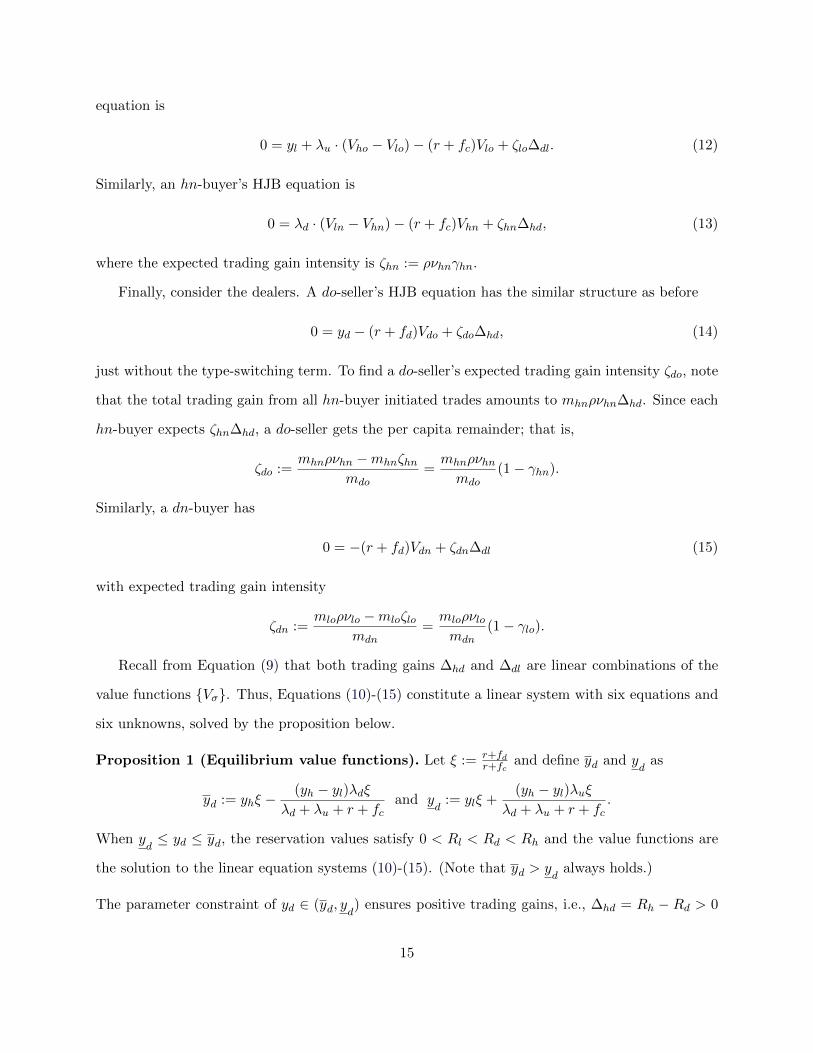
The contrasting effects between ρ and n can be seen most clearly from Figure 1(a) and 1(b),

which are based on parameters calibrated against the real-world RFQ trading of corporate bonds

(Appendix A). Specifically, while the intensity ρ always reduces the customer sizes, the effect of

the capacity n is more nuanced: It monotonically reduces mhn (the long side) but might increase

mlo (the short side). The proposition below sums up the patterns formally.

Proposition 2 (Search technology, customer sizes, and trading volume). The search in-

tensity ρ reduces both mhn and mlo. The search capacity n reduces the long-side customer mass

but has ambiguous effect on the short-side customer mass. In particular, when ρ is sufficiently

small, the short-side customer mass increases with n. The trading volume intensity t increases in

both n and ρ.

The proposition also states that both search technologies monotonically improve trading volume.

This is rather intuitive as the matching between customers and dealers become more efficient with

either higher ρ or larger n. Such increased trading volume, however, does not always translate to

allocation efficiency. Notably, a larger search capacity n might exacerbate inefficient allocation:

more low-type customers end up holding the asset. Indeed, the increase of mlo with n can be seen

along every horizontal cut in Figure 1(b), thought more saliently for lower than higher ρs. This is

“inefficient” as such holdings could have been better appreciated by high-type customers (as the

asset is in excess demand). As explained below, such inefficiency has a novel dealer “bottleneck”

effect to blame.

2.3.2 The bottleneck effect

Note that an increase in the search capacity n does help matching: Both the probabilities νlo

and νhn of finding at least one dealer counterparty increase with n, as can be seen from Figure 1(c)

and (d) (formally shown in Lemma S1.2 in the supplementary appendix). However, the magnitudes

of the increases are far from equal. The increment in νhn is much more substantial than that in

17

(a) Size of hn-buyers, mhn

100 101 102

Search capacity, n

10−1

100

101

102

Sear

chin

tens

ity,ρ

0.070

0.030

0.010

0.003

0.001

(b) Size of lo-sellers, mlo

100 101 102

Search capacity, n

10−1

100

101

102

Sear

chin

tens

ity,ρ

0.060

0.040

0.020

0.010

0.005

0.002

0.001

(c) Matching rate for an hn-buyer, νhn

100 101 102

Search capacity, n

10−1

100

101

102

Sear

chin

tens

ity,ρ

0.13

0.20

0.40

0.60

0.80

0.90

0.95

0.98

(d) Matching rate for an lo-seller, νlo

100 101 102

Search capacity, n

10−1

100

101

102

Sear

chin

tens

ity,ρ

0.70.8

0.9

0.950.99

0.9991−

10 −5

1−10 −

8

1−10 −

12

Figure 1: Customer sizes and matching rates. This figure plots how the search intensity ρ and the

search capacity n affect the customer sizes in (a) and (b) and the matching rates in (c) and (d). Apart

from ρ and n, the other parameters are set at s = 0.12, md = 0.10, λu = 0.04, and λd = 0.31, based

on the calibration exercise detailed in Appendix A. The other model parameters are irrelevant here as the

equilibrium demographics do not depend on them; see Equations (2)-(7) and Lemma 1.

18

νlo. This is because the lo-sellers are on the short side of the market and there are many more

dn-dealers to find (than do-dealers for the long side hn-buyers). Correspondingly, νlo is much closer

to its upper bound of 100% and cannot be increased by as much as νhn. Put differently, the increase

in n matches many more hn-do pairs than lo-dn pairs.

The lo-dn trades let the asset flow into the dealer sector, while the hn-do trades let the asset flow

out of the dealers. The above asymmetric effects of n—the substantially smaller inflow compared

to the outflow—imply that the asset flow is clogged when passing through the dealer sector, hence

the “bottleneck.”7 As the dealers give out a lot of the asset to hn-buyers but only take in little

from lo-sellers, the lo-seller size mlo increases and the hn-buyer size mhn reduces.

Summing up, there are two pairs of asymmetric effects: In terms of matching probability, νhn

increases much more than νlo. In terms of population sizes, mhn shrinks, whereas mlo balloons.

These effects ensure the stationarity of dealers in equilibrium, with ρνlomlo = ρνhnmhn (Equa-

tion 8). The above discussion is for the case of excess demand. When the asset is in excess supply,

the dealer bottleneck also arises as n increases: A substantially larger asset inflow than outflow

from the dealers raises both mdo and mhn, as the matching probability νlo increases much more

than νhn.

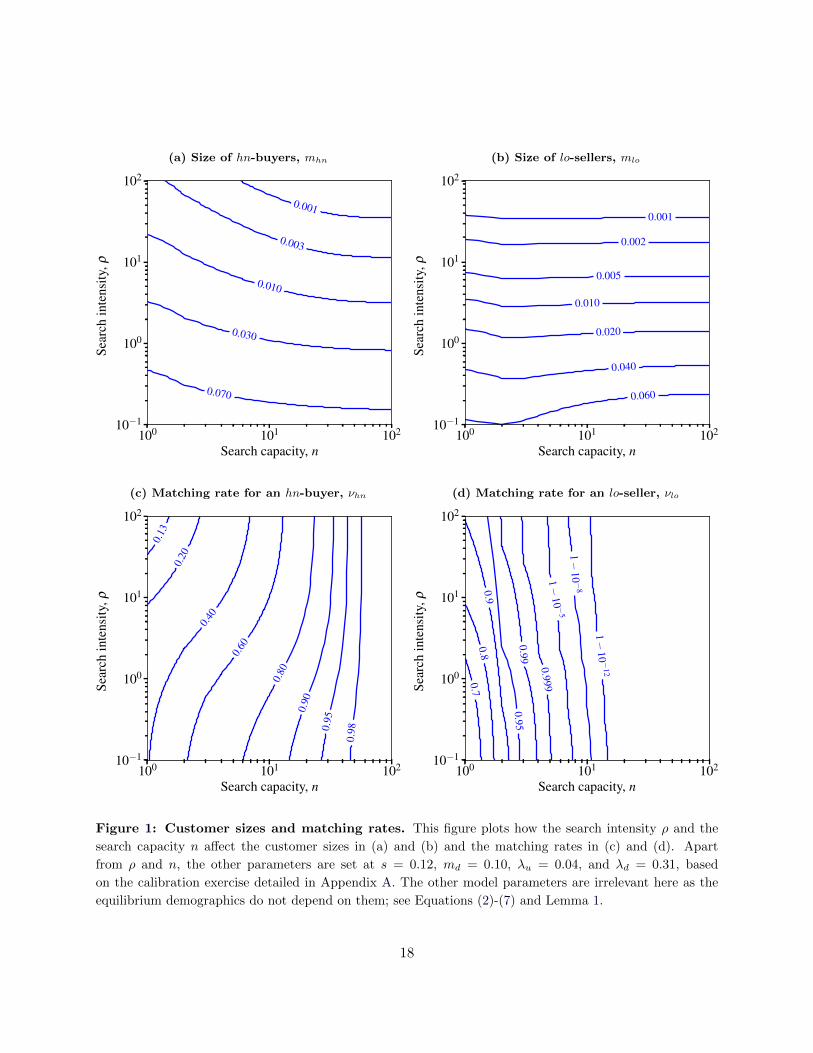
It is worth emphasizing that the bottleneck arises only with the search capacity n but not with

the intensity ρ. This is because ρ scales up both the inflow ρνlomlo and the outflow ρνhnmhn and

there is no asymmetry. This is a novel finding, thanks to the flexibility of n.8 For example, the

bottleneck does not manifest in HLW, as their customers and dealers only meet bilaterally (n = 1).

Proposition 2 emphasizes that the dealer bottleneck arises only when the search intensity ρ is

“low.” How “low” is low enough? To provide some perspective, Appendix A calibrates the model

parameters against the real-world RFQ trading of corporate bonds and finds robust presence of

7 The terminology of “bottleneck” also emphasizes that the inefficiency hinges on the existence of a sector ofdealers. Absent of such intermediaries, for example, the matching between the high-type and low-type customersalways results in the maximum trading gains, hence no inefficiency.

8 Supplementary Appendix S4 studies an extension of the model, where customers are allowed to endogenouslychoose their search intensity (subject to a flow cost). In equilibrium, lo-sellers search with ρlo, while hn-buyers with apossibly different ρhn. Numerically, such endogenously asymmetric ρs still create no dealer bottleneck. Our analysissuggests that this is because the search intensities still enter the stationarity condition proportionally on both sides:ρlomloνlo = ρhnmhnνhn. In contrast, the search capacity n asymmetrically affects the matching rates νlo and νhn(by exponentiating the intrinsically different matching probabilities πdn and πdo).

19

dealer bottlenecks, suggesting room for improving the efficiency of RFQ trading in practice.

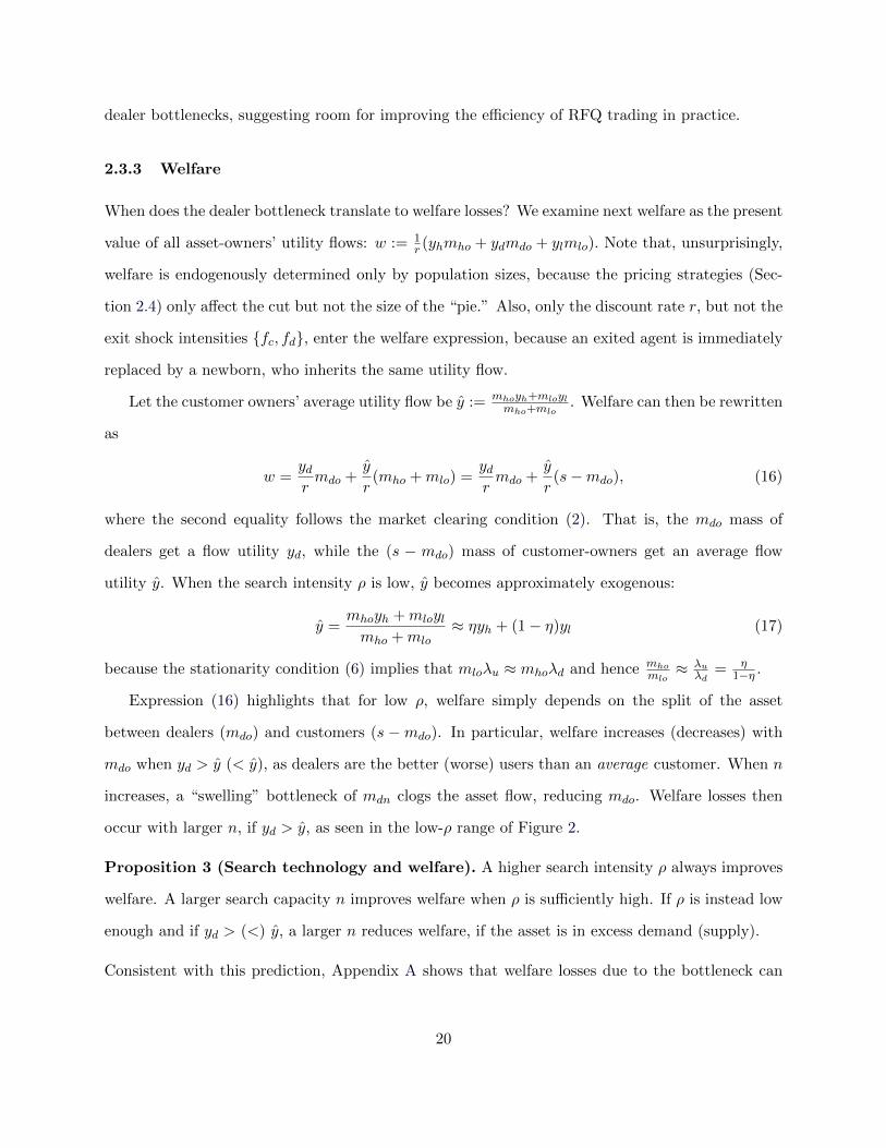
2.3.3 Welfare

When does the dealer bottleneck translate to welfare losses? We examine next welfare as the present

value of all asset-owners’ utility flows: w := 1r (yhmho + ydmdo + ylmlo). Note that, unsurprisingly,

welfare is endogenously determined only by population sizes, because the pricing strategies (Sec-

tion 2.4) only affect the cut but not the size of the “pie.” Also, only the discount rate r, but not the

exit shock intensities {fc, fd}, enter the welfare expression, because an exited agent is immediately

replaced by a newborn, who inherits the same utility flow.

Let the customer owners’ average utility flow be y := mhoyh+mloylmho+mlo

. Welfare can then be rewritten

as

w =ydrmdo +

y

r(mho +mlo) =

ydrmdo +

y

r(s−mdo), (16)

where the second equality follows the market clearing condition (2). That is, the mdo mass of

dealers get a flow utility yd, while the (s − mdo) mass of customer-owners get an average flow

utility y. When the search intensity ρ is low, y becomes approximately exogenous:

y =mhoyh +mloylmho +mlo

≈ ηyh + (1− η)yl (17)

because the stationarity condition (6) implies that mloλu ≈ mhoλd and hence mhomlo

≈ λuλd

= η1−η .

Expression (16) highlights that for low ρ, welfare simply depends on the split of the asset

between dealers (mdo) and customers (s −mdo). In particular, welfare increases (decreases) with

mdo when yd > y (< y), as dealers are the better (worse) users than an average customer. When n

increases, a “swelling” bottleneck of mdn clogs the asset flow, reducing mdo. Welfare losses then

occur with larger n, if yd > y, as seen in the low-ρ range of Figure 2.

Proposition 3 (Search technology and welfare). A higher search intensity ρ always improves

welfare. A larger search capacity n improves welfare when ρ is sufficiently high. If ρ is instead low

enough and if yd > (<) y, a larger n reduces welfare, if the asset is in excess demand (supply).

Consistent with this prediction, Appendix A shows that welfare losses due to the bottleneck can

20

100 101 102

Search capacity, n

10−1

100

101

102

Sear

chin

tens

ity,ρ

1.0

1.5

2.0

2.2

2.3

2.4

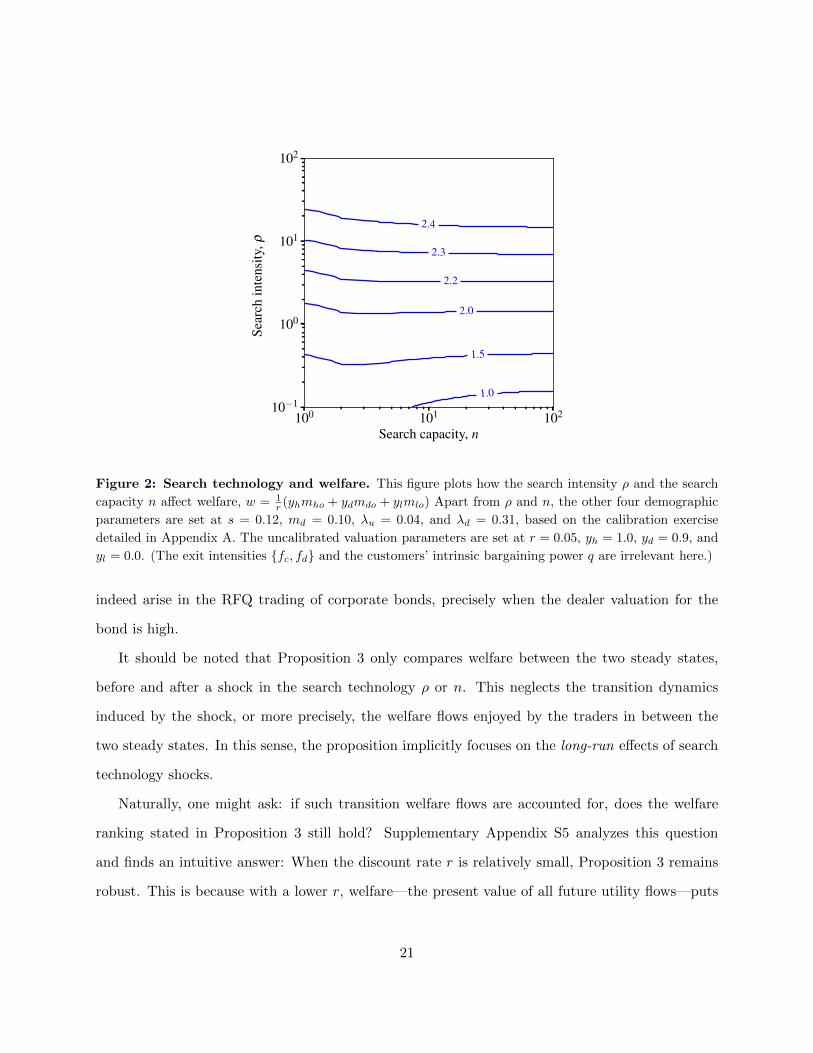
Figure 2: Search technology and welfare. This figure plots how the search intensity ρ and the search

capacity n affect welfare, w = 1r (yhmho + ydmdo + ylmlo) Apart from ρ and n, the other four demographic

parameters are set at s = 0.12, md = 0.10, λu = 0.04, and λd = 0.31, based on the calibration exercise

detailed in Appendix A. The uncalibrated valuation parameters are set at r = 0.05, yh = 1.0, yd = 0.9, and

yl = 0.0. (The exit intensities {fc, fd} and the customers’ intrinsic bargaining power q are irrelevant here.)

indeed arise in the RFQ trading of corporate bonds, precisely when the dealer valuation for the

bond is high.

It should be noted that Proposition 3 only compares welfare between the two steady states,

before and after a shock in the search technology ρ or n. This neglects the transition dynamics

induced by the shock, or more precisely, the welfare flows enjoyed by the traders in between the

two steady states. In this sense, the proposition implicitly focuses on the long-run effects of search

technology shocks.

Naturally, one might ask: if such transition welfare flows are accounted for, does the welfare

ranking stated in Proposition 3 still hold? Supplementary Appendix S5 analyzes this question

and finds an intuitive answer: When the discount rate r is relatively small, Proposition 3 remains

robust. This is because with a lower r, welfare—the present value of all future utility flows—puts

21

(a) Welfare

0.5 0.6 0.7 0.8 0.9 1.0

0

−10

−20

−30

−40

Welfare loss (relative to ψ = 0.5, basis points)

Transparency, ψ

(b) Matching rates

0.5 0.6 0.7 0.8 0.9 1.0

92

94

96

98

100νlo (solid) and νhn (dashed), %

Transparency, ψ

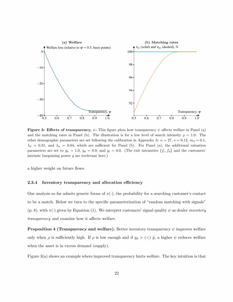
Figure 3: Effects of transparency, ψ. This figure plots how transparency ψ affects welfare in Panel (a)

and the matching rates in Panel (b). The illustration is for a low level of search intensity ρ = 1.0. The

other demographic parameters are set following the calibration in Appendix A: n = 27, s = 0.12, md = 0.1,

λd = 0.31, and λu = 0.04, which are sufficient for Panel (b). For Panel (a), the additional valuation

parameters are set to yh = 1.0, yd = 0.9, and yl = 0.0. (The exit intensities {fc, fd} and the customers’

intrinsic bargaining power q are irrelevant here.)

a higher weight on future flows.

2.3.4 Inventory transparency and allocation efficiency

Our analysis so far admits generic forms of π(·), the probability for a searching customer’s contact

to be a match. Below we turn to the specific parameterization of “random matching with signals”

(p. 8), with π(·) given by Equation (1). We interpret customers’ signal quality ψ as dealer inventory

transparency and examine how it affects welfare.

Proposition 4 (Transparency and welfare). Better inventory transparency ψ improves welfare

only when ρ is sufficiently high. If ρ is low enough and if yd > (<) y, a higher ψ reduces welfare

when the asset is in excess demand (supply).

Figure 3(a) shows an example where improved transparency hurts welfare. The key intuition is that

22

the change in transparency ψ asymmetrically affects customers on the short and the long sides of

the market, similar to the asymmetric effects of n in Section 2.3. A higher ψ improves matching by

increasing both νhn and νlo, helping customers direct more accurately their searches to dealers with

the right inventory capacity. Yet, the short side matching rate (νlo) increases much less than the

long side (νhn), since it is already close to the upper bound of 100%, as illustrated in Figure 3(b).

(In fact, νlo is too close to 100% to begin with, making it almost flat in the illustration.) The

bottleneck again emerges and possibly hurts welfare, mirroring Proposition 3.

The dissemination of post-trade information of corporate bonds via TRACE (Transaction Re-

porting and Compliance Engine), starting in 2002, was perhaps the most significant transparency

shock in the corporate bonds market. A large volume of the literature has documented its impact

on market quality, applauding the improved liquidity and the reduced trading costs (e.g., Bessem-

binder, Maxwell, and Venkataraman, 2006, Edwards, Harris, and Piwowar, 2007, and, Goldstein,

Hotchkiss, and Sirri, 2007). The extant theory models also seem to agree that welfare always im-

proves with inventory transparency (e.g., Cujean and Praz, 2015, who study bilateral searches by

customers, without going through a dealer sector). To the extent that post-trade transparency from

TRACE also improves customers’ inference about dealer inventories, our model cautions that the

resulting better matching—the improved “liquidity”—not necessarily always translates to better

welfare in terms of allocation (Figure 3a vs. 3b). In particular, our model highlights the importance

of empirically examining how dealer inventories respond to such transparency shocks.

2.4 The endogenous split of trading gain

The analysis so far only requires the general form of expected trading gain shares, {γhn, γlo}. Under

the assumed trading mechanism (“Price determination” on p. 8), such expected trading gain shares

can be endogenously determined:

Proposition 5 (The split of trading gains). Define γ(π, n) := q+ (1− q)(1− nπ·(1−π)n−1

1−(1−π)n

)for

π ∈ (0, 1) and n ∈ N. Then, γhn = γ(πdo, n) and γlo = γ(πdn, n).

This proposition thus completes the equilibrium characterization. Several features are worth dis-

cussing. First, as long as n ≥ 2, γ(·) is strictly increasing in π, from γ(0, n) = q to γ(1, n) = 1.

23

Take, for example, an hn-buyer searching for do-dealers. With a higher πdo, each contacted do-

dealer knows that she is more likely competing with some other do-dealers among the other (n−1)

contacts. Such fiercer competition gives more trading gains to the hn-buyer. Indeed, when πdo → 1,

hn-buyers extract full surplus with γhn → 1 from the dealers’ perfect competition. On the other

extreme, if πdo → 0, each do-dealer knows that she is likely the monopolist among all n contacted

and therefore quotes a monopolistic price. Indeed, as πdo → 0, γhn → q, which is the baseline

probability that the customer can make TIOLIOs to the contacted dealers.

Second, when n = 1, γhn = γlo = q, as if the searching customer engages in a Nash bargaining

with one matched dealer with respective bargaining power parameters q and 1 − q. Our setup

thus nests such exogenous splits of trading gains, commonly assumed in the literature (see, e.g.,

DGP and HLW). When n ≥ 2, our model highlights that under SMS, the expected trading gain

shares {γhn, γlo} are endogenous, in particular, of the dealer composition mdo and mdn. Such an

endogenous split of trading gains is a distinguishing feature of our model.

Finally, whenever n ≥ 2, the contacted dealers compete against an unknown number of others,

as some of the n contacted dealers might not be of the matching type. That is, every contacted

matching dealer knows that there is a non-zero probability that she actually is the only match.

As is known in the literature (e.g., Burdett and Judd, 1983), in this case, dealers follow mixed

strategies in setting their prices. This suggests that dealers’ strategic behavior can be a source

of price dispersion. Even though dealers are homogeneous in our model, it still features price

dispersion, a robust empirical feature of OTC markets. For example, Hendershott and Madhavan

(2015) document a significant dispersion in dealers’ responding quotes in corporate bond market.

Hau et al. (2017) find evidence for price dispersion in foreign exchange derivatives.

Corollary 5 only characterizes the split of trading gains. The implied γ(π, n) also feed back to

the equilibrium price formation in terms of dealers’ quotes, the average price level in the economy,

and the price dispersion. Supplementary Appendix S3 detail these results regarding the price.

24

3 SMS versus BB: How to search

In real-world trading, investors can choose their trading technologies. For example, while bilateral

bargaining is still the dominant form of trading in corporate bonds, electronic platforms with RFQ

protocols have been on the rise (O’Hara and Zhou, 2021). We consider investors’ choice of “Click

or Call” (Hendershott and Madhavan, 2015) in this section.

Specifically, we introduce two technologies, BB and SMS. They differ in parameters {nk, ρk, qk},

k ∈ {BB, SMS} (some realistic parameter restrictions are imposed below). Each customer can

choose, at any point in time, which technology to use to contact dealers, if she wants to trade. All

dealers can be reached either by BB or by SMS. The other model ingredients remain the same as

in Section 1.

Section 3.1 analyzes how customers choose between the two technologies in a steady state

equilibrium. We then examine whether SMS-like electronic trading (e.g., RFQ) can completely

replace traditional bilateral bargaining. The answer is no, as Section 3.2 shows that in stress periods

(e.g., after a fire sale), BB is used more often than SMS. Finally, Section 3.3 draws implications on

welfare, policy, and market design.

Parameter constraints. Motivated by “calls” (BB) and “clicks” (SMS), we assume

nBB = 1, nSMS > 2, and ρBB ≤ ρSMS. (18)

In a bilateral call, a customer bargains with one dealer, hence nBB = 1. By clicking, a typical

real-world RFQ protocol connects the customer to multiple dealers, at least three in most of the

applications (see Remark 3), hence nSMS > 2.9 Earlier research finds that electronic platforms

can “provide considerable time savings relative to ... bilateral negotiations” (Hendershott and

Madhavan, 2015); and can “improve the speed of execution” (O’Hara and Zhou, 2021), motivating

ρBB ≤ ρSMS.

The probabilities to set prices in respective technology, qBB and qSMS, also play an important

role. In most of the applications (e.g., MarketAxess), a customer using RFQ is always on the

9 Excluding the special case of nSMS = 2 reduces the cases to consider when characterizing the equilibrium,streamlining the exposition. The full characterization for nSMS ≥ 2 is provided in the proof of Proposition 6.

25

receiving end of dealers’ TIOLIOs, suggesting that qSMS = 0. On the other hand, in bilateral calls,

there is always room for negotiation and it is natural to expect that qBB > 0. We impose no

such constraints here and proceed to examine how qSMS and qBB affect the customers’ technology

choices.

3.1 Choosing between SMS and BB

As before, we only focus on steady states, characterized by three sets of equilibrium objects: (i)

customers’ optimal technology choices, (ii) demographics, and (iii) value functions. Compared to

Section 2, the novel part is the analysis of (i), detailed below. The analyses of (ii) and (iii) are

analogous to those in Section 2 and, hence, collated in Supplementary Appendix S1.2-S1.3.

Recall from Section 1 that there are four types of customers, σ ∈ {ho, ln, hn, lo}. Now the

σ-type customers can be further split into subtypes σ-BB and σ-SMS, which we distinguish by

superscripting the relevant variables with the chosen technology k ∈ {BB,SMS}. For example,

their masses satisfy mBBσ +mSMS

σ = mσ and they have (possibly different) value functions V BBσ and

V SMSσ .

The analysis can be simplified in two ways. First, note that in a stationary equilibrium, the

value functions are time-invariant. That is, if a type-σ customer prefers one technology over the

other at some point of time, her technology choice will persist until her type changes (due either

to a preference shock or to trading). Hence, without loss of generality, we can focus on a type-σ

customer’s technology choice at the moment she becomes type-σ. Second, both ho and ln customers

will be bystanders in equilibrium, just like in the case of one trading technology before. Therefore,

there is no need to distinguish lnSMS versus lnBB or hoSMS versus hoBB. Only the technology

choices of the trading customers, hn and lo, need to be studied below.

Denote by θσ ∈ [0, 1] the probability of a customer, who just received a preference shock and

becme type-σ, to choose SMS (hence choosing BB with probability 1 − θσ), where σ ∈ {hn, lo}.

26

Then

θσ

= 1{V SMS

σ >V BBσ }, if V SMS

σ = V BBσ ;

∈ [0, 1], if V SMSσ = V BB

σ .

(19)

We shall focus on symmetric equilibria, where all customers of type σ choose the same θσ.

To sustain an equilibrium, the technology choices {θhn, θlo} must agree with the value func-

tions {Vσ} according to Equation (19). The value functions are, in turn, chained to {θhn, θlo}

via many layers of endogenous variables (see Supplementary Appendix S1.3): the trading gain

intensities {ζσ}, the dealers’ pricing, and the many demographic variables {mσ}— a big fixed-

point problem. It turns out that the equilibrium {θhn, θlo} ultimately boil down to comparing the

probabilities of finding a match, i.e., πdo = π(mdomd

)and πdn = π

(mdnmd

), with some threshold π∗:

Lemma 3. If the technologies satisfy

ρSMSqSMSnSMS < ρBBqBBnBB, (20)

then Equation (19) can be equivalently written as

θhn

= 1{πdo>π∗}, if πdo = π∗

∈ [0, 1], if πdo = π∗and θlo

= 1{πdn>π∗}, if πdn = π∗

∈ [0, 1], if πdn = π∗, (21)

where π∗ uniquely solves zSMS(π) = zBB(π), with zk(·) defined in Equation (23) below for k ∈

{SMS,BB}. If, instead, ρSMSqSMSnSMS ≥ ρBBqBBnBB, then θhn = θlo = 1.

Below we discuss the key steps behind this lemma. First, the value functions are pinned down

by the HJB equations (S11)-(S14) in Supplementary Appendix S1.3. The proof of Lemma 3 shows

that V kσ is a monotone function in ζkσ , for σ ∈ {lo, hn}. This intuitive result says that when a

searching customer chooses between SMS vs. BB, she is essentially comparing the trading gain

intensities ζSMSσ vs. ζBB

σ . Hence, the technology choices (19) can be equivalently written as:

θσ

= 1{ζSMS

σ >ζBBσ }, if ζSMS

σ = ζBBσ ;

∈ [0, 1], if ζSMSσ = ζBB

σ .

(22)

Second, analogous to {ζlo, ζhn} in Section 2.2, we write ζkhn = zk(πdo) and ζklo = zk(πdn), where

27

zk(·) is defined for π ∈ (0, 1) as

zk(π) := ρkνk(π)γk(π) = ρk ·(1− (1− π)n

k)(

qk + (1− qk)

(1− nkπ · (1− π)n

k−1

1− (1− π)nk

)). (23)

The superscript k is not exponent but indicates the technology k ∈ {BB,SMS}. That is, customers

essentially choose {θσ} by examining whether and how zSMS(π) and zBB(π) cross each other.

Lemma 3 essentially characterizes such crossing. Under the condition (20), zSMS(π) crosses

zBB(π) from below once at π∗ ∈(0, 12). That is, a hn-buyer (lo-seller) prefers BB over SMS when

πdo < π∗ (πdn < π∗). This might come as a surprise, given that the condition (18) has guaranteed

that SMS not only helps reach dealers faster but also induces more competitive quotes. Why would

a customer still prefer BB?

To see the potential advantage of BB, consider for example an hn-buyer looking for do-sellers.

Suppose mdo is very low and, hence, so is πdo = π(mdomd

). Then the hn-buyer customer finds

one counterparty dealer with probability approximately nkπdo—one and only one success from nk

Bernoulli draws at rate πdo. (For small πdo, finding multiple dealers is negligibly unlikely.) It follows

that a successfully contacted dealer in this case knows that she is almost surely a monopolist and

will quote a very expensive ask, leaving no trading gain to the hn-buyer. The customer only gets

non-zero trading gain if she can make a TIOLIO, i.e., with probability qk. Taken together, for

small π, the customers’ trading gain intensity is zk(π) ≈ ρk · (nkπ) · qk. Comparing BB with SMS

in this case yields:

limπ↓0

zBB(π)

zSMS(π)=

ρBBnBBqBB

ρSMSnSMSqSMS.

The condition (20), therefore, ensures that for sufficiently small π, i.e., for relatively few counter-

party dealers, BB has an advantage over SMS. In real-world trading, the condition (20) seems to

hold because customers using SMS, like RFQ protocols, do not have many opportunities, if at all,

to further bargain with dealers. We, therefore, argue that qSMS is close to zero in reality.10

10 Complementing the condition (20), the condition (18) in turn ensures that SMS is preferred when there aresufficiently many dealer counterparties.That is, limπ↑1

(zBB(π)/zSMS(π)

)= ρBBqBB/ρSMS ≤ 1. It is interesting to

note that only qBB appears but not qSMS in the limit of π ↑ 1. With nSMS > 1 and π ↑ 1, the multiple counterpartydealers in SMS almost always engage in Bertrand competition, and the customer always gets the full trading gain,regardless of qSMS. On the contrary, with nBB = 1, a customer using BB meets only one counterparty dealer, whowill always set the monopolist price, leaving surplus to the customer only with probability qBB.

28

We are now ready to state the equilibrium.

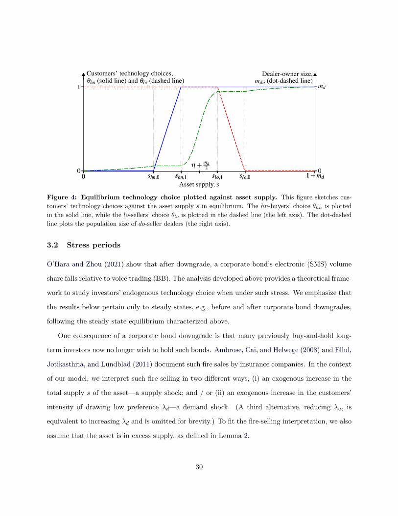
Proposition 6 (Steady state equilibrium with technology choices). A unique stationary

equilibrium exists depending on the asset supply s: There exist thresholds 0 < shn,0 < shn,1 ≤

slo,1 < slo,0 < 1 +md so that(a) hn-buyers’ proba-bility to use SMS, θhn

(b) lo-sellers’ proba-bility to use SMS, θlo

(c) asset holdingby dealers, mdo

(1) 0 < s ≤ shn,0 0 1 g(0, 1,mdo) = s

(2) shn,0 ≤ s ≤ shn,1 g(θhn, 1,m∗d) = s 1 m∗

d

(3) shn,1 < s < slo,1 1 1 g(1, 1,mdo) = s

(4) slo,1 ≤ s ≤ slo,0 1 g(1, θlo,md −m∗d) = s md −m∗

d

(5) slo,0 < s < 1 +md 1 0 g(1, 0,mdo) = s

where g(x1, x2, x3) = s uniquely solves θhn, θlo, and mdo in columns (a), (b), and (c), respec-

tively. The constant π∗ is given in Lemma 3 and m∗d := π−1(π∗)md. The function g(·) and the

thresholds {shn,0, shn,1, slo,1, slo,0} are given in the proof. As a special case, when ρSMSqSMSnSMS ≥

ρBBqBBnBB, the thresholds collapse to shn,0 = shn,1 = 0 and slo,0 = slo,1 = 1 + md, and the

equilibrium is described by (3) of the above table, consistent with Lemma 3.

Figure 4 illustrates the equilibrium by plotting the technology choices θhn (solid) and θlo (dashed)

on the left axis and the dealer-owner population size mdo (dot-dashed) on the right axis. The

four thresholds of {shn,0, shn,1, slo,1, slo,0} cut the support of s ∈ (0, 1 + md) into five regions on

the horizontal axis. Consider the solid line, i.e., θhn, for example. When the asset supply s is

extremely low, SMS is very unattractive for the hn-buyers, because they know it is very difficult

to find a counterparty do-dealer (the dot-dashed line), and even if they do, they are going to

be charged with a monopoly price using SMS. When s is sufficiently high, there are sufficiently

many do-dealers, whose price competition makes SMS sufficiently attractive with high trading gain

intensity ζSMShn for hn-buyers. As such, the solid line flattens at θhn = 1 for s > shn,1. In between,

we see θhn monotonically increases for shn,0 ≤ s ≤ shn,1. Such a mixed strategy is supported by the

constant mdo = π∗md in the region—the hn-buyers are indifferent to BB and SMS. The pattern

for the dashed line, i.e., θlo, is exactly the opposite, as lo-sellers seek dn-dealers, whose mass is

mdn = md −mdo.

29

0 shn,0 shn,1 slo,1 slo,0 1+md

Asset supply, s

0

1

η + md2

Customers’ technology choices,θhn (solid line) and θlo (dashed line)

0 shn,0 shn,1 slo,1 slo,0 1+md0

md

Dealer-owner size,mdo (dot-dashed line)

Figure 4: Equilibrium technology choice plotted against asset supply. This figure sketches cus-

tomers’ technology choices against the asset supply s in equilibrium. The hn-buyers’ choice θhn is plotted

in the solid line, while the lo-sellers’ choice θlo is plotted in the dashed line (the left axis). The dot-dashed

line plots the population size of do-seller dealers (the right axis).

3.2 Stress periods

O’Hara and Zhou (2021) show that after downgrade, a corporate bond’s electronic (SMS) volume

share falls relative to voice trading (BB). The analysis developed above provides a theoretical frame-

work to study investors’ endogenous technology choice when under such stress. We emphasize that

the results below pertain only to steady states, e.g., before and after corporate bond downgrades,

following the steady state equilibrium characterized above.

One consequence of a corporate bond downgrade is that many previously buy-and-hold long-

term investors now no longer wish to hold such bonds. Ambrose, Cai, and Helwege (2008) and Ellul,

Jotikasthria, and Lundblad (2011) document such fire sales by insurance companies. In the context

of our model, we interpret such fire selling in two different ways, (i) an exogenous increase in the

total supply s of the asset—a supply shock; and / or (ii) an exogenous increase in the customers’

intensity of drawing low preference λd—a demand shock. (A third alternative, reducing λu, is

equivalent to increasing λd and is omitted for brevity.) To fit the fire-selling interpretation, we also

assume that the asset is in excess supply, as defined in Lemma 2.

30

(a) Supply shock on s

η + md2 slo,1 slo,0 1+md

50

60

70

80

90

100SMS volume relative to total volume, %

Asset supply, s

(b) Demand shock on λd

50

60

70

80

90

100SMS volume relative to total volume, %

Intensity for lowcustomer preference, λd

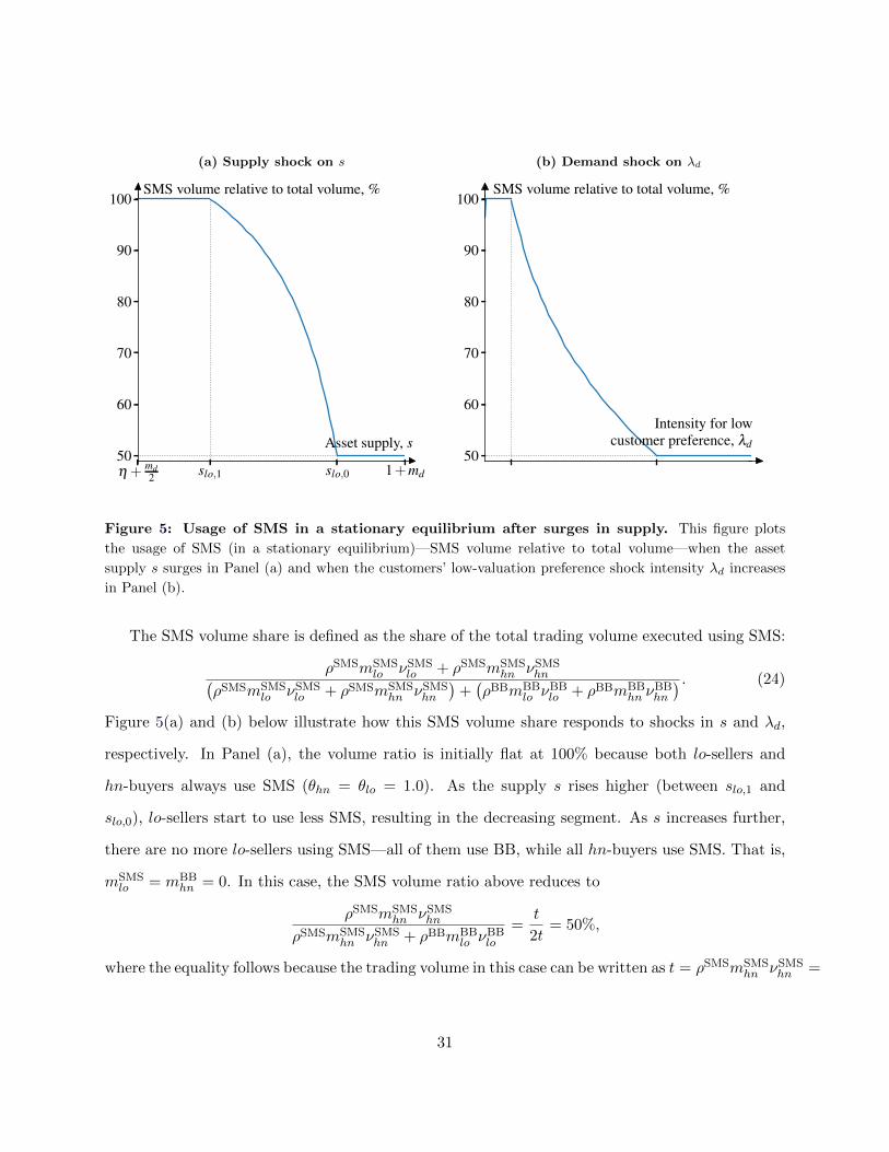
Figure 5: Usage of SMS in a stationary equilibrium after surges in supply. This figure plots

the usage of SMS (in a stationary equilibrium)—SMS volume relative to total volume—when the asset

supply s surges in Panel (a) and when the customers’ low-valuation preference shock intensity λd increases

in Panel (b).

The SMS volume share is defined as the share of the total trading volume executed using SMS:

ρSMSmSMSlo νSMS

lo + ρSMSmSMShn νSMS

hn(ρSMSmSMS

lo νSMSlo + ρSMSmSMS

hn νSMShn

)+(ρBBmBB

lo νBBlo + ρBBmBB

hn νBBhn

) . (24)

Figure 5(a) and (b) below illustrate how this SMS volume share responds to shocks in s and λd,

respectively. In Panel (a), the volume ratio is initially flat at 100% because both lo-sellers and

hn-buyers always use SMS (θhn = θlo = 1.0). As the supply s rises higher (between slo,1 and

slo,0), lo-sellers start to use less SMS, resulting in the decreasing segment. As s increases further,

there are no more lo-sellers using SMS—all of them use BB, while all hn-buyers use SMS. That is,

mSMSlo = mBB

hn = 0. In this case, the SMS volume ratio above reduces to

ρSMSmSMShn νSMS

hn

ρSMSmSMShn νSMS

hn + ρBBmBBlo ν

BBlo

=t

2t= 50%,

where the equality follows because the trading volume in this case can be written as t = ρSMSmSMShn νSMS

hn =

31

ρBBmBBlo ν

BBlo . Overall, the SMS volume ratio drops with the decline of the SMS usage θlo, as seen

before in Figure 4. The same pattern is observed from Panel (b), where we increase the customers’

negative preference shock intensity λd, effectively reducing the demand for the asset.

Proposition 7 (SMS usage under stress). The usage of SMS decreases with either the asset’s

excess supply or with its excess demand. That is, all else equal, for s > shn,1 (< slo,0), the ratio

defined in (24) weakly decreases when s increases (decreases) or when λd increases (decreases).

The proposition also gives the mirroring result: SMS usage also drops when the asset’s excess

demand exacerbates (s < η + md2 ).

The key intuition for the decrease of the SMS volume share can be understood from the wors-

ening pricing for the lo-sellers. As the asset supply s increases after the fire sell, there are more and

more do-dealers, as shown in the dot-dashed line in Figure 4. This is also evidenced empirically

by Anand, Jotikasthira, and Venkataraman (2021), who show that the majority of dealers enter a

positive inventory cycle upon a corporate bond’s downgrade (e.g., their Figure 2C). The remaining

dn-dealers, facing less competition, therefore, will charge worse and worse prices to the lo-sellers in

SMS. Expecting such worsening prices from SMS, the lo-sellers then avoid using SMS and switch

to BB. In particular, our model yields an additional prediction regarding prices in SMS and in BB

under a fire sell:

Proposition 8 (Prices in SMS versus in BB under fire sell). When there is excess supply,

an lo-seller’s expected trading price using SMS worsens relative to using BB.

Therefore, one way to empirically test our theory is to compare the trading prices in BB and in

SMS when the asset is under fire sell and examine if the price in SMS is worse than that in BB.

To compare, Hendershott and Madhavan (2015) also shed light on customers’ choice between

“call” and “click.” There the key disadvantage of SMS (click) is the leakage of one’s private

information to the multiple contacted dealers, as opposed to the only one in BB (call). Our

mechanism complements theirs by explaining the volume shift to BB after shocks not affecting

information asymmetry, such as corporate bond downgrades.

32

3.3 Efficiency and welfare

Are the market’s equilibrium technology choices socially optimal? Given the technologies {nk, ρk, qk},

how would a social planner choose {θlo, θhn} for the customers? When, if at all, do the market’s

equilibrium choices {θlo, θhn} coincide with the planner’s {θ∗lo, θ∗hn}?

The answers critically depend on the characteristics of the asset. Among others, how quickly

customers can find dealers, i.e., {ρBB, ρSMS}, matters a lot. Recall from the technology assump-

tion (18) that ρBB ≤ ρSMS. Therefore, it suffices to consider the cases of high-ρBB and the low-ρSMS

below.

3.3.1 The case of high search intensity

Proposition 9 (A social planner’s technology choices, I). When the search intensity ρBB

(≤ ρSMS) is sufficiently high, welfare w is monotone increasing in SMS usages by both types of

customers and the social planner chooses θ∗lo = θ∗hn = 1.

The intuition largely follows Proposition 3. When the search intensity is high, Proposition 3 shows

that welfare is monotone increasing in n. As such, by assigning both θ∗lo = θ∗hn = 1, the planner

chooses nSMS over nBB to maximize welfare.

However, the market’s technology choices do not always coincide with the planner’s. This is

because a customer cares not only about the probability of finding a counterparty dealer but also

about the endogenous split of the trading gain. Figure 6 sketches such possible discrepancies. The

solid line and the dashed line plot, respectively, the market’s choices of θhn and θlo against the

asset supply s. (Note that the patterns are qualitatively the same as in Figure 4.) The shaded

areas indicate that there is inefficiency in the market’s technology choices. For example, when the

excess supply s is relatively extreme, s > slo,1, as in fire sell (Section 3.2), the dealer sector becomes

overloaded (mdo too large), giving lo-sellers a hard time finding dn-dealers. Then lo-sellers become

less willing to use SMS (θlo decreases with s) because in SMS their trading gains are too low. The

same holds when s < shn,1 (extreme excess demand).

Since the planner wants to encourage SMS usage, a simple, welfare-improving market design

mandate readily follows: Let customers indicate their reservation values when searching dealers via

33

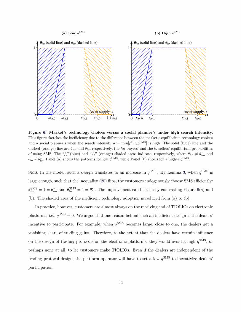
(a) Low qSMS

0 shn,0 shn,1 slo,1 slo,0 1+md0

1θhn (solid line) and θlo (dashed line)

Asset supply, s

(b) High qSMS

0 shn,0 shn,1 slo,1 slo,00

1θhn (solid line) and θlo (dashed line)

Asset supply, s

Figure 6: Market’s technology choices versus a social planner’s under high search intensity.

This figure sketches the inefficiency due to the difference between the market’s equilibrium technology choices

and a social planner’s when the search intensity ρ := min[ρBB, ρSMS] is high. The solid (blue) line and the

dashed (orange) line are θhn and θlo, respectively, the hn-buyers’ and the lo-sellers’ equilibrium probabilities

of using SMS. The “//”(blue) and “\\” (orange) shaded areas indicate, respectively, where θhn = θ∗hn and

θlo = θ∗lo. Panel (a) shows the patterns for low qSMS, while Panel (b) shows for a higher qSMS.

SMS. In the model, such a design translates to an increase in qSMS. By Lemma 3, when qSMS is

large enough, such that the inequality (20) flips, the customers endogenously choose SMS efficiently:

θSMShn = 1 = θ∗hn and θSMS

lo = 1 = θ∗lo. The improvement can be seen by contrasting Figure 6(a) and

(b): The shaded area of the inefficient technology adoption is reduced from (a) to (b).

In practice, however, customers are almost always on the receiving end of TIOLIOs on electronic

platforms; i.e., qSMS = 0. We argue that one reason behind such an inefficient design is the dealers’

incentive to participate. For example, when qSMS becomes large, close to one, the dealers get a

vanishing share of trading gains. Therefore, to the extent that the dealers have certain influence

on the design of trading protocols on the electronic platforms, they would avoid a high qSMS, or

perhaps none at all, to let customers make TIOLIOs. Even if the dealers are independent of the

trading protocol design, the platform operator will have to set a low qSMS to incentivize dealers’

participation.

34

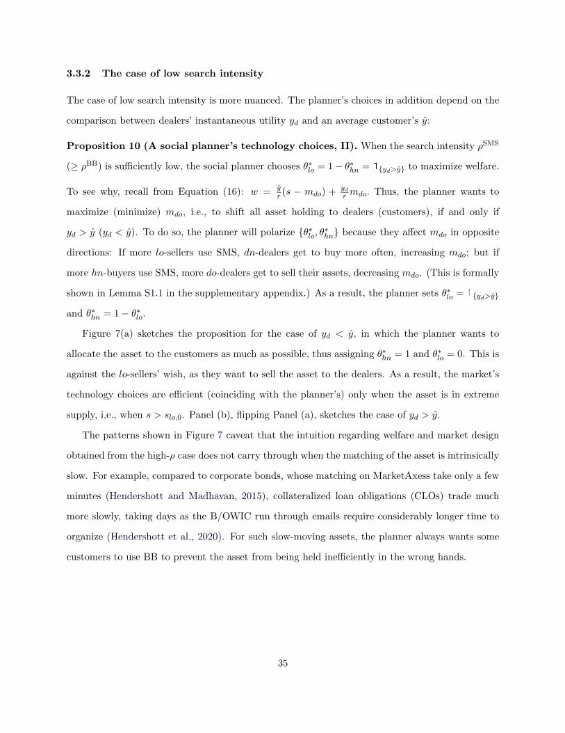
3.3.2 The case of low search intensity

The case of low search intensity is more nuanced. The planner’s choices in addition depend on the

comparison between dealers’ instantaneous utility yd and an average customer’s y:

Proposition 10 (A social planner’s technology choices, II). When the search intensity ρSMS

(≥ ρBB) is sufficiently low, the social planner chooses θ∗lo = 1− θ∗hn = 1{yd>y} to maximize welfare.

To see why, recall from Equation (16): w = yr (s − mdo) +

ydr mdo. Thus, the planner wants to

maximize (minimize) mdo, i.e., to shift all asset holding to dealers (customers), if and only if

yd > y (yd < y). To do so, the planner will polarize {θ∗lo, θ∗hn} because they affect mdo in opposite

directions: If more lo-sellers use SMS, dn-dealers get to buy more often, increasing mdo; but if

more hn-buyers use SMS, more do-dealers get to sell their assets, decreasing mdo. (This is formally

shown in Lemma S1.1 in the supplementary appendix.) As a result, the planner sets θ∗lo = 1{yd>y}

and θ∗hn = 1− θ∗lo.

Figure 7(a) sketches the proposition for the case of yd < y, in which the planner wants to

allocate the asset to the customers as much as possible, thus assigning θ∗hn = 1 and θ∗lo = 0. This is

against the lo-sellers’ wish, as they want to sell the asset to the dealers. As a result, the market’s

technology choices are efficient (coinciding with the planner’s) only when the asset is in extreme

supply, i.e., when s > slo,0. Panel (b), flipping Panel (a), sketches the case of yd > y.

The patterns shown in Figure 7 caveat that the intuition regarding welfare and market design

obtained from the high-ρ case does not carry through when the matching of the asset is intrinsically

slow. For example, compared to corporate bonds, whose matching on MarketAxess take only a few

minutes (Hendershott and Madhavan, 2015), collateralized loan obligations (CLOs) trade much

more slowly, taking days as the B/OWIC run through emails require considerably longer time to

organize (Hendershott et al., 2020). For such slow-moving assets, the planner always wants some

customers to use BB to prevent the asset from being held inefficiently in the wrong hands.

35

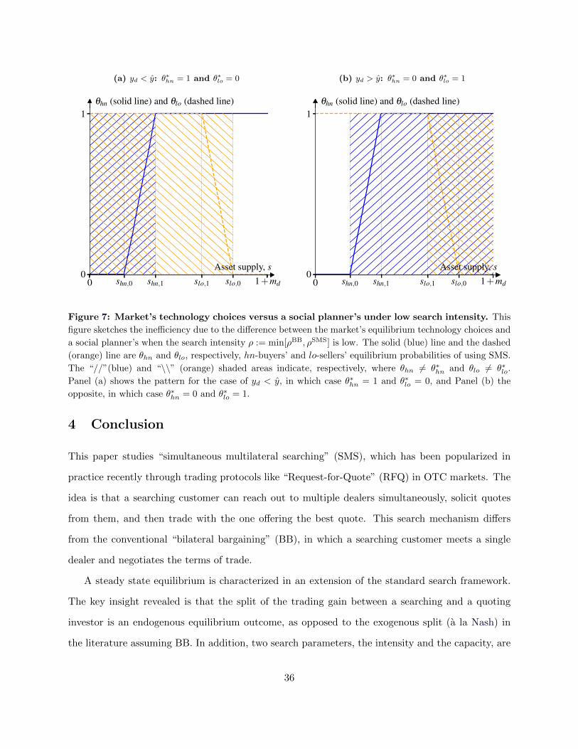
(a) yd < y: θ∗hn = 1 and θ∗lo = 0

0 shn,0 shn,1 slo,1 slo,0 1+md0

1θhn (solid line) and θlo (dashed line)

Asset supply, s

(b) yd > y: θ∗hn = 0 and θ∗lo = 1

0 shn,0 shn,1 slo,1 slo,0 1+md0

1θhn (solid line) and θlo (dashed line)

Asset supply, s

Figure 7: Market’s technology choices versus a social planner’s under low search intensity. This

figure sketches the inefficiency due to the difference between the market’s equilibrium technology choices and

a social planner’s when the search intensity ρ := min[ρBB, ρSMS] is low. The solid (blue) line and the dashed

(orange) line are θhn and θlo, respectively, hn-buyers’ and lo-sellers’ equilibrium probabilities of using SMS.

The “//”(blue) and “\\” (orange) shaded areas indicate, respectively, where θhn = θ∗hn and θlo = θ∗lo.

Panel (a) shows the pattern for the case of yd < y, in which case θ∗hn = 1 and θ∗lo = 0, and Panel (b) the

opposite, in which case θ∗hn = 0 and θ∗lo = 1.

4 Conclusion

This paper studies “simultaneous multilateral searching” (SMS), which has been popularized in

practice recently through trading protocols like “Request-for-Quote” (RFQ) in OTC markets. The

idea is that a searching customer can reach out to multiple dealers simultaneously, solicit quotes

from them, and then trade with the one offering the best quote. This search mechanism differs

from the conventional “bilateral bargaining” (BB), in which a searching customer meets a single

dealer and negotiates the terms of trade.

A steady state equilibrium is characterized in an extension of the standard search framework.

The key insight revealed is that the split of the trading gain between a searching and a quoting

investor is an endogenous equilibrium outcome, as opposed to the exogenous split (a la Nash) in

the literature assuming BB. In addition, two search parameters, the intensity and the capacity, are

36

analyzed in terms of their contrasting welfare implications. A novel bottleneck effect, arising from

(and only from) the search capacity, is shown to hinder the efficient asset allocation and might

possibly hurt welfare. Such a bottleneck might arise also from transparency of dealer inventories.

Allowing customers to endogenously choose between SMS and BB, the model finds an intrinsic

hindrance in the adoption of SMS and further suggests potential inefficiency in terms of asset

allocation. The model underscores channels through which both regulation and market design can

affect customers’ search preferences and, ultimately, the allocation efficiency. Notably, the adoption

of SMS-like trading protocols, like RFQ platforms, might significantly improve if customers are given

more room to set their reservation prices. For example, RFQ platforms can provide channels for

customers to further bargain and negotiate with their selected dealers after the initial auction (see

Supplementary Appendix S6). Such increased usage of SMS protocols can improve welfare.

Appendix

A A quantitative exercise

This appendix details the calibration of the model parameters (as in Section 1) against the RFQ

trading of corporate bonds. Our focus lies in the novel bottleneck effect (Section 2.3)—is it a

relevant concern in the real-world trading of corporate bonds? To provide a tentative answer,

we match the model-generated moments of an average corporate bond with real-world statistics,

mainly drawn from Hendershott and Madhavan (2015), whose data (from 2010 to April, 2011) are

provided by MarketAxess, the dominant RFQ platform of corporate bonds trading. In addition,

we rely also on statistics reported by MarketAxess; on O’Hara and Zhou (2021), which contain

longer-horizon trends of electronic trading of corporate bonds; on Bessembinder et al. (2018) for

over-all market statistics of corporate bonds trading; and on the survey of Bessembinder, Spatt,

and Venkataraman (2020) for the market structure details. The calibration methodology follows

HLW.

A.1 Calibrating the demographic parameters

The endogenous masses of six agent types, {mho,mhn,mlo,mln,mdo,mdn}, are determined by the

six model parameters listed in Table 1. Note that in Section 1, the customers’ preference shocks

are characterized by {λu, λd}, which are equivalent to {λ, η} here, with λ := λd+λu and η := λu/λ.

Given our focus on the dealer bottleneck, we follow Proposition 2 to examine a large, reasonable

37

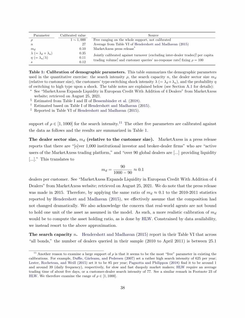
Parameter Calibrated value Sourceρ 1 ∼ 1, 000 Free ranging on the whole support, not calibratedn 27 Average from Table VI of Hendershott and Madhavan (2015)

md 0.10 MarketAxess press release*

λ (= λd + λu) 0.35Jointly calibrated against turnover (excluding inter-dealer trades)§, per capita

trading volume†, and customer queries’ no-response rate‡, fixing ρ = 100η (= λu/λ) 0.11s 0.12

Table 1: Calibration of demographic parameters. This table summarizes the demographic parametersused in the quantitative exercise: the search intensity ρ, the search capacity n, the dealer sector size md

(relative to customer size), the customers’ type-switching shock intensity λ (= λd+λu), and the probability ηof switching to high type upon a shock. The table notes are explained below (see Section A.1 for details):∗ See “MarketAxess Expands Liquidity in European Credit With Addition of 4 Dealers” from MarketAxess

website; retrieved on August 25, 2021.§ Estimated from Table I and II of Bessembinder et al. (2018).† Estimated based on Table I of Hendershott and Madhavan (2015).‡ Reported in Table VI of Hendershott and Madhavan (2015).

support of ρ ∈ [1, 1000] for the search intensity.11 The other five parameters are calibrated against

the data as follows and the results are summarized in Table 1.

The dealer sector size, md (relative to the customer size). MarketAxess in a press release

reports that there are “[o]ver 1,000 institutional investor and broker-dealer firms” who are “active

users of the MarketAxess trading platform,” and “over 90 global dealers are [...] providing liquidity

[...].” This translates to

md =90

1000− 90≈ 0.1

dealers per customer. See “MarketAxess Expands Liquidity in European Credit With Addition of 4

Dealers” from MarketAxess website; retrieved on August 25, 2021. We do note that the press release

was made in 2015. Therefore, by applying the same ratio of md ≈ 0.1 to the 2010-2011 statistics

reported by Hendershott and Madhavan (2015), we effectively assume that the composition had

not changed dramatically. We also acknowledge the concern that real-world agents are not bound

to hold one unit of the asset as assumed in the model. As such, a more realistic calibration of md

would be to compute the asset holding ratio, as is done by HLW. Constrained by data availability,

we instead resort to the above approximation.

The search capacity n. Hendershott and Madhavan (2015) report in their Table VI that across

“all bonds,” the number of dealers queried in their sample (2010 to April 2011) is between 25.1

11 Another reason to examine a large support of ρ is that it seems to be the most “free” parameter in existing thecalibrations. For example, Duffie, Garleanu, and Pedersen (2007) set a rather high search intensity of 625 per year;Lester, Rocheteau, and Weill (2015) set it to be 85 per year; Pagnotta and Philippon (2018) find it to be around 1and around 39 (daily frequency), respectively, for slow and fast duopoly market makers; HLW require an averagetrading time of about five days, or a customer-dealer search intensity of 77. See a similar remark in Footnote 23 ofHLW. We therefore examine the range of ρ ∈ [1, 1000].

38

to 27.7, depending on the trade size. A similar number is reported by O’Hara and Zhou (2021)

(“[t]he number of dealers contacted this way [...] is typically around 30,” p. 370), whose data cover

a much longer horizon from 2010 to 2017. To be precise, we take

n = 27,

closest to the 27.2 reported for “odd” size trades by Hendershott and Madhavan (2015), because

Figure 2 of O’Hara and Zhou (2021) shows that this size category constitutes the lion’s share of all

electronic trading volume.

The asset supply s, the type-switching shock intensity λ, and the probability of be-

coming high type η. These three parameters are jointly solved from a three-equation system

described below. First, Table II of Bessembinder et al. (2018) reports a turnover ratio (trading

volume relative to amount outstanding) of 0.78 for all corporate bonds in 2010. Depending on the

definition of dealers, about 71%-76% of the total trading volume is customer-based (as opposed

to inter-dealer trading), according to their Table I. We take that roughly three quarters of the

turnover ratio above is contributed by customer trading. We assume that these ratios apply to

RFQ trading, equating the model implied turnover ratio with the above numbers:

2t

s=

1

s(ρmhnνhn + ρmloνlo) = 0.78× 3

4= 58.5%. (A.1)

Recall from Equation (8) that t = ρmhnνhn = ρmloνlo is the trading volume from customer-buyers

and sellers, respectively.

Second, Table I of Hendershott and Madhavan (2015) reports that there were in total 467,614

electronic trades across 5,528 bonds in their sample of 113 years (2010 to April 2011). Per our earlier

estimate (see the calibration of md above), there were about 900 (= 1000 × (1 − 10%)) customer

institutions. Therefore, the trading intensity (per customer, per year) for an average bond is

2t

mc=

2t

1=

467, 614/435, 528× 900

≈ 0.0705. (A.2)

Third, Table VI of Hendershott and Madhavan (2015) reports the “no response” rate of the

customers’ queries. In particular, across all bonds, 8.6% of the queries of “odd size” trades had

no responses. (We focus on “odd size” trades, again, because most of the electronic trades are in

this size category, as shown in Figure 2 of O’Hara and Zhou, 2021.) In the model, a searching

customer’s query sees no reply only if all n contacts are unfortunately directed to the “wrong”

type of dealers. For example, an hn-buyer will find no response from the dealers with probability

1− νhn = (1− πdo)n = πndn, where we adopt the most parsimonious form of the matching rate π(·)

and obtain πdn = mdn/md.12 Since every instance there are ρmhn queries from hn-buyers and ρmlo

12 More elaborate parametrization for π(·), e.g., like Equation (1), will require calibration of additional parameters,like the inventory transparency ψ.

39

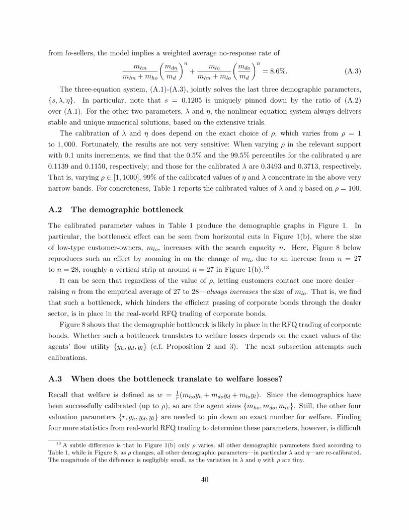
from lo-sellers, the model implies a weighted average no-response rate of

mhn

mhn +mho

(mdn

md

)n+

mlo

mhn +mlo

(mdo

md

)n= 8.6%. (A.3)

The three-equation system, (A.1)-(A.3), jointly solves the last three demographic parameters,

{s, λ, η}. In particular, note that s = 0.1205 is uniquely pinned down by the ratio of (A.2)

over (A.1). For the other two parameters, λ and η, the nonlinear equation system always delivers

stable and unique numerical solutions, based on the extensive trials.

The calibration of λ and η does depend on the exact choice of ρ, which varies from ρ = 1

to 1, 000. Fortunately, the results are not very sensitive: When varying ρ in the relevant support

with 0.1 units increments, we find that the 0.5% and the 99.5% percentiles for the calibrated η are

0.1139 and 0.1150, respectively; and those for the calibrated λ are 0.3493 and 0.3713, respectively.

That is, varying ρ ∈ [1, 1000], 99% of the calibrated values of η and λ concentrate in the above very

narrow bands. For concreteness, Table 1 reports the calibrated values of λ and η based on ρ = 100.

A.2 The demographic bottleneck

The calibrated parameter values in Table 1 produce the demographic graphs in Figure 1. In

particular, the bottleneck effect can be seen from horizontal cuts in Figure 1(b), where the size

of low-type customer-owners, mlo, increases with the search capacity n. Here, Figure 8 below

reproduces such an effect by zooming in on the change of mlo due to an increase from n = 27

to n = 28, roughly a vertical strip at around n = 27 in Figure 1(b).13

It can be seen that regardless of the value of ρ, letting customers contact one more dealer—

raising n from the empirical average of 27 to 28—always increases the size of mlo. That is, we find

that such a bottleneck, which hinders the efficient passing of corporate bonds through the dealer

sector, is in place in the real-world RFQ trading of corporate bonds.

Figure 8 shows that the demographic bottleneck is likely in place in the RFQ trading of corporate

bonds. Whether such a bottleneck translates to welfare losses depends on the exact values of the

agents’ flow utility {yh, yd, yl} (c.f. Proposition 2 and 3). The next subsection attempts such

calibrations.

A.3 When does the bottleneck translate to welfare losses?

Recall that welfare is defined as w = 1r (mhoyh +mdoyd +mloyl). Since the demographics have

been successfully calibrated (up to ρ), so are the agent sizes {mho,mdo,mlo}. Still, the other four

valuation parameters {r, yh, yd, yl} are needed to pin down an exact number for welfare. Finding

four more statistics from real-world RFQ trading to determine these parameters, however, is difficult

13 A subtle difference is that in Figure 1(b) only ρ varies, all other demographic parameters fixed according toTable 1, while in Figure 8, as ρ changes, all other demographic parameters—in particular λ and η—are re-calibrated.The magnitude of the difference is negligibly small, as the variation in λ and η with ρ are tiny.

40

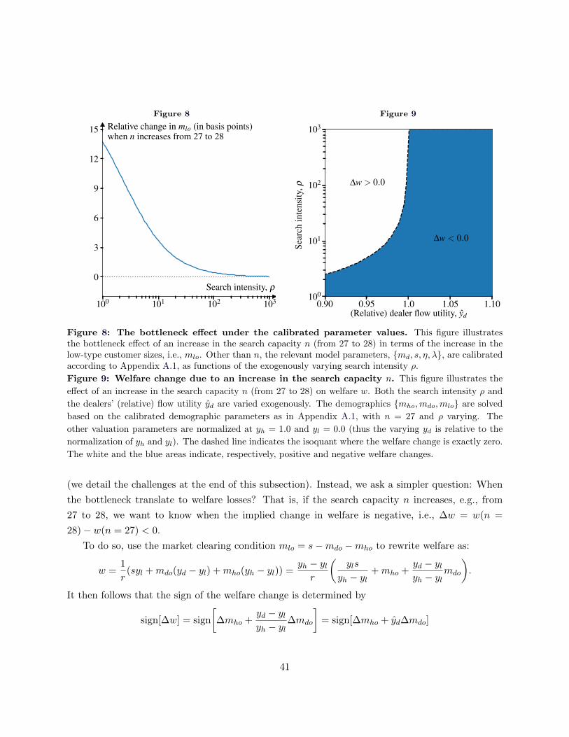
Figure 8

100 101 102 103

0

3

6

9

12

15 Relative change in mlo (in basis points)when n increases from 27 to 28

Search intensity, ρ

Figure 9

0.90 0.95 1.0 1.05 1.10(Relative) dealer flow utility, yd

100

101

102

103

Sear

chin

tens

ity,ρ ∆w > 0.0

∆w < 0.0

Figure 8: The bottleneck effect under the calibrated parameter values. This figure illustratesthe bottleneck effect of an increase in the search capacity n (from 27 to 28) in terms of the increase in thelow-type customer sizes, i.e., mlo. Other than n, the relevant model parameters, {md, s, η, λ}, are calibratedaccording to Appendix A.1, as functions of the exogenously varying search intensity ρ.

Figure 9: Welfare change due to an increase in the search capacity n. This figure illustrates the

effect of an increase in the search capacity n (from 27 to 28) on welfare w. Both the search intensity ρ and

the dealers’ (relative) flow utility yd are varied exogenously. The demographics {mho,mdo,mlo} are solved

based on the calibrated demographic parameters as in Appendix A.1, with n = 27 and ρ varying. The

other valuation parameters are normalized at yh = 1.0 and yl = 0.0 (thus the varying yd is relative to the

normalization of yh and yl). The dashed line indicates the isoquant where the welfare change is exactly zero.

The white and the blue areas indicate, respectively, positive and negative welfare changes.

(we detail the challenges at the end of this subsection). Instead, we ask a simpler question: When

the bottleneck translate to welfare losses? That is, if the search capacity n increases, e.g., from

27 to 28, we want to know when the implied change in welfare is negative, i.e., ∆w = w(n =

28)− w(n = 27) < 0.

To do so, use the market clearing condition mlo = s−mdo −mho to rewrite welfare as:

w =1

r(syl +mdo(yd − yl) +mho(yh − yl)) =

yh − ylr

(yls

yh − yl+mho +

yd − ylyh − yl

mdo

).

It then follows that the sign of the welfare change is determined by

sign[∆w] = sign

[∆mho +

yd − ylyh − yl

∆mdo

]= sign[∆mho + yd∆mdo]

41

where the difference notation ∆ is understood as the difference between n = 28 and n = 27, under

the demographic parameters calibrated in Section A.1. That is, instead of calibrating all four

valuation parameters, it suffices to know the relative dealer valuation yd :=yd−ylyh−yl .

That is, we now have two “free” parameters, the search intensity ρ and the dealer relative flow

utility yd. Figure 9 shows the result. It can be seen that the relative welfare change is negative

whenever yd is sufficiently high, for all levels of ρ. In particular, yd ≈ 1 or, equivalently, yd ≈ yh

suffices for the bottleneck to translate to welfare losses.14

To conclude, this quantitative exercise has carried the theoretical bottleneck prediction to the

real-world RFQ trading of corporate bonds, finding two results. First, for a wide, realistic range of

search intensity ρ, the bottleneck always exists (Figure 8). Second, the bottleneck indeed translates

to welfare losses, when dealers and customers value the bonds’ coupons similarly (i.e., yd ≈ yh;

Figure 9). Taken together, we find that restricting the search capacity n may have positive welfare

impacts.

Difficulty in identifying the valuation parameters

Under additional assumptions, a number of studies have calibrated the exact welfare values, like

HLW, Pagnotta and Philippon (2018), Lester, Rocheteau, and Weill (2015). Doing so requires the

identification of four other model parameters, {r, yh, yd, yl}, and below we detail the challenges of

doing so in our setting. To begin with, the literature typically normalizes r and one of the flow

utility ys. For example, HLW set r = yh = 0.05. This leaves yl and yd to be pinned down by

matching with statistics about the asset price, like trading costs and yield spreads.

While welfare per se only depends on the above four parameters {r, yh, yd, yl}, calibrating the

model to real-world price statistics, however, also requires knowledge about additional parame-

ters in our model, in particular, the exit rates {fc, fd} and the trading gain splits γlo and γhn,

which all enter the agents’ value functions and, hence, also the prices (Section 2.2 and 2.4). 15

Thus, after normalizing r and yh (as in HLW), we are still left with six valuation parameters,

{yl, yd, fc, fd, γlo, γhn}, to calibrate. To the best of our knowledge, however, only two statistics

about asset prices, applicable to our model, have been used in the literature for such calibration:

the trading cost (bid-ask spread or dealer markups) and the yield (or yield / dividend spread, as

in, e.g., Pagnotta and Philippon, 2018 and HLW).

The literature reduces the number of the unidentified valuation parameters by making reason-

14 Absent of an exact calibration, we note that a relatively high yd is economically plausible. For example,one can interpret the consumption good produced by the asset as the coupons paid out by the bond. Absentany shocks, naturally, both customers and dealers should value such dollar payments exactly the same, suggestingyd = yh = “common value”. When negative shocks, e.g., liquidity needs, strike, the valuation for such coupon flowswill drop, resulting in yl < yd = yh.

15 Note that the customers’ bargaining power q (above and beyond the dealers’ competition) enters the tradinggain splits {γhn, γlo} through the specific form of price determination assumed in Section 1. Calibrating γlo and γhnis therefore more general and flexible, as no particular assumption on price formation is imposed.

42

able approximations. For example, most of the papers have fc = fd = 0, which would be reasonable

in our model if the exits of both customers and dealers are sufficiently rare. Further, in the con-

text of BB, DGP and in HLW, assume symmetry between customer buys and sells and argue for

γlo = γhn = γ (the same Nash bargaining across all customer-dealer meetings). Assuming so in the

context of SMS, however, is less realistic, as customers on the short and long side of the market

face different competition among the dealers and so should expect to extract different fractions of

trading gains. Thus, we have at least 4 parameters {yl, yd, γlo, γhn}, facing only two price statistics.

In summary, we lack the moment conditions needed to pin down the valuation parameters and

to quantify welfare implications of the bottleneck. Instead, we let the relative utility flow yd to

be “free” parameter. This allows this subsection to comprehensively examine when the bottleneck

found in Section A.1 translates to welfare losses, as opposed to relying on a single point estimation

of welfare.

B Collection of proofs

The proofs of all the lemmas are deferred to Supplementary Appendix S1, where we also provide

additional useful results to facilitate equilibrium characterization.

Proposition 1

Proof. Note that the trading gain is ∆ = Rhn−Rlo = (Vho−Vhn)−(Vlo−Vln), a linear combination

of the four unknown value functions. The four equations (10)-(13), therefore, is a linear equation

system that uniquely pins down the four unknowns.

It only remains to prove that the trading gains are strictly positive when yd≤ yd ≤ yd.

Difference Equation (10) and (13) to get 0 = yh − (r + fc)Rh − ζhn∆hd − λd · (Rh −Rl). Similarly,

difference Equation (12) and (11) to get 0 = yl − (r + fc)Rl + ζlo∆dl + λu · (Rh − Rl). Finally,

difference the two dealers’ HJB equations, (14) and (15), to get yd− (r+ fd)Rd+ ζdo∆hd− ζdn∆dl.

Note that ∆hd = Rh−Rd and ∆dl = Rd−Rl. Therefore, taking the ζs as given, the above form a 3-

equation-3-unknown linear system, from which the reservation values {Rh, Rd, Rl} can be uniquely

solved. The resulting expressions are complicated and omitted here, but it is straightforward to

verify that Rh − Rd (resp., Rd − Rl) is monotone decreasing (resp., increasing) in yd. (Note that

the trading gain intensities ζs are independent of yd). Therefore, one can find the upper and the

lower thresholds by solving y′d explicitly from Rh = Rd and y

′

dfrom Rd = Rl:

y′d :=

ξyh(ζlo + λu + r + fc) + ξλdyl + ζdn(yh − yl)

ζlo + λd + λu + rc, and

y′

d:=

ξyl(ζhn + λd + r + fc) + ξλuyh + ζdo(yl − yh)

ζhn + λd + λu + r + fc,

where ξ is defined in the proposition. The above thresholds are still endogenous of the ζs. To

43

obtain the thresholds composed of exogenous parameters, note that

y′d ≥ yhξ −

(yh − yl)ξλdλd + λu + r + fc

=: yd and y′

d≤ ylξ +

(yh − yl)ξλuλd + λu + r + fc

=: yd.

Clearly, yd > yd. As such, y

d≤ yd ≤ yd is sufficient to ensure Rl < Rd < Rh. □

Proposition 2

Proof. The effects of ρ and n are proved separately below. For concreteness, assume that the asset

is in excess supply. (The case of excess demand is symmetric and omitted.)

A higher search intensity ρ: The trading volume can be written as t = ρmhnνhn (Equation 8).

Equation (S3) gives another link between t and mhn. Combining the two gives

t =(1 +mdo − s)λuρ

(λd + λu)ν−1hn + ρ

, (B.1)

which is increasing in ρ and in mdo (note that νhn is also increasing in mdo). Lemma S1.2 has

shown that a higher ρ increases mdo (given excess supply). Therefore, the volume increases with ρ.

It is then also clear from (S2) that mlo decreases. Finally, mhn = νloνhn

mlo by (8). The ratioνloνhn

=1−πn

do1−(1−πdo)n . Simply computing the derivative with respect to πdo can show that the ratio

decreases with πdo. That is, a higher ρ, increasing mdo and πdo, results in a lower mhn as well.

A larger search capacity n: Lemma S1.2 has shown that a larger n also increases mdo (given

excess supply). Note that since νhn = 1 − (1 − π(mdo/md))n, ∂νhn

∂mdo> 0 and ∂νhn

∂n > 0. From the

same expression of t above, therefore, n also increases trading volume. Again, from Equation (S2),

it is clear that mlo, the long-side, then decreases with n.

The effect on mhn = νloνhn

mlo, the short-side, is more complicated, because now n also affects the

ratio νloνhn

. To prove the statement, instead, it is easier to turn to the following equivalent expression:

mhn(mdo, n) :=t

ρνhn=

(1 +mdo − s)λuλd + λu + ρ(1− (1− π(mdo/md))

n), (B.2)

where the second equality follows Equation (S3). It is straightforward to find that limρ→0∂mhn∂n =

0; and limρ→0∂mhn∂mdo

= λuλd+λu

> 0. Directly computation using (S23) implies limρ→0dmdodn > 0.

Therefore, limn→∞dmhndn = limn→∞

(∂mhn∂n + ∂mhn

∂mdo

dmdodn

)> 0. □

Proposition 3

Proof. The proof considers the changes in ρ and in n separately. Only the case of excess supply,

i.e., s > η +md/2, is analyzed (and the case of excess demand is analogous and is omitted).

When ρ increases: Recall welfare is w = (yhmho + ydmdo + ylmlo)/r. By market clearing (2),

substitute mlo = s −mho −mdo in the above welfare expression to get w = (yls + (yh − yl)mho +

44

(yd − yl)mdo)/r. By Lemma S1.2, mdo increases with ρ. By Proposition 2, mhn and mlo decrease

with ρ. That is, mho = η − mhn increases with ρ. Note that yd ∈ [yd, yd] is assumed to ensure

positive trading gains (Proposition 1) and we also have that yl < yd< yd < yh. It then follows

that yd ∈ (yl, yh). Therefore, welfare is increasing with ρ.

When n increases: Welfare can be written as w = (yls+ (yd − yl)mdo + (yh − yl)(η −mhn))/r.

The effect of n goes through mdo and mhn, which are linked through the trading volume definition

of t = ρmhnνhn. In the proof of Proposition 2, it has been shown that mhn can be written as a

function of mdo and n; see Equation (B.2). Applying the chain rule yields

dmhn

dn=∂mhn

∂n+∂mhn

∂mdo

dmdo

dn. (B.3)

Combining the above, one can see that

dw

dn=

1

r

((yd − yl)

dmdo

dn− (yh − yl)

dmhn

dn

)=

1

r

(((yd − yl)− (yh − yl)

∂mhn

∂mdo

)dmdo

dn− (yh − yl)

∂mhn

∂n

).

Therefore, three derivatives of ∂mhn∂n , ∂mhn

∂mdo, and dmdo

dn need to be evaluated under ρ → 0 and

under ρ→ ∞.

Consider first the case of ρ→ 0. Directly computing the first partial derivative yields

∂mhn

∂n=λu(1 +mdo − s)

(1− mdo

md

)nρ log

(1− mdo

md

)(λd + λu + ρ

(1−

(1− mdo

md

)n))2 , (B.4)

from which it follows that limρ→0∂mhn∂n = 0. Also, limρ→0

∂mhn∂mdo

= λuλd+λu

= η. Hence, limρ→0dmhndn =

η limρ→0dmdodn . Therefore, limρ→0

dwdn = 1

r

((yd − yl) limρ→0

dmdodn − (yh − yl)η limρ→0

dmdodn

)= 1

r (yd−y) limρ→0

dmdodn /r, where y := ηyh + (1 − η)yl. Note that limρ→0

dmdodn > 0 because (i) from (S18),

limρ→0mdo ∈ (0,md); and (ii) given the excess supply, mdo increases in n (Lemma S1.2). Therefore,

sign[limρ→0

dwdn

]= sign[yd − y], proving the statement.

Next, consider the case of ρ→ ∞. Note that dmdodn > 0 (Lemma S1.2). Then signing dw

dn in

this case is equivalent to

sign

[limρ→∞

dw

dn

]= sign

[yd − ylyh − yl

− limρ→∞

(dmhndndmdodn

)].

Next, we use (B.4) to calculate ∂mhn∂n ≤ 0. Equation (B.4) then implies that limρ→∞

dmhndn

dmdodn

≤

limρ→∞∂mhn∂mdo

= 0. This implies that limρ→∞dwdn > 0. □

45

Proposition 4

Proof. Similar to the proof of Proposition 3 one can see that

dw

dψ=

1

r

((yd − yl)

dmdo

dψ− (yh − yl)

dmhn

dψ

)=

1

r

(((yd − yl)− (yh − yl)

∂mhn

∂mdo

)dmdo

dψ− (yh − yl)

∂mhn

∂ψ

).

Therefore, three derivatives of ∂mhn∂ψ , ∂mhn

∂mdo, and dmdo

dψ need to be evaluated under ρ → 0 and

under ρ→ ∞.

Consider first the case of ρ → 0. Directly computing the first partial derivative yields we

get that limρ→0∂mhn∂ψ = 0. Also, limρ→0

∂mhn∂mdo

= λuλd+λu

= η. Hence, limρ→0dmhndψ = η limρ→0

dmdodψ .

Therefore, limρ→0dwdψ = 1

r

((yd − yl) limρ→0

dmdodψ − (yh − yl)η limρ→0

dmdodψ

)= 1

r (yd−y) limρ→0dmdodψ /r,

where y := ηyh+ (1− η)yl. Note that limρ→0dmdodψ > 0. Therefore, sign

[limρ→0

dwdψ

]= sign[yd − y],

proving the statement.

Next, consider the case of ρ → ∞. ] Note that dmdodψ > 0 (Lemma S1.3). Then signing dw

dψ

in this case is equivalent to

sign

[limρ→∞

dw

dψ

]= sign

[yd − ylyh − yl

− limρ→∞

(dmhndψ

dmdodψ

)].

Next, it follows from from (B.2) that ∂mhn∂n ≤ 0. Implicit function theorem applied to (B.2) then

implies that limρ→∞

(dmhndψ /dmdo

dψ

)≤ limρ→∞

∂mhn∂mdo

= 0. This implies that limρ→∞dwdψ > 0. □

Proposition 5

Proof. Proposition S4 shows how the trading gains are split between one searching customer and n

potential counterparty dealers. Recall that with probability q, the customer is able to capture the

full trading gain. Therefore, conditional on finding at least one dealer of her matching type, an

hn-buyer expects a profit of q∆hd + (1 − q)(Rh − (Rd + A∆hd)) = (q + (1 − q)(1 − A))∆hd, while

an lo-seller expects q∆dl + (1− q)((Rd − A∆hd)− Rd) = (q + (1− q)(1− B))∆dl. Substituting in

A and B gives the stated γ(·) expression. □

Proposition 6

Proposition 6 only characterizes the equilibrium for the case of n = nSMS > 2, which guarantees

that π∗ ≤ 12 by Lemma S1.4. Before proceeding to the proof, we first add the case of n = 2:

Proposition (Equilibrium technology choices when n = 2). If π∗ ≤ 12 , Proposition 6 holds.

If π∗ > 1/2, a unique stationary equilibrium exists depending on the asset supply s: There exist

thresholds 0 < shn,0 < shn,1 ≤ slo,1 < slo,0 < 1 +md so that

46

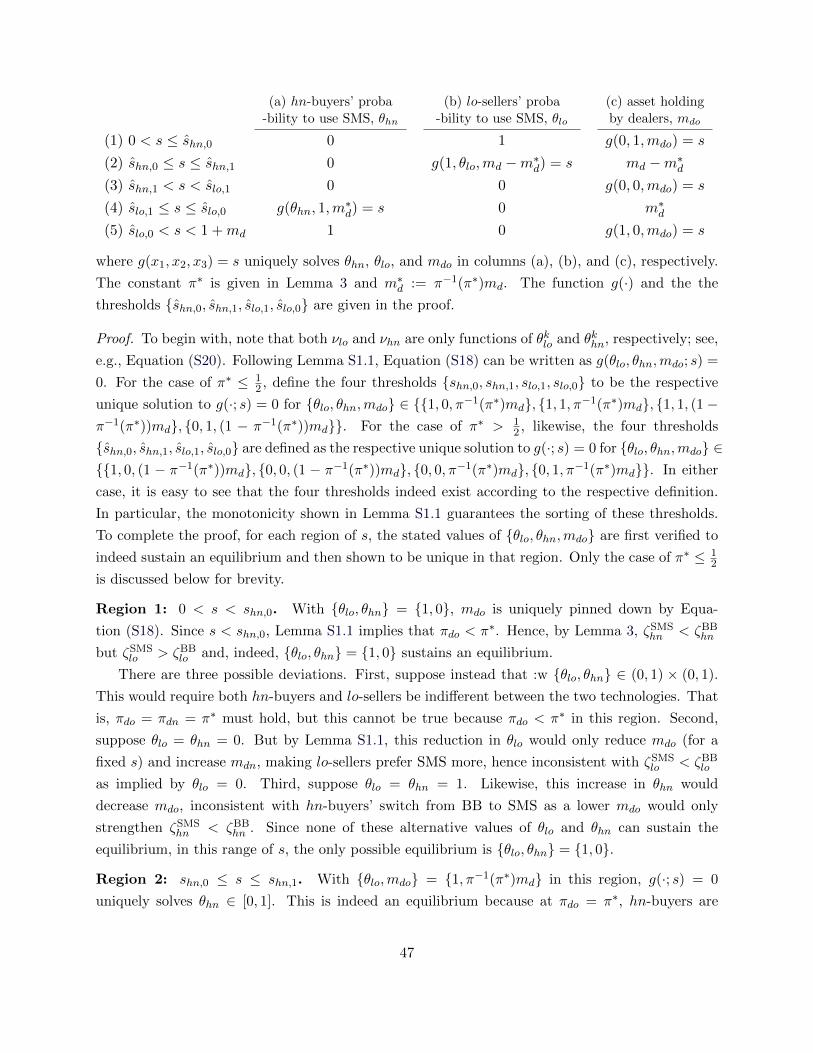
(a) hn-buyers’ proba-bility to use SMS, θhn

(b) lo-sellers’ proba-bility to use SMS, θlo

(c) asset holdingby dealers, mdo

(1) 0 < s ≤ shn,0 0 1 g(0, 1,mdo) = s

(2) shn,0 ≤ s ≤ shn,1 0 g(1, θlo,md −m∗d) = s md −m∗

d

(3) shn,1 < s < slo,1 0 0 g(0, 0,mdo) = s

(4) slo,1 ≤ s ≤ slo,0 g(θhn, 1,m∗d) = s 0 m∗

d

(5) slo,0 < s < 1 +md 1 0 g(1, 0,mdo) = s

where g(x1, x2, x3) = s uniquely solves θhn, θlo, and mdo in columns (a), (b), and (c), respectively.

The constant π∗ is given in Lemma 3 and m∗d := π−1(π∗)md. The function g(·) and the the

thresholds {shn,0, shn,1, slo,1, slo,0} are given in the proof.

Proof. To begin with, note that both νlo and νhn are only functions of θklo and θkhn, respectively; see,

e.g., Equation (S20). Following Lemma S1.1, Equation (S18) can be written as g(θlo, θhn,mdo; s) =

0. For the case of π∗ ≤ 12 , define the four thresholds {shn,0, shn,1, slo,1, slo,0} to be the respective

unique solution to g(·; s) = 0 for {θlo, θhn,mdo} ∈ {{1, 0, π−1(π∗)md}, {1, 1, π−1(π∗)md}, {1, 1, (1−π−1(π∗))md}, {0, 1, (1 − π−1(π∗))md}}. For the case of π∗ > 1

2 , likewise, the four thresholds

{shn,0, shn,1, slo,1, slo,0} are defined as the respective unique solution to g(·; s) = 0 for {θlo, θhn,mdo} ∈{{1, 0, (1 − π−1(π∗))md}, {0, 0, (1 − π−1(π∗))md}, {0, 0, π−1(π∗)md}, {0, 1, π−1(π∗)md}}. In either

case, it is easy to see that the four thresholds indeed exist according to the respective definition.

In particular, the monotonicity shown in Lemma S1.1 guarantees the sorting of these thresholds.

To complete the proof, for each region of s, the stated values of {θlo, θhn,mdo} are first verified to

indeed sustain an equilibrium and then shown to be unique in that region. Only the case of π∗ ≤ 12

is discussed below for brevity.

Region 1: 0 < s < shn,0. With {θlo, θhn} = {1, 0}, mdo is uniquely pinned down by Equa-

tion (S18). Since s < shn,0, Lemma S1.1 implies that πdo < π∗. Hence, by Lemma 3, ζSMShn < ζBB

hn

but ζSMSlo > ζBB

lo and, indeed, {θlo, θhn} = {1, 0} sustains an equilibrium.

There are three possible deviations. First, suppose instead that :w {θlo, θhn} ∈ (0, 1) × (0, 1).

This would require both hn-buyers and lo-sellers be indifferent between the two technologies. That

is, πdo = πdn = π∗ must hold, but this cannot be true because πdo < π∗ in this region. Second,

suppose θlo = θhn = 0. But by Lemma S1.1, this reduction in θlo would only reduce mdo (for a

fixed s) and increase mdn, making lo-sellers prefer SMS more, hence inconsistent with ζSMSlo < ζBB

lo

as implied by θlo = 0. Third, suppose θlo = θhn = 1. Likewise, this increase in θhn would

decrease mdo, inconsistent with hn-buyers’ switch from BB to SMS as a lower mdo would only

strengthen ζSMShn < ζBB

hn . Since none of these alternative values of θlo and θhn can sustain the

equilibrium, in this range of s, the only possible equilibrium is {θlo, θhn} = {1, 0}.

Region 2: shn,0 ≤ s ≤ shn,1. With {θlo,mdo} = {1, π−1(π∗)md} in this region, g(·; s) = 0

uniquely solves θhn ∈ [0, 1]. This is indeed an equilibrium because at πdo = π∗, hn-buyers are

47

indifferent between SMS and BB and, hence, any θhn ∈ [0, 1] is admissible. On the other hand,

πdo = π∗ < 12 implies that mdo < md/2 (recall that π(x) ≥ x by assumption) and so mdn > md/2.

It then follows that πdn > mdn/md >12 > π∗ (because π∗ < 1/2). Therefore, ζSMS

lo > ζBBlo by

Lemma 3 and θlo = 1 is sustained.

To rule out other equilibria, consider alternative values. Suppose πdo > π∗, implying θhn = 1.

Recall that s = shn,1 is the unique solution to g(·; s) = 0 when θlo = θhn = 1 and mdo = π−1(π∗)md.

The monotonicity in Lemma S1.1 would then require s > shn,1, out of this region. Suppose instead

πdo < π∗, implying θhn = 0. Then, similarly, the monotonicity in Lemma S1.1 would require

s < shn,0, again out of this region. Finally, suppose πdo = π∗ but θlo < 1. Then πdo = π∗ < 12

implies that mdo < md/2 and so mdn > md/2. It then follows that πdn > mdn/md >12 > π∗,

implying θlo = 1, a contradiction.

Region 3: shn,1 < s < slo,1. When θlo = θhn = 1, shn,1 < s < slo,1 ensures that mdo as solved

from g(·; s) = 0 satisfies π−1(π∗)md < mdo < π−1(1 − π∗)md; and, hence, πdn > π∗. That is,

ζSMS > ζBB for both hn and lo, which indeed guarantee that θlo = θhn = 1 as an equilibrium.

Again, consider other values for {θlo, θhn}. First, {θlo, θhn} ∈ (0, 1)2 cannot be an equilibrium for

the same reason as explained in Region 1. Second, suppose {θlo, θhn} = {1, 0}. By Lemma S1.1, this

reduction in θhn would result in an increase inmdo, but such an increase would only make SMS more

attractive for hn-buyers, contradicting the reduction of θhn. Third, suppose {θlo, θhn} = {0, 1}.Then similarly by Lemma S1.1, this reduction in θlo would result in a decrease in mdo or an increase

in mdn, but such an increase would only make SMS more attractive for lo-sellers, contradicting the

reduction of θlo.

Region 4: slo,1 ≤ s ≤ slo,0. This region mirrors Region 2 and the proof is omitted for brevity.

Region 5: slo,0 < s < 1 + md. This region mirrors Region 1 and the proof is omitted for

brevity. □

Proposition 7

Proof. We consider the case of s > shn,1 and prove that the ratio defined in (24) weakly decreases

in s. The volume share ratio, V S, in this region can be written as

ρSMSmSMSlo νSMS

lo + ρSMSmSMShn νSMS

hn(ρSMSmSMS

lo νSMSlo + ρSMSmSMS

hn νSMShn

)+(ρBBmBB

lo νBBlo + ρBBmBB

hn νBBhn

) =1

2+

1

2

mSMSlo νSMS

lo

mSMShn νSMS

hn

.

This is because in the considered region, θhn = 1. Then the dealer stationarity (S8) reduces to

ρSMSmSMSlo νSMS

lo + ρBBmBBlo ν

BBlo = ρSMSmSMS

hn νSMShn . (B.5)

We consider three cases next:

• s < slo,1. In this case, θlo = 1, which means that the dealer stationarity condition (S8) writes

as ρSMSmSMSlo νSMS

lo = ρSMSmSMShn νSMS

hn implying V S = 1.

48

• s > slo,0. In this case, θlo = 0, implying V S = 1/2.

• slo,1 ≤ s ≤ slo,0. In this case, mdo is a constant, invariant of s, and so both νBBlo and νSMSlo

are constants as well. Then signdV Sds = sign d

ds

(mSMSlo /mSMS

hn

). Using again (B.5),

mSMSlo

mSMShn

=ρSMSmSMS

lo νSMShn

ρSMSmSMSlo νSMS

lo + ρBBmBBlo ν

BBlo

=ρSMSνSMS

hn

ρSMSνSMSlo + ρBBνBB

lo

(mBB

lo

mSMSlo

)Using the stationarity conditions (S4) and (S5),

mSMSlo

mBBlo

=λu + ρBBνBB

lo

λu + ρSMSνSMSlo

θlo1− θlo

,

increasing in θlo, which is the only variable endogenous of s. Proposition 6 has shown that in

this range, θlo decreases with s. Therefore, by chain rule, signdVds < 0.

Combining the three cases completes the proof for the claims regarding s. To prove the claims re-

garding λd, note that from Equation (S18), cateris paribus, the left-hand side is monotone increasing

in λd (the excess supply implies νhn > νlo; see Equation (S22)) but decreasing in s. Therefore,

increases in s are equivalent to those in λd. Hence, all results about s above also hold for λd. □

Proposition 8

Proof. Since nBB = 1 < nSMS, below the notation n, without the superscript, indicates nSMS.

Proposition S4 gives the expression of Bk for k ∈ {BB, SMS}. In particular, BBB = 1, and for

SMS, BSMS =n·(1−πdo)πn−1

do

1−(1−πdo)k. Then BSMS/BBB = BSMS. By Lemma S1.1, mdo is weakly increasing

with s and hence so does πdo, thus proving the claim. To prove the claims regarding λd, note that

from Equation (S18), cateris paribus, the left-hand side is monotone increasing in λd (the excess

supply implies νhn > νlo; see Equation S22) but decreasing in s. Hence, all results about s hold

for λd. □

Proposition 9 and 10

Proof. Welfare can be written as w = 1r (yls+ (yd − yl)mdo + (yh − yl)(η −mhn)). Consider a small

change in either θ ∈ {θhn, θlo}. We then have

sign

[dw

dθ

]= sign

[(yd − yl)

dmdo

dθ− (yh − yl)

dmhn

dθ

].

Moreover, following mho +mhn = η and using the expressions (S2) and (S3), we have

dmhn

dθ= −dmhn

dθ= η

dmdo

dθ− 1

λu + λd

dt

dθ. (B.6)

Combining the above two, we get

sign

[dw

dθ

]= sign

[(yd − y)

dmdo

dθ+yh − ylλu + λd

dt

dθ

], (B.7)

49

where y := ηyh + (1− η)yl. The derivative of dmdodθ can be signed by the implicit function theorem

using the results from Lemma S1.1: dmdodθlo

> 0 and dmdodθhn

< 0. To see how volume t changes with

respect to θ, recall from Equations (S2) and (S3) and use t = ρmloνlo = ρmhnνhn to get

t =λd(s−mdo)λd+λuρνlo

+ 1and t =

λu(1 +mdo − s)λd+λuρνhn

+ 1. (B.8)

Note that θhn in the first expression only affects t through mdo. Therefore, t is increasing in θlo.

Likewise, θlo affects t in the second expression only through mdo. Hence, t is also increasing in θhn.

That is, dtdθ > 0 for either θ ∈ {θlo, θhn}.

The case of sufficiently high ρ, i.e., ρ := min[ρBB, ρSMS] → ∞: Since dtdθ > 0,

sign

[limρ→∞

dw

dθ

]= sign

[(yd − y) lim

ρ→∞

(dmdo

dθ/dt

dθ

)+yh − ylλu + λd

].

Hence, one needs to find limρ→∞

(dmdodθ / dt

dθ

).

Consider first θ = θlo. Then differentiate the second expression of t in (B.8) with respect

to θ = θlo, to get(λd+λuνhn

+ ρ)

dtdθ = ρλu

dmdodθ . Hence, limρ→∞

(dmdodθ / dt

dθ

)= 1

λu. (Note that

νkhn = 1−(1−mdo/md)nk

is always nonzero, becausemdo > md/2 in the case of excess supply.) Then

sign[limρ→∞

dwdθ

]= sign

[yd−yλu

+ yh−ylλu+λd

]= sign[yd − y − (yh − yl)η] = sign[yd − yl] > 0. (Recall

that yd ∈ (y′d, y

′d) ⊂ (yl, yh) by Corollary ??).

Consider θ = θhn. Then differentiate the first expression of t in (B.8) with respect to θ = θhn.

As ρ → ∞, the limit of mdo may be binding at md, resulting in νlo → 0. If it is not binding, i.e.,

if limρ→∞mdo < md, then νklo > 0 and limρ→∞

(dmdodθ / dt

dθ

)= − 1

λd. If it is binding, i.e., mdo → md

and νlo → 0, however ρνlo has a strictly positive limit as folows from (S18). Then, one can

again derive limρ→∞

(dmdodθ / dt

dθ

)> − 1

λd. Therefore, sign

[limρ→∞

dwdθ

]> sign

[−yd−y

λd+ yh−yl

λu+λd

]=

sign[−yd + y − (yh − yl)(1− η)] = sign[yh − yd] > 0.

The case of sufficiently low ρ, i.e., ρ := max{ρBB, ρSMS} → 0: For either θ ∈ {θlo, θhn},directly calculating dt

dθ from (B.8) and taking the limit yield limρ→0dtdθ = 0. Yet, limρ→0

dmdodθ = 0,

which follows by taking the limit in the calculations of Lemma S1.1. Hence, limρ→0dmdodθlo

> 0 and

limρ→0dmdodθhn

< 0 remain. Therefore, limρ→0 sign[dwdθ

]= sign

[(yd − y) limρ→0

dmdodθ

], proving the

statement made in the proposition. □

References

Ambrose, Brent W., Nianyun (Kelly) Cai, and Jean Helwege. 2008. “Forced Selling of FallenAngels.” The Journal of Fixed Income 18 (1):72–85.

An, Yu. 2020. “Competing with Inventory in Dealership Markets.” Working paper.

50

Anand, Amber, Chotibhak Jotikasthira, and Kumar Venkataraman. 2021. “Mutual Fund TradingStyle and Bond Market Fragility.” The Review of Financial Studies 34 (6):2993–3044.

Babus, Ana and Cecilia Parlatore. 2017. “Strategic Fragmented Markets.” Working paper.

Bessembinder, Hendrik, Stacey Jacobsen, William Maxwell, and Kumar Venkataraman. 2018.“Capital Commitment and Illiquidity in Corporate Bonds.” The Journal of Finance 73 (4):1615–1661.

Bessembinder, Hendrik, William Maxwell, and Kumar Venkataraman. 2006. “Market Transparency,Liquidity Externalities, and Institutional Trading Costs in Corporate Bonds.” Journal of Finan-cial Economics 82 (2):251–288.

Bessembinder, Hendrik, Chester Spatt, and Kumar Venkataraman. 2020. “A Survey of the Mi-crostructure of Fixed-Income Markets.” Journal of Financial and Quantitative Analysis 55 (1):1–45.

Burdett, Kenneth and Kenneth L. Judd. 1983. “Equilibrium Price Dispersion.” Econometrica51 (4):955–969.

Butters, Gerard R. 1977. “Equilibrium Distributions of Sales and Advertising Prices.” The Reviewof Economic Studies 44 (3):465–491.

Chowdhry, Bhagwan and Vikram Nanda. 1991. “Multimarket Trading and Market Liquidity.”Review of Financial Studies 4 (3):483–511.

Cujean, Julien and Remy Praz. 2015. “Asymmetric Information and Inventory Concerns in Over-the-Counter Markets.” Working paper.

Duffie, Darrell, Nicolae Garleanu, and Lasse Heje Pedersen. 2005. “Over-the-Counter Markets.”Econometrica 73 (6):1815–1847.

———. 2007. “Valuation in Over-the-Counter Markets.” The Review of Financial Studies20 (6):1865–1900.

Duffie, Darrell, Lei Qiao, and Yeneng Sun. 2019. “Continuous-time Random Matching.” Workingpaper.

Duffie, Darrell and Yeneng Sun. 2007. “Existence of Independent Random Matching.” The Annalsof Applied Probability 17 (1):386–419.

———. 2012. “The exact law of large numbers for independent random matching.” Journal ofEconomic Theory 147:1105–1139.

Dugast, Jerome, Semih Uslu, and Pierre-Olivier Weill. 2019. “A Theory of Participation in OTCand Centralized Markets.” Working paper.

Edwards, Amy K., Lawrence E. Harris, and Michael S. Piwowar. 2007. “Corporate Bond MarketTransparency and Transaction Costs.” The Journal of Finance 62 (3):1421–1452.

Ellul, Andrew, Chotibhak Jotikasthria, and Christian T. Lundblad. 2011. “Regulatory pressureand fire sales in the corporate bond market.” Journal of Financial Economics 101 (3):596–620.

Glode, Vincent and Christian C. Opp. 2019. “Over-the-Counter versus Limit-Order Markets: TheRole of Traders’ Expertise.” The Review of Financial Studies Forthcoming.

Goldstein, Michael A., Edith S. Hotchkiss, and Erik R. Sirri. 2007. “Transparency and Liquidity:

51

A Controlled Experiment on Corporate Bonds.” Review of Financial Studies 20 (2):235–274.

Hau, Harald, Peter Hoffmann, Sam Langfield, and Yannick Timmer. 2017. “Discriminatory Pricingof Over-the-Counter Derivatives.” Working paper.

Hendershott, Terrence, Dan Li, Dmitry Livdan, and Norman Schurhoff. 2017. “Relationship Trad-ing in OTC Markets.” Working paper.

———. 2020. “Fake Liquidity?” Working paper.

Hendershott, Terrence and Ananth Madhavan. 2015. “Click or Call? Auction versus Search in theOver-the-Counter Market.” The Journal of Finance 70 (1):419–447.

Hugonnier, Julien, Benjamin Lester, and Pierre-Olivier Weill. 2020. “Frictional Intermediation inOver-the-Counter Markets.” The Review of Economics Studies 87 (3):1432–1469.

Jovanovic, Boyan and Albert J. Menkveld. 2021. “Equilibrium Bid-Price Dispersion.” Journal ofPolitical Economy Forthcoming.

Klemperer, Paul. 1999. “Auction theory: A guide to the literature.” Journal of Economic Surveys13 (3):227–286.

Lagos, Ricardo and Guillaume Rocheteau. 2009. “Liquidity in Asset Markets with Search Frictions.”Econometrica 77 (2):403–426.

Lagos, Ricardo, Guillaume Rocheteau, and Pierre-Olivier Weill. 2011. “Crises and Liquidity inOver-the-Counter Markets.” Journal of Economic Theory 146 (6):2169–2205.

Lee, Tommy and Chaojun Wang. 2019. “Why Trade Over-the-Counter? When Investors WantPrice Discrimination.” Working paper.

Lester, Benjamin, Guillaume Rocheteau, and Pierre-Olivier Weill. 2015. “Competing for OrderFlow in OTC Markets.” Journal of Money, Credit and Banking 47 (S2):77–126.

Liu, Ying, Sebastian Vogel, and Yuan Zhang. 2017. “Electronic Trading in OTC Markets vs.Centralized Exchange.” Working paper.

Nash, John F. 1950. “The Bargaining Problem.” Econometrica 18 (2):155–162.

O’Hara, Maureen and Xing Zhou. 2021. “The Electronic Evolution of Corporate Bond Dealers.”Journal of Financial Economics 140 (2):368–390.

Pagano, Marco. 1989. “Trading Volume and Asset Liquidity.” The Quarterly Journal of Economics104 (2):255–274.

Pagnotta, Emiliano and Thomas Philippon. 2018. “Competing on Speed.” Econometrica86 (3):1067–1115.

Riggs, Lynn, Esen Onur, David Reiffen, and Haoxiang Zhu. 2019. “Swap Trading after Dodd-Frank:Evidence from Index CDS.” Journal of Financial Economics Forthcoming.

Saar, Gideon, Jian Sun, Ron Yang, and Haoxiang Zhu. 2020. “From Market Making to Matchmak-ing: Does Bank Regulation Harm Market Liquidity?” Working paper.

Shi, Shouyong. 2019. “Sequentially Mixed Search and Equilibrium Price Dispersion.” Workingpaper.

Sun, Yeneng. 2006. “The exact law of large numbers via Fubini extension and characterization of

52

insurable risks.” Journal of Economic Theory 126:31–69.

Uslu, Semih. 2019. “Pricing and Liquidity in Decentralized Asset Markets.” Econometrica Forth-coming.

Varian, Hal R. 1980. “A Model of Sales.” American Economic Review 70 (4):651–659.

Vayanos, Dimitri and Pierre-Olivier Weill. 2008. “A Search-Based Theory of the On-the-RunPhenomenon.” The Journal of Finance 63 (3):1361–1398.

Vogel, Sebastian. 2019. “When to Introduce Electronic Trading Platforms in Over-the-CounterMarkets?” Working paper.

Wang, Chaojun. 2017. “Core-Periphery Trading Networks.” Working paper.

Weill, Pierre-Olivier. 2007. “Leaning against the Wind.” Review of Economic Studies 74:1329–1354.

Wright, Randall, Philipp Kircher, Benoıt Julien, and Veronica Guerrieri. 2020. “Directed Searchand Competitive Search: A Guided Tour.” Journal of Economic Literature Forthcoming.

Zhu, Haoxiang. 2012. “Finding a Good Price in Opaque Over-the-Counter Markets.” The Reviewof Financial Studies 25 (4):1255–1285.

53

Simultaneous Multilateral Search

Supplementary Appendix

Sergei Glebkin∗ Bart Zhou Yueshen† Ji Shen‡

This version: January 10, 2022

• Section S1 details additional useful results and completes the proofs for the main paper.

• Section S2 compares the main model in the paper with “directed search.”

• Section S3 examines the pricing by the dealers.

• Section S4 studies a model extension where each customer can choose her search intensity ρ.

• Section S5 characterizes the transition dynamics equilibrium.

• Section S6 describes an alternative price setting mechanism and shows that it is equivalent to

the one adopted in the main model.

• Section S7 collects proofs to the results in S2-S6.

There are no competing financial interests that might be perceived to influence the analysis, the

discussion, and/or the results of this article.

∗ INSEAD; glebkin@insead.edu; Boulevard de Constance, Fontainebleau 77300, France.† INSEAD; b@yueshen.me; 1 Ayer Rajah Avenue, Singapore 138676.‡ Peking University; jishen@gsm.pku.edu.cn; No. 38 Xueyuan Road, Haidian District, Beijing 100871, China.

S1 Additional results and proofs of lemmas

S1.1 Demographics with one search technology

While the system (2)-(7) has only two zero-flow conditions (Equations 6 and 7), the stationarity

of all other types of agents is also implied. Apart from the dealer stationarity (8), −(5) − (6)

gives νlomloρ−mlnλu +mhnλd = 0, ensuring that the net flow in and out of ln-bystanders is zero.

Likewise, (5)− (7) gives νhnmhnρ−mhoλd+mloλu = 0, ensuring that the net flow of ho-bystanders

is zero.

We also derive some useful expressions for the customer masses. Equations (2), (3), and (5)

together imply the stable fractions of the high-type and the low-type customers:

mho +mhn =λu

λd + λu=: η and mlo +mln =

λuλd + λu

= 1− η. (S1)

Then combining the market clearing condition (2) and the lo-seller net flow (6), we obtain

mlo = (1− η)(s−mdo)−t

λu + λd, (S2)

which intuitively says that the stationary mass of lo-sellers is a fraction (1 − η) of the residual

asset supply (s−mdo) available to customers, less a term t/(λu + λd) due to their active trading.

Combining (2) and (6) gives

mhn = η · (1 +mdo − s)− t

λu + λd. (S3)

Note that 1+mdo−s, which is the total mass of non-owner customers in this economy. That is, the

stationary mass of hn-buyers is the high-type fraction η of all non-owner customers, less the same

term due to trading. The above expressions are in fact generic in the search literature. For example,

if, as in DGP, customers find each other at intensity ρ without dealers, then Equations (S2) and (S3)

still hold with mdo = 0 and t = 2ρmhnmlo.

S1.2 Demographics with two search technologies

There are six customer population sizes: {mho,mln,mSMShn ,mBB

hn ,mSMSlo ,mBB

lo }; in addition, there

are two types of dealers, {mdo,mdn}. For notation simplicity, write

mhn = mSMShn +mBB

hn ; and mlo = mSMSlo +mBB

lo .

Then the four (aggregate) customer masses, {mho,mln,mhn,mlo}, must satisfy the conditions (2)-

(5) in Section 2.1. The other four conditions are analogous to the stationarity conditions (6)

2

and (7):

net flow of lo-sellers using SMS: − νSMSlo mSMS

lo ρSMS − λumSMSlo + θloλdmho = 0 (S4)

net flow of lo-sellers using BB: − νBBlo mBB

lo ρBB − λum

BBlo + (1− θlo)λdmho = 0 (S5)

net flow of hn-buyers using SMS: − νSMShn mSMS

hn ρSMS − λdmSMShn + θhnλumln = 0 (S6)

net flow of hn-buyers using BB: − νBBhn m

BBhn ρ

BB − λdmBBhn + (1− θhn)λumln = 0 (S7)

where νklo = 1 −(1− mdn

md

)nk

and νkhn = 1 −(1− mdo

md

)nk

are the probabilities for a customer to

find at least one counterparty dealer using technology k ∈ {BB,SMS}. Compared to Equations (6)

and (7) in Section 2.1, the key differences are (i) that every variable here is technology-dependent

and superscripted with k ∈ {BB, SMS}; and (ii) that only a fraction of θσ of the newly shocked

σ-customer use SMS, while the rest (1− θσ) use BB, where σ ∈ {hn, lo}.The conditions (2)-(5) and (S4)-(S7) exactly pin down the eight demographic variables:

Lemma S1 (Stationary demographics with technology choice). Given the customers’ tech-

nology choices {θlo, θhn} ∈ [0, 1]2, Equations (2)-(5) and (S4)-(S7) uniquely pin down the demo-

graphics {mho,mln,mSMShn ,mBB

hn ,mSMSlo ,mBB

lo } ∈ [0, 1]6 and {mdo,mdn} ∈ (0,md)2.

The resulting expressions are similar to those implied by Lemma 1. In particular, (S4) + (S5) −(S6)− (S7) + (5) gives the trading volume expression

t :=∑k

νklomkloρ

k =∑k

νkhnmkhnρ

k, (S8)

ensuring the stationarity of both dealer types. The h- and l-type customer stationarity (S1) also

holds the same, and so do the expressions for the total size of trading customers mlo =∑

kmklo

and mhn =∑

kmkhn. The stationarity of all other types of agents are also ensured: For example,

−(5) − (S4) − (S5) gives −λumln +∑

k

(νklom

kloρ

k + λdmkhn

)= 0, which ensures the stationarity of

ln-bystanders. Likewise, (5) − (S6) − (S7) gives −λdmho +∑

k

(νkhnm

khnρ

k + λumkln

)= 0, which

ensures the stationarity of ho-bystanders.

S1.3 Value functions with two search technologies

Given the technology choices {θσ}, hence also the demographics (Lemma S1), the value functions

for all six agent types can be derived analogously to those in Equations (10)-(15). For example,

the value functions of an ho-bystander and an ln-bystander must satisfy the HJB equations

yh + λd ·(max

[V SMSlo , V BB

lo

]− Vho

)− (r + fc)Vho = 0; (S9)

λu ·(max

[V SMSho , V BB

ho

]− Vln

)− (r + fc)Vln = 0. (S10)

Compared with Equations (10) and (11), the only difference is that upon a preference shock, a newly

shocked trading customer can choose which technology to use, hence the term of max[V SMSσ , V BB

σ

]3

in the above HJBs (σ ∈ {lo, hn}).The HJB equations for the trading agents are also similar to before:

HJB of lo-sellers using technology k: yl + λu · (Vho − V klo)− (r + fc)V

klo + ζklo∆

kdl = 0; (S11)

HJB of hn-buyers using technology k: λd · (Vln − V khn)− (r + fc)V

khn + ζkhn∆

khd = 0; (S12)

HJB of do-dealers: yd − (r + fd)Vdo +∑k

ζkdo∆khd = 0; (S13)

HJB of dn-dealers: − (r + fd)Vdn +∑k

ζkdn∆kdl = 0. (S14)

Compared to Equations (12)-(15), the only difference is that the trading gains {∆hd,∆dl} and the

trading gain intensities {ζlo, ζhn, ζdo, ζdn} are technology specific, superscripted with k ∈ {BB, SMS}.For completeness, we derive these expressions below.

Using technology k, an lo-seller’s reservation value is Rkl := V klo − Vln, and that for an hn-buyer

is Rkh := Vho − V khn. A dealer’s reservation value is the same Rd := Vdo − Vdn as before. Then,

depending the customer’s technology k, the trading gain between an hn-buyer and a do-seller is

∆khd := Rkh−Rd and that between a dn-buyer and an lo-seller is ∆k

dl := Rd−Rkl . By Proposition S4,

the dealers’ respective average ask and bid are:

Ak =nk mdo

md

(1− mdo

md

)nk−1

1−(1− mdo

md

)nk and Bk =nk mdn

md

(1− mdn

md

)nk−1

1−(1− mdn

md

)nk .

Thus, an hn-buyer expects ζkhn∆khd, while a do-dealer expects ζkdo∆

khd, where the respective trading

gain intensities are

ζkhn = ρkνkhn ·(qk + (1− qk)(1− Ak)

)and ζkdo =

mkhnρ

kνkhnmdo

(1− qk)Ak.

Analogously, an lo-seller expects ζklo∆kdl, while a dn-dealer expects ζdn∆

kdl, with intensities

ζklo = ρkνklo ·(qk + (1− qk)(1− Bk)

)and ζkdn =

mkhnρ

kνklomdn

(1− qk)Bk.

Finally, with the above expressions of the value functions and trading gain intensities, we can

show that the trading gain remains positive under the same condition of yd ≥ yd ≥ ydas defined

in Proposition 1. To see why, note that in equilibrium, the trading customers either have a strict

preference for one of the technology or are indifferent. Consider lo-sellers, for example. If the

preference is strict, then only one of the two HJBs in (S11) is relevant; and if indifference, then

the two HJBs reduce to the same one. The same holds for hn-buyers in their two HJBs (S12).

Likewise, the max[·] operator in Equations (S11) and (S12) can be dropped in equilibrium. Hence,

defining Vlo = maxk[{V klo}] and Vhn = maxk[{V k

hn}], the HJB equations (S9)-(S14) can be reduced

to the exactly the same set of (10)-(15) as if there is only one technology. Therefore, solving the

4

same equation system, the same result from Proposition 1 holds. Following the same argument in

the paragraph after Proposition 1, the positive trading gains also ensures that both the ho− and

ln-customers do stay out of trading—they are indeed bystanders.

S1.4 Additional lemmas

Lemma S1.1. Write the left-hand side of Equation (S18) as a function of g(θlo, θhn,mdo, s). Then

(1) ∂g∂mdo

> 0, (2) ∂g∂θlo

< 0, (3) ∂g∂θhn

> 0, and (4) ∂g∂s < 0. In particular, (5) mdo ↓ 0 when s ↓ 0 and

mdo ↑ 1 +md when s ↑ 1 +md regardless of θlo and θhn. Finally, (6)∂mdo∂θlo

> 0 > ∂mdo∂θhn

.

Lemma S1.2. When there is excess supply, both the search intensity ρ and the capacity n increase

mdo and reduce mdn, but their effects on customers’ matching rates are different: A higher ρ

increases νhn but decreases νlo, while a larger n increases both νhn and νlo.

Lemma S1.3. When there is excess supply, the transparency ψ increase mdo and reduce mdn.

Lemma S1.4. The functions zSMS(π) and zBB(π) in Lemma 3 cross at π∗ > 12 if and only if

nSMS = 2 and 2qSMSρSMS−qBBρBB

(2qSMS−1)ρSMS > 12 .

S1.5 Proof of Lemma 1 and Lemma S1

Proof. The proof considers the general case of Lemma S1 with arbitrary θhn and θlo. Lemma 1 is

then just a special case of θhn = θlo = 1. Where convenient, we will occasionally write θSMSσ =

1 − θBBσ = θσ. The idea is to first express all other unknowns as monotone functions of mdo. The

existence and the uniqueness then follow as long as the solution to mdo exists and is unique. To

begin with, add (S4) and (S5) to get

all lo-seller stationarity: − λumlo + λdmho − ρmloνlo = 0, (S15)

where mlo :=∑

kmklo is the total lo-seller mass, ρ := max

[ρSMS, ρBB

], νlo := 1

ρmlo

∑k ρ

kmkloν

klo is

the (weighted) average matching rate for an lo-seller, and mho :=∑

kmkho is the total ho-bystander

mass. Similarly, adding (S6) and (S7) yields

all hn-buyer stationarity: − λdmhn + λumln − ρmhnνhn = 0, (S16)

where mhn :=∑

kmkhn, νhn := 1

ρmhn

∑k ρ

kmkhnν

khn, and mln :=

∑km

kln. Taking {νlo, νhn} as given,

Equations (S1), (S15), and (S16) form a linear system of the four masses {mho,mln,mhn,mlo},which have the unique solution of

mho = ηλuνhn + ρνloνhn

λuνhn + λdνlo + ρνhnνlo; mln = (1− η)

λdνlo + ρνloνhnλuνhn + λdνlo + ρνhnνlo

;

mhn = (1− η)λuνlo

λuνhn + λdνlo + ρνhnνlo; mlo = η

λdνhnλuνhn + λdνlo + ρνhnνlo

. (S17)

5

Plug in the expressions of mho and mlo =∑

kmklo into the market clearing condition (2) to get

η(λu + λd)νhn + ρνloνhnλuνhn + λdνlo + ρνloνhn

+mdo − s = 0. (S18)

This is an equation with unknowns {mdo, νhn, νlo}. It remains to express νhn and νlo as (monotone)

functions of mdo.

Consider νlo for example. Note that (S4) and (S5) imply that

mklo =

λdmhoθklo

λu + ρkνklo(S19)

where θBBlo := 1− θlo and θSMS

lo := θlo. Hence, from the earlier definition,

νlo =

∑k ρ

kmkloν

klo

ρmlo=

∑k ρ

kmkloν

klo

ρ∑

kmklo

=

∑k

ρkθkloνklo

λu+ρkνklo

ρ∑

kθklo

λu+ρkνklo

, (S20)

which is monotone increasing in both νklo for k ∈ {BB,SMS}. Recall from the definition νklo :=

1 − (1− πdn)nk

that both νklo are monotone decreasing in mdo. Therefore, so is νlo. In the same

way, both νkhn are monotone increasing in mdo and so is νhn.

Now return to Equation (S18). Since both νlo and νhn can be expressed as a unique function in

mdo, (S18) is an equation of a single unknown mdo. To prove the existence of the solution, consider

the limits of the support of mdo ∈ [0,md]. As mdo ↓ 0, both νklo ↑ 1 while both νkhn ↓ 0, and as a

result, νlo ↑ 1 and νhn ↓ 0. The left-hand side of (S18), therefore, reaches −s < 0. Reversely, as

mdo ↑ md, νlo ↓ 0 and νhn ↑ 1, the left-hand side of (S18) reaches 1 +md − s > 0 (as it is assumed

that 0 < s < 1 +md). Therefore, by continuity, the solution to mdo always exists.

To prove uniqueness, examine the derivative of the left-hand side of (S18) with respect to mdo:

−ηλd(λu + λd + ρνhn)νhn

(λuνhn + λdνlo + ρνhnνlo)2∂νlo∂mdo

+ ηλd(λu + λd + ρνlo)νlo

(λuνhn + λdνlo + ρνhnνlo)2∂νhn∂mdo

+ 1 > 0, (S21)

where the inequality holds because νlo decreases, while νhn increases, in mdo. That is, the left-hand

side of (S18) is strictly monotone increasing in mdo. Hence, there exists one and only one mdo that

solves (S18). Therefore, the demographics equation system always has a unique solution. □

S1.6 Proof of Lemma 2

Proof. Calculate the difference between mhn and mlo using the expressions (S3) and (S2) to get

mhn −mlo = η +mdo − s = ηλd ·νlo − νhn

λuνhn + λdνlo + ρνhnνlo, (S22)

where the last equality follows Equation (S18). Therefore, sign[mhn−mlo] = sign[νlo−νhn]. Recallthat νlo = 1− (1− πdn)

n and νhn = 1− (1− πdo)n, from which it follows that νlo > νhn if and only

if mdn > mdo. Given that mdn +mdo = md, therefore, mhn > mlo if and only if mdo < md/2. Use

6

again mhn −mlo = η +mdo − s, which is negative if and only if s > η +mdo > η +md/2. □

S1.7 Proof of Lemma 3

Proof. Consider first the case of ρSMSqSMSnSMS < ρBBqBBnBB. The proof first establishes the

single-crossing of zSMS(π) and zBB(π) at some π∗ ∈ (0, 1). The general idea is to characterize

the shapes of zBB(π) and zSMS(π). In particular, it will be shown that zBB is linearly increasing

in π, while zSMS is sigmoid-shaped in π, starting below zBB for sufficiently small π; and the two

satisfy zBB(0) = zSMS(0) = 0 and zBB(1) < zSMS(1). Therefore, there is always one and only one

intersection point π∗ ∈ (0, 1).

Consider zBB first. With nBB = 1, zBB = qBBρBBπ, which is linearly increasing from 0 at

π = 0 to qBBρBB at π = 1. Next, consider zSMS. For notation simplicity, the superscripts

SMS on n, ρ, and q are omitted when there is no confusion. With n = nSMS > 1 , zSMS =(1− (1− π)n−1(1− π + (1− q)nπ)

)ρ, whose first-order derivative with respect to π is ∂zSMS

∂π =

−nρ(1− π)n−2(π(1− n) + q(πn− 1)), which is positive. To see why, note that the bracketed term,

π(1 − n) + q(πn − 1) is linear in π and is negative for both π = 0 and π = 1 and so it is negative

for all π. Thus, zSMS(π) is strictly monotone increasing on π ∈ (0, 1). Its second-order derivative

with respect to π is ∂2zSMS

∂π2 = (n − 1)nρ(1 − π)n−3(π − nπ + (πn − 2)q + 1), which is positive if

and only if π < 1−2qn−1−nq . Note that 1−2q

n−1−nq > 0, because ρSMSqSMSnSMS < ρBBqBBnBB implies

q = qSMS < 1/nSMS ≤ 1/2. Summarizing the above, zSMS(·) is sigmoid-shaped for π > 0: it is

monotone increasing, initially convex, but eventually concave.

Now note that in the lower end, zSMS|π↓0 = zBB|π↓0 = 0. Further, the slope of z(·) satisfies

limπ↓0dzdπ = nρq. Therefore, the assumption ρSMSqSMSnSMS < ρBBqBBnBB ensures that for π

sufficiently small, zSMS < zBB. On the upper end of π ↑ 1, zSMS → ρSMS ≥ ρBB ≥ qBBρBB, where

the first inequality follows (18) and the second follows qBB ∈ [0, 1]. That is, zSMS exceeds zBB

eventually. Therefore, there exists a unique π∗ ∈ (0, 1) at which zSMS(π∗) = zBB(π∗).

Next, it is clear that V kσ is monotone increasing in ζkσ , where k ∈ {BB, SMS} and σ ∈ {lo, hn}.

Hence, comparing the value functions is equivalent to comparing the trading gain intensities {ζkσ};i.e., the technology choice (19) is equivalent to (22). With the single-crossing property established

above, it then follows that the comparison of the {ζkσ} is equivalent to (21).

Finally, consider the case of ρSMSqSMSnSMS ≥ ρBBqBBnBB. The only change is that the slope of

zk(π) at the lower end now is higher for SMS than for BB. Thus, the only intersection possible is at

π = 0, i.e., zSMS > zBB for all π ∈ (0, 1), i.e., SMS is always preferred and, hence, θhn = θlo = 1. □

S1.8 Proof of Lemma S1.1

Proof. (1) ∂g∂mdo

has been evaluated in (S21) in the proof of Lemma S1. (2) Note that θlo affects

g(·) only through νlo, which is given by (S20). Carefully simplifying, it can be found that ∂νlo∂θlo

=

7

(νSMSlo −νBB

lo )(λu+νSMSlo )(λu+νBB

lo )

(λu+(1−θlo)νSMSlo +θloν

BBlo )2

> 0 where the inequality holds because νSMSlo > νBB

lo always holds

(with ρSMS ≥ ρBB and nSMS > nBB = 1). The partial derivative of g(·) with respect to νlo is∂g∂νlo

= − (λd+λu+νhn)λdνhn(λuνhn+(λd+νhn)νlo)2

< 0. Therefore, by chain rule, ∂g∂θlo

< 0. (3) can be proved similarly by

showing that ∂νhn∂θhn> 0 and that ∂g

∂νhn> 0. The details are omitted for brevity. (4) is straightforward

as ∂g∂s = −1. (5) By implicit function theorem, g(·) = 0 implies that mdo strictly increases in s; see

(1) and (4) above. The limit values as s ↓ 0 or s ↑ 1 can then be easily verified, regardless of θlo

and θhn. (6) directly follows the implicit function theorem by (1)-(3). □

S1.9 Proof of Lemma S1.2

Proof. The key equation is (S18) in the proof of Lemma 1. Define the left-hand side as f(mdo, ρ, n).

Recall that Equation (S21) has shown that ∂f∂mdo

> 0. In addition, simple calculus gives sign[∂f∂ρ

]=

sign[νlo − νhn]. Since excess supply is assumed, i.e., mhn < mlo, Equation (S22) gives νlo < νhn.

Hence, dmdodρ = −∂f

∂ρ/∂f∂mdo

> 0, i.e., a higher ρ increases mdo and, because mdn = md − mdo,

decreases mdn. It then also follows that a higher ρ increases νhn = 1 − (1 − πdo)n but decreases

νlo = 1− (1− πdn)n.

Consider the effect of a larger n next. In that case it is more convenient to work with an

equivalent version of (S18):

η(1 +mdo − s)

(λd + λuνlo

+ ρ

)− (1− η)(s−mdo)

(λd + λuνhn

+ ρ

)= 0. (S23)

Define the left-hand side of (S23) as g(mdo, ρ, n). Since∂g

∂mdo> 0 we have sign

[dmdodn

]= −sign

[∂g∂n

]and it remains to sign ∂g

∂n . Taking πdo and πdn as given, then sign[∂g∂n

]= sign[hh(1− πdn)− hh(1− πdo)],

where

hh(x) := (ρ(1− xn) + λd + λu)−1 log x

x−n − 1.

Further, one can show that hh(x) is decreasing in x. Then, because πdo > πdn, hh(1 − πdn) <

hh(1− πdo). It follows thatdmdodn > 0, i.e., a higher n increases mdo and, hence, decreases mdn.

Since higher n increases mdo it follows immediately that higher n increases νhn = 1−(1− πdo)n.

To see the effect of n on νlo we first prove that trading volume is increasing in n. The trading volume

can be written as t = ρmhnνhn (Equation 8). Equation (S3) gives another link between t and mhn.

Combining the two gives

t =(1 +mdo − s)λuρ

(λd + λu)ν−1hn + ρ

,

which is increasing in n both directly and through the dependence of mdo on n. Thus, trading

volume increases in n. Now, writing t = ρmloνlo and using (S2) we obtain νlo =λd+λu

λdρ(s−mdo)

t−ρ

from

which it follows that νlo increases in n. □

8

S1.10 Proof of Lemma S1.3

Proof. Consider (S23). Define the left-hand side of (S23) as g(mdo, ψ). It is straightforward to show

that sign(∂g/∂ψ) = sign[∂∂ψ log

(λd+λuνlo

+ ρ)− ∂

∂ψ log(λd+λuνhn

+ ρ)]

. Denoting x := mdo/md, and

ν(π) := 1− (1− π)n we can express νhn = ν(π(x;ψ)) and νlo = ν(π(1− x;ψ)). For x > 1/2 (which

holds in the excess supply case) one can show that ∂π(x,ψ)∂ψ < ∂π(1−x,ψ)∂ψ . Additionaly, π(x;ψ) > π(1−

x;ψ). Then, an explicit calculation of ∂∂ψ log

(λd+λuν(π(x;ψ)) + ρ

)implies that ∂

∂ψ log(

λd+λuν(π(x;ψ)) + ρ

)>

∂∂ψ log

(λd+λu

ν(π(1−x;ψ)) + ρ). It then follows that ∂g

∂ψ < 0 and by implicit function theorem dgdψ > 0. □

S1.11 Proof of Lemma S1.4

Proof. Consider first the case nSMS > 2. To establish that π∗ ≤ 12 , note that zSMS(π) is monotone

increasing in nSMS and in qSMS. Therefore, fixing zBB(π) = qBBρBBπ, the intersection π∗ must be

higher as nSMS and qSMS reduce. Likewise, fixing zSMS(π), π∗ must be higher when the product of

qBBρBB increases. Since qBB ∈ [0, 1] and ρBB ≤ ρSMS, the maximum of this product is qBBρBB ≤ρSMS. Therefore, the maximum π∗ is the solution to zSMS(π;nSMS = 3, qSMS = 0) − ρSMSπ = 0.

Solving this equation gives the unique interior solution of π∗ = 12 . For the case nSMS = 2, we plug

nSMS = 2 into zSMS(π) and solve for π∗ in (a linear equation) zBB(π) = qBBρBBπ. Doing so yields

π∗ = 2qSMSρSMS−qBBρBB

(2qSMS−1)ρSMS . □

S2 Comparison with directed search

This appendix analyzes a model of OTC trading with “directed search” (DS), where dealers con-

tinuously post quotes and, after observing them, each customer directs her search to one chosen

dealer. This is a realistic feature of corporate bonds trading, as dealers sometimes broadcast their

indicative bids and asks to customers on electronic platforms (Section III.B of Bessembinder, Spatt,

and Venkataraman, 2020). The similarity of this paper and the DS literature is that both allow

endogenous trading gain shares accruing to customers and dealers. See, e.g., Guerrieri, Shimer,

and Wright (2010), Lester, Rocheteau, and Weill (2015), Chang (2018) and, for a review, Wright

et al. (2020). The purpose is to compare the findings of DS model in this appendix with those of

SMS from Section 2. The key result is that the steady state equilibrium under DS can be proxied

by the SMS equilibrium either (i) when the dealers inventory transparency ψ is sufficiently higher;

or (ii) when the search capacity n is sufficiently large.

S2.1 A model of directed search

The model setup follows Section 1, except for the parts of “search” and “price determination,”

which are modified as follows: All dealer owners (type do) constantly post ask quotes, while all

dealer non-owners (type dn) post bid quotes. Customers observe these quotes and direct their

9

searches to chosen dealers at independent Poisson processes with the same intensity ρ. Customers

and their chosen dealers meet pairwise and once met, the pair exchanges the asset at the dealer

quoted price.

Denote by νhn the probability for a hn-do match and by νlo for a lo-dn match. Assume that

νhn = 1 if mdo > 0 and νlo = 1 if mdn > 0. (S24)

This is because at any instant, there is only an infinitesimal amount of customers searching (ρmhndt

buyers and ρmlodt sellers), which is negligible compared to the vast mass of quoting dealers (mdo

and mdn, if positive). Effectively, the assumption (S24) lets the dt-measure customers find dealers

with certainty as long as the measures of counterparties are strictly positive. In the case when some

dealer masses become zero, i.e., mdo → 0 or mdn → 0, the matching probabilities will be solved

endogenously.

We shall look for a steady-state, symmetric dealer pricing equilibrium, characterized by the

following time-invariant variables: (i) the demographics {mho,mhn,mlo,mln,mdo,mdn}; (ii) the

matching probabilities {νhn, νlo} in case the corresponding dealer mass is zero; and (iii) the sym-

metric ask and bid, pa and pb, by the do- and dn-dealers, respectively. Note that since the quotes

are symmetric, the customers randomly direct their searches to all counterparty dealers.

S2.1.1 Demographics and matching probabilities

The six demographic variables {mho,mhn,mlo,mln,mdo,mdn} and the two matching probabilities

{νhn, νlo} can be pinned down by the six equations (2)-(7), which hold as before, plus the two

conditions given in (S24):

Proposition S1 (Demographics under DS). In a steady-state, the matching probabilities sat-

isfy

νhn = min

[1,mlo

mhn

]and νlo = min

[1,mhn

mlo

], (S25)

where the ratios mlomhn

and mhnmlo

depend on the asset supply s:

sign

[mlo

mhn− 1

]= −1{0<s<η} + 1{η+md<s<1+md}. (S26)

Given the {νhn, νlo} above, the steady-state demographics exist and are the unique solution to the

linear equation system (2)-(7).

The key insight from (S25) is that the matching probabilities {νhn, νlo} only depend on the

relative sizes of hn-buyers and lo-sellers in the market. Perhaps surprisingly, the dealer sizes mdo

and mdn do not show up, as if the customers are directly searching for counterparties, skipping the

dealers. To see why, recall that (2)-(7) also imply the dealer stationarity condition (8): ρmhnνhn =

ρmloνlo, which balances the asset inflow to and the outflow from the dealers (otherwise the dealer

10

sizes will change overtime). Note that it can be equivalently interpreted as the hn-buyers are

directly matched with the lo-sellers. That is, the dealers are merely passing the asset from the

sellers to the buyers, not affecting the matching probabilities {νhn, νlo}.One might wonder why νhn and νlo can be less than one: Since there is always only a dt

amount—zero measure—of customers searching for dealers, by assumption (S24), should not the

matching probabilities always be one? It turns out that νhn < 1 and νlo < 1 precisely when the

measure of the corresponding dealers is also zero. Consider, for example, the case ofmdo = 0, which

implies that mdn = md − mdo > 0. Then, by assumption (S24), νlo = 1 and there is always an

amount of ρmloνlodt trades occurring between dn-buyers and lo-sellers. These trades then create a

“transient” fringe of do-sellers (of the same magnitude of dt) who then quote asks to the searching

hn-buyers. The dealer stationarity condition (8) above then requires:

ρmhnνhn = ρmloνlo =⇒ νhn =mloνlomhn

=mlo

mhn.

Note that it must be νhn < 1 in this case (as verified in the proof of Proposition S1); that is,

all such transient do-sellers are sought after by hn-buyers. Otherwise, some of the do-sellers will

accumulate overtime, making the dealer masses nonstationary.

S2.1.2 Value functions and prices

The value functions can be found using the same set of HJB equations (10)-(15) as in Section 2.2.

Hence, Proposition 1 continues to hold for directed search. In particular, the condition for positive

trading gains remains the same. The only differences are in the trading gain intensities, {ζσ}.We first consider the interior equilibrium where mdo ∈ (0,md). In this case, there is perfect

competition among dealers and so ζdn = ζdo = 0. To see why, consider, for example, the do-

sellers’ quote pa to the hn-buyers. Since the amount of searching hn-buyers is vanishingly small

(ρmhndt), the standard Bertrand price competition applies to the do-sellers, giving pa = Rd as

the only symmetric price in equilibrium. Similar argument implies that in this case the dn-buyers

quote pb = Rd. Summing up, the dealers quotes are given by pa = pb = Rd, and the trading gain

intensities are given by ζlo = ρνlo, ζhn = ρνhn, and ζdo = ζdn = 0.

Next, in the corner equilibrium of mdo = 0, any do-dealer exists only transiently: Whenever a

dn-dealer has bought the asset (from an lo-seller), he immediately trades again with an hn-buyer,

becoming dn-dealer again. Therefore, ∆hd = 0 in this case. This follows from Equation (14) if one

divides it by ζdo and sets ζdo = ∞ (because a do-dealer trades immediately without waiting). Then

pa = Rh = Rd. The Bertrand competition argument for md > 0 amount of dn-buyers still implies

that pb = Rd. Likewise, in the corner equilibrium of mdn = 0, we have ∆dl = 0 and pa = pb = Rd.

11

S2.2 Comparing DS with SMS

In DS, a customer can first observe all dealers’ quotes and then direct her search to a chosen dealer.

In SMS, a customer can reach only n dealers (where n is set by the platform like RFQ), not knowing

the types of the dealers, only with noisy signals of quality ψ. This appendix concludes with the

following convergence result:

Proposition S2 (Convergence of SMS to DS). The equilibrium demographics, value functions,

and prices in the SMS model converge to those in DS either (i) when ψ → 1 under the “random

matching with signal” specification with n ≥ 2; or (ii) when n→ ∞ under the general specification.

Intuitively, one should expect as the search capacity n→ ∞, the customer can almost surely find at

least one counterparty dealer. Likewise, if the signal quality (dealer inventory transparency) ψ → 1,

the customer can always direct her quote to the correct dealers. Therefore, in both limits of SMS,

the customers’ searches converge to those in DS.

S3 Price dispersion with homogenous dealers

This appendix studies the dealers pricing strategies under SMS. Despite the homogeneity of dealers,

in equilibrium, there still is price dispersion in their quotes. Consider a customer just contacted n

dealers via SMS. First, there is probability q that she can make a TIOLIO to the dealers. In this

case, it is optimal for her to set the price of the TIOLIO at the dealers’ reservation value, i.e.,

p = Rd.

Second, there is probability 1− q that the n dealers independently quote to the customer. For

concreteness, suppose the customer is an hn-buyer. In this case, a quoting dealer must be a do-

seller and he would like to capture the full surplus by setting p ↑ Rh. However, he faces potential

competition from the other (n − 1) dealers, as their asking quotes might be lower than his. Yet

not all of the other (n − 1) dealers are necessarily also do-sellers. The quoting do-seller therefore

engages in a price competition with unknown number of competitors.

Such price competition differs from the standard Bertrand price competition, in which every

do-seller quotes his reservation price of Rd and the hn-buyer gets the full surplus ∆hd. Instead,

every do-seller has an incentive to charge a higher price, Rd + α∆hd for some α ∈ [0, 1]. (When

α = 1, Rd + α∆hd = Rh, which is the hn-buyer’s reservation value.) This is because he might

actually be the only do-seller among the n contacted dealers, in which case his quote is the only

price available to the searching hn-buyer. As long as α ≤ 1, the buyer will accept it4 and the dealer

can pocket the difference α∆hd as his profit. In a Nash equilibrium, however, the fraction α cannot

be deterministic, as the undercutting argument of Bertrand competition will lead to α ↓ 0. Yet, it

4 To see this, note that by accepting an offer p = Rd +α∆hd, the customer-buyer becomes ho-bystander and getsa continuation value of Vho − p. If instead he rejects the offer, his value remains as Vhn. This customer-buyer willaccept the offer as long as Vho − p ≥ Vhn, a condition equivalent to α ≤ 1.

12

would be strictly better off to quote some α > 0 if all the potential competitors were to quote α ↓ 0.

The heuristic discussion above is formalized in the proof of the following proposition.

Proposition S3 (Dealers’ equilibrium quoting). Suppose a customer contacts n (≥ 1) dealer(s).

With probability 1− q, each dealer independently makes a TIOLIO to the customer. Within sym-

metric strategies, there is a unique mixed-strategy equilibrium for the dealers. Define F (x;π, n) :=1π −

(1π − 1

)x−

1n−1 for (1− π)n−1 ≤ x ≤ 1, π ∈ (0, 1), and n ∈ N. Then,

• a do-seller asks Rl + α∆hd, where α is random with c.d.f. F (α;πdo, n); and

• a dn-buyer bids Rh − β∆dl, where β is random with c.d.f. F (β;πdn, n).

Note that when n = 1, the c.d.f. F (·) becomes degenerate with F (x) = 1{x≥1}.

The proposition above implies that a quoting do-seller expects a trading price of Rl + α∆hd and a

quoting dn-buyer expects Rh − β∆dl, where

α := E[α] = (1− πdo)n−1 and β := E[β] = (1− πdn)

n−1. (S27)

To see this, consider a quoting do-seller and note that under the mixed-strategy equilibrium, he

must be indifferent across all possible α ∈ [0, 1]. In particular, the only situation for quoting α = 1

to “win” is that there are no other competing do-sellers; that is, with probability (1 − πdo)n−1.

Therefore, when contacted, a quoting do-seller expects a profit of α∆, where α can be interpreted

as his expected trading gain share. Likewise, a quoting dn-buyer expects β∆.

Proposition S3 characterizes a contacted dealer’s quoting strategy. From a searching customer’s

perspective, however, the expected trading price has a different distribution, because she can pick

the best quote and because there might be no quote if none of the contacted dealers is of the

matching type. Consider an hn-buyer for example. He contacts n dealers knowing that the number

of counterparties he will actually find, Ndo, is random and follows a binomial distribution of n

draws and success rate πdo. Each of these Ndo dealers then quotes a random price according

to F (α;πdo, n), following Proposition S3. (The hn-buyer can safely ignore the other n−Ndo dealers’

quotes, as they also want to buy.) The hn-buyer then picks the lowest ask among the Ndo available

quotes. Conditional on that Ndo ≥ 1, the c.d.f. of this minimum ask is 1 − (1 − F (α; ·))Ndo−1.

(When Ndo = 0, the hn-buyer finds no ask quote and there is no trade.) Averaging across all

possible Ndo ∈ {1, ..., n}, the corollary below gives the expectation of this minimum ask quote.

Proposition S4 (Trading prices). DefineG(x;π, n) := 1−(1−π)nx−n

n−1

1−(1−π)n with support (1−π)n−1 ≤x ≤ 1, for some π ∈ (0, 1) and n ∈ N. Then

• a searching hn-buyer expects to trade with probability (1− (1− πdo)n) at price A := QRd +

(1−Q)(Rd + a∆hd), and

• a searching lo-seller expects to trade with probability (1− (1− πdn)n) at price B := QRd +

(1−Q)(Rd − b∆dl),

where Q is a Bernoulli draw with success rate q, and a and b are random variables with respective

13

c.d.f. G(x;πdo, n) and G(x;πdn, n). Note that when n = 1, a = b = 1 almost surely.

Proposition S4 implies that trades have price dispersion in equilibrium. Formally, the price

dispersion of each customer type’s trades can be evaluated as the variances of their trading prices,

i.e., var[A] for customer-buying trades and var[B] for customer-selling. Such dispersions arise due to

the unknown number of competitors, an intrinsic feature of SMS: The contacted dealers’ types are

unknown to each other. In the current stylized model, such types boil down to the dealers’ inventory

holdings (do vs. dn). In real-world trading, agents’ other characteristics (like risk-aversion, patience,

wealth, and relationship with customers, etc.) can enrich their possible types. As long as such a

friction remains, price dispersion will be a robust feature in equilibrium. The models by Duffie,

Dworczak, and Zhu (2017) and Lester et al. (2018) also feature similar price setting mechanisms.

The key novelty here is that such price dispersion is endogenously parametrized by the equilibrium

demographics of counterparties, through πdo = π(mdomd

)and πdn = π

(mdomd

).

The flexible specification of the matching rate π(·;ψ), as in Equation (1), allows to study how

dealers’ inventory transparency ψ ∈ (12 , 1] affects the equilibrium prices. Under (1), the matching

rate π monotonically increases in ψ. Intuitively, knowing dealers’ inventories better, customers can

find matching counterparties more easily. This leads to the following comparative statics:

Proposition S5 (Inventory transparency and price dispersion). In SMS, when dealers’

inventory transparency ψ is sufficiently high, the price dispersions var[A] and var[B] monotonically

decreases with the dealers’ inventory transparency ψ.

Intuitively, when the transparency is higher, customers can direct their searches to matching dealers

more precisely. Knowing this, the contacted n dealers will quote the prices more competitively, i.e.,

closer to their reservation values Rd. This competition effect of SMS (n ≥ 2), therefore, reduces

the magnitude of price dispersion.

This result contrasts with the finding from Cujean and Praz (2015), who show that the opposite

happens in a setting where higher inventory transparency exposes agents to wider, more extreme

“predatory quotes,” thus adding to the price dispersion. Since agents only meet in pairs in their

framework, the quoting side is effectively a monopolist (subject to risk aversion and information

asymmetry) and there is no price competition from others quoters. In other words, transparency

does not prompt price competition in their framework. Instead, in the SMS setup of this paper,

a searching customer reaches out to multiple dealers and transparency, therefore, has the direct

effect on price competition.

S4 Endogenous search intensity

This appendix studies customers’ costly searching by allowing them to choose the search intensity ρ

endogenously, subject to certain cost function. Specifically, instead of an exogenous common ρ, a

customer of type-σ can choose to search with intensity ρσ by incurring a quadratic flow cost of 12κρ

2σ

14

per unit of time. The exogenous parameter κ (> 0) represents how advanced the technology is.

(The higher κ is, the less costly is searching.) The objective is to study when κ increases, whether

such a more advanced technology creates a similar “dealer bottleneck” to the one created by the

search capacity n (Section 2.3). For this objective, the analyses below only concern the case of

SMS only (not how customers might choose between SMS and BB).

S4.1 Demographics and value functions

In this subsection, we assume that there is a symmetric-strategy steady state equilibrium, where

all customers of the same type σ ∈ {hn, lo} choose the same search intensity ρσ. (The next

subsection pins them down endogenously through customers’ optimization.) As in Section 2.1, the

six endogenous demographic parameters, {mhn,mho,mln,mlo,mdo,mdn}, are pinned down exactly

by the following six conditions:

market clearing: mho +mlo +mdo = s

total customer mass: mho +mln +mhn +mlo = 1

total dealer mass: mdo +mdn = md

high/low type stability: (mlo +mln)λudt = (mho +mhn)λddt

net flow of lo-sellers: − ρlomloνlo − λumlo + λdmho = 0

net flow of hn-buyers: − ρhnmhnνhn − λdmhn + λumln = 0

which correspond to Equations (2)-(7). The only difference is that the search intensities ρs in the

last two equations are now type-specific.

Likewise, the six value functions, {Vhn, Vho, Vln, Vlo, Vdo, Vdn}, follow the HJB equation system

below:

0 = yh + λd · (Vlo − Vho)− (r + fc)Vho

0 = λu · (Vhn − Vln)− (r + fc)Vln

0 = yl + λu · (Vho − Vlo)− (r + fc)Vlo + ζlo∆dl −ρ2lo2κ

0 = λd · (Vln − Vhn)− (r + fc)Vhn + ζhn∆hd −ρ2hn2κ

0 = yd − (r + fd)Vdo + ζdo∆hd

0 = −(r + fd)Vdn + ζdn∆dl

which correspond to Equations (10)-(15), except that the two trading types of customers, σ ∈{lo, hn}, now also incur quadratic flow costs, ρ2σ

2κ , as shown in the third and the fourth equations

above. The trading gains still have the same expressions as before:

∆dl = Rd −Rl = (Vdo − Vdn)− (Vlo − Vln) and ∆hd = Rh −Rd = (Vho − Vhn)− (Vdo − Vdn);

15

and so do the trading gain intensities, except that they are also scaled by the type-specific ρs:

ζlo = ρloνloγlo, ζdn =mlo

mdnρloνlo(1− γlo); and ζhn = ρhnνhnγhn, ζdo =

mhn

mdoρhnνhn(1− γhn).

S4.2 Customers’ optimal choices of search intensity

Consider an lo-seller for example. She chooses her own ρlo to maximizes her own value function Vlo.

Using the first and the third equations from the HJB system above, one obtains a quadratic equation

of her ρlo and her Vlo:

0 = yl +λu

λd + ryh −

(1 +

λuλd + r

)rVlo + ζlo∆dl −

ρ2lo2κ,

noting that ζlo is proportional to ρlo and ∆dl is linear in Vlo. By implicit function theorem, therefore,

the lo-seller’s first-order condition can be found as

dVlodρlo

=r + λd

(r + λd + λu)r + (r + λd)ζlo

(νloγlo∆dl −

ρloκ

)= 0 =⇒ ρlo = κνloγlo∆dl. (S28)

A few comments are in order for the above. First, due to the continuum of agents, the lo-seller’s

choice of ρlo has no impact on the aggregate demographics or the valuation of anyone else. That

is why the only endogenous variables, from this lo-seller’s point, are her own Vlo and her own ρlo

in the above equation. Second, (S28) is a nonlinear equation that pins down the solution to the

optimal ρlo, because ∆dl = Rd − (Vlo − Vln) is still endogenous of Vlo and, hence, also ρlo. Third,

the second-order condition can easily be shown to hold, by envelope theorem, as d2Vlodρ2lo

< 0, thus

ensuring that the solution to (S28) indeed maximizes Vlo. Similarly, an hn-buyer’s first order

condition to solve for her search intensity ρhn is pinned down by

ρhn = κνhnγhn∆hd, (S29)

which again is a nonlinear equation of ρhn, because ∆hd = (Vho − Vhn)− Rd is endogenous of Vhn

and hence also ρhn.

Due to the nonlinearity, the first-order conditions (S28) and (S28) are solved numerically and the

solution seems to always exist and is stable. Taken together, therefore, the six-equation demographic

system, the six-equation value function system, and the two first-order conditions jointly determine

the 14 variables of the steady state equilibrium: the six demographic variables, the six value

functions, and the two search intensities.

S4.3 Does a better search technology create “bottleneck”?

In the baseline model studied in Section 2.3, the dealer bottle neck arises only when the search

capacity n increases but not with the search intensity ρ. This is because the common ρ in the

baseline symmetrically increases both the asset inflow to and the outflow from the dealers, unlike

16

the asymmetric effects from n.5 It is natural to ask, given the endogenous choices of ρhn and ρlo in

this extension (and that they are unlikely to be exactly the same), whether the search technology κ

can create similar bottlenecks.

Given the nonlinear first-order conditions (S28) and (S29), the effects are first examined nu-

merically. It is found that the impact of a higher technology κ on the trading customers’ sizes,

mhn and mlo, turn out to be very robust and consistent across various parametrizations attempted:

they always monotonically reduce with κ. In other words, no bottleneck is found and the asset

allocation is unanimously improved towards the Walrasian allocation. Figure S1(a) illustrates the

effects under a specific set of parameter values.

To understand why the search technology κ does not create the bottleneck, consider the cus-

tomers’ optimal choices of ρs. Apply a small shock of dκ to their first-order conditions (S28)

and (S29) to get

dρloρlo

=dκ

κ+

d(νloγlo∆dl)

νloγlo∆dland

dρhnρhn

=dκ

κ+

d(νhnγhn∆hd)

νhnγhn∆hd.

That is, the effects of κ on ρs can be decomposed into a direct scaling effect, dκ/κ, and an indirect

effect (the other term). The direct scaling effect is exactly the same for the hn-buyers and the

lo-sellers and, therefore, does not create the asymmetry needed for the bottleneck. Only when

the indirect effect is significant enough might the increase in κ create asymmetry on the two sides

of the market, resulting in the bottleneck. However, from the various numerical parametrization

attempted, this indirect effect seems to be always small. Indeed, from Figure S1(b), it can be

seen that both log ρlo and log ρhn are monotonically increasing with log κ along the 45-degree line,

suggesting the elasticity being very close to unity. The negligibly small curvature concurs with the

dominance of the direct scaling effect over the residual indirect effects. In other words, when the

technology κ improves, it is as if directly scaling both ρs.

As such, it is unsurprising to see that κ creates no bottleneck: The stationarity condition

requires that the asset inflow into and out of dealers equate each other, i.e.,

ρlomloνlo = ρhnmhnνhn, (S30)

which follows the last three equations of the demographics system. As κ increases, as illustrated

above, the dominant effect is that it directly scales both ρhn and ρlo, by the same proportion:dρloρlo

≈ dκκ ≈ dρhn

ρhn. Therefore, just like in the baseline (where ρhn = ρlo = ρ), the same scaling effect

symmetrically affects both the inflow and the outflow, offsetting each other.

5 As a recap, the intuition for the dealer bottleneck is as follows: When the search capacity n increases, itimproves matching by asymmetrically raising both matching rates νlo and νhn. (The short side’s ν increases muchless than the long side’s.) In the steady state, the asset inflow to and outflow from the dealers must equalize, i.e.,ρmloνlo = ρmhnνhn. Since the νs increase asymmetrically with n, to sustain the equality between the inflow and theoutflow, the customer sizes mlo and mhn must change asymmetrically as well. In particular, the short-side customersize must increase, while the long-side decrease. Unlike n, ρ symmetrically scale both the inflow and the outflow andtherefore does not create the bottleneck.

17

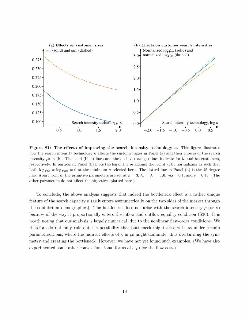
(a) Effects on customer sizes

0.5 1.0 1.5 2.0

0.100

0.125

0.150

0.175

0.200

0.225

0.250

0.275

mlo (solid) and mhn (dashed)

Search intensity technology, κ

(b) Effects on customer search intensities

−2.0 −1.5 −1.0 −0.5 0.0 0.5

0.0

0.5

1.0

1.5

2.0

2.5

3.0Normalized logρlo (solid) andnormalized logρhn (dashed)

Search intensity technology, logκ

Figure S1: The effects of improving the search intensity technology κ. This figure illustrates

how the search intensity technology κ affects the customer sizes in Panel (a) and their choices of the search

intensity ρs in (b). The solid (blue) lines and the dashed (orange) lines indicate for lo and hn customers,

respectively. In particular, Panel (b) plots the log of the ρs against the log of κ, by normalizing as such that

both log ρlo = log ρhn = 0 at the minimum κ selected here. The dotted line in Panel (b) is the 45-degree

line. Apart from κ, the primitive parameters are set at n = 3, λu = λd = 1.0, md = 0.1, and s = 0.45. (The

other parameters do not affect the objectives plotted here.)

To conclude, the above analysis suggests that indeed the bottleneck effect is a rather unique

feature of the search capacity n (as it enters asymmetrically on the two sides of the market through

the equilibrium demographics). The bottleneck does not arise with the search intensity ρ (or κ)

because of the way it proportionally enters the inflow and outflow equality condition (S30). It is

worth noting that our analysis is largely numerical, due to the nonlinear first-order conditions. We

therefore do not fully rule out the possibility that bottleneck might arise with ρs under certain

parametrizations, where the indirect effects of κ in ρs might dominate, thus overturning the sym-

metry and creating the bottleneck. However, we have not yet found such examples. (We have also

experimented some other convex functional forms of c(ρ) for the flow cost.)

18

S5 Transition dynamics

This appendix characterizes the non-stationary equilibria of the model. Doing so allows us to

examine the transition of the endogenous model elements, like the demographics and the welfare,

in between shocks and the eventual steady states. In particular, Section S5.3 shows that when the

discount rate is low, comparing welfare only in steady states (as we do in Section 2.3.3 and 3.3) is

equivalent to comparing also welfare during transition dynamics.

S5.1 Demographics

First, consider the dynamics of high-type customers, η ≡ mho +mhn. The change of η over time,

η is given by inflows (1− η)λu minus the outflows ηλd. Thus, we can write the flow as an ordinary

differential equation (ODE):

η = (1− η(t))λu − η(t)λd.

Solving it with initial condition η(0) = η0 yields the solution

η(t) = η∗ + (η0 − η∗) exp(−(λu + λd)t), (S31)

where η∗ = λuλu+λd

.

Second, one can express all customer masses in terms of mdo, η and mlo. From the non-time-

varying conditions mho +mhn = η, mhn +mln = 1− η, and mho +mlo = s−mdo, we obtain

mho(t) = s−mdo(t)−mlo(t), (S32)

mhn(t) = mlo(t) + η(t)− s+mdo(t), (S33)

mln(t) = 1−mlo(t)− η(t). (S34)

It remains to characterise the dynamics of mlo and mdo. The equations are similar to the

stationary case, but we equalise the difference between inflows and outflows to time derivative of

these masses (which are zero in steady states):

mlo = mho(t)λd −mlo(t)λu − ρmlo(t)νlo(t), (S35)

mdo = ρmlo(t)νlo(t)− ρmhn(t)νhn(t). (S36)

The probabilities νlo(t) and νhn(t) can be expressed through mdo(t) exactly as in the stationary

case. We now summarise the above discussion.

Lemma S2. Consider the system of ODEs (S35) and (S36), given the initial conditions mlo(0) =

mlo,0 and mdo(0) = mdo,0. The solution to this system, combined with (S31)−(S34) fully charac-

terises the demographics in a nonstationary equilibrium, where gains from trade between customers

and dealers exist at all times.

The proof follows the preceding analysis.

19

Solving the demographics reduces to solving the system of two non-linear first-order ODEs (S35)

and (S36), which can be done numerically, using standard methods. We verify that the gains from

trade are positive numerically, as we explain in the next subsection.

S5.2 Value functions

Our derivations are very similar to the stationary case. Consider an ho-bystander. His value

function at time t consists of utility flows over a short time interval dt plus the discounted future

value function, given that there is no exit shock

Vho(t) = yhdt+ λd(Vlo(t)− Vho(t)) + e−(r+fc)dt︸ ︷︷ ︸1−(r+f)dt

Vho(t+ dt)

Taking the limit as dt→ 0 we obtain the HJB

0 = Vho + yh + λd · (Vlo(t)− Vho(t))− (r + fc)Vho(t). (S37)

The HJB is similar to the stationary case. The only difference is that now we have to add Vho at

the right-hand side.

Proceeding similarly we obtain the remaining HJBs

0 = Vln + λu · (Vhn(t)− Vln(t))− (r + fc)Vln(t), (S38)

0 = Vlo + yl + λu · (Vho(t)− Vlo(t))− rVlo(t) + ζlo(t)∆dl(t), (S39)

0 = Vhn + λd · (Vln(t)− Vhn(t))− (r + fc)Vhn(t) + ζhn(t)∆hd(t), (S40)

0 = Vdo + yd − (r + fd)Vdo(t) + ζdo(t)∆hd(t), (S41)

0 = Vdn − (r + fd)Vdn(t) + ζdn(t)∆dl(t). (S42)

Here the trading gains ∆hd and ∆dl as well as trading gains rates ζτ , τ ∈ {lo, hn, do, dn} are

defined exactly as in the stationary case. The above analysis leads to the following lemma:

Lemma S3. Suppose that the reservation values satisfy 0 < Rl(t) < Rd(t) < Rh(t). Then the

value functions are the solution to the system of linear ODEs (S37)-(S42).

To check that there are gains from trade one solves for reservation values, which follow the

following linear ODE system.

0 = Rh + yh − rRh(t)− ζhn(t)(Rh(t)−Rd(t))− λd(Rh(t)−Rl(t)), (S43)

0 = Rl + yl + λu(Rh(t)−Rl(t))− rRl(t) + ζlo(t)(Rd(t)−Rl(t)), (S44)

0 = Rd + yd − rRd(t) + ζdo(t)(Rh(t)−Rd(t))− ζdn(t)(Rd(t)−Rl(t)). (S45)

We summarise our approach to numerically solving for the non-stationary equilibria. First, we

solve for demographics using the results of Lemma S2. Second, we solve for value functions using

Lemma S3. Third, we verify that gains from trade are positive everywhere along the equilibrium

20

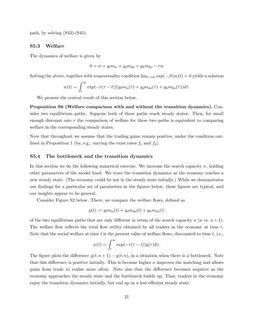
path, by solving (S43)-(S45).

S5.3 Welfare

The dynamics of welfare is given by

0 = w + ylmlo + ydmdo + yhmho − rw

Solving the above, together with transversality condition limt→∞ exp(−βt)w(t) = 0 yields a solution

w(t) =

∫ ∞

texp(−r(τ − t))(ylmlo(τ) + ydmdo(τ) + yhmho(τ))dτ.

We present the central result of this section below.

Proposition S6 (Welfare comparison with and without the transition dynamics). Con-

sider two equilibrium paths. Suppose both of these paths reach steady states. Then, for small

enough discount rate r the comparison of welfare for these two paths is equivalent to comparing

welfare in the corresponding steady states.

Note that throughout we assume that the trading gains remain positive, under the condition out-

lined in Proposition 1 (by, e.g., varying the exist rates fc and fd).

S5.4 The bottleneck and the transition dynamics

In this section we do the following numerical exercise. We increase the search capacity n, holding

other parameters of the model fixed. We trace the transition dynamics as the economy reaches a

new steady state. (The economy could be not in the steady state initially.) While we demonstrates

our findings for a particular set of parameters in the figures below, these figures are typical, and

our insights appear to be general.

Consider Figure S2 below. There, we compare the welfare flows, defined as

y(t) := ylmlo(t) + ydmdo(t) + yhmho(t)

of the two equilibrium paths that are only different in terms of the search capacity n (n vs. n+1).

The welfare flow reflects the total flow utility obtained by all traders in the economy at time t.

Note that the social welfare at time t is the present value of welfare flows, discounted to time t, i.e.,

w(t) =

∫ ∞

texp(−r(τ − t))y(τ)dτ.

The figure plots the difference y(t;n+ 1)− y(t;n), in a situation when there is a bottleneck. Note

that this difference is positive initially. This is because higher n improves the matching and allows

gains from trade to realise more often. Note also that the difference becomes negative as the

economy approaches the steady state and the bottleneck builds up. Thus, traders in the economy

enjoy the transition dynamics initially, but end up in a less efficient steady state.

21

Difference in welfare flows, y(t;n+ 1)− y(t, n)

0 50 100 150 200

-0.004

-0.002

0.000

0.002

time t

Figure S2: Welfare flows in non-stationary equilibria. This figure plots the dynamics of the difference

of welfare flows y(t;n+1)−y(t, n). We set n = 3. The other parameters are set at s = 0.6, md = λd = λu =

λd = r = 0.1, and ρ = 0.01. The initial conditions are given by η(0) = 0.5, mdo(0) = 0.06 and mlo(0) = 0.26.

This figure is typical: for the model parameters where we have bottleneck, the plot starts at zero, is positive

initially, and then crosses zero to reach a negative horizontal asymptote.

TO illustrate the build up of the bottleneck we also look at the transition dynamics of an

incremental change in mdo, mdo(t;n + 1) − mdo(t;n) in Figure S3 Panel (a). One can see that

the increase in n leads to a steady incremental increase in mdo, manifesting the buildup of the

bottleneck. Panel (b) shows the change in the mass of the “most efficient” asset holders mho,

i.e., mho(t;n + 1) −mho(t;n). One can see that it is positive, initially. This is because higher n

means that buyers can meet matching dealers more often, implying better asset flow from dealers

to buyers. This echoes the intuition above that better matching should improve efficiency. But note

that such improvement in efficiency only lasts for a very short period, during which the masses of

traders are roughly unchanged. Over time, however, the equilibrium allocation effect kicks in and

the masses adjust towards the steady state. The bottleneck then builds up, leading to incremental

decrease in mho.

S6 An alternative price-setting mechanism

This appendix considers an alternative price-setting mechanism, where a customer can negotiate

the price with the dealer after the RFQ auction. Specifically, when a customer is in contact with

n dealers, the game proceeds in two steps:

• First, the customer runs a first-price auction among the n dealers.

• Second, the customer bargains with the dealer who has just won the auction, keeping the

option to trade at the dealer’s quote from the auction. The bargaining protocol is as follows:

22

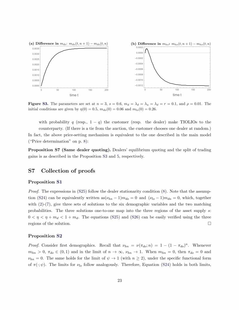
(a) Difference in mdo: mdo(t, n+ 1)−mdo(t, n)

0 50 100 150 200

0.0000

0.0005

0.0010

0.0015

0.0020

0.0025

0.0030

0.0035

time t

(b) Difference in mho: mho(t, n+ 1)−mho(t, n)

0 50 100 150 200

-0.0012

-0.0010

-0.0008

-0.0006

-0.0004

-0.0002

0.0000

0.0002

time t

Figure S3. The parameters are set at n = 3, s = 0.6, md = λd = λu = λd = r = 0.1, and ρ = 0.01. The

initial conditions are given by η(0) = 0.5, mdo(0) = 0.06 and mlo(0) = 0.26.

with probability q (resp., 1 − q) the customer (resp. the dealer) make TIOLIOs to the

counterparty. (If there is a tie from the auction, the customer chooses one dealer at random.)

In fact, the above price-setting mechanism is equivalent to the one described in the main model

(“Price determination” on p. 8):

Proposition S7 (Same dealer quoting). Dealers’ equilibrium quoting and the split of trading

gains is as described in the Proposition S3 and 5, respectively.

S7 Collection of proofs

Proposition S1

Proof. The expressions in (S25) follow the dealer stationarity condition (8). Note that the assump-

tion (S24) can be equivalently written as(νhn − 1)mdo = 0 and (νlo − 1)mdn = 0, which, together

with (2)-(7), give three sets of solutions to the six demographic variables and the two matching

probabilities. The three solutions one-to-one map into the three regions of the asset supply s:

0 < η < η +md < 1 +md. The equations (S25) and (S26) can be easily verified using the three

regions of the solution. □

Proposition S2

Proof. Consider first demographics. Recall that νhn = ν(πdo;n) = 1 − (1 − πdo)n. Whenever

mhn > 0, πdo ∈ (0, 1) and in the limit of n → ∞, νhn → 1. When mhn = 0, then πdo = 0 and

νhn = 0. The same holds for the limit of ψ → 1 (with n ≥ 2), under the specific functional form

of π(·;ψ). The limits for νlo follow analogously. Therefore, Equation (S24) holds in both limits,

23

which then proves the convergence of all demographic variables together with the demographic

conditions (2)-(7).

For value functions and prices, in both limit as n→ ∞ and ψ → 1 (with n ≥ 2), we have perfect

competition among dealers, whenever mdo ∈ (0,md). Thus, pa = pb = Rd and the value function

system is the same as in DS. In the case of mdo = 0 (mdo = md) we have ∆hd = 0 (∆dl = 0) in the

two limits (n→ ∞ and ψ → 1) and so, again, prices and values are as in DS. □

Proposition S3

Proof. The proof only focuses on a contacted do-seller’s symmetric quoting strategy. The same

analysis applies to dn-buyers and is omitted. Consider first the trivial case of n = 1. A contacted

do-seller then knows that he is the only one quoting. It is then trivial that with probability (1− q),he will quote the highest possible ask price, i.e., the hn-buyer’s reservation value Rh = Rd +∆hd.

This can be viewed as a degenerate mixed strategy with c.d.f. F (α) converging to a unity probability

mass at α = 1 as stated in the proposition.

Next consider n ≥ 2. Given the reservation values, it suffices to restrict the ask quote within

[Rd, Rh]. Without loss of generality, a do-seller’s strategy can be written as Rd+α∆hd by choosing

α ∈ [0, 1]. Suppose α has a c.d.f. F (α) with possible realizations [0, 1] (some of which might have

zero probability mass). The following four steps pin down the specific form of F (·) so that it

sustains a symmetric equilibrium.

Step 1: There are no probability masses in the support of F (·). If at α∗ ∈ (0, 1] there is some

non-zero probability mass, any do-seller has an incentive to deviate to quoting with the same

probability mass but at a level infinitesimally smaller than α∗. This way, he converts the strictly

positive probability of tying with others at α∗ to winning over others. (The undercut costs no

expected revenue as it is infinitesimally small.) If at α∗ = 0 there is non-zero probability mass,

again, any do-seller will deviate, this time to an α just slightly above zero. This is because allocating

probability mass at zero brings zero expected profit. Deviating to a slightly positive α, therefore,

brings strictly positive expected profit. Taken together, there cannot be any probability mass in

α ∈ [0, 1]. Note that any pure symmetric-strategy equilibria are ruled out.

Step 2: The support of F (·) is connected. The support is not connected if there is (α1, α2) ⊂ [0, 1]

on which there is zero probability assigned and there is probability density on α1. If this is the case,

then any do-seller will deviate by moving the probability density on α1 to any α ∈ (α1, α2). Such

a deviation is strictly more profitable because doing so does not affect the probability of winning

(if one wins at bidding α1, he also wins at any α > α1) and because α > α1 is selling at a higher

price.

Step 3: The upper bound of the support of F (·) is 1. The logic follows Step 2. Suppose the upper

bound is α∗ < 1. Then, allocating the probability density at α∗ to 1 is a profitable deviation: It

does not affect the probability of winning and upon winning sells at a higher price.

24

Step 4: Deriving the c.d.f. F (·). Suppose all other do-sellers, when contacted, quote according to

some same distribution F (·). Consider a specific seller called i. Quoting Rd+α∆hd, i gets to trade

with the searching buyer if, and only if, such a quote is the best that the buyer receives. The buyer

examines all quotes received. For each of the n−1 contacts, with probability 1−πdo the dealer is nota do-seller and in this case i’s quote beats the no-quote. With probability πdo, the contacted investor

is indeed another lo-seller, who quotes at α′. Then, only with probability P(α < α′) = 1−F (α) willi’s quote win. Taken together, for each of the n − 1 potential competitor, i wins with probability

(1− πdo) + πdo(1− F (α)), and he needs to win all these n− 1 times to capture the trading gain of

α∆hd. That is, i expects a profit of (1− πdoF (α))n−1α∆hd. In particular, at the highest possible

α = 1, the above expected profit simplifies to (1− πdo)n−1∆hd, because F (1) = 1. In a mixed-

strategy equilibrium, i must be indifferent of quoting any values of α in the support. Equating

the two expressions above and solving for F (·), one obtains the c.d.f. stated in the proposition. It

can then be easily solved that the lower bound of the support must be at (1− πdo)n−1, where F (·)

reaches zero. This completes the proof. □

Proposition S4

Proof. Consider a searching hn-buyer, for example. He contacts n dealers but knows that the

number of counterparties he will actually find, N , is a random variable that follows a binomial

distribution with n draws and success rate πdo. Each of these N counterparties then quotes a

random price according to F (α;πdo, n), as stated in Proposition S3. The searching buyer chooses

the lowest ask across the N available quotes. The c.d.f. of this minimum α is 1− (1− F (α; ·))N−1

for N ≥ 1. Since the probability of N ≥ 1 is (1− (1− πdo)n), one obtains the conditional c.d.f. as

stated in the proposition. The same applies to a searching lo-seller. □

Proposition S5

Proof. Consider the limit of ψ → 1 (with n ≥ 2). For anymdo > 0 andmdn > 0, πdo = π(mdomd

)→ 1

and πdn = π(mdnmd

)→ 1. Therefore, the G(·) function in Proposition S4 converges to G(x) = 1

throughout the support of x ∈ (0, 1]. The equilibrium trading prices, therefore, become A → Rd

and B → Rd almost surely, and var[A] → 0 and var[B] → 0 accordingly. That is, in the limit of

ψ → 0, there is no price dispersion. Since the variances are nonnegative, by continuity, therefore,

both var[A] and var[B] must decrease with ψ for sufficiently large ψ. □

25

Proposition S6

Proof. Consider one path and calculate the welfare:

rw(t) = r

∫ ∞

texp(−r(τ − t))(ylmlo(τ) + ydmdo(τ) + yhmho(τ))dτ // letting y := rτ

=

∫ ∞

rtexp(−y + rt)(ylmlo(y/r) + ydmdo(y/r) + yhmho(y/r))dy

r→0−−−→∫ ∞

0exp(−y)(ylmlo(∞) + ydmdo(∞) + yhmho(∞))dy

= ylmlo(∞) + ydmdo(∞) + yhmho(∞)

The last line gives the welfare (in flow terms) in the steady state. The proposition follows. □

Proposition S7

Proof. We start with dealers’ quoting. The proof only focuses on a contacted do-seller’s symmetric

quoting strategy. Without loss of generality, a do-seller’s strategy can be written as Rd + α∆hd

by choosing α ∈ [0, 1]. Suppose α has a c.d.f. F (α) with possible realizations [0, 1] (some of which

might have zero probability mass). The proof, identical to the one for the Proposition S3 can show

that: (i) dealers will quote buyers’ reservation value when n = 1, (ii) for n > 2 dealers would follow

mixed-strategies with no point masses and continuous supports, (iii) the upper bound of support

of F (·) is one. The only non-trivial step is the following:

Step 4: Deriving the c.d.f. F (·). Suppose all other do-sellers, when contacted, quote according to

some same distribution F (·). Consider a specific seller called i. Quoting Rd + α∆hd, i gets to

trade with the searching buyer if, and only if, such a quote is the best that the buyer receives.

The buyer examines all quotes received. For each of the n − 1 contacts, with probability 1 − πdo

the dealer is not a do-seller and in this case i’s quote beats the no-quote. With probability πdo,

the contacted investor is indeed another lo-seller, who quotes at α′. Then, only with probability

P(α < α′) = 1−F (α) will i’s quote win. Taken together, for each of the n−1 potential competitor,

i wins with probability (1− πdo)+πdo(1−F (α)) = 1−πdoF (α), and he needs to win all these n−1

times to capture the trading gain of α∆hd. When the dealer wins, he trades at a markup α, with

probability 1 − q. Indeed, with probability q the customer will extract the full trading gain from

her at the bargaining stage. That is, i expects a profit of

(1− πdoF (α))n−1α∆hd(1− q).

In particular, at the highest possible α = 1, the above expected profit simplifies to

(1− πdo)n−1∆hd(1− q),

because F (1) = 1. In a mixed-strategy equilibrium, i must be indifferent of quoting any values

of α in the support. Equating the two expressions above and solving for F (·), one obtains the c.d.f.

26

stated in the proposition. It can then be easily solved that the lower bound of the support must

be at (1− πdo)n−1, where F (·) reaches zero.

Having established that dealers’ quoting is unchanged under the new trade protocol, the split

of the trading gains follows immediately. This completes the proof. □

References

Bessembinder, Hendrik, Chester Spatt, and Kumar Venkataraman. 2020. “A Survey of the Mi-crostructure of Fixed-Income Markets.” Journal of Financial and Quantitative Analysis 55 (1):1–45.

Chang, Briana. 2018. “Adverse Selection and Liquidity Distortion.” The Review of EconomicStudies 85 (1):275–306.

Cujean, Julien and Remy Praz. 2015. “Asymmetric Information and Inventory Concerns in Over-the-Counter Markets.” Working paper.

Duffie, Darrell, Piotr Dworczak, and Haoxiang Zhu. 2017. “Benchmarks in Search Markets.” TheJournal of Finance 72 (5):1983–2044.

Guerrieri, Veronica, Robert Shimer, and Randall Wright. 2010. “Adverse Selection in CompetitiveSearch Equilibrium.” Econometrica 78 (6):1823–1862.

Lester, Benjamin, Guillaume Rocheteau, and Pierre-Olivier Weill. 2015. “Competing for OrderFlow in OTC Markets.” Journal of Money, Credit and Banking 47 (S2):77–126.

Lester, Benjamin, Ali Shourideh, Venky Venkateswaran, and Ariel Zetlin-Jones. 2018. “Market-making with Search and Information Frictions.” Working paper.

Wright, Randall, Philipp Kircher, Benoıt Julien, and Veronica Guerrieri. 2020. “Directed Searchand Competitive Search: A Guided Tour.” Journal of Economic Literature Forthcoming.

27