Embed Size (px)
Citation preview
J
MARTIN MARIETTA ENERGY SYSTEMS LIBRARIES
3 445b 004^172 3
ORNL/TM-8366
Simultaneous Heat and Mass
Transfer in Absorption ofGases in Laminar Liquid Films
Gershon Grossman
CENTRAL RESEARCH LIBRARY
CIRCULATION SECTION
4500N ROOM 175
LIBRARY LOAN COPYDO NOT TRANSFER TO ANOTHER PERSON
report, send in name with report andthe library will arrange a loan.
Printed in the United States of America. Available fromNational Technical Information Service
U.S. Department of Commerce5285 Port Royal Road, Springfield, Virginia 22161
NTIS price codes—Printed Copy: A05; Microfiche A01
This report was prepared as an account of work sponsored by an agency of theUnited StatesGovernment. Neither the U nited StatesGovernment nor any agencythereof, nor any of their employees, makes any warranty, express or implied, orassumes any legal liability or responsibility for the accuracy, completeness, orusefulness of any information, apparatus, product, or process disclosed, orrepresents that its use wouldnot infringeprivatelyowned rights.Reference hereinto any specific commercial product, process, or service by trade name, trademark,manufacturer, or otherwise, does not necessarily constitute or imply itsendorsement, recommendation, or favoring by the United States Government orany agency thereof. The views and opinions of authors expressed herein do notnecessarily state or reflect those of the United States Government or any agencythereof.
ORNL/TM-8366
Energy Division
SIMULTANEOUS HEAT AND MASS TRANSFER IN
ABSORPTION OF GASES IN LAMINAR LIQUID FILMS
Gershon Grossman
Date Published - September 1982
Contract No. W-7405-eng-26
Oak Ridge National LaboratoryOak Ridge, Tennessee 37830
operated by
Union Carbide Corporationfor the
Department of Energy
MARTIN MARIETTA ENERGY SYSTEMS LIBRARIES
3 445h DD4C117E 3

CONTENTS
LIST OF FIGURES v
LIST OF TABLES vii
NOMENCLATURE ix
ABSTRACT xiil
EXECUTIVE SUMMARY xv
1. INTRODUCTION 1
2. MODEL AND EQUATIONS 5
3. THE LINEAR ABSORBENT 11
4. EXACT SOLUTION 15
5. RESULTS AND DISCUSSION 25
6. HEAT AND MASS TRANSFER COEFFICIENTS 33
7. INTEGRAL SOLUTION 37
8. NUMERICAL EXAMPLE 55
9. CONCLUSIONS 61
REFERENCES 63
ACKNOWLEDGMENTS 65
ill
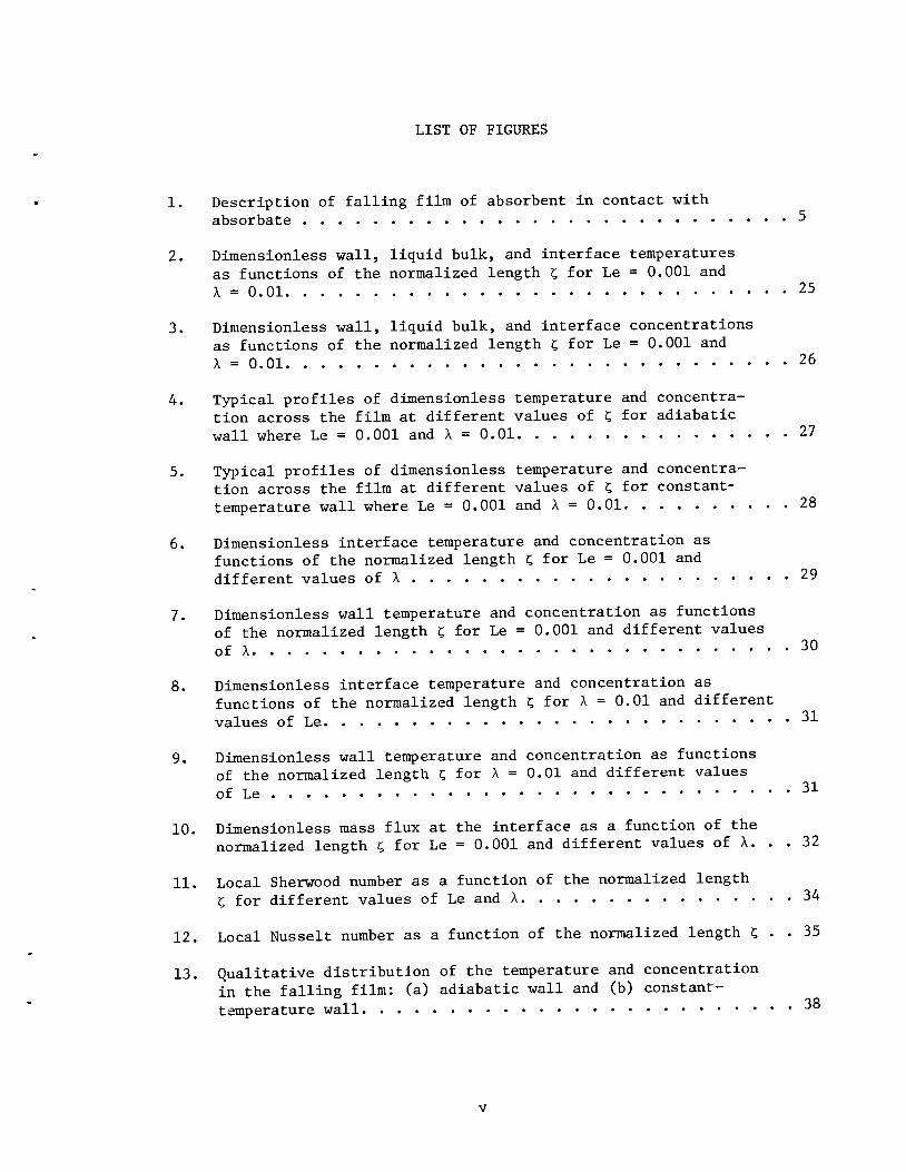
LIST OF FIGURES
1. Description of falling film of absorbent in contact withabsorbate 5
2. Dimensionless wall, liquid bulk, and interface temperaturesas functions of the normalized length t, for Le = 0.001 andA = 0.01 25
3. Dimensionless wall, liquid bulk, and interface concentrationsas functions of the normalized length £ for Le = 0.001 andA = 0.01 26
4. Typical profiles of dimensionless temperature and concentration across the film at different values of t, for adiabatic
wall where Le = 0.001 and A = 0.01 27
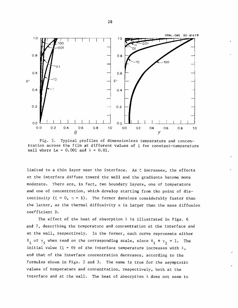
5. Typical profiles of dimensionless temperature and concentration across the film at different values of t, for constant-temperature wall where Le = 0.001 and A = 0.01. 28
6. Dimensionless interface temperature and concentration asfunctions of the normalized length X, for Le = 0.001 anddifferent values of A 29
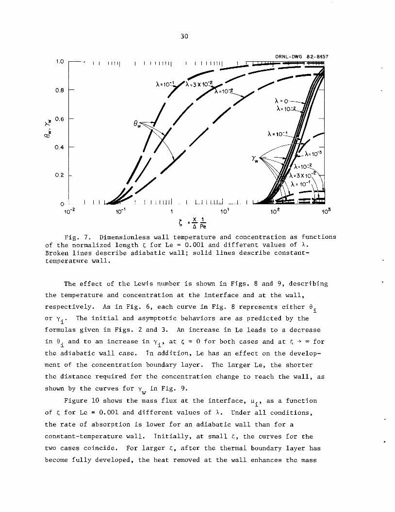
7. Dimensionless wall temperature and concentration as functionsof the normalized length t, for Le = 0.001 and different valuesof A 30
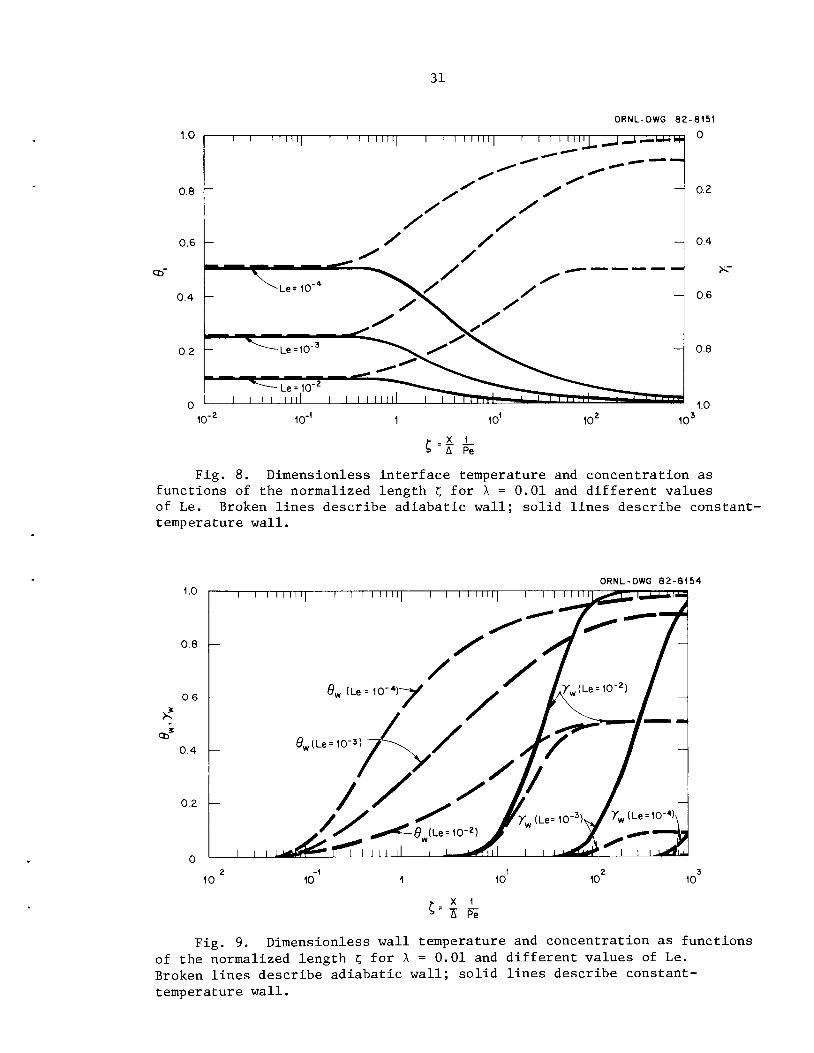
8. Dimensionless interface temperature and concentration asfunctions of the normalized length t, for A = 0.01 and differentvalues of Le 31
9. Dimensionless wall temperature and concentration as functionsof the normalized length c, for A = 0.01 and different valuesof Le 31
10. Dimensionless mass flux at the interface as a function of thenormalized length t, for Le = 0.001 and different values of A. . . 32
11. Local Sherwood number as a function of the normalized lengthc, for different values of Le and A 34
12. Local Nusselt number as a function of the normalized length £ . . 35
13. Qualitative distribution of the temperature and concentrationin the falling film: (a) adiabatic wall and (b) constant-
OQ
temperature wall JO
v
14. Main dimensionless system parameters as functions of the normalized length t, for Le = 0.001 and A = 0.01: (a) boundary layerthicknesses, (b) temperatures, (c) concentrations, and (d) heatand mass fluxes 52
15. Thermodynamic equilibrium chart for LiBr-H„0 solution illustratingthe absorption process with an adiabatic wall and a constant-temperature wall, under the conditions of the numerical example. ... 56
VI
LIST OF TABLES
1. Eigenvalues and coefficients for typical values of theparameters 18
2. Physical properties of LiBr-H„0 solution at 60% concentration and 75°C 57
VII

concentration
NOMENCLATURE
of absorbate in solution [—-j : ;— 1\m° solution /
C — equilibrium concentration of solution at temperature T
•*.t. 4- t> I moles \with vapor at pressure P I —3 ;——:— I
v \ m° solution/
interfacial concentration of absorbate in solution (—q ;—— )\ m° solution/
initial concentration of absorbate in solution (—a ;——:— J\m° solution/
C.1
Co
C. , C„ — constants, Eq. (17a)
/ moles \Im3 solution JC — bulk concentration of absorbate in solution [-^
c — specific heat of liquid (J/kg*°C)P
D — diffusion coefficient of absorbate (substance II) in solution
(m2/s)
H — heat of absorption of substance II in solution (J/mole)a
H — partial molal enthalpy of substance II at interface (J/mole)
h,. — latent heat of evaporation at temperature T (J/kg)fgo r o
\ — mass transfer coefficient from interface to bulk (m/s)
h — heat transfer coefficient from interface to bulk (W/m *°C)
h ' — heat transfer coefficient from bulk to wall (W/m ,0C)
h — enthalpy of vapor in contact with film (J/mole)
IX
k — thermal conductivity of liquid (W/m*°C)
Le — Lewis number (D/a)
M_, M__ — molecular weight of substances I, II I,nnn -.— 1I II ° ylOOO mole/
m — molality of solution (moles electrolyte/kg solution)
n. — mass flux of absorbate into absorbent at interface1
Nu, Nu' — Nusselt number, hyi/k and h 'A/k (dimensionless)
— Peclet number, uA/a (dimensionless)
P — vapor pressure of absorbate (substance II) in the gas phase (Pa)
P — vapor pressure of absorbate (substance II) in solution at
concentration C and temperature T (Pa)
P — vapor pressure of substance II in its pure state (Pa)
P — vapor pressure of substance II in its pure state at
temperature T (Pa)
q — normalized heat flux, [89/8n] _0 (dimensionless)
R — universal gas constant (J/kg*°C)
Sh — Sherwood number, hwA/D (dimensionless)
T — temperature of solution (°C)
(moles ]mz*s /
T — equilibrium temperature of solution at concentration C with
vapor at pressure P (°C)
T. — interfacial temperature of solution (°C)
T — initial temperature of solution (°C)
T — bulk temperature of solution (°C)
u — flow velocity (m/s)
u — average flow velocity (m/s)
v — normalized velocity, Eq. (6) (dimensionless)
x — coordinate in direction of flow (m)
y — coordinate in direction perpendicular to flow (m)
a — thermal diffusivity of liquid (m2/s)
y — normalized concentration, Eq. (6) (dimensionless)
Y — normalized concentration at interface (dimensionless)1
Y — normalized concentration at the wall (dimensionless)w
Y — normalized bulk concentration (dimensionless)
A — film thickness (m)
6 — normalized boundary layer thickness (dimensionless)
6 — normalized concentration boundary layer thickness (dimensionless)Y
6 — normalized thermal boundary layer thickness (dimensionless)
XI
t, — normalized coordinate in direction of flow, Eq. (6) (dimensionless)
5 — value of t, where concentration boundary layer becomes fully
developed (dimensionless)
£q — value of £ where thermal boundary layer becomes fully developed
(dimensionless)
n — normalized coordinate perpendicular to flow, Eq. (6) (dimensionless)
6 — normalized temperature, Eq. (6) (dimensionless)
0. — normalized temperature at interface (dimensionless)
6 — normalized temperature at the wall (dimensionless)w
6 — normalized bulk temperature (dimensionless)
A — normalized heat of absorption, Eq. (10) (dimensionless)
u. — normalized mass flux at interface, Eq. (10) (dimensionless)
v — number of ions in electrolyte (dimensionless)
p — density of liquid (kg/m3)
<f> — osmotic coefficient (dimensionless)
XI1
SIMULTANEOUS HEAT AND MASS TRANSFER IN
ABSORPTION OF GASES IN LAMINAR LIQUID FILMS
ABSTRACT
This report describes a theoretical analysis of the combined heat
and mass transfer process taking place in the absorption of a gas or
vapor into a laminar liquid film. This type of process, which occurs in
many gas-liquid systems, often releases only a small amount of heat,
making the process almost isothermal. In some cases, however, the heat
of absorption is significant and temperature variations cannot be
ignored. One example, from which the present study originated, is in
absorption heat pumps where mass transfer is produced specifically to
generate a temperature change.
The model analyzed in this study describes a liquid film that flows
over an inclined plane and has its free surface in contact with stagnant
vapor. The absorption process at the surface creates nonuniform tem
perature and concentration profiles in the film, which develop until
equilibrium between the liquid and vapor is achieved. The energy and
diffusion equations are solved simultaneously to give the temperature
and concentration variations at the interface and the wall. Two cases
of interest are considered: constant-temperature and adiabatic walls.
The Nusselt and Sherwood numbers are expressed in terms of the operating
parameters, from which heat and mass transfer coefficients can be deter
mined. The Nusselt and Sherwood numbers are found to depend on the
Peclet and Lewis numbers as well as on the equilibrium characteristics
of the working materials.
xm

EXECUTIVE SUMMARY
This report describes the approach to theoretical analysis of the
combined heat and mass transfer process taking place in absorption
systems. The two transfer phenomena are strongly coupled in these
systems. The purpose of the analysis is to relate, quantitatively, the
heat and mass transfer coefficients to the physical properties of the
working fluids and to the geometry of the system. The preferred con
figuration is that of a falling film of liquid on a metallic surface
which transfers heat from the absorbent in contact with the vapor of the
absorbate.
This study originated from ORNL's program on absorption heat pumps.
In trying to optimize the design of absorbers and desorbers for these
systems, it was recognized that fundamental, quantitative information on
the combined heat and mass transfer process was lacking. Correlations
of an empirical nature (not always publicly available) exist for
determining the transfer coefficients for specific fluid pairs in
specific geometries. Theoretical models backed by experimental data
exist on gas absorption in liquid films, but they deal only with iso
thermal mass transfer and neglect the effect of heat transfer. The aim
of the present study has been to produce the kind of fundamental under
standing for the combined process that is already available for pure
heat transfer or pure mass transfer. A theoretical analysis is the
first step in this direction. Our model calculates the temperature and
concentration distributions in the films and the resulting transfer
coefficients for typical flow regimes, geometries, and boundary con
ditions. One of the important results of the analysis is the scaling
laws of the system.
In the system analyzed, a film of liquid solution, composed of
substances I (absorbent) and II (absorbate), flows down over an inclined
plane. The film is in contact with stagnant vapor of substance II at
constant pressure P . At x = 0, the liquid solution is at a uniform
temperature T and composition C (moles of substance II per unit of
volume of solution) corresponding to an equilibrium vapor pressure P
lower than P . As a result of this difference, absorption takes place
xv
at the liquid-vapor interface. The substance absorbed diffuses into the
film, and the heat generated in the absorption results in a simultaneous
heat transfer process. Two cases of practical interest are considered:
in one, the wall is kept at a constant temperature T ; in the other, the
wall is adiabatic.
In formulating the model, the following assumptions have been made:
1. The liquid solution's properties are constant and independent of
temperature and concentration.
2. The mass of vapor absorbed is small compared with the mass flow
rate of the liquid. Therefore, the latter is constant and so is
the film thickness.
3. There is no heat transfer in the vapor phase.
4. There are no natural convection effects in the film due to tem
perature or concentration differences.
5. Diffusion thermal effects are negligible.
6. Vapor pressure equilibrium exists between the vapor and liquid at
the interface.
Under the above assumptions, the simultaneous heat and mass transfer
in the system at steady state is described by the energy and diffusion
equations. Boundary conditions are given (1) at the entrance plane,
x = 0, where the temperature and concentration are known; (2) at the
wall, y = 0, where the no-mass-flux condition requires 3C/3y = 0, and
where either a temperature is specified (for the constant-temperature
wall case) or 9T/3y = 0 (for the adiabatic wall case); and (3) at the
vapor-liquid interface, y = A, where the concentration and temperature
are related to each other through a thermodynamic equilibrium condition,
and the heat flux equals the mass flux times the heat of absorption of
the vapor in the solution. Thus, the two equations can be solved for
the two unknown variables, temperature and concentration, and their
distribution in the film can be obtained.
The model developed is quite general and may be solved for a variety of
flow regimes (laminar, turbulent, transition) and fluid properties. It
can be extended to other wall and interface conditions. In our first
solution, described in this report, the energy and diffusion equations
were solved for laminar flow. A numerical solution based on finite
xvi
differences in a two-dimensional grid and an analytical solution based
on a series of eigenfunctions were developed and agreed very well.
In addition, an integral method was employed which made it possible to
obtain approximate analytical expressions for most parameters of interest.
The solution was carried out for a linear absorbent — a mixture with
a linear temperature-concentration equilibrium relation and a constant
heat of absorption. The techniques of solution are suitable, however,
for nonlinear absorbents with given characteristics.
The solution describes the development of the thermal and concen
tration boundary layers and the variations of the temperatures, concen
trations, and heat and mass fluxes. These quantities in their normalized,
dimensionless forms depend on two characteristic parameters of the
system: the Lewis number Le and the dimensionless heat of absorption A.
The length in the direction of flow is normalized with respect to the
Peclet number and the film thickness.
The model shows the existence of two boundary layers, of temper
ature and of concentration, which develop as the absorption effects at
the interface diffuse toward the wall. The former normally develops
considerably faster than the latter since the Lewis number (ratio of-3
mass to thermal diffusivities) is usually small, on the order of 10 .
The gradients in the temperature and concentration profiles are sharp
for small lengths near the entrance plane and flatten out with distance.
The general dependence of the temperature and concentration on the
normalized length t, = (x/A«Pe) is described in this paper for a typical
set of values of the parameters Le and A. Initially, for small £, the
behavior is the same for both constant-temperature and adiabatic walls.
Thermodynamic equilibrium is reached at the interface immediately upon
contact with the vapor, but it takes some distance for the effect to
diffuse into the film and be felt at the wall. As t, increases, the wall,
bulk, and interface temperatures and concentrations vary toward a final
common value. In the constant-temperature wall case, the dimensionless
temperature and concentration reach asymptotic values of 0 and 1,
respectively. In the adiabatic wall case, the asymptotic temperature
and concentration are A/(A + Le) and Le/(A + Le), respectively.
xvii
Heat and mass transfer coefficients for the system were calculated.
The Sherwood number for mass transfer from the vapor-liquid interface to
the bulk of the film reaches an asymptotic value of 3.45, with fully
developed boundary layers for the constant-temperature wall. Lower
values are obtained for the adiabatic wall. Under the same conditions,
the Nusselt number for heat transfer from the interface to the bulk
reaches values of 4.23 and 2.65 for the adiabatic and constant-tem
perature wall, respectively. The Nusselt number for heat transfer from
the bulk to the wall reaches 1.60.
xvm
1. INTRODUCTION
Absorption of gases and vapors into liquids is encountered in
numerous applications in chemical technology. These processes normally
involve simultaneous heat and mass transfer within the gas-liquid system.
The heat of absorption gives rise to temperature gradients leading to
heat transfer; the temperature influences the vapor pressure and con
centration equilibrium between the two phases, which in turn affects the
exchange of mass.
The combined heat and mass transfer process does not lend itself
easily to mathematical analysis. Many studies of absorption problems
have considered the heat and the mass transfer separately, neglecting
the coupling between them. Fortunately, in many cases the heat inter
action is small, so the process may be considered isothermal. In some
processes, however, the effect of heat transfer is important and cannot
be neglected. A typical example is when the absorbate is a vapor with
high heat of absorption, such as water. Furthermore, there is growing
interest in processes in which mass transfer is initiated specifically
to produce a temperature change. One such example, from which this
study originated, is of absorption heat pumps for heating and cooling;
the heat transfer accompanying the mass transfer is of primary importance.
The gas-liquid contactors in which absorption takes place are
typically spray, trayed, or packed towers. Of particular interest are
systems involving falling liquid films, which have found wide applica
tion in modern equipment. Many studies, using different flow regimes,
geometries, and boundary conditions, have been performed on gas absorp
tion in liquid films. Chien and Ibele did a comprehensive survey of the
hydrodynamics of falling films.1 As early as 1940, Vyazovov formulated
a simple model for isothermal absorption in a falling film, which was
shown by comparison with experimental results to provide rough estimates
for the mass transfer coefficients.2 Improved and more elaborate models
have been since developed. Olbrich and Wild provided a solution to the
diffusion equation in laminar flow for several falling film geometries;
the solution, in the form of a series of eigenfunctions, includes ten
eigenvalues and coefficients.3 Rotem and Neilson added to the laminar
solution the diffusion in the direction of flow, which turns out to be
negligible for large enough Peclet numbers.4 Tamir and Taitel extended
the laminar flow solution to cases involving interfacial resistance.5
Chavan and Mashelkar et al. considered absorption in non-Newtonian
liquids, and Sandall and his co-workers studied turbulent flows.6-10
All these studies deal with mass transfer only, under conditions where
heat transfer has no effect.
Only recently has some work been published on combined heat and
mass transfer in falling films. Yih and Seagrave analyzed a laminar
flow problem and studied the effect of a temperature gradient on the
absorption process.11 Neglecting temperature variations in the direction
of flow, they essentially assumed a linear temperature profile across
the film thickness. The temperature variation in their model influenced
the process through its effect on the physical properties of the liquid.
Nakoryakov and Grigor'eva used a similar approximate approach and also
assumed a linear temperature profile across the film.12 In their model,
however, temperature variations in the direction of flow were not
neglected. Two later and improved models by the same authors have
calculated, rather than assumed, the actual shape of the temperature
profile, which led to more accurate results.13'14 In ref. 13 an eigen-
function series solution is given for the coupled diffusion and energy
equations for an impermeable, constant-temperature wall and an equi
librium boundary condition at the liquid-vapor interface. In ref. 14 an
analytic solution was obtained for the temperature and concentration
variation near the entrance region. The main limitation of these models
is their assumption of a uniform velocity profile in the film, whereas
the actual velocity profile in laminar flow is parabolic. This assumption
leads to a deviation of about 20% in the heat and mass transfer coefficients
and to underprediction by about 40% of the distance required for boundary
layer development. The models are also restricted to a constant-temperature
wall.13'14
The present study originated from work at Oak Ridge National Laboratory
(ORNL) on absorption heat pumps. Although some scattered data are avail
able on the design of absorbers and desorbers for these systems, it was
recognized that fundamental, quantitative information on the combined
heat and mass transfer process is lacking. This report is an attempt to
improve on the models described earlier and to remove some of their
limitations. The model, for a falling film of absorbent solution in
laminar flow, calculates the heat and mass transfer coefficients for
typical wall conditions and finds their dependence on the system's
parameters.

2. MODEL AND EQUATIONS
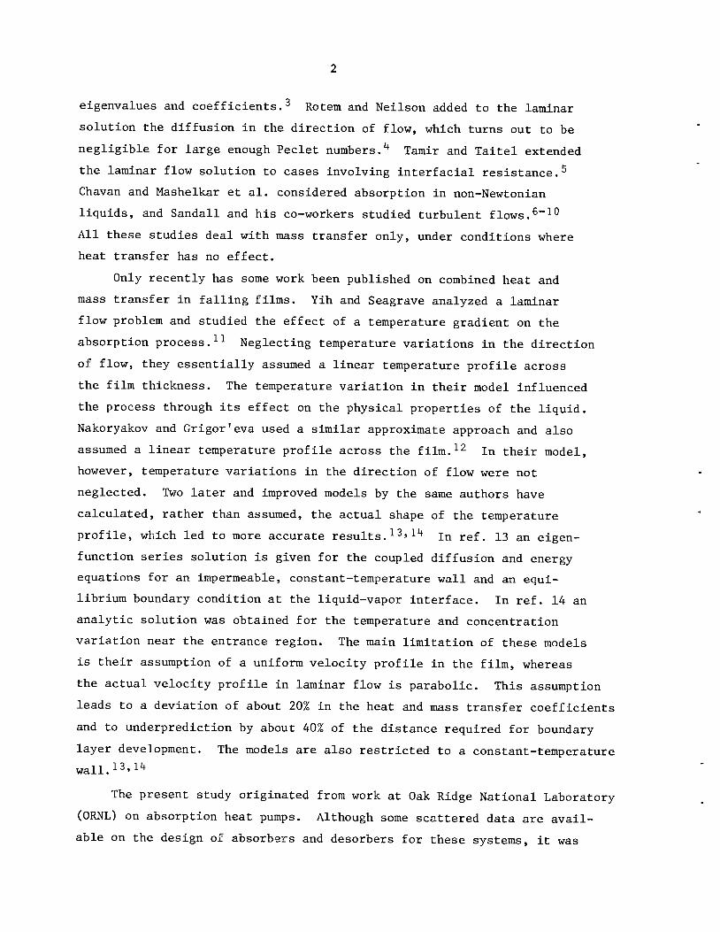
The system analyzed is described schematically in Fig. 1. A film
of liquid solution, composed of substances I (absorbent) and II (absorbate),
0RNL-DW6 81-4736R
T = T
LIQUID
SOLUTIONOF SUBSTANCES
IANDTI
VAPOR OF SUBSTANCE HAT CONSTANT PRESSURE P%
Fig. 1. Description of falling film of absorbent in contact withabsorbate. Typical profiles of velocity, temperature, and concentrationare shown.
flows down over an inclined plane. Substance I remains in the liquid
phase; substance II may be absorbed into the solution. The film is in
contact with the stagnant vapor of substance II at constant pressure P .v
At x = 0, the liquid solution is at a uniform temperature T and com
position C (moles of substance II per unit volume of mixture) corre
sponding to an equilibrium vapor pressure P different from P . Becausevo v
of this difference, a mass transfer process takes place at the liquid-
vapor interface. The substance absorbed at the interface diffuses into
the film; the heat generated in the absorption results in a simultaneous
heat transfer process. Two cases of practical interest are considered:
in one, the wall is kept at a constant temperature T ; in the other, the
wall is adiabatic.
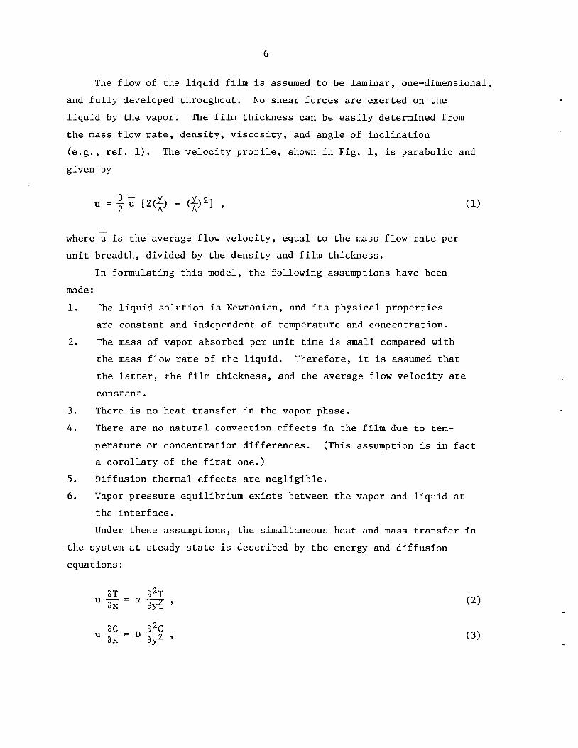
The flow of the liquid film is assumed to be laminar, one-dimensional,
and fully developed throughout. No shear forces are exerted on the
liquid by the vapor. The film thickness can be easily determined from
the mass flow rate, density, viscosity, and angle of inclination
(e.g., ref. 1). The velocity profile, shown in Fig. 1, is parabolic and
given by
u=|u [2(J) -(^)2] , (1)
where u is the average flow velocity, equal to the mass flow rate per
unit breadth, divided by the density and film thickness.
In formulating this model, the following assumptions have been
made:
1. The liquid solution is Newtonian, and its physical properties
are constant and independent of temperature and concentration.
2. The mass of vapor absorbed per unit time is small compared with
the mass flow rate of the liquid. Therefore, it is assumed that
the latter, the film thickness, and the average flow velocity are
constant.
3. There is no heat transfer in the vapor phase.
4. There are no natural convection effects in the film due to tem
perature or concentration differences. (This assumption is in fact
a corollary of the first one.)
5. Diffusion thermal effects are negligible.
6. Vapor pressure equilibrium exists between the vapor and liquid at
the interface.
Under these assumptions, the simultaneous heat and mass transfer in
the system at steady state is described by the energy and diffusion
equations:
9T 32T
U 3i = a W- ' (2)
3C „ 32CU to - DW ' (3)
where diffusion and heat conduction in the x-direction have been neglected
with respect to those in the y-direction. The following boundary condi
tions apply:
or
T = T and C = C at x = 0 ; (4a)o o
^- = 03y u '
T = T for constant temperature wall ,
3T/3y = 0 for adiabatic wall ,
at y = 0 ; (4b)
T = T. and C = C. at y = A . (4c)
Here T. and C. are the interfacial temperature and concentration, both
unknown functions of x. They are related to each other and to the
interfacial mass flux n., also unknown, by the following conditions:
F(T., C.) = P = constant , (5a)1 1 v
D(3C/3y) = n. at y = A , (5b)
k(3T/3y) = n.H (T., C.) at y = A , (5c)X 3. X X
where H is the heat of absorption, per mole of the vapor, in thea
liquid. Equation (5a) represents the condition of vapor pressure equi
librium at the interface; Eqs. (5b) and (5c) describe the mass and heat
fluxes, respectively, at the interface. The heat of absorption is
defined as
H = hTT - H (C , T ) , (5d)a II 11 l l
where h is the enthalpy (per mole) of the vapor in contact with the
film and H is the partial molal enthalpy of substance II at the inter-
face. The variable H is a function of the interfacial temperature and
concentration, whereas h is independent of them. The definition (5d)
is more rigorous than the one sometimes found in the literature, in
which H is expressed in terms of the latent heat of vaporization and3.
condensation of substance II at temperature T. minus the differential
heat of dilution. This definition would be correct if the vapor were
saturated at a temperature equal to that of the liquid interface, but
this is generally not the case, nor is it so in the present problem.
The typical shapes of the temperature and concentration profiles in
the film are depicted in Fig. 1. Before proceeding with the solution,
it would be useful to rewrite the equations in a dimensionless form.
The new variables are defined as
1 x y ,. .? = PeA' nA; <6a>
v=u/u =|(2n -n2) ; (6b)T - T C - C
9 " t~^T ' Y ="c-^"^ ; (6c)e o e o
where T is the equilibrium temperature of the solution at concentration
C with the vapor, and C is the concentration of the solution ato e
temperature T in equilibrium with the vapor. The variables T and C° e e
have a physical significance: T is the temperature the film would
reach if thermodynamic equilibrium could be achieved without change in
concentration, C is the concentration that would be reached if thermo
dynamic equilibrium could be achieved without change in temperature.
Both are limiting cases to what actually happens in the simultaneous
heat and mass transfer process.
Equations (2) and (3), with the new dimensionless variables, become
36
V H =32e3n2 '
v^ = Lef%3rT
(7)
(8)
where Le is the Lewis number. The boundary conditions now have the
dimensionless form
6 = 0 and y = 0 at z, = 0 ; (9a)
or
^ = 0 •3n U '
0 = 0 for constant temperature wall, ) at r\ = 0 ; (9b)
30/3n = 0 for adiabatic wall,
6=0. and Y = Y- at n = 1 ; (9c)
where 0. and y. are the dimensionless interfacial temperature andi l
concentration, both unknown functions of £,, which are related to each
other as follows:
f(0-5 Y-) = 0 (equilibrium condition) , (10a)
n.A
3Y/3n =y± =p* _c) at n=1, (10b)e o _
afl H (C - C )|i -U.A(0., Y)=y.Le a e_T° atn-1. (10c)
p e o
Here y. is the dimensionless mass flux from the vapor to the film and A
is the dimensionless heat of absorption, which is a function of 0. and
VThe problem is now well defined mathematically in terms of the two
second-order differential Eqs. (7) and (8) and the boundary conditions
(9a-c) for the unknown distributions of 0 and y with t, and n. The
boundary conditions are given in terms of two additional unknowns, 0.
and Y-» which are determined along with y. from Eqs. (lOa-c).
The two cases for which the model was developed (constant-temperature
and adiabatic walls) are of practical interest in actual working systems.
The former simulates a process in which the liquid is constantly cooled
during absorption, such as in absorption chillers and heat pumps. The
10
latter represents a case in which the process occurs without cooling,
such as in many gas-liquid contactors. We have assumed that the constant-
temperature wall is at temperature T equal to that of the entering
solution. If this is not the case, the results will vary somewhat because
of an additional pure heat transfer process between the wall and the
film near the entrance region.14 Also, the adiabatic wall may be con
sidered as a particular case of the more general constant heat flux
condition.
3. THE LINEAR ABSORBENT
To proceed with the solution, it is necessary to know the equi
librium relation between the temperature, composition, and vapor pressure
of the specific liquid absorbent being used. This relation, expressed
in a dimensionless form for the parameters at the interface, yields
Eq. (10a). In addition, it is necessary to express the dimensionless
heat and absorption A in terms of 6. and y. for the given materials.
Data on equilibrium properties have been compiled from experimental and
theoretical studies and are available in the literature for many liquid-
vapor combinations.
A universal relation between the temperature, concentration, and
vapor pressure in equilibrium can be formulated which would fit a large
number of absorbents within a limited range of the preceding parameters.
This relation indicates a linear dependence between the temperature, the
concentration, and the logarithm of the vapor pressure. A thermodynamic
justification for this relation, limited to electrolytic solutions, is
given below, based on the definition of the osmotic coefficient and the
Clapeyron equation. Similar behavior is exhibited by some other, non-
electrolytic absorbents.
The osmotic coefficient f of a solution composed of a solvent
(substance II) and a single electrolyte (substance I) which dissociates
into v ions is defined by ref. 15:
1000 , , , ,,,,-<j>vm = —— In (a ) , (11)II
where m is the molality of the solution, related to the solvent con
centration C by
1 MIICm = i- (1000 - -ii-) . (12)M p
The activity of the solvent a may be expressed in terms of the
vapor pressure as
aTT = P /P ° , (13)II v v
11
12
where P is the vapor pressure of substance II in its pure state, at
the given temperature. Substituting Eqs. (12) and (13) into Eq. (11)
yields
P MTTIn = -<£v -—
P ° MIv
(X "IW)- <14>The vapor pressure of the pure substance II may be expressed in
terms of temperature by means of the Clapeyron equation:
P° hfln P^ =RT^ <T "V » (15)
o o
where P is the vapor pressure at the temperature of origin T , and hf
is the latent heat of vaporization at this temperature, assumed to
remain constant over a limited temperature range. The same assumption
can be applied to the osmotic coefficient. Thus, by adding Eqs. (14)
and (15), we obtain the following linear relation between the temperature,
concentration, and logarithm of vapor pressure:
1 Pv * ^In p- - -*v —o I
(CM \ h
The validity of Eq. (16) was checked for a number of common ab
sorbents, including LiBr-H„0, LiCl-H„0, and CaCl„-H20, and was found to
be very good under the above limitations for a wide range of temperatures
and concentrations. It should be noted that for ideal solutions or very
dilute solutions, Raoult's Law or Henry's Law may be applicable instead
of Eq. (16).
The heat of absorption has been defined as the difference between
the enthalpy of the vapor h and the partial molal enthalpy of sub
stance II in the liquid E^ [Eq. (5d)]. The value h ,which is independent
of the interfacial temperature and concentration, is often considerably
larger than H . This is particularly so for vapors of low molecular
weight such as Ho0. In those cases, the dependence of A on 6. and v. is^ 11
very weak.
We will define a linear absorbent as a material having the following
properties:
13
1. The relation between the temperature and concentration in equi
librium with vapor at constant pressure is linear, of the form
C = C^ + C2 . (17a)
2. The heat of absorption is constant and independent of the
temperature and concentration.
Then, for a linear absorbent, the dimensionless relation (10a) becomes
Y± = 1 - 0. , (17b)
and
A = constant . (17c)
4. EXACT SOLUTION
Two different methods of reaching a solution were used to obtain
the temperature and concentration distributions in the film: analytical
and numerical. A linear absorbent was assumed in both cases, and the
results of the two methods were in excellent agreement. The equations
in effect are (7) and (8) with the boundary conditions (9a) and (9b) at
the entrance plane and the wall, respectively. The condition (9c) at
the interface for the case of a linear absorbent becomes
0+ Y=1and |£- = Xp- at n=1 . (18)dri dri
4.1 Analytical Solution
The approach to the solution is similar to the one employed in
ref. 13 for the case with the uniform velocity profile. Using the
Fourier method, we write a separation-of-variables solution for Eqs. (7)
and (8), in the form of two infinite series of eigenfunctions, as follows:
00 -a 2t,
6= L Vn(n)e n » <19a)n=l
-3 2?
Y=1- £ BnGn(n)e n ' <19b)n=l
where a and 3 are the eigenvalues corresponding to the eigenfunctions
F and G , respectively. The boundary conditions (18), which must be
satisfied at any ?, indicate that for every n, a = 3 . Substitutingn n
Eqs. (19a) and (19b) into (7) and (8), we obtain the following equations
for the eigenfunctions:
^ +f(2n-n2)c*n2Fn =0, (20)d2G a 2
-^ +|(2n -n2)^ G =0 , (21)dnz 2V ' ' 'Le n
15
16
with the boundary conditions at the wall resulting from Eq. (9b)
Gn'(0) = 0 ; (22a)
F '(0) =0 for adiabatic wall, or F(0) = 0 for constant
temperature wall. (22b)
Another boundary condition to be satisfied by Eqs. (20) and (21) is
condition (18) at the interface, which yields
A F (1) = B G (1) , (23a)nnnn v '
AF'(l) = -AB G '(1) . (23b)nnnn v '
Note that equations (23a) and (23b) for A and B are homogeneousn n
and have a solution only if the determinant equals zero, namely
Fn'(l) Gn'(l)F (1) = "XG (1) ' <24>
n n
which is the condition for determining the eigenvalues a once a solutionn
is obtained for F and G . The coefficients A and B can then ben n n n
determined from the boundary condition (9a) by means of a Sturm-Liouville
orthogonality condition at Z, = 0.
A power series solution to Eq. (20) may be written in the form
Fn(n) = E A n1 > (25a)i=0 n,x
where, using the boundary condition (22b) , we find
a n = 1, a = 0, a = 0, a „ = -a 2/2 for adiabatic wall ;n,u n,l n,2 n,3 n '
a_ = 0, a n = 1, a 0 = 0, a „ = 0n,0 n,l n,2 ' n,3
for constant-temperature wall ;
3 (an i-4 " 2an i-3)an ±=jan2 '±.± _ 1. > for i5 4, both types of wall . (25b)
17
Similarly, the solution to Eq. (21) may be written as
CO
Gn(n) = E \t±^ > <26a>
where we find, with the aid of boundary condition (22a) ,
b = 1, b = 0, b „ = 0, b = -a 2/2Le ;n,0 n,l n,2 n,3 n
b .=|^~ n^T4 „ n^-3 for 15 4.n,i 2 Le 1(1 - 1)
(26b)
The eigenvalues are the roots of Eq. (24) . An algorithm may there
fore be employed where a guessed value of a is used in Eqs. (25b) and
(26b) to calculate the terms of the series a . and b ., and, hence,v ' n,i n,i
the eigenfunctions F (1) and G (1). The results are then substituted inn n
Eq. (24). If the latter is not satisfied, a different guess is taken
until convergence is obtained.
Table 1 lists the first nine eigenvalues for a set of typical
values of the parameters, A = 0.01 and Le = 0.001. The table also shows
the corresponding coefficients A and B , which must be calculated to
complete the solution. To do so, we must formulate an orthogonality
condition at t, = 0, which is of the Sturm-Liouville type yet somewhat
different from its standard form because of the coupled boundary con
dition in Eq. (18).
Consider Eq. (20) for the eigenfunction F ; multiplying it by
another eigenfunction F and integrating over the range of n yields
4a2/ (2n -n2)F F dn =-/I n J m n J
0
1
F F' dnm n
/= F (O)F' (0) - F (l)F' (1) + / F1 F1 dn . (27a)m n m n / m n
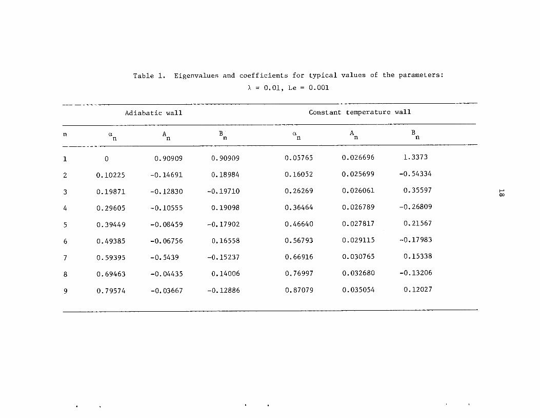
Table 1. Eigenvalues and coefficients for typical values of the parameters:
A = 0.01, Le = 0.001
Adiabatic wall Constant temperature wall
n an
An
Bn
an
An
Bn
1 0 0.90909 0.90909 0.05765 0.026696 1.3373
2 0.10225 -0.14691 0.18984 0.16052 0.025699 -0.54334
3 0.19871 -0.12830 -0.19710 0.26269 0.026061 0.35597
4 0.29605 -0.10555 0.19098 0.36464 0.026789 -0.26809
5 0.39449 -0.08459 -0.17902 0.46640 0.027817 0.21567
6 0.49385 -0.06756 0.16558 0.56793 0.029115 -0.17983
7 0.59395 -0.5439 -0.15237 0.66916 0.030765 0.15338
8 0.69463 -0.04435 0.14006 0.76997 0.032680 -0.13206
9 0.79574 -0.03667 -0.12886 0.87079 0.035054 0.12027
CD
19
Similarly,
4a2 / (2n -n2)F F dn =F (O)F' (0) -F (l)F' (1)2 m J n m n m n mv '
0
1
/ 'V+ / F' F' dn . (27b)J n m
0
Subtracting Eq. (27b) from (27a) and using the boundary condition
(22b), we obtain
.1
3' 2 _ „ 2\ / /o„ _ «2/(a/ - aJ) I (2n - nz)F F dn = F (l)F' (1) - F (l)F' (1) . (28a)z n m j nm nm mn
0
Repeating the same with Eq. (21) for the eigenfunction G , wen
find that
£- (a z - am^) / (2n - nz)G G dn = G^CDG' (1) - Gm(l)G' (1) . (28b)ZLe n m J nm nm mn
0
At this point we introduce the coupling between the equations, which is
where this orthogonality condition differs from the conventional one.
From Eqs. (23a) and (23b),
F (l)F' (1) - F (l)F' (1) = -A-^ [G (l)G' (1) - G (l)G' (1)] ;nm mn AAnm mn
n m
using this condition to combine Eqs. (28a) and (28b) finally yields
ar,2 " O / ^ ~ n2)GJn m J n
-r(a 2 - a 2) / <2n - n2)(LeA AF F + AB B GG ) dn = 0 , (29a)n m J nmnm nmnm
0
which may be written as
= 0 for n 4- m
/ (2n - n2)(LeA AFF +ABBGG)dn_ nmnm nmnm 4- 0 for n = m
(29b)
It should be noted that this type of "coupled" orthogonality condition
was developed and used earlier by Sparrow and Spalding in a problem
involving sublimation in a duct.16
20
We now return to boundary condition (9a); using Eq. (19), we find
CO oo
J2 Vn(n) =° and T BnGn(n) =1 ; (30)n=l n=l
therefore,
y> / (2n - n2)(LeA AFF +ABBGG)dni_j J nmnm nmnmn=l 0
= J (2n - n2);iXB G dn . (31a)„ m m v '
Using the orthogonality condition (29b),
J (2n - n2)(LeA 2F 2+ AB 2G 2) dn = J (2n -n0 nn n n ' *: ' n n2)AB^G^ dn ,
(31b)
which provides one relation between A and B ; a second relation is avail-n n
able in either (23a) or (23b). Solving (31b) and (23a) for A and B yieldsn n J
xJ (2n - n2)Gn(n) dn0
B = , (32a)
f Gn2^Jq (2n - n2)[Lef\^y Fn2(n) +AGn2(n)] dn
G (1)
An - Bn FTiy * (32b)n
The analytical solution is now complete. The algorithm mentioned
earlier makes it possible to obtain the first few eigenvalues* from
Eq. (24) without difficulty for most values of interest of the parameters.
This is sufficient for an accurate calculation of 0 and y for moderate
and large values of £ due to the exponential terms in Eqs. (19a-b). For
*The sequence of the eigenvalues is such that a higher n correspondsto a larger value of a .
n
21
small values of z,, however, a large number of eigenvalues is required.
The recursive formulas (25b) and (26b) turn out to be unstable for large
values of a , and it is increasingly difficult to obtain convergence of
the series (25a-b) and (26a-b) for the eigenfunctions. An alternative
method for obtaining the eigenvalues is through a numerical integration
of Eqs. (20) and (21). Rather than doing this, it was found to be more
efficient to use a numerical method for solving the original Eqs. (7)
and (8) in their partial differential forms, which will be described
next. Yet, the analytical eigenvalue solution is very useful for a wide
range of the parameters Le and A, where enough eigenvalues can be cal
culated to cover a considerable range of £. For the small ?'s, a simi
larity solution has been obtained similar to the one in ref. 14, which
will also be described below.
4.2 Numerical Solution
The numerical technique used to solve the partial differential
Eqs. (7) and (8) was based on the so-called "method of lines" or "semi-
discretization."17 The z, - n plane of the film was divided into thin
strips by means of lines parallel to the z, axis. This discretization of
the n-coordinate made it possible to express the second-order derivative
with respect to n in each of the equations in a finite-difference form.
Thus, a first-order ordinary differential equation, in z. alone, was ob
tained along each line. Such an equation could be readily solved by
means of an available ordinary differential equation integrator using
the boundary condition (9a). The integrator selects automatically the
required step in z, and varies it as necessary as the integration proceeds.
Some difficulty in applying this numerical method to the entire
domain resulted from a singularity at the point Z, - 0, n = 1. This is a
singularity of the type often encountered in boundary layer problems and
is due to a discontinuity in the temperature and concentration between
the interface and the entrance plane at this point. To overcome this
problem, an analytical solution applicable close to the singular point
was developed, which made it possible to calculate the values of the
variables at some finite distance away from the point and begin the
22
numerical solution from there. The analytical solution is similar to
the one used in ref. 13 and will be described briefly here.
By defining a new variable
n1 = l - n , (33)
and recognizing that the term (2n - n2) is very close to unity near the
singular point, we can rewrite Eqs. (7) and (8) as
3 30 32(2 3£ 3n T ' (34)
!&-*%• «5>where the boundary conditions (9b) and (18) now apply at n., ""*" °° and
n, = 0, respectively. It is then possible to find a similarity variable,
combining both z, and n-, > for each of the equations and to convert them
from partial to ordinary ones. Using the common similarity technique,
Eq. (34) becomes
d20 „ d6dz^ " "2Z dz" > <34a>
where z= n1/'\/8c/3. Eq. (34a) may be integrated twice to give
6= k± erf (z) + k2 = k± erf (^^8^/3 )+ k, . (34b)
In a similar manner we find from Eq. (35) that
Y=k3 erf (r^/V'8Le?/3) +k4 , (35a)
where k^, k2, k„, and k, are constants of integration. Applying the
boundary condition (9a) yields k = -k and k = -k, since erf (°°) = 1.
The boundary condition (9b) is satisfied automatically for both the
adiabatic and constant-temperature walls. Then, applying the boundary
condition (18) yields k± + k3 =-1 and k± =Xk^yfhe from which all theconstants of integration can finally be determined. Thus, we obtain the
23
following expressions for the dimensionless temperature and concentrations,
in terms of the original variables:
Y
A + yfHe
Vl7A+y,Le
1-erf Y
1 - erf "If
' 3(1 - n)28£
/3(1 - n)28Le£
(36)
(37)
which are valid for small z,, for both the adiabatic and constant-tempera
ture wall cases. This is to be expected, since the effect of the wall
cannot be felt until the boundary layer developing from the interface
has had enough distance to fill the entire film thickness.
The similarity solution for a small value of Z, has made it possible
to use the numerical technique described earlier and to overcome the
problem associated with the discontinuity at the point z, = 0, n = 1. In
addition, this solution is used to complement the eigenvalue solution
whose usefulness at small z, was limited by the number of obtainable
eigenvalues.

5. RESULTS AND DISCUSSION
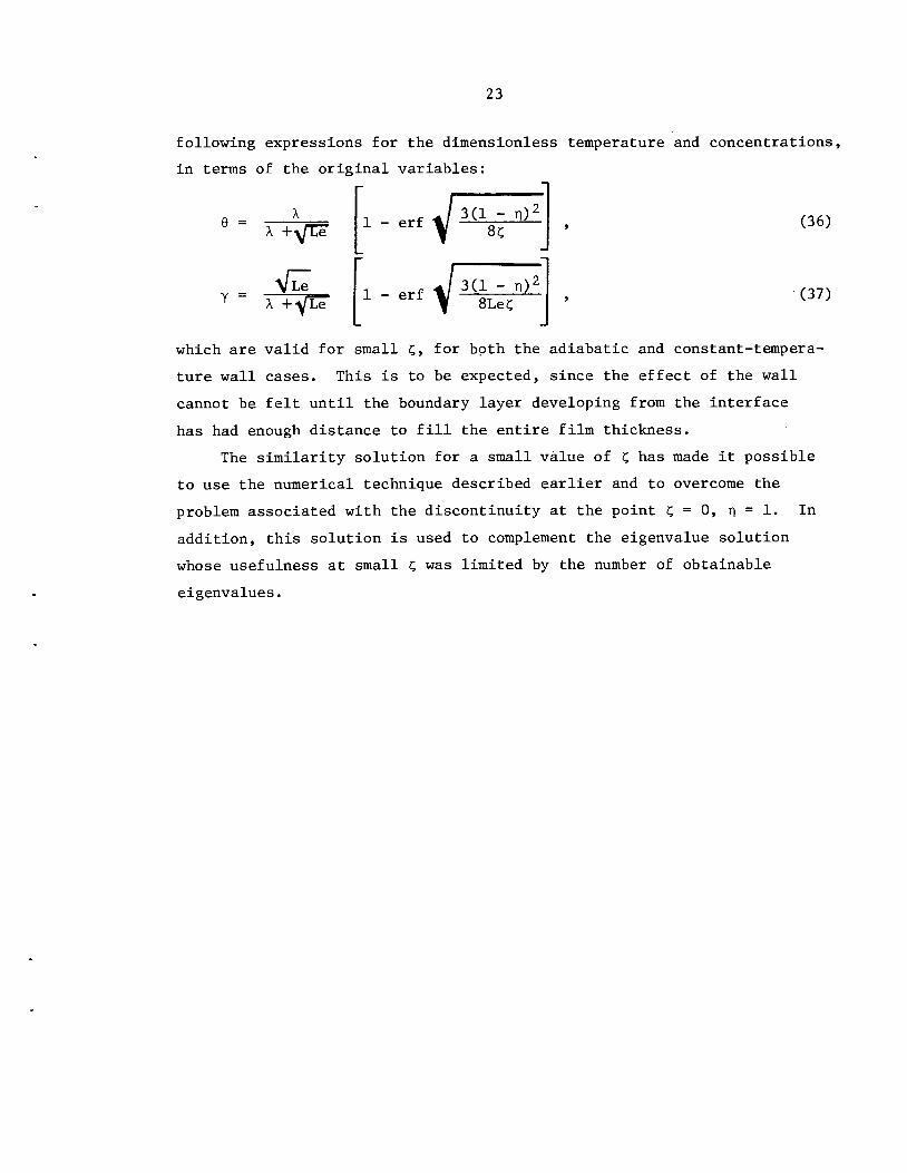
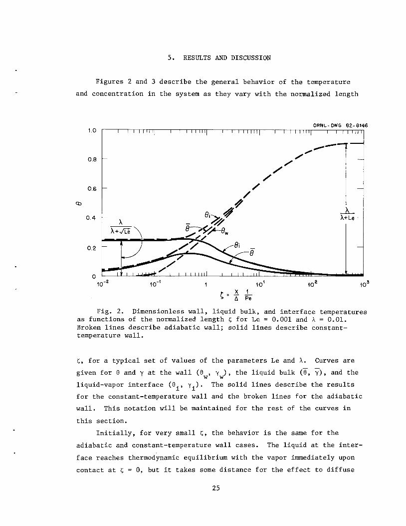
Figures 2 and 3 describe the general behavior of the temperature
and concentration in the system as they vary with the normalized length
1.0 I | I I I I I I II I I I I | II II 1 1—TTTTORNL-DWG 82-8146
CD
0.4 -
Fig. 2. Dimensionless wall, liquid bulk, and interface temperaturesas functions of the normalized length Z, for Le = 0.001 and A = 0.01.
Broken lines describe adiabatic wall; solid lines describe constant-
temperature wall.
z,, for a typical set of values of the parameters Le and A. Curves are
given for 6 and y at the wall (0 , Y )» the liquid bulk (0, y), and thew w
liquid-vapor interface (6., y.). The solid lines describe the results
for the constant-temperature wall and the broken lines for the adiabatic
wall. This notation will be maintained for the rest of the curves in
this section.
Initially, for very small z,, the behavior is the same for the
adiabatic and constant-temperature wall cases. The liquid at the inter
face reaches thermodynamic equilibrium with the vapor immediately upon
contact at z, = 0, but it takes some distance for the effect to diffuse
25
1.0
0.8 -
0.6 —
X
0.4
0.2 —
10" 10"
26
£x. J_A Pe
101
ORNL-DW6 82-8145
10' 10-
Fig. 3. Dimensionless wall, liquid bulk, and interface concentrations as functions of the normalized length z, for Le = 0.001 andA = 0.01. Broken lines describe adiabatic wall; solid lines describeconstant-temperature wall.
into the film and be felt at the wall. Consequently, 0 and y remainw w
essentially zero for small z, while 0. and Y- remain almost constant at
their initial values reached at r, = 0. These values are A/(A +*fhe)and-^Le/(A +-JLe) , respectively, as we find from the similarity solutionfor small E,, Eqs. (36) and (37).
As C increases for the adiabatic wall case, the wall, bulk, and
interface temperatures increase monotonically toward a final common
value and become closer and closer to each other. This steady increase
occurs because the heat of absorption is not being removed from the
system. For the constant-temperature wall, the interface temperature
increases slightly, following the trend of small t,, and the bulk tem
perature attempts to approach it as heat is conducted from the interface
into the film. Then, both temperatures decrease toward zero as heat
flows out of the system through the wall. The interfacial concentration
in both cases follows a trend opposite to that of the interfacial tem-
27
perature, since y. - 1 - 0. [Eq. (18)]. The bulk concentration increases
in both cases toward a final value equal to that of y.. Note that in the
adiabatic wall case y increases with z,, while y« decreases.
The asymptotic values of the dimensionless temperature and con
centration may be found from the eigenvalue solution by substituting
z, -> oo in Eqs. (19a-b). In the constant-temperature wall case, the
dimensionless temperature becomes equal to that of the wall (0 = 0),
and the concentration reaches the corresponding equilibrium value (y = 1).
In the adiabatic wall case, the asymptotic temperature reflects some
increase from the initial value [0 = A/(Le + A)], and the corresponding
equilibrium concentration [y = Le/(A + Le)] is lower than the thermo-
dynamically possible value of 1.
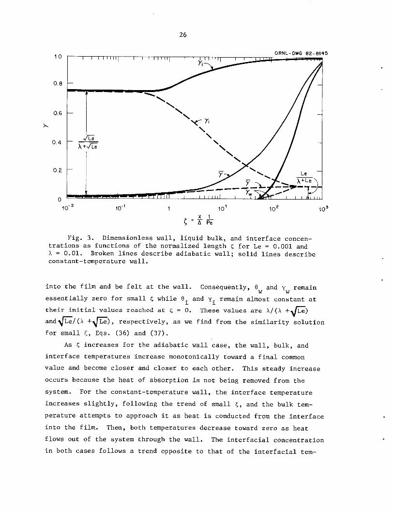
Figures 4 and 5 describe typical temperature and concentration
profiles across the film for typical values of z,. At small z, the
gradients of both quantities are very sharp and their variations are
P~
77 ' 'I
1 h \0.8
KLYo.o, L—
0.6 7 1 —
0.4
---10
--100
0.2
n n 1 1 1 1 1 1 I I
—
0.0 0.2 0.4 0.6
9
0.8
P-
ORNL-DWG 82-8149R
r$J^^O.01I I I
0.8r—o.i
—
1"~~10
—
0.6 I— 100—
0.4 j —
0.2 —
n n I I I I I I I I
0.2 0.4 0.6
7
0.8 1.0
Fig. 4. Typical profiles of dimensionless temperature and concentration across the film at different values of z, for adiabatic wall
where Le = 0.001 and A = 0.01.
p-
0.0 0.2 0.4 0.6
9
0.8
28
ORNL-DWG 82-8147R
Fig. 5. Typical profiles of dimensionless temperature and concentration across the film at different values of Z, for constant-temperaturewall where Le = 0.001 and A = 0.01.
limited to a thin layer near the interface. As z, increases, the effects
at the interface diffuse toward the wall and the gradients become more
moderate. There are, in fact, two boundary layers, one of temperature
and one of concentration, which develop starting from the point of dis
continuity (z, = 0, n = 1) . The former develops considerably faster than
the latter, as the thermal diffusivity a is larger than the mass diffusion
coefficient D.
The effect of the heat of absorption A is illustrated in Figs. 6
and 7, describing the temperature and concentration at the interface and
at the wall, respectively. In the former, each curve represents either
0. or y- when read on the corresponding scale, since 0. + y. - 1. The
initial value (z, = 0) of the interface temperature increases with A,
and that of the interface concentration decreases, according to the
formulas shown in Figs. 2 and 3. The same is true for the asymptotic
values of temperature and concentration, respectively, both at the
interface and at the wall. The heat of absorption A does not seem to
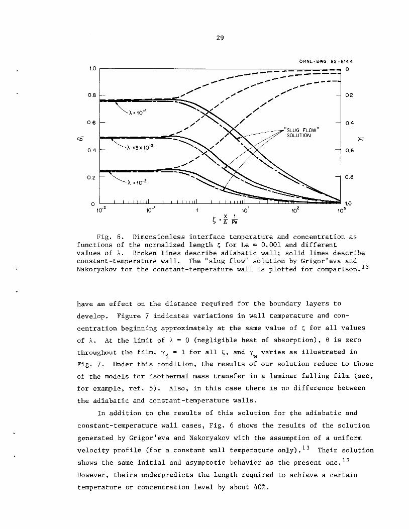
29
1.0
CD
ORNL-DWG 82-8144
0
- 0.2
0.4
>T
0.6
0.8
Fig. 6. Dimensionless interface temperature and concentration asfunctions of the normalized length z, for Le = 0.001 and differentvalues of A. Broken lines describe adiabatic wall; solid lines describe
constant-temperature wall. The "slug flow" solution by Grigor'eva andNakoryakov for the constant-temperature wall is plotted for comparison. 13
have an effect on the distance required for the boundary layers to
develop. Figure 7 indicates variations in wall temperature and con
centration beginning approximately at the same value of z, for all values
of A. At the limit of A = 0 (negligible heat of absorption), 0 is zero
throughout the film, Y- = 1 f°r aH £j ancl Y varies as illustrated ini w
Fig. 7. Under this condition, the results of our solution reduce to those
of the models for isothermal mass transfer in a laminar falling film (see,
for example, ref. 5). Also, in this case there is no difference between
the adiabatic and constant-temperature walls.
In addition to the results of this solution for the adiabatic and
constant-temperature wall cases, Fig. 6 shows the results of the solution
generated by Grigor'eva and Nakoryakov with the assumption of a uniform
velocity profile (for a constant wall temperature only).13 Their solution
shows the same initial and asymptotic behavior as the present one.13
However, theirs underpredicts the length required to achieve a certain
temperature or concentration level by about 40%.
$CD
1.0
0.8 -
0.6 -
0.4 —
0.2
-210'
30
"I I I TTTT| | I I I I I I l| I I I I I I I I | f
J£.J I i L
10"
\ i i i i ml i i i i i ml i l
r =211.b A Pe
101
ORNL-DWG 82-8157
10' 10°
Fig. 7. Dimensionless wall temperature and concentration as functionsof the normalized length z, for Le = 0.001 and different values of A.Broken lines describe adiabatic wall; solid lines describe constant-
temperature wall.
The effect of the Lewis number is shown in Figs. 8 and 9, describing
the temperature and concentration at the interface and at the wall,
respectively. As in Fig. 6, each curve in Fig. 8 represents either 0.
or y.. The initial and asymptotic behaviors are as predicted by the
formulas given in Figs. 2 and 3. An increase in Le leads to a decrease
in 0. and to an increase in y •> at z, = 0 for both cases and at Z -> °° fori i
the adiabatic wall case. In addition, Le has an effect on the develop
ment of the concentration boundary layer. The larger Le, the shorter
the distance required for the concentration change to reach the wall, as
shown by the curves for y in Fig. 9.w
Figure 10 shows the mass flux at the interface, y., as a function
of t, for Le = 0.001 and different values of A. Under all conditions,
the rate of absorption is lower for an adiabatic wall than for a
constant-temperature wall. Initially, at small z,, the curves for the
two cases coincide. For larger Z,, after the thermal boundary layer has
become fully developed, the heat removed at the wall enhances the mass
1.0
0.8
0.6
CD
0.4 -
02 ~
10"
31
ORNL-DWG 82-8151
0rrn i i i i i m ii i i i I i 1111 i i i i 11 n3^^
-Le=10"
-Le =10"
— Le=10"'imI i i i iinil
10" 10'
i 4 Pe
- 02
0.4
X-
0.6
0.8
1.0
10' 10°
Fig. 8. Dimensionless interface temperature and concentration asfunctions of the normalized length z, for A = 0.01 and different valuesof Le. Broken lines describe adiabatic wall; solid lines describe constant-
temperature wall.
1.0ORNL-DWG 82-8154
i—i i i 111 1—i i mmi r
0.8
0.6
>?
CD
0.4
0.2
J L_L U^10 10 10 10 10
^ A Pe
Fig. 9. Dimensionless wall temperature and concentration as functionsof the normalized length z, for A = 0.01 and different values of Le.Broken lines describe adiabatic wall; solid lines describe constant-
temperature wall.
32
120ORNL-DWG 82-8153
100 —
Q - A Pe
Fig. 10. Dimensionless mass flux at the interface as a function ofthe normalized length Z, for Le = 0.001 and different values of A.Broken lines describe adiabatic wall; solid lines describe constant-temperature wall.
transfer in the constant-temperature wall case. The point at which the
solid and broken curves part may serve as a measure for the length
required for the full development of the thermal boundary layer. The
value of y. tends to zero at large z, for both cases. Also, increasing
A reduces the mass flux, as expected. The curve for A = 0 describes the
case of isothermal mass transfer, in which y. is the largest possible
value for the given Le, and where there is no difference between the
adiabatic and constant-temperature walls.
6. HEAT AND MASS TRANSFER COEFFICIENTS
The literature is often somewhat ambiguous about the definition of
heat and mass transfer coefficients. This is particularly so in problems
of simultaneous heat and mass transfer due to the coupling between the
two processes. Yih and Seagrave have used two different definitions of
the Sherwood number, one based on (C. - C) and the other on (C. - C ).^1 1 o
Nakoryakov and Grigor'eva have defined it based on (C - C ).11+ Tamir
and Taitel have used an additional definition of an average Sherwood (or
Nusselt) number based on a logarithmic mean concentration (or temperature)
difference.5
We will define the transfer coefficients based on the quantity
difference which constitutes the driving force for the transfer phe
nomenon. The coefficient of local mass transfer from the interface to
the bulk of the liquid is defined through the Sherwood number as
Sh =-£- =7 ^=r . (38)D (Y± " T)
The coefficient of local heat transfer from the interface to the bulk of
the liquid is defined through the Nusselt number as
hTA y A
In the constant-temperature wall case we must also consider the heat
transfer coefficient from the bulk of the fluid to the wall. Hence,
Nu' =
h-x/A qT = Jw . (40)
Figure 11 describes the Sherwood number as a function of the
normalized length z, for different values of Le and A. The value of Sh
is very large for small Z, and decreases toward an asymptotic value as z,
increases. For each set of conditions, Sh is greater for a constant-
temperature wall than for an adiabatic wall. The reasons are the same
as those for y. (Fig. 10). The behavior in the two cases is the same
33
10° I I I I I l| 1 TT
10 —
10
J I I I II III J I I I M i il
10"' 10"
34
ORNL-DWG 82-8156
"I I I II I ll| "1 1 I I M !l| "1 1 I I I 114-1
X=io-'\Le =10"-5X
<-, " A Pe
X=10"2 .Le=10l->^
I I I iVll I I I I llfrj
101 10'
3.45 -
J l_± J_LL
10*
Fig. 11. Local Sherwood number as a function of the normalized
length z, for different values of Le and A. Broken lines describeadiabatic wall; solid lines describe constant-temperature wall.
for small t,, and the discrepancy begins when the thermal boundary layer
has reached the wall, increasing with Z,.
In the case of a constant-temperature wall, the effect of A on Sh
is small. For fixed A, Sh is larger for smaller Le, contrary to what
may be expected, because while the mass flux y. increases with Le, the
driving force (y. - y) increases even faster. A smaller Lewis number
requires a larger distance for the concentration boundary layer to
become fully developed. For all combinations of A and Le, the Sherwood
number for a constant-temperature wall tends to an asymptotic value of 3.45.
In the case of the adiabatic wall, increasing A reduces Sh signifi
cantly for all values of Le. A larger A leads to a greater deviation
from the constant-temperature wall behavior, this deviation shrinking to
zero for A = 0. For fixed A, a larger Lewis number results in a smaller
deviation. Unlike the constant-temperature wall case, the asymptotic
value of Sh depends on A and Le, decreasing with the former and increasing
with the latter.
35
The variations of Nu and Nu' with Z, are illustrated in Fig. 12 and are
considerably less marked than that of Sh. In the initial region of de-
10:"I 1—I I I I I II
10'
10
J L I I II
10" 10"
~1 1—I I I I III \ I I I I
J I I I I I I II
iA _!_A Pe
101
ORNL-DWG 82-8152
~1—I I MM] 1 1 I I I I11
4.23
2.65
J It _|JU1.60i i i i
10' 10J
Fig. 12. Local Nusselt number as a function of the normalizedlength z,. The curves are almost unaffected by variation in Le between10~^ and 10~2 and by variations in A between 10~3 and 10-1. Brokenlines describe adiabatic wall; solid lines describe constant-
temperature wall.
velopment of the thermal boundary layer, Nu decreases in the same manner
for the adiabatic and for the constant-temperature wall cases. In this
region, Nu' is zero, as the effects at the interface have not reached
the wall. Beyond that region there is little variation in Nu, which
tends to the asymptotic values of 4.23 and 2.65 for the adiabatic and
constant-temperature wall, respectively. The asymptotic value of Nu'
reaches 1.60. This behavior is almost unaffected by A and Le for a wide
range of values of these parameters.
The results of the "slug flow" model by Grigor'eva and Nakoryakov
show the same general behavior, but the actual values of the coefficients
deviate by about 20% from those of the present analysis.13 With theassumption of a uniform velocity profile and a constant-temperature wall,
the asymptotic value of Sh is 3.00, and that of both Nu and Nu' is 2.00.

7. INTEGRAL SOLUTION
In addition to the exact solutions described in the previous sec
tions, an approximate integral method was employed, and its results were
compared with those of the former. The advantage of the integral method
is its simplicity and the possibility of obtaining explicit formulas for
most of the parameters of interest. Computing time was reduced signifi
cantly and the results agreed very well with the exact solutions.
The mathematical formulation of the integral solution and its results
are described in this section. Readers uninterested in these details
should skip to Sect. 8.
7.1 Formulation
The integral method of solution converts the partial differential
Eqs. (7) and (8) into ordinary ones by assuming the shape of the tem
perature and concentration profiles across the thin liquid film, based
on the given boundary conditions. The exact shape of those profiles is
not our primary interest; rather, it is important to learn about the
variation with z, of the temperature and concentration at the interface
and at the wall, from which the heat and mass transfer coefficients can
be calculated. When the profiles assumed satisfy the boundary conditions
and are close in shape to the actual ones, the integral method gives
results close to those of an exact solution, as has been demonstrated in
many boundary layer problems as well as in a case similar to the present
one of isothermal mass transfer in a falling film.
The integral form of Eqs. (7) and (8) is obtained by integration
across the film thickness and making use of the conditions (9a-c) and
(lOa-c). Energy Eq. (7) becomes
oT / vS dT1 =V " % > (41)
where q is the dimensionless heat flux at the wall, q = [39/3nJ„_n*nw w ti-u
The diffusion equation, Eq. (8), becomes
/'
37
d_
d5 r vy dn = Ley.
38
(42)
Before proceeding with the formulation of temperature and concentration
profiles, it would be useful to consider their qualitative behavior.
Figure 13 describes the variations in concentration and temperature for
ORNL-DWG 84-4737R
""m
e
•^-
ITHERMAL
BOUNDARY
LAYER
DEVELOPING \N
>9
r$THERMAL
BOUNDARY
LAYER FULLY., ,DEVELOPED \V
jCO
-V-
(a)
^
7n
^<
-V-I I 11 I I
CONCENTRATIONBOUNDARYLAYER
DEVELOPING
£<
CONCENTRATIONBOUNDARY
LAYER FULLY
DEVELOPED
I(b)
Fig. 13. Qualitative distribution of the temperature and concentration in the falling film: (a) adiabatic wall and (b) constant-temperature wall.
35
the two cases of interest — the constant-temperature wall and the adiabatic
wall. The liquid at Z, = 0 is at a state of nonequilibrium with the
vapor. As a result, a process of simultaneous heat and mass transfer begins
at the interface and extends its effect gradually into the film. Thermal
and concentration boundary layers begin to develop and grow in thickness
until they fill the entire depth of the film. As will be shown later,
the thermal boundary layer usually becomes fully developed first.
For both layers in this developing region, the temperatures and
concentrations at the interface are functions of the boundary layer
thickness, which is itself a function of z,. Once fully developed, the
profiles continue to vary over the entire film thickness as long as the
transfer process at the interface continues. After sufficient distance
in the direction of flow, the temperature and concentration become
uniform across the film as equilibrium is reached.
In accordance with the above, let us denote the value of z, where
the thermal and concentration boundary layers become fully developed by
z, and Z, , respectively. We will assume the following profiles, satisfying
the boundary conditions (9b) and (9c):
1. Concentration.
In the developing boundary layer region, 0 <_ z, <_ z, ,
(o for 0<n<(1 - «)Y = , («a)
|Y. [(1 - Sy - n)/<Sy]2 for (1 - 6y) <t, <1
which also satisfies y = 0 and 3y/3h = 0 at the edge of the boundary
layer. The bulk concentration in this region would then be
y=X VY dri =T(\ "lo-/ (43b)In the fully developed boundary layer region, z, >_ z, ,
Y = YTT + (Y, " Y )n2 , (*4a)w l w
40
where y is the dimensionless concentration at the wall. The bulk con-w
centration for this region becomes
Q vY dn =|q (9y± +HYW) • (44b)
Note that at the point of transition between the two regions, C = C ,
where 6=1 and y = 0, we obtain y = y.12 and y = 9y./20 from bothY w 11
Eqs. (43a-b) and (44a-b).
2. Temperature.
In the developing boundary layer region, 0 j< x, <_ t, ,
0 for 0 < n £ (1 - 6 )
(45a)
ei [(1 - <5Q - n)/6Q]2 for (1 - SQ) <n<1
with the bulk temperature
0= j0 v6 dn = ^ -§-J. (45b)The same profiles apply in this region to both the adiabatic and constant-
temperature wall cases.
In the fully developed boundary layer region, t, > z, ,6
then for the adiabatic wall,
6=0 + (6. - 0 )nz , (46a)w 1 w
0=^ (90. +110w) , (46b)
where 0 is the dimensionless temperature at the wall. For the constant-
temperature wall,
V + (9i - qw)n ' (46c)
h (18ei +V ♦ (46d)
41
where q is the dimensionless heat flux at the wall.
Note that at the point of transition between the two regions, z, = z, ,
where 6=1 and 0 = 0 or q =0 (for the adiabatic and constant-w w
temperature wall, respectively), we obtain 0 = 0.n and 0 = 90./20 from
both Eqs. (45a-b) and (46a-d).
Substitution of the above profiles in the integral Eqs. (41) and
(42) yields
(1) Energy equation:
r \50" To-/
•^k (90. + 116 ) = y.A for adiabatic wall,20 l w J l
~r (180. + 7q ) = y.A - q40 l w J x w
= y.A for 0 < z, < Z, ;l o
(47a)
(47b)
or
d_dC
d?
d_d?
for Z, >_ ?Q .
(2) Diffusion equation:
6 3'
for constant-tem
perature wall,
d_d?
d_d? h (9Yi +llYw}] =Leyi for c S
= Ley. for 0 < z, < z, ,l — — y
Also, from Eq. (10b) and the concentration profile,
u. = 2y./<5 for 0 < C < X, ,l i Y — Y
y, = 2(y. - Y ) for ? > c ,l l w y
and from Eq. (10c) and the temperature profile,
y A = 29/6. for 0 < ? < Z, ;1 ID — — O
y.A = 2(0. - 0 ) for Z, > Z,a, adiabatic wall ;l l w — o
y.A = 20. - q for z, > z,n, constant-temperature walll l w — 0
(47c)
(48a)
(48b)
(49a)
(49b)
(50a)
(50b)
(50c)
42
Equations (47a-c) and (50a-c) plus the equilibrium condition at the
interface (10a) provide five equations for the five unknown variables of
interest: 0., y., y., 6 alternating with y , and 6. alternating withl l l y w 0
0 for the adiabatic wall or with q for the constant-temperature wall.w w
All are functions of the single independent variable z,. The variable A
may be expressed in terms of 0. and Y- at each point. The boundary
conditions are
6„ = 0 and 6=0 at z, = 0 , (51a)0 Y
for the developing boundary layer regions, and
Yw = 0 at ?= ^ where 5=1; (51b)
0=0 for adiabatic wall,w
or > at z, = z, where 6. = 1 ;o o
(51c)
for the fully developed regions.
7.2 Solution
Figure 13 describes three zones of the liquid film, indicated by
numerals 1, 2, and 3. In zone 1 both the thermal and concentration
boundary layers are developing, in zone 2 one is fully developed and
the other still developing, and in zone 3 both boundary layers are
fully developed. Our solution will proceed from one zone to the next
in that order.
Zone 1
As is evident from Fig. 13, the behavior in this zone is the same
for both the adiabatic and constant temperature wall cases. The equations
in effect are (47a), (48a), (49a), (50a), and (17a), with the boundary
43
condition (51a). Eliminating y. between Eqs. (47a) and (48a), integrating
the resulting differential equation, and applying the boundary condition
yields
Y- o, U„ -t£- I- v.. Is.. -t*- I • (52)'i (*e -¥)-*i (\"£)Eliminating y. between Eqs. (49a) and (50a) gives
Y. , 0.
r-Tt- (53)Y
Combining Eqs. (52) and (53) results in
(>-*)-v(>-#)Lefi„2 1 - ^ = 6 2 i - -JL. I. (54)
Since 6 and 6. are both less than or equal to unity, it is clearY 0 j,
from Eq. (54) that the ratio 6 /6 is of the order Le2. For most ab
sorbent liquids the Lewis number is much smaller than one. It is there
fore evident that the thermal boundary layer becomes fully developed
when the concentration boundary layer is still quite thin. We thus
find, from Eq. (54),
6 =Y V^'ef-B") • (55)
and in particular, 6 =^9Le/10 at z, = CQ where 6Q = 1. By substituting6 from Eq. (55) into Eq. (53), and making use of Eq, (17a), we canY
express 0. and y. in terms of 6 :
1 +
(56a)
v = > . (56b)i
44
The bulk temperature and concentration from Eqs. (45b) and (43b) become
(56c)
- 1Y = T
*e I1-if)
LA1+vnf1.v)'5
A \ 10 /
(56d)
Now all the quantities of interest have been expressed in terms of
6 ; it remains to determine how 6 varies with z,O
a Eq. (50a) into Eq. (47a) and 0. from Eq. (5
equation, we obtain the following differential equation
By substituting y.A
from Eq. (50a) into Eq. (47a) and 0. from Eq. (56a) into the resulting
d_d?
(s-tf)l>•-¥(• -£)"J ...•<¥(.-£)''
which may be integrated, using boundary condition (51a) to deter
mine the constant of integration. Since 6 <_ 1, the resulting ex
pression may be given a somewhat simplified approximate form, by ex
panding in terms of the small quantity (6 2/10) and neglecting high
powers of it:
81 -
10
(l + (3/2)A/Le\\ 1 + A/Le /
The point where the thermal boundary layer becomes fully developed is
found by substituting 6=1 into Eq. (58a):
Ke so1 + (17/18)A/Le
1 + A/Le
(57)
(58a)
(58b)
45
Zone 2
Although in zone 1 the behavior was the same for the adiabatic and
the constant-temperature wall, here a distinction must be made between
them.
Adiabatic wall. The equations in effect are (47b), (48a), (49a),
(50b), and (17a), with the boundary condition (51c). Eliminating y.
between Eqs. (47b) and (48a), integrating the resulting differential
equation, and applying the boundary condition, yields
^ (90. + 110 )^-10 l w A (v^-H
Eliminating y. between Eqs. (49a) and (50b) gives
3 ) = x Tw 6
Eliminating 0 between Eqs. (59) and (60) provides a relation betweenw
0., Y-> and 6 which, together with Eq. (17a), yields
Yi
11 +_L10 Le26
Y \- (• -*)]1 +
1 +
10 Le V 1026Y L
26Y L
H + -X.10 Le
(• -*)]'
(-*The term 0 can now be found from Eq. (60)
w
26Y L
10 Le I 10K)]w
1 +26
Y "-10 Le (• •m
(59)
(60)
(61a)
(61b)
(61c)
46
The bulk temperature and concentration from Eqs. (46B) and (43b) become
Y U32Le
11 +_Y_10 Le1 + 26
\ (* -£)(• •m
- 1
1 +26
11 +10 Le
6 2Y (• -*)]
(61d)
(61e)
All the quantities of interest have now been expressed in terms of
6 . To find the variation of 6 with £, we substitute y.A fromY Y . i
Eq. (50b) in Eq. (47b) and 0. and 0 from Eqs. (61a) and (61c) in the1 w
resulting equation:
(*-£)d_d?
6 + jY 2
11 +_X10 Le (• -m
= 4Le
6 +\Y 2
1
10 Le \ --)110 /J
which may be rewritten as
n 6 210 Le
d6__L
4Le
(62a)
= dC (62b)
47
Equation (62b) may be integrated numerically as 6 varies from y9Le/10to 1, and z, varies correspondingly from z, to z, . An adaptive quadra
ture method was used in the above integration.18
Constant temperature wall. The equations in effect are (47c),
(48a), (49a), (50c), and (17a), with the boundary condition (51c). Elim
ination of y. and 0. from Eqs. (49a), (50c), and (17a) provides an
expression for qw
i =2fi -y. -*rjT 1•w V x \)q = 2 fl - y. - *tM • (63)
Substitution of y.A from Eq. (50c), q from Eq. (63), and 0. from
Eq. (17a) into Eq. (47c) gives
d (16y. + 7X-^- )= 40 (1 - y. - 2A -± ) d? . (64)V x \/ V x 6y/
Also, substitution of y. from Eq. (49a) into Eq. (48a) yieldsl
h (** -^). 4Le t^ dr, , (65)o
Y
and elimination of t, between Eqs. (64) and (65) results in a differential
equation relating y. to 6 :
1[l6Tl +7A (T./6y)] ^ d[Y± (fi, -6^/10)]Le (y±/6y)
which may be rewritten as
dY. Y± 7A - (10/Le)(6Y + 2A - Sy/y.) (1 - 36^/10)6^d6 6 (7A + 166 ) + (10/Le)(6 + 2A - 6 /y.)U - 6 2/10)6 2YY Y Y Y i Y Y
(66a)
(66b)
48
Equation (66a) may be integrated with the boundary condition originating
from (56b):
v^EL_ ats -V5w^. (67)A + "^ 9Le/10 Y
where z, = z, . Once y. has been found in terms of 6 , 0. and q may be0 i y l w
expressed in terms of 6 by means of Eqs. (17a) and (63). The bulk
temperature and concentration 0 and y may be determined from Eqs. (46d)
and (43b), respectively. It remains to determine how 6 varies with z.Y
An equation relating these two may be obtained by combining Eqs. (65)
and (66b):
Ar -, 7A6 (1 - 6 2/5) + 86 2(1 - 36 2/10)Q.Z, _ 1 y_ y y y '
d6 2 (7A + 166 )Le + 106 2(6 + 2A - 6 /y.)(l - 6 2/10)Y Y Y Y Y i Y
(68)
Equations (66b) and (68) were integrated simultaneously using a fourth-
order Runge-Kutta method.18 The value of X where 6 becomes equal toY
unity marks the end of zone 2.
Zone 3
In this zone both boundary layers are fully developed. Again, a
distinction must be made between the adiabatic and constant-temperature
wall cases.
Adiabatic wall. The equations in effect are (47b), (48b), (49b),
(50b), and (17a), with the boundary condition (51c). Eliminating y.
between Eqs. (47b) and (48b), integrating the resulting equation, and
applying the boundary condition, yields
("i +119w) =t (9Yi +UV • (69)
Eliminating y. between Eqs. (49b) and (50b) gives
(0. - 0w) = A(y. - yw) . (70)
49
Equations (69), (70), and (17a) may be combined to express y., 0., and
0 in terms of y as follows:w w
1 - (11/20)(A/Le)ywYi =1+ (9/20)(A/Le) ' (71a)
A (9/20) + (ll/20)y
Le 1 + (9/20)(A/Le)* , (71b)
1 - Yw " (*/Le)Yw3w = 9i " Xl + (9/20)(A/Le) ' (71c)
Here, terms of the order Le have been neglected with respect to unity.
Note that 0. and 0 are very close to each other; the difference between1 w
them is of relative order Le. The bulk temperature and concentration
from Eqs. (46b) and (44b) become
. (9/20) + (11/20)y + (11/20)Ay
H ~ Le 1 + (9/20)(A/Le) ' W '
(9/20) + (ll/20)y + (ll/20)Ay— _ W W (lla'\Y " 1 + (9/20)(A/Le) ' U J
Now all the quantities of interest have been expressed in terms of
the dimensionless concentration at the wall, y . It remains to findw
how y varies with z,. Substituting y. from Eq. (49b) into Eq. (48b) andw i
y. from Eq. (71a) into the resulting equation yields
J, [lo+i(1 +X)Yw] -2Le[l-Yw- Le Yw
which may be integrated with the boundary conditions (51c) to give
Yw
/ Le_\ L T 40 /he + a\"\iTTT j [l ~exp [- U\^TTJ (c - v
Constant temperature wall. The equations in effect are (47c),
(48b), (49b), (50c), and (17a), with the boundary condition (51c).
(72)
(73)
50
Eliminating u± and B± between Eqs. (49b), (50c), and (17a) provides anexpression for q :
w
qw " 2[1 + % " (1 + A)Yi] ' (74)
Substitution of y±A from Eq. (50c), q from Eq. (74), and 0. fromEq. (17a) into Eq. (47c) gives
(16 + 7A)dy± - 7Adyw =40[(1 -y±) + 2A(yw - Y±)]d . (75)
Also, substitution of y. from Eq. (49b) into Eq. (48b) yields
9dYi + lldyw = 40Le(Y. - Yw)d? . (76)
Eliminating dz, between Eqs. (75) and (76) results in a differential
equation relating y. to y :i w
(16 + 7A)dy. - 7Ady 9dy. + lldyi w 1 'w
(1 - y ) + 2A(y - y.) Le(y. - y ) 'i w 1 1 w
(77)
which may be integrated with the boundary condition at ? = ? (whereY
Y = 0 and y = y * as obtained from the solution for zone 2), yielding
(1 - y ) - 2A(y - y )i 1 w
(1 - y.') - 2AYi'I"! -(»!,, +llV/20l (iij±^)
1-9yi'/20 J ' (78)
The term in the brackets on the right-hand side of Eq. (78) is also equal
to (1 - y)/(l - y'). It is a number smaller than unity, taken to a very
large power due to Le « 1. It can be shown that this results in
1 - Y± - 2A(y. - yw) = 0(Le) - 0 ; (79a)hence,
Y± = (1 + 2Ayw)/(l + 2A) ; (79b)from Eq. (17a),
0. = 2A(1 - yw)/(l + 2A) ; (79c)
51
from Eq. (74),
q = 2A(1 - y )/(l + 2A) . (79d)w w
The bulk temperature and concentration, 0 and y, may be determined
from Eqs. (46d) and (44b), respectively:
0 = (5/4)A(l - y )/(l + 2A) ; (79e)w
y = (1/20)(9 + lly + 40Ay )/(l + 2A) . (79f)w w
It remains to determine how y varies with X,. Substituting y. fromw 1
Eq. (79b) into Eq. (76) yields
^ 40 Le d? , (80)(1 - y ) (11 + 40A)
w
which may be integrated with the boundary condition (51b) to give
|_ yn + 40Ayyw= 1 - exp -(11 + 40AJLe(^ " V (81)
7.3 Results
Figure 14 describes the main system's parameters as they vary
through the three different zones for a typical set of values of Le and
A. The dimensionless boundary layer thickness, temperature, concen
tration, and heat and mass flux are shown as functions of the normalized
length C. Due to the largely different lengths of the three zones, a
logarithmic scale has been chosen for z,, with a small linear portion
near the inlet end. As in the results of the exact solutions, the
solid lines describe the results for the constant temperature wall and
the broken lines for the adiabatic wall case.
In zone 1, the behavior is the same for the adiabatic and constant-
temperature wall cases. The thermal boundary layer develops from zero
to its full thickness while the concentration boundary layer develops
partially to a normalized thickness \ 9Le/10 at the end of the zone.
The interface temperature and concentration are essentially constant at
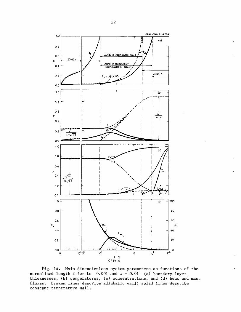
0.0
1.0
0.8 -
0.6 -
0.4 -
0.2
x*yue
1.0
0.8
1__
0.6
04 - yr
X*yEe
0 2
52
ORNL-DWG 81-4734
I I lit
I \s •
(b) "
!
i A ii ,-' !1 ' i i
i y X
i *♦* i i X*Le
- ! .'/ i i- I S/'Sy j j
^U**^ s ^"""•^^^'^^-^-"^i9"-' ^""" ^^ i 1 I
_
I
I I
—r
i(0 ^
I
•~^£k II
"<
\
\ |\
\ I
_>l/
/ lrm
J Le -
- 100
\i i :
id)
- \,K
I
-
«»i
i i nu ' I MINI I I TtHJlJ 1_Lep
I
80
60
40
20
-2 -210 10 10 10 10 10"
C=Pe A
Fig. 14. Main dimensionless system parameters as functions of thenormalized length X, for Le 0.001 and A = 0.01: (a) boundary layerthicknesses, (b) temperatures, (c) concentrations, and (d) heat and massfluxes. Broken lines describe adiabatic wall; solid lines describe
constant-temperature wall.
53
the value reached initially at X, = 0 upon contact with the vapor
[A/(A + "^Le) and Le/(A +yjhe), respectively]. The wall temperatureand concentration are zero. The bulk temperature and concentration are
close to zero and increasing. There is no heat flux through the wall;
however, the mass flux y. in this zone is quite high, as the driving
force for mass transfer is at its maximum. The length of zone 1 is
given by Eq. (58b). It is almost constant at X, = 9/80, decreasing
slightly with A/-yLe.
In zone 2 the concentration boundary layer reaches its full thickness,
becoming fully developed after a shorter distance from the inlet in the
adiabatic than in the constant-temperature wall case. In the former
case, the wall, bulk, and interface temperatures increase monotonically
toward a final common value and become close to each other at the end of
the zone. This steady increase occurs because the heat of absorption is
not being removed. For the constant-temperature wall, the interface and
bulk temperatures increase slightly, following the trend of zone 1, then
decrease toward zero as heat flows out of the system.
The heat flux q in this case begins at zero value at z, = X, , in-w W
creases and reaches a maximum as more heat of absorption is created, and
then decreases toward zero and has a low value of 2A/(1 + 2A) at the end
of the zone. The interfacial concentration in both cases follows a
trend opposite to that of the interfacial temperature, since y^ = 1 - 0.^
[Eq. (17a)]. The bulk concentration increases in both cases toward a
final value equal to that of y..
In zone 3 both boundary layers are fully developed. External heat
and mass fluxes are small and changes in the temperature and concentration
profiles take place by virtue of thermal and mass diffusion within the
film, tending to make those profiles uniform. The temperature and con
centration tend toward an asymptotic value, which may be found by
substituting z, -> <=° in the results of the solution for zone 3. In the
constant-temperature wall case, the dimensionless temperature becomes
equal to that of the wall (0=0) and the concentration reaches the
corresponding equilibrium value (y = 1). In the adiabatic wall case the
asymptotic temperature reflects some increase from the initial value
[0 = A/(Le + A)], and the corresponding equilibrium concentration
54
[y = Le/(A + Le)] is lower than the thermodynamically possible value of 1.
The results of the integral solution were found to be in very good
agreement with those of the exact solutions described earlier.
8. NUMERICAL EXAMPLE
The following example will illustrate the use of the results ob
tained earlier for calculating the parameters in a practical case.
Consider a film of LiBr-H„0 solution flowing down over a tray inclined
at 45°, at a mass flow rate of 0.25 kg/s per meter of breadth. The
initial temperature and concentration of the solution are 75°C and 60%
LiBr by weight, respectively. The film is in contact with dry saturated
water vapor at 45°C which has a vapor pressure higher than that of the
solution at the above conditions and is therefore being absorbed. We
would like to calculate (1) the maximum change in solution concentration
achievable when the tray is adiabatic, (2) the same when the tray is
being cooled from below and kept at a constant temperature, (3) the
maximum temperature rise of the solution in the adiabatic case, and
(4) the length of tray required, in the direction of flow, to produce
90% of the maximum concentration change in either case.
The absorption process is described on a thermodynamic equilibrium
chart (taken from ref. 19) in Fig. 15 for both the adiabatic and constant-
temperature cases. The solution at its initial state has a vapor pressure
of 4.8 kPa, considerably lower than that of the vapor at 45°C (9.7 kPa).
In the case of the adiabatic wall, the water concentration in the absorbent
increases (LiBr decreases) and the bulk temperature increases. For the
constant-temperature wall, the bulk temperature is the same at the
beginning and end of the process; however, in between there is some
increase in temperature, as illustrated in Fig. 2.
We will begin by calculating the flow velocity and film thickness.
The physical properties of LiBr-H„0 solution under the present temperature
and concentration are listed in Table 2. The film Reynolds number is
given by ref. 1:
Re = 4l7y = 4 X °'" = 333 .3 x 10
The flow is, therefore, clearly laminar (Re < 500). Then, from the
Nusselt formula for falling films:1
55
M ' I 'I ' I ' I ' I
ADIABATIC WALL
CONSTANT
TEMPERATURE
WALL
56
ORNL-DWG 82-8155
200
150
100
50
40
30
20
10
54
3
2
1
0
Ixl<rz>COCOLUeco.
cr
oO-
COm<
120
110
100<>o
W90
=>
$ 80oruia.
> 70iiiH
rr 60on
5 50
hi
fcr 40mrrocom
30<
20
10
0
10 20 30 40 50 60 70 80 90 100 110 120 130 140 150 160 170
SOLUTION TEMPERATURE. °C
180
Fig. 15. Thermodynamic equilibrium chart for LiBr-H„0 solution,taken from ref. 19, illustrating the absorption process with an adiabaticwall and a constant-temperature wall, under the conditions of thenumerical example.
A =/ 3yr \i/3. /\p2g sin $ J \
3 x 3.0 x 10 x 0.25
(1.72 x 10³)2 x 9.8 sin 45' )'/3
= 0.48 x 10⁻³
m
0.25u =
pA 1.72 x 103 x 0.48 x 10"3= 0.30 m/s
Next, we find the equilibrium concentration and temperature C and
T used to calculate the normalized quantities y and
definition, we find from the diagram, Fig. 15:
Based on this
kmole HO
C = 52.8% LiBr = 47.2% Ho0 = 45.1e 2 3 . ^.
ip. solution
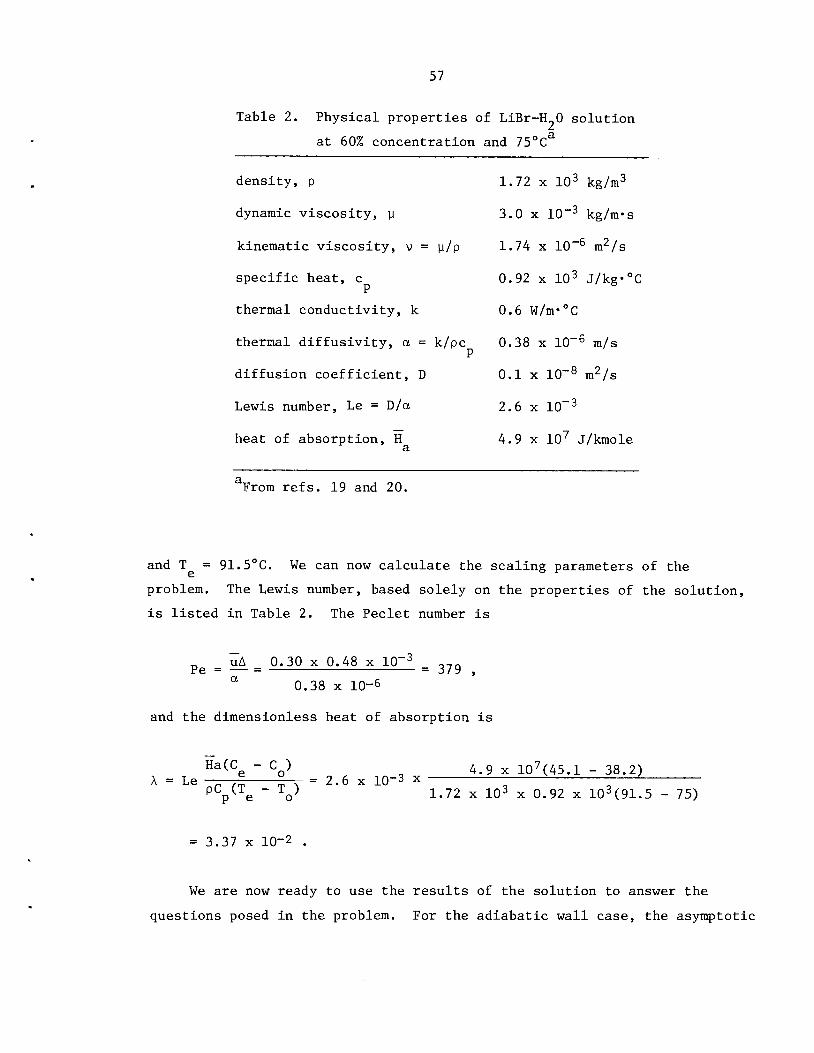
57
Table 2. Physical properties of LiBr-H_0 solution
at 60% concentration and 75°C
density, p 1.72 x 10³ kg/m3
dynamic viscosity, y 3.0 x 10"3 kg/m-s
kinematic viscosity, v = y/p 1.74 x 10⁻⁶ m2/s
specific heat, c 0.92 x 10³ J/kg«°C
thermal conductivity, k 0.6 W/m*°C
thermal diffusivity, a = k/pc 0.38 x 10⁻⁶ m/s
diffusion coefficient, D 0.1 x 10⁻⁸ m2/s
Lewis number, Le = D/a 2.6 x 10"3
heat of absorption, H 4.9 x 10⁷ J/kmole
aFrom refs. 19 and 20.
and T = 91.5°C. We can now calculate the scaling parameters of the
problem. The Lewis number, based solely on the properties of the solution,
is listed in Table 2. The Peclet number is
uA 0.30 x 0.48 x 10~3 „,„Pe = — = = 379 ,
a 0.38 x 10⁻⁶
and the dimensionless heat of absorption is
Ha(Ce " Co) „ 4.9 x 10⁷(45.1 - 38.2)A=Le —-t| 5-y = 2.6 x 10"3 x '-pCp(Te - Tq) 1#72 x 103 x 0.92 x 103(91.5 - 75)
= 3.37 x 10"2 .
We are now ready to use the results of the solution to answer the
questions posed in the problem. For the adiabatic wall case, the asymptotic
58
values of the normalized temperature and concentration, 0 and y, were
found to be A/(A + Le) and Le/(A + Le), respectively. Thus,
A 3.37 xlO"2 =0.928 =Ta3_T°°° A + Le -9 a T-T'
Le 3.37 x 10 2 + 2.6 x 10"3 e o
T, = 75 + 0.928(91.5 - 75) = 90.3°C ,
- Le 2.6 x 10~3 Coo ~ C0Y~ =tt^ = : =°-0716 - -c—^-f3.37 x 10"2 + 2.6 x 10⁻³ °e o
Cm = 38.2 + 0.0716(45.1 - 38.2) = 38.7 kmole H20 per m3 solution
= 59.5% LiBr .
It is thus found that in adiabatic absorption the temperature of
the solution increases from 75 to 90.3°C, almost as high as the no-mass-
transfer limit of 91.5°C. The concentration change is small, only from
60% LiBr to 59.5% LiBr. However, in the constant-temperature wall case,
the asymptotic value of y is unity, and, therefore, C = C =52.8% LiBr.
It now remains to find the length of the tray required to produce
90% of the maximum concentration change. For the adiabatic wall case,
we seek
y = 0.9 7 = 0.9 x 0.0716 = 0.0644 .
From a calculation similar to that leading to the plot in Fig. 3,
for the values of A and Le at hand, we find that this occurs at Z, = 30.
Thus,
= £PeA = 30 x 379 x 0.48 x 10"3 = 5.46 m
Similarly, for the constant-temperature wall case, we seek
y = O^y^ = 0.9, which occurs at z, = 600. Hence, the required x is 109 m.
It is thus clear that with laminar flow the length required to achieve
full equilibrium is very large. This is not surprising in view of the
59
low heat and mass transfer coefficients. However, if one is satisfied
with partial equilibrium, the savings in the heat transfer area is
considerable.

9. CONCLUSIONS
A model was developed for analysis of the combined heat and mass
transfer processes in absorption of vapor in laminar liquid films. The
energy and diffusion equations were solved with an equilibrium boundary
condition at the vapor-liquid interface. Two cases of practical importance
were considered: a constant-temperature wall and an adiabatic wall.
Two methods of solution — analytical and numerical — were used with very
good agreement between their respective results. In addition, an inte
gral solution was developed which made it possible to obtain approximate
analytical expressions for most parameters of interest. The solution
was carried out for a linear absorbent, a mixture with a linear
temperature-concentration equilibrium relation and a constant heat of
absorption. The techniques of solution are suitable, however, for non
linear absorbents with given characteristics.
The results of the solution describe the development of the thermal
and concentration boundary layers and the variation of the temperatures,
concentrations, and heat and mass fluxes. These quantities in their
normalized, dimensionless forms depend on two characteristic parameters
of the system: the Lewis number Le and the dimensionless heat of ab
sorption A. The length in the direction of flow is normalized with
respect to the Peclet number and the film thickness. In the constant-
temperature wall case, the dimensionless temperature and concentration
reach asymptotic values of 0 and 1, respectively. In the adiabatic wall
case the asymptotic temperature and concentration are A/(A + Le) and
Le/(A + Le), respectively.
Heat and mass transfer coefficients for the system were calculated.
The Sherwood number for mass transfer from the vapor-liquid interface to
the bulk of the film reaches an asymptotic value of 3.45, with fully
developed boundary layers for the constant-temperature wall. Lower
value walls are obtained for an adiabatic wall. The Nusselt number for
heat transfer from the interface to the bulk reaches, under the same
conditions, values of 4.23 and 2.65 for the adiabatic and constant-
temperature walls, respectively. The Nusselt number for heat transfer
from the bulk to the wall reaches 1.60.
61

REFERENCES
1. S. F. Chien and W. E. Ibele, "A Literature Survey: The HydrodynamicStability of the Liquid Film in Falling Film Flow and in Vertical,Annular, Two-Phase Flow," Int. J. Meah. Soi., 9, 547-57 (1967).
2. V. V. Vyazovov, "A Theory of Absorption of Slightly Soluble Gasesby Liquid Films," J". Tech. Fhys. (U.S.S.R.), 10, 1519-32 (1940).
3. W. E. Olbrich and J. D. Wild, "Diffusion from the Free Surface intoa Liquid Film in Laminar Flow Over Defined Shapes," Chem. Eng.Soi., 24, 25-32 (1969).
4. Z. Rotem and J. E. Neilson, "Exact Solution for Diffusion to FlowDown an Incline," Can. J. Chem. Eng., 47, 341-46 (1969).
5. A. Tamir and Y. Taitel, "Diffusion to Flow Down an Incline withSurface Resistance," Chem. Eng. Soi., 26, 799-808 (1971).
6. V. V. Chavan and R. A. Maskelkar, "Gas Absorption in Falling Non-Newtonian Films," Chem. Eng. J. Lausanne, 4, 223-28 (1972).
7. R. A. Mashelkar, V. V. Chavan, and N. G. Karanth, "Solution ofthe Problem of Gas Absorption in Falling Films of Non-NewtonianFluids by Orthogonal Collocation Technique," Chem. Eng.J. Lausanne, 6, 75-77 (1973).
8. A. P. Lamourelle and 0. C. Sandall, "Gas Absorption into a TurbulentLiquid," Chem. Eng. Soi., 27, 1035-43 (1972).
9. F. Kayihan and 0. C. Sandall, "Gas Absorption with First OrderReaction in Turbulent Liquid Films," AIChE J., 20, 402-04 (1974).
10. F. Mendez and 0. C. Sandall, "Gas Absorption Accompanied by Instantaneous Bimolecular Reaction in Turbulent Liquids," AIChE J.,21, 534-40 (1975).
11. S. M. Yih and R. C. Seagrave, "Mass Transfer in Laminar FallingLiquid Films with Accompanying Heat Transfer and Interfacial Shear,"Int. J. Heat Mass Transfer, 23, 749-58 (1980).
12. V. E. Nakoryakov and N. I. Grigor'eva, "Combined Heat and MassTransfer During Absorption in Drops and Films," Inzh. Fiz. Zh.,32, 399-405 (1977).
13. N. I. Grigor'eva and V. E. Nakoryakov, "Exact Solution of CombinedHeat and Mass Transfer Problem During Film Absorption," Inzh. Fiz. Zh.,33, 893-98 (1977).
63
64
14. V. E. Nakoryakov and N. I. Grigor'eva, "Calculation of Heat andMass Transfer in Non-Isothermal Absorption in the Entrance Regionof a Falling Film," Tear. Osn. Khim. Tekhnol., 14, 483-88 (1980).
15. H. S. Harned and B. B. Owen, The Physical Chemistry of ElectrolyticSolutions, Reinhold, New York, 1943.
16. E. M. Sparrow and E. C. Spalding, "Coupled Laminar Heat Transferand Sublimation Mass Transfer in a Duct," J. Heat Transfer, 90,115-24 (1968).
17. J. M. Ortega and W. G. Poole, An Introduction to Numerical Methodsfor Differential Equations, Pitman Publishing, Marshfield, Mass.,257-62 (1981).
18. G. E. Forsythe, M. A. Malcolm, and C. B. Moler, Computer Methodsfor Mathematical Computations, Prentice Hall (1977).
19. ASHRAE Handbook and Product Directory, 1981 Fundamentals, AmericanSociety of Heating, Refrigeration, and Air-Conditioning Engineers,New York, 17.142 and 16.2, 1981.
20. International Critical Tables, McGraw Hill, New York (1929).
ACKNOWLEDGMENTS
The author is grateful to M. T. Heath, K. W. Childs, C. J. Emerson,
and A. D. Solomon of the Computer Sciences Division for their assistance
with the numerical calculations.
65

1-5.
6.
7.
8.
9.
10.
11.
12.
13.
14.
15.
16-20.
21.
22.
23.
24.
25.
26.
H. G. Arnold
V. D. Baxter
ORNL/TM-8366
INTERNAL DISTRIBUTION
27-31.
32.
R. S. Carlsmith 33-37.
F. C. Chen 38.
G. E. Courville 39-43.
F. A. Creswick 44.
S. G. DeCicco 45-49.
R. C. DeVault 50.
D. M. Eissenberg 51.W. Fulkerson 52.
R. Eugene Goodson, Consultant 53.G. Grossman 54.V. 0. Haynes 55-56.H. W. Hoffman 57.
Todd R. LaPorte, Consultant 58.C. G. Lawson 59.
L. N. McCold 60.
V. C. Mei
J. W. Michel
Laurence I. Moss, Consultant
E. A. NephewF. S. Patton, Jr.
H. Perez-Bianco
C. K. Rice
R. C. Robertson
C. S. Robinson
Milton Russell, ConsultantH. B. ShapiraWilliam H. Williams, Consultant
A. J. Witten
Laboratory Records Dept.Laboratory Records — RCORNL Patent Office
Central Research LibraryDocument Reference Section
EXTERNAL DISTRIBUTION
61. Ing. Jacob Agrest, Unigueletes 1100, Buenos Aires, Argentina62. Prof. L. F. Albright, Chemical Engineering Dept., Purdue University,
West Lafayette, IN 4790763. Prof. G. Alefeld, Physik-Department der, TU Munchen, D-8046
Munchen-Garching, Federal Republic of Germany64. R. A. Allen, Technical Supervisor, Buffalo Research Laboratory,
Allied Chemical Corp., 20 Peabody Street, Buffalo, NY 1421065. Redfield W. Allen, University of Maryland, Mechanical Engineering
Dept., College Park, MD 2074266. Dr. P. Anderson, Consultant, Arkla Industries, Inc., 9933 Crestview Place,
Newburgh, IN 4763067. Prof. Ing. H. D. Baehr, Institut fiir Thermodynamik, Universitat Hannover,
CallinstraBe 36, 3000 Hannover 1, Federal Republic of Germany68. Fred W. Bawel, Arkla Industries, Inc., 810 E. Franklin Street,
P.O. Box 534, Evansville, IN 4770169. Dr. J. Berghmans, Katholieke Universiteit Leuven, Institut Mechanica,
Celestijnenlaan 300 A, B-3030 Heverlee-Belgium70. Dr. Wendell Bierman, Carrier Corporation, Summit Landing, P.O. Box 4895,
Syracuse, NY 1322171. P. Blomberg, Electrolux, S-10545 Schweden, Sweden72. Dr. Ulrich Bonne, Honeywell Corporate Technology Center, 10701 Lyndale
Avenue, S., Bloomington, MN 55420
67
68
73. Prof. 1. Borde, Research and Development Authority, Ben GurionUniversity of the Negev, P.O. Box 1025, Beer-Sheva 84110, Israel
74. Dr. Thomas E. Botts, Brookhaven National Laboratory, Upton, NY 1197375. Joseph R. Bourne, P.O. Box 17144, Tucson, AZ 8573176. Prof. R. Bugarel, Institut de Genie Chimique de Toulouse, Chemin de la
Loge, Empalot, F-31078, Toulouse Cedex, France77. James M. Calm, Electric Power Research Institute, 3412 Hillview,
P.O. Box 10412, Palo Alto, CA 9430378. E. C. Clark, Rocket Research Company, York Center, Redmond, WA 9085279. Dr. H. M. Curran, Hittman Associates, Inc., 9190 Red Branch Road,
Columbia, MD 21045
80. Dr. Ali Dabiri, Science Applications, Inc., P.O. Box 2351,LaJolla, CA 92038
81. Dr. H. E. Davis, Concentration Specialists, Inc., 26 Dundee Park,Andover, MA 01810
82. Dr. David Didion, National Bureau of Standards, Bldg. 226,Washington, D.C. 20234
83. Richard A. English, Carrier Corporation, P.O. Box 4808, Syracuse, NY13221
84. Robert D. Fischer, Battelle Columbus Laboratories, 505 King Avenue,Columbus, OH 43201
85. J. H. Fraser, Concentration Specialists, Inc., 26 Dundee Park,Andover, MA 01810
86. Dr. Jack Goodman, Science Applications, Inc., 1257 Tasman Drive,Sunnyvale, CA 94806
87. Dr. E. Granryd, Dept. of Applied Thermodynamics and Refrigeration,Royal Institute of Technology, S-10044 Stockholm, Sweden
88. Dr. William T. Hanna, Battelle Columbus Laboratories, 505 King Avenue,Columbus, OH 43201
89. Dr. Floyd Hayes, Bldg. 12-G, The Trane Company, 3600 Thomas Creek Road,La Crosse, WI 54601
90. Dr. D. L. Hodgett, Plant and Process Engineering Dept., Battelle-Institut e.V., Am Romerhof 35, D-6000 Frankfurt/M. 90, FederalRepublic of Germany
91. Prof. J. Howell, Dept. of Mechanical Engineering, The University ofTexas at Austin, Austin, TX 78712
92. Wallace Johnson, Concentration Specialists, Inc., 26 Dundee Park,Andover, MA 01810
93. P. Joyner, Vice President-Research, The Trane Company, 3600 ThomasCreek Road, La Crosse, WI 54601
94. Dr. H. Keller, Knapp Institute, Berlin, Federal Republic of Germany95. Ing. G. A. Knobbout, TNO, Postbox 3 42, Apeldorn, Netherlands96. Prof. Ing. K. F. Knoche, Lehrstuhl fiir Technische Thermodynamik,
Rheinisch-Westfalische Hochschule, D-5100 Aachen, Federal Republicof Germany
97. Dr. Frank Kreith, Solar Energy Research Institute, 1617 Cole Blvd.,Golden, CO 80401
98. Dipl.-Ing. P. Kiippers, KFA Julich, PLE, Postfach 1913, D-5170 Julich 1,Federal Republic of Germany
99. Prof. Zalman Lavan, Dept. of Mechanical Engineering, IllinoisInstitute of Technology, Chicago, IL 60616
100. L. Ljung, AIB, Box 5511, S-11485 Stockholm, Sweden101. Dr. Harold E. Loewer, Reinhold-Schneider, STR 135, 75 Karlsruhe 51,
Germany
69
103. Dr. Harold Lorsch, Franklin Research Center, Philadelphia, PA 19103104. R. A. Macriss, Associate Director, Energy Conservation Research,
Institute of Gas Technology, 4201 West 36th Street, Chicago, IL 60632105. Ing. W. Malewski, Borsig GmbH, Berliner StraBe 27-33, D-1000 Berlin 27,
Federal Republic of Germany106. Dr. D. J. Martin, ETSU, Bldg. 156, AERE Harwell, Oxfordshire OX 11 ORA,
England107. Lowell A. McNeely, 7310 Stenmeier Drive, Indianapolis, IN 46250108. Richard Merrick, Arkla Industries, Inc., P.O. Box 534, Evansville,
IN 47704
109. A. Mezzina, Brookhaven National Laboratory, Upton, NY 11973110. Donald K. Miller, York Div. of Borg Warner Corp., Grantley Road,
York, PA 17403111. Prof. F. Moser, TU Graz, Kopernikusgasse 24, A-8010 Graz, Austria112. Dipl. -Ing. V. Mucic, Energie- und Wasserwerke, Rhein-Nekar AG,
Postface 2204, D-6800 Mannheim, Federal Republic of Germany113. James W. Osborne, Department of Energy, CE-121, FORSTL, 1000 Independence
Avenue, S.W., Washington, D.C. 20585114. Dr. Amin Patani, Honeywell Corporate Technology Center, 10701 Lyndale
Avenue, S., Bloomington, MN 55420115. Dr. B. A. Phillips, Phillips Engineering Company, 721 Pleasant Street,
St. Joseph, MI 49085116. James M. Porter, The Trane Company, 3600 Pammell Creek Road,
La Crosse, WI 54601117. Dr. W. Raldow, Swedish Council for Building Research, Sankt
Gbransgatan 66, S-11233 Stockholm, Sweden118. Dr. W. J. Rebello, Par Enterprises, Inc., 11928 Appling Valley Road,
Fairfax, VA 22030119. Dr. A. Rojey, Institut Francais du Petrole, 14 Avenue de Bois - Preau,
BP 311, F-92506 Rueil Malmaison Cedex, France120. J. D. Ryan, Program Manager, Energy Conversion Equipment Branch,
Dept. of Energy, CE-113.2, Room GH-068, 1000 Independence Avenue, S.W.,Washington, D.C. 20585
121. J. M. Sallee, Gaz de France, Direction des Etudes et TechniquesNouvelles, 361 Avenue du President Wilson, F-93211 La Plainest. Denis Cedex, France
122. Prof. Philip S. Schmidt, Dept. of Mechanical Engineering, The Universityof Texas at Austin, Austin, TX 78712
123. Prof. I. E. Smith, School of Mechanical Engineering, CranfieldInstitute of Technology, Cranfield, Bedfordshire, England
124. Prof. Ing. F. Steimle, Institut fur Angewandtr, Thermodynamik undKlimatechnik, Universitat Essen, Universitatsstr. 15, D-4300 Essen,Federal Republic of Germany
125. Prof. Ing. K. Stephan, Direktor des Instituts fiir TechnischeThermodynamik und Thermische Verfahrenstechnik, Universitat Stuttgart,Pfaffenwaldring 9, D-7000 Stuttgart 80, Federal Republic of Germany
126. C. J. Swet, 7040 Woodville Road, Mt. Airy, MD 21771127. Prof. Ing. Ch. Trepp, Institut fiir Verfahrens- und Kaltetechnik der
Eidgenossischen, Technischen Hochschule Zurich, Switzerland128. Prof. W. H. Tucker, Chemical Engineering Dept., Tri-State University,
Angola, IN 46703129. Prof. Gary C. Vliet, Dept. of Mechanical Engineering, The University
of Texas at Austin, Austin, TX 78712
70
130. Dr. Michael Wahlig, Lawrence Berkeley Laboratory, Berkeley, CA 94720131. Prof. Ralph T. Webb, Dept. of Mechanical Engineering, Pennsylvania
State University, University Park, PA 16802132. M. Westermark, Scandiaconsult AB, Box 4560, S-10265, Stockholm, Sweden133. Prof. G. Wetteraark, Royal Institute of Technology, Division of
Physical Chemistry, S-10044 Stockholm 70, Sweden134. Eugene P. Whitlow, 1851 N. Valley View Drive, St. Joseph, MI 49085135. W. Wilkinson, Energy and Thermal Engineering Section, Battelle
Columbus Laboratories, 505 King Avenue, Columbus, OH 43201136. T. Zawacki, Institute of Gas Technology, 4201 West 36th Street,
Chicago, IL 60632
137. Office of the Assistant Manager for Energy Research and Development,U.S. Department of Energy, Oak Ridge Operations, Oak Ridge, TN 37830
138-164. Technical Information Center, Department of Energy, P.O. Box 62,Oak Ridge, TN 37830