MODELING OF ACID GASES ABSORPTION COLUMN USING

SCIENTIFIC STUDY & RESEARCH ♦ Vol. VI (1) ♦ 2005 ♦ ISSN 1582-540X

- 43 -

MODELING OF ACID GASES ABSORPTION COLUMN USING ALKANOLAMINE SOLUTIONS

D.-J. Vinel, C. Bouallou*

Centre Énergétique et Procédés, Ecole Nationale Supérieure des Mines de

Paris, 60, Bd. Saint-Michel, 75006 Paris, France, *[email protected]

Abstract: This work is devoted to the improvement of acid gases removal process by alkanolamine solutions, especially DiEthanolAmine (DEA) and MethylDiEthanolAmine (MDEA). A new rigorous model treating reactive absorption based on modified two-film theory is developed as a first step. This model uses Nernst-Planck equations for the liquid film and Stefan-Maxwell equations for the gas film. The program was developed to handle either kinetically controlled or instantaneous chemical reactions in the liquid film. In a second step, the model is introduced within a simulator of industrial column; the new numerical tool thus developed makes it possible to represent successfully the cases of industrial absorption columns in term of absorption rates and enhancement factors. Keywords: acid gas removal, alkanolamine, absorption column, double film theory, Nernst-Planck, Stefan-Maxwell

INTRODUCTION The packed columns used in the gas treatment processes by aqueous alkanolamine solutions have specificities complicating their modeling. Mass and heat transfer are associated chemical reactions within the liquid phase and in the particular case of regeneration, the whole of the gas compounds transfers from one phase to the other. The chemical reactions are instantaneous or kinetically controlled. These absorption and regeneration columns present many analogies with the reactive distillation columns.


- 44 -

This analogy makes it possible to use the abundant literature concerning reactive distillation columns and to take as a starting point the modeling of these columns. The type of column studied will be in priority the stage column which is used industrially, nevertheless experimental measurements having been realized on columns with packing, this type of column will have also to be studied. One review will be made on the various manners of apprehending the stages, either at equilibrium or non equilibrium with or without effectiveness. The sizes which intervene in the modeling of a stage and column make it possible to establish the link between an elementary model who determines the heat and molar fluxes through an interfacial unit area and a stage whose interfacial area is known. The modeling of the stages columns at thermodynamic equilibrium is frequently used or quoted in the articles treating reactive separations (Perez-Cisneros et al. [1], Scenna et al. [2], Sneesby et al. [3], Taylor and Krishna [4], Baur et al. [5]). The set of equations defining the equilibrium stage models is known under the name of "MESH" (Material, Equilibrium, Summation, and Heat). Several authors (Isla et al. [6], Lee et al. [7]) used a modified theoretical stage model by incorporating an effectiveness term for the stage. The definition most used for the stage j effectiveness with respect to a species i is that of Murphee.

I,j

i,j

i

I,ji

O,jij

i yyyy

E−−

= ∗

(1) In (1), O,j

iy , I,jiy and ∗,j

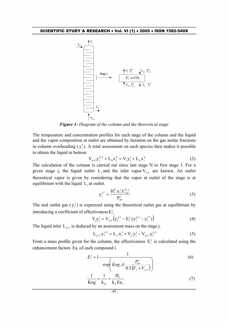
iy represent respectively the average composition in the gas phase leaving the stage j, the composition in the gas phase entering the stage j and the composition of the gas phase at equilibrium with the liquid phase leaving the stage j. This approach has the simple and fast advantage of being but the disadvantage of not considering with precision the transfer phenomena. The philosophy of this modeling is that the gas phase and the liquid phase are in equilibrium only at the gas-liquid interface and nowhere elsewhere. This representation is not completely satisfactory. The kinetics as well as the equilibrium constants of reactions depends on the local concentrations and the temperatures which can vary in an important way along the stage. Thus Higler et al. [8 - 10] developed a model of cells for the non equilibrium stage. The idea is to divide the stage into a certain number of contact cells. These cells represent a small zone of the stage where the liquid and gas compositions can be assumed homogeneous and by choosing in an adequate way the channeling and recirculation of fluids, the hydrodynamic problems and dead space can be apprehended. The columns with packing are very interesting in all the processes requiring large interfacial surface between two phases. The packing inside the columns can be arranged, thus offering a regular geometrical structure throughout the column, or not arranged as the Raschig rings which are distributed by chance within the column. In General, the arranged packing is preferred because the pressure loss is less and the column hydrodynamic parameters are accessible. MODELING OF REFERENCE’S ABSORPTION COLUMN The modeling of the reference absorption columns is based on the use of the Murphee mass effectiveness, j

iE and of the thermal effectiveness, ETHj (Figure 1).


- 45 -

L 0

Ln

V n +1

V 1

Lj-1

Lj

Vj

Vj+1

Stage j et ETHj

jiE

LjT

L1jT−

G1jT+

GjT

Figure 1: Diagram of the column and the theoretical stage

The temperature and concentration profiles for each stage of the column and the liquid and the vapor composition at outlet are obtained by iteration on the gas molar fractions in column overheading ( 1

iy ). A total assessment on each species then makes it possible to obtain the liquid in bottom n

in1i1

0i0

1ni1n xLyVxLyV +=++

+ (2) The calculation of the column is carried out since last stage N to first stage 1. For a given stage j, the liquid outlet jL and the inlet vapor 1jV + are known. An outlet theoretical vapor is given by considering that the vapor at outlet of the stage is at equilibrium with the liquid jL at outlet.

jtot

j,Ltot

ji

Si,*j

i PC.x.H

y = (3)

The real outlet gas ( jiy ) is expressed using the theoretical outlet gas at equilibrium by

introducing a coefficient of effectiveness jiE .

( ))yy.(Ey.VyV ,*ji

1ji

ji

1ji1j

jij −−= ++

+ (4) The liquid inlet 1jL − is deduced by an assessment mass on the stage j.

1ji1j

jij

jij

1ji1j y.Vy.Vx.Lx.L +

+−

− −+= (5)

From a mass profile given for the column, the effectiveness jiE is calculated using the

enhancement factors iEa of each compound i.

( )

+

−=

+1.5.0..exp

11

jj

jtot

ji

VVPAKog

E

(6)

iL

i

G EakH

k1

Kog1

+=

(7)


- 46 -

Kog , A and jtotP represent respectively the gas side mass transfer coefficient, the

interfacial area and total pressure at the stage j. Enhancement factors iEa for each compound i which transfers from the gas phase to the liquid phase are calculated thanks to the Hatta number (Ha).

)Hatanh(HaEa i =

(8)

In the case of CO2:

( )L

esminAamOHOHLCO

k

CkCkDHa 2

+=

−

(9)

the terms kOH and kam represent the constant kinetics of the reactions between CO2 and OH- and CO2 and the alkanolamine. The composition of the outgoing vapor of the first stage is compared with the initial composition at the overhead then this one is modified until obtaining convergence of the column on the following criterion:

ε≤−

init,1i1

calc,1i1

init,1i1

yVyVyV

(10) The calculation of the thermal profile of the absorption column uses a thermal effectiveness th

jE at the stage j. The calculation of the temperatures is carried out since the column’s bottom while going up towards the overhead. For a stage j, the temperature of the gas phase outgoing G

jT is calculated by:

( )G1j

Lj

thj

G1j

Gj TT.ETT ++ −+= (11)

thjE =1 is equivalent considering the liquid and outgoing gas in heat balance. By an

assessment enthalpic on the stage j, the enthalpy of the inlet liquid ( )L1j

L1j TH −− on the

stage j is given. ( ) ( ) ( ) ( )G

jGjj

Lj

Ljj

G1j

G1j1j

L1j

L1j1j TH.VTH.LTH.VTH.L +=+ +++−−− (12)

From the enthalpy of the liquid ( )L1j

L1j TH −− , the composition of the liquid 1jL − being

known, the temperature of the liquid L1jT − is deduced.

The convergence of the column temperature profiles is regarded as attack when the criterion translating the equality between the initial temperature at the column’s overhead and the temperature at the overhead recomputed is satisfied.

ε≤−

init,G1

calc,G1

init,G1

TTT

(13)

The modeling of the columns with the non equilibrium stage has the advantage of retranscribing reality. This modeling is very general-purpose since all the types of packing or stage columns and can be modeled easily. Many authors (Perez-Cisneros et al. [1], Scenna et al. [2], Sneesby et al. [3]) use the MESH equations in reactive separations cases. However reactive separations process is a having many similarities with the absorption and regeneration columns which we want to model. The reference simulation is based on the stage model, which describes the column as a


- 47 -

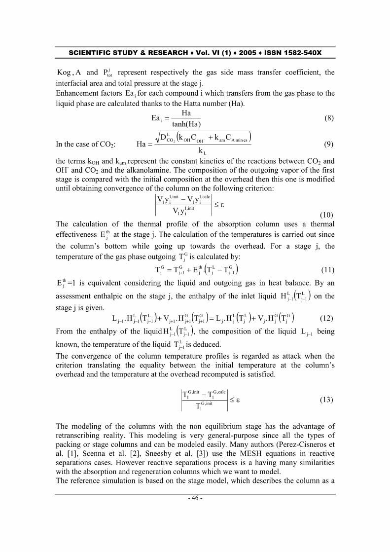
succession of stages at thermodynamic equilibrium. The transfer model is used to calculate an enhancement factor as well as a thermal effectiveness. This approach has the simple and effective advantage of being simpler. Our transfer model based on the double film theory makes it possible to know the flux transferred to the interface which can be expressed in the term of an enhancement factor and thus we can introduce our model within the industrial simulator easily. MODEL DESCRIPTION The first stage of this work is the development of a precise elementary model holding account of the mass transfer of multiconstituant as well as heat transfer in liquid film and the gas film (Figure 2). The theory used is that of the modified film of Chang and Rochelle [11] which gives results equivalent to the penetration theory while being simpler.

Figure 2: Schematic diagram of the two films model Mass transfer We make the assumption of an ideal and diluted liquid medium where water is the stagnant majority species. In this case, the Nernst-Planck equations are applied, in liquid film for [ ]LGG ;x δ+δδ∈ . NC components are considered. NR reactions take place of which NRI instantaneous reactions.

0)x(Rdx

))x(C*)x((dRTF

DZdx

)x(CdD iirdayL

ii2i

2Li =+

Φ∇− (14)

In this equation, the variation of the diffusion coefficient according to the position in liquid film is neglected. )x(R i represents the production term.

( )∑=

−−ν=RN

1kkkk,ii )x(r)x(r.)x(R (15)

k,iν , kr , kr− represent respectively the stoechiometric coefficient of compound i and the

Bulk gas Bulk liquid Gas film Liquid film

Gδ0 LG δ+δ

liquidbulkkC

liquidbulkiC

x

)x(Ck

)x(C i

gasbulkiP

intiP

intiC

iN


- 48 -

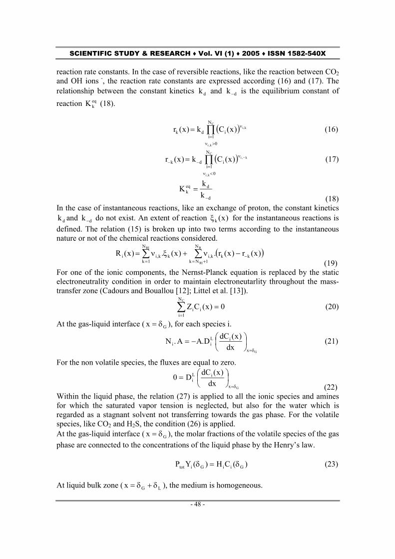
reaction rate constants. In the case of reversible reactions, like the reaction between CO2 and OH ions -, the reaction rate constants are expressed according (16) and (17). The relationship between the constant kinetics dk and dk − is the equilibrium constant of reaction eq

kK (18).

( )∏>ν=

ν=C

k,i

k,iN

01i

idk )x(Ck)x(r (16)

( )∏<ν=

ν−−

−=C

k,i

k,iN

01i

idk )x(Ck)x(r (17)

d

deqk k

kK

−

= (18)

In the case of instantaneous reactions, like an exchange of proton, the constant kinetics dk and dk − do not exist. An extent of reaction )x(kξ for the instantaneous reactions is

defined. The relation (15) is broken up into two terms according to the instantaneous nature or not of the chemical reactions considered.

( )∑∑

+=−

=−ν+ξν=

R

RI

RI N

1Nkkkk,i

N

1kkk,ii )x(r)x(r.)x(.)x(R

(19) For one of the ionic components, the Nernst-Planck equation is replaced by the static electroneutrality condition in order to maintain electroneutarlity throughout the mass-transfer zone (Cadours and Bouallou [12]; Littel et al. [13]).

∑=

=CN

1iii 0)x(CZ (20)

At the gas-liquid interface ( Gx δ= ), for each species i.

Gx

iLii dx

)x(dCD.AA.Nδ=

−= (21)

For the non volatile species, the fluxes are equal to zero.

Gx

iLi dx

)x(dCD0δ=

=

(22) Within the liquid phase, the relation (27) is applied to all the ionic species and amines for which the saturated vapor tension is neglected, but also for the water which is regarded as a stagnant solvent not transferring towards the gas phase. For the volatile species, like CO2 and H2S, the condition (26) is applied. At the gas-liquid interface ( Gx δ= ), the molar fractions of the volatile species of the gas phase are connected to the concentrations of the liquid phase by the Henry’s law. )(CH)(YP GiiGitot δ=δ (23) At liquid bulk zone ( LGx δ+δ= ), the medium is homogeneous.


- 49 -

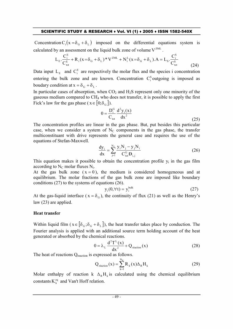
Concentration ( )LGi xC δ+δ= imposed on the differential equations system is calculated by an assessment on the liquid bulk zone of volume ZMLV .

Stot

Si

SLGLi

ZMLLGiE

tot

Ei

E CC

.LA).x(NV*)x(RCC

.L =δ+δ=+δ+δ=+ (24)

Data input EL and EiC are respectively the molar flux and the species i concentration

entering the bulk zone and are known. Concentration SiC outgoing is imposed as

boudary condition at LGx δ+δ= . In particular cases of absorption, when CO2 and H2S represent only one minority of the gaseous medium compared to CH4 who does not transfer, it is possible to apply the first Fick’s law for the gas phase ( [ ]G;0x δ∈ ).

2

i2

tot

Gi

dx)x(yd

CD0 =

(25) The concentration profiles are linear in the gas phase. But, put besides this particular case, when we consider a system of NC components in the gas phase, the transfer multiconstituant with drive represents the general case and requires the use of the equations of Stefan-Maxwell.

∑=

−=

CN

1j j,iGtot

ijjii

DCNyNy

dxdy (26)

This equation makes it possible to obtain the concentration profile yi in the gas film according to NC molar fluxes Ni. At the gas bulk zone ( 0x = ), the medium is considered homogeneous and at equilibrium. The molar fractions of the gas bulk zone are imposed like boundary conditions (27) to the systems of equations (26). bulk

ii y)t,0(y =∀ (27) At the gas-liquid interface ( Gx δ= ), the continuity of flux (21) as well as the Henry’s law (23) are applied. Heat transfer Within liquid film ( [ ]LGG ;x δ+δδ∈ ), the heat transfer takes place by conduction. The Fourier analysis is applied with an additional source term holding account of the heat generated or absorbed by the chemical reactions.

)x(Qdx

)x(Td0 réaction2

L2

L +λ= (28)

The heat of reactions Qreaction is expressed as follows.

∑=

∆=RN

1kkRkréaction H)x(R)x(Q (29)

Molar enthalpy of reaction k kR H∆ is calculated using the chemical equilibrium constants eq

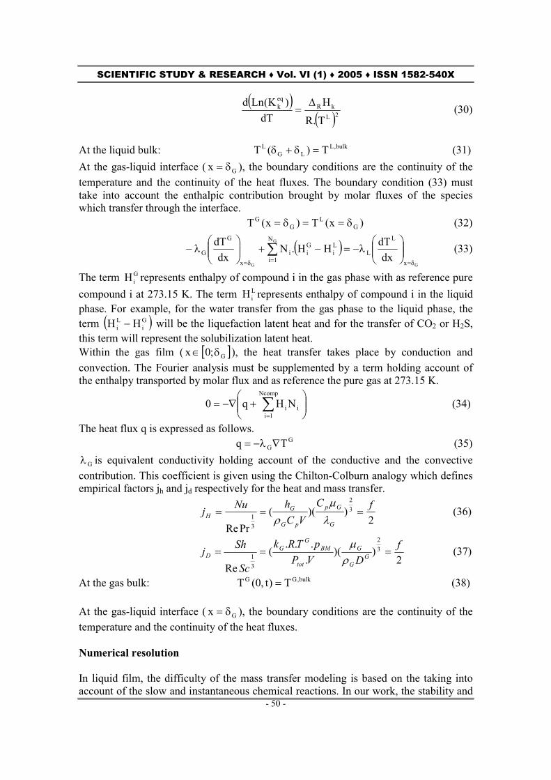
kK and Van't Hoff relation.


- 50 -

( )

( )2LkR

eqk

T.R

HdT

)K(Lnd ∆= (30)

At the liquid bulk: bulk,L

LGL T)(T =δ+δ (31)

At the gas-liquid interface ( Gx δ= ), the boundary conditions are the continuity of the temperature and the continuity of the heat fluxes. The boundary condition (33) must take into account the enthalpic contribution brought by molar fluxes of the species which transfer through the interface. )x(T)x(T G

LG

G δ==δ= (32)

( )G

G

G x

L

L

N

1i

Li

Gii

x

G

G dxdTHH.N

dxdT

δ==δ=

λ−=−+

λ− ∑ (33)

The term GiH represents enthalpy of compound i in the gas phase with as reference pure

compound i at 273.15 K. The term LiH represents enthalpy of compound i in the liquid

phase. For example, for the water transfer from the gas phase to the liquid phase, the term ( )G

iLi HH − will be the liquefaction latent heat and for the transfer of CO2 or H2S,

this term will represent the solubilization latent heat. Within the gas film ( [ ]G;0x δ∈ ), the heat transfer takes place by conduction and convection. The Fourier analysis must be supplemented by a term holding account of the enthalpy transported by molar flux and as reference the pure gas at 273.15 K.

+−∇= ∑

=

Ncomp

1iii NHq0 (34)

The heat flux q is expressed as follows. G

G Tq ∇λ−= (35)

Gλ is equivalent conductivity holding account of the conductive and the convective contribution. This coefficient is given using the Chilton-Colburn analogy which defines empirical factors jh and jd respectively for the heat and mass transfer.

2))((

PrRe

32

31

fCVC

hNujG

Gp

pG

GH ===

λµ

ρ (36)

2))(

....

(Re

32

31

fDVP

pTRk

Sc

Shj GG

G

tot

BMG

GD ===

ρµ

(37)

At the gas bulk: bulk,GG T)t,0(T = (38) At the gas-liquid interface ( Gx δ= ), the boundary conditions are the continuity of the temperature and the continuity of the heat fluxes. Numerical resolution In liquid film, the difficulty of the mass transfer modeling is based on the taking into account of the slow and instantaneous chemical reactions. In our work, the stability and


- 51 -

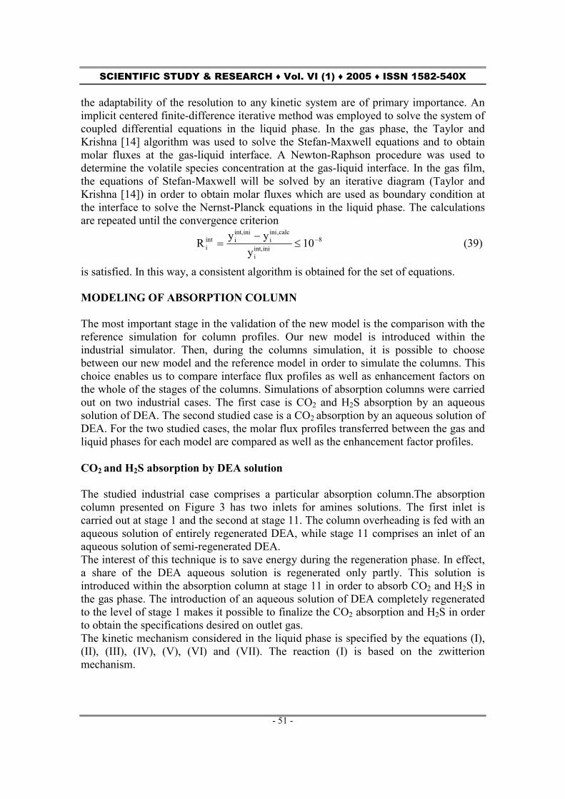
the adaptability of the resolution to any kinetic system are of primary importance. An implicit centered finite-difference iterative method was employed to solve the system of coupled differential equations in the liquid phase. In the gas phase, the Taylor and Krishna [14] algorithm was used to solve the Stefan-Maxwell equations and to obtain molar fluxes at the gas-liquid interface. A Newton-Raphson procedure was used to determine the volatile species concentration at the gas-liquid interface. In the gas film, the equations of Stefan-Maxwell will be solved by an iterative diagram (Taylor and Krishna [14]) in order to obtain molar fluxes which are used as boundary condition at the interface to solve the Nernst-Planck equations in the liquid phase. The calculations are repeated until the convergence criterion

8iniint,

i

calc,inii

iniint,iint

i 10y

yyR −≤

−=

(39)

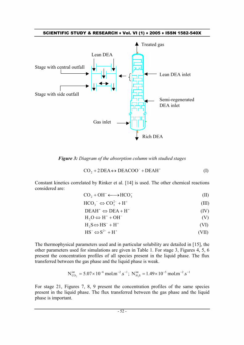
is satisfied. In this way, a consistent algorithm is obtained for the set of equations. MODELING OF ABSORPTION COLUMN The most important stage in the validation of the new model is the comparison with the reference simulation for column profiles. Our new model is introduced within the industrial simulator. Then, during the columns simulation, it is possible to choose between our new model and the reference model in order to simulate the columns. This choice enables us to compare interface flux profiles as well as enhancement factors on the whole of the stages of the columns. Simulations of absorption columns were carried out on two industrial cases. The first case is CO2 and H2S absorption by an aqueous solution of DEA. The second studied case is a CO2 absorption by an aqueous solution of DEA. For the two studied cases, the molar flux profiles transferred between the gas and liquid phases for each model are compared as well as the enhancement factor profiles. CO2 and H2S absorption by DEA solution The studied industrial case comprises a particular absorption column.The absorption column presented on Figure 3 has two inlets for amines solutions. The first inlet is carried out at stage 1 and the second at stage 11. The column overheading is fed with an aqueous solution of entirely regenerated DEA, while stage 11 comprises an inlet of an aqueous solution of semi-regenerated DEA. The interest of this technique is to save energy during the regeneration phase. In effect, a share of the DEA aqueous solution is regenerated only partly. This solution is introduced within the absorption column at stage 11 in order to absorb CO2 and H2S in the gas phase. The introduction of an aqueous solution of DEA completely regenerated to the level of stage 1 makes it possible to finalize the CO2 absorption and H2S in order to obtain the specifications desired on outlet gas. The kinetic mechanism considered in the liquid phase is specified by the equations (I), (II), (III), (IV), (V), (VI) and (VII). The reaction (I) is based on the zwitterion mechanism.


- 52 -

Figure 3: Diagram of the absorption column with studied stages

+− +↔+ DEAHDEACOODEA2CO2 (I) Constant kinetics correlated by Rinker et al. [14] is used. The other chemical reactions considered are: −− →←+ 32 HCOOHCO (II)

+−− +⇔ HCOHCO 233 (III)

++ +⇔ HDEADEAH (IV) −+ +⇔ OHHOH2 (V) +− +⇔ HHSSH2 (VI) +−− +⇔ HSHS 2 (VII) The thermophysical parameters used and in particular solubility are detailed in [15], the other parameters used for simulations are given in Table 1. For stage 3, Figures 4, 5, 6 present the concentration profiles of all species present in the liquid phase. The flux transferred between the gas phase and the liquid phase is weak. 126int

CO s.m.mol1007.5N2

−−−×= ; 125intSH s.m.mol1049.1N

2

−−−×= For stage 21, Figures 7, 8, 9 present the concentration profiles of the same species present in the liquid phase. The flux transferred between the gas phase and the liquid phase is important.

Treated gas

Lean DEA inlet

Semi-regenerated DEA inlet

Gas inlet

Rich DEA

Stage with central outfall

Stage with side outfall

Lean DEA


- 53 -

123intCO s.m.mol1053.3N

2

−−−×= ; 122intSH s.m.mol1030.1N

2

−−−×= Comparison of these profiles is interesting because stage 3, located in top of the column, is fed by an aqueous solution of DEA slightly acid gas loaded and the gas phase then contains a weak molar fraction of CO2 and H2S, while stage 21 is fed by an aqueous solution of DEA strongly acid gas loaded; then the gas phase contains a proportion much more important of CO2 and of H2S.

Table 1: Parameters used Gas to be treated Lean amine Semi-regenerated amine Pression (105 Pa) 67.5 66.9 61.0 Temperature (K) 325.15 324.64 324.50 Composition

72.0y18.0y042.0y

4

2

2

CH

SH

CO

===

102.0x896.0x106x

109.2x

DEA

OH

4SH

4CO

2

2

2

==

×=×=

−

−

081.0x9103.0x

1067x102x

DEA

OH

4SH

3CO

2

2

2

==

×=×=

−

−

Flux rate (mol.s-1) 3778 6501 8228 The comparison between Figure 4 and Figure 8 shows a H2S profile in the liquid phase completely different. For stage 3, the liquid is slightly loaded, the concentration in hydronium ions is important at the interface; it is much higher than the H2S concentration.

33intSH m.mol1083.3C

2

−−×= ;

3intOH m.mol42.1C −=−

The H2S absorption is then entirely under kinetic control, which explains the shape of the very similar curve to that of CO2 absorption. For stage 21, the aqueous DEA solution is strongly acid gases loaded and H2S flux at the interface is important. The concentration in hydronium ions at the interface is of the same order of magnitude as the H2S concentration.

31intSH m.mol1063.2C

2

−−×= ;

31intOH m.mol1016.2C −−×=−

The H2S absorption depends then only on the OH- ions diffusion within liquid film, which explains the linear profile of the H2S concentration within liquid film. For stage 3, CO2 absorbed is transformed by the chemical reactions into carbonates and hydrogen carbonates ions in weak concentrations. On the other hand, for the stage 21, CO2 is transformed mainly into carbamates ions, while the concentrations in carbonates and hydrogen carbonates ions are close. On Figures 10, 11, 12, CO2 and H2S molar fluxes as well as the CO2 and H2S enhancement factors are compared for the reference model within the simulator and our model. The visible change of slope in all the curves between stage 10 and stage 11 corresponds to the introduction within the column of aqueous semi-regenerated DEA solution. Figure 10 presents the comparison of molar CO2 and H2S fluxes between our new model and the reference model. A general shape of the molar flux curves according to N° of stage is identical between the two models. Nevertheless, differences between CO2 fluxes are on average respectively 15 % for the first 10 stages and 22 % for the following stages. For H2S, the average deviation between the curves is 20 %. Figure 13 presents the comparison of molar flux between our new model and the reference model.


- 54 -

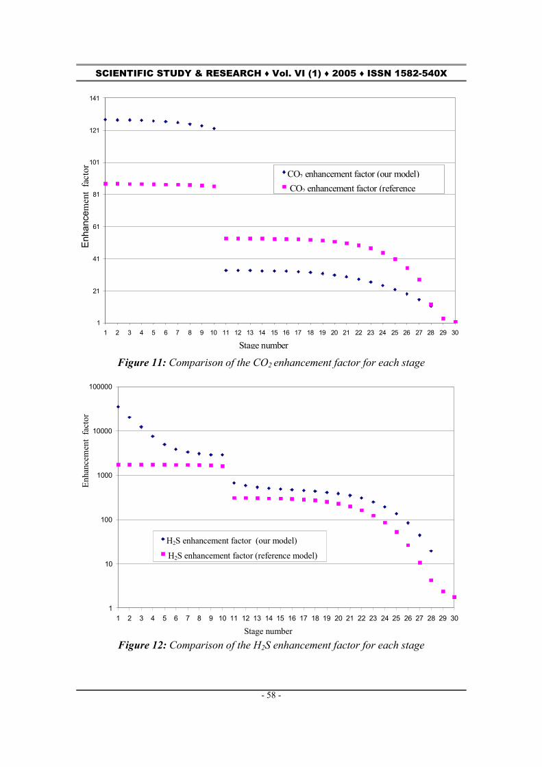
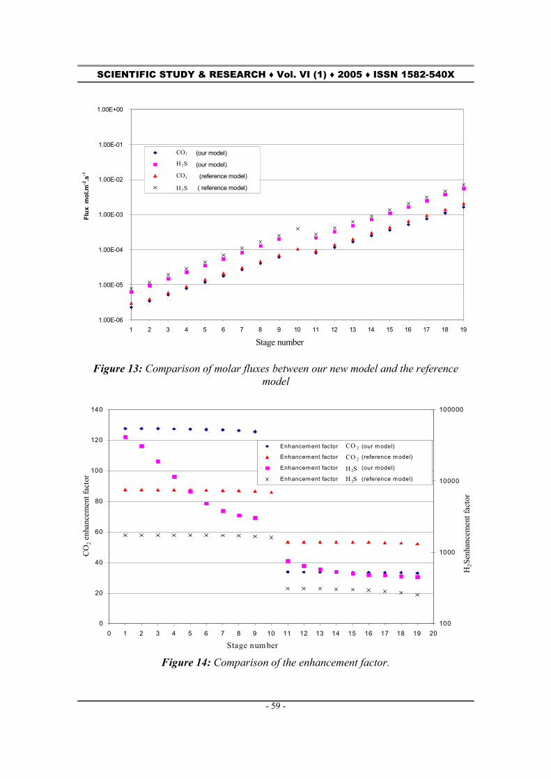
The average deviation between the CO2 flux calculated with our new model and the CO2 flux calculated with the reference model is 12 %. For H2S the variation is 20% on average. For H2S, this variation remains the same one. Figure 14 presents the CO2 and H2S fluxes at the gas-liquid interface. The comparison of the CO2 and H2S enhancement factors between our new model and the reference model is presented in Figures 11 and 12. The first observation is the important difference between the enhancement factors calculated with our new model and those calculated with the reference model. For CO2 (Figure 11 and Figure 14), for the first 10 stages, the average deviation is 30 % and this variation goes up to 35 % between stages 11 to 27. For H2S (Figure 12 and Figure 14), the average deviation between the enhancement factor curves of each model is 42 %. The enhancement factor is calculated using interfacial flux but also using the gradient of concentration between the interface and the liquid bulk. However this gradient of concentration is different between the two models what explains why the differences between the enhancement factors of the two models are higher than the difference between fluxes at the interface. The tendencies of enhancement factor curves can nevertheless be compared between the two models. With regard to the CO2 enhancement factor, the profiles of the curves are similar between our new model and the reference model. On the other hand, for H2S, the profile of the enhancement factor curve for our new model is different from that of the reference model. Indeed, the enhancement factor with our new model increases much for the first column stages where the liquid phase is slightly loaded, which is more realistic than the almost stage profile of the enhancement factor curve with the reference model for the first 10 stages. The average deviation of 20 % noted between the new model and the reference model has several causes. We already noted that with the same transfer model, an average deviation of 10 % appears when a different kinetic model for the reaction between CO2 and the DEA is considered. On the other hand, it appears clearly that the successive iterations on the simulation of the column modify the fluxes values only of 2 % at most. The remainder of the difference is then directly ascribable with the transfer model.

Figure 4: CO2 and H2S concentration profiles in liquid film for stage 3

0.04

0.05

0.06

0.07

0.08

0.09

0.10

0.11

0.12

0.13

0.14

0 0.1 0.2 0.3 0.4 0.5 0.6 0.7 0.8 0.9 1 Dimensionless liquid film

CO

2 con

cent

ratio

n 10

-3 m

ol.m

-3

3.825

3.826

3.826

3.827

3.827

3.828

3.828

3.829

3.829

3.830

3.830

H2S

con

cent

ratio

n 10

-3 m

ol.m

-3

CO2 concentration

H2S concentration


- 55 -

Figure 5: H+ and OH-concentration profiles in liquid film for stage 3

Figure 6: concentration profiles in liquid film (stage 3)

37.800

37.804

37.808

37.812

37.816

0 0.1 0.2 0.3 0.4 0.5 0.6 0.7 0.8 0.9 1Dimensionless liquid film

3884.52

3884.53

3884.54

DEA

mol

.m-3

DEAH+ concentrationDEA concentration

+

8.4524

8.4526

8.4528

8.4530


-

- DEACOO- concentration

0.7080

0.7084

0.7088

0.7092


2.0160

2.0166

2.0172

2.0178

HCO3- concentration

CO32- concentration3

23.015

23.020

23.025

23.030


-

HS- m

ol.m

-3

8.4015

8.4016

8.4017

8.4018

8.4019

S- 10

-2 m

ol.m

-3

HS- concentration S2- concentration

CO

3-- m

ol.m

-3

HC

O3- m

ol.m

-3

DEA

CO

O-

mol

.m-3

D

EAH

+m

ol.m

-3

1.4205

1.4206

1.4207

1.4208

1.4209

1.4210

0 0.1 0.2 0.3 0.4 0.5 0.6 0.7 0.8 0.9 1

Dimensionless liquid film

OH

- con

cent

ratio

n m

ol.m

-3

5.2460

5.2464

5.2468

5.2472

5.2476

5.2480

5.2484

H+ c

once

ntra

tion

mol

.m-3

OH- concentration

H+ concentration


- 56 -

Figure 7: concentration profiles in liquid film (stage 21)

0

20

40

60

80

100

120

140

160

180

200

0 0.1 0.2 0.3 0.4 0.5 0.6 0.7 0.8 0.9 1 Dimensionless liquid film

CO

2 con

cent

ratio

n 10

-3 m

ol.m

-

3

200

210

220

230

240

250

260

270

H2S

con

cent

ratio

n 10

-3 m

ol.m

-3

CO2 concentration

H2S concentration

Figure 8: CO2 and H2S concentration profiles in liquid film (stage 21)

3230

3250

3270

3290

0 0.1 0.2 0.3 0.4 0.5 0.6 0.7 0.8 0.9 1


DEA

mol

.m-3

260

280

300

DEA concentration DEAH+ concentration

51

52

53

54


-

DEACOO- concentration

3

6

9


-

HCO3- concentration

CO32- concentration

195

205

215

225


HS- m

ol.m

-3

0.164

0.165

0.166

0.167

0.168

S-- m

ol.m

-3

HS- concentration S2- concentration

DEA

CO

O- m

ol.m

-3

HC

O3- ,

CO

32- m

ol.m

-3

DEA

H+ m

ol.m

-3


- 57 -

Figure 9: OH- and H+ concentration profiles in the liquid film (stage 21)

Figure 10: Comparison of molar fluxes (gas and liquid phases) for each stage

0.20

0.22

0.24

0.26

0 0.1 0.2 0.3 0.4 0.5 0.6 0.7 0.8 0.9 1


OH

- con

cent

ratio

n m

ol.m

-3

4.7

4.9

5.1

5.3

5.5

H+ c

once

ntra

tion

10-7

mol

.m-3

+

OH- concentrationH+ concentration

1.00E-06

1.00E-05

1.00E-04

1.00E-03

1.00E-02

1.00E-01

1.00E+00

1 2 3 4 5 6 7 8 9 10 11 12 13 14 15 16 17 18 19 20 21 22 23 24 25 26 27 28 29 30

Stage number

Flux

mol

.m-2

.s-1

CO2 (our model)

CO2 (reference model)

H2S (our model) H2S (reference model)


- 58 -

Figure 11: Comparison of the CO2 enhancement factor for each stage

1

10

100

1000

10000

100000

1 2 3 4 5 6 7 8 9 10 11 12 13 14 15 16 17 18 19 20 21 22 23 24 25 26 27 28 29 30

Stage number

E

nhan

cem

ent

fact

or

H2S enhancement factor (our model)

H2S enhancement factor (reference model)

Figure 12: Comparison of the H2S enhancement factor for each stage

1

21

41

61

81

101

121

141

1 2 3 4 5 6 7 8 9 10 11 12 13 14 15 16 17 18 19 20 21 22 23 24 25 26 27 28 29 30

Stage number

Enha

ncem

ent

fact

or

CO2 enhancement factor (our model) CO2 enhancement factor (reference


- 59 -

1.00E-06

1.00E-05

1.00E-04

1.00E-03

1.00E-02

1.00E-01

1.00E+00

1 2 3 4 5 6 7 8 9 10 11 12 13 14 15 16 17 18 19

Stage number

Flux

mol

.m-2

.s-1

(our model) (our model) (reference model)

( reference model)

2 CO S H 2 2 CO S H 2

Figure 13: Comparison of molar fluxes between our new model and the reference model

Figure 14: Comparison of the enhancement factor.

0

20

40

60

80

100

120

140

0 1 2 3 4 5 6 7 8 9 10 11 12 13 14 15 16 17 18 19 20

Stage number

CO

2 enh

ance

men

t fac

tor

100

1000

10000

100000

H2S

enha

ncem

ent f

acto

r

Enhancement factor (our model)

Enhancement factor (reference model)

Enhancement factor (our model)

Enhancement factor (reference model)

2CO

SH 2

2CO

SH 2


- 60 -

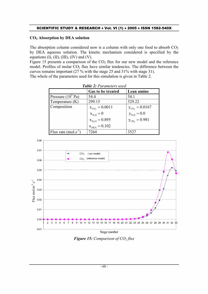
CO2 Absorption by DEA solution The absorption column considered now is a column with only one food to absorb CO2 by DEA aqueous solution. The kinetic mechanism considered is specified by the equations (I), (II), (III), (IV) and (V). Figure 15 presents a comparison of the CO2 flux for our new model and the reference model. Profiles of molar CO2 flux have similar tendencies. The difference between the curves remains important (27 % with the stage 25 and 31% with stage 31). The whole of the parameters used for this simulation is given in Table 2.

Table 2: Parameters used Gas to be treated Lean amine Pressure (105 Pa) 54.4 54.1 Temperature (K) 299.15 329.22 Composition

102.0x895.0x

0x0011.0x

DEA

OH

SH

CO

2

2

2

====

981.0y0.0y0167.0y

4

2

2

CH

SH

CO

===

Flux rate (mol.s-1) 7264 3527

Figure 15: Comparison of CO2 flux

-0.01

0.00

0.01

0.02

0.03

0.04

0.05

0.06

0.07

0.08

1 2 3 4 5 6 7 8 9 10 11 12 13 14 15 16 17 18 19 20 21 22 23 24 25 26 27 28 29 30 31 32 33

Stage number

Flux

mol

.m-2

.s-1

( our model)

(reference model)

2CO

2CO


- 61 -

CONCLUSION This study shows that the profiles obtained by our model are in accordance with the awaited results. At the column’s overhead, the liquid is slightly acid gas loaded and CO2 and H2S absorption is entirely under kinetic control. In column’s bottom, the liquid is strongly acid gases loaded, the H2S absorption is then under diffusional control. The comparison of the CO2 and H2S enhancement factor profiles given by the two models show very consequent variations (respectively 30 and 40 %), whereas the difference between absorption rate is only 20 % on average. This important variation can be allotted to the difference between the gradients of concentration of the liquid phase for the two models. A variation of 12 % for the CO2 absorption rate and of 20 % for the H2S absorption rate between our model and the reference model confirms the good agreement between the two models. Our computer code also represents CO2 absorption in an aqueous solution of DEA with an average deviation of 20 % with respect to the reference model. This variation is explained by the difference between the models in the taking into account of heat and mass transfer phenomena. Experiments on a pilot column are in hand. These measurements of the CO2 and H2S absorption by the DEA will make it possible to compare the results provided by our model but also those provided by the reference model with the experimental results and thus to determine which models is able to represent the absorption columns well. The industrial interest of our model is the taking into account in a more realistic and more complete way of the heat and mass transfer phenomena compared to the reference model. Its principal advantages are to be able to model any whole of chemical reactions. The taking account of new chemical compounds, like the mercaptans or new reactions is easy. NOMENCLATURE A ...................Interfacial area (m2 / m3)

iC ..................Molar concentration, mol.m-3 vC ..................Heat capacity of component i, J.mol-1.K-1

id ...................Driving force, m-1 SiD or iD ......Diffusivity, m2.s-1

j,iD ................Stefan-Maxwell diffusivity, m2.s-1 iEa ................Enhancement factor

jiE ..................Mass effectiveness thjE .................Thermal effectiveness

F ....................Faraday’s constant 96500 C/mol Ha .................Hatta number

SiH or iH ......Henry’s law constant in the concentration scale, Pa.m3.mol-1

GjH .................Molar enthalpy, J.mol-1


- 62 -

iJ ...................Molar diffusion flux of species i, mol.m-2.s-1

eqkK ................Equilibrium constant of reaction k

Gk .................Gas side mass transfer coefficient, mol-1.m-2.Pa-1.s-1 Lk ..................Liquid side mass transfer coefficient, m.s-1

k .....................Rate coefficient L.....................Liquid molar flux, mol.s-1

iM .................Molar mass, g.mol-1 CN .................Number of diffusing species GN .................Number of volatiles species RN .................Total number of reactions totN ................Molar flux, mol.m-2.s-1

Nu ..................Nusselt number P ...................Pressure, Pa q .....................Energy flux, en W.m-2

réactionQ ..........Heat of reactions, W.m-3 Re .................Reynolds number

iR ..................Rate of production of i due to chemical reaction en mol.s-1 ijR ..................Residual (Newton-Raphson method)

Sc ...................Schmidt number Sh...................Sherwood number t ....................Time, s T ...................Temperature, K

iu ...................Velocity, m.s-1 VS...................Molar volume, m3.mol-1

iV ...................Vapor fluxrate, mol.s-1 x ....................Coordinate, m

jix ...................Liquid mole fraction, mol/mol jiy ...................Gas mole fraction, mol/mol iZ ...................Ionic charge of component i

Greek Letters:

iR H∆ .............Molar Enthalpy of reaction i, J.mol-1 ∆.....................Difference δ .....................Film thickness, m

j,iδ .................Kronecker delta ( j,iδ =1 for i = j, j,iδ =0 for i#j)


- 63 -

Φ ...................Electrostatic potential, V.m-1 ∑

∑ ∂

∂

qq

Lq

q

qLq

xCDZ

xxC

DZ

FRT

q

q

)(

)(

2

Λ ....................Thermal conductivity, W.m-1.K-1 µ ....................Viscosity, 10-3 Pa.s (cP)

k,iν .................Stoichiometric coefficient ρ .....................Density, g.cm-3

Subscripts: Am .................Amine calc………….calculed ini………….. initial j……………..Stage j parameter tot ...................Total Superscripts: int, .................Interface parameter bulk ................Bulk phase L.....................liquid G ....................gas * .....................Equilibrium value Acknowledgements The authors wish to thank TOTAL for their financial support to this investigation. REFERENCES 1. Perez-Cisneros, E.; Schenk, M.; Gani, R.; Pilavachi, P.A.; Aspects of simulation,

design and analysis of reactive distillation operations. Comp. Chem. Eng. 1996, 20, S267.

2. Scenna, N. J.; Ruiz, C.A.; Benz, S.J.; Dynamic simulation of startup procedures of reactive distillation columns. Comp. Chem. Eng. 1998, 22, S719.

3. Sneesby M. G.; Tadé, M. O.; Smith, T. N. Steady-state transitions in the reactive distillation of MTBE. Comp. Chem. Eng. 1998, 22, 879.

4. Taylor, R.; Krishna, R.; Modelling reactive distillation. Chem. Eng. Sci. 2000, 55, 5183.

5. Baur, R.; Taylor, R.; Krishna, R.; Dynamic behaviour of reactive distillation columns described by a non equilibrium stage model. Chem. Eng. Sci. 2001, 56, 2085.


- 64 -

6. Isla, M. A.; Irazoqui, H. A.; Modeling, analysis, and simulation of a methyl tert-butyl ether reactive distillation column. Ind. Eng. Chem. Res. 1996, 35, 2396.

7. Lee, J. H.; Dudukovic, M. P.; A comparison of the equilibrium and non equilibrium models for a multicomponent reactive distillation column. Comp. Chem. Eng. 1998, 23, 159.

8. Higler, A. P.; Krishna R.; Taylor R.; A non equilibrium cell for multicomponent reactive separation processes. Am. Inst. Chem. Eng. J. 1999, 45, 2357.

9. Higler, A. P., Krishna, R.; Taylor, R.; A non equilibrium cell model for packed distillation columns. The influence of distribution. Ind. Eng. Chem. Res. 1999, 38, 3988.

10. Higler, A. P.; Krishna, R.; Taylor R.; The influence of mass transfer and liquid mixing on the performance or reactive distillation tray column. Chem. Eng. Sci. 1999, 54, 2873.

11. Chang, S.; Rochelle, G. T.; Mass transfer enhanced by equilibrium reaction. Ind. Eng. Chem. Fund. 1982, 21, 379.

12. Cadours, R.; Bouallou, C.; Rigorous simulation of gas absorption into aqueous solutions. Ind. Eng. Chem. Res. 1998, 37, 1063.

13. Little, R. J.; Filmer, B.; Versteeg, G. F.; van Swaaij, W. P. M.; Modelling of simultaneous absorption of H2S and CO2 in alkanolamine solutions: the influence of parallel and consecutive reversible reactions and the coupled diffusion of ionic species. Chem. Eng. Sc. 1991, 46, 9, 2303.

14. Rinker, E. B.; Ashour, S. S.; Sandall, O. C.; Kinetics and modeling of carbon dioxide absorption into aqueous solutions of diethanolamine. Ind. Eng. Chem. Res. 1996, 35, 1107.

15. Vinel, D-J.; Bouallou, C.; Propriètés physico-chimiques des solutions aqueuses d’alcanolamines utilisées dans le traitement du gaz. Scientific Study & Research 2004, V(1-2), 11.

Documents

MODELING OF ACID GASES ABSORPTION COLUMN USING