Embed Size (px)
Citation preview
Linköpings universitet | Institutionen för
datavetenskap
Kandidatarbete | Utbildning - programområde
Vårterminen 2016 | LIU-IDA/LITH-EX-G-16/070--SE
Simulering av skalbara
strömningsprotokoll vid
användning av trådlös
flersändning/bredsändning
Simulation of Scalable Streaming Protocols using Wireless
Multicast/Broadcast
Christoffer Johansson
Martin Sjödin Jonsson
Handledare: Niklas Carlsson
Examinator: Nahid Shahmehri
Linköpings universitet
SE-581 83 Linköping
013-28 10 00, www.liu.se
Linköpings universitet
SE-581 83 Linköping

Abstract
In a society where the popularity of mobile video streaming increases, the need to un-
derstand the affect on the power consumption on mobile devices increases. This thesis
looks into which broadcasting protocol to use when trying to optimize the energy con-
sumption and startup delay while receiving a video from a transmitting source using scal-
able streaming protocols. This thesis evaluates four different scalable streaming protocols
and how much power mobile clients consume when receiving a video over different num-
ber of channels and how different interfaces such as 3G and WiFi affect the power con-
sumption. The protocols are simulated using our own written simulator and a tool called
EnergyBox, which simulates both 3G and WiFi connections. The thesis also compares the
protocols with each other in two ways, the amount of energy consumed and how long
the startup delay is for each protocol. Based on these simulations and comparisons we
conclude which protocol of these four provides the best energy-delay tradeoff. The result
shows that the energy consumption while using WiFi is much less than when using 3G. Fast
Broadcasting is also far superior the other protocols when it comes to energy consumption.
When it comes to startup delay the protocols are very even.

Acknowledgments
First and foremost we would like to express our gratitude to our supervisor Niklas Carlsson,for answering all of our questions and providing us with useful advice when conducting thisstudy. Furthermore, we would like to thank Ekhiotz Jon Vergara for answering our questionsregarding EnergyBox.
iv

Contents
Abstract iii
Acknowledgments iv
Contents v
List of Figures vii
List of Tables ix
1 Introduction 1
1.1 Motivation . . . . . . . . . . . . . . . . . . . . . . . . . . . . . . . . . . . . . . . . 11.2 Aim . . . . . . . . . . . . . . . . . . . . . . . . . . . . . . . . . . . . . . . . . . . . 11.3 Research Questions . . . . . . . . . . . . . . . . . . . . . . . . . . . . . . . . . . . 11.4 Limitations . . . . . . . . . . . . . . . . . . . . . . . . . . . . . . . . . . . . . . . . 2
2 Background 3
2.1 Broadcast . . . . . . . . . . . . . . . . . . . . . . . . . . . . . . . . . . . . . . . . . 32.2 Multicast . . . . . . . . . . . . . . . . . . . . . . . . . . . . . . . . . . . . . . . . . 32.3 Periodic Broadcast Protocol . . . . . . . . . . . . . . . . . . . . . . . . . . . . . . 42.4 Pyramid Broadcasting . . . . . . . . . . . . . . . . . . . . . . . . . . . . . . . . . 42.5 Permutation-based Pyramid Broadcasting . . . . . . . . . . . . . . . . . . . . . . 42.6 Optimized Periodic Broadcasting Protocol . . . . . . . . . . . . . . . . . . . . . . 52.7 Fast Broadcasting Protocol . . . . . . . . . . . . . . . . . . . . . . . . . . . . . . . 52.8 Skyscraper Broadcasting . . . . . . . . . . . . . . . . . . . . . . . . . . . . . . . . 62.9 Harmonic Broadcasting . . . . . . . . . . . . . . . . . . . . . . . . . . . . . . . . 72.10 Energy Model . . . . . . . . . . . . . . . . . . . . . . . . . . . . . . . . . . . . . . 7
3 Method 10
3.1 EnergyBox . . . . . . . . . . . . . . . . . . . . . . . . . . . . . . . . . . . . . . . . 103.2 Simulator . . . . . . . . . . . . . . . . . . . . . . . . . . . . . . . . . . . . . . . . . 113.3 Wireshark . . . . . . . . . . . . . . . . . . . . . . . . . . . . . . . . . . . . . . . . 123.4 Experiment and Design . . . . . . . . . . . . . . . . . . . . . . . . . . . . . . . . 12
4 Results 14
4.1 Pyramid Broadcasting . . . . . . . . . . . . . . . . . . . . . . . . . . . . . . . . . 144.2 Optimized Periodic Broadcasting . . . . . . . . . . . . . . . . . . . . . . . . . . . 164.3 Fast Broadcasting . . . . . . . . . . . . . . . . . . . . . . . . . . . . . . . . . . . . 194.4 Skyscraper Broadcasting . . . . . . . . . . . . . . . . . . . . . . . . . . . . . . . . 214.5 Protocol Comparison . . . . . . . . . . . . . . . . . . . . . . . . . . . . . . . . . . 24
5 Discussion 30
5.1 Limitations . . . . . . . . . . . . . . . . . . . . . . . . . . . . . . . . . . . . . . . . 30
v
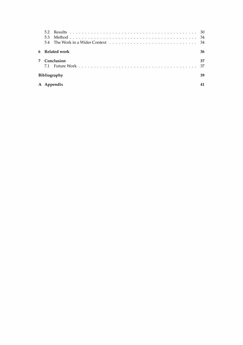
5.2 Results . . . . . . . . . . . . . . . . . . . . . . . . . . . . . . . . . . . . . . . . . . 305.3 Method . . . . . . . . . . . . . . . . . . . . . . . . . . . . . . . . . . . . . . . . . . 345.4 The Work in a Wider Context . . . . . . . . . . . . . . . . . . . . . . . . . . . . . 34
6 Related work 36
7 Conclusion 37
7.1 Future Work . . . . . . . . . . . . . . . . . . . . . . . . . . . . . . . . . . . . . . . 37
Bibliography 39
A Appendix 41
List of Figures
2.1 Pyramid Broadcasting Protocol . . . . . . . . . . . . . . . . . . . . . . . . . . . . . . 42.2 Optimized Periodic Broadcasting Protocol . . . . . . . . . . . . . . . . . . . . . . . . 52.3 Fast Broadcasting Protocol . . . . . . . . . . . . . . . . . . . . . . . . . . . . . . . . . 62.4 Skyscraper Broadcasting . . . . . . . . . . . . . . . . . . . . . . . . . . . . . . . . . . 72.5 EnergyBox State Machine for 3G (a) and WiFi (b) . . . . . . . . . . . . . . . . . . . . 82.6 RRC State Machine . . . . . . . . . . . . . . . . . . . . . . . . . . . . . . . . . . . . . 9
3.1 EnergyBox . . . . . . . . . . . . . . . . . . . . . . . . . . . . . . . . . . . . . . . . . . 113.2 Even mode . . . . . . . . . . . . . . . . . . . . . . . . . . . . . . . . . . . . . . . . . . 123.3 Burst mode . . . . . . . . . . . . . . . . . . . . . . . . . . . . . . . . . . . . . . . . . . 12
4.1 Pyramid broadcasting 500 kbit/s, (a) Startup Delay, (b) Energy Consumption. . . . 154.2 Pyramid broadcasting 1000 kbit/s, (a) Startup Delay, (b) Energy Consumption. . . 154.3 Pyramid broadcasting 1000 kbit/s. Even compared to Burst mode, (a) Energy
Consumption WiFi, (b) Energy Consumption 3G. . . . . . . . . . . . . . . . . . . . . 154.4 Pyramid broadcasting, (a) 500 kbit/s, (b) 1000 kbit/s. . . . . . . . . . . . . . . . . . 164.5 Optimized Periodic Broadcasting 500 kbit/s, (a) Startup Delay, (b) Energy Con-
sumption. . . . . . . . . . . . . . . . . . . . . . . . . . . . . . . . . . . . . . . . . . . 174.6 OPB broadcasting 1000 kbit/s, (a) Startup Delay, (b) Energy Consumption. . . . . . 174.7 Optimized Periodic Broadcasting 1000 kbit/s. Even compared to Burst mode, (a)
Energy Consumption WiFi, (b) Energy Consumption 3G. . . . . . . . . . . . . . . . 184.8 Optimized periodic broadcasting, (a) 500 kbit/s, (b) 1000 kbit/s. . . . . . . . . . . . 184.9 Fast broadcasting 500 kbit/s, (a) Startup Delay, (b) Energy Consumption. . . . . . . 194.10 Fast broadcasting 1000 kbit/s, (a) Startup Delay, (b) Energy Consumption. . . . . . 204.11 Fast broadcasting 1000 kbit/s Even compared to Burst mode, (a) Energy Con-
sumption WiFi, (b) Energy Consumption 3G. . . . . . . . . . . . . . . . . . . . . . . 204.12 Fast broadcasting, (a) 500 kbit/s, (b) 1000 kbit/s. . . . . . . . . . . . . . . . . . . . . 214.13 Skyscraper broadcasting 500 kbit/s, (a) Startup Delay, (b) Energy Consumption. . 224.14 Skyscraper broadcasting 1000 kbit/s, (a) Startup Delay, (b) Energy Consumption. . 224.15 SkyScraper broadcasting 1000 kbit/s Even compared to Burst mode, (a) Energy
Consumption WiFi, (b) Energy Consumption 3G. . . . . . . . . . . . . . . . . . . . . 234.16 Skyscraper broadcasting, (a) 500 kbits, (b) 1000 kbit/s. . . . . . . . . . . . . . . . . . 234.17 Protocols WiFi energy-delay tradeoff, (a) 500 kbit/s, (b) 1000 kbit/s. . . . . . . . . . 244.18 Protocols 3G energy-delay tradeoff, (a) 500 kbit/s, (b) 1000 kbit/s. . . . . . . . . . . 244.19 Protocols energy-delay tradeoff 1000 kbit/s Burst mode, (a) 3G, (b) WiFi. . . . . . . 254.20 Protocols 3G 500 kbit/s. . . . . . . . . . . . . . . . . . . . . . . . . . . . . . . . . . . 254.21 Protocols 3G 1000 kbit/s. . . . . . . . . . . . . . . . . . . . . . . . . . . . . . . . . . . 264.22 Protocols 3G 1000 kbit/s Burst mode. . . . . . . . . . . . . . . . . . . . . . . . . . . 264.23 Protocols WiFi 500 kbit/s. . . . . . . . . . . . . . . . . . . . . . . . . . . . . . . . . . 274.24 Protocols WiFi 1000 kbit/s. . . . . . . . . . . . . . . . . . . . . . . . . . . . . . . . . . 274.25 Protocols WiFi 1000 kbit/s Burst mode. . . . . . . . . . . . . . . . . . . . . . . . . . 284.26 Protocols 500 kbit/s startup delay. . . . . . . . . . . . . . . . . . . . . . . . . . . . . 28
vii
4.27 Protocols 1000 kbit/s startup delay. . . . . . . . . . . . . . . . . . . . . . . . . . . . . 29
A.1 OPB 3G, 2 channels energy state 1000 kbit/s evenly distributed . . . . . . . . . . . 42A.2 OPB 3G, 8 channels energy state 1000 kbit/s evenly distributed . . . . . . . . . . . 42A.3 OPB 3G, 2 channels energy state 1000 kbit/s burst mode . . . . . . . . . . . . . . . 43A.4 OPB 3G, 8 channels energy state 1000 kbit/s burst mode . . . . . . . . . . . . . . . 43A.5 Fast Broadcasting 3G, 2 channels energy state 1000 kbit/s evenly distributed . . . . 44A.6 Fast Broadcasting 3G, 8 channels energy state 1000 kbit/s evenly distributed . . . . 44A.7 Fast Broadcasting 3G, 2 channels energy state 1000 kbit/s burst mode . . . . . . . . 45A.8 Fast Broadcasting 3G, 8 channels energy state 1000 kbit/s burst mode . . . . . . . . 45A.9 Skyscraper Broadcasting 3G, 2 channels energy state 1000 kbit/s evenly distributed 46A.10 Skyscraper Broadcasting 3G, 8 channels energy state 1000 kbit/s evenly distributed 46A.11 Skyscraper Broadcasting 3G, 2 channels energy state 1000 kbit/s burst mode . . . 47A.12 Skyscraper Broadcasting 3G, 8 channels energy state 1000 kbit/s burst mode . . . 47A.13 Pyramid Broadcasting 3G, 2 channels energy state 1000 kbit/s evenly distributed . 48A.14 Pyramid Broadcasting 3G, 8 channels energy state 1000 kbit/s evenly distributed . 48A.15 Pyramid Broadcasting 3G, 2 channels energy state 1000 kbit/s burst mode . . . . . 49A.16 Pyramid Broadcasting 3G, 8 channels energy state 1000 kbit/s burst mode . . . . . 49A.17 Pyramid Broadcasting WiFi, 2 channels energy state 1000 kbit/s evenly distributed 50A.18 Pyramid Broadcasting WiFi, 8 channels energy state 1000 kbit/s evenly distributed 50

List of Tables
4.1 Energy Consumption Pyramid broadcasting 3G . . . . . . . . . . . . . . . . . . . . 164.2 Energy Consumption Pyramid broadcasting WiFi . . . . . . . . . . . . . . . . . . . 164.3 Startup Delay Pyramid broadcasting . . . . . . . . . . . . . . . . . . . . . . . . . . . 164.4 Energy Consumption Optimized Periodic Broadcasting 3G . . . . . . . . . . . . . . 184.5 Energy Consumption Optimized Periodic Broadcasting WiFi . . . . . . . . . . . . . 184.6 Startup Delay Optimized Periodic Broadcasting . . . . . . . . . . . . . . . . . . . . 194.7 Energy Consumption Fast broadcasting 3G . . . . . . . . . . . . . . . . . . . . . . . 214.8 Energy Consumption Fast broadcasting WiFi . . . . . . . . . . . . . . . . . . . . . . 214.9 Startup Delay Fast broadcasting . . . . . . . . . . . . . . . . . . . . . . . . . . . . . . 214.10 Energy Consumption Skyscraper broadcasting 3G . . . . . . . . . . . . . . . . . . . 234.11 Energy Consumption Skyscraper broadcasting WiFi . . . . . . . . . . . . . . . . . . 234.12 Startup Delay Skyscraper broadcasting . . . . . . . . . . . . . . . . . . . . . . . . . 24
5.1 Ranking of protocols . . . . . . . . . . . . . . . . . . . . . . . . . . . . . . . . . . . . 34
ix

1 Introduction
It is getting more and more common for video services to find their way to portable devices.However, video streaming is putting a strain on most phones or tablets as these services arehigh consumers of bandwidth and computing power. One of the big power consumers is thetransmission between a base station and the mobile device. There are certainly ways to makethe receiver work more efficiently, for example allowing the receiver to rest between receivingbursts of data. Mobile devices is still a growing area where more than half a billion deviceswere activated for the first time during last year. Furthermore, these devices are responsiblefor a huge growth in data traffic, with video traffic being responsible for the largest increasein data values. For example, in 2015, video traffic in mobile networks were accounting for55% of all network traffic done by these kinds of devices [5].
1.1 Motivation
Understanding when to use which protocol for different occasions is important when tryingto optimize the power consumption while broadcasting data to clients. Knowing which pro-tocol that is the most energy efficient could be used on a larger scale, such as the mobile 3Gnetwork when distributing large amount of data to clients.
1.2 Aim
In for example a disaster scenario it is important to be able to disseminate large amount ofdata and information in an efficient way. The purpose of this thesis project is to evaluatethe effectiveness of using different broadcast protocols to deliver data to a large number ofwireless devices. This report is also looking into making a model for how to efficiently makethe radio transmitter rest when it is not actively retrieving data on all available channels.
1.3 Research Questions
• How does different broadcasting protocols affect the energy consumption with mobileunits that receive data?
– How does the amount of channels used to distribute the data affect this?
1
1.4. Limitations
– Does the startup delay have any influence on the power usage?
• How does the different protocols perform in comparison to each other?
• How does power consumption differ when using 3G versus WiFi?
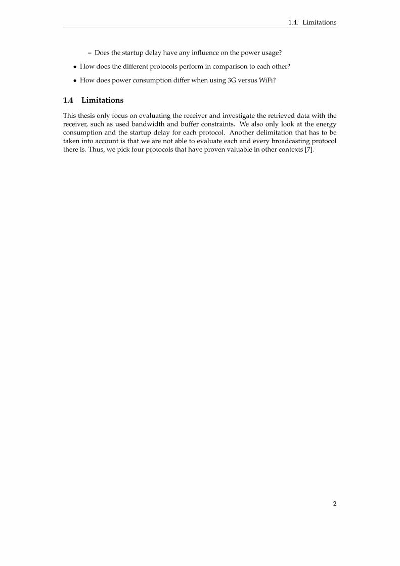
1.4 Limitations
This thesis only focus on evaluating the receiver and investigate the retrieved data with thereceiver, such as used bandwidth and buffer constraints. We also only look at the energyconsumption and the startup delay for each protocol. Another delimitation that has to betaken into account is that we are not able to evaluate each and every broadcasting protocolthere is. Thus, we pick four protocols that have proven valuable in other contexts [7].
2
2 Background
In this section we present some terms relevant to our thesis. We do not analyze each andevery protocol presented below, but the protocols are related to each other in one way oranother.
2.1 Broadcast
Broadcasting is a technology that allows one sender to deliver content to several mobile de-vices at once and could be used for sending live television through Long-Term Evolution(LTE) based mobile networks [11]. It is most easily understood as a technology that allowsyou to efficiently send from one sender to several receivers. Compared to traditional broad-cast used in Television distribution, these old systems might require up to three times theamount of frequency spectrum to cover the same area as a system broadcasted using theLTE network and more modern protocols. Starting with LTE, mobile networks has becomefast enough to handle high quality video transfers. This, combined with the fact that mod-ern protocols allows distributors to allocate frequencies dynamically has created these bigadvancements in frequency efficiency. If broadcasting is used today in LTE networks it ismostly using the same technique as traditional TV which means that all TV channels are al-locating their frequencies all the time even when no-one are watching them. In these casesthe advantages are minimised compared to more modern solutions as Evolved MultimediaBroadcast Multicast Services (eMBMS) which will only broadcast to channels that actuallygot viewers and allow the additional frequencies to be used for other purposes.
2.2 Multicast
Efficient information distribution is optimal during any scenario, making it important touse the correct protocol when it comes to disseminating information. Multicasting is aone-to-many or many-to-many distribution system that only sends data and information toreceivers who are listening for that specific information and if there are no-one listening, thedata is not transferred. Which is the main difference between broadcasting and multicasting.
When multicasting over LTE networks, using eMBMS is an efficient way to do so. eM-BMS is particularly efficient when the receiver has a temporary location and is often on the
3
2.3. Periodic Broadcast Protocol
move, e.g., mobile devices [4]. The most distinct difference between multicast and regularbroadcasting is that multicasting has intended receivers, while regular broadcasting sendsdata to anyone who listens to the transmission.
2.3 Periodic Broadcast Protocol
Periodic broadcast protocols [10] broadcasts videos periodically, meaning that a new streamis commenced every S minutes, where the video is transmitted from the host to the receiver.The interval in which the streams are started are called batching interval. This technique ofdata transmission is also called data centered because the server channels are dedicated to thedata that is being sent, rather then focusing on the user.
2.4 Pyramid Broadcasting
Pyramid broadcasting (PB) [10, 7, 15] was introduced in 1995 to reduce the service latencycreated by earlier periodic broadcast protocols. These earlier protocols broadcasts a videoevery batching interval, making increases in the server bandwidth the only way to improveservice latency.
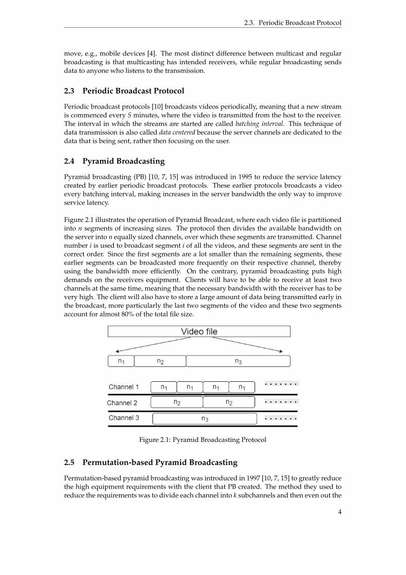
Figure 2.1 illustrates the operation of Pyramid Broadcast, where each video file is partitionedinto n segments of increasing sizes. The protocol then divides the available bandwidth onthe server into n equally sized channels, over which these segments are transmitted. Channelnumber i is used to broadcast segment i of all the videos, and these segments are sent in thecorrect order. Since the first segments are a lot smaller than the remaining segments, theseearlier segments can be broadcasted more frequently on their respective channel, therebyusing the bandwidth more efficiently. On the contrary, pyramid broadcasting puts highdemands on the receivers equipment. Clients will have to be able to receive at least twochannels at the same time, meaning that the necessary bandwidth with the receiver has to bevery high. The client will also have to store a large amount of data being transmitted early inthe broadcast, more particularly the last two segments of the video and these two segmentsaccount for almost 80% of the total file size.
Figure 2.1: Pyramid Broadcasting Protocol
2.5 Permutation-based Pyramid Broadcasting
Permutation-based pyramid broadcasting was introduced in 1997 [10, 7, 15] to greatly reducethe high equipment requirements with the client that PB created. The method they used toreduce the requirements was to divide each channel into k subchannels and then even out the
4
2.6. Optimized Periodic Broadcasting Protocol
starts of segments on these subchannels. By doing this they were able to prevent the clientfrom having to receive data from more than one channel at the time, and thereby reducingthe amount of bandwidth used by the client. This decrease in used bandwidth also led to adecrease in needed storage on the receiving unit, in fact just a third of the storage requiredwhen using PB.
2.6 Optimized Periodic Broadcasting Protocol
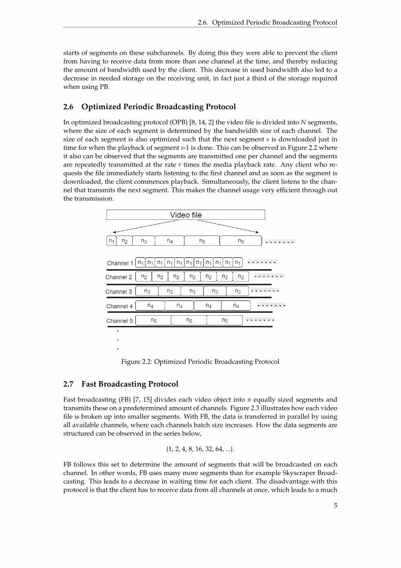
In optimized broadcasting protocol (OPB) [8, 14, 2] the video file is divided into N segments,where the size of each segment is determined by the bandwidth size of each channel. Thesize of each segment is also optimized such that the next segment s is downloaded just intime for when the playback of segment s-1 is done. This can be observed in Figure 2.2 whereit also can be observed that the segments are transmitted one per channel and the segmentsare repeatedly transmitted at the rate r times the media playback rate. Any client who re-quests the file immediately starts listening to the first channel and as soon as the segment isdownloaded, the client commences playback. Simultaneously, the client listens to the chan-nel that transmits the next segment. This makes the channel usage very efficient through outthe transmission.
Figure 2.2: Optimized Periodic Broadcasting Protocol
2.7 Fast Broadcasting Protocol
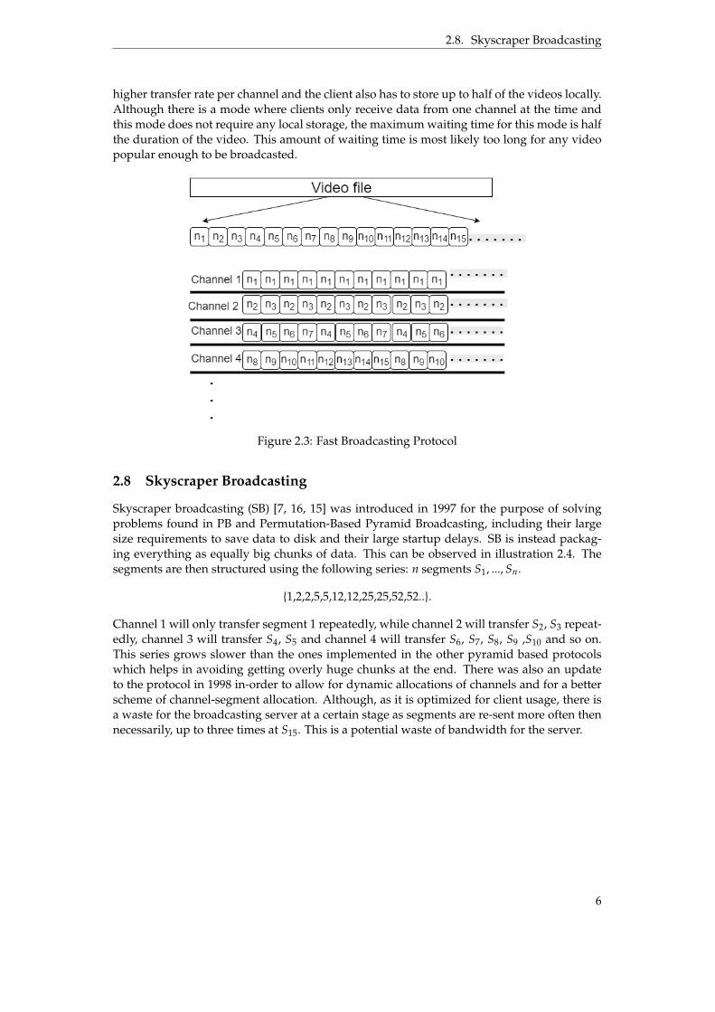
Fast broadcasting (FB) [7, 15] divides each video object into n equally sized segments andtransmits these on a predetermined amount of channels. Figure 2.3 illustrates how each videofile is broken up into smaller segments. With FB, the data is transferred in parallel by usingall available channels, where each channels batch size increases. How the data segments arestructured can be observed in the series below,
{1, 2, 4, 8, 16, 32, 64, ...}.
FB follows this set to determine the amount of segments that will be broadcasted on eachchannel. In other words, FB uses many more segments than for example Skyscraper Broad-casting. This leads to a decrease in waiting time for each client. The disadvantage with thisprotocol is that the client has to receive data from all channels at once, which leads to a much
5
2.8. Skyscraper Broadcasting
higher transfer rate per channel and the client also has to store up to half of the videos locally.Although there is a mode where clients only receive data from one channel at the time andthis mode does not require any local storage, the maximum waiting time for this mode is halfthe duration of the video. This amount of waiting time is most likely too long for any videopopular enough to be broadcasted.
Figure 2.3: Fast Broadcasting Protocol
2.8 Skyscraper Broadcasting
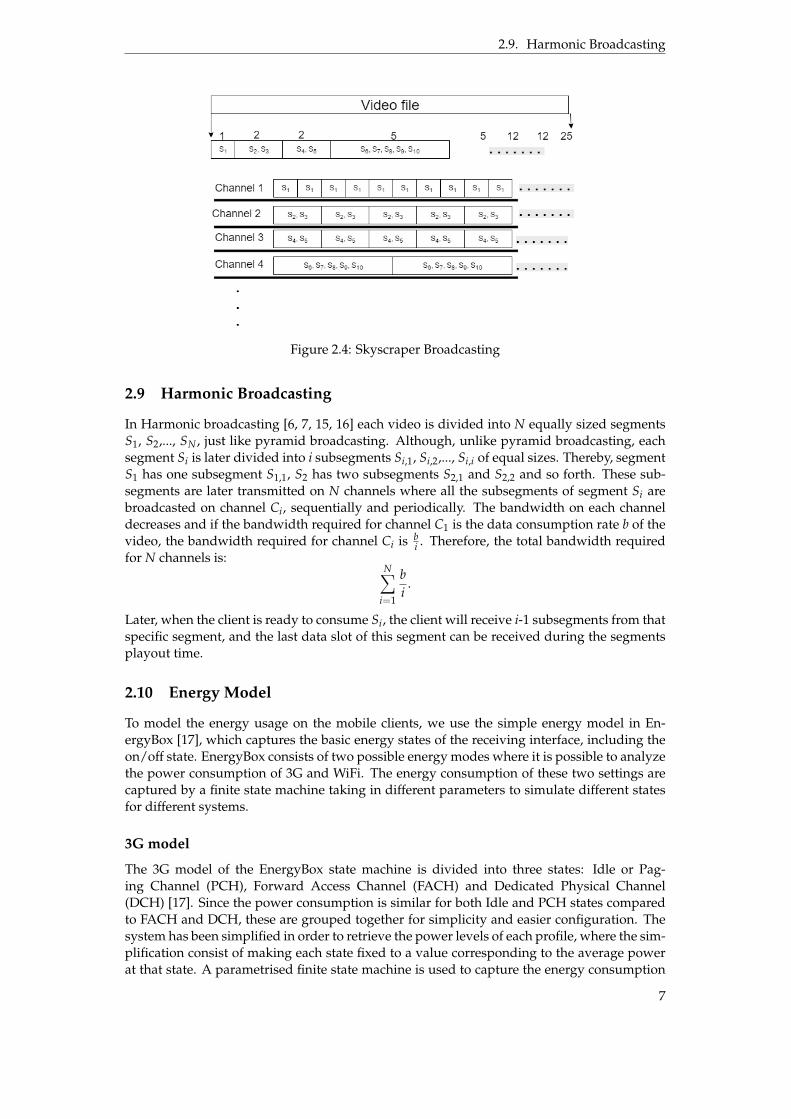
Skyscraper broadcasting (SB) [7, 16, 15] was introduced in 1997 for the purpose of solvingproblems found in PB and Permutation-Based Pyramid Broadcasting, including their largesize requirements to save data to disk and their large startup delays. SB is instead packag-ing everything as equally big chunks of data. This can be observed in illustration 2.4. Thesegments are then structured using the following series: n segments S1, ..., Sn.
{1,2,2,5,5,12,12,25,25,52,52..}.
Channel 1 will only transfer segment 1 repeatedly, while channel 2 will transfer S2, S3 repeat-edly, channel 3 will transfer S4, S5 and channel 4 will transfer S6, S7, S8, S9 ,S10 and so on.This series grows slower than the ones implemented in the other pyramid based protocolswhich helps in avoiding getting overly huge chunks at the end. There was also an updateto the protocol in 1998 in-order to allow for dynamic allocations of channels and for a betterscheme of channel-segment allocation. Although, as it is optimized for client usage, there isa waste for the broadcasting server at a certain stage as segments are re-sent more often thennecessarily, up to three times at S15. This is a potential waste of bandwidth for the server.
6
2.9. Harmonic Broadcasting
Figure 2.4: Skyscraper Broadcasting
2.9 Harmonic Broadcasting
In Harmonic broadcasting [6, 7, 15, 16] each video is divided into N equally sized segmentsS1, S2,..., SN , just like pyramid broadcasting. Although, unlike pyramid broadcasting, eachsegment Si is later divided into i subsegments Si,1, Si,2,..., Si,i of equal sizes. Thereby, segmentS1 has one subsegment S1,1, S2 has two subsegments S2,1 and S2,2 and so forth. These sub-segments are later transmitted on N channels where all the subsegments of segment Si arebroadcasted on channel Ci, sequentially and periodically. The bandwidth on each channeldecreases and if the bandwidth required for channel C1 is the data consumption rate b of thevideo, the bandwidth required for channel Ci is b
i . Therefore, the total bandwidth requiredfor N channels is:
Nÿ
i=1
b
i.
Later, when the client is ready to consume Si, the client will receive i-1 subsegments from thatspecific segment, and the last data slot of this segment can be received during the segmentsplayout time.
2.10 Energy Model
To model the energy usage on the mobile clients, we use the simple energy model in En-ergyBox [17], which captures the basic energy states of the receiving interface, including theon/off state. EnergyBox consists of two possible energy modes where it is possible to analyzethe power consumption of 3G and WiFi. The energy consumption of these two settings arecaptured by a finite state machine taking in different parameters to simulate different statesfor different systems.
3G model
The 3G model of the EnergyBox state machine is divided into three states: Idle or Pag-ing Channel (PCH), Forward Access Channel (FACH) and Dedicated Physical Channel(DCH) [17]. Since the power consumption is similar for both Idle and PCH states comparedto FACH and DCH, these are grouped together for simplicity and easier configuration. Thesystem has been simplified in order to retrieve the power levels of each profile, where the sim-plification consist of making each state fixed to a value corresponding to the average powerat that state. A parametrised finite state machine is used to capture the energy consumption
7

2.10. Energy Model
of 3G and to later simulate the inactivity timers, the Radio Link Control (RLC) buffers anda low activity mechanism, everything in a packet-driven manner. Figure 2.5(a) shows thestates of the 3G model and the state transitions we use in our simulations.
Figure 2.5: EnergyBox State Machine for 3G (a) and WiFi (b)
WiFi model
The WiFi mode in EnergyBox captures and measures the adaptive Power Save Mode (PSM)mechanism based on the amount of packets per second and on the inactivity timer [17]. Thestate machine shown in Figure 2.5(b) is used to model the data rate behaviour of a station,where the stations switch between two states, PSM and Constant Awake Mode (CAM), usingadaptive PSM. No data transmission is performed in the PSM state and the station only wakesup for beacons in this state. This state makes it possible for the station to switch to a lowpower mode when there is no data transferred. During the transmission interval there aresome station models that switch to a higher power, and it is in these models where the PSM-TX state represents the transmission of packets in the PSM mode. While the power savingfeatures are disabled the station is awake in CAM.
8
2.10. Energy Model
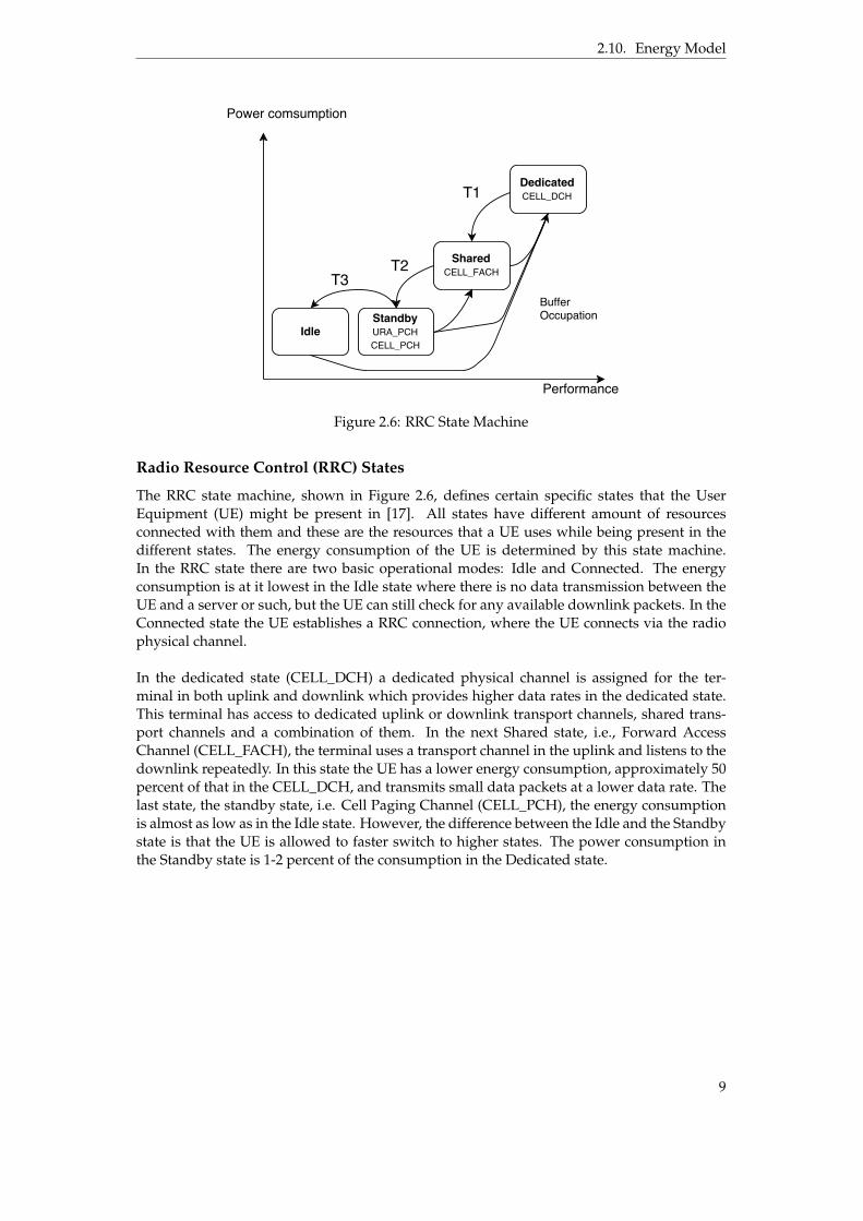
Figure 2.6: RRC State Machine
Radio Resource Control (RRC) States
The RRC state machine, shown in Figure 2.6, defines certain specific states that the UserEquipment (UE) might be present in [17]. All states have different amount of resourcesconnected with them and these are the resources that a UE uses while being present in thedifferent states. The energy consumption of the UE is determined by this state machine.In the RRC state there are two basic operational modes: Idle and Connected. The energyconsumption is at it lowest in the Idle state where there is no data transmission between theUE and a server or such, but the UE can still check for any available downlink packets. In theConnected state the UE establishes a RRC connection, where the UE connects via the radiophysical channel.
In the dedicated state (CELL_DCH) a dedicated physical channel is assigned for the ter-minal in both uplink and downlink which provides higher data rates in the dedicated state.This terminal has access to dedicated uplink or downlink transport channels, shared trans-port channels and a combination of them. In the next Shared state, i.e., Forward AccessChannel (CELL_FACH), the terminal uses a transport channel in the uplink and listens to thedownlink repeatedly. In this state the UE has a lower energy consumption, approximately 50percent of that in the CELL_DCH, and transmits small data packets at a lower data rate. Thelast state, the standby state, i.e. Cell Paging Channel (CELL_PCH), the energy consumptionis almost as low as in the Idle state. However, the difference between the Idle and the Standbystate is that the UE is allowed to faster switch to higher states. The power consumption inthe Standby state is 1-2 percent of the consumption in the Dedicated state.
9
3 Method
In order to measure how different protocols affects energy consumption in mobile devices,we have constructed a simulator for emulating packet transmissions during a multicastsession, while using one of our chosen broadcasting protocols. The protocols we have chosento simulate and analyze are PB, FB, OPB and SB.
Instead of analyzing real video transmission, our simulator broadcasts dummy User Data-gram Protocol (UDP) packets, imitating a real UDP-carrying video transmission. Thesetransmissions are then recorded with Wireshark. The recorded data is cleaned up so it justcontains packets related to the specific transmissions generated by the simulator. Theseare then analyzed using EnergyBox, to make an estimation of how long the mobile devicetransmitter has to be in the different transmissions states. This will result in the overall powerconsumed by the mobile units network components. Finally, the data from each protocolis compared and we analyze how each protocol behave when we change the values of ourinputs. These inputs include, the number of channels that the data are broadcasted through,the amount of bandwidth/bit rate on each channel, and the length of the video, wherevideo length and bit rate are kept the same for each measurement. This is done in order toevaluate the behaviours of the different protocols and if there is any significant difference inconsumption between them.
3.1 EnergyBox
EnergyBox is a tool developed at Linköpings University in order to measure power drainagein mobile devices when transmitting and retrieving data. The program takes a stored net-work session in the form of a pcap file and several different configuration files which itcombines in order to generate a estimation of the energy consumption that occurred whentransmitting the data found in the pcap file. EnergyBox takes real data traces creating realisticand reliable energy estimations.
Given a packet trace and some configuration parameters for EnergyBox, the program out-puts the devices states over time. These states are then associated with state-based powerlevels for a given device and later integrated over time, and this is how the total energy con-sumption is calculated. EnergyBox will be used to measure the energy consumption of our
10

3.2. Simulator
simulated protocols, creating graphs of the power usage and, to see how much time is spentin each state, as discussed earlier in Section 2.10. Figure 3.1 Illustrates generalization processof power usage profiles, and Appendix A presents example profiles from our examples.
Figure 3.1: EnergyBox [17]
3.2 Simulator
We have built a simulator to emulate the behaviours of the different protocols chosen forthis thesis. This software allows us to make customized schedules for the purpose of testingdifferent scenarios, on how fragmentation and channel usage behaves in different scenarios.This while also being able to generate schemes to emulate already established protocols suchas SB, PB, OPB and FB. The simulator is depending on inputs chosen by the user of thesimulator.
• Protocols: SB, PB, OBP, FBP are supported
• Channels: How many channels the simulator will use to transmit the data for the de-cided protocol.
• Bandwidth: This is converted to a bit rate.
• Video stream length: The length of the video stream in minutes.
• Playback Rate: How much faster the download rate is compared to playback rate.
• Sleep time: Time the simulator sleep between packet transmissions. If the sleep timeis set to 0 then the simulator pre-calculates a δ time to make every packet evenly dis-tributed over the transmission window. Otherwise, δ is the delay between packagetransmissions.
• Packet size: Size of each UDP packet in bytes that is to be transmitted.
SB can generate channel requirements depending on assigned bit rate and video length, wehave chosen to implement this support into the simulator as well. When having a predefinedamount of channels the simulator schedules fragments to the right channel and in the rightorder as decided by the chosen protocol. The output is when the channel is receiving data,when it is asleep, how many times the receiver was turned on and off and over how manysessions totally the channel was receiving data as-well as sleeping. In the final step thesimulator will emulate the traffic by sending shaped UDP packets on an available wirelessoutput device, simulating the transmission of our packet model. These transmissions aregenerated using a multi-threaded solution where each thread represents a channel that dur-ing a pre-calculated data timeframe transmits packages and during pre-calculated sleepingzones stops these packet transmissions. In the transmission phase the amount of packets totransmit are calculated by using the values of how many channels that are to be used, thestream length and the size of each packet. These total amount of packages will then be evenlydistributed between the transmission phases and transmitted when the simulator enters a
11

3.3. Wireshark
pre-calculated data session.
When transferring data there are two modes that can be used. The first is if sleep timeis set to zero, then the transmitter will pre-calculate the δ time between each sent package inorder to fill the entire data session as seen in Figure 3.2, the other way is to set a predefinedδ time to 1 - 2 ms. This will make the transmitter transmit data as fast as possible as seen inFigure 3.3 this effectively shortens transmit time making the resting time frame longer, thusshould result in some energy savings.
Figure 3.2: Even mode
Figure 3.3: Burst mode
3.3 Wireshark
Wireshark is a packet analyzer used for network troubleshooting, network analysis and com-munications protocol development. It has been used to record data generated by the simula-tor, as well as a tool for cleaning up the data from other types of packets that might have ar-rived during the simulated transmission, such as Internet Control Message Protocol (ICMP),Address Resolution Protocol (ARP) packets. This in order to make a trace clean from all otherunrelated network traffic, when we make the energy consumption calculation in Energybox.
3.4 Experiment and Design
The experiments are initiated by simulating the different protocols at two pre-determined bitrates, in order to evaluate how much impact a higher bitrate had on the energy consumption.The bit rate also had to be limited as EnergyBox had a hard time handling packet logs surpass-ing 30Mb. These restrictions lead to the choice of 500 kbit/s and 1000 kbit/s even if both ofthem are considered too low for a decent video-stream. EnergyBox is fed with configurationfiles made to emulate a mobile device "Nexus One" and a cellular 3G network "Telia" and theconfiguration for emulating an "Samsung G. S2" as receiver for our WiFi transmissions. Twocomputers will be used to generate the traffic, one that will be acting as a transmitter and onethat will act as an receiver. The receiving end will be using Wireshark and record all trans-mitted data. While the other is running our simulation software doing data transmissions.The test is replicated at each channel setup. The following raw data is generated.
• Data transmission are done simulating the following protocols PB, SB, FB, OPB usingour simulation software.
• Transmission uses two bit rates 500kbit/s and 1000kbit/s using even mode.
• Transmission for each protocol and bit rate setup are transmitted at 2, 3, 4, 6 and 8channels.
• Startup delay for each channel configuration is measured.
12
3.4. Experiment and Design
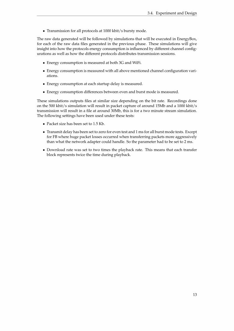
• Transmission for all protocols at 1000 kbit/s bursty mode.
The raw data generated will be followed by simulations that will be executed in EnergyBox,for each of the raw data files generated in the previous phase. These simulations will giveinsight into how the protocols energy consumption is influenced by different channel config-urations as well as how the different protocols distributes transmission sessions.
• Energy consumption is measured at both 3G and WiFi.
• Energy consumption is measured with all above mentioned channel configuration vari-ations.
• Energy consumption at each startup delay is measured.
• Energy consumption differences between even and burst mode is measured.
These simulations outputs files at similar size depending on the bit rate. Recordings doneon the 500 kbit/s simulation will result in packet capture of around 15Mb and a 1000 kbit/stransmission will result in a file at around 30Mb, this is for a two minute stream simulation.The following settings have been used under these tests:
• Packet size has been set to 1.5 Kb.
• Transmit delay has been set to zero for even test and 1 ms for all burst mode tests. Exceptfor FB where huge packet losses occurred when transferring packets more aggressivelythan what the network adapter could handle. So the parameter had to be set to 2 ms.
• Download rate was set to two times the playback rate. This means that each transferblock represents twice the time during playback.
13
4 Results
In this section we take a look at how different protocols behave compared to each other from aset of different variables. Such as energy consumption when using 3G or WiFi, how is evenlydistributed packages affecting energy consumption when compared to when receiving thempacked together in burst mode. Furthermore, how are more channels beneficial for bothenergy consumption and startup delay and how much energy is required before playback isachieved.
4.1 Pyramid Broadcasting
Energy consumption over channels
Tables 4.1 and 4.2 show the energy consumption for 3G and WiFi experiments, respectively.The results include scenarios when the data rates are 500kbit/s and 1000kbit/s, and caseswith both evenly distributed packages and when packages are sent in burst mode. Resultsare also summarized in Figures 4.1(b), 4.2(b) and 4.3. We note that the energy consumptionat the client is much lower when using WiFi than when using 3G. Both 3G plots show that theenergy usage is steadily increasing when we increased the amount of channels used, whentransmitting the data. While the energy usage is consistent when distributing the video usingWiFi, e.g., there is only a difference of approximately 2 Joule between the 2 channel simulationand the 8 channel simulation. We can see that when broadcasting over 8 channels the amountof energy consumed is almost doubled when using 3G compared to using WiFi. When com-paring energy consumption using evenly distributed packages and the ones received in burstmode, the power consumption is much reduced when using burst transmission compared toevenly distributed ones.
Startup delay over channels
Table 4.3 and Figures 4.1(a) and 4.2(a) show the startup delay for the transmissions, meaninghow much time it takes for the client before it is able to start watching a video. There is a majordecrease in startup delay when increasing the channels used from 2 to 4, and afterwards itdecreases in an even rate. The startup delay is very similar for both 500 kbit/s and 1000kbit/s, where the largest divergence is at the 2 channel distribution.
14

4.1. Pyramid Broadcasting
2 4 6 8
0
10
20
Channels
Sta
rtu
pD
elay
(sec
ond
s) 3G and WiFi
2 4 6 8
30
40
50
Channels
En
erg
yC
on
sum
pti
on
(Jou
le)
3GWiFi
Figure 4.1: Pyramid broadcasting 500 kbit/s, (a) Startup Delay, (b) Energy Consumption.
2 4 6 8
0
10
20
Channels
Sta
rtu
pD
elay
(sec
ond
s) 3G and WiFi
2 4 6 8
30
40
50
60
Channels
En
erg
yC
on
sum
pti
on
(Jou
le)
3GWiFi
Figure 4.2: Pyramid broadcasting 1000 kbit/s, (a) Startup Delay, (b) Energy Consumption.
2 4 6 810
20
30
Channels
En
erg
yC
on
sum
pti
on
(Jou
le)
WiFi EvenWiFi Burst
2 4 6 8
30
40
50
60
Channels
En
erg
yC
on
sum
pti
on
(Jou
le)
3G Even3G Burst
Figure 4.3: Pyramid broadcasting 1000 kbit/s. Even compared to Burst mode, (a) EnergyConsumption WiFi, (b) Energy Consumption 3G.
Energy consumption over startup delay
Figure 4.4 shows how much energy it takes to gain the startup delay that each transmissionhas over 2, 3, 4, 6 and 8 channels. As seen in the graphs it takes about 60 Joule to get a
15

4.2. Optimized Periodic Broadcasting
startup delay of roughly 0.4 seconds when transmitting over 8 channels. When decreasingthe amount of channels the energy consumed decreases as well, though the startup delayincreases greatly.
0 5 10 15 20
30
40
50
Startup Delay (seconds)
En
erg
yC
on
sum
pti
on
(Jou
le)
3GWiFi
0 5 10 15 20
30
40
50
60
Startup Delay (seconds)
En
erg
yC
on
sum
pti
on
(Jou
le)
3GWiFi
Figure 4.4: Pyramid broadcasting, (a) 500 kbit/s, (b) 1000 kbit/s.
Distribution Bit rate 2 channels 3 channels 4 channels 6 channels 8 channelsEven 500 kbit/s 47.74 52.02 53.90 55.97 57.13Even 1000 kbit/s 49.35 53.72 55.16 55.68 58.62Burst 1000 kbit/s 24.55 29.72 33.05 36.03 38.56
Table 4.1: Energy Consumption Pyramid broadcasting 3G
Distribution Bit rate 2 channels 3 channels 4 channels 6 channels 8 channelsEven 500 kbit/s 28.85 29.18 29.16 29.90 30.78Even 1000 kbit/s 30.19 30.63 30.29 30.09 32.27Burst 1000 kbit/s 12.00 12.47 12.52 12.99 14.67
Table 4.2: Energy Consumption Pyramid broadcasting WiFi
Bit rate 2 channels 3 channels 4 channels 6 channels 8 channels500 kbit/s 21.101 9.106 4.210 1.043 0.288
1000 kbit/s 22.463 9.589 4.389 1.085 0.356
Table 4.3: Startup Delay Pyramid broadcasting
4.2 Optimized Periodic Broadcasting
Energy consumption over channels
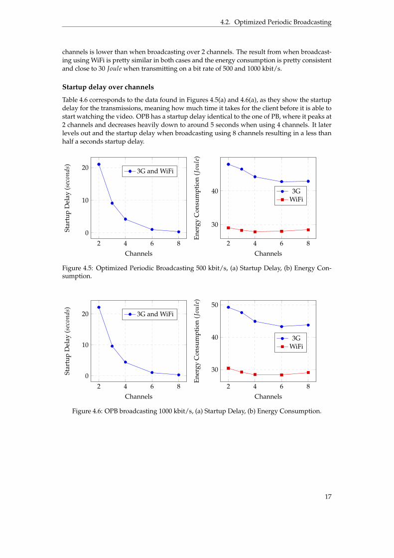
Tables 4.4 and 4.5 shows the energy consumption for 500kbit/s and 1000kbit/s for evenlydistributed packages and packages sent in burst mode. These data points corresponds to thedata shown in Figures 4.5, 4.6 and 4.7.The energy consumption with OPB differentiates slightly from the other protocols. Whenbroadcasting using 3G the energy usage reduces when increasing the amount of channelsused, for both 500 kbit/s and 1000 kbit/s. Furthermore, the energy consumed when using 8
16
4.2. Optimized Periodic Broadcasting
channels is lower than when broadcasting over 2 channels. The result from when broadcast-ing using WiFi is pretty similar in both cases and the energy consumption is pretty consistentand close to 30 Joule when transmitting on a bit rate of 500 and 1000 kbit/s.
Startup delay over channels
Table 4.6 corresponds to the data found in Figures 4.5(a) and 4.6(a), as they show the startupdelay for the transmissions, meaning how much time it takes for the client before it is able tostart watching the video. OPB has a startup delay identical to the one of PB, where it peaks at2 channels and decreases heavily down to around 5 seconds when using 4 channels. It laterlevels out and the startup delay when broadcasting using 8 channels resulting in a less thanhalf a seconds startup delay.
2 4 6 8
0
10
20
Channels
Sta
rtu
pD
elay
(sec
ond
s)
3G and WiFi
2 4 6 8
30
40
Channels
En
erg
yC
on
sum
pti
on
(Jou
le)
3GWiFi
Figure 4.5: Optimized Periodic Broadcasting 500 kbit/s, (a) Startup Delay, (b) Energy Con-sumption.
2 4 6 8
0
10
20
Channels
Sta
rtu
pD
elay
(sec
ond
s)
3G and WiFi
2 4 6 8
30
40
50
Channels
En
erg
yC
on
sum
pti
on
(Jou
le)
3GWiFi
Figure 4.6: OPB broadcasting 1000 kbit/s, (a) Startup Delay, (b) Energy Consumption.
17
4.2. Optimized Periodic Broadcasting
2 4 6 810
15
20
25
30
Channels
En
erg
yC
on
sum
pti
on
(Jou
le)
WiFi EvenWiFi Burst
2 4 6 8
30
40
50
Channels
En
erg
yC
on
sum
pti
on
(Jou
le)
3G Even3G Burst
Figure 4.7: Optimized Periodic Broadcasting 1000 kbit/s. Even compared to Burst mode, (a)Energy Consumption WiFi, (b) Energy Consumption 3G.
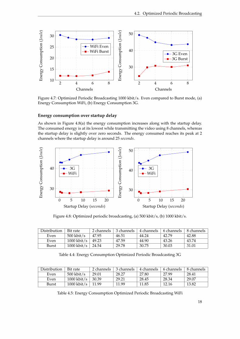
Energy consumption over startup delay
As shown in Figure 4.8(a) the energy consumption increases along with the startup delay.The consumed energy is at its lowest while transmitting the video using 8 channels, whereasthe startup delay is slightly over zero seconds. The energy consumed reaches its peak at 2channels where the startup delay is around 25 seconds.
0 5 10 15 20
30
40
Startup Delay (seconds)
En
erg
yC
on
sum
pti
on
(Jou
le)
3GWiFi
0 5 10 15 20
30
40
50
Startup Delay (seconds)
En
erg
yC
on
sum
pti
on
(Jou
le)
3GWiFi
Figure 4.8: Optimized periodic broadcasting, (a) 500 kbit/s, (b) 1000 kbit/s.
Distribution Bit rate 2 channels 3 channels 4 channels 6 channels 8 channelsEven 500 kbit/s 47.95 46.51 44.24 42.79 42.88Even 1000 kbit/s 49.23 47.59 44.90 43.26 43.74Burst 1000 kbit/s 24.54 29.78 30.75 30.03 31.01
Table 4.4: Energy Consumption Optimized Periodic Broadcasting 3G
Distribution Bit rate 2 channels 3 channels 4 channels 6 channels 8 channelsEven 500 kbit/s 29.01 28.27 27.80 27.99 28.41Even 1000 kbit/s 30.39 29.21 28.45 28.34 29.07Burst 1000 kbit/s 11.99 11.99 11.85 12.16 13.82
Table 4.5: Energy Consumption Optimized Periodic Broadcasting WiFi
18
4.3. Fast Broadcasting
Bit rate 2 channels 3 channels 4 channels 6 channels 8 channels500 kbit/s 21.001 9.093 4.201 1.033 0.289
1000 kbit/s 22.121 9.587 4.425 1.070 0.303
Table 4.6: Startup Delay Optimized Periodic Broadcasting
4.3 Fast Broadcasting
Energy consumption over channels
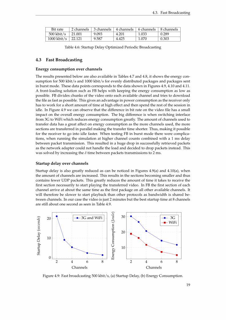
The results presented below are also available in Tables 4.7 and 4.8, it shows the energy con-sumption for 500 kbit/s and 1000 kbit/s for evenly distributed packages and packages sentin burst mode. These data points corresponds to the data shown in Figures 4.9, 4.10 and 4.11.A front-loading solution such as FB helps with keeping the energy consumption as low aspossible. FB divides chunks of the video onto each available channel and tries to downloadthe file as fast as possible. This gives an advantage in power consumption as the receiver onlyhas to work for a short amount of time at high effect and then spend the rest of the session inidle. In Figure 4.9 we can observe that the difference in bit rate on the video file has a smallimpact on the overall energy consumption. The big difference is when switching interfacefrom 3G to WiFi which reduces energy consumption greatly. The amount of channels used totransfer data has a great affect on energy consumption as the more channels used, the moresections are transferred in parallel making the transfer time shorter. Thus, making it possiblefor the receiver to go into idle faster. When testing FB in burst mode there were complica-tions, when running the simulation at higher channel counts combined with a 1 ms delaybetween packet transmission. This resulted in a huge drop in successfully retrieved packetsas the network adapter could not handle the load and decided to drop packets instead. Thiswas solved by increasing the δ time between packets transmissions to 2 ms.
Startup delay over channels
Startup delay is also greatly reduced as can be noticed in Figures 4.9(a) and 4.10(a), whenthe amount of channels are increased. This results in the sections becoming smaller and thuscontains fewer UDP packets. This greatly reduces the amount of time it takes to receive thefirst section necessarily to start playing the transferred video. In FB the first section of eachchannel arrive at about the same time as the first package on all other available channels. Itwill therefore be slower to start playback than other protocols as bandwidth is shared be-tween channels. In our case the video is just 2 minutes but the best startup time at 8 channelsare still about one second as seen in Table 4.9.
2 4 6 80
10
20
Channels
Sta
rtu
pD
elay
(sec
ond
s) 3G and WiFi
2 4 6 8
10
20
30
Channels
En
erg
yC
on
sum
pti
on
(Jou
le)
3GWiFi
Figure 4.9: Fast broadcasting 500 kbit/s, (a) Startup Delay, (b) Energy Consumption.
19

4.3. Fast Broadcasting
2 4 6 80
10
20
Channels
Sta
rtu
pD
elay
(sec
ond
s) 3G and WiFi
2 4 6 8
10
20
30
Channels
En
erg
yC
on
sum
pti
on
(Jou
le)
3GWiFi
Figure 4.10: Fast broadcasting 1000 kbit/s, (a) Startup Delay, (b) Energy Consumption.
2 4 6 8
5
10
15
20
Channels
En
erg
yC
on
sum
pti
on
(Jou
le)
WiFi EvenWiFi Burst
2 4 6 8
10
20
30
Channels
En
erg
yC
on
sum
pti
on
(Jou
le)
3G Even3G Burst
Figure 4.11: Fast broadcasting 1000 kbit/s Even compared to Burst mode, (a) Energy Con-sumption WiFi, (b) Energy Consumption 3G.
Energy consumption over startup delay
Energy consumption before having the first section completely downloaded are greatly re-duced as more channels are used. It can bee seen in Figure 4.12 that the longer the user haveto wait in order to get the first section, the higher the power consumption for getting the firstsection will be.
20

4.4. Skyscraper Broadcasting
0 5 10 15 20
10
20
30
Startup Delay (seconds)
En
erg
yC
on
sum
pti
on
(Jou
le)
3GWiFi
0 5 10 15 20
10
20
30
Startup Delay (seconds)
En
erg
yC
on
sum
pti
on
(Jou
le)
3GWiFi
Figure 4.12: Fast broadcasting, (a) 500 kbit/s, (b) 1000 kbit/s.
Distribution Bit rate 2 channels 3 channels 4 channels 6 channels 8 channelsEven 500 kbit/s 30.22 26.55 20.68 14.45 11.76Even 1000 kbit/s 31.42 27.63 21.33 14.76 11.97Burst 1000 kbit/s 22.90 20.39 15.98 11.65 9.73
Table 4.7: Energy Consumption Fast broadcasting 3G
Distribution Bit rate 2 channels 3 channels 4 channels 6 channels 8 channelsEven 500 kbit/s 18.90 16.23 11.80 7.15 5.14Even 1000 kbit/s 19.83 17.03 12.30 7.38 5.30Burst 1000 kbit/s 13.49 11.61 8.30 5.05 3.61
Table 4.8: Energy Consumption Fast broadcasting WiFi
Bit rate 2 channels 3 channels 4 channels 6 channels 8 channels500 kbit/s 21.112 9.028 5.260 2.279 1.262
1000 kbit/s 22.246 9.555 5.435 2.422 1.308
Table 4.9: Startup Delay Fast broadcasting
4.4 Skyscraper Broadcasting
Energy consumption over channels
As seen in Tables 4.10 and 4.11 the energy consumption is shown for transmission rates of500kbit/s and 1000kbit/s, and for both evenly distributed packages and packages sent inburst mode. These data points corresponds to the data shown in Figures 4.13(b), 4.14(b)and 4.15(b). The energy consumption when switching from 500 kbit/s to 1000 kbit/s in-creases faster as channels are added, but the growth evens out as it reaches the peek of 8channels. At two channels the consumption is lower but not capable of competing with mostother protocols. SB increases segment length as more channels are added and this forces thereceiver to stay on for a longer time with each added channel, which can be seen in Tables 4.10and 4.11. When measuring the consumption on WiFi we can see in energy figures that theenergy consumption starts at a much lower level and keeps growing much slower than the3G simulation.
21
4.4. Skyscraper Broadcasting
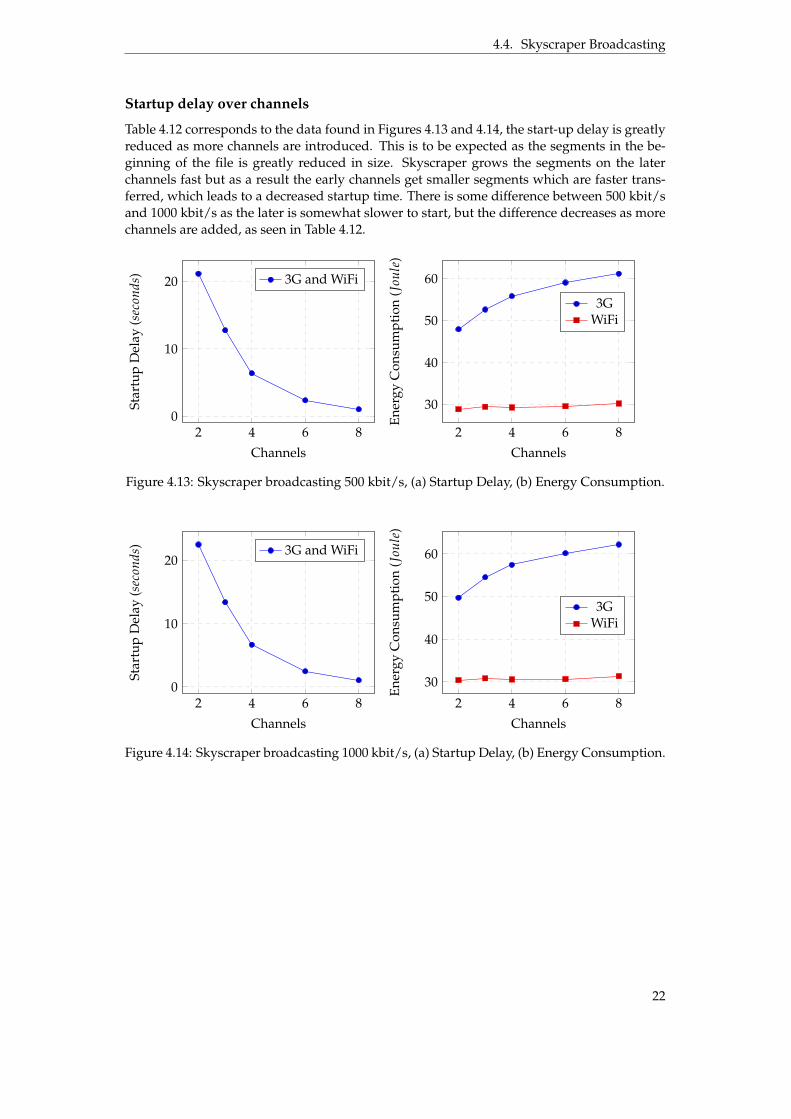
Startup delay over channels
Table 4.12 corresponds to the data found in Figures 4.13 and 4.14, the start-up delay is greatlyreduced as more channels are introduced. This is to be expected as the segments in the be-ginning of the file is greatly reduced in size. Skyscraper grows the segments on the laterchannels fast but as a result the early channels get smaller segments which are faster trans-ferred, which leads to a decreased startup time. There is some difference between 500 kbit/sand 1000 kbit/s as the later is somewhat slower to start, but the difference decreases as morechannels are added, as seen in Table 4.12.
2 4 6 80
10
20
Channels
Sta
rtu
pD
elay
(sec
ond
s) 3G and WiFi
2 4 6 8
30
40
50
60
Channels
En
erg
yC
on
sum
pti
on
(Jou
le)
3GWiFi
Figure 4.13: Skyscraper broadcasting 500 kbit/s, (a) Startup Delay, (b) Energy Consumption.
2 4 6 80
10
20
Channels
Sta
rtu
pD
elay
(sec
ond
s) 3G and WiFi
2 4 6 8
30
40
50
60
Channels
En
erg
yC
on
sum
pti
on
(Jou
le)
3GWiFi
Figure 4.14: Skyscraper broadcasting 1000 kbit/s, (a) Startup Delay, (b) Energy Consumption.
22
4.4. Skyscraper Broadcasting
2 4 6 8
20
30
Channels
En
erg
yC
on
sum
pti
on
(Jou
le)
WiFi EvenWiFi Burst
2 4 6 8
40
60
Channels
En
erg
yC
on
sum
pti
on
(Jou
le)
3G Even3G Burst
Figure 4.15: SkyScraper broadcasting 1000 kbit/s Even compared to Burst mode, (a) EnergyConsumption WiFi, (b) Energy Consumption 3G.
Energy consumption over startup delay
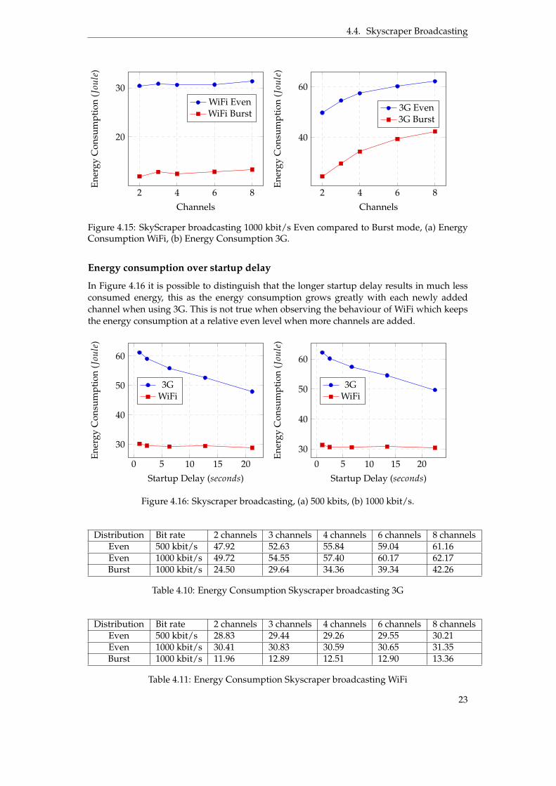
In Figure 4.16 it is possible to distinguish that the longer startup delay results in much lessconsumed energy, this as the energy consumption grows greatly with each newly addedchannel when using 3G. This is not true when observing the behaviour of WiFi which keepsthe energy consumption at a relative even level when more channels are added.
0 5 10 15 20
30
40
50
60
Startup Delay (seconds)
En
erg
yC
on
sum
pti
on
(Jou
le)
3GWiFi
0 5 10 15 20
30
40
50
60
Startup Delay (seconds)
En
erg
yC
on
sum
pti
on
(Jou
le)
3GWiFi
Figure 4.16: Skyscraper broadcasting, (a) 500 kbits, (b) 1000 kbit/s.
Distribution Bit rate 2 channels 3 channels 4 channels 6 channels 8 channelsEven 500 kbit/s 47.92 52.63 55.84 59.04 61.16Even 1000 kbit/s 49.72 54.55 57.40 60.17 62.17Burst 1000 kbit/s 24.50 29.64 34.36 39.34 42.26
Table 4.10: Energy Consumption Skyscraper broadcasting 3G
Distribution Bit rate 2 channels 3 channels 4 channels 6 channels 8 channelsEven 500 kbit/s 28.83 29.44 29.26 29.55 30.21Even 1000 kbit/s 30.41 30.83 30.59 30.65 31.35Burst 1000 kbit/s 11.96 12.89 12.51 12.90 13.36
Table 4.11: Energy Consumption Skyscraper broadcasting WiFi
23
4.5. Protocol Comparison
Bit rate 2 channels 3 channels 4 channels 6 channels 8 channels500 kbit/s 21.139 12.746 6.374 2.357 1.025
1000 kbit/s 22.485 13.389 6.667 2.475 1.071
Table 4.12: Startup Delay Skyscraper broadcasting
4.5 Protocol Comparison
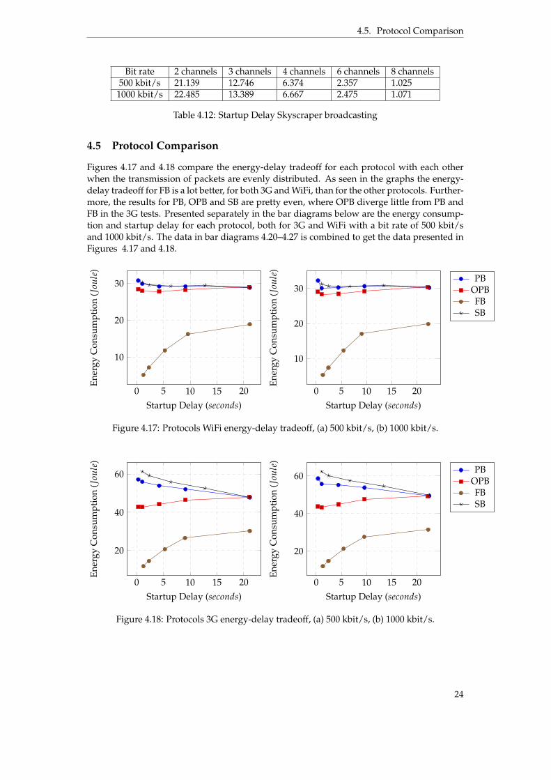
Figures 4.17 and 4.18 compare the energy-delay tradeoff for each protocol with each otherwhen the transmission of packets are evenly distributed. As seen in the graphs the energy-delay tradeoff for FB is a lot better, for both 3G and WiFi, than for the other protocols. Further-more, the results for PB, OPB and SB are pretty even, where OPB diverge little from PB andFB in the 3G tests. Presented separately in the bar diagrams below are the energy consump-tion and startup delay for each protocol, both for 3G and WiFi with a bit rate of 500 kbit/sand 1000 kbit/s. The data in bar diagrams 4.20–4.27 is combined to get the data presented inFigures 4.17 and 4.18.
0 5 10 15 20
10
20
30
Startup Delay (seconds)
En
erg
yC
on
sum
pti
on
(Jou
le)
0 5 10 15 20
10
20
30
Startup Delay (seconds)
En
erg
yC
on
sum
pti
on
(Jou
le)
PBOPBFBSB
Figure 4.17: Protocols WiFi energy-delay tradeoff, (a) 500 kbit/s, (b) 1000 kbit/s.
0 5 10 15 20
20
40
60
Startup Delay (seconds)
En
erg
yC
on
sum
pti
on
(Jou
le)
0 5 10 15 20
20
40
60
Startup Delay (seconds)
En
erg
yC
on
sum
pti
on
(Jou
le)
PBOPBFBSB
Figure 4.18: Protocols 3G energy-delay tradeoff, (a) 500 kbit/s, (b) 1000 kbit/s.
24
4.5. Protocol Comparison
0 5 10 15 20
10
20
30
40
Startup Delay (seconds)
En
erg
yC
on
sum
pti
on
(Jou
le)
0 5 10 15 20
5
10
15
Startup Delay (seconds)
En
erg
yC
on
sum
pti
on
(Jou
le)
PBOPBFBSB
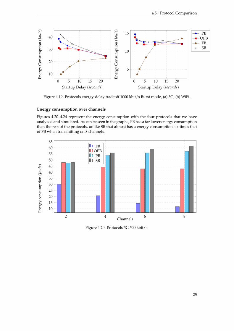
Figure 4.19: Protocols energy-delay tradeoff 1000 kbit/s Burst mode, (a) 3G, (b) WiFi.
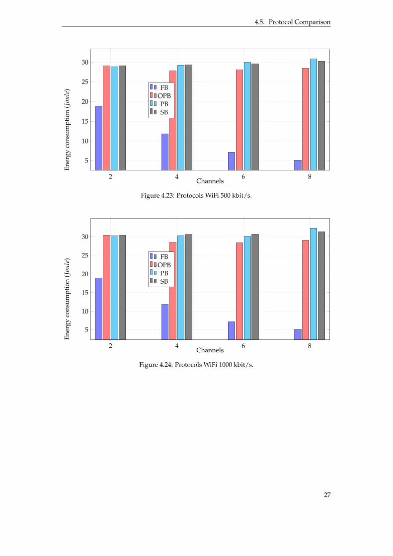
Energy consumption over channels
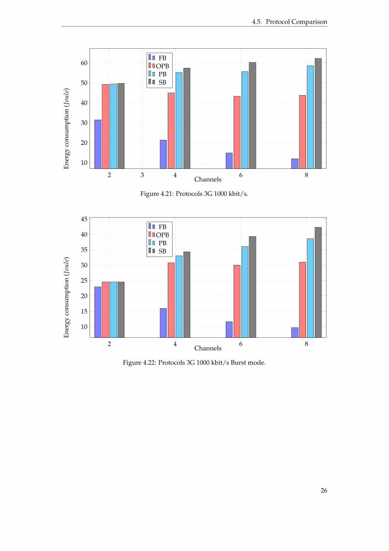
Figures 4.20–4.24 represent the energy consumption with the four protocols that we haveanalyzed and simulated. As can be seen in the graphs, FB has a far lower energy consumptionthan the rest of the protocols, unlike SB that almost has a energy consumption six times thatof FB when transmitting on 8 channels.
2 4 6 8
10
15
20
25
30
35
40
45
50
55
60
65
Channels
En
erg
yco
nsu
mp
tio
n(J
oule
)
FBOPBPBSB
Figure 4.20: Protocols 3G 500 kbit/s.
25
4.5. Protocol Comparison
2 3 4 6 8
10
20
30
40
50
60
Channels
En
erg
yco
nsu
mp
tio
n(J
oule
)FB
OPBPBSB
Figure 4.21: Protocols 3G 1000 kbit/s.
2 4 6 8
10
15
20
25
30
35
40
45
Channels
En
erg
yco
nsu
mp
tio
n(J
oule
)
FBOPBPBSB
Figure 4.22: Protocols 3G 1000 kbit/s Burst mode.
26
4.5. Protocol Comparison
2 4 6 8
5
10
15
20
25
30
Channels
En
erg
yco
nsu
mp
tio
n(J
oule
) FBOPBPBSB
Figure 4.23: Protocols WiFi 500 kbit/s.
2 4 6 8
5
10
15
20
25
30
Channels
En
erg
yco
nsu
mp
tio
n(J
oule
) FBOPBPBSB
Figure 4.24: Protocols WiFi 1000 kbit/s.
27

4.5. Protocol Comparison
2 4 6 8
4
6
8
10
12
14
Channels
En
erg
yco
nsu
mp
tio
n(J
oule
)FB
OPBPBSB
Figure 4.25: Protocols WiFi 1000 kbit/s Burst mode.
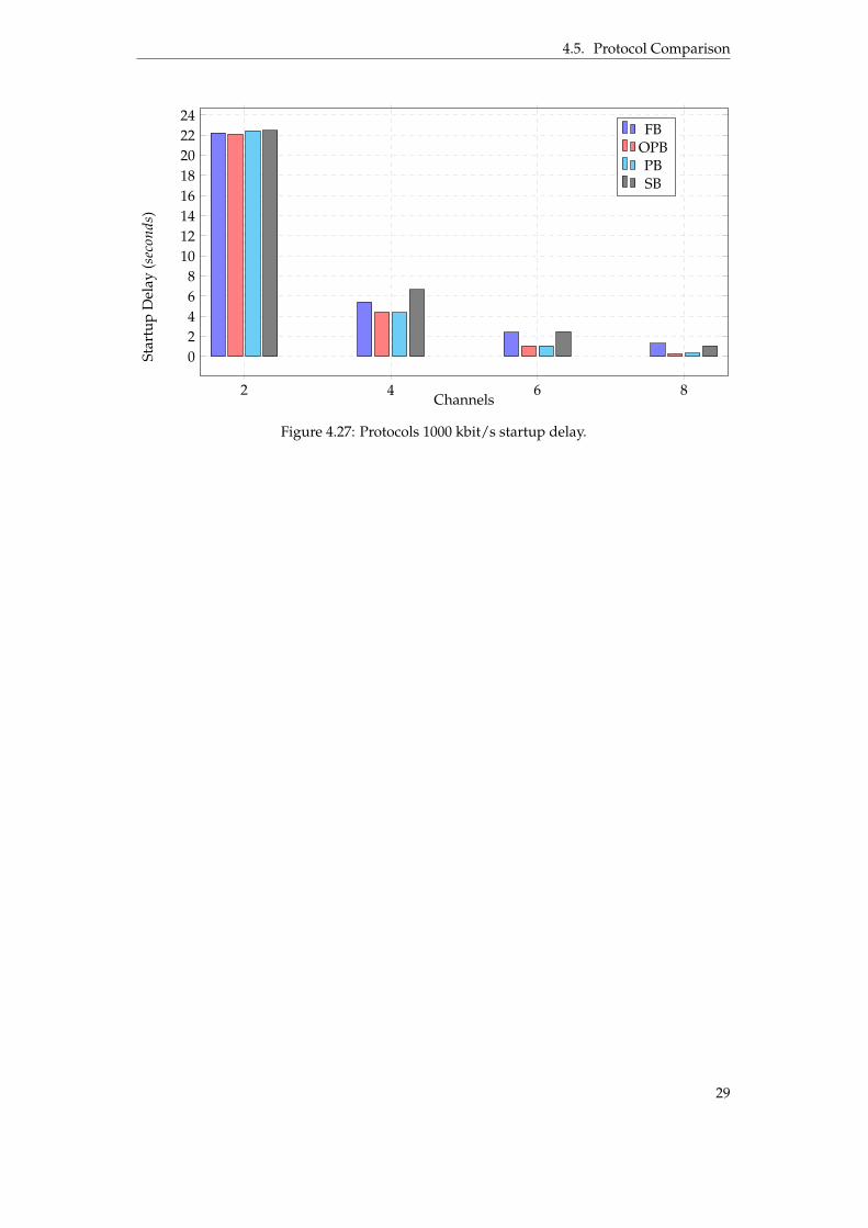
Startup delay over channels
Figures 4.26 and 4.27 shows that more channels reduces start up time greatly on all protocolswith no exception. This is as expected as early segments gets smaller with more channels.The ones taking the most benefit is OPB and PB as their earlier segments shrink faster thanthe others. When using just 2 channels the difference between protocols are almost negligiblebut when we reach 4 channels the gains are huge and when 8 channels are reached some arehaving startup times within less than one second, which could be considered good since thesimulated video is 2 minutes long.
2 4 6 8
0
2
4
6
8
10
12
14
16
18
20
22
Channels
Sta
rtu
pD
elay
(sec
ond
s)
FBOPBPBSB
Figure 4.26: Protocols 500 kbit/s startup delay.
28
4.5. Protocol Comparison
2 4 6 8
0
2
4
6
8
10
12
14
16
18
20
22
24
Channels
Sta
rtu
pD
elay
(sec
ond
s)FB
OPBPBSB
Figure 4.27: Protocols 1000 kbit/s startup delay.
29

5 Discussion
In this chapter we mainly discuss the two major parts of this thesis, the result and the method-ology. However, we also address some of the limitations we have taken into account and howthese have influenced our work.We also refer to figures found in the Appendix(numbered as A.X, where X is the figure num-ber within the Appendix).
5.1 Limitations
The first restriction we did was to decide upon how many protocols we wanted to workwith. There was not enough time to evaluate each and every broadcasting protocol, so wedecided to evaluate four that we found interesting. Thus, limiting both our study and ourresults. Even though we got a clear result of which protocol, of the ones we studied, is thebest when it comes to saving energy on a receiving device the study could be expanded toevaluating more protocols.Another delimitation we decided upon before we began this study was to only analyze thereceiver and how the data transmission affected the energy consumed with the end client. Wedecided on this approach because we found it more interesting and more important to havea knowledge about how to optimize a data transmission from the end users point-of-view.
All limitations were not decided upon starting this thesis. There were also several onesthat had to be taken into account as we encountered problems that forced us to change ourapproach. For example we encountered that EnergyBox had a limit on how large the fileswere allowed to be for EnergyBox to process them. This had us restricting our video file totwo minutes as well as keeping the bit rate bellow 1200 kbit/s.
5.2 Results
Quite a few results turned out as expected. The preliminary belief was that a front loadingprotocol would get advantages as it is more efficient to transfer data as fast as possible andthen turn off the receiver entirely, than to spread it out and keep the receiver working for alonger time. Additional tests were done here to further test this. This is where we simulated
30
5.2. Results
to transmit packages in bursts, meaning that we tried to transfer them as fast as possible inall transfer windows in-order to let the receiver start resting even within the transfer windowitself. The other testing states were done to evenly distribute the packages, with the theorythat if few enough packages were to be received after each other, the system would revert toa lower energy state, as too few packages were transmitted thus not breaking the thresholdkeeping the receiver in the DCH state.
Fast Broadcasting
FB were believed to be very efficient from the start, it were also expected that it would gaingreatly from additional channels as it is capable of downloading segments faster, the morechannels it get available. In Figure A.6 it is possible to distinguish from the graph that thedownload rate makes the receiver go into the DCH state and when the requests stops it staysthere for a while before going down to FACH. This behaviour can be found in all figuresrepresenting Fast broadcasting’s states. The device will stay in FACH for a predeterminedtime and will therefore always be the same, the same applies for the higher power level DCH,where it will stay a while after the last request has been received before stepping down.In FB this is used efficiently as most packages can be transmitted during very few transferwindows, this is where the receiver is fully active. It were even further improved upon whenallowing it to send packages in bursts, this as multiple channels are transmitting in parallelwhilst the receiver keeps active in DCH state with very short delays between the packages.As it transfers everything fast it can then quickly allow the receiver to go down to PCH/Idleagain. An increase in channels transmitting parallel greatly reduced start up delay as-well asit is using the receiver more efficiently. But the downsides are that it could never get closeto the startup times like some of the other protocols tested in this thesis and as the videowe simulated was only 2 minutes long. This could become annoying if the video were tobe longer than the one simulated in this test, which is most likely the case for most real lifeapplications.
Pyramid Broadcasting
PB were one of the highest power consumers and it kept growing as more channels wereadded, especially bad is it when the transmission are done at 3G where the energy consumedraises aggressively, as can be seen in Figure 4.1. This is most likely due to the receiver neverbeing able to go down to PCH/Idle. When the amount of channels are increased so are thespread of the DCH states. PB is spreading its sections very well due to how it is constructed.When one section is done the receiver starts to download the next one on a different channel.As the sections are not ever overlapping the efficient usage of the receiver becomes poor.This were much improved upon when making use of bursts instead, allowing the receiverto step down from DCH to FACH and even PCH. If A.13 and A.15 are compared it can bedistinguished that the time the receiver is allowed to stay in PCH/Idle is greatly increased,the same results can be found when analyzing A.14 and A.16 where the transmission at 8channels had almost no opportunity in wide mode to reach the lower power levels, whichwere changed when allowing burst mode. The power savings in this case where close to 20Joule which is a reduction of 35% which can be considered a quite good improvement. PBbenefits greatly from having more channels when observing the start up delay, this as it isgrowing it’s sections very fast and thus making the earlier ones very small. Which is goodwhen you want to get the playback going as fast as possible. Taking a look at Table 4.3 it canbe noticed that it is having one of the best start up times of all the protocols this thesis haveconducted tests upon and when working over WiFi, the energy consumption is acceptable.The question would be on how much more channels would decrease start up delay and howmuch the power consumption would increase as a result.
31

5.2. Results
Skyscraper Broadcasting
SB is also among these high consumers, as the energy consumption grows fast with moreadded channels especially on 3G. It keeps around PB levels of power consumption when run-ning over WiFi. This could be explained in Figure A.10 where the power states are changingoften between DCH, FACH and PCH. The more channels that are added the more time theprotocol spends in DCH, as can be seen in Figure 4.13 this greatly increases power consump-tion. At lower channel counts the receiver actually get to rest and powers down to PCH/Idlewhich is why fewer channels actually are consuming less power. This is greatly improvedupon when running in burst mode, allowing everything to get done as soon as possible andthe amount of time spent in PCH/Idle is therefore greatly increased as seen in A.9 where it isspread over the transmission window, and A.11 where it is transmitting as fast as possible on2 channels. When analyzing the 8 channel configuration it can be noticed that in A.10 thereis almost no PCH/Idle occurring at all and at most cases the receiver is not allowed to stepfurther down than the FACH stage. This is changed a great deal when looking at the samechannel configuration again but instead with using burst mode A.12. As seen in the graph thereceiver is able to not only reach FACH but also PCH/Idle. Therefore reducing the consumedpower from around 61.2 Joule to approximately 42.3 Joule. Reducing the energy consumedby approximately 18 Joule, which is an improvement of about 31%. Indicating that sendingdata as fast as possible is greatly advantageous.A higher amount of channels helps getting the startup delay down, but it is still the worstcompetitor in this test. When comparing the startup delay between protocols it shows quitebad results with only FB getting worse results in this test. SB grows slower than PB as a resultof its design. It will therefore require much more channels in order to get the earlier sectionssmall enough to be transferred within a reasonable timeframe.
Optimized Pyramid Broadcasting
OPB is giving quite different results when comparing the 500 kbit/s and 1000 bkit/s, seeTables 4.5 and 4.6. At 2 channels at 500 kbit/s, OPB gets to rest between the DCH states asfewer requests results in it being able to reach the FACH state. Which should explain why it isconsuming less power than the ones using more channels. When using 8 channels we get an-other dip in power consumption and this could be related to that the receiver gets everythingdone in one go. As seen in Figure A.2, this is similar to the behaviour of FB which would ex-plain the reduced power drainage as the transfer time is reduced. It should be noted that fourchannels have a disadvantage caused by the built in delay feature in 3G data transmissions.This resulting in the receiver not being able to step down to FACH as the gaps between trans-missions are shorter than the timeout for changing energy state. When the receiver enters aresting window, its shorter then the timeout so it stays in DCH for the entire session, evenwhen not sending data as seen in previous figures. This is much improved upon when run-ning OPB in burst mode instead as seen in Figure A.4. The advantage gets even more obviouswhen comparing Figure A.1 and A.3 where the advantage in energy consumption betweenthe 8 channel configurations goes from 29.1 Joule when evenly distributed to 13.8 Joule whentransmitting in bursts. This is a difference of about 15.3 joule giving a 53% advantage, whichis the biggest gain of all protocols when switching in between evenly distributed and burstdistributed transmissions.When observing the startup delay it is obvious that OPB is very good at delivering the firstsession fast as the startup delay is very low which can be observed in Table 4.9. This getsbetter as more channels are added resulting in one of the lowest startup delays in this test.When looking at energy consumption compared to startup delay we notice that it comes witha cost as longer startup delay in this case results in lower power consumption.
32

5.2. Results
Protocol Comparison
When comparing the tested protocols with each other we find that from an energy per-spective, FB is the one with the lowest energy consumption and OPB is the one with theshortest startup delay. This can be seen easily in Figures 4.20 and 4.21, the difference isobvious when analyzing the WiFi graphs as most are keeping themselves around the sameenergy consumption levels except for FB which gains a lot by the WiFi interface as seen inFigures 4.23 and 4.24. When taking these values and comparing them to the ones generatedwhen receiving data in bursts, the energy consumption shrinks quite distinctively but itis still FB which is the one consuming the least amount of power as seen in Figure 4.22.The advantage has shrunken as both Pyramid and Skyscraper were consuming about 30%more energy when transmission where evenly distributed compared to the ones transmittedin bursts. OPB makes a great gain as it was consuming approximately 50% more whentransmission where evenly distributed. When comparing the consumption using WiFi evengreater benefits can be found as most protocols are consuming about 50% more when evenlydistributed, except for FB as its gains are planning out. We expect that FB is reaching a lowerbound on consumption, it might be reduced somewhat more if more channels where to beadded but not with as much gains as earlier reductions. When analyzing startup delay it isOPB and PB who are the winners as both FB and SB do not keep up as more channels areadded which can be seen in Figures 4.26 and 4.27. In our simulation there were also no gainsin startup delay when using burst as the simulator only declared transmission completewhen the transmission window where over which in bursts case would occur a while afterthe actual data transmission were completed.
In Figures 4.17 and 4.18 there is a comparison for how energy consumption related tostartup delay behaves for all protocols. As earlier discussed FB got a big advantage over theentire range of channels. This advantage grows fast compared to the other protocols whohave a more modest gain. This is of course because of the heavy front loading, where FBgets more done whenever activating the receiver. There are also some gains for OPB as morechannels are added with a small peak at 6 channels, this behaviour can be found in the resultfor both 3G and WiFi. If additional channels where to be added our theory is that energyconsumption will continue to rise. In both SB and PB a rise of consumption can be observedas additional channels are added, this is caused by how it is distributing packages over thetransmission windows.In Figure 4.19 similar results can be observed as in Figures 4.17 and 4.18, but burst mode givesan advantage in energy consumption related to shorter transmission windows. This givesthe graphs the same behaviour, but the energy consumed is much lower when transmittingdata using burst mode.
Ranking of protocols
Table 5.1 presents a ranking of all the protocols, and how they are ranked relative to eachother. FB has so low energy consumption that even with the worst startup delay it still man-ages to come out on top, the same when we compare energy given bandwidth. Howeverwhen comparing startup delay and bandwidth OPB is superior to the other protocols. FBhave the worst startup delay of all the protocols and is therefore ranked last. Otherwise OPBreaches the second spot in two out of three tables, this combined with its low startup timemakes OPB quite good for all-round usage. OPB have the best startup time as well as thelowest buffer. In some cases it is difficult to order SB and PB relative to each other. To seethis, note that they typically operate in different ends of the tradeoff spectrum. For example,SB has a very high startup time and a low buffer requirements, whereas PB has very shortstartup times but require much smaller buffers. With regards to startup times, FB ranks as
33

5.3. Method
the worst as it both is the slowest starter combined with being the protocol that requires themost data being buffered, as everything is downloaded in parallel.
Comparison Rank 1 Rank 2 Rank 3 Rank 4Energy, givenstartup delay
FB OPB PB/SB PB/SB
Energy, givenbandwidth
FB OPB PB SB
Startup delay,given bandwidth
OPB PB SB FB
Buffer, givenenergy
OPB FB PB/SB PB/SB
Buffer, givenbandwidth
OPB FB SB PB
Buffer, givenstartup delay
OPB SB PB FB
Table 5.1: Ranking of protocols
5.3 Method
The method used is measurement and data driven. A simulator have been theorized andcoded, and this simulator have been used to simulate large streams of data packets imitatingreal time video traffic, these datas have then been analyzed. To capture the data transmissionwe used the tool Wireshark presented in Section 3.3 and later analyzed this data using Ener-gyBox presented in Section 3.1.
Even though we are satisfied with our result and think that the thesis is reliable, a wayto get a more reliable result could be to analyze larger data files as the bit rates that wasanalyzed in this thesis is much lower than what can be anticipated in real-life applications.However, this requires using another tool than EnergyBox or in some way rewriting theprogram making it capable of processing larger files.Our simulator allows us to do several simulations in a short period of time, which meansthat we can repeat our experiments a number of times, allowing us to confirm our results.This increases the thesis reliability even more, and if someone were to replicate this studythey could expect to get similar results as the ones presented in this thesis.
One could argue that a broader range of protocols would be beneficial, as this study islimited to just four protocols. This is a reasonable thought. However, considering the factthat we created our own data sets it would consume too much time to theorize and write thecode in order to create additional protocol simulations.
5.4 The Work in a Wider Context
This thesis presents how four different broadcast/multicast protocols affect the energy con-sumption and startup delay with the end clients during a data transfer. These results couldbe used in further work or as mentioned in Section 5.3 could be improved and extendedby using larger data files, using a bit rate which are are more common in real-life situationsand to study additional protocols. Furthermore, including Long Term Evolution (LTE) in afuture study would be interesting since the 4G network is expanding and overtaking 3G asthe default one for data transactions. There are some protocols that could benefit from usingadditional channels in order to get it’s startup delay down, this includes SB, which growsslowly and would therefore greatly benefit from being able to spread the data over morechannels.
34

5.4. The Work in a Wider Context
There could be several untapped benefits from using multicast techniques, instead of broad-casting, such as eMBMS. One example is when transmitting advertisement. A multicastsolution for a shorter transmission could be used, as the server keeps an open broadcast forthese shorter video clips. This would be beneficial from a power perspective as the localtransmitter is able to shut down these channels when no one is listening to them. Thiscould also be used in order to send specialized information for certain customer groups.For example, in a student district more focused/personalized advertisements could be used.These transmissions would be broadcasted in parallel with multiple other personalized videostreams.
35

6 Related work
Broadcasting protocols are mostly conceptually equal. One example is that almost all pro-tocols are splitting the streamed video file into smaller segments, as mentioned by Paris etal. [15]. In spite of this their real world performance vary greatly from each other. Skyscraperis very good at minimizing the buffer footprint on the device receiving the stream but it isalso wasting bandwidth according to Carter et al. [15]. Since it has duplicate segments trans-mitted on different channels at the same time. According to Hu [9] Skyscraper broadcastingis not alone in this endeavor as Pyramid broadcasting and Permutation-based broadcastingalso has this problem. This problem is not too critical for the receiver as it can simply ignorethe duplicates which is where our focus is. There are other protocols that are downloadingbig sections of the content at initiation. As a result they might miss to deliver segments intime. Which according to Hu [9] will force the video to pause in order to buffer. Many booksand papers, such as Gibson [7], Chan and Yeung [3] and, Liu and Lee [12], focus on optimiz-ing the buffers and making variations on protocols in order to keep data stored on the clientas low as possible. There are also papers that looks into which protocols to use and how tomake the startup delay as short as possible, for example Chan and Yeung [3], but this willneither be the focus of this thesis. Carlsson and Eager [1] discusses the research that digitalfountains could be a solution to get costs down when distributing video using OPB. Digitalfountains is an erasure coding technique, meaning it could reconstruct lost data by using keydata blocks it has previously received. This would be considered to be a technique for packetloss recovery. Packet loss and packet recovery is not something that can be considered to bewithin the scope of this thesis.
Ma et al. [13] mentions that the popularity of using mobile devices to stream videos haveincreased. Making the need to understand how power consumption is affected by differenttypes of data traffic essential, as mobile devices still are very limited by their battery life.In this report we have studied how the power consumption of several different Multi-cast/Broadcast protocols perform compared to each other.
36

7 Conclusion
This thesis presents a comparison between different broadcasting protocols. By observing theresults we are capable of drawing several conclusions. Primarily we can see that Fast broad-casting has the absolute lowest power consumption when broadcasting over 2, 3, 4, 6 and 8channels compared to the other three protocols. The reason for this is that Fast broadcastingis a very front-loaded protocol, meaning that it tries to transfer most of the data in the begin-ning of the session. However, fast broadcasting is one of the inferior protocols when it comesto startup delay. From this we draw the conclusion that bursting out packets and transmit-ting data from all channels at the same time is not optimal when distributing a data file to endusers. We can also see that there is a very small difference between Pyramid broadcasting andSkyscraper broadcasting in all cases. We conclude that receiving data through one channel ata time while listening and pre-loading data from a second channel is the optimal way for aprotocol to work to improve the startup delay and energy usage with mobile devices. Thereis also a big difference in power consumption when using 3G versus using WiFi. The highestenergy used when receiving data using 3G reaches a value of about 60 Joule, while WiFi onlyhave a maximum power usage of about 30 Joule.
7.1 Future Work
The results in this study could be used in future work. When it comes to developing multi-casting systems, choosing the most optimal protocol to use when distributing data is crucialwhen optimizing the power consumption and keeping the startup delay low. There is still fur-ther work to be done such as how 4G/LTE transmissions changes consumption behavioursfor these protocols. There are also a wide variation of protocols not analyzed in this thesisthat could prove useful in this context. However this study shows that none of the analyzedprotocols are optimal from a power consumption to startup delay perspective. There couldtherefore be further studies to find a protocol which has both a short startup delay as well aslow power consumption. Our thesis finds that front loading as much as possible is the mostbeneficial from a energy consumption perspective. The disadvantage of this approach is theincreasingly growing startup delay. We would therefore suggest that further studies look intohow to take advantage of Fast Broadcastings front loading approach in other protocols suchas OPB or Pyramid/Skyscraper. This would be to use the parallelism of FB where multiplechannels are downloading at the same time during certain transfer windows. As the penalty
37
7.1. Future Work
of shutting down is huge on 3G we would suggest that few transfer windows are to be used,and those used are to be used in their entirety with the receiver working on multiple channelssimultaneously. The structure of the other protocols could give this new solution both goodenergy consumption as receiver usage is optimized, but also much shorter startup delay asearlier sections becomes small enough to transfer quickly, which can be seen in PB or OPB.Therefore, studying the possibilities of merging these protocols would be highly interesting.
38

Bibliography
[1] N. Carlsson and D. L. Eager. “Content Delivery Using Replicated Digital Fountains”.In: Proceedings IEEE International Symposium on Modeling, Analysis and Simulation of Com-puter and Telecommunication Systems. Aug. 2010, pp. 338–348.
[2] Niklas Carlsson, Anirban Mahanti, Zongpeng Li, and Derek Eager. “Optimized Peri-odic Broadcast of Non-linear Media”. In: IEEE Transactions on Multimedia. 2008, pp. 871–884.
[3] S. H. G. Chan and S. H. I. Yeung. “Client buffering techniques for scalable video broad-casting over broadband networks with low user delay”. In: IEEE Transactions on Broad-casting 48.1 (Mar. 2002), pp. 19–26.
[4] J. Chen, M. Chiang, J. Erman, G. Li, K. K. Ramakrishnan, and R. K. Sinha. “Fair and opti-mal resource allocation for LTE multicast (eMBMS): Group partitioning and dynamics”.In: IEEE Conference on Computer Communications (INFOCOM). Apr. 2015, pp. 1266–1274.
[5] Cisco Visual Networking Index: Global Mobile Data Traffic Forecast Update, 2015–2020 WhitePaper. URL: http://www.cisco.com/c/en/us/solutions/collateral/service - provider / visual - networking - index - vni / mobile - white -
paper-c11-520862.html.
[6] “Encyclopedia of Multimedia”. In: ed. by Borko Furht. Boston, MA: Springer US, 2008.Chap. Harmonic Broadcasting Protocol, pp. 280–280.
[7] Jerry D. Gibson. Multimedia Communications: Directions and Innovations. Dallas, Texas:Academic Press, 2001.
[8] Phillipa Gill, Liqi Shi, Anirban Mahanti, Zongpeng Li, and Derek L. Eager. “ScalableOn-demand Media Streaming for Heterogeneous Clients”. In: ACM Trans. MultimediaComput. Commun. Appl. 5.1 (Oct. 2008), 8:1–8:24.
[9] A. Hu. “Video-on-demand broadcasting protocols: a comprehensive study”. In: Pro-ceedings IEEE INFOCOM. 2001, pp. 508–517.
[10] Kien A. Hua and Simon Sheu. “Skyscraper broadcasting: A new broadcasting schemefor metropolitan video-on-demand systems”. In: Proceedings. ACM SIGCOMM. 1997,pp. 89–100.
[11] C. P. Lau, A. Alabbasi, and B. Shihada. “An Efficient Live TV Scheduling System for 4GLTE Broadcast”. In: IEEE Systems Journal (2016), pp. 1–12.
39
Bibliography
[12] W. C. Liu and J. Y. B. Lee. “Constrained consonant broadcasting - a generalized peri-odic broadcasting scheme for large scale video streaming”. In: Proceedings InternationalConference on Multimedia and Expo. July 2003, pp. 805–808.
[13] J. Ma, X. Deng, Y. Liu, and D. Wu. “Power consumption of mobile video streamingunder adverse network conditions”. In: Proceedings IEEE/CIC International Conference onCommunications in China (ICCC). Aug. 2013, pp. 106–111.
[14] A. Mahanti, D. L. Eager, M. K. Vernon, and D. J. Sundaram-Stukel. “Scalable on-demand media streaming with packet loss recovery”. In: IEEE/ACM Transactions onNetworking 11.2 (Apr. 2003), pp. 195–209.
[15] J. F. Paris, S. W. Carter, and D. D. E. Long. “Efficient broadcasting protocols for video ondemand”. In: Proceedings. International Symposium on Modeling, Analysis and Simulationof Computer and Telecommunication Systems. July 1998, pp. 127–132.
[16] Sanjoy Paul. Digital Video Distribution in Broadband, Television, Mobile and Converged Net-works: Trends, Challenges and Solutions. Wiley Publishing, 2010.
[17] Ekhiotz Jon Vergara, Simin Nadjm-Tehrani, and Mihails Prihodko. “EnergyBox: Dis-closing the wireless transmission energy cost for mobile devices”. In: Sustainable Com-puting: Informatics and Systems 4.2 (2014). Special Issue on Selected papers from EE-LSDS2013 Conference, pp. 118–135.
40
A Appendix
The figures presented here in the Appendix are figures created using EnergyBox. Thesegraphs present how much time that is spent in each energy state discussed in Section 2.10.The value on the x-axis is always time.
The first graph shows how much power that is drained over time. The thicker orange partsshow when the mobile device is receiving data, while the thinner parts represent the deviceresting. The second graph indicates which state the device is in during the transmission, andthe last graph shows the size of each packet that is being transmitted.
41
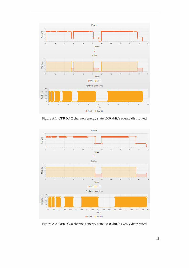
Figure A.1: OPB 3G, 2 channels energy state 1000 kbit/s evenly distributed
Figure A.2: OPB 3G, 8 channels energy state 1000 kbit/s evenly distributed
42

Figure A.3: OPB 3G, 2 channels energy state 1000 kbit/s burst mode
Figure A.4: OPB 3G, 8 channels energy state 1000 kbit/s burst mode
43

Figure A.5: Fast Broadcasting 3G, 2 channels energy state 1000 kbit/s evenly distributed
Figure A.6: Fast Broadcasting 3G, 8 channels energy state 1000 kbit/s evenly distributed
44

Figure A.7: Fast Broadcasting 3G, 2 channels energy state 1000 kbit/s burst mode
Figure A.8: Fast Broadcasting 3G, 8 channels energy state 1000 kbit/s burst mode
45
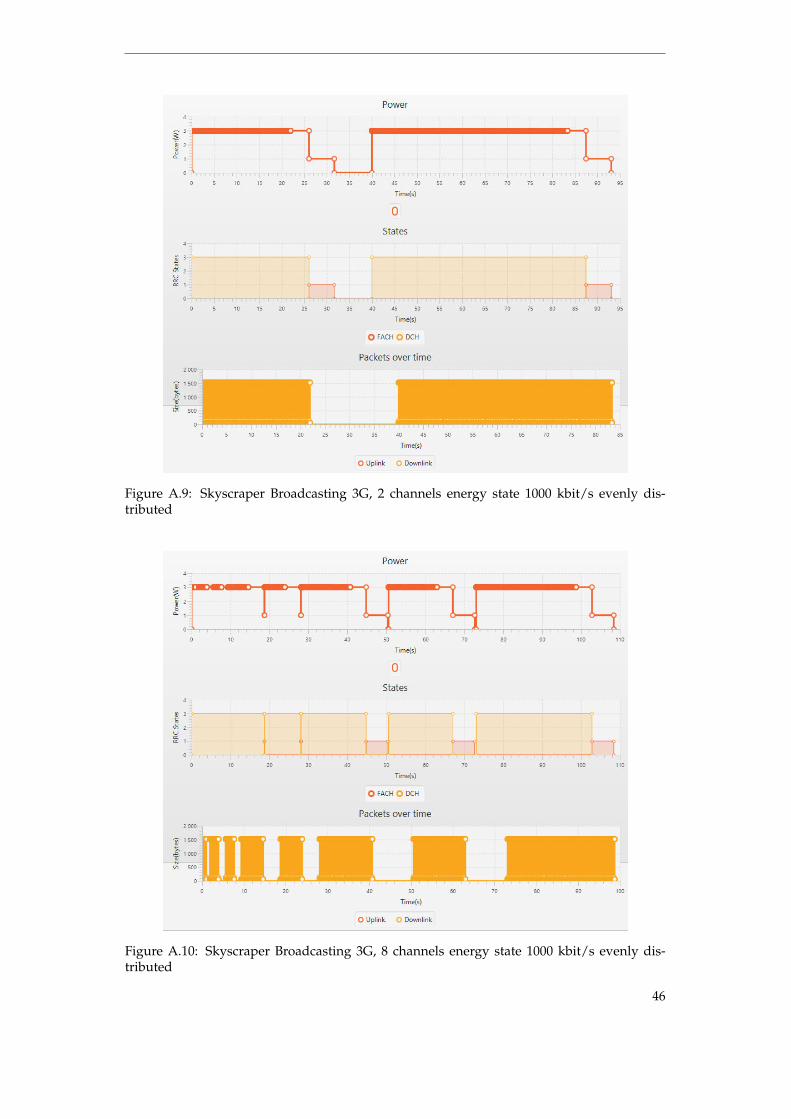
Figure A.9: Skyscraper Broadcasting 3G, 2 channels energy state 1000 kbit/s evenly dis-tributed
Figure A.10: Skyscraper Broadcasting 3G, 8 channels energy state 1000 kbit/s evenly dis-tributed
46

Figure A.11: Skyscraper Broadcasting 3G, 2 channels energy state 1000 kbit/s burst mode
Figure A.12: Skyscraper Broadcasting 3G, 8 channels energy state 1000 kbit/s burst mode
47

Figure A.13: Pyramid Broadcasting 3G, 2 channels energy state 1000 kbit/s evenly distributed
Figure A.14: Pyramid Broadcasting 3G, 8 channels energy state 1000 kbit/s evenly distributed
48

Figure A.15: Pyramid Broadcasting 3G, 2 channels energy state 1000 kbit/s burst mode
Figure A.16: Pyramid Broadcasting 3G, 8 channels energy state 1000 kbit/s burst mode
49
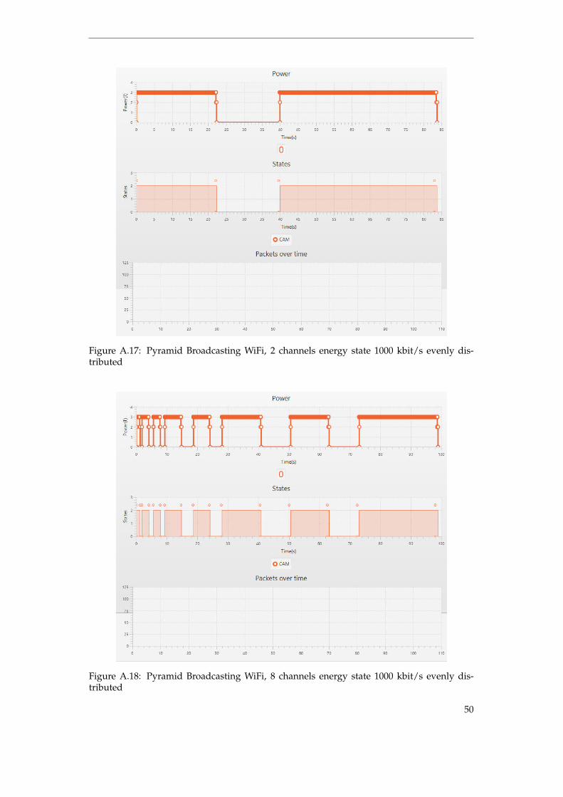
Figure A.17: Pyramid Broadcasting WiFi, 2 channels energy state 1000 kbit/s evenly dis-tributed
Figure A.18: Pyramid Broadcasting WiFi, 8 channels energy state 1000 kbit/s evenly dis-tributed
50

Linköping University Electronic Press
Upphovsrätt
Detta dokument hålls tillgängligt på Internet – eller dess framtida ersättare – från publiceringsdatum under förutsättning att inga extraordinära omständigheter uppstår.
Tillgång till dokumentet innebär tillstånd för var och en att läsa, ladda ner, skriva ut enstaka kopior för enskilt bruk och att använda det oförändrat för icke-kommersiell forskning och för undervisning. Överföring av upphovsrätten vid en senare tidpunkt kan inte upphäva detta tillstånd. All annan användning av dokumentet kräver upphovsmannens medgivande. För att garantera äktheten, säkerheten och tillgängligheten finns lösningar av teknisk och administrativ art.
Upphovsmannens ideella rätt innefattar rätt att bli nämnd som upphovsman i den omfattning som god sed kräver vid användning av dokumentet på ovan be-skrivna sätt samt skydd mot att dokumentet ändras eller presenteras i sådan form eller i sådant sammanhang som är kränkande för upphovsmannens litterära eller konstnärliga anseende eller egenart.
För ytterligare information om Linköping University Electronic Press se för-lagets hemsida http://www.ep.liu.se/.
Copyright
The publishers will keep this document online on the Internet – or its possible replacement – from the date of publication barring exceptional circumstances.
The online availability of the document implies permanent permission for anyone to read, to download, or to print out single copies for his/her own use and to use it unchanged for non-commercial research and educational purpose. Subsequent transfers of copyright cannot revoke this permission. All other uses of the document are conditional upon the consent of the copyright owner. The publisher has taken technical and administrative measures to assure authenticity, security and accessibility.
According to intellectual property law the author has the right to be mentioned when his/her work is accessed as described above and to be protected against infringement.
For additional information about the Linköping University Electronic Press and its procedures for publication and for assurance of document integrity, please refer to its www home page: http://www.ep.liu.se/.
© Christoffer Johansson, Martin Sjödin Jonsson