Embed Size (px)
Citation preview

Simulations of dispersed multiphase
flow at the particle level
Chemical Engineering
Delft University of Technology
Netherlands
[email protected]://homepage.tudelft.nl/s0j2f/
Jos Derksen

Multiphase flow
sediment transport
blood
predictive modeling & simulation
• flow dynamics• mass transfer & mixing• interface dynamics
@ the particle scale (“meso-scale”)(Pickering) emulsion
bubbly flow
collective behavior ↔ particle-scale processes

Macroscopic multiphase transportturbulent flow
“inertial” particles
wide spectrum of (length) scalesparticle size, tank size, turbulence scales
ν= ≈
25Re 10
ND ≈ 610pn
∼ 30 cm
Ayranci et al CES 2012

Unresolved vs resolved particles
particle size > grid spacingno need for empiricism*up to 104 particles
= > ∆2 pa d
∆
particle size < fluid grid spacingparticle dynamics based on empirical force correlationsup to 108 particles
*fine print
= < ∆2 pa d
“multi-scale”

Quick overview of numerics*
Lattice-Boltzmann method for solving the flow of interstitial fluid
3D, time-dependent
Explicitly resolve the solid-liquid interface: immersed boundary method
particle size typically 12 grid-spacings
Solve equations of linear and rotational motion for each sphere
forces & torques: directly (and fully) coupled to hydrodynamicsplus gravity
hard-sphere collisionsor soft interactions (mostly for non-spherical particles)
> ∆pd
fluid flow
particle motion
scalar
*Derksen & Sundaresan, JFM 587 (2007)
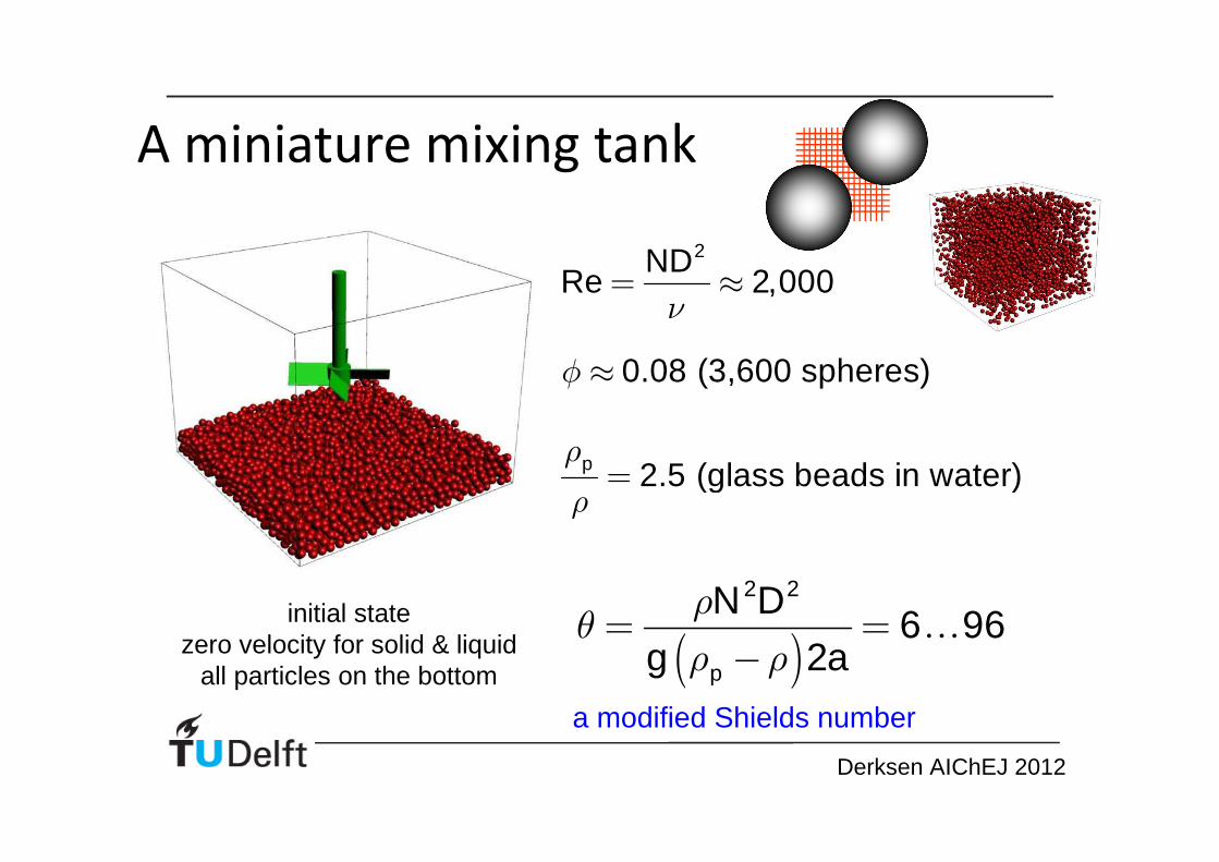
A miniature mixing tank
2
Re 2,000NDν
= ≈
( )
2 2
6 962p
N D
g a
ρθ
ρ ρ= =
−…
initial statezero velocity for solid & liquid
all particles on the bottom
0.08 (3,600 spheres)φ ≈
2.5 (glass beads in water)pρ
ρ=
a modified Shields number
Derksen AIChEJ 2012

Start-up of suspension process
0.08φ ≈
0.24φ ≈ tipu v0 1
0.24φ ≈

Experimental validation@ Institut de Mécanique des Fluides de Toulouse
refractive index matching for optical access
@ Beijing University of Chemical Technology†
a liquid fluidization experiment*..
..& our simulation**
*Duru, Guazelli JFM 2002**Derksen, Sundaresan JFM 2007
†Mo et al AIChEJ 2015

More experimental validation
starting from a vertical orientation
Becker Can. J. Chem. Eng 1959
very simple experimentsRe
u Dν
∞∞ =
a High School experiment

Mass transfer• start with zero concentration in the liquid• apply a c=1 boundary condition at the
particle surface• solve a convection-diffusion equation in c
vertical cross section
horizontal cross section
Liquid systems: resolution is a seriousconcern given high Schmidt numbers
hydrodynamic resolution2a=dp=16∆
( )3Sc 10Oν
≡ =Γ

Coupled overlapping domains*spherical grid attached to particle
Cartesian outer grid
Communication between the grids:linear interpolation• velocity on the spherical grid is imposed from the outer grid• concentration fields are two-way coupled between the grids
sphere & spherical grid move relative to Cartesian grid
* Derksen AIChEJ 2014** Derksen CEJ 2014
multiple particles will have overlapping
shells**
...mixing rules…

Two-sphere benchmarkoverall flow in x-direction

Fixed beds versus moving spheres
ν
φ
= =
=
= 3
2Re 1
0.2
Sc 10
u a
ν
φ
ρ ρ
−= =
=
=
=ℓ
3
2Re 1
0.2
Sc 10
4
p
p
u v a
sedimenting spheres g

Compare Sherwood numbers
4pρ ρ =ℓ
the role of the density ratio
fixed bed level
fixed bed level
Re 1
0.2φ
=
=

Some more mass transfer
hot melt extrusion* breakthrough in a micro reactor**
most of the yellow agent adsorbs on the particles
*Derksen et al ChERD 2015**Derksen Micro Nano Fluidics 2014
“industrial” applications

Liquid-liquid dispersions (emulsions)
flow dynamics ↔ drop size distribution ↔ interfacial area ↔inter-phase mass transfer ↔ apparent rheology ↔ stability ↔
product formulation
break-up
Basic events
coalescence
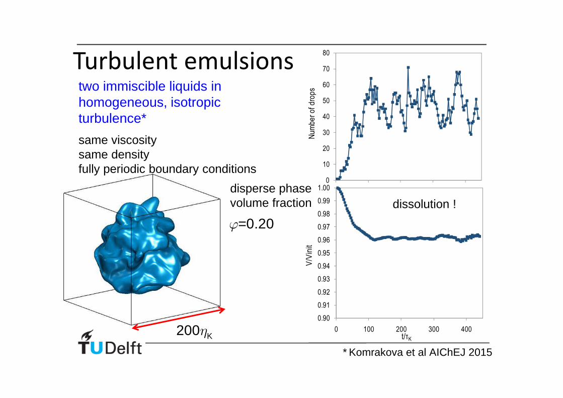
Turbulent emulsions
0
10
20
30
40
50
60
70
80
0 100 200 300 400
Nu
mb
er
of
dro
ps
t/τK
0.90
0.91
0.92
0.93
0.94
0.95
0.96
0.97
0.98
0.99
1.00
0 100 200 300 400
V/V
init
t/τK
=0.20ϕ
dissolution !
200 Kη
disperse phase volume fraction
two immiscible liquids in homogeneous, isotropic turbulence*
same viscositysame densityfully periodic boundary conditions
* Komrakova et al AIChEJ 2015

A methods slide: binary liquids
coupled with hydrodynamics through body force � = −���
chemical potential
� =��
��= � � − 1 − ���
�
�+ �∙ �� = ���
advection-diffusion
Briant, Yeomans Phys Rev E 2004
-2 -1 0 1 2�
�: order parameter controls composition�
� = 2�
� =
2 2
3�
interface thickness surface tension�
-1
0
1
-4 -2 0 2 4
�/�
a “diffuse” interface
proper interface is resolution: �≈1 − 2

Make the flow simpler: breakup in shear
ReCa= 00.4 12 .06 λ= =
just above Cac (Ca-critical)
resolution: a=20
a=25
a=30
quick dissolution
The good news:breakage / non-breakage is largely independent of
resolution
Ca maµ γ
σ=
ɺ
Komrakova et al IJMF 2014
Capillary number
starting point: spherical drop with radius a

Coalescence in shear
Chen et al. Langmuir 2009
Theory, Experiments, and Motivation
approach
coalescence
film drainage
sliding
complex interfaces:
charge, steric effects, variable tension
++++++
++
++++
++++
++
++
++
++
++
++++
++++++
simulations at critical conditions are challenging• topological change; 30 nm film vs. 100 µm drops
clean polymer systems• hydrodynamics, surface tension, van der Waals forces
charged surfaces and electrolytes• additional electrostatic interactions

Uncharged drops
Ca = 0.095
Ca = 0.080
capillary number determines outcome of collision
sliding
coalescence
Shardt, Derksen, Mitra Langmuir 2013
CaRρν γσ
=ɺ
Guido, Simeone J Fluid Mech (1998)
� = 2�
� = �
�
��
�
Δ
Δ!
" #$ =2�%
�
�%
�%
Δ /2" = &. ()
Ca = 0.085temporary bridge
uniform density & viscosity

We are (fairly) grid independent
Ca = 0.08
Ca = 0.09
Ca = 0.1
Doubling interface resolution does not change outcome. ∴ adequately resolved with � = 2
Solid black: " = 75, � = 4 Dashed red: " = 37.5, � = 2

CaRρν γσ
=ɺ
Critical capillary numbers
….towards lower Δ /2" to compare with experiments
RΔY

Ca = 0.1
…need higher resolution
Δ /2" = 0.2
Ca = 0.25
Ca = 0.2
De Bruyn et al. JCIS 2013
" = 200/0��123�41�5
Shardt, Mitra, Derksen Langmuir 2014
CaRρν γσ
=ɺ

0 2 4 6 8 10 12
0
5
10
15
20
Time,
Fil
m t
hic
kn
ess
(l.
u.)
Ca = 0.05
Ca = 0.10
Ca = 0.01
Ca = 0.20
Ca = 0.25
Ca = 0.30
Evolution of film thickness
#$�
Ca = 0.01Ca = 0.05
Ca = 0.1
Ca = 0.2
Ca = 0.25, 0.3
Critical film thickness
critical capillary number 0.1 to 0.25 at 67
8= 0.2
a good question would be: how big are these drops actually?an estimate can be based on minimum film thicknessminimum film thickness 5 – 10 l.u. ~ 30 nm
⇒ " = 200: 0.6 − 1.2�;
imagine simulating coalescence of 1 mm
drops

Charged drops
Ca 0.06aρν γσ
= =ɺ
1 0.2aκ− =
uncharged
charged with Debye length
increasing electric field strength
factor 10 each time
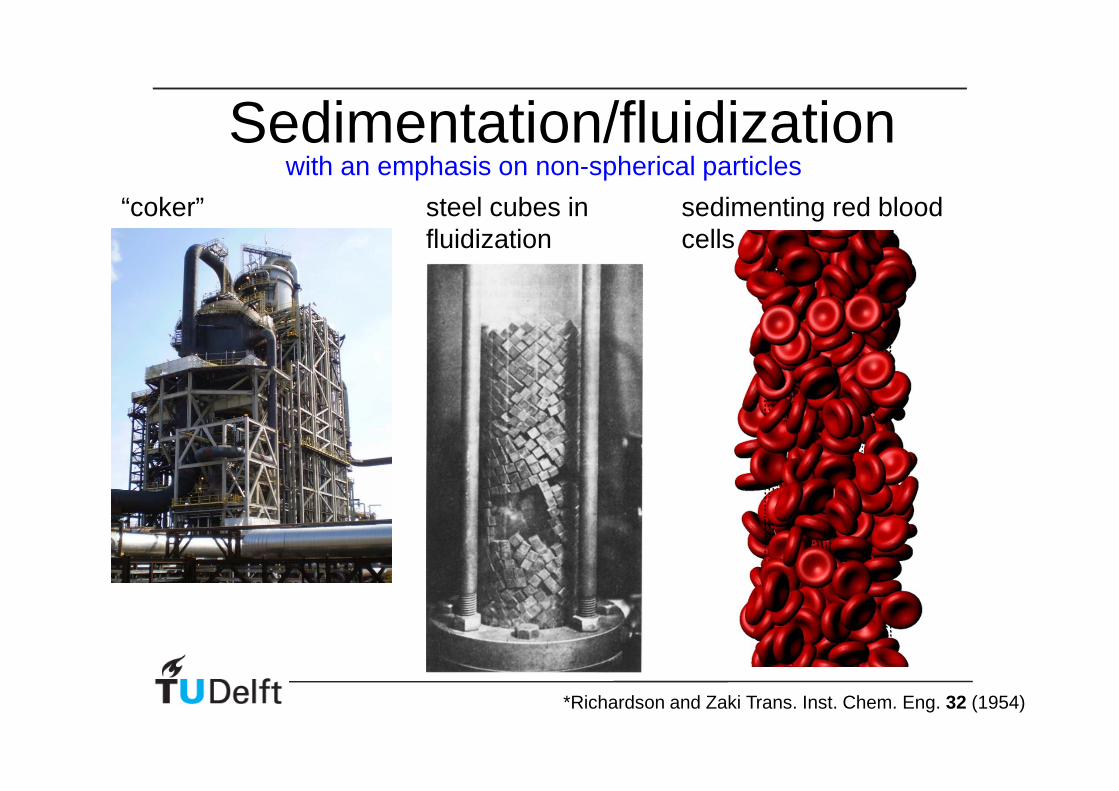
Sedimentation/fluidization“coker”
*Richardson and Zaki Trans. Inst. Chem. Eng. 32 (1954)
steel cubes in fluidization apparatus*
sedimenting red blood cells
with an emphasis on non-spherical particles

RBC’s as sample non-spherical particles
( )F k xδ= − ∆
x∆
* Shardt & Derksen, IJ Multiphase Flow 47 (2012)
Specific challenges*
• collision handlingrepulsive spring force between surface points also used for immersed boundary
• low density ratiouse modified finite difference method for stability
• high solids volume fraction (~0.45)• compaction procedure for initialization• frequent collisions
1.07pρ ρ =

Settling of a dense suspension
291 particles� = 0.35
removingparticles reveals flow cross-section
all boundariesare periodic
resolutionD = 20 nodes
body force on fluid
balances gravity

Hindered settling
1 − �
void fraction
Re =�>?@ABC
D
Richardson-Zaki (RZ)
Re 18.2∞ =The RZ fit suggests
→ an - on average - inclined RBC
( )1nslipu
uφ
∞
= −

Typical human ESR is 3 – 9 mm/h
Simulations: 0.18 mm/h
surface forces between RBCs and proteins in blood cause agglomeration
Human erythrocyte sedimentation rateU. Woermannedu.cpln.ch/hemosurf/data/Lab-Images/all_ESRs.jpg
ESR blood tests
@ � = 0.35

AcknowledgementsSponsorsCollaborators & students
Gaopan Kong & Eric Climent in Toulouse
Junyan Mo, Zhipeng Li & Bruce Gao in Beijing
Alexandra Komrakova, Inci Ayranci, Suzanne Kresta, Orest Shardt & Jue Wang in Edmonton
Sankaran Sundaresan in Princeton

Beyond continuum modelingexample: aggregation of nanoparticles&liquid bridges
Molecular Dynamics
8 nm spheres in a classical Lennard-Jones fluid
(red=vapor; yellow=liquid; green=solid)
22
1
1R
f RR
σπ = −
(+ is attractive)
TiO2nanoparticles
1 3
NB: 3nmmolar
Av
VN
≈
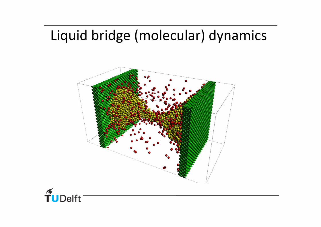
Liquid bridge (molecular) dynamics