Simulation Optimization of Manufacturing Takt Time for a

Simulation Optimization of Manufacturing Takt Time for a Leagile Supply Chain with a De-coupling Point

1. Introduction

Supply chains often pose challenges in decision making as it involves several entities and parameters like vendors, warehouses, logistics supports, variable demands and costs, etc. Uncertainties in events and forecasted demands add more complexities to this problem. In recent times, the demand for products is highly unpredictable owing to the market dynam-ics and uncertainties. Further, the need of providing a wide range of product variety to cater the custom-ized demands also aggravate the problem. In a global manufacturing environment, more and more prod-ucts with shorter life cycles have been introduced to

the market. In order to retain the core competence of manufacturing enterprise, its systems and supply chains should be altered in response to the changing requirement [1]. In the present dynamic world, in or-der to be competitive, it is integral that the customer demand be met unceasingly. The market demand is volatile because of lot of factors such as increasing demands for customization, advances in technology, seasonal variations, catastrophes, etc. It is, therefore, imperative that advancements in modeling of supply chain management systems rise up to meet the chal-lenges [2-4].

In this context, the concepts of lean and agile sup-ply chain models are worth a mention. Supply chain

Achieving agility with leanness in supply chains is considered to be a challenge for industry and academia. In order to cope with dynamic demands at extreme downstream, buffer stocks at various points on the supply chain can be seen as a solution. Although it may improve the agility feature but extra inventories at warehouses affects the leanness of the supply chain adversely. The aim of the present paper is to address this issue by finding an optimum rate of production at the factory which is directly related to Takt time concept of lean manu-facturing in order to fulfill the dynamic demand patterns at the downstream retailers end while minimizing intermediate stock inventories. The model is conceived as a leagile supply chain with a de-coupling point at the warehouse or distribution center between retailers and plant. A discrete event simulation model for the supply chain is developed in WITNESS® to experiment with various rates of production before finding the optimum value. The two performance measures representing fulfillment of product demands and inventory carrying costs are expressed in equivalent cost units for optimization. Two demand scenarios for a two product supply chain are simulated to identify the optimal rate of production while illustrating the solution methodology. The simulation optimization approach to address this problem of leagile supply chain is found to be effective and practical.

Article history:

Received October 24, 2020 Revised April 1, 2021Accepted April 5, 2021Published online May 13, 2021

Keywords:Simulation Optimization; WITNESS®; Lean Manufacturing; Leagile Supply Chain; Takt Time; Decoupling point

*Corresponding author:Laxmi Narayan [email protected]

ISSN 2683-345X

DOI: http://doi.org/10.24867/IJIEM-2021-2-280Published by the University of Novi Sad, Faculty of Technical Sciences, Novi Sad, Serbia. This is an open access article distributed under the CC BY-NC-ND 4.0 terms and conditions

A B S T R A C T A R T I C L E I N F O

International Journal of Industrial Engineering and Management

Volume 12 / No 2 / June 2021 / 102 - 114

Original research article

journal homepage: http://ijiemjournal.uns.ac.rs/

L. N. PattanaikDepartment of Production Engineering, Birla Institute of Technology, Mesra, Ranchi, India

103Pattanaik

International Journal of Industrial Engineering and Management Vol 12 No 2 (2021)

agility is a key to adapting to market variations more efficiently, inventory reduction, enabling firms to re-spond to demand more quickly and integrating with suppliers more effectively.

Lean supply chains were primarily designed for the removal of waste from all the related func-tions. Leanness means developing a value stream to eliminate all waste and to achieve a balanced pro-duction schedule. However, lean supply chains are considered to be attainable for relatively stable and predictable demand with low variety. On the other hand, agile supply chains provide with the solutions to problems where there is fluctuating demand with high variety. These two paradigms of lean and agile supply chains are merged to develop the conceptual model of leagile supply chain. The tradeoff between leanness and agility was balanced in a leagile supply chain system by identifying an appropriate de-cou-pling point [5].

De-coupling point is defined as the point where the model changes from push to pull based system. The push model works on the principle of anticipa-tion of customer orders while pull model is executed when customer demand is known with certainty. The supply chain exhibit lean features before the decou-pling point from the upstream and agility after it to-wards downstream. The de-coupling point is located such that it favors the need for responding to a fluc-tuating demand in downstream while allowing a stat-ic level of manufacturing schedule in the upstream. The decoupling point can be considered as the point where order-driven and the forecast driven functions merge [5-6].

One of the key characteristic of the lean model presented in this paper is the takt. It is a preset pro-duction rhythm associated with lean philosophy and defined as the time interval between two consecutive finished products to ensure the continual flow of fin-ished products needed to meet customer demand. The reciprocal of production rate is mathematically equivalent to the takt time. The benefits of adopting takt during production include balanced utilization of resources, minimization of waste in finished invento-ry, fulfillment of demand in schedule, etc.

The aim of the present work is to find the opti-mum production rate or takt time of a manufactur-ing/assembly system associated with a leagile supply chain having stochastic and dynamic demands at multiple retailers. The objectives are to avoid excess stocks of inventory at warehouse (considered as the de-coupling point) while meeting the demands of the downstream retailers. A discrete-event simulation model is developed for the leagile supply chain to

experiment with varying production rates under dy-namic demand scenarios.

In section 2, literature pertaining to leagile supply chains and simulation based optimization of supply chains are compiled. The leagile supply chain mod-el along with various assumptions, parameters and constraints, objectives for optimization are described in section 3. In section 4, experimentation with the model developed in WITNESS® is illustrated using hypothetical data sets for two stochastic demand pe-riods, various costs, capacity of warehouse and pro-duction rates. The output from simulation model is analyzed to arrive at optimal takt or production rate for two different product types in each demand sce-nario. The concluding remarks and future scope of the work are presented in the last section.

2. Literature review

This literature review encompassed the relevant areas for the present work like agile supply chains, leanness in supply chain, leagile supply chains, de-coupling point concept, application of simulation optimization and some case studies. Literature from these areas are presented here in the same order.

Over the years it has become apparent that mar-kets are now increasingly volatile and less predictable. So the need for a more agile response has grown. Agility is the company-wide capability that includes organizational structures, information systems, logis-tics, procurement and production to respond to vol-atility. In such market conditions of increasing levels of product variety and customization, the ability to re-spond to customer orders in time can provide a crit-ical competitive advantage. Xiaomei and co-authors [7] emphasized that the traditional supply chains fail to cope up with the uncertainty in the market owing to development of economy, information technology and shortened product life cycle. Preference of cus-tomized and diversified products by end customer, uncertainties and disruptions necessitates an inherent flexibility within the supply chain network to ensure the reconfigurability; a primary requirement when developing an agile supply chain system [8-11].

Lean manufacturing concepts have been in prac-tice over few decades and well accepted as an effec-tive tool. The roots of lean philosophy can be traced to Toyota Production Systems (TPS) of Japan. The lean approach is applicable where there is relatively stable and predictable demand with low variety [12]. Leanness and agility, even being very different as concepts have been successfully merged within total supply chains by [5]. The combination of agility and

104 Pattanaik


leanness into supply chain with the strategic place-ment of a de-coupling point is termed as leagility [13]. The drawback of lean supply chain is the inability to respond to end customer customized demands, thus, leagile supply chain has been proposed in the indus-try to combine the advantages of both agile and lean paradigms. Compared with traditional supply chains, leagile supply chain has the advantages of informa-tion sharing, shorten length of chain, order guidance and close cooperation among stake holders.

Christopher and Towil [14] put forward the idea to bring together the lean and agile philosophies to highlight the difference in the two approaches and suggested that these can be combined for better re-sults and advantages. The leagile supply chain focus is to effectively handle uncertain demands by deferring the products as far as possible towards the customer end. Hoek [15] highlighted benefits of the postpone-ment strategy, like reduced inventory, increase in flex-ibility and multiplicity of production, easy forecasting and better personalization according to the customer demand. The importance and advantages of leagile supply chain has been discussed by a number of re-searchers [9] [16-17]. Ambe and Badenhorst-Weiss [18] proposed a framework for leagile supply chain appropriate for the auto industry and the implemen-tation of which would result in cost reduction and the supply chain being more responsive. Shukla and Wan [19] in their work presented an optimization approach for a leagile inventory model. They first formulated a non-linear integer programming model which was solved in real-time using three variants of genetic algorithm. Komoto and other authors [20] in their paper on multi-objective reconfiguration meth-od of supply chains through discrete event simulation worked on a case study to show how the multi-objec-tive optimization has been implemented in discrete event simulation. Peirleitner et al. [21] compared two different solution methods for determining optimal parameter settings for lot size Q and reorder points. The first method is an analytical optimization mod-el assuming a single-stage, single-product inventory system which is applied independently for all supply chain partners. Optimal parameters are identified for all partners and then re-evaluated in the dynamic and stochastic simulation model. Results show that if analytical optimal parameters are evaluated with sim-ulation, which includes the dynamics and interdepen-dencies between the supply chain members, lower service levels than initially predefined were achieved. A synchronized logistic model to address various is-sues of a dynamic supply chain was developed [22].

Considering supply chain as a complex and dy-

namic system as compared to other analysis tools, simulation has an edge due to the dynamicity and randomness it can provide to the user. Simulation has been used for years in the areas of supply chain, manufacturing and business has led to a wide range of successful applications in different areas such as design, planning and control, strategy making, re-source allocation, training, etc. [23].

Simulation is the best practice to evaluate the sys-tem performance closely to real situation. Simulation Optimization (SO) appears as popular technique and has received considerable attention from both sim-ulation researchers and practitioners which can be achieved using software packages [24]. Ran et al. [25] presented a review on applications of SO to design and operation of manufacturing systems to address the inherent stochastic properties. By dividing the problems into local and global optimization category, they further classified on the basis of discrete or con-tinuous nature. Maedeh et al. [26] solved a multi-ob-jective problem using a hybrid of SO with regression analysis for unreliable and unbalanced production lines. In a recent review, classified applications of simulation optimization to supply chain problems in general with focus on resilience was found. Hybrid-ization of SO with meta-heuristics was suggested as a prospective future research direction [27].

Demand uncertainty, in particular is an important factor to be considered in the supply chain design and operations. Due to advance of global manufacturing, the decentralized optimization of multi-tier supply chains for multiple retailers and manufacturers be-comes more and more important. Nishi and Yoshida [28] have addressed the optimization of multi-period bi-level supply chains under demand uncertainty. The optimization algorithm to derive Stackelberg equilib-rium for multi-period bi-level supply chain planning problem is developed and dealt using simulation. Matheus et al. [29] proposed a simulation based op-timization approach to cope with supply chain plan-ning and control of high uncertainty scenarios i.e. stochastic behavior and dynamic events, addressing areas of material inventory, production and trans-portation. In their work, they discussed a simulation based optimization approach to simultaneously deal with the planning and control of the material inven-tory, production and transportation areas combining the capabilities from metaheuristics and simulation models. Their proposed approach was implemented in a test case and claimed a convergence to a solu-tion within a short span of time. Liotta et al. [30] also opine that simulation-based optimization is a strategy for dealing with uncertainty in the supply chain. In

105Pattanaik


addition, Truong and Azadivar [31] suggested that managing a supply chain is much more complex than dealing with one facility because of existing conflict-ing objectives and dynamic properties of the system. Hence, they proposed a simulation-based approach to deal with supply chain configuration design.

A case study of a mobile phone manufactur-ing industry was undertaken. They studied mobile phone firm’s operational configuration and pro-posed real-time decision support mechanism based on agent-based discrete-event simulation to estimate performance of average inventory levels over the system-wide supply chain [1]. Using WITNESS®, a supply chain model can be built and analyzed with-out the need to physically carry out tests in real life [32].

In this paper, a leagile supply chain model is sim-ulated using WITNESS® to give optimum takt times for different demand periods with conflicting objec-tives of minimizing stock-outs and inventory costs.

3. Model of the leagile supply chain

The supply chain adopted in the present paper has leagile characteristics to meet volatile market de-mand as well as to ensure optimum inventory level to minimize cost. To achieve this, the decoupling point is set at the warehouse which is between the production facility and the retailer(s). Products are continuously manufactured at a predetermined rate based on takt time and pushed to the warehouse after which the goods are pulled by the retailer(s) accord-ing to the customer demand. Leanness is achieved by producing the optimum amount and avoiding ex-cess inventory and cost associated with it while agility

is achieved by satisfying the customers by adjusting the takt time and reorder points according to the de-mands.

Takt is a pre-determined production rhythm asso-ciated with lean philosophy and defined as the time interval between two consecutive finished products needed to meet customer demand. It is expressed as the ratio between total available time for production and total customer demands during that duration. The reciprocal of production rate is mathematically equivalent to the takt time. By adopting takt during production, balanced utilization of resources, mini-mization of waste in finished inventory, fulfillment of demand in schedule, etc. can be achieved.

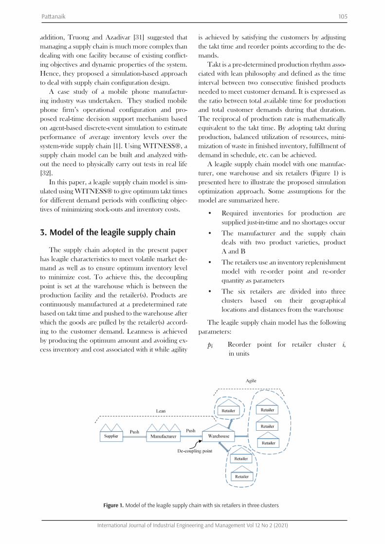
A leagile supply chain model with one manufac-turer, one warehouse and six retailers (Figure 1) is presented here to illustrate the proposed simulation optimization approach. Some assumptions for the model are summarized here.

• Required inventories for production are supplied just-in-time and no shortages occur

• The manufacturer and the supply chain deals with two product varieties, product A and B

• The retailers use an inventory replenishment model with re-order point and re-order quantity as parameters

• The six retailers are divided into three clusters based on their geographical locations and distances from the warehouse

The leagile supply chain model has the following parameters:

pi Reorder point for retailer cluster i, in units

Figure 1. Model of the leagile supply chain with six retailers in three clusters

106 Pattanaik


q Reorder quantity, in units

Ri Retailer cluster i

DA Demand for product type A, units/day

DB Demand for product type B, units/day

MPA Market price of product A per unit

MPB Market price of product B per unit

CPA Cost price of product A per unit

CPB Cost price of product B per unit

ti Minimum transportation time from warehouse to retailer cluster i, days

αi Exponential variation in transportation time from warehouse to retailer cluster i, days

Ti Transportation times from warehouse to retailer cluster i, Ti = (ti + αi), days

ηA The optimum production rate of product type A at the plant, units/day

ηB The optimum production rate of product type B at the plant, units/day

λA Production capacity of the plant for product A, units/day

λB Production capacity of the plant for product B, units/day

Rc Retailer holding capacity, units

Wc Warehouse storage capacity, units

ɣi Delivery capacity from warehouse to retailer cluster i, units

TL Total loss incurred for a product, cost unitsTI Total loss due to excess inventory at

warehouse for a product, cost unitsTS Total loss due to unavailability of a product

at retailers, cost unitsIW Inventory at warehouseIT Threshold level for inventory

The above described model is simulated to find the optimum production rate for two product types with the objective to maximize the service level (availability of products at retailers) and at the same time minimize the inventory level at the warehouse. A higher inventory level improves the service level means the customer demands are fulfilled with less stock-out situations but higher inventory can be costly for the firm as excess inventory will result in greater storage costs, risk of obsolescence, pilferage, insur-ance premium, etc. On the other hand lower inven-tory level can results in stock-outs which will impair the service levels causing loss of sales and goodwill of

the customer.In this paper a supply chain model is optimized

having two conflicting objectives to maximize the ser-vice level and minimize the inventory level.

The two objectives were combined to calculate the total loss incurred due to high inventory at the warehouse and losses due to poor service level at re-tailers. Losses due to high inventory are considered only after the inventory level at the warehouse cross-es a threshold level IT.

The takt based production rate with the lowest value of total loss TL gives the optimum production rate for the respective demand cycle

4. Simulation optimization using WITNESS®

Simulation optimization is considered as an effec-tive analytical tool to arrive at the optimal solution without implementing any classical, conventional or meta-heuristic based computation. Problems in sup-ply chains are predominantly of combinatorial opti-mization types, which can be solved using simulation optimization with lesser computational complexity.

The software used in the present work, WIT-NESS® is industry-standard simulation software with the ability to model a wide range of process and op-eration tasks. It is a software platform for dynamic system modeling and simulation, which is developed by the British Lanner, to cater the needs of industrial and business systems and processes (Men and Zhou, 2011). It has a wide range of application areas, a large number of model elements, a powerful simulation engine, a convenient graphical interface operation function and a hierarchical modeling function.

The leagile supply chain model is optimized using the approach of simulation optimization. Simulation optimization deals with the situation in which the ana-lyst would like to find which of the many sets of mod-el specifications (input parameters and/or structural

107Pattanaik


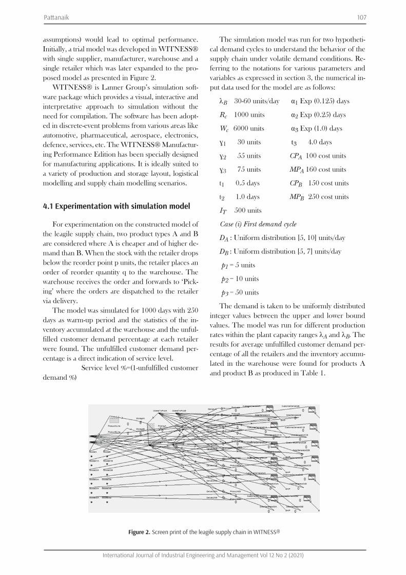
assumptions) would lead to optimal performance. Initially, a trial model was developed in WITNESS® with single supplier, manufacturer, warehouse and a single retailer which was later expanded to the pro-posed model as presented in Figure 2.

WITNESS® is Lanner Group’s simulation soft-ware package which provides a visual, interactive and interpretative approach to simulation without the need for compilation. The software has been adopt-ed in discrete-event problems from various areas like automotive, pharmaceutical, aerospace, electronics, defence, services, etc. The WITNESS® Manufactur-ing Performance Edition has been specially designed for manufacturing applications. It is ideally suited to a variety of production and storage layout, logistical modelling and supply chain modelling scenarios.

4.1 Experimentation with simulation model

For experimentation on the constructed model of the leagile supply chain, two product types A and B are considered where A is cheaper and of higher de-mand than B. When the stock with the retailer drops below the reorder point p units, the retailer places an order of reorder quantity q to the warehouse. The warehouse receives the order and forwards to ‘Pick-ing’ where the orders are dispatched to the retailer via delivery.

The model was simulated for 1000 days with 250 days as warm-up period and the statistics of the in-ventory accumulated at the warehouse and the unful-filled customer demand percentage at each retailer were found. The unfulfilled customer demand per-centage is a direct indication of service level.

Service level %=(1-unfulfilled customer demand %)

The simulation model was run for two hypotheti-cal demand cycles to understand the behavior of the supply chain under volatile demand conditions. Re-ferring to the notations for various parameters and variables as expressed in section 3, the numerical in-put data used for the model are as follows:

λB 30-60 units/day α1 Exp (0.125) days

Rc 1000 units α2 Exp (0.25) days

Wc 6000 units α3 Exp (1.0) days

ɣ1 30 units t3 4.0 days

ɣ2 55 units CPA 100 cost units

ɣ3 75 units MPA 160 cost units

t1 0.5 days CPB 150 cost units

t2 1.0 days MPB 250 cost units

IT 500 units

Case (i) First demand cycle

DA : Uniform distribution [5, 10] units/day

DB : Uniform distribution [5, 7] units/day

p1 = 5 units

p2 = 10 units

p3 = 50 units

The demand is taken to be uniformly distributed integer values between the upper and lower bound values. The model was run for different production rates within the plant capacity ranges λA and λB. The results for average unfulfilled customer demand per-centage of all the retailers and the inventory accumu-lated in the warehouse were found for products A and product B as produced in Table 1.

Figure 2. Screen print of the leagile supply chain in WITNESS®

108 Pattanaik


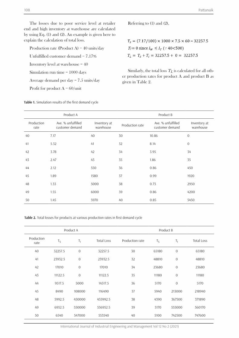
The losses due to poor service level at retailer end and high inventory at warehouse are calculated by using Eq. (1) and (2). An example is given here to explain the calculation of total loss.

Production rate (Product A) = 40 units/day

Unfulfilled customer demand = 7.17%

Inventory level at warehouse = 40

Simulation run time = 1000 days

Average demand per day = 7.5 units/day

Profit for product A = 60/unit

Referring to (1) and (2),

Similarly, the total loss TL is calculated for all oth-er production rates for product A and product B as given in Table 2.

Table 1. Simulation results of the first demand cycle

Table 2. Total losses for products at various production rates in first demand cycle

Product A Product B

Production rate

Ave. % unfulfilled customer demand

Inventory at warehouse Production rate Ave. % unfulfilled

customer demand Inventory at warehouse

40 7.17 40 30 10.86 0

41 5.32 41 32 8.14 0

42 3.78 42 34 3.95 34

43 2.47 43 35 1.86 35

44 2.12 550 36 0.86 450

45 1.89 1580 37 0.99 1920

48 1.33 5000 38 0.73 2950

49 1.55 6000 39 0.86 4200

50 1.45 5970 40 0.85 5450

Product A Product B

Production rate TS TI Total Loss Production rate TS TI Total Loss

40 32257.5 0 32257.5 30 65180 0 65180

41 23932.5 0 23932.5 32 48810 0 48810

42 17010 0 17010 34 23680 0 23680

43 11122.5 0 11122.5 35 11180 0 11180

44 9517.5 5000 14517.5 36 5170 0 5170

45 8490 108000 116490 37 5940 213000 218940

48 5992.5 450000 455992.5 38 4390 367500 371890

49 6952.5 550000 556952.5 39 5170 555000 560170

50 6540 547000 553540 40 5100 742500 747600

109Pattanaik


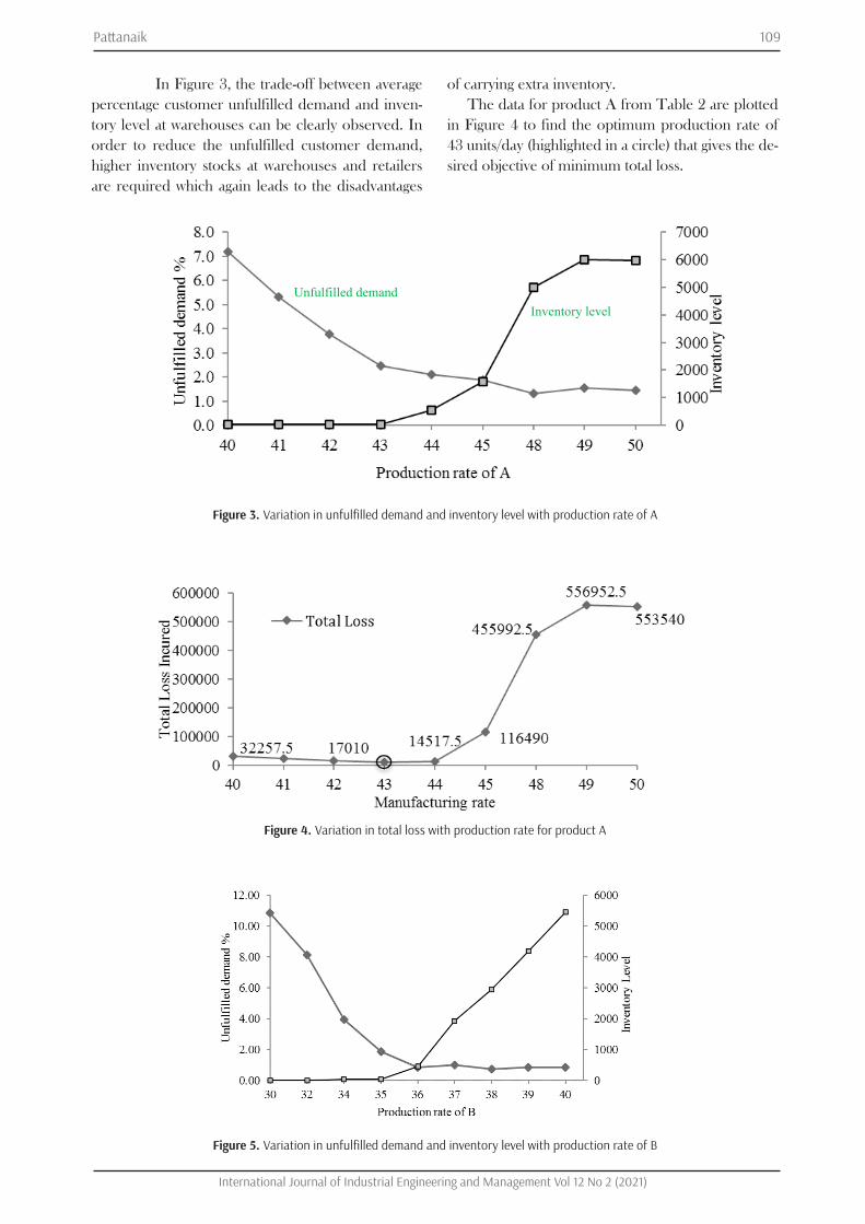
In Figure 3, the trade-off between average percentage customer unfulfilled demand and inven-tory level at warehouses can be clearly observed. In order to reduce the unfulfilled customer demand, higher inventory stocks at warehouses and retailers are required which again leads to the disadvantages

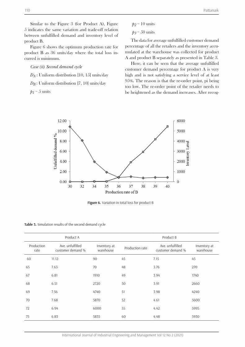
of carrying extra inventory. The data for product A from Table 2 are plotted

in Figure 4 to find the optimum production rate of 43 units/day (highlighted in a circle) that gives the de-sired objective of minimum total loss.

Figure 3. Variation in unfulfilled demand and inventory level with production rate of A

Figure 4. Variation in total loss with production rate for product A

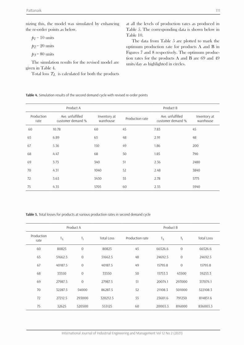
Figure 5. Variation in unfulfilled demand and inventory level with production rate of B

Unfulfilled demand Inventory level

110 Pattanaik


Figure 6. Variation in total loss for product B

Similar to the Figure 3 (for Product A), Figure 5 indicates the same variation and trade-off relation between unfulfilled demand and inventory level of product B.

Figure 6 shows the optimum production rate for product B as 36 units/day where the total loss in-curred is minimum.

Case (ii) Second demand cycle

DA : Uniform distribution [10, 15] units/day

DB : Uniform distribution [7, 10] units/day

p1 = 5 units

p2 = 10 units

p3 = 50 units

The data for average unfulfilled customer demand percentage of all the retailers and the inventory accu-mulated at the warehouse was collected for product A and product B separately as presented in Table 3.

Here, it can be seen that the average unfulfilled customer demand percentage for product A is very high and is not satisfying a service level of at least 95%. The reason is that the re-order point, pi being too low. The re-order point of the retailer needs to be heightened as the demand increases. After recog-

Table 3. Simulation results of the second demand cycle

Product A Product B

Production rate

Ave. unfulfilled customer demand %

Inventory at warehouse Production rate Ave. unfulfilled

customer demand % Inventory at warehouse

60 11.12 90 45 7.15 45

65 7.63 70 48 3.76 270

67 6.81 1910 49 3.94 1740

68 6.51 2720 50 3.91 2660

69 7.56 4740 51 3.98 4240

70 7.68 5870 52 4.61 5600

72 6.94 6000 55 4.42 5995

75 6.83 5835 60 4.48 5930

111Pattanaik


nizing this, the model was simulated by enhancing the re-order points as below.

p1 = 10 units

p2 = 20 units

p3 = 80 units

The simulation results for the revised model are given in Table 4.

Total loss TL is calculated for both the products

at all the levels of production rates as produced in Table 5. The corresponding data is shown below in Table 10.

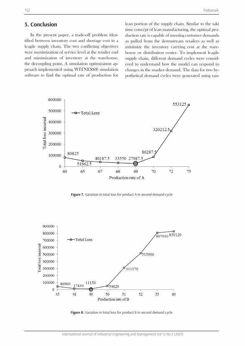
The data from Table 5 are plotted to mark the optimum production rate for products A and B in Figures 7 and 8 respectively. The optimum produc-tion rates for the products A and B are 69 and 49 units/day as highlighted in circles.

Table 4. Simulation results of the second demand cycle with revised re-order points

Table 5. Total losses for products at various production rates in second demand cycle

Product A Product B

Production rate

Ave. unfulfilled customer demand %

Inventory at warehouse Production rate Ave. unfulfilled

customer demand % Inventory at warehouse

60 10.78 60 45 7.83 45

65 6.89 65 48 2.91 48

67 5.36 150 49 1.86 200

68 4.47 68 50 1.85 790

69 3.73 340 51 2.36 2480

70 4.31 1040 52 2.48 3840

72 3.63 3430 55 2.78 5775

75 4.35 5705 60 2.35 5940

Product A Product B

Production rate TS TI Total Loss Production rate TS TI Total Loss

60 80825 0 80825 45 66526.6 0 66526.6

65 51662.5 0 51662.5 48 24692.5 0 24692.5

67 40187.5 0 40187.5 49 15795.8 0 15795.8

68 33550 0 33550 50 15753.3 43500 59253.3

69 27987.5 0 27987.5 51 20074.1 297000 317074.1

70 32287.5 54000 86287.5 52 21108.3 501000 522108.3

72 27212.5 293000 320212.5 55 23601.6 791250 814851.6

75 32625 520500 553125 60 20003.3 816000 836003.3

112 Pattanaik


5. Conclusion

In the present paper, a trade-off problem iden-tified between inventory cost and shortage cost in a leagile supply chain. The two conflicting objectives were maximization of service level at the retailer end and minimization of inventory at the warehouse, the decoupling point. A simulation optimization ap-proach implemented using WITNESS® simulation software to find the optimal rate of production for

lean portion of the supply chain. Similar to the takt time concept of lean manufacturing, the optimal pro-duction rate is capable of meeting customer demands as pulled from the downstream retailers as well as minimize the inventory carrying cost at the ware-house or distribution center. To implement leagile supply chain, different demand cycles were consid-ered to understand how the model can respond to changes in the market demand. The data for two hy-pothetical demand cycles were generated using ran-

Figure 7. Variation in total loss for product A in second demand cycle

Figure 8. Variation in total loss for product B in second demand cycle

113Pattanaik


dom distributions to run the simulation model for two product types. The bi-objective function outputs were transformed into the same cost units for ease of comparison and analysis.

An adequate mean service level of 95% and above was reached while minimizing inventory costs for the two demand scenarios. The optimal rate of produc-tion for the two products in two different demand cy-cles was found. It was also established a fact that the re-order point plays a key role as the demand fluctu-ates. The retailer must increase its re-order point to meet the increasing customer demand.

Application of simulation optimization approach to a leagile supply chain to find optimum production rate is a novel exploration which this paper report-ed. As a future scope of the present work, the model could be expanded by adding multiple manufactur-ing plants and warehouses at different geographical locations to represent typical automobile firms. The effects of several other parameters like location of de-coupling point, truckload capacity, re-order quan-tity, etc. can also be studied on the unfulfilled de-mands and inventory levels.

Acknowledgements

The author wish to thank the two anonymous reviewers for their valued review and suggestions to improve the content and presentation of the paper.

Funding

This research did not receive any specific grant from funding agencies in the public, commercial, or

not-for-profit sectors.

References

[1] Dev, N. K., Ravi Shankar, Angappa Gunasekaran, Lakshman S. Thakur, 2016. A hybrid adaptive decision system for supply chain Reconfiguration. Int. J. Prod. Res. 54(23), 7100–7114.[2] Naim, M. M., Gosling, J., 2011. On leanness, agility and leagile supply chains. Int. J. Prod. Econ. 131(1), 342-354. [3] Chatterjee, P. and Stević, ć. 2019. A two-phase fuzzy AHP-fuzzy TOPSIS model for supplier evaluation in manufacturing environment. Operational Research in Engineering Sciences: Theory and Applications, 2(1), 72-90.[4] Klochkov, Y., Gazizulina, A., and Muralidharan, K. (2019). Lean six sigma for sustainable business practices: A case study and standardization. International Journal for Quality Research, 13(1), 47-74.[5] Rachel Mason-Jones, Ben Naylor, Denis, R. Towill, 2000. Lean, agile or leagile? Matching your supply chain to the marketplace. Int. J. Prod. Res. 38(17), 4061-4070.[6] Prince, J., Kay, J. M., 2003. Combining lean and agile char

acteristics: Creation of virtual groups by enhanced production flow analysis. Int. J. Prod. Econ. 85(3), 305-318.[7] Xiaomei, Li, Zhaofang, Mao, Guohong, Xia, Fu Jia, 2008. Study on manufacturing supply chain leagile strategy driven factors based on customer value, 4th International Conference on Wireless Communications, Networking and Mobile Computing, Dalian, China DOI: 10.1109/WiCom.2008.1642[8] Dev, N. K., Ravi Shankar, Prasanta Kumar Dey, 2014. Re configuration of supply chain network: an ISM-based roadmap to performance. Benchmarking: An International Journal. 21(3), 386-411.[9] Purvis, L., Gosling, J., Naim, M. M., 2014. The development of a lean, agile and leagile supply network taxonomy based on differing types of flexibility. Int. J. Prod. Econ. 151, 100-111.[10] Shashi, Piera Centobelli, Roberto Cerchione and Myriam Ertz, 2020. Agile supply chain management: where did it come from and where will it go in the era of digital transformation?, Industrial Marketing Management, 90, 324-345.[11] Mansoor Shekarian, Seyed Vahid, Reza Nooraie and Mahour Mellat Parast, 2020. An examination of the impact of flexibility and agility on mitigating supply chain disruptions, International Journal of Production Economics, 220, 107438.[12] Yuik, C. Jia and P. Puvanasvaran. 2020. Development of Lean Manufacturing Implementation Framework in Machinery and Equipment SMEs. Int. J. Ind. Eng. Manag., 11(3), 157-169. [13] Naylor, J. B., Mohamed M Naim, Danny Berry, 1999. Leagility: Integrating the lean and agile manufacturing paradigms in the total supply chain. Int. J. Prod. Econ. 62, 107-118.[14] Christopher, M., Towill, D., 2001. An integrated model for the design of agile supply chains. Int. J. Phys. Distr. Log. 31(4), 235-246.[15] Hoek, R. V., 1998. Reconfiguring the supply chain to implement postponed manufacturing. Int. J. Logist. Manag. 9(1), 95-110.[16] Rahiminezhad Galankashi, M., Helmi, S.A. 2016. Assessment of hybrid Lean-Agile (Leagile) supply chain strategies, J. of Manuf. Tech. Manage. 27(4), 470-482. [17] Huang, Y. Y., Li, S. J., 2010. How to achieve leagility: a case study of a personal computer original equipment manufacturer in Taiwan. J. Manuf. Syst. 29(2-3), 63-70.[18] Ambe, I. M., J. A. Badenhorst-Weiss, 2010. Strategic supply chain framework for the automotive Industry. Afr. J. Bus. Manage. 4(10), 2110-2120.[19] Shukla, S. K., Wan, H. D., 2010. A leagile inventory- location model: formulation and its optimisation. Int. J. Oper. Res. 8 (2), 150-173.[20] Komoto, H., T. Tomiyama, M. Nagel, S. Silvester, H. Brezet, 2005. A multi-objective reconfiguration method of supply chains through discrete event simulation, 4th Inter national Symposium on Environmentally Conscious Design and Inverse Manufacturing, Tokyo, Japan. DOI: 10.1109/ECODIM.2005.1619238[21] Peirleitner, A. J., Thomas F., Klaus, A., 2016. A simulation approach for multi-stage supply chain optimization to analyze real world transportation effects. Proceedings of the Winter Simulation Conference (WSC), Washington, DC, USA. DOI: 10.1109/WSC.2016.7822268[22] Diamantino Torres, Ana Raquel Xambre and Leonor Teixeira, 2016. Development of Synchronized Logistics Scenarios, Int. J. Ind. Eng. Manag., 7(2), 85-94.[23] Mohsen, J., Tillal, E., Aisha, N., Lampros, K. S., Terry, Y., 2010. Simulation in manufacturing and business: A review. Eur. J. Oper. Res. 203(1), 1–13.

114 Pattanaik


[24] Othman, S., Noorfa, H., 2012. Supply chain simulation and optimization methods: an overview, 3rd International Conference on Intelligent Systems Modelling and Simulation, Kota Kinabalu, Malaysia, DOI: 10.1109/ISMS.2012.122 [25] Ran Liu, Xiaolei Xie, Kaiye Yu, Qiaoyu Hu, 2018. A survey on simulation optimization for the manufacturing system operation, Int. J. of Mod. Sim. 38 (2), 116-127. [26] Maedeh Mosayeb Motlagh, Parham Azimi, Maghsoud Amiri, Golshan Madraki, 2019. An efficient simulation optimization methodology to solve a multi-objective problem in unreliable unbalanced production lines, Expert Systems With Applications, 138, 112836.[27] Rafael D. Tordecilla, Angel A. Juan, Jairo R. Montoya- Torres, Carlos L. Quintero-Araujo, Javier Panadero, 2021. Simulation-optimization methods for designing and assessing resilient supply chain networks under uncertainty scenarios: A review, Simulation Modelling Practice and Theory, 106, 102166. [28] Nishi, T., Yoshida, O., 2016. Optimization of multi- period bi-level supply chains under demand uncertainty. Procedia CIRP, 41, 508–513.[29] Matheus, C. P., Enzo, M. F., Apolo, M. C. D., Mirko, K., Michael, F., 2018. Towards a simulation-based optimization approach to integrate supply chain planning and control, 51st CIRP Conference on Manufacturing Systems, Procedia CIRP. 72, 520–525.[30] Liotta, G., Kaihara, T., and Stecca, G., 2016. Optimization and simulation of collaborative networks for sustainable production and transportation. IEEE T. Ind. Inform. 12(1), 417–424.[31] Truong, T. H., Azadivar, F., 2003. Simulation based optimization for supply chain configuration design. Proceedings of the Winter Simulation Conference, New Orleans, LA, USA, DOI: 10.1109/WSC.2003.1261560[32] Ong, J. Q., Latif, M., Kundu, S., Tyagi, G. K., Sehgal, P., 2014. Exploiting WITNESS simulation for SCM. Int. J. of Res. Manage. Sc. Tech. 2(2), 103-109.

Documents

Simulation Optimization of Manufacturing Takt Time for a