Embed Size (px)
Citation preview

1
LUT UNIVERSITY
LUT School of Energy Systems
LUT Mechanical Engineering
Mukesh Kumar Gupta
SIMULATION OF VERTICAL PEOPLE TRANSPORTATION
SYSTEMS
Examiner(s): Professor Aki Mikkola
D. Sc. (Tech.) Kimmo Kerkkänen

2
ABSTRACT
LUT University
LUT School of Energy Systems
LUT Mechanical Engineering
Mukesh Kumar Gupta
Simulation of vertical people transportation systems
Master’s thesis
2021
89 pages, 53 figures, 5 table
Examiners: Professor Aki Mikkola
D. Sc. (Tech.) Kimmo Kerkkänen
Supervisors: D. Sc. (Tech.) Gabriela Roivainen and M.Sc. (Tech.) Tarvo Viita-aho
Keywords: Multibody dynamics subsystem, Elevator system simulation, Vibration
analysis, synthetic data
This thesis was focused on generating synthetic data of several parameter configurations
from elevator system simulations model that could be utilized in prescriptive maintenance
policies. An existing simulation model of the elevator system was used as a foundation for
the elevator system model. To represent the characteristics of the studied elevator and to
make the model more parametric, new elements were included and multiple modifications
were made to the based model. For system simulation of the elevator system, SimulationX
software was used.
The simulation model was validated using the measurement data from the real elevator. The
maximum peak to peak value at the nominal speed of lateral and vertical vibrations were the
main criteria for the model validation. In the validation comparisons, there was a good
correlation between measurement data and simulation data. A brief investigation of model
behavior was made while replacing one of the components with another component for same
functionality in the model.
All together 72 combinations of nominal run parameter configuration were simulated by four
different elevator specifications. Sensitive analysis showed that in the majority of cases, the
simulation model exhibited its sensitivity and robustness in projecting the dynamic behavior
of elevator systems. However, in few cases the deviation of the results from expectation. The
fundamental causes for this deviation were investigated and corrective action was suggested
to avoid this deviation. Finally, three load case scenarios were modeled and evaluated to
showcase the capabilities for other malfunction modeling and more effectively creating
synthetic data using dynamic simulation.

3
ACKNOWLEDGEMENTS
One of the most challenging yet enlightening periods of my life has come to end. I would
like to use this chance to appreciate everyone who assisted me during this project. I am
grateful for their excellent supervision, invaluable constructive criticisms, and friendly
suggestions. I am grateful to them for giving their honest and enlightening perspectives on a
variety of project-related difficulties.
I would like to express my deepest gratitude to my supervisor D. Sc. (Tech.) Gabriela
Roivainen and M.Sc. (Tech.) Tarvo Viita-aho from KONE Corporation, for believing in me
and getting me on board in this project, and for their invaluable assistance, research direction,
and support during the research process, without that my thesis would not have been
possible. I would also like to thank Olli Peura from Elomatic Oy for teaching and helping
me out not only about software but also about elevator system.
I would also want to show my thankfulness to Professor Aki Mikkola and D. Sc. (Tech.)
Kimmo Kerkkänen from LUT university for providing me with invaluable advice and,
constructive feedback, suggestions during my thesis.
Last but not least I would like to thank my friends and my family for their direct or indirect
support on this time.
Mukesh Kumar Gupta
Vantaa 03.09.2021

4
TABLE OF CONTENTS
ABSTRACT
ACKNOWLEDGEMENTS
TABLE OF CONTENTS
LIST OF SYMBOL AND ABBREVIATIONS
1 INTRODUCTION ....................................................................................................... 9
1.1 Motivation ............................................................................................................ 11
1.2 Research problem ................................................................................................ 11
1.3 Objectives and research questions ....................................................................... 12
2 METHODS AND METHODOLOGY ..................................................................... 14
2.1 Maintenance policies and their primary requirements ......................................... 14
2.1.1 Predictive maintenance ............................................................................ 14
2.1.2 Prescriptive maintenance ......................................................................... 16
2.1.3 Methods of data collection ....................................................................... 17
2.2 SimulationX - a system simulation software ....................................................... 18
2.3 Method of modeling of electronics and control ................................................... 19
2.3.1 Electrical motor modeling ....................................................................... 19
2.3.2 Controller modeling ................................................................................. 20
2.4 Functional mock-up interface and co-simulation ................................................ 22
2.5 Principles of a multibody system ......................................................................... 23
2.5.1 Coordinates system .................................................................................. 25
2.5.2 Generalized coordinates ........................................................................... 26
2.5.3 Constraint equation .................................................................................. 27
2.5.4 Dynamic analysis of multibody system ................................................... 28
2.5.5 Collision and contact modeling methods ................................................. 29
2.5.6 Rope modeling methods .......................................................................... 32
3 ELEVATOR ARCHITECTURE ............................................................................. 34
3.1 Real elevator system ............................................................................................ 34
3.2 Modeling of an elevator system ........................................................................... 37
3.2.1 Flexible car modeling .............................................................................. 41
3.3 Load case modeling ............................................................................................. 47

5
3.3.1 Sag and bounce ........................................................................................ 47
3.3.2 Car buffer run ........................................................................................... 49
3.3.3 Counterweight buffer run ......................................................................... 49
4 RESULTS AND RESULTS ANALYSES ................................................................ 50
4.1 Models validation and comparison ...................................................................... 50
4.1.1 Time domain validation ........................................................................... 52
4.1.2 Frequency domain validation ................................................................... 56
4.1.3 Comparison of roller and sliding guide shoes ......................................... 57
4.1.4 Validation analysis ................................................................................... 60
4.2 Sensitivity analysis .............................................................................................. 61
4.2.1 Load case ................................................................................................. 62
4.2.2 Rope case ................................................................................................. 64
4.2.3 Speed case ................................................................................................ 65
4.2.4 Travel height case .................................................................................... 67
4.2.5 Acceleration case ..................................................................................... 71
4.2.6 Balancing ratio case ................................................................................. 72
4.2.7 Traveling cable case ................................................................................. 72
4.2.8 Compensation chain linear density case .................................................. 73
4.2.9 Study of assumptions in the model .......................................................... 75
4.3 Load case results and analysis ............................................................................. 78
4.3.1 Sag and bounce ........................................................................................ 78
4.3.2 Car buffer run ........................................................................................... 79
4.3.3 Counterweight buffer run ......................................................................... 81
4.4 Analysis and discussion ....................................................................................... 82
5 CONCLUSION AND FUTURE WORK ................................................................. 84
REFERENCES ................................................................................................................... 86

6
LIST OF SYMBOL AND ABBREVIATIONS
𝑑𝑝 Distance between points
dq0 Direct quadrature zero
f Lower limit frequency for the eigenfrequency
𝐅𝑛 Normal contact force
H Hermite polynomial
Ia Armature circuit
𝑖𝑑 Current in axes d
𝑖𝑞 Current in axes q
Jeq Equivalent inertia of the motor, load and pulley
𝐽𝐹,𝑝𝑎𝑛𝑒𝑙 Inertia for one floor panel
𝐽𝑅,𝑝𝑎𝑛𝑒𝑙 Inertia for one roof panel
K Motor constant
Ke Back electromotive force coefficient
kiI Integral gain for current
KiΩ Integral gain constant for speed
kpI Proportional gain for current
kPWM Quadrant Pulse-Width-Modulation converter
Kpϴ Proportional gain constant for position
KpΩ Proportional gain constant for speed
𝑘𝑟𝑧 Rotational stiffness in z-axis
𝑘𝑡𝑥 Translational stiffness x-direction
𝑘𝑡𝑦 Translational stiffness y-direction
𝐿𝑑 Inductance axes d
Ldq Inductance at axes d and q
𝐿𝑞 Inductance axes q
m Constraint equations
𝑚𝑓𝑙𝑜𝑜𝑟 Mass of the floor panel
𝑚𝑟𝑜𝑜𝑓 Mass of the roof panel
𝑚𝑇𝑜𝑡𝑎𝑙 Total mass of the car
n Generalized coordinates
n Normal vector

7
𝑝 Motor pole pairs
R Winding resistance
Ra Armature resistance
Tem Motor torque
𝑡𝑠𝑎𝑡 Saturation time
𝑢𝑑 Voltage in axes d
𝑢𝑞 Voltage in axes q
Va Armature voltage
Vc(s) Control voltage
𝑣𝑛 Relative normal velocity
𝜉 Scalable variable
ϴm Position at time
𝜇 Scaling factor
𝜔 Angular velocity
AABB Axis-Aligned Bounding Box
AAT Automatic Adjustment Tool
ANCF Absolute Nodal Coordinate Formulation
ANN Artificial Neural Network
BB Internal width of the car
BTF Back to Front
BV Bounding Volume
CAD Computer-Aided Design
DBG Distance Between Guiderail
DOF Degrees of Freedom
DOP Discrete-Orientation Polytope
DT Decision Tree
FD Fault Diagnosis
FEM Finite Element Method
FFT Fast Fourier transform
FMI Functional Mock-up Interface
FMU Functional Mock-up Unit
FP Fault Prediction

8
IoT Internet of Things
LR Logistic Regression
MBS Multibody System
MSO Maintenance Strategy Optimization
OBB Oriented Bounding Box
OSG Over Speed Governors
PI Proportional-Integral
PMSM Permanent Magnet Synchronous Machine
RAMS Reliability, Availability, Maintainability and Safety
RF Random Forest
RUL Remain Useful Life
SVM Support Vector Machine

9
1 INTRODUCTION
Different types of analysis are carried out in different scenarios when a new machine is
designed or developed for better performance. These include analysis of vibration, failure
mode, and impact, repair, improvement of the control system, and parameter optimization.
These analyses in today’s world are made virtually with the help of different computer
simulation software. Computer simulation is a very useful technique in product design,
product development as well as in product maintenance. The computer simulation provides
greater improvements in system performance predictions comparison with earlier techniques
that were mainly built on analytical solutions or empirical testing. The main benefit of
computer simulations of equipment is that it allows the effects of design variables on
dynamic behavior to be studied quickly and effectively. Using simulation decreases the
requirement to construct actual prototypes, thereby speeding up the cycle of product
development. Computer simulation is thus an important part of a wide variety of industrial
design and development processes.
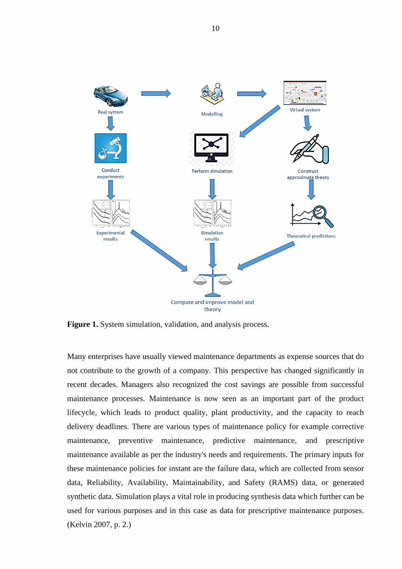
In the simplest form, a process for building a system simulation model and validating it with
a real system is shown in Figure 1. In a simulation, an actual system or component of a
system is investigated. The model is therefore a formulated based on an ideal description of
the system. This phase is often difficult and challenging since the modeler must select the
essential elements of the system because leaving out any essential elements leads to an
invalid model and adding redundant elements complicates the model. After modeling, an
appropriate simulation tool can be selected depending on the system requirements and level
of accuracy needed and simulation can be run to produce the simulation results. The model
validation is performed in the next step where the simulation result is compared with the
experimental data and theoretical prediction of the same system. The model validation
focuses on the detection and reduction of simulation model defects by comparing simulation
results from the model to the experimental results. The simulation model undergoes
continuous improvement until the model validation is successful and a clear conclusion is
drawn. This validated model now can be used in various ways to predict the system operation
by introducing changes in the inputs of the system. (Yin & Mckay 2018, p. 2-4.)
10
Figure 1. System simulation, validation, and analysis process.
Many enterprises have usually viewed maintenance departments as expense sources that do
not contribute to the growth of a company. This perspective has changed significantly in
recent decades. Managers also recognized the cost savings are possible from successful
maintenance processes. Maintenance is now seen as an important part of the product
lifecycle, which leads to product quality, plant productivity, and the capacity to reach
delivery deadlines. There are various types of maintenance policy for example corrective
maintenance, preventive maintenance, predictive maintenance, and prescriptive
maintenance available as per the industry's needs and requirements. The primary inputs for
these maintenance policies for instant are the failure data, which are collected from sensor
data, Reliability, Availability, Maintainability, and Safety (RAMS) data, or generated
synthetic data. Simulation plays a vital role in producing synthesis data which further can be
used for various purposes and in this case as data for prescriptive maintenance purposes.
(Kelvin 2007, p. 2.)
11
1.1 Motivation
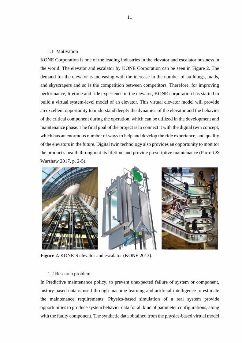
KONE Corporation is one of the leading industries in the elevator and escalator business in
the world. The elevator and escalator by KONE Corporation can be seen in Figure 2. The
demand for the elevator is increasing with the increase in the number of buildings, malls,
and skyscrapers and so is the competition between competitors. Therefore, for improving
performance, lifetime and ride experience in the elevator, KONE corporation has started to
build a virtual system-level model of an elevator. This virtual elevator model will provide
an excellent opportunity to understand deeply the dynamics of the elevator and the behavior
of the critical component during the operation, which can be utilized in the development and
maintenance phase. The final goal of the project is to connect it with the digital twin concept,
which has an enormous number of ways to help and develop the ride experience, and quality
of the elevators in the future. Digital twin technology also provides an opportunity to monitor
the product's health throughout its lifetime and provide prescriptive maintenance (Parrott &
Warshaw 2017, p. 2-5).
Figure 2. KONE’S elevator and escalator (KONE 2013).
1.2 Research problem
In Predictive maintenance policy, to prevent unexpected failure of system or component,
history-based data is used through machine learning and artificial intelligence to estimate
the maintenance requirements. Physics-based simulation of a real system provide
opportunities to produce system behavior data for all kind of parameter configurations, along
with the faulty component. The synthetic data obtained from the physics-based virtual model

12
can be used in machine learning and artificial intelligence to find the signature pattern for
the simulated case. Prescriptive maintenance is the combination of predictive maintenance
policy and physics-based simulation policy along with machine learning and artificial
intelligence to not only search for failure signature pattern but also gives information to
avoid or delay equipment failure. In order to implement prescriptive maintenance, greater
engineering effort is required as shown in Figure 3. (Aspentech 2021.)
Figure 3. Digital twin value chat (Edrmedeso 2020).
In principle, creating synthetic data from a physics-based virtual system appears to be a
straightforward approach, but in practice, it is not. Some of the greatest challenges in the
process are creating a sensitive and robust virtual model of the system, modeling of the
malfunction condition or component in the system and identification of the malfunction’s
signature pattern and many more.
1.3 Objectives and research questions
During the analysis of the model, the accuracy of the model behavior increases as the level
of detail increases but at some point, increasing the detail in the model has no longer an
effect on the results. Therefore, knowing the optimal number of the detail of the system is
required to build a generic model. Once the generic model is built, by changing important
parameters in this case travel distance, different masses, different stiffnesses, different
damper, etc. the entire family of the elevator can be analyzed.

13
The main objective of this project is to validate the computed results such as car position,
velocity, vibration, etc. obtained from the system-level model of the elevator with the data
collected from the measurements. The fulfillment of the requirement for this goal is obtained
by comparing the calculated and measured signals at the peak to peak value vibration and
should be when the load, speed, travel is maximum or minimum. The results should be in
the same range and the differences explicable. To gain further reliability of the model,
sensitivity analysis of different nominal run cases will be performed. Physics-based
simulations are becoming increasingly relevant as computer power increases. Simulations
are a viable alternative for getting synthetic data for product platform parameters
configurable scenarios. A preexisting physic-based simulation model of a KONE elevator
system from different platforms constructed prior to the thesis will be utilized as a reference
model for modeling the elevator system in the thesis. The second objective of this thesis is
to model the top three different load cases that occur in the elevator system which are listed
below.
1. Sag and bounce: - when the passenger getting in and out of the elevator car
2. Buffer run: - when the car does not stop at the lowest level and hits the buffers.
3. Counterweight run: -when the car does not stop at the top floor and the counterweight
hits the buffer.
The main research questions of the thesis are listed below.
How detailed a system-level model of an elevator is required to obtain the result
closed to the physical product?
Why the selected parameters are the most important ones while changing from one
elevator family to another without losing accuracy in the results?
How most common load cases in the elevator system can be modeled in the virtual
environment?
How synthetic data obtained from simulation can be used for prescriptive
maintenance?

14
2 METHODS AND METHODOLOGY
In this chapter, the importance of simulation in the implementation of prescriptive
maintenance is discussed. The methods which can be used for modeling and analysis of the
different elevator components are mentioned.
2.1 Maintenance policies and their primary requirements
Maintenance requires all steps possible to maintain or restore the correct operation of
equipment or machines. The aim is to eliminate the possibility of failures that can lead to
machine breakdown or unscheduled downtimes, or that could escalate to safety problems.
For example, wear, progressive damage, or material deformation due to force that develops
in several mechanical parts, for example, roller bearings, O-rings, or gears, is the common
cause of failure. Systematic maintenance processes improve machine availability, minimize
costs and encourage appropriate maintenance plans to be scheduled. Traditional, preventive
maintenance requires the routine monitoring of devices according to a set timeline or fixed
target based on the simplistic presumption that faults occur most of the time. However, this
strategy does not work most of the time for the reason being failure takes place before
planned maintenance or maintenance is performed even though it was not required.
(Centomo et al. 2020, p. 1782.)
2.1.1 Predictive maintenance
Predictive maintenance aims at solving the strategy of the fixed schedule by implementing
a procedure to predict specific possible failures. The purpose is to have maintenance unless
is really required, i.e., not too soon, or too late. Predictive maintenance has the benefit of
substantially reducing maintenance costs by allowing better use of capacities and preventing
operation downtimes. (Centomo et al. 2020, p. 1782.)
Predictive maintenance is focused on the prediction of faults based on the data collected by
different sensors, for examples vibration, temperature, humidity, or acoustic sensors. Thus,
it is important to preset data that describe the different states of the machine for example
location sensors or switches as well as the actuator status. Based on preset data and collected
data from the decision for maintenance are called out. Due to a large number of data

15
collection, manual tracking, and decision-making are impossible. That is why machine
learning and particularly deep learning are the best fit for data processing. They are often
used for predictive maintenance tasks like Remain Useful Life (RUL), Root Cause Analysis
also referred to as Fault Diagnosis (FD), Fault Prediction (FP), and Maintenance Strategy
Optimization (MSO). But before the use of the Machine Learning (ML) algorithm, all sets
of data labeled with the respective fault and patterns or shape of signals have to be
discovered. This data is then used as a source of information for predicting when which
failure has taken place. Figure 4 illustrates the predictive maintenance working processes
and various technologies use to accomplish an effective process. (Çınar et al. 2020, p. 8211;
Klein & Bergmann 2018, p. 3.)
Figure 4. Predictive maintenance working principle and used technologies (Çınar et al.
2020, p. 8211).
The collection of data and creating algorithms from machine learning in predictive
maintenance are the most challenging phase in the process. There are two approaches for
data collection described in detail in the next sub chapters, and many methods for application
of ML algorithm in predictive maintenance such as Artificial Neural Network (ANN),
Support Vector Machine (SVM), Decision Tree (DT), Random Forest (RF), Logistic

16
Regression (LR), Extreme Gradient Boosted Trees (XGBoost), Gradient Boosting Machines
(GBM), Linear Regression, Symbolic Regression (SR) (Çınar et al. 2020, p. 8211).
2.1.2 Prescriptive maintenance
Prescriptive maintenance works in cooperation with preventive maintenance and physics-
based simulation to indicate not only what and when a breakdown will occur, but also why
it will occur when the behavior of equipment had changed. Prescriptive maintenance will
take the study a step further by determining alternative choices and their potential effects in
order to reduce any harm to the system. The data and analysis will continue in the period
prior to the maintenance activity, with the potential consequences and suggestions being
continually adjusted and changed, increasing the credibility of the results. The analytical
engine will keep monitoring the machine after the maintenance activity is done to see if the
maintenance was effective. (Kovacevic 2017.)
A machine learning model that is developed on sensor and service data is required for
prescriptive maintenance to be successful. The artificial intelligence model would be
increasingly accurate when more high-quality data becomes available, recognizing more
indicators of maintenance requirements and failure signatures while providing fewer false
positives. During training a prescriptive maintenance algorithm, higher-level information
about an industry may be supplied to the machine learning algorithm. This allows the
program to consider important factors for example maintenance costs and product downtime.
The machine learning model is trained using specialized hardware, which might be local, or
cloud based. The model is code that may be installed on-premises or in the cloud, therefore
a means to reach and operate it is necessary. This can be readily connected with various asset
management software packages, easing the process of implementing the prescriptive
maintenance model's suggestions. At last, prescriptive maintenance needs a company's
willingness and ability to put into practice the machine learning suggestions. Hypothetical
outcomes created by a prescriptive maintenance program give options that were previously
either left by chance or tried and tested. (Aspentech 2021.)
In many sectors and industries, predictive maintenance has been proven to be accurate. A
company or organization's physical operations can benefit from the power of machine

17
learning by implementing prescriptive maintenance suggestions. The difference between
prescriptive maintenance and predictive maintenance is that prescriptive maintenance gives
a range of alternatives and outcomes from which to choose. In many cases, prescriptive
maintenance can also detect capital expenditure needs months before they could even appear
to human operators giving time to the company for economy purchases. (Aspentech 2021.)
2.1.3 Methods of data collection
The primary method for determining the health condition of machines is by observing the
machine which can be successfully achieved by the implementation of a sensor. The IoT
sensor such as accelerometers, gyroscopes, pressure sensors, etc. is normally used for this
process. The data coming from the sensor then can be utilized for the ML algorithms for
predictive maintenance. However, the implementation of these sensors is not straightforward
and vary many cases not appropriate especially for already existing machines and equipment.
The failure data of machines are generally collected by a method called run-to-failure. This
method can be very time-consuming and costly for larger sets of data. Once data has been
collected, there come difficulties for data handing and drawing conclusions that can be used
in predictive maintenance. (Centomo et al. 2020, p. 1786.)
Although there is not enough or sufficient data available for analysis from the actual system,
it is possible to generate them. There are four ways to generate the sensor data: fully
synthetical, synthetical based on previous data, synthetical based on a virtual simulation
model, and finally based on a simplified physical model (Klein & Bergmann 2018, p. 4).
For the generation of fully synthetic data, sensor data is produced using a parameter-based
algorithm. This method may slightly drift from its concept because its results are based on
the statical model. (Klein & Bergmann 2018, p. 5.) The procedure made by Hahsler et al.
can be used for generating and analyzing fully synthetic data (Hahsler et al. 2017, p. 1-45).
Generation synthetic data based on previous data can be archived by generating new data
based on fundamental properties of existing data distribution. This could be achieved by
preparing a generative and discriminative neural model by either directly learning the
distribution parameters or indirectly using a generative adversarial time-series network.
(Klein & Bergmann 2018, p. 5.)

18
Synthetical data generation based on a virtual simulation model uses a computer simulation
platform for creating a model with the property of the actual model which can be used for
data generation. An engineer can model faulty components or a variety of failure scenarios
by adjusting temperatures, flow rates, or vibrations or adding a sudden fault in the system.
These faults containing model can be simulation and results containing failure data can be
labeled and stored processed for further analysis. Many industries have used this approach
for creating virtual factory, machine health testing applications. (Klein & Bergmann 2018,
p. 5.)
Synthetical data generation based on a simplified physical model uses a similar approach but
instead of using a virtual model, it uses a simplified physical-based model. The models can
be replicated in two different ways. One using actual components which are used in real
machines and the other using not real components. The benefit of the second method is the
remarkably low cost of constructing such a model. Lego Mindstorms and Fischertechnik
(FT) provides such construction of the model at a low cost. (Klein & Bergmann 2018, p. 6.)
2.2 SimulationX - a system simulation software
SimulationX is a Multiphysics software tool based on Modelica (Modelica is a non-
proprietary, objects-oriented, multi-domain equations-based programming language that
may be used to simulate complicated physical systems) modeling language for modeling and
simulating of mechanical system, hydraulic, pneumatic, electro-material, control system,
along with thermal and magnetic systems. This provides great opportunities for simulating
and multi aspects of the model without unitizing co-simulation as shown in Figure 7. It can
be used to model, analyze, and optimize sophisticated, nonlinear, dynamic systems. The
graphic user interface of SimulationX software is shown in Figure 5. A user interface is used
to describe simulation models interactively. Domain-specific libraries contain ready-to-use
model components. SimulationX employs well-known symbols and input values. The user-
defined component can be constructed by assembling already available elements with
TypeDesigner. A model of component or system can be made through diagram view or 3D
view or text view. It also provides the opportunity to calculate the natural frequencies of the
model. It has a real physics element; thus, it can run in real-time. The great majority of
SimulationX applications are focused on drive systems, hybrid powertrains, mechatronics,

19
and vehicle dynamics. Furthermore, constructing the hoisting model (virtual prototype of an
elevator) and network modeling in SimulationX not only offers the user a realistic and
current engineering solution, but it also saves time and has a long lifetime. This technology
is also compatible with software like as Microsoft Word, Excel, and COMSOL.
(SimulationX 2016.)
Figure 5. Graphic user interface of SimulationX software (SimulationX 2016).
2.3 Method of modeling of electronics and control
In his chapter, the electrical motor modeling method and the controller modeling method for
actuating and controlling the elevator system are presented.
2.3.1 Electrical motor modeling
The dynamic modeling of the motor as a mathematical model based on voltage equation. For
instant, the voltage equations from motor modeling are listed below, which are based on Liu,
et al. work (Liu et al. 2015, p. 1121).
𝑢𝑑 = 𝑟𝑖𝑑 + 𝐿𝑑
𝑑𝑖𝑑
𝑑𝑡− 𝑝𝜔𝐿𝑞𝑖𝑞 (1)

20
𝑢𝑞 = 𝑟𝑖𝑑 + 𝐿𝑑𝑑𝑖𝑑
𝑑𝑡− 𝑝𝜔(𝐿𝑞𝑖𝑞 + 𝐾𝑒) (2)
Where 𝑢𝑑 and 𝑢𝑞 are voltage in axes 𝑑 and 𝑞 , r represents winding resistance in every
phase, 𝐿𝑑 and 𝐿𝑞 represents inductance axes 𝑑 and 𝑞, 𝜔 angular velocity of the mechanical
part, Ke is back electromotive force coefficient, p is motor pole pairs and 𝑖𝑑 and 𝑖𝑞 is current
in axes 𝑑 and 𝑞 (Liu et al. 2015, p. 1121).
The generation of the equation contains various assumptions and neglection such as the
model is linear regardless of the eddy current and hysteresis loss, neglecting the impact of
cogging and armature reaction, the winding is completely symmetrical in three phases (Liu
et al. 2015, p. 1121). An inverter can also be modeled to convert DC power to AC power
and desired sinusoidal or trapezoid signals can be produced as per request for permanent
magnet synchronous machine (PMSM). To connect the one-dimensional electrical parts
with the MBS part, the interface elements can be used.
2.3.2 Controller modeling
Controllers are made up of software and hardware that are designed to run algorithms rapidly
and efficiently. Such algorithms aim to increase the speed of complex transactions involving
mathematical and logical equations. This algorithm may either be hardwired into the
controller's structure or run as customized code on a microprocessor. Each digital control
system is optimized for the system it operates in order to maximize performance and achieve
the fastest response time possible. The control system is used to impose the position, speed,
and current of electric power on the elevator that enhances the precise and accurate response
of the elevator to position requirements. (Ford et al. 2016, p. 309.)
Figure 6 (a) shows the working principle of Cascaded control system. The position controller
is shown in figure 6 (d) where ϴm is position and Kpϴ proportional gain constant. The speed
controller is shown in figure 6 (c) where ωm is speed, KiΩ integral gain constant, KpΩ is
proportional gain constant, Ia is armature circuit, K is motor constant, Tem is motor torque,
Jeq is equivalent inertia of the motor, load and pulley and current controller is shown in figure
6 (b) where Ra is armature resistance, kpI is the proportional gain, kiI is integral gain, Vc(s) is
control voltage, kPWM is 4-quadrant Pulse-Width-Modulation converter, Va(s) is voltage Te

21
torque. These controllers are working together with three cascaded loops by utilizing the
motor position sensor and current output. Feedback controllers are designed to regulate a
system accurately and rapidly based on real-time feedback received from the system
themselves, with no need for external adjustment. A correctly built control scheme can
reduce a process's steady-state error to zero in a short period with little oscillations and
minimal overshoot. Proportional-Integral (PI) controller corrects gap between desired and
measured speed or current with respect to the given proportional and integral values and
Proportional (P) controller that will properly adjust errors in the location of the drive. (Ford
et al. 2016, p. 310.)
Figure 6. Cascaded control system (a), controlled loops for current (b), speed (c) and
position (d) (Ford et al. 2016, p. 311).

22
The elevator controlled are consists of motion controller, PI controller and controlled
inverter. The motion controller determines the required velocity for the PI controller
depending on the current position, velocity, and desired floor. The PI controller will
determine how much torque is needed depending on the difference between the intended
elevator velocity (from motion controller) and the present elevator velocity. The inverter
controls the machine's electric phases by establishing an initial set of currents. A coordinate
transformation of the machine into a direct quadrature zero (dq0) representation is used for
this control. The control then comprises many components, including a PI controller for the
currents d and q with the specified gain calculated by the inductance Ldq and specified in the
parameter.
2.4 Functional mock-up interface and co-simulation
Functional Mock-up Interface (FMI) is an autonomous platform for the sharing of models
and simulation of complex models using a mix of XML files and compiled C-code. FMI
contains a series of basic functions for exchanging data and synchronizing sub-systems in
interaction stages. These sub-systems are referred to as FMI slaves, while the co-simulation
supervisor is referred to as FMI master. This provides an opportunity to have the same model
simulation in different platforms for different analyses and therefore investment in a model
portfolio significantly increases. (Modelon 2020.)
Functional Mock-up Unit (FMU) is a file that includes a model of simulation complying
with the FMI specification (with the extension.FMU). FMUs are divided into two categories
by the FMI standard: model exchange FMUs use differential equations to describe
dynamical processes. The FMU must be connected to a numerical solver in order for the
model to be simulated. The solver decides the phase size and how to calculate the state at
the next time step after setting the FMU internal state and asking for the state derivatives.
The other FMI standard is co-simulation where FMUs have their built-in numerical solver.
The import tool selects the inputs for FMU, orders the FMU to go further to the given time,
and reads the results for FMU after that point. (Modelon 2020.)
Co-simulation is a technique where one aspect of the model for example physical model is
combined with another aspect for example mathematical model to perform a simulation
giving a deep level understanding of an entire system as shown in Figure 7. This technique

23
also can be used for studying multi-physical models where for example rigid bodies are
modeled on one platform and flexible bodies or acoustics or CFD or structural are modeled
on other and are coupled together to capture the system behavior in detail. This approach is
suited for the test of mechanical design, device specifications, system compatibility analysis,
and control system testing. (Baobing & Baras 2013, p. 71; Brezina et al. 2011, p. 59.)
Figure 7. Co-simulation of entire system (Brezina et al. 2011, p. 59).
SimulationX software is used for simulation of electrical, mechanical and controller all in
the same platform explained in detail in section 2.2. This platform also provides a facility
for co-simulation with another aspect if required. FMU technique has been utilized to import
a real motion control algorithm for the elevator. The Initial motion control algorithm is in
MATLAB Simulink Which is exported using FMI Co-Simulation Target for
Simulink®CoderTM. It allows to export MATLAB Simulink functions as FMUs and
reimport them into SimulationX. Especially for the FMU import behavior, some parameters
can be edited on the pages “FMI Settings” and “Master Algorithm” in SimulationX.
2.5 Principles of a multibody system
According to Flores ( 2015, p. 1). “a multibody system encompasses a collection of rigid
and/or flexible bodies interconnected by kinematic joints and possibly some force elements.”
The method of multibody system dynamics can be described as an efficient way of studying
such mechanical systems. This method is extremely successful for mechanical systems
which contain several bodies interconnected with mechanical joints as shown in Figure 8.
Examples of the use of multibody structures, including automotive vehicles, mechanisms,

24
robots, and biomechanical systems. Recently, there has been a significant rise in the
application of this multibody system dynamics approach to analyze the mechanical structure.
(Flores 2015, p. 1-2.)
Figure 8. Multibody system representation (Flores 2015, p. 2).
There are several techniques to formulate equation of motions for computational multibody
dynamics. Some techniques allow producing motion equations in a differential-algebraic
equations whereas some in a minimum group of basic differential equations and a number
other intermediate approaches offer different alternatives as shown in Figure 9. Depending
on application and priorities, each formula has its own benefits and restrictions. (Flores 2015,
p. 3.)
The most basic method of generating equations of motion is with a large set of differential-
algebraic equations. A group of translation and rotational coordinates defines the structure
of a rigid body. To describe kinematic joints between bodies, algebraic constraints are
implemented, and then the Lagrange multiplier technique is used to define joint reaction
forces. This formulation is called body-coordinate formulation. Body coordinate formulation
is also called as the absolute coordinate formulation or Cartesian coordinate formulation.
While these formulations are simple to build, one of the key disadvantages is their
computational inefficiency. These types of formulations are adopted in many commercial
multibody simulation software such as ADAMS and DADS. This formulation method is

25
employed to the generation of dynamic analysis of the multibody system in this thesis.
(Nikravesh 2004, p. 83.)
The other formulations of equations of motion are point-coordinate (or natural coordinates)
formulation and joint-coordinate formulation. The point coordinates formulation method is
based on the constrained Newton equations therefore the rotational coordinates are excluded.
In joint coordinates formulation, relative coordinates and velocities are used and it results in
much fewer sets of equations. Through a systematic method, these equations are obtained
by translating the body-coordinate formulation to the joint space. (Flores 2015, p. 7.)
Figure 9. Most commonly used coordinate types in Multibody system (Flores 2015, p. 7).
2.5.1 Coordinates system
Global and local coordinate system is used in the formulation of multibody spatial system.
The global coordinate system is to define the frame of inertia and the local coordinates
system is to define the local properties of points belonging to a particular body. The local
coordinates systems translate and rotate with the motion of the body and, therefore, its
position and rotations differ with time. The method of translating local coordinate into global
coordinate is defined by a transformation matrix. (Flores 2015, p. 11-12.) The description of
the position vector and local coordinates can be seen in Figure 10.

26
Figure 10. Description of the position of a point in the spatial body (Flores 2015, p. 12).
There are numerous methods in spatial multibody systems for defining the rotational
coordinates such as Euler angles, Bryant angles, Rodrigues equation, and Euler parameters.
Each method has its own advantages and disadvantages. Sometimes a combination of two
separate rotation representation processes could be used to get the best output. Details
information can be found in (Flores 2015, p. 11-12).
2.5.2 Generalized coordinates
Generalized coordinates are classified as a collection of convenient and typically
independent coordinates for the purpose of explaining the configuration of a specific system.
The quantities of independent generalized coordinates determine the number of degrees of
freedom of the system if external constraints are applied to the system then that results in
some dependence among the generalized coordinates. For example, if a specific
configuration is represented by n generalized coordinates and m constraint equations (m<n),
the difference n-m is equal to the system's total degrees of freedom (DOF). Various terms
for velocity, acceleration, and equation of motion are required to be produced for the study
of multibody dynamics. The number and type of generalized coordination rely on the
selection of the kinematic description of the system. Therefore, to achieve a simple
expression for the velocity, acceleration, and motion equation, it is necessary to choose the
appropriate generalized coordinates. (Amirouche 2006, p. 46.)

27
2.5.3 Constraint equation
In multibody system modeling, the constraints indicate a restriction on one or more bodies’
kinematic degrees of freedom. In other words, mechanical joints are expressed through
constraints equations and are linked to generalized coordinates. Therefore, the constraint
equations impose the dependency in generalized coordinates. The constraint equations are
functions of the generalized coordinates and, in some cases, time. In general, the number of
generalized coordinates is higher than the number of constraints equations. (Amirouche
2006, p. 45-48.)
The kinematics constraints are classified into two categories namely holonomic and
nonholonomic. If the constraints depend on generalized coordinates and possibly on time
then it is called holonomic, otherwise, it is nonholonomic. The holonomic constraints in the
multibody system are further divided into two categories that are, scleronomic and
rheonomic. If constraints do not include time as an explicit variable, they are called
scleronomic and if constraints are a function of time, they are called rheonomic. The detailed
kinematic equation formulation based on the vector of body coordinates can be shown in
(Flores 2015, p. 31-35).
Modeling of the joints is an essential step during the study of multibody dynamics. In a
multibody system, multiple bodies are linked with joints. Joints also provided restrictions to
the relative motion of the bodies. There are various types of joints in mechanical systems.
The various joints type minimizes the number of DOF in the system. Revolute joints,
translational joints, spherical joints, cylindrical joints, screw joints, and planar joints are
commonly used joints during the modeling of the multibody system. These basic joints are
being used to establish joints with different mechanisms. (Flores 2015, p. 7.) Complicated
joints can be constructed utilizing a combination of several types of simple joints. The
formulation of the kinematic joint constraints for the spherical joint, revolute joint and the
spherical-spherical joint is shown in (Flores 2015, p. 43-48). Different properties of different
types of joints can be seen in Table 1.

28
Table 1: Joint types and total DOF (Mathworks 2021).
Joint Type Total DOF Restriction of
Translational DOF
Restriction of
Rotational DOF
Revolute 1 3 2
Spherical 3 3 0
Translational 1 2 3
Universal 2 3 1
Fixed 0 3 3
Cylindrical 2 2 2
Prismatic joint 1 2 3
Bearing joint 4 2 0
2.5.4 Dynamic analysis of multibody system
The dynamic equation of motion can be derived from different techniques. The dynamic
analysis of the system includes determining dynamic equilibrium and dynamic equilibrium
can be represented by second-order differential equations. If the system is unconstrained, the
equation of motion could be formed with Newton-Euler equations. If the system is
constrained, there are several other processes to solve the equation of motion of spatial
multibody systems namely Lagrange multiplier method, the Embedding technique, the
Baumgarte method, the penalty method, and the augmented Lagrangian formulation. (Flores
2015, p. 61.)
In the augmented formulation, the dynamic equations appear with constraint forces and are
represented as redundant coordinate. For unknown accelerations and constraint forces, the
constraint relationship is used with the differential equation of motion. In this process, a
sparse matrix structures are formed. The augmented formulation, however, has the downside
of rising the dimensionality of the problem and, needs father advanced numerical algorithms
to calculate the resulting systems of differential and algebraic equations. (Flores 2015, p.
61.)
The Lagrangian dynamics are based on a higher systematic and universal method for
designing the augmented equation of motion. The Lagrange multiplier technique is utilized
in the Lagrangian method to describe generalized constraint forces and to generate an

29
augmented formulation where the coefficient matrix is symmetric. In the formulation of the
augmented equation of motion, Lagrange multipliers are mostly used. There are equal
number Langrage multipliers and constraints equations in the system. This equation has
constraints in terms of acceleration and the constant equation vanishes after differentiating
the constraint equations two times with respect to time. Therefore, to overcomes this
downside, a constraint stabilization method for example Baumgarte stabilization method, a
penalty formulation or an augmented Lagrangian method can be introduced. Figure 11 shows
the algorithm for dynamic analysis of multibody systems on the basis of the standard
Lagrange multipliers method. (Flores 2015, p. 60-68.)
Figure 11. Flowchart based on the standard Lagrange multipliers method for dynamic
analysis of multibody systems (Flores 2015, p. 63).
2.5.5 Collision and contact modeling methods
When studying a real multibody system, contact modeling is an important modeling aspect.
Contact modeling's main feature is to detect the collision point and give the reactions of the
collision. It is also used to evaluate the contact forces between two bodies. Two
computational methods, named finite element analysis (FEM) and multibody system (MBS)
can be used to perform contact analysis. FEM is the most effective content analysis tool and
compared to MBS, the results are very accurate, but takes longer processing time. In this

30
project, the collision and contact modeling will provide the results of the buffer crash of the
elevator car and counterweight. (Baharudin 2016, p. 41.)
There are two key stages in contact modeling i.e., collision detection and collision response.
The detection of collision’s time and the location is accounted in the collision detection
model whereas, the contact force between the two bodies is accounted in the collision
reaction model. Since the protocol must be carried out in real-time, a correct contact
algorithm must be used to decide the time and location contact takes place and computes the
contact response. (Baharudin 2016, p. 42.) One can see in Figure 12 below, the general
algorithm for contact detection and content response models.
Figure 12. Contact detection and content response modeling algorithm (Baharudin 2016, p.
42).
For the collision detection between two geometrically different bodies, bounding volume
(BV) techniques can be used. This approach functions to estimate when bodies intersect and
utilize spheres or boxes that summarize the complicated geometrical entity into a simple
form as shown in Figure 13. The collision detection mechanism can be greatly enhanced
using these simple forms. For collision detection, a variety of bounding techniques may be
utilized, like Axis-Aligned Bounding Box (AABB), Discrete-Orientation Polytope (k-DOP),
and Oriented Bounding Box (OBB) (Baharudin 2016, p. 41).

31
Figure 13. Bounding box approach for contact modeling (Baharudin 2016, p. 42).
For collision response, many techniques, for example, penalty methods, analytical methods,
and impulse methods, can be used. Penalty methods are the technique in contact modeling
that enables minor penetrations among bodies at the contact point and these are considered
as soft contact. With the spring-damper components, the penetration interval is integrated.
The contact force is measured and introduced in the equation of motion as an external force.
In the analytical methods, the contacts are solved with the constraints which lead to the
addition of an extra dimension to the equation of motion and contribute to the computational
expense. In the impulse methods, the contact forces of colliding bodies are not computed,
and instead, the velocities at the contact point are computed and introduced directly to the
bodies. (Baharudin 2016, p. 42.)
The kinematic of the contact point can be represented with the help of Figure 13. Multibody
formulations can be used to determine the position of the two points. The two-point are i and
j, the distance between them is 𝐝𝑝, is expressed below (Baharudin 2016, p. 43).
𝐝𝑝 = 𝐫𝑗 − 𝐫𝑖 (3)
The n normal vector of the contact is expressed below (Baharudin 2016, p. 43).
𝐧 =𝐝𝑝
‖𝐝𝑝‖ (4)

32
The normal magnitude between two points 𝑑𝑝 is determined below (Baharudin 2016, p. 43).
𝑑𝑝= 𝐧T𝐝𝑝 (5)
By differentiating equation (5) with respect to time, the relative normal velocity 𝑣𝑛 between
two points can be determined below (Baharudin 2016, p. 43).
𝑣𝑛 = 𝐧T(𝑗 + 𝑖) (6)
When a collision takes place, a spring-damper is applied at the contact point to identify forces
of contact and 𝑑𝑝 becomes as penetration distance at the contact point. The normal contact
force, 𝐅𝑛 at the contact point is expressed below (Baharudin 2016, p. 43).
𝐅𝑛 = −(𝐾𝑑𝑝 + 𝐶𝑣𝑛)𝐧 (7)
Where K is the coefficient of the stiffness and C is the damping factor (Baharudin 2016, p.
43).
2.5.6 Rope modeling methods
Wire ropes are commonly used in various engineering areas because of their excellent
mechanical characteristics and comprehensive applicability. Wire rope is used extensively
in the hoisting industry; thus, it is necessary to anticipate the consequences of using wire
rope. Generally, wire rope experiences the combined force conditions of tension, bending,
contact, friction, impaction, and vibration. It is difficult to explain the stress progression and
deformation of the cabling at the operating phase because of the dynamic loading state. Thus,
many researches had been conducted by constructing a mechanical model of wire for
understanding stress analysis, failure mechanism, mechanical properties, and lifetime
predictions. (Huang et al. 2018, p. 37.)
The principle of wire rope with respect to the behavior of deformation and strength under
different loading conditions has been discussed in detail. Multiple contributions are made
for non-linear static and dynamic finite element and multi-body simulations of spatially

33
discrete cable models. The most common approach for modeling wire rope is as a series of
elastic links, connected by spherical joint (Spiegelhauer & Schlecht 2020, p. 68). Figure 14
shows the modeling method of cables. Linear finite element models use straight elastic
elements to link individual particles or lumped masses and finite segment models consist of
rigid elements joined by spherical joints. These models usually ignore the bending stiffness
of the wire, excluding finite segment, model torsional spring at the joints. For modeling
cable-pulley structures, nonlinear finite element models are common. The continuous
existence of the formulations of curved elements is beneficial since the contact forces could
be described as continuous functions of the cable position and velocity. It has been possible
to simulate the cables without pre-tensions or under compressions with high order non-linear
finite elements. In the multibody simulation, if the wire rope is experiencing large
deformations, then the non-linear dynamic behavior can be studied by the absolute nodal
coordinate formulation (ANCF) method. (Westin 2018, p. 3.)
Figure 14. Modeling methods of cable (Westin 2018, p. 3).
The rope and pulley available in SimulationX software are based on the mechanics MBS
domain. The rope is models as a rope spring which symbolizes a free rope section or strand
for the analysis of longitudinal rope oscillations. Internally, it is discretized into masses and
spring-damper and this element evaluates stiffness and damper forces between the
connection points. The rope, pulley and drum models are grouped in to ready to use pulley
and drum.

34
3 ELEVATOR ARCHITECTURE
The components of real elevator systems are introduced first, followed by virtual modeling
of each elevator system component in SimulationX software. At last, the modeling of three
load case situations of the elevator system is present.
3.1 Real elevator system
An elevator is a machine to transfer people and objects vertically, in other words, called as
“vertical people’s transportation system”. The use of elevators is not limited to high-rise
structures but also applies to low-rise structures. From manual hoisted elevators to traction
sheave elevators, they have evolved with time. Elevator cars are suspended from one end of
the rope and counterweights are attached to the other end of the rope. All elevators use
traction-based hoisting mechanisms. They help to balance both the cars and their riders, as
well as providing enough traction to prevent ropes from slipping off of their loop. Figure 15
represents the elevator and its basic components.
The Elevator motor (E-machine) is the power source in the elevator system. KONE uses
motor named EcoDisc© which is a gearless permanent magnet synchronous machine
developed by KONE corporation back in 1996. This is the first room-less (MRL) elevator
drive built to position the motor in the guide shaft. This motor offers several advantages,
including improved material and energy economy, the absence of oil, frequency control, and
low friction gearless design, all of which contribute to consume just half the power needed
by equivalent traditional systems. Steel rope travels through the drive pulley and the wire
tension is given by the weight of the hanging car and counterweight. Suspension ropes
convert the work done by the machinery into the movement of the car. When these ropes
travel over the traction sheave, they are moved by friction between the ropes and sheaves.
(Ford et al. 2016, p. 308.)

35
Figure 15. Elevator and its components.
E-machine is controlled by electric drives called a controller. Depending on the input current
and voltage, the control system operates the E-machine at varying torque and speed levels.
Electricity and communication between passengers such as selection of floor are supplied to
and from the elevator car employing traveling cable to the controller. The controller is
located at top of the shaft and the traveling cable is connected to the car's bottom while
enabling unrestricted car movement.
The elevator car is that which travels vertically to transport passengers from one floor to the
other. Elevator cars are either firmly connected to a sling or utilizing springs and dampers.
The sling is a frame assembly that wraps around the elevator car and is supported by
suspension ropes and guide rails. It serves as the car's main support framework. The Pulley

36
beam is part of the sling allocated at the bottom of the car, where spring or dampers are used
to minimize vibrations coming from suspension ropes.
Guide shoes are used to ensure the contact of the car to the guide rail throughout the travel.
There are four guide shoes, two on each side of the car. There are two types of guide shoes
i.e. roller and sliding guide shoes. The use of roller or sliding guide shoes is dependent on
the quality of ride requirement or speed for that elevator. Roller guide shoes have lower
friction for rolling contact over sliding contact. Sliding guide shoes uses oil as a lubrication
agent to lower the friction. Typical roller guides employ damping material or springs to
absorb the vibration, but due to higher comfort standards, active and passive dampening
mechanism are now used to decrease lateral elevator vibrations, particularly in high-rise
buildings. (Kheir 2015, p. 1085.)
Car guide rails and counterweight guide rails are used to ensure a car and counterweight
traveling in a straight line. They are firmly attached to the shaft walls with brackets and to
each other with fishplates. To provide a smooth and comfortable ride, guide rails should
always be installed accurately. (Ishii 1994, p. 44.)
The elevator system consists of two types of doors. Car doors that are attached to the elevator
car and move with it. Every landing floor has a landing door. When the elevator is traveling,
both doors are shut to protect people from dropping down. Passengers can securely enter and
exit the elevator when it reaches the landing floor.
Overspeed governors (OSG) are speed monitors that check elevator speed and, if it exceeds
the allowed limit due to anomalous acceleration, activate safety mechanisms and put the
elevator to a safe stop. If the electrical Overspeed governor fails to stop the car, a mechanical
safety device kicks in and is activated by clutching the guide rails tightly and bring the car
to a stop.
Elevator systems also consist of buffer at the bottom of the pit under the car and under the
counterweight. It provides added safety to the passenger in case the car won’t stop at the
landing floor and run the pit. At buffer impact, buffer absorb and disperse the kinetic energy
of the falling elevator and lessen the falling impact´s force.

37
3.2 Modeling of an elevator system
The modeling of the elevator at the system level has been done in SimulationX software.
The development in the model of the elevator has been carried out in sense to capture
position, velocity, vibration, motor torque, guide shoes forces, along with many other
phenomena of different components in the spatial direction. The most significant
components contributing to the dynamic and electric behavior of the elevator are modeled
separately as components. These elevator components models are already available in
KONE’s library. A simplified representation elevator system and modeled components are
shown in Figure 16. The SimulationX model for the elevator system is presented in Figure
17.
Figure 16. Simplified elevator system.
Buffer

38
Figure 17. Elevator system model in SimulationX (1) controller, (2) motor, (3) motor
mount, (4) rope, (5) rope fixation, (6) pulley beam, (7) car mount (damper pad), (8) guide
shoes, (9) car, (10) counter weight, (11) buffer, (12) overspeed governor, (13) brake
actuation, (14) white noise.
Controller (1, Figure 17) modeled includes motion controller, PI feedback, feedforward, and
normalization based on method discussed in section 2.3.2. Motion controller has been
imported in the mode with FMU as discussed in section 2.4. The motion controller's main
inputs are floor request, car vertical position, and velocity of the car. Based on these inputs,
the motion controller calculates the desired car velocity trajectory. The desired velocity
trajectory is fed into the PI controllers where it continuously calculates the difference
between required vertical velocity set by the motion controller and measured vertical
velocity which comes from the measured rotational speed of the electric motor. PI corrects
this difference with respect to the proportional and integral values provided. This corrected

39
required vertical velocity is added with the feedforward controller where it calculates the
static load based on mass different results and the dynamic load based on the system mass
results to give static torque and dynamic torque. In the normalization part, the scale output
of the required torque is calculated.
The motor (2, Figure 17) contains electrical as well as mechanical components as discussed
in section 2.3.1. The mechanical component such as traction sheave, the mass of the motor,
degree of freedom limitation was modeled with the MBS methodology and the electrical
part’s contains axial flow synchronous machine, and modeling is done with the mathematical
formula for the voltage equations of PMSM. Motor mount (3, Figure 17) is modeled as the
3-dimensional (3D) spring with stiffness and damper properties. The stiffnesses used for
motor mount are calculated from the Finite elements method (FEM) analysis with 12 kN
load on the shaft. Translational and rotational stiffnesses are used to mount the motor at top
and bottom positions. The bottom mount represents the motor bed plate where the motor is
assembled with a damper pad. The bed plate is vibrating with eigenfrequencies of 17,9 Hz,
20,25 Hz, 24,63 Hz 26,31 Hz, 28,71 Hz and 53,21 Hz. The damping value has been obtained
from a similar component.
The ropes (4, Figure 17) in the system are modeled as rope elements as mentioned in section
2.5.6, and their primary inputs as linear density, axial stiffness and damper, and number to
ropes. The length of the rope on either side of the car and counterweight are model as the
position of the car and counterweight depended. Rope fixation (5, Figure 17) is modeled
with a prismatic joint allowing a vertical degree of freedom and stiffness and damping value
to represent the connecting point. The stiffnesses used in rope fixation are calculated from
the Finite elements method (FEM) analysis and the damping value has been obtained from
a similar component.
The pulley beam (6, Figure 17) is modeled with MBS-bodies and pullies with pulley element
with its point masses, the center of gravities and inertia of tensors, and positioned to represent
the skewed pully beam. The car mount (7, Figure 17) is modeled as a linear 3D spring to
represent elastic behavior and positioned under the car and pulley beam. With the correct
stiffness and damping ratio of these springs, a true damper can be represented in the model.

40
The stiffnesses utilized for car count are computed using the FEM, and the damping value
is acquired from a similar component.
Guide shoes (8, Figure 17) are modeled with a 1-dimensional spring and damper to represent
the contact point of guide shoes and guide rials in x-axis and y-axis. The same model of
guide shoes is used to represent roller and sliding guide shoes. The stiffness used for roller
guide shoes is obtained from the force-displacement curves of FE analysis for 1 mm
displacement to the compression force. For roller guide shoes, the stiffness value is the same
in both x-axis and y-axis direction however for the sliding guide shoe, the stiffness value is
different in both x-axis and y-axis direction and has a higher friction coefficient value. The
stiffnesses used for sliding guide shoes are as the measure in the lab for the load-deflection
test, and the result is found to be nonlinear. The current modeling structure in SimulationX
supports only linear spring constants, and thus a linear estimate is given for x-axis and y-
axis stiffness values. The damping value is acquired from a comparable component.
Guide rails are modeled as a function of the guide rails misalignments in form of curves
through with the excitation for the guide rail shoes are provided. The measurement of the
guide rail misalignment is a complicated procedure due to the compact arrangement of the
elevator system. Therefore, the modeling strategy is to scale the values of measured
misalignments, so they cover the entire available database of measured guide rails
misalignments with automatic adjustment tool (AAT).
Initially, the elevator car (9, Figure 17) has been modeled as a rigid body with MBS-bodies
which included car door and sling, with point masses, centers of gravity, and inertia of
tensors with respect to their position. The door and car were rigidly connected and at the
end, the entire car component could have 6 degrees of freedom. With this car model, the
vertical vibration accuracy was compromised and was not accurate enough for capturing the
local modes of the car. Therefore, a flexible car was introduced and discussed in the next
subsection. Counterweight (10, Figure 17) is modeled similarly to a rigid car and with a
pulley element.
Buffer (11, Figure 17) is modeled by simplifying the real components. The modeling is based
on a polynomial buffer force description where the seven degrees of the polynomial is used.

41
Visualization of the buffer is a rubber pad. Position of buffer contact and buffer characteristic
has been applied as per specification and as output, deflection, combine buffer force, spring
force, and damping force can be plotted. Over speed governor (12, Figure 17) is modeled
based on detecting car speed and provide elevator safety brakes when the speed of the car is
over the limit. Brake actuation (13, Figure 17) is a model based on safety gear signal. Delays
and brake force characteristics are taken into account. If safety gear is activated or if the
buffer gets in contact with the car, time count and time-dependent brake behavior is
activated. Time can be set for the break to be released and the elevator motion to begin in
the break release element.
The motor is modeled as an ideal motor as mentioned in section 2.3.1, which means that not
all the excitations from torque ripples, bearings, manufacturing tolerances are represented.
To overcome this simplification, white noise (14, Figure 17) is used as an initial excitation
of the motor. This will provide initial excitation to the motor. Idealities in modeling car,
hoisting components (guide rails, ropes, guide shoes), air pressure in the shaft, etc. reduce
scientifically the excitations transmitted to the car component. For this reason, the car is
excited with white noise, in order to see if during the ride any resonance may be built on.
The white noise signal is applied as a body force element to the motor mass and car mass in
3 spatial directions.
The geometrical information of the entire elevator has been collected from the Computer-
Aided Design (CAD) files and elevator installation layout. The masses, center of gravity and
inertia tensors are taken from Creo model of respective components.
3.2.1 Flexible car modeling
In flexible car modeling, the car’s roof and floor are modeled separately, and the entire car
including the sling door and in-car load is divided into two components as shown in Figure
18. The car is then joined via joints and springs providing flexibility to the car. The springs
connecting the components can be tuned to the FE computed eigenfrequencies of the roof
and floor. In this way, the local mode of the car can be implemented in the model.

42
Figure 18. Flexible car model.
A separate study for frequency response analysis was done to compute in-car
eigenfrequencies excited during car movements and induce in-car vibrations. FE method has
been used for this study utilizing Abaqus software. Eigenfrequency extraction with Lanczos
solver for frequency range 0,3 – 150 Hz has been used. The geometrical specification,
material data and connection between subsystem is made as per elevator car. During that
frequency analysis, the elevator car was attached to the ground through the guide shoes and
pulley beam mounting stiffness and analysis was done in static condition. The loading force
of 10 N has been applied in the vertical direction, on the bottom of the sling. Significant
vertical response of the car floor and roof for vertical excitation with 10 N has been expected
as a result. No damping was used during the analysis.
In the simulation model, frequency obtained from frequency response analysis is given to
the floor and roof of the car to capture local modes and potential resonances, through fine-
tuning the stiffness value of spring joining two parts of the floor and roof of the flexible car.

43
The correct stiffness value of spring could be obtained by multiple iterations of the stiffness
value of spring joining two parts of the floor in the SimulationX software. Figure 19 depicts
the influencing stiffness values for eigenfrequency tuning. The translational and rotational
stiffness is necessary to be estimated.
Figure 19. Influencing stiffness values
Bending mode comes mainly from rotational stiffness around the z-axis (kr_z). Due to the
kinematic assembly of two rotational joints, floorL and floorR can move independently
in translational y-direction shown in Figure 19. Movement is dependent on kt_y
(Translational y-direction) and leads to outer phase mode (no bending mode). The frequency
of this must be shifted outside the interesting frequency range (<150 Hz). Translational x-
direction (kt_x) is not constrained during flexible car model as it is necessary for squeezing
effect of car, thus must be restricted by kt_x and must be set appropriately.

44
kt_x can have too high an influence on lateral vibrations which is not wanted. If rigid
behaviour is wanted, one could set value infinite high which leads to extremely high
eigenfrequency and however, that leads to decrease of performance (simulation time)
therefore appropriate value kt_x is necessary which should shift eigenfrequency
(longitudinal vibration mode) outside interesting frequency range and can be calculated by
formula mentioned below.
𝑘𝑡𝑥 ≥𝑚𝑇𝑜𝑡𝑎𝑙𝜋
2𝑓2
2 (8)
Where 𝑚𝑇𝑜𝑡𝑎𝑙 is the total mass of the car and f is the lower limit for the eigenfrequency e.g.
f = 200 Hz.
This calculated value should be input in the simulation model for floor and roof and its
influences much be checked and if eigenfrequency is too low then the stiffness must be
adjusted.
The bending mode of the roof can be obtained analytically for estimation kr_z (rotational
stiffness around z-axis) however for floor stiffness simplified model of car damper pad and
pull beam should be used. This is because, in this platform models, damper pads have an
influence on floor bending mode. The roof and floor estimation formula are mentioned
below.
• Estimation roof stiffness
𝑘𝑟𝑧 = 2𝜋2 ⋅ 𝑓2 ⋅ 𝐽∗ (9)
• estimation floor stiffness
𝑘𝑟𝑧 ≤ 2𝜋2 ⋅ 𝑓2 ⋅ 𝐽∗
(10)
Where 𝐽∗ = 𝐽𝐹,𝑝𝑎𝑛𝑒𝑙 +mFloor
32⋅ 𝐵𝐵2 or 𝐽∗ = 𝐽𝑅,𝑝𝑎𝑛𝑒𝑙 +
mRoof
32⋅ 𝐵𝐵2
Where 𝑘𝑟𝑧 is rotational stiffness around z-axis, 𝐽𝐹,𝑝𝑎𝑛𝑒𝑙 and 𝐽𝑅,𝑝𝑎𝑛𝑒𝑙 is inertia for one panel
floor and roof, the value taken from SimulationX (in Centre of mass), mFloor is mass value
for the entire floor, BB is Internal width of the car

45
From this approach, the upper limit will be obtained therefore choose a lower value for cars
and iterate to matching eigenfrequency via eigenfrequency Analysis in SimulationX.
The same value obtained for the Kt_x can place here but this led to too high stiffness and
may lead to performance issues. Therefore, its own value should be determined as mentioned
below.
𝑘𝑦 ≥4
𝐵𝐵2⋅ (2𝜋2𝑓2 ⋅ 𝐽∗ − 𝑘𝑟𝑧) (11)
Where 𝐽∗ =𝐽𝐹,𝑝𝑎𝑛𝑒𝑙
2+
mFloor
32⋅ 𝐵𝐵2 or 𝐽∗ =
𝐽𝑅,𝑝𝑎𝑛𝑒𝑙
2+
mRoof
32⋅ 𝐵𝐵2
By following the above-mentioned procedure, the stiffness value can be calculated and tuned
to any wanted eigenfrequency of the floor. However, during the tuning of the
eigenfrequency of the floor at 81 Hz, its rotational stiffness value around x-direction krz is
calculated to be 100 Nm/deg at the frequency of 83,9 Hz. This value for rotational stiffness
value is significantly small and this also limits the tuning of floor eigenfrequency lower than
84 Hz. While looking at the potential energy distribution at this frequency, it is found that
the damper pads have a high influence and store higher potential energy as shown in Figure
20. In reality, the damper pads have an influence on floor eigenfrequency but should not
limit the eigenfrequency, therefore this issue must be overcome.
Figure 20. Potential energy distribution at 84 Hz floor frequency.

46
There are two ways to achieve the higher rotation stiffness value and be able to tune even
lower frequency than 81 Hz of the floor. By increasing the mass of the floor. This means
including the overall structure of the floor (i.e. floor and sling beam) till now only floor
masses are used. However, this is a case-specific solution and will be applied for this thesis
work to get going. The rotational stiffness value, in this case, is 1300 Nm/deg which still is
the small value and the involvement of damper pads are still high. The other option is by
changing the connection of damper pad from the floor of the car to the rigid frame of the car.
This involves a big model change hence further investigation is required to see its effect on
the other components and their results. For this reason, this option is not used during this
thesis work. The elevator components along with inputs are needed for the SimulationX
elevator model as presented in Table 2.
Table 2: Elevator components and their inputs required for modeling in SimulationX
COMPONENTS INPUTS
Car Dimensions, load, mass, center of gravity, the inertia of
tensor, type of car isolations and positions, eigenfrequency
of floor and roof, etc.
Sling Mass, the center of gravity, inertia of tensor, positions of
pulley beam, guide shoes, buffer counterpart, traveling
cable, compensation chain, interface car-sling (stiffness and
damper), etc.
Door Mass, type, the position of the center of mass in relation to
the car
Guide shoes Type, stiffness, damper, end stops clearance, friction
Counterweight Type, mass, the center of gravity, inertia of tensor, pulley’s
position, mass, inertia
Ropes linear mass, numbers of ropes, stiffness, damper, fixation
spring
Over-speed
governor
Motor shut down speed, activated speed, delays from
detection to actuation
Buffers Type, stiffness, damper, non-linearity fitting polynomials
Guide rails Misalignments for car, scaled misalignments for simulating
different installation accuracy

47
Table 2 continues: Elevator components and their inputs required for modeling in
SimulationX
COMPONENTS INPUTS
Machinery Electrical:- Nominal motor torque, number of pole pairs,
number of slots, stator resistance, synchronous inductance,
etc.
Mechanical:- the mass of stationary parts and rotating parts,
rotor inertia, rotor diameter, mounting position, stiffness and
damper, etc.
Brakes:- Brake torques value, actuator delay brake 1,
Actuator delay brake 2
Controller Type, car position Controller FMU
Layout Positions of machinery, head room, pit, counterweight,
guide rails, buffers, etc.
3.3 Load case modeling
The procedure for modeling sag and bounce, car buffer crash and counterweight buffer crash
situation in SimulationX software is discussed in this chapter.
3.3.1 Sag and bounce
When an elevator is loaded, it tends to slide down from its starting position, and when it is
unloaded, it returns to its initial position, which is known as sag, and bouncing occurs when
the car returns to its initial position as shown in Figure 21. The sag and bouncing have a
negative impact on the ride comfort of an elevator and most customer complaints relate to
the bouncing of the car. Car bounce amplifies especially during the unloading of many
passengers at the same time. Some of the most important parameters contributing to these
phenomena are rope properties (number or rope, length of rope, elasticity of rope, damper
of rope), amount of load, excitation time i.e. loading time and loading off time.

48
Figure 21. Sag and bouncing of the elevator.
The modeling of this real-life load case can be achieved with the SimulationX model of the
elevator. This is a static case situation; therefore, the car of the elevator is set to stay at the
requested floor throughout the simulation period and load (passenger) specification is only
varying. The loading) and unloading of the car can be model from the formulation listed
below, as an extra element and its result can be placed as load in the car.
𝑚(𝜇) =
1
2𝑚𝑐, 𝑜𝑡ℎ𝑒𝑟𝑤𝑖𝑠𝑒
(3𝜇 − 𝜇3, 𝜇 ≤ 1 (12)
Where 𝜇 is scaling with force is calculated by 𝜇 = 𝑡/𝑡𝑠𝑎𝑡 where 𝑡𝑠𝑎𝑡 is saturation time and
𝑚𝑐 mass of passenger loading.
Hermite interpolation can be used for simulating the loading off of passengers from the car
is mentioned below.
𝐹(𝜉) = 𝐻1(𝜉)𝑚1 + 𝐻2(𝜉)𝑚2 (13)
Where 𝑚1 is mass at time instances at 𝑡1, 𝑚2 mass at time instances at 𝑡2, 𝜉 is scalable
variable calculated from 𝑡 ∈ [𝑡1 𝑡2 ] and 𝐻1, 𝐻2 Hermite polynomials.
sag Re-levelling
bounce
Unloading
Upward
movement
49
𝐻1(𝜉) =1
4(2 − 3𝜉 + 𝜉3) (14)
𝐻1(𝜉) =1
4(2 + 3𝜉 − 𝜉3) (15)
3.3.2 Car buffer run
The concept of buffer run is coming for the real-life situation when the elevator car cannot
find the ground floor and collide with the buffer instead which is located in the pit. This
collision can happen with any speed in between the given minimum to maximum allowed
speed of that elevator model. To represent this real-life situation in the SimulationX model,
the position of the first floor or any other floor requested floor needs to be positioned well
below the buffer location. This means that the requested floor could be at -5m. If the
requested floor is set to zero, the car will crash with the buffer, but at a slower speed than
the permitted speed. This is because the car will be already in retardation when it approaches
to ground.
3.3.3 Counterweight buffer run
Counterweight buffers (attached to counterweight bottoms) crash to the ground when the
elevator car is unable to locate the top floor, resulting in a buffer run. The model strategy for
counterweight buffer is like the car buffer run modeling where the elevator is requested to
go above the top floor.

50
4 RESULTS AND RESULTS ANALYSES
In this chapter, the virtual elevator system model is validated and analyzed. Sensitivity
analysis of several configurations has been made and the result and analysis of three load
cases have been discussed.
4.1 Models validation and comparison
In this chapter, two elevator models from the same platform but with different specifications
are modeled and simulated, and these elevators are with maximum load capacity of 480 kg
and 630 kg. Both elevator models are simulated with roller guide shoes and sliding guide
shoes. Short representations of these elevators with their type of guide shoes are listed in
Table 3. The calculation type is transient, and the simulation run control parameter is shown
in Figure 22 below.
Figure 22. Simulation type and simulation control parameter.
Table 3: Elevators specification
Elevator Name Elevator and type of guide shoes
Elevator 1 rated load 630 kg with roller guide shoes
Elevator 2 rated load 630 kg with sliding guide shoes
Elevator 3 rated load 480 kg with roller guide shoes
Elevator 4 rated load 480 kg with sliding guide shoes

51
The measured data is obtained laboratory. The measurement was taken from Elevator 1 and
Elevator 2 for the position, velocity and vibration in all 3 directions. During the
measurement, 3-dimensional direct current (DC) accelerometer was used. The placement of
the sensor was in the center of the floor therefore, the validation data of the simulation model
is also taken from the center of the floor. The measured and simulated data are filtered with
a lowpass filter of 12 Hz in the lateral direction and 80 Hz in the vertical direction as any
vibration higher than these frequencies will not be felt by humans. The simulated model has
adopted initial position, velocity, acceleration, maximum jerk, final jerk distance as per the
measurement data. Elevator 1 and Elevator 2 are validated with respective measured data.
The Galileo (gal) unit is used to describe the amplitude of the vibrations in this project where
1 gal is 9.8 mm/s2. Vibration amplitude has been used to describe vibration intensity.
Vibration is quantified using the peak-to-peak value since the maximum excursion point is
essential for ride comfort. A single zero-crossing separates two peaks with opposite sign
magnitudes is described as peak to peak value shown in Figure 23.
Figure 23. Characteristics of peak to peak value.
For the vibration validation, only the information of data at the nominal speed is taken into
account. The target is to identify the component's contribution to in-car vibration. For this
reason, a constant frequency of excitation is needed, which can be obtained only when the
speed is constant. The analysis would be more complicated if acceleration and deceleration
are included, although but they are equally important. The nominal speed is achieved in
between 12 to 25 seconds of run time. The X-axis is in back to front direction of the elevator
car. The Y-axis is in distance between guide direction of the elevator. The Z-axis is the
vertical axis of the elevator as can be seen in Figure 24.
Absolute maximum
Absolute minimum
Peak to peak value
over zero crossing

52
Figure 24. Measurement coordinate system.
4.1.1 Time domain validation
The position and velocity profile of Elevator 1 and Elevator 2 with sliding guide shoes are
simulated and compared with the measured results. The graph of simulated and measured
data fits well for both models as shown in Figure 25. The simulation is down run from the
top floor to the ground floor at nominal setting and in-car load 80 kg, representing one
person’s weight.
Figure 25. Position and velocity curve simulation vs measured for Elevator 1 (left) and
Elevator 2 (right).
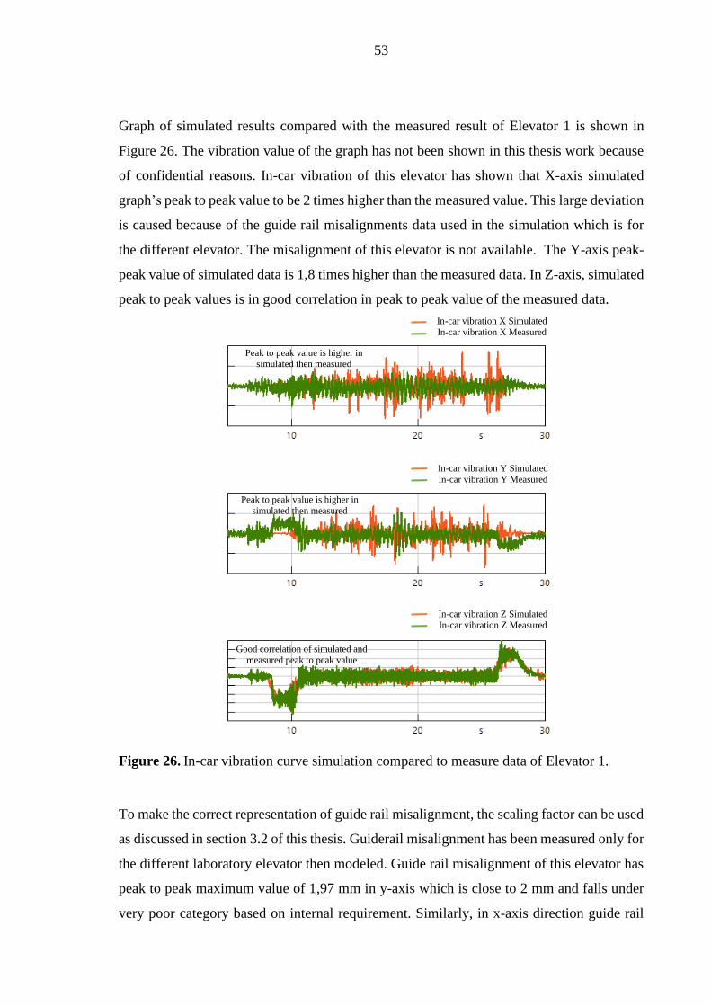
53
Graph of simulated results compared with the measured result of Elevator 1 is shown in
Figure 26. The vibration value of the graph has not been shown in this thesis work because
of confidential reasons. In-car vibration of this elevator has shown that X-axis simulated
graph’s peak to peak value to be 2 times higher than the measured value. This large deviation
is caused because of the guide rail misalignments data used in the simulation which is for
the different elevator. The misalignment of this elevator is not available. The Y-axis peak-
peak value of simulated data is 1,8 times higher than the measured data. In Z-axis, simulated
peak to peak values is in good correlation in peak to peak value of the measured data.
Figure 26. In-car vibration curve simulation compared to measure data of Elevator 1.
To make the correct representation of guide rail misalignment, the scaling factor can be used
as discussed in section 3.2 of this thesis. Guiderail misalignment has been measured only for
the different laboratory elevator then modeled. Guide rail misalignment of this elevator has
peak to peak maximum value of 1,97 mm in y-axis which is close to 2 mm and falls under
very poor category based on internal requirement. Similarly, in x-axis direction guide rail
Peak to peak value is higher in
simulated then measured
Peak to peak value is higher in
simulated then measured
Good correlation of simulated and
measured peak to peak value
In-car vibration X Simulated
In-car vibration X Measured
In-car vibration Y Simulated
In-car vibration Y Measured
In-car vibration Z Simulated
In-car vibration Z Measured

54
misalignment has peak to peak maximum value of 1.46 mm which is close to 1.5 mm and
falls under the poor category based on the internal requirement. The assumption is, that
modeled elevator has more accurately installed guide rails. Therefore, to represent more
accurate installed guide rails, an average of right and left guide rail misalignments were
considered and scaled down with a factor of 0.4 (in average right and left guide rail) which
resulted in peak to peak value of 0.7 mm in y-axis direction and x-axis direction, the reducing
factor used was 0.7 (in average for right and left guide rail) which resulted in peak to peak
value of 0.75mm. After scaling down of misalignments the elevator model has shown a good
graph fit with the measured graph as can be seen in Figure 27.
Figure 27. In-car vibration curve simulation compared to measure data of Elevator 1 after
correct representation of guide rial misalignment.
Elevator 2 is validated with measured data as seen in Figure 28. The data measured is for the
elevator with sliding shoes but with a different experimental motor than the one used in the
simulation model. Here also guide rail misalignment scale factor of 0.4 in y-axis direction
and 0.7 BFT direction of measure elevator has been used. The sliding guide shoes is modeled
In-car vibration X Simulated
In-car vibration X Measured
In-car vibration Y Simulated In-car vibration Y Measured
In-car vibration Z Simulated
In-car vibration Z Measured
Good correlation of simulated and
measured peak to peak value for all
direction of vibration

55
by changing stiffness in y-axis and x-axis direction and friction coefficient of 0.2 as
discussed in section 3.2.1. High correlation in all three directions vibration can be seen.
Figure 28. Elevator 2 simulated vibration vs measured vibration.
The modeling of the elevator rated load 480 Kg model has been done with its specifications.
The guide rail misalignment has been used same as of model elevator rated load 630 Kg.
Due to the unavailability of the measured data for this elevator, validation was not possible.
However, this model was assumed to be model accurately as elevator rated load 630 Kg and
elevator rated load 480 Kg comes from the same elevator platform and has only differences
in the geometrical, mass and inertia specification. The elevator rated load 630 Kg and
elevator rated load 480 Kg were both modeled using the same technique with the same
stiffness and damper for the majority of the components.
In-car vibration X Simulated
In-car vibration X Measured
In-car vibration Y Simulated In-car vibration Y Measured
In-car vibration Z Simulated
In-car vibration Z Measured
Good correlation of simulated and
measured peak to peak value for all
direction of vibration

56
4.1.2 Frequency domain validation
The peak to peak validation has shown good results in the last chapter, however, it is
important to validate the model on the frequency domain. The frequency domain validation
will provide the model to gain more reliability. From frequency domain validation, it is
possible to find out at what frequencies the system is vibrating and help to find what is the
root cause of these frequencies. The Frequency domain validation of Elevator 1 and Elevator
2 has been done. Figure 29 shows the Fast Fourier transform (FFT) graphs of the measured
and simulated signal where the roller guide shoes have been used. The vertical vibration of
the elevator is only discussed in the frequency domain as vertical vibrations provide
information on the status of several components, such as guide shoe wear, incorrect motor
bedplate design, and improper guide rails installation, and so on along with the opportunity
to develop ride comfort.
Figure 29. FFT of Elevator 1 of measured and simulated data.
In the above figure, the FFT graphs have shown similar resonances taking place at similar
frequencies on both measures and simulated signals. The supply frequencies at 37.45 Hz and
its second harmonics at 74 Hz, the motor speed at 1.87 Hz, traction sheave eccentricity at
4.45 Hz, slot frequency at 67.4 Hz are seen in both measured signal and simulated signals.
These are fundamental frequencies of motor which are traveling from motor via rope to
pulley beam to car. In the simulated signal the supply frequency is not seen, however, the
eigenfrequency of the motor mounting has been seen at 24 Hz. This motor mounting
eigenfrequencies had been also seen in the FEM calculation eigenfrequencies for modes for

57
the same motor as discussed in section 3.2. During the frequency response analysis (see
section 3.2.2), the floor mode at 107 Hz is found for this elevator which has been tuned in
the model. However, this floor mode is not visible in the FFT since the graph plotting is only
fitted to 100 Hz because the measurement data is only credible up to that frequency.
The FFT graph for the measured and simulated signal of Elevator 2 is present in Figure 30.
The fundamental motor frequencies are clearly seen in both the graphs; however, the
measured signal has also shown excitation at the frequency 94 Hz can be seen in a blue
square box in Figure 30, which is not motor excitation. As discussed in section 3.2.2, the
frequency response analysis of the elevator with sliding guide shoes shows the floor mode
at 92 Hz for this elevator therefore, it is concluded that this frequency could be coming from
the floor resonance. In the result, the floor eigenfrequency is seen in the simulated signal in
a similar frequency range to the measured signal.
Figure 30. FFT of Elevator 2 of measured and simulated data.
4.1.3 Comparison of roller and sliding guide shoes
The difference between roller guide shoe and sliding guide shoes modeling is the stiffness
value, friction coefficient value and floor eigenfrequencies as shown in Table 4. The elevator
car floor eigenfrequency is dependent on the stiffness value of guide shoes therefore
difference in stiffness value of roller and sliding guide has led to the difference in the floor
eigenfrequencies. The roller guide has roller assembly consists of three separate identical
rollers. Each of the rollers is fixed to the guide roller frame with damper isolation pads. The

58
all rollers in the roller guide have an initial compression of 1 mm against the guide rail in
reality which is not used in the SimulationX model. The sliding guide shoe consists of a u-
shaped plastic sliding insert, 2-part sheet metal frame and a rubber isolator and has a
clearance of x-axis direction of 1mm which again is not used in the SimulationX model.
Table 4: Different between roller and sliding guide shoes model
Roller guide shoes Sliding guide shoes
• Stiffness of 250 N/mm in both y-
axis and x-axis direction
• The friction coefficient of roller
assembly is 0.05
• Floor eigenfrequency for Elevator 1
is 87 Hz and in Elevator 3 is 94 Hz
• Stiffness of 175 N/mm in y-axis and
325N/mm x-axis direction
• The friction coefficient of sliding
assembly is 0.2
• Floor eigenfrequency for Elevator 2
is 96 Hz and in Elevator 4 is 81 Hz
Comparison Elevator 1 and Elevator 2 has been carried out to understand its impact in the
lateral and vertical vibration and as well all in frequency domain seen in Figure 31. In X-
direction, the higher stiffness value of sliding guide shoes (325 N/mm in x-axis), has higher
vibration amplitude in time domain result and in frequency domain result, slight shift toward
higher frequency can be seen in the FFT graph. Similarly, in Y-direction, lower stiffness
value of sliding guide shoes (175 N/mm in y-axis), lower vibration amplitude and slight shift
toward lower frequency can be seen in FFT. In Z-direction, less vibration can be seen in
sliding guide shoes as the floor eigenfrequency is tuned to be 94 Hz, which requires higher
rotational stiffness than of 87 Hz (roller guide shoes). A higher stiffness value has lower
vibration. The effect of the difference of guide shoes stiffness value can be also seen in the
forces of guide shoes.

59
Figure 31. Time and frequency domain vibrations of roller guide shoe and sliding guide
shoes.
The torque produced by the motor changes as the friction coefficient increases from 0.05 to
0.2 When the power loss caused by friction in the guide shoes is greater, the needed motor
torque is increased to keep the elevator cars moving smoothly. This creates a fluctuation in
motor torque generation as can be seen in sliding guide shoes in Figure 32. This finding can
be used to diagnose a lubrication deficiency that generated a high friction coefficient
between the guide rail and guide shoes.

60
Figure 32. Motor toque and power loss of roller guide shoe and sliding guide shoes.
4.1.4 Validation analysis
The time and frequency domain validation comparison with two different elevators was
successful as the simulated results correlated well with the laboratory measured quantities
of elevators. In time domain vibration validation, maximum peak to peak values at nominal
speed were the main criteria for the validation. The time domain validation demonstrates not
only a correlation in the peak to peak value at the nominal run but also a well-fitted vertical
vibration at the time of acceleration and deceleration period. However, there were some
minor deviations between the simulation and measured data of the position and velocity of
the car at acceleration and deceleration mainly caused by the difference in car movement
time, jerk value and inertia between simulated and measured data. The shift in the vibration
phase is observed in measured data during acceleration and deceleration in the y-axis
vibration, which is produced by measurement error and is not seen in simulated results.
Validation comparisons also reveal many differences in the shape and amplitude of
measured data and simulation data curves. Factors contributing to these discrepancies
include characteristics differences between actual elevators and their simulated counterparts,
such as stiffness and damper coefficient of different components, and guide rails
misalignment. These differences might also explain why some excitation frequencies are not
visible in the simulated FFT when compared to the observed FFT.
Motor torque
Power loss

61
4.2 Sensitivity analysis
To verify and get reliable the model, a sensitivity analysis is performed by altering several
parameters. Elevator 1, Elevator 2, Elevator 3, and Elevator 4 are used for sensitivity
analysis. The parameters chosen for these analyses are nominal run parameters such as load,
no. of rope, traveling cable linear density, compensation chain linter density, travel height,
speed, acceleration, and balancing ratio of counterweight. During each simulation run, only
one parameter is changed, and the rest are kept with the default parameter. The purposes of
this study are to observe model sensitivity and as well as to generate synthetic data for
malfunction identification.
The default parameter of the simulation run all model
• Run type: - Down run from (top to 1st floor)
• Travel height 18 m (+1.1 m pit) from Elevator 1
• Travel height 13.26 m (+1.05 m pit) from Elevator 3
• In-car load 80 Kg
• Acceleration 0.5 m/s^2
• Rope number – 4
• Speed 1 m/s
• Nominal Jerk: 0.64 m/s³
• Traveling cable liner density 0.435 Kg/m
• No compensation chains
• Motor
A total of 72 variants run are simulated and peak to peak value of lateral and vertical
vibration for up run and down run. The combination of variants is presented in Table 5. As
a result of the sensitivity study, it was discovered that white noise causes random deviations
discussed in section 4.5, and hence white noise was not set as constant during sensitivity
analysis. The lateral vibration and vertical vibration for all the simulation runs are analyses
for the down run only. For a better comparison of the four model’s peak to peak value of
vibration, the bar chart is used.
To find maximum the peak to peak value from the vibrations result in the time domain is a
time-consuming process and most like to make a mistake. The python script was developed

62
to circumvent these issues. The simulation data was entered into Python, and the script
determined the highest peak to peak value as well as the precise time when the peak to peak
occurred.
Table 5: Variants combination
4.2.1 Load case
During elevator system operation, the in-car load i.e. the number of passengers often
fluctuates. Because of the variable elevator load, the vibration behavior is predicted to
change. The changes in eigenfrequency and decrease in car oscillation amplitude are
expected when increasing the load in the all elevator model. The peak to peak value for all
four models is presented in Figure 33. (Herrera et al. 2014, p. 125.)

63
Figure 33. Load impact in peak to peak value of in-car vibration.
The Elevator 1 and 3 models has responded as predicted, with a drop in the peak to peak
value in all three directions of vibration as shown in Figure 33. Similar lateral vibration
responses can be found for both models with sliding guide shoes, however, the vertical
vibration amplitude is the smallest when the load is 315 kg. When the load in the car is half
of the rated load, the elevator car to counterweight balancing ratio is approximately 50%,
and the motor torque necessary to carry out the operation is at its lowest. Less motor torque
is generated, which results in less vibration being produced and transferred to the vehicle via
the suspension rope. Vibration reduction can be seen in Figure 34 of Elevator 2.
Figure 34. Vibration and frequency domain at different load cases.
0
10
20
30
40
50
X Y Z X Y Z X Y Z X Y Z
Elevator 1 Elevator 2 Elevator 3 Elevator 4
Gal
Load Case
Incar load 80Kg Incar load 315Kg Incar laod 630Kg
FFT

64
4.2.2 Rope case
When the number of suspension ropes increases, the tension on each rope is decreased
making the system more flexible. Due to the flexible hoisting system, rope oscillation is
decreased, and less vibration is transmitted to the car, causing less vibration in-car. Figure
35 depicts the effect of changing the number of ropes on car vibration. The number of ropes
is varying from 4, 5 and 6 for all four-elevator models. The peak to peak values are
fluctuating and no clear trend can be seen, however lateral and vertical vibration peak to
peak values are close to each other. It could be explained as the model has randomness shown
in subsection 4.2.9 therefore it is challenging to draw a clear conclusion from this study.
Overall, less vibration can be seen while increasing the rope number from 4 to 6. However,
no significant change in the peak-to-peak value.
Figure 35. Number of rope impact in peak to peak value of in-car vibration.
The number of suspension rope impacts are investigated without any randomness in the
model, by using the same white noise for all simulation runs. For this investigation, Elevator
3 was employed, and all three rope variations (4,5,6) were used. When the number of ropes
is increased, the peak to peak value of both lateral and vertical vibration is found to decrease.
However, this shift in the peak to peak value of lateral vibration occurs within 1 gal of
vibration, but vertical vibration has a vibration drop of almost 10 gals. The model has
responded as expected when the randomness was eliminated.
0
5
10
15
20
25
30
35
40
45
X Y Z X Y Z X Y Z X Y Z
Elevator 1 Elevator 2 Elevator 3 Elevator 4
Gal
Rope Case
Rope 4 Rope 5 Rope 6

65
4.2.3 Speed case
For speed variations between 0.63 m/s to 1.75 m/s, the same motor but of different versions
are used. For speed 0.63m/s and 1m/s motor_V1 has been used and for speed 1.6 m/s and
1.75 m/s motor_V2 has been used for the simulation. The masses and inertia of tensor of
rotation component and mounting translation and rotational stiffness were kept constant for
both motor versions.
The speed of an elevator has a significant influence on the quality of the ride i.e. vibration.
The effect of guide shoes and misalignment of the guide rails is amplified as travel speed
increases (Lemiao et al. 2020, p. 6). As a result, at lower speeds, the vibration amplitude
should be smaller, while at higher speeds, it should be larger. When the speed is reduced
from 1m/s to 0.63 m/s, the lateral vibration is reduced by more than 50 %, as shown in Figure
36. When the speed is raised from 1 m/s to 1.75 m/s, the lateral vibration has risen by about
250%. When it comes to lateral vibration, all four models behave well. Figure 36 illustrate
that the vertical vibrations for all model are changing from each other. The vertical vibration
Peak to peak value has no clear trend and it is challenging to conclude it. This could also be
because of randomness present in the model.
Figure 36. Speed impact in peak to peak value of in-car vibration.
To examine the influence of speed changes in the lateral direction in full depth, the Elevator
3 model has been used. This study discusses how the guide rail's misalignment impact is
0
10
20
30
40
50
60
X Y Z X Y Z X Y Z X Y Z
Elevator 1 Elevator 2 Elevator 3 Elevator 4
Gal
Speed Case
Speed 0,63 m/s Speed 1 m/s Speed 1,6 m/s Speed 1,75 m/s

66
exacerbated when speed increases from 1m/s to 1,75 m/s, as well as its reaction to vibration.
Figure 37 depicts a right rail misalignment (right up), with higher two peaks at 3,1 m and
10,19 m height which is contributing to the highest vibration in the Y direction for both
speed profiles. Higher speed causes a greater shift in the displacement and forces on the
guide shoes, resulting in increased vibration throughout the car. The Peak to peak value at
speed 1,75 m/s is 2.5 times higher than of at speed 1 m/s. Figure 37 at the right bottom shows
this effect in guide shoes.
Figure 37. Speed impact to guide shoes forces and to the lateral vibration.
In the model, the supply frequency and slot frequency are proportional to the speed to make
the model parametric. Reducing the speed lowers the supply frequency and slot frequency,
and vice versa. The FFT graph of car vertical vibration Figure 38 clearly shows these
variations in slot and supply frequency. In the lateral direction, one can observe that the
lower speed has a smaller frequency amplitude than the higher speed in the FFT.
Amplification of guide rail misalignment
as travel speed increases
Zoom
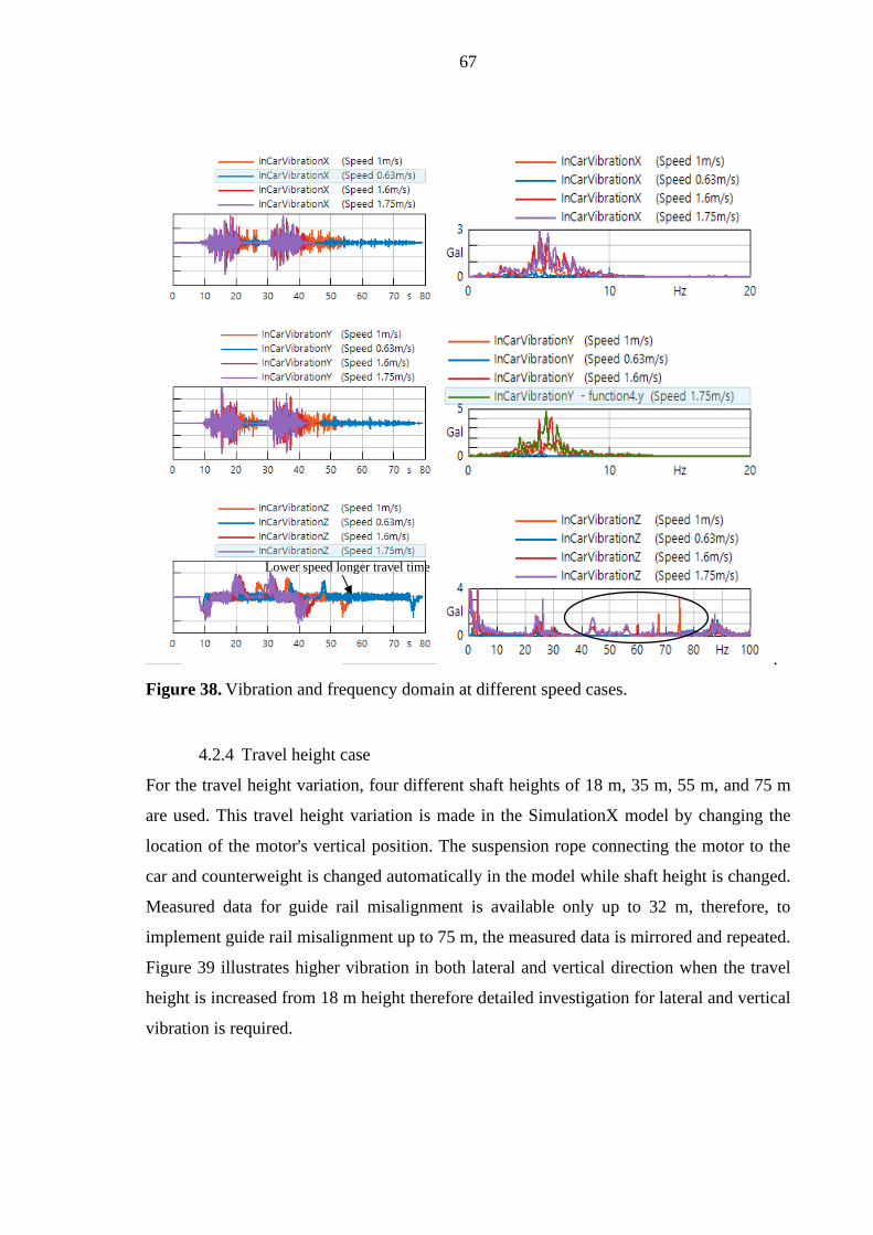
67
.
Figure 38. Vibration and frequency domain at different speed cases.
4.2.4 Travel height case
For the travel height variation, four different shaft heights of 18 m, 35 m, 55 m, and 75 m
are used. This travel height variation is made in the SimulationX model by changing the
location of the motor's vertical position. The suspension rope connecting the motor to the
car and counterweight is changed automatically in the model while shaft height is changed.
Measured data for guide rail misalignment is available only up to 32 m, therefore, to
implement guide rail misalignment up to 75 m, the measured data is mirrored and repeated.
Figure 39 illustrates higher vibration in both lateral and vertical direction when the travel
height is increased from 18 m height therefore detailed investigation for lateral and vertical
vibration is required.
Lower speed longer travel time

68
Figure 39. Travel height impact in peak to peak value of in-car vibration.
The Elevator 1 was used to investigate the impact of changes in travel height in the lateral
and vertical directions in detail. This model's travel height is set at 55 m. When investigating
the guide rail misalignment further, it is discovered that there are peaks with greater
amplitude beyond 20 m. This is explained by the fact that as the height of the guide rial shaft
increases, so does the number of guide rail segment slices, resulting in a greater
misalignment in the structure. Manufacturing error (if the guide rails are not manufactured
straight) and assembly error also known as human error (brackets are used to rigidly fix
guide rail to the building walls and fishplate are used to guide rials to each other) are the
most common causes of guide rail misalignment. As a result, larger guide rail misalignments
can occur after the 18 m height, contributing to a higher peak-to-peak value on the lateral
vibration. This is visible in all models with a travel height greater than 18 m. The highest
peak to peak value in the X-direction is at time 41,8 m, and a bigger misalignment in the
right rail can be observed at time 44,3 m, which demonstrates that when top guide shoes
(vertical distance between guide shoes 2,5 m from top to bottom guide shoes) pass over this
misalignment, a peak is created, as shown in Figure 40. There is also regular excitation after
every 2.5 m of travel after 20 m of shaft height. This is excitation caused by misalignment
at guide rail slices. The length of one guide rail segment is 5 m, and the distance between
guide shoes is about 2.5 m, resulting in contact of a guide shoe to a guide rail edge every 2.5
m, lead to greater vibrations every 2.5 m. Similarly, the larger the misalignment in the Y-
direction, the higher the vibration.
0
10
20
30
40
50
60
70
X Y Z X Y Z X Y Z X Y Z
Elevator 1 Elevator 2 Elevator 3 Elevator 4
Gal
Travel height Case
Travel 18m Travel 35m Travel 55m Travel 75m

69
Figure 40. Impact of travel height of 55 m on guide rail misalignments on lateral vibrations.
The guide rail misalignment has an impact on the vertical vibration as well as can be seen
from the graph in Figure 41. Sharper the spikes in the guide rail misalignment, the higher
the peak-to-peak value can be found in vertical vibration. Sharper spikes in the guide rail
misalignment act as the source of excitation in the model for vertical vibration. This effect
of misalignment is seen in the vertical vibration because of the squeezing effect of the guide
shoes on the flexible floor. The squeezing effect here means when the guide shoes are
passing through higher misalignments (higher guide shoes forces), the flexible floor panels
can bend (up or down) creating space for guide shoes to displace toward each other. This
phenomenon is taking place because the guide shoes are rigidly connected to the floor panels
and floor panels are modeled as flexible and are stiffened by translation and rotation stiffness
values. Further development of the model is going on to avoid the displacement of guide
Steeper the guide rails misalignment,
higher the peak to peak value of
vibration

70
shoes. Higher vibration can be seen in Figure 41 when the car is closer to the motor due to
higher transmission of vibration from motor to car when the rope length is at the shortest.
Figure 41. Travel height impact on Vertical vibration.
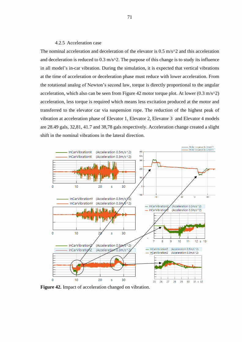
71
4.2.5 Acceleration case
The nominal acceleration and deceleration of the elevator is 0.5 m/s^2 and this acceleration
and deceleration is reduced to 0.3 m/s^2. The purpose of this change is to study its influence
in all model’s in-car vibration. During the simulation, it is expected that vertical vibrations
at the time of acceleration or deceleration phase must reduce with lower acceleration. From
the rotational analog of Newton’s second law, torque is directly proportional to the angular
acceleration, which also can be seen from Figure 42 motor torque plot. At lower (0.3 m/s^2)
acceleration, less torque is required which means less excitation produced at the motor and
transferred to the elevator car via suspension rope. The reduction of the highest peak of
vibration at acceleration phase of Elevator 1, Elevator 2, Elevator 3 and Elevator 4 models
are 28.49 gals, 32,81, 41.7 and 38,78 gals respectively. Acceleration change created a slight
shift in the nominal vibrations in the lateral direction.
Figure 42. Impact of acceleration changed on vibration.

72
4.2.6 Balancing ratio case
The balancing ratio implies the total load on the car side of traction sheave to the total load
on the counterweight side. The motor application is reduced when the balancing ratio is close
to 50%. In this situation, the work done required for completing the down run or up run by
elevator is minimum, hence the least motor torque is required. The variation of balancing
ratio had been done by changing the weight of the counterweight in the SimulationX model.
In this study, the balancing ratio of 40% and 50% have been used. 40% is considered to be
the worst balancing ratio while 50% is considered as the best balancing ratio. The car mass
or load has been kept constant in all the cases therefore no significant changes in the lateral
vibration can be seen. However, in the vertical vibration one can see from Figure 43 that at
50% balancing ratio, the peak to peak value has been the least. This is because at 50%
balancing ratio the motor torque production to carry out work is least which leads to less
excitation being transferred to the car through suspension rope. This phenomenon also can
be seen in the load case variate simulation for elevator model with sliding guide shoes, where
at load 360 kg the vertical vibration is registered to be least.
.
Figure 43. Balancing ratio impact in peak to peak value of in-car vibration.
4.2.7 Traveling cable case
The weight of the moving cable is attached to the bottom of the elevator car. When the
elevator travels from the lowest level to the top floor, the weight of the traveling cable
increases, and it reduces on the down run. Depending on where it is attached and the linear
density of the cable, it might cause a dynamic imbalance in the car which has an influence
on ride comfort. For all four simulation models, the linear density of the cable ranges from
0
10
20
30
40
50
X Y Z X Y Z X Y Z X Y Z
Elevator 1 Elevator 2 Elevator 3 Elevator 4
Gal
Balancing % Case
Balancing 40% Balancing 50 %

73
0.435 kg/m to 1,842 kg/m. According to the results shown in Figure 44, traveling cable linear
density has little influence on lateral vibration, and in vertical vibration, the vibration
amplitude is lowest when the traveling cable linear density is 0.908 kg/m. This is suspected
to be happening due to some resonance taking place in the remaining cases.
Figure 44. Travelling cable impact in peak to peak value of in-car vibration.
4.2.8 Compensation chain linear density case
The compensation chain, like the traveling cable, is linked to the bottom of the elevator car
and also the counterweight. The overall weight of the car progressively grows during the
uprun and reduces during the down run, whereas the total weight of the counterweight
changes in the opposite direction. Compensation chains are typically used to provide ease
on the hoisting mechanism when the elevator is operating without any passengers or with
fewer passengers than of the capacity. Normally for the low-rise elevators, there is no
compensation chain used since the travel height are these elevators are low. In this case, two
alternative compensation chains are utilized and simulated with linear densities of 1.5 kg/m
and 3 kg/m using all four models to determine if the model is sensitive compensation chain.
As a result of the increased linear density of the compensating chain, one may expect
increased vibration during up run and decreased vibration during down run. According to
the results given in Figure 45. The linear density of the compensation chain has little impact
on lateral vibration, and there is no apparent pattern in the vertical vibration peak to peak
value. This is caused by the unpredictability that exists in the model.
0
10
20
30
40
50
X Y Z X Y Z X Y Z X Y Z
Elevator 1 Elevator 2 Elevator 3 Elevator 4
Gal
Travelling cable linear density Case
Cable density 0.435kg/m Cable density 0.908kg/m Cable density 1.842kg/m

74
Figure 45. Compensation chain impact in peak to peak value of in-car vibration.
White noise was set as constant to avoid randomness in the model to investigate
compensation chain impact. Elevator 1 was used for this study, and all three variations (0
kg/m, 1.5 kg/m, 3 kg/m) of liner density is used. The results of these simulations are shown
in Figure 46. The peak to peak value of both lateral and vertical vibration has been seen to
be decreasing when the compensation chain linear density has increased. However this
change in the peak to peak value is taking place with 1 gal of vibration, this is because the
change in the total weight after adding or subtracting to the car is only 56,7 kg (with
companion chain linear density 3 kg/m) which is negligible to affect vibration. Nevertheless,
as expected the vibration is reduced. In the graph, it is seen that when the elevation car has
compensation chain weight (starting of simulation run in the green box) the vibration in all
directions is less than when the elevator car has no compensation chain weight (end of
simulation run in red box).
0
10
20
30
40
50
X Y Z X Y Z X Y Z X Y Z
Elevator 1 Elevator 2 Elevator 3 Elevator 4
Gal
Compensation chain linear density Case
No compensation chain Chain density 1.5kg/m Chain density 3kg/m

75
Figure 46. Compensation chain impact in-car vibration of Elevator 1.
4.2.9 Study of assumptions in the model
Sensitivity studies of different nominal run cases revealed that the model had a modest
quantity of randomness. To study the root causes of this randomness in the model, Elevator
3 model is used. Three consecutive simulations were performed without making any changes
in the model and the results indicated a 3 gals, 2 gals, and 4 gals fluctuation in Peak to peak
values of X, Y and Z direction vibrations respectively. The model contains white noise to
provide additional generic excitation to motor and car. The implementation of generic
excitation in the model to account for possible excitation sources such as friction and other
noise. To understand the impact of white noise on the vibration, three consecutive
simulations were performed without white noise in the model. The results of these
Higher vibration when
compensation chain linear
density is 3 kg/m
Nearly no change in vibration when compensation chain
linear density is 3 kg/m
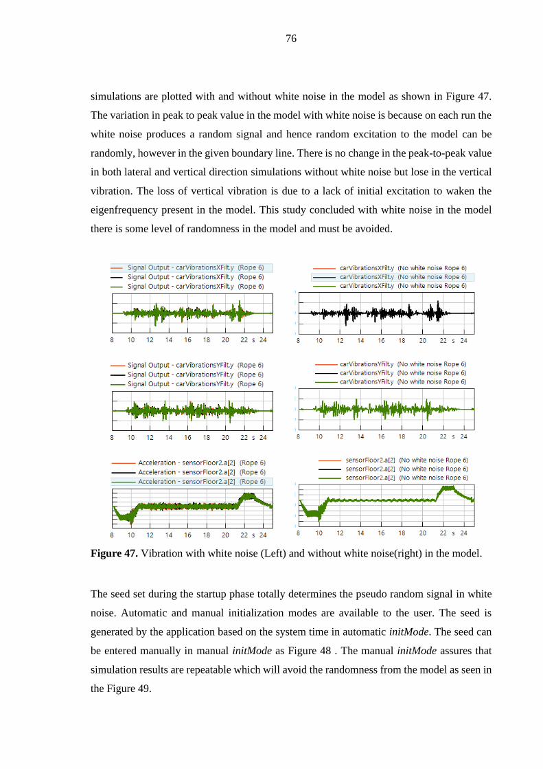
76
simulations are plotted with and without white noise in the model as shown in Figure 47.
The variation in peak to peak value in the model with white noise is because on each run the
white noise produces a random signal and hence random excitation to the model can be
randomly, however in the given boundary line. There is no change in the peak-to-peak value
in both lateral and vertical direction simulations without white noise but lose in the vertical
vibration. The loss of vertical vibration is due to a lack of initial excitation to waken the
eigenfrequency present in the model. This study concluded with white noise in the model
there is some level of randomness in the model and must be avoided.
Figure 47. Vibration with white noise (Left) and without white noise(right) in the model.
The seed set during the startup phase totally determines the pseudo random signal in white
noise. Automatic and manual initialization modes are available to the user. The seed is
generated by the application based on the system time in automatic initMode. The seed can
be entered manually in manual initMode as Figure 48 . The manual initMode assures that
simulation results are repeatable which will avoid the randomness from the model as seen in
the Figure 49.

77
Figure 48. White noise setting from constant output.
Figure 49. Vibration and frequency domain of constant white noise to motor and car.
The anomalies found in the result were investigated and root causes were found to be either
because of white noise excitation or flexible floor modeling. The white noise excitation
replicates the real model to produce results with small variations. This phenomenon is also
found when multiple measurements are taken for the same real elevator. This is a useful
feature to have in the model, but it is inapplicable for sensitivity analysis when even a small
change in peak to peak value is important.

78
The sensitivity analysis of several configurations at nominal run confirmed that the model is
sensitive and robust. In the majority of situations, the model behavior was found to be as
projected. There were clear patterns in the dynamic response of the model as well as in the
peak to peak value of vibration. However, the amount of change in peak to peak values found
in the real model under these configurations needs to be validated with measured data
4.3 Load case results and analysis
In the chapter, the results of sag and bounce, car buffer crash and counterweight buffer crash
situation are presented and analyzed.
4.3.1 Sag and bounce
The Elevator 1 model has been used for sag and bouncing phenomena. The sag model is
validated with measured data. During the simulation and measurement of sag and bouncing,
the load used is 89 kg. The car sag is measured by finding the position of the car in relation
to the landing door positioning before and after loading. A 3-dimensional DC accelerometer
is used to measure car bounce. The loading time is set to be at 5 seconds and the loading off
time is at 15 seconds. The sag found in the measurement is less than 2.4 mm and, in the
model, it is found to be 2.24 mm. The comparison of simulated and measured graphs of
bouncing acceleration is represented in Figure 50. The simulated result of car bouncing is
well-fitting with the measured curve and its peak to peak value is 99.25 gals and simulated
is 97.34 gals. For this validation of bouncing vibration, the axial stiffness is multiplied by
0.6 to represent the non-linearity of rope at the lowest floor. The saturation time used is 0.2
seconds. The slight difference at the starting of the curve comes due to differences in the
saturation time used in the model and in real-time. This parameter is challenging to capture
as it happened in a fraction of time. The difference at the end of the curve comes from the
difference in the damper parameter used in the model, which again it challenging to know
the exact value.

79
Figure 50. Sag and bouncing of the elevator (up) and vibration at bouncing (down).
4.3.2 Car buffer run
Elevator 1 has been utilized for car buffer run study and the simulation run has been started
from the third floor to the buffer run. Figure 51 represents the result of the vertical velocity
of the car, counterweight and angular velocity of traction sheave at buffer run. The collision
between the car and buffer has taken place at 15.54 seconds. The velocity of the car after the
collision has come to zero but at 15.90 seconds, it has started to rise and reached 0.7 m/s. At
the same time, the velocity of the counterweight is -0.7 m/s and the angular velocity of the
traction sheave is 7.2 rad/s. From this phenomenon, it can be concluded that when the car is
striking against buffer, the impact of collision leads to bouncing of counterweight. And
because the counterweight is 210 kg more than car weight, it pulls the car upward. Due to a
lack of braking torque, the traction sheave is not stopped after brake activation, allowing this
scenario to occur. Therefore, the brake torque value is reviewed and found out that the motor
is equipped with two brake pads hence twice the brake torque value (2*350 Nm) must be
used in the SimulationX model. The vertical velocity result with a new brake torque value
represents the reality much more, however, there is still a small effect of counterweight as
presented in Figure 51 on the right side.
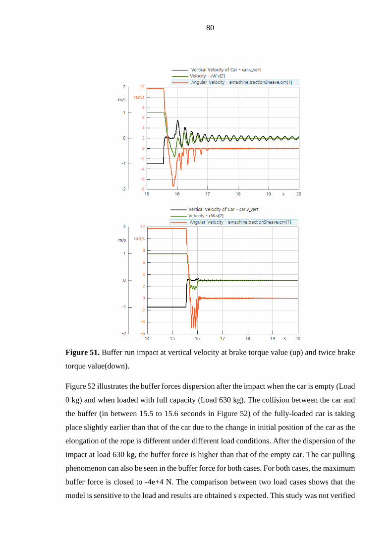
80
Figure 51. Buffer run impact at vertical velocity at brake torque value (up) and twice brake
torque value(down).
Figure 52 illustrates the buffer forces dispersion after the impact when the car is empty (Load
0 kg) and when loaded with full capacity (Load 630 kg). The collision between the car and
the buffer (in between 15.5 to 15.6 seconds in Figure 52) of the fully-loaded car is taking
place slightly earlier than that of the car due to the change in initial position of the car as the
elongation of the rope is different under different load conditions. After the dispersion of the
impact at load 630 kg, the buffer force is higher than that of the empty car. The car pulling
phenomenon can also be seen in the buffer force for both cases. For both cases, the maximum
buffer force is closed to -4e+4 N. The comparison between two load cases shows that the
model is sensitive to the load and results are obtained s expected. This study was not verified

81
since the measured data from the real buffer was unbillable; thus, validation is necessary for
better understanding and a more reliable model.
Figure 52. Buffer force at load 0 kg and 630 kg.
4.3.3 Counterweight buffer run
Elevator 1 has been utilized for the counterweight buffer run and the simulation run has been
started from the sixth floor to the counterweight buffer run. Figure 53 represents the result
of the vertical velocity, buffer force of counterweight at buffer run8 at 0 kg and 630 kg load
case. No significant difference other than the change in the time of buffer impact can be seen
in the curves and this is due to no change in the load of the counterweight. This study was
not validated since the measured data from the real buffer was unbillable; thus, validation is
necessary for better understanding and obtaining a more accurate model.
Figure 53. Velocity and buffer force of counterweight at 0 kg and 630 kg in-car load.

82
4.4 Analysis and discussion
In this thesis, the elevator system is modeled based on a preexisting elevator model and
validated from the laboratory data for position, velocity and vibrations of the elevator car.
During the validation, not only the measured and simulated curves are shown to have a high
correlation, but the model's inability to turn the floor eigenfrequency lower than 81 HZ was
discovered and resolved. In the same way, in the sensitivity analysis, not only the model's
sensitivity and robustness were validated, but also a model with randomness and a significant
effect of squeezing of guide shoes was discovered. Finally, load scenarios were successfully
modeled and assessed. The objectives of this thesis were fulfilled effectively, and numerous
obstacles were encountered and solved along the way, increasing the reliability of the model
predicting the dynamic behavior of elevator systems.
The most critical components, with their parameters contributing to the researched
phenomena, are required to be modeled for an accurate representation of the system.
However, the level of detail required in the model is entirely dependent on the type and
accuracy of the outcomes expected. The most significant components in an elevator system
are the motor, motor mount, rope, guide rails, guide shoes, car mount, pulley beam, elevator
car, and counterweight. The collective effect of each component and its parameters results
in car vibration. The level of detail modeling required for each component for studying their
response in-car vibration is presented in section 3.2. The initial excitations are also crucial
to include in the model since they can cause subsequent resonances to occur. Similarly, a
flexible car model is required for capturing the influence of local mode and its potential
resonances. This provides the answer to the first research question of the thesis.
When the elevator family changes, the parameters of components change as well. The input
parameters provided in Table 2 in Chapter 3 must be updated as per new elevator
specifications that represent a specific elevator. The inputs can be categories into 4 main
parameters i.e. geomaterial information, mass properties, stiffness and damping of
components. These parameters have a high influence on vibration. Thus, these are the most
important parameters to update while changing from one elevator family to another elevator
family and maintaining the accuracy of the results. This is the solution to the thesis's second
research question.

83
While discussing the third research question, to model any load case or malfunction in the
model, the phenomena happening in the real situation must be identified and requirements
to represent the phenomena must be known before replicating in the virtual model. As in sag
and bounce modeling, it was understood that the in-car load is added in a fraction of a second
and its result is measured in the displacement of car position after loading and unloading and
vertical vibration while unloading.
As explained in chapter 2.1.2 for prescriptive maintenance a larger set of data (real or
synthetic data) are required. Synthetic data can carry all kinds of information about the model
along with malfunctions information which can be implemented in the simulation model.
These data are used for creating algorithms from machine learning. With the high-quality
synthetic data availability, artificial intelligence is used for failure signatures recognition and
maintenance indications. During training a prescriptive maintenance algorithm, industry
higher-level information can be provided to detected possible upcoming malfunction and
suggesting possible ways to solve it. In short, the synthetic data provide the raw material for
deep machine learning and artificial intelligence to create signature failure patterns which
are then used in the prescriptive maintenance.

84
5 CONCLUSION AND FUTURE WORK
The main aim of this thesis was to model, validate and perform sensitivity analysis of the
elevator at the system level in the SimulationX software. For this purpose, four elevators
were modeled with their components and characteristics. The preexisting physics-based
simulation model based on the KONE elevator system was utilized as a reference model.
The elevator model of Elevator 1 and Elevator 2 were successfully validated with respective
measured data based on peak to peak values of the lateral and vertical vibrations. Validation
comparisons show several discrepancies between test data and simulation data curves in
terms of their form and amplitude. The major cause is the discrepancies in characteristics
between the real and simulated elevators, such as stiffness and damper values of different
components, as well as guide rail misalignments. During the comparison of the influence of
rolling and sliding guide shoes on vibration, it was discovered that increasing the stiffness
value of guide shoes resulted in an increase in peak to peak value and vice versa. The friction
coefficient value between the guide rail and the guide shoes demonstrates the relationship
between power loss at guide shoes and motor torque requirement.
The sensitivity analysis of the model provided important findings which could be further
utilized to develop the elevator model. Higher spikes in the guide rail misalignment have a
significant influence on the vertical vibration peak to peak value due to the squeezing effect
of the guide shoes on the flexible floor however, in reality, there is a squeezing effect but
much smaller and hardly its effect is seen in the vertical vibration. Thus, in the future, the
model requires further modification to limit the effect of this phenomenon. In addition,
sensitivity analysis also shows that the model also includes a modest level of randomness.
The randomness in the model caused the inconsistency of multiple configurations study
results. The utilization of white noise excitation in the car and motor was identified to be the
fundamental cause of this randomness. For each simulation, the white noise was configured
to generate random signals thus causing random excitation. However, randomness can be
avoided by configuring the white noise to generate a constant signal. Overall, the simulation
model demonstrated its sensitivity and robustness in projecting the dynamic behavior of
elevator systems in nominal scenarios.

85
The three most common load case scenarios of an elevator - sag and bounce, car buffer run,
and counterweight buffer run were simulated and analyzed. The sag and bounce were
validated with the measured data and the comparison between simulation results to test
results showed a good correlation. These load case modeling demonstrated the possibility to
model and analyze several other types of load cases or malfunctions which further can be
simulated with several configurations to understand the case behavior with changing
configurations.
In the future, Elevator 3 and Elevator 4 can be validated with measured data from that
specific real elevator. The specific measured guide rails misalignment of the model elevator
rated load 630 kg and elevator rated load 480 kg can be utilized in the model and compare
with their simulated and measured in-car vibration data to validate the model. The roller
guide shoes model containing pretension and end stopper, while sliding guide shoes having
a clearance in the y-axis direction can be used in the model to represent maximum
functionalities of real guide shoes. The nonlinear stiffness value of sliding guide shoes can
also be introduced in the model. The guide rail can be modeled to be flexible. This
advancement in the model will enable it to capture almost all dynamic behavior while also
increasing its sensitivity and robustness.
Several other parameter configurations can be simulation at nominal scenario. Many elevator
malfunctions such as flat roller of guide shoes, incorrect installation of guide rails, lack of
lubricant oil causing high friction between roller guide shoes and rails for sliding guide
shoes, tilting of the car due to load imbalance and many more, can be modeled, their impact
in-car vibration can be studied and synthetic data can be generated. The generated synthetic
data from these nominal run configurations and malfunctions can be validated from real data
when possible and then can be used for machine learning and artificial intelligence to find
signature patterners in the time domain or the frequency domain. Prescriptive maintenance
can be established using a combination of data captured by sensors and data generated from
physics-based simulation to not only anticipate failure but also provide recommendations on
how to effectively resolve the problem.

86
REFERENCES
Amirouche, F. 2006. [Chapter 5:] Rigid-Body Kinematics. In: Fundamentals of Multibody
Dynamics: Theory and Applications. Birkhäuser Boston, Pp. 41-55.
Aspentech. 2021. Prescriptive Maintenance. [Aspentech webpage]. (Updated date
unknown). [Referred 19.8.2021]. Available: https://www.aspentech.com/en/apm-
resources/prescriptive-maintenance
Baharudin, M. E. 2016. Real-time simulation of multibody systems with applications for
working mobile vehicles. Lappeenranta University of Technology, Pp. 41-43.
Baobing, W. & Baras, J. S. 2013. HybridSim: A Modeling and Co-simulation Toolchain for
Cyber-Physical Systems. IEEE/ACM 17th International Symposium on Distributed
Simulation and Real Time Applications, Pp. 70-75.
Brezina, T., Hadas , Z. & Vetiska, J. 2011. Using of Co-simulation ADAMS-SIMULINK
for Development of Mechatronic Systems. Proceedings of 14th International Conference on
Mechatronics, MECHATRONIKA. Trencianske Teplice, Slovakia. 1-3.6.2011. IEEE. Pp.
59-64.
Centomo, S., Dall’Ora, N. & Fummi, F. 2020. The Design of a Digital-Twin for Predictive
Maintenance. 25th IEEE International Conference on Emerging Technologies and Factory
Automation (ETFA). Vienna, Austria. 8-11.9.2020. Pp. 1781-1788.
Çınar, Z. M., Abdussalam N. A., Zeeshan, Q., Korhan, O., Asmael, M. & Safaei, B. 2020.
Machine Learning in Predictive Maintenance towards Sustainable Smart Manufacturing in
Industry 4.0. Machine Learning and AI Technology for Sustainability, 12: 19. Pp. 8211.

87
Edrmedeso. 2020. Simulation Leadership Forum. [Edrmedeso webpage]. Updated
December 22, 2020. [Referred 1.8.2021]. Available:
https://digitallabs.edrmedeso.com/blog/gkn-vs-liu-vs-gbs-simulation-leadership-forum
Flores, P. 2015. Definition of Multibody System. In: Concepts and Formulations for Spatial
Multibody Dynamics. SpringerBriefs in Applied Sciences and Technology, Pp. 1-63.
Ford, P. J., Amiri, E. & Mendrela, E. 2016. Electric elevator drive with position control.
Electrical Engineering, 98. Pp. 307–319.
Hahsler, M., Bolaos, M. & Forrest, J. 2017. Introduction to stream: An Extensible
Framework for Data Stream Clustering Research with R. Journal of Statistical Software, 76:
14. Pp. 1-45.
Herrera, I., Su, H. & Kaczmarczyk, S. 2014. Influence of the Load Occupancy Ratio on the
Dynamic Response of an Elevator Car System. Applied Mechanics and Materials, 706. Pp.
128-136.
Huang, Q., Li , Z. & Xue, H. 2018. Multi-body dynamics co-simulation of hoisting wire
rope. The Journal of Strain Analysis for Engineering Design, 53: 1. Pp. 36-45.
Ishii, T. 1994. Elevators for skyscrapers. IEEE Spectrum, 31: 9. Pp. 42-46.
Kelvin, M. K. 2007. A simulation study of predictive maintenance policies and how they
impact manufacturing systems. University of Iowa, Pp. 1-2.
Kheir, A. 2015. Tall Buildings and Elevators: A Review of Recent Technological Advances.
Buildings, 5:3. Pp. 1070-1104.
Klein , P. & Bergmann, R. 2018. Data Generation with a Physical Model to Support Machine
Learning Research for Predictive Maintenance [web document]. Trier: 2018 [Referred

88
16.3.2021]. Business Information Systems II University of Trier. Pp. 12. Available in PDF-
file: http://ceur-ws.org/Vol-2191/paper22.pdf
KONE. 2013. [ Slideshare webpage]. (Updated date unknown). [Referred 13.3.2021].
Available: https://www.slideshare.net/suleymanaliyev/general-presentation-ikma24736261
Kovacevic, J. 2017. What is Prescriptive Maintenance? [web document]. Updated 5.6.2017.
[Referred 12.6.2021]. Available: https://hpreliability.com/what-is-prescriptive-
maintenance/
Lemiao, Q., Zili, W. & Shuyou , Z. 2020. A Vibration-Related Design Parameter
Optimization Method for High-Speed Elevator Horizontal Vibration Reduction. Shock and
Vibration, Pp. 1-20.
Liu, Y., Yu, H., Li, G. & Li, Z. 2015. Modeling and Simulation of the drive system of
elevator based on AMESIM. Proceedings of the 3rd International Conference on Material,
Mechanical and Manufacturing Engineering. Guangzhou, China. 27-28.6.2015. Atlantis
Press. Pp. 1120-1124.
Mathworks. 2021. Modeling Joint Connections. [Mathworks webpage]. (Updated date
unknown). [Referred 26.5.2021]. Available: https://se.mathworks.com/help/physmod-
/sm/ug/joints.html
Modelon. 2020. FMI. [Modelon webpage]. (Updated date unknown). [Referred 6.3.2021].
Available: https://www.modelon.com/functional-mock-up-interface-fmi/
Nikravesh, P. E. 2004. An Overview of Several Formulations for Multibody Dynamics.
Springer, Pp. 189-196.
Parrott, A. & Warshaw, L. 2017. Industry 4.0 and the digital twin [web document]. Deloitte:
September 2017 [Referred 26.6.2021]. A Deloitte series on Industry 4.0, digital
manufacturing enterprises, and digital supply networks. Pp. 20. Available in PDF-file:

89
https://www2.deloitte.com/content/dam/Deloitte/kr/Documents/insights/deloittenewsletter-
2017/26_201706/kr_insights_deloitte-newsletter-26_report_02_en.pdf.
SimulationX. 2016. Getting started. [SimulationX webpage]. Updated January 2021.
[Referred 6.2.2021]. Available: http://doc.simulationx.com/4.0/1033/Default.htm#-
Tutorials/GettingStarted.htm
Spiegelhauer , M. & Schlecht, B. 2020. Efficient modelling of flexible cable-pulley systems.
Forsch Ingenieurwes, 85. Pp. 67-75.
Westin, C. 2018. Modelling and Simulation of Marine Cables with Dynamic Winch and
Sheave Contact [web document]. Ottawa: June 2018 [Referred 29.2.2021]. Master’s degree
thesis. Carleton University Ottawa. Pp. 151. Available in PDF-file:
https://carleton.ca/mdl/wp-content/uploads/Westin-Cassidy-MASc-ENG-August-2018.pdf
Yin, C. & Mckay, A. 2018. Introduction to Modeling and Simulation Techniques. The 8th
International Symposium on Computational Intelligence and Industrial Applications.
Tengzhou, Shandong, China. 2-6.9.2018. Pp. 2-4.


![[EN] Aastra - Vertical Market - Transportation](https://img.pdfslide.us/doc/110x75/54b88d154a7959b0668b47b5/en-aastra-vertical-market-transportation.jpg)