Embed Size (px)
Citation preview

University of KentuckyUKnowledge
University of Kentucky Master's Theses Graduate School
2005
SIMULATION OF LOW-RE FLOW OVER AMODIFIED NACA 4415 AIRFOIL WITHOSCILLATING CAMBERVamsidhar KatamUniversity of Kentucky
Click here to let us know how access to this document benefits you.
This Thesis is brought to you for free and open access by the Graduate School at UKnowledge. It has been accepted for inclusion in University ofKentucky Master's Theses by an authorized administrator of UKnowledge. For more information, please contact [email protected].
Recommended CitationKatam, Vamsidhar, "SIMULATION OF LOW-RE FLOW OVER A MODIFIED NACA 4415 AIRFOIL WITH OSCILLATINGCAMBER" (2005). University of Kentucky Master's Theses. 339.https://uknowledge.uky.edu/gradschool_theses/339

ABSTRACT OF THESIS
SIMULATION OF LOW-RE FLOW OVER A MODIFIED NACA 4415 AIRFOIL WITH OSCILLATING CAMBER
Recent interest in Micro Aerial Vehicles (MAVs) and Unmanned Aerial Vehicles (UAVs) have revived research on the performance of airfoils at relatively low Reynolds numbers. A common problem with low Reynolds number flow is that separation is almost inevitable without the application of some means of flow control, but understanding the nature of the separated flow is critical to designing an optimal flow control system. The current research presents results from a joint effort coupling numerical simulation and wind tunnel testing to investigate this flow regime. The primary airfoil for these studies is a modified 4415 with an adaptive actuator mounted internally such that the camber of the airfoil may be changed in a static or oscillatory fashion. A series of simulations are performed in static mode for Reynolds numbers of 25,000 to 100,000 and over a range of angles of attack to predict the characteristics of the flow separation and the coefficients of lift, drag, and moment. Preliminary simulations were performed for dynamic mode and it demonstrates a definitive ability to control separation across the range of Re and AoA. The earlier experimental work showed that separation reduction is gradual until a critical oscillation frequency is reached, after which increases in frequency have little additional impact on the flow. Present numerical simulation results were compared with the previous experiments results which were performed on the airfoil in like flow conditions and these comparisons allow the accuracy of both systems to be determined.
KEYWORDS: Low-Re Flow, Flow Separation, Adaptive Actuator, Flow Control, NACA 4415 Vamsidhar Katam 01/19/2005
Copyright © Vamsidhar Katam 2005

SIMULATION OF LOW-RE FLOW OVER A MODIFIED NACA 4415 AIRFOIL
WITH OSCILLATING CAMBER
By
Vamsidhar Katam
Dr. Raymond P LeBeau
Director of Thesis
Dr. George Huang
Director of Graduate Studies
01/19/2005

RULES FOR THE USE OF THESIS
Unpublished thesis submitted for the Master’s degree and deposited in the University of
Kentucky Library are as a rule open for inspection, but are to be used only with due regard
to the rights of the authors. Bibliographical references may be noted, but quotations or
summaries of parts may be published only with the permission of the author, and with the
usual scholarly acknowledgements.
Extensive copying or publication of the thesis in whole or in part also requires the consent
of the Dean of the Graduate School of the University of Kentucky.

THESIS
Vamsidhar Katam
The Graduate School
University of Kentucky
2005

SIMULATION OF LOW-RE FLOW OVER A MODIFIED NACA 4415 AIRFOIL WITH OSCILLATING CAMBER
THESIS
A thesis submitted in partial fulfillment of the
requirements for the degree of Master of Science in Mechanical Engineering in the
College of Engineering at the University of Kentucky
By
Vamsidhar Katam
Lexington, Kentucky
Director: Dr. Raymond P LeBeau, Assistant Professor of Mechanical Engineering
Lexington, Kentucky
2005
Copyright © Vamsidhar Katam 2005

Dedication
To my family and friends

iii
ACKNOWLEDGEMENTS
I would like to express my gratitude to my advisor Dr. Raymond P LeBeau, who
has been a constant source of encouragement and inspiration. He was always available to
discuss the problems at hand with my project. His invaluable suggestions and ingenious
ideas have taken the shape of this project. He was solicitous person not only in academic
affairs but also in other matters and it shall remain as reminiscence. I thank Dr. Jamey D
Jacob, for his assistance in providing me with experimental details along with useful
suggestions. In spite of his busy schedule, he always found time to help me out by allocating
suitable time slots to discuss about my project. I also express my gratitude to him for being
part of my defense committee. I also wish to express my gratefulness to Dr. George
Huang, for involving me into other projects. I am thankful to him for being part of my
thesis defense committee.
I also thank Dr.Yildirim Bora Suzen for helping me to understand the CFD code
used in this project.
I would like to acknowledge Kentucky NASA EPSCoR for providing financial
assistance for this project.

iv
TABLE OF CONTENTS
Acknowledgements………………………………………………………………..... iii
List of Tables……………………………………………………………………….. vii
List of Figures………………………………………………………………………. viii
List of Files…………………………………………………………………………. xv
Chapter
1. Introduction……………………………………………………………………. 1
1.1 Overview……………………………………………………………. 1
1.2 Background………………………………………………………… 2
1.3 Low Reynolds Number Effects……………………………………... 3
1.4 Flow Control………………………………………………………... 5
1.5 Wing Morphing……………………………………………………… 6
1.6 Code Validation……………………………………………………... 7
1.7 Organization of the Thesis………………………………………….. 8
2. Literature Survey and Previous Work…………………………………………. 9
2.1 Flow Control Previous Work……………………………………….. 9
2.2 Wing Construction of Munday and Jacob (2001)…………………… 14
2.3 Wind Tunnel Description…………………………………………… 16
2.4 Results by Munday and Jacob (2001 & 2002)………………………... 17
2.5 CFDVAL…………………………………………………………… 20
2.5.1 Previous Work………………………………………... 21
2.5.2 Experimental Description…………………………….. 22
2.5.3 Experimental Details………………………………… 25
3. Computational Tools…………………………………………………………… 26
3.1 Introduction………………………………………………………… 26
3.2 Description of GHOST…………………………………………….. 27
3.3 Description of UNCLE……………………………………………... 29
3.4 Hardware and Computation details…………………………………. 30
4. Validation of Codes Against a High-Re Test Case …………………………… 31
4.1 Introduction………………………………………………………… 31
4.2 Experimental Conditions…………………………………………… 32

v
4.3 Quantities Calculated……………………………………………….. 32
4.4 Grid and Boundary Conditions……………………………………... 33
4.4.1 Inlet Boundary Conditions…………………………… 35
4.4.2 Grid Independence………………………………….... 35
4.5 Results……………………………………………………………… 36
4.5.1 Baseline Case…………………………………………. 37
4.5.2 Suction Case………………………………………….. 38
4.5.3 Figures Related to Baseline Case……………………… 41
4.5.3 Figures Related to Suction Case………………………. 46
4.6 Results of Other CFD codes in Comparison to GHOST…………… 51
4.7 Conclusions………………………………………………………… 53
5. Case Setup and Results for Non-Actuating Case……………………………. 55
5.1 Experimental Details………………………………………………... 56
5.2 Cases………………………………………………………………... 56
5.2.1 Static Actuator Case Setup……………………………. 57
5.2.2 Computation Domain………………………………… 58
5.3 Preliminary Studies…………………………………………………. 60
5.3.1 Study for the Effect of Wall…………………………… 60
5.3.2 Effect of Time Step…………………………………… 62
5.3.3 Effect of Transition Model……………………………. 63
5.4 Grid Study…………………………………………………………... 64
5.4.1 Variation in Airfoil Grid Density……………………… 65
5.4.2 Cylinder Cases………………………………………… 66
5.5 Validation of Numerical Simulations………………………………… 71
5.5.1 Experimental Results…………………………………… 71
5.5.2 Numerical Simulation results in Comparison with
Experimental Results…………………………………………
74
5.6 Variation with Reynolds Number and Angle of Attack………………. 76
5.7 Variation of Lift with Different Grids……………………………….. 79
5.8 Voriticity Distribution in Comparison with Lift and Pressure Plots for
Grid 1……………………………………………………………………
84
5.9 Voricity Distribution for Grid 2 and Grid 3…………………………. 93

vi
5.10 Summary of 155x80 data ………………………………………….. 98
6. Case Setup and Results for Oscillatory Case…………………………………. 101
6.1 Morphing Wing……………………………………………………… 102
6.2 Case Setup…………………………………………………………… 103
6.2.1 Implementation of Morphing into GHOST……………. 103
6.2.2 Calculation of u and v Velocities for the Morphing…….. 106
6.3 Results for Re = 25,000 and AoA = 00……………………………… 107
6.4 Results for Re = 25,000 and AoA = 90……………………………… 110
6.5 Analysis of Lift Data………………………………………………... 113
7. Conclusions and Future Work………………………………………………… 116
7.1 Conclusions…………………………………………………………. 116
7.2 Future Work………………………………………………………… 118
Appendix…………………………………………………………………………… 119
A1. SST Turbulence Model (Menter, 1994)……………………………… 119
A2. Boundary Conditions in the GHOST………………………………. 121
A3. Vorticity Distribution in Comparison with Lift and Pressure Plots for
Various Angles of Attacks and Reynolds Numbers for Different Grids…..
123
References…………………………………………………………………………. 133
Vita…………………………………………………………………………………. 139

vii
LIST OF TABLES
Table 4.1 : Various quantities used for the comparison, corresponding figure
number and brief comments for the baseline case……………………
37
Table 4.2 : Various quantities used for the comparison, corresponding figure
number and brief comments for the suction case……………………
39
Table 5.1 : Number of grid points used in each zone of the respective test
sections……………………………………………………………..
59
Table 5.2 : Dominant frequency with errors, average lift coefficient, and lift
variation for different test sections………………………………….
61
Table 5.3 : Dominant frequency with errors, average lift coefficient, and lift
variation for different time steps……………………………………
63
Table 5.4 : Dominant frequency with errors, average lift coefficient, and lift
variation……………………………………………………………
66
Table 5.5 : Strouhal Number for the three chosen grids from the current
simulations…………………………………………………………
70

viii
LIST OF FIGURES
Figure 1.1 : Cartoon showing the separation.………………………………….. 4
Figure 1.2 : Cartoon from Gad-el-Hak [2] showing the laminar separation
bubble………………………………………………………….....
4
Figure 1.3 : Classification of Flow Control Techniques by Gad-el-Hak [2]……. 5
Figure 1.4 : Parameter space for aircrafts ,insects and birds…………………… 6
Figure 2.1 : Laminar flow control objects and inter dependencies from Gad-el-
Hak[9]……………………………………………………………
10
Figure 2.2 : The wing with the thunder actuator mounted in the recess from
Munday and Jacob [26]…………………………………………..
15
Figure 2.3 : Single section of the wing showing the actuator from Munday and
Jacob [26]…………………………………………………………
15
Figure 2.4 : Final wing which is constructed from five identical modular wings
from Munday and Jacob [26]……………………………………..
15
Figure 2.5 : Streamlines at Re = 25,000 and AoA = 00 from Munday and Jacob
[26]……………………………………………………………….
18
Figure 2.6 : Streamlines for Re = 25,000 and AoA = 90 from Munday and Jacob
[26]………………………………………………………………..
18
Figure 2.7 : Separated flow thickness for static and dynamic cases from Munday
and Jacob [33]……………………………………………………..
19
Figure 2.8 : Instantaneous CFD vorticity for Re = 25,000 and AoA = 00 from
Munday et al [27]………………………………………………….
19
Figure 2.9 : Average CFD vorticity for Re = 25,000 and AoA = 00 from Munday
et al [27]…………………………………………………………..
19
Figure 2.10 : Complete view of the experimental model [38]…………………… 22
Figure 2.11 : Cartoon from Greenbalt et al [39]………………………………… 23
Figure 2.12 : Experimental setup from Greenbalt et al [39]…………………….. 23
Figure 2.13 : Experimental details from Greenbalt et al [39]……………………. 24
Figure 4.1 : Locations where velocities and turbulent quantities are measured… 33

ix
Figure 4.2 : Grid used for the computation purpose which is made up of nine
zones………………………………………………………………
34
Figure 4.3 : Boundary conditions used for the present numerical simulations…. 35
Figure 4.4 : Inlet velocity profile from experiment and flat plate test case……... 36
Figure 4.5 : Cp plots in comparison with experimental results for two different
grids………………………………………………………………..
36
Figure 4.6 : Experimental and Computation(GHOST) Cp for baseline case……. 41
Figure 4.7 : Separation bubble for baseline case from GHOST………………… 41
Figure 4.8 : U and V velocities at different locations on the hump from GHOST
(computation) in comparison with experimental results for baseline
case…………………………………………………………………
42
Figure 4.9 : Turbulent shear stress at different locations on the hump from
GHOST (computation) in comparison with experimental results for
baseline case……………………………………………………….
43
Figure 4.10 : Turbulent normal stress in horizontal direction at different locations
on the hump from GHOST (computation) in comparison with
experimental results for baseline case ………………………………
44
Figure 4.11 : Turbulent normal stress in vertical direction at different locations on
the hump from GHOST (computation) in comparison with
experimental results for baseline case ………………………………
45
Figure 4.12 : Cp for the suction case from GHOST and UNCLE in comparison
with experimental data……………………………………………...
46
Figure 4.13 : Separation bubble for suction case from GHOST ………………… 46
Figure 4.14 : U and V velocities for suction case at different locations on the
hump from GHOST and UNCLE in comparison with experimental
results……………………………………………………………...
47
Figure 4.15 : Turbulent shear stress for suction case at different locations on the
hump from GHOST and UNCLE in comparison with experimental
results……………………………………………………………...
48
Figure 4.16 : Turbulent normal stress in horizontal direction for suction case at
different locations on the hump from GHOST and UNCLE in
comparison with experimental results……………………………..
49

x
Figure 4.17 : Turbulent normal stress in vertical direction for suction case at
different locations on the hump from GHOST and UNCLE in
comparison with experimental results……………………………..
50
Figure 4.18 : Cp plots for Ghost results and other CFD code results from the
workshop for baseline case from CFDVAL2004 [38]……………..
52
Figure 4.19 : Cp plots for Ghost results and other CFD code results from the
workshop for suction case from CFDVAL2004 [38]………………
52
Figure 4.20 : u velocity plots for GHOST and other CFD codes at x/c =0.8 for
baseline case from CFDVAL2004 [38]……………………………
52
Figure 4.21 : Turbulent shear stress for GHOST and other CFD codes at x/c
=0.8 for baseline case from CFDVAL2004 [38]………………….
53
Figure 4.22 : Turbulent normal stress in horizontal direction for GHOST and
other CFD codes at x/c =0.8 for baseline case from CFDVAL2004
[38]……………………………………………………………….
53
Figure 5.1 : 8x16 and 24x24 inch experimental test sections……………………. 56
Figure 5.2 : Airfoil grid used for computations at AoA = 00……………………. 57
Figure 5.3 : Grid used for 8x16 inch wind tunnel section………………………. 58
Figure 5.4 : Grid used for 24x24 inch wind tunnel section……………………… 59
Figure 5.5 : Cl curves for three different test sections at Re = 25,000 and AoA =
3o. The curves have been shifted so that the peaks nearest t = 11 are
aligned…………………………………………………………….
61
Figure 5.6 : Variation of Re = 25000, AoA = 3o lift curves with timestep. The
peaks nearest to t = 5 have been aligned for ease of comparison……
62
Figure 5.7 : Instantaneous vortex plots and lift curves comparing the laminar
(left) and transitional (right) simulations at Re=100,000 and AoA =
6o…………………………………………………………………..
64
Figure 5.8 : Cl plots for Laminar, Transition and Turbulent run at Re = 200,000
and AoA = 60……………………………………………………..
64
Figure 5.9 : Cl curves for different airfoil grid resolutions at AoA = 3o for Re =
25,000 (left) and Re = 100,000 (right). Peaks nearest t = 20.5 and t =
8 are aligned for ease of comparison……………………………….
65
Figure 5.10 : Three grids used for simulation of flow over cylinder. 155x80(grid 1)

xi
and 310x120(grid 2) sharing same ∆y and 310x120(grid 3) have the
height of ∆Y………………………………………………………..
67
Figure 5.11 : Grid used for cylinder simulations…………………………………. 68
Figure 5.12 : Cl plot for the three different grids used for the grid study………… 69
Figure 5.13 : Experimental results of Strouhal number versus Reynolds number
from Zdravkovich [53]…………………………………………….
69
Figure 5.14 : Lift plots for different grids at Re = 25,000 and AOA =30………… 70
Figure 5.15 : Vorticity fields from averaged PIV runs from 0.3c to 0.7c over the
upper surface of the wing for the 8 x 16 inch test section (By Jacob
et al. [34])…………………………………………………………..
72
Figure 5.16 : Instantaneous PIV realizations of separation flow over the NACA
4415 for the 8 x 16 inch test section. (By Jacob et al. [34])………….
73
Figure 5.17 : Instantaneous vorticity realizations from numerical simulations for
Reynolds number of 25,000 and 50,000……………………………
75
Figure 5.18 : Vorticity fields from averaged numerical runs over the upper surface
of the airfoil……………………………………………………..
75
Figure 5.19 : Lift and drag curves at Re = 25,000 for multiple angles of attack for
Grid 1……………………………………………………………..
76
Figure 5.20 : Lift and drag curves at Re = 50,000 for multiple angles of attack for
Grid 1……………………………………………………………..
77
Figure 5.21 : Lift and drag curves at Re = 100,000 for multiple angles of attack for
Grid 1……………………………………………………………..
77
Figure 5.22 : Comparison of lift curves at AoA = 3o (left) and 12o (right) for
multiple Reynolds numbers. Note that the 300x80 grid data is for
times 12-15, not 15-18 for Grid 1…………………………………
77
Figure 5.23 : Lift and drag curves at Re = 25,000 for multiple angles of attack for
grid 2……………………………………………………………..
78
Figure 5.24 : Lift and drag curves at Re = 25,000 for multiple angles of attack for
grid 3………………………………………………………………
78
Figure 5.25 : Lift and drag curves at Re = 50,000 for multiple angles of attack for
grid 2………………………………………………………………
79
Figure 5.26 : Lift and drag curves at Re = 50,000 for multiple angles of attack for

xii
grid 3……………………………………………………………… 79
Figure 5.27 : Cl and Cd plots for different grids for Re = 25,000 and AoA=00….... 80
Figure 5.28 : Cl and Cd plots for different grids for Re = 25,000 and AoA=30…… 80
Figure 5.29 : Cl and Cd plots for different grids for Re = 25,000 and AoA=60…… 81
Figure 5.30 : Cl and Cd plots for different grids for Re = 25,000 and AoA=90…… 81
Figure 5.31 : Cl and Cd plots for different grids for Re = 25,000 and AoA=120…... 81
Figure 5.32 : Figure 5.32 : Cl and Cd plots for different grids for Re = 50,000 and
AoA=00…………………………………………………………….
82
Figure 5.33 : Figure 5.32 : Cl and Cd plots for different grids for Re = 50,000 and
AoA=30……………………………………………………………
82
Figure 5.34 : Figure 5.32 : Cl and Cd plots for different grids for Re = 50,000 and
AoA=60……………………………………………………………
82
Figure 5.35 : Figure 5.32 : Cl and Cd plots for different grids for Re = 50,000 and
AoA=90……………………………………………………………
83
Figure 5.36 : Figure 5.32 : Cl and Cd plots for different grids for Re = 50,000 and
AoA=120…………………………………………………………..
83
Figure 5.37 : Sequence of vorticity contours, pressure profiles and corresponding
locations on the lift curves for Re = 25,000 and AoA = 3o for grid 1
87
Figure 5.38 : Sequence of vorticity contours, pressure profiles and corresponding
locations on the lift curves for Re = 25,000 and AoA = 12o for grid 1
88
Figure 5.39 : Sequence of vorticity contours, pressure profiles and corresponding
locations on the lift curves for Re = 50,000 and AoA = 3o for grid 1
89
Figure 5.40 : Sequence of vorticity contours, pressure profiles and corresponding
locations on the lift curves for Re = 50,000 and AoA = 12o for grid 1
90
Figure 5.41 : Sequence of vorticity contours, pressure profiles and corresponding
locations on the lift curves for Re = 100,000 and AoA = 3o for grid 1
91
Figure 5.42 : Sequence of vorticity contours, pressure profiles and corresponding
locations on the lift curves for Re = 100,000 and AoA = 12o for grid
1…………………………………………………………………….
92
Figure 5.43 : Sequence of vorticity contours, pressure profiles and corresponding
locations on the lift curves for Re = 25,000 and AoA = 3o for grid 2
94
Figure 5.44 : Sequence of vorticity contours, pressure profiles and corresponding

xiii
locations on the lift curves for Re = 25,000 and AoA = 3o for grid 3 95
Figure 5.45 : Sequence of vorticity contours, pressure profiles and corresponding
locations on the lift curves for Re = 25,000 and AoA = 12o for grid 2
96
Figure 5.46 : Sequence of vorticity contours, pressure profiles and corresponding
locations on the lift curves for Re = 25,000 and AoA = 12o for grid 3
97
Figure 5.47 : Variation of Cl with angle of attack at three different Reynolds
numbers…………………………………………………………….
98
Figure 5.48 : Variation of Cd with angle of attack at three different Reynolds
numbers…………………………………………………………….
99
Figure 5.49 : Variation of f with angle of attack at three different Reynolds
numbers…………………………………………………………….
99
Figure 5.50 : Drag polar at three different Reynolds numbers…………………… 100
Figure 6.1 : Computational assumption for the oscillatory control approach…… 102
Figure 6.2 : Morphing grid and Stationary grid along with U and V velocity
directions……………………………………………………………
104
Figure 6.3 : Morphing part at its maximum and minimum displacements along
with the intermediate positions in the CFD run…………………….
105
Figure 6.4 : Control volume before and after the displacement input (v velocity)
for two grid points………………………………………………….
105
Figure 6.5 : Instantaneous stream line plot for no actuation case for Re = 25,000
and AoA = 00………………………………………………………
108
Figure 6.6 : Instantaneous stream line plots for actuation at f = 15 Hz for Re =
25,000 and AoA = 00………………………………………………
109
Figure 6.7 : Instantaneous vorticity plots at different instances for non actuation
case actuation case Re = 25,000, AoA = 00 ……………………….
109
Figure 6.8 : Lift and Drag Coefficient curves of no actuation and actuation case
at f = 15 Hz in comparison with the non actuated cases for Re =
25,000 and AoA = 00………………………………………………
110
Figure 6.9 : Instantaneous stream line plot for no actuation case for Re = 25,000
and AoA = 00………………………………………………………
111
Figure 6.10 : Instantaneous stream line plot for at f = 45 Hz for Re = 25,000 and
AoA = 90…………………………………………………………..
112

xiv
Figure 6.11 : Instantaneous vorticity plots at different instances for non actuation
case actuation case Re = 25,000, AoA = 90 ………………………..
112
Figure 6.12 : Lift and Drag Coefficient curves of no actuation and actuation case
at f = 45 Hz in comparison with the non actuated cases for Re =
25,000 and AoA = 90………………………………………………
113
Figure 6.13 : Comparison of Cl obtained through pressure data and downstream
momentum calculation for Re = 25,000 , AoA = 90 at f = 45 Hz…...
114
Figure 6.14 : Comparison of Cl obtained through grid change for 95 time steps
and at each time step………………………………………………
115
Figure A3.1 : Sequence of vorticity contours, pressure profiles and corresponding
locations on the lift curves for Re = 25,000 and AoA = 0o for Grid 1
123
Figure A3.2 : Sequence of vorticity contours, pressure profiles and corresponding
locations on the lift curves for Re = 25,000 and AoA = 6o for Grid 1
124
Figure A3.3 : Sequence of vorticity contours, pressure profiles and corresponding
locations on the lift curves for Re = 25,000 and AoA = 9o for Grid 1
125
Figure A3.4 : Sequence of vorticity contours, pressure profiles and corresponding
locations on the lift curves for Re = 50,000 and AoA = 0o for Grid 1
126
Figure A3.5 : Sequence of vorticity contours, pressure profiles and corresponding
locations on the lift curves for Re = 50,000 and AoA = 6o for Grid 1
127
Figure A3.6 : Sequence of vorticity contours, pressure profiles and corresponding
locations on the lift curves for Re = 50,000 and AoA = 9o for Grid 1
128
Figure A3.7 : Sequence of vorticity contours, pressure profiles and corresponding
locations on the lift curves for Re=100,000 and AoA = 0o for Grid 1
129
Figure A3.8 : Sequence of vorticity contours, pressure profiles and corresponding
locations on the lift curves for Re=100,000 and AoA = 3o for Grid 1
130
Figure A3.9 : Sequence of vorticity contours, pressure profiles and corresponding
locations on the lift curves for Re=100,000 and AoA = 9o for Grid 1
131
Figure A3.10: Sequence of vorticity contours, pressure profiles and corresponding
locations on the lift curves for Re = 50,000 and AoA = 3o for grid 2
132

xv
LIST OF FILES
Filename File Size
1. Katam_Thesis.pdf……………………………………………………….. 4.1 MB

1
__________ CHAPTER
1 __________
INTRODUCTION
1.1 Overview
Recent interest in Micro Aerial Vehicles (MAVs) and Unmanned Aerial Vehicles
(UAVs) have revived the research on the performance of airfoils at relatively low Reynolds
numbers. A common problem with low Reynolds number flow is that separation is almost
inevitable without the application of some means of flow control. Applying an apt flow
control mechanism involves studying the nature of flow in these regimes. This research is
focused on studying the separated flow regime and applying a particular flow control
approach that involves oscillating a portion of the upper surface of airfoil, thereby changing
shape of the airfoil. In order to decide the optimal frequencies to be employed for the
oscillation of the upper surface, flow behavior for the non oscillating cases or non morphing
cases needs to be known. This lays the groundwork for the oscillating cases or morphing
cases. The overall goal of this thesis is to perform numerical simulations for various cases

2
involved in the study and comparing some of those results with the experimental results for
the purpose of validation.
A series of experiments for the non morphing cases have been performed earlier for
Reynolds numbers between 2.5 × 10⁴ and 2 ×10⁵ and over a range of angles of attack. Most
of these cases have been reproduced by numerical simulations through CFD, and
comparisons with the experimental results have been made. Preliminary comparisons were
made for the morphing cases for selected Reynolds numbers and angles of attack. In
addition, the CFD code used for the present work has been validated against a challenging
test case and these results are presented.
1.2 Background
Research related to the development of micro aerial vehicles (MAV), unmanned
aerial vehicles (UAV), and for aircraft flying in the low density environments such as Mars
and high altitudes of earth has increased dramatically in recent years. These vehicles are
being used for variety of operations such as surveillance, ship decoys, and detection of
biological and chemical materials [1]. With these vehicles Martian environment can
potentially be better explored when compared to the present rovers (2004).
In general, UAV’s generally fly at a speed of 12 to 62 mile/h [1] and at Reynolds
numbers of 105 – 106 whereas micro aerial vehicles fly at lower speeds than UAV’s at a
Reynolds number of 104 – 106. Several design techniques [2, 3] and the aerodynamics [4]
relevant to these vehicles. These techniques suggest that a major factor affecting these
vehicles is the Reynolds numbers in which these vehicles fly. The present research is focused
on this area of Reynolds number and a new approach which overcomes the problems
associated with these Reynolds numbers has been proposed. This thesis presents the

3
validation of that technique by taking advantage of the presence of the Fluid Dynamics
Laboratory experimental facility at University of Kentucky, where experiments were
conducted using this new technique. Numerical simulations were performed on a
considerable number of cases including the cases for which experimental data has been
obtained. This coupled approach used for the validation was greatly beneficial for the
comparison of experimental and simulation results.
1.3 Low Reynolds Number Effects
The main problem posed by the low Reynolds number is the formation of a laminar
separation bubble. The formation and effects on the airfoil performance because of this
separated region is discussed below.
The low Reynolds number regime is dominated by laminar flow, resulting in low-skin
friction which reduces drag and forms laminar boundary layer. Because of the low skin
friction there is higher possibility that the laminar boundary layer becomes affected by
adverse pressure gradients. These adverse pressure gradients are the result of the static
pressure increasing in the direction of flow, which decelerates the flow. As the flow near the
surface is slow, it can get reversed or stopped by the adverse pressure gradients, leading to
separation.
The above phenomenon can be easily explained by using the two dimensional
Navier-Stokes equation,
As we are considering the flow near the surface (where u is very small), keeping the wall
boundary condition equation 1.1 transforms into equation 1.2
2
21yu
dxdP
yuv
xuu
∂∂
+−=∂∂
+∂∂
ρµ
ρ
dxdP
yu
wall µ1
2
2
=∂∂
(1.1)
(1.2)

4
Wall boundary condition, u=0, v=0
Therefore when pressure decreases the left hand side of the equation, i.e second
derivative of the velocity, is negative; hence the velocity increases rapidly in order to match
the free stream velocity. But under the conditions of adverse pressure gradients, the second
derivative of the velocity must be positive near the wall. In theory it also must be negative at
the end of the boundary layer to match with U (freestream velocity). Hence this velocity has
to pass through the point of inflection. This phenomenon can be seen in figure 1.1.
Figure 1.1: Cartoon showing the separation
This inflection causes the flow to separate from the boundary. This separation
increases the pressure drag as the flow attached to the airfoil surface is greatly reduced. This
can be clearly seen in the cartoon from Gad-el-Hak [2], which shows the airfoil and the
formation of separation bubble on it.
Figure 1.2: Cartoon from Gad-el-Hak [2] showing the laminar separation bubble.

5
Figure 1.3: Classification of Flow Control Techniques by Gad-el-Hak [2]
1.4 Flow Control
The problems posed by the low Reynolds numbers can be overcome by using
various flow control techniques. Flow control can be defined as modifying the flow field on
the airfoil by some external means in order to increase the lift to drag ratio, reduce noise, and
decrease separation. There are many techniques for achieving flow control such as suction
and blowing, changing the transition location to decrease the separation, and changing the
shape of the airfoil. Some of these techniques may be passive and some may be active
depending on the energy input to the system. As the name implies passive control does not
need any external energy input and active control converts the energy given to the system
into different flow control approaches. As delineated by Gad-el-Hak in figure 1.3 active flow
control can be further divided in to predetermined and reactive flow control. In the
predetermined flow control technique steady and unsteady control can be used, the energy
input is predetermined and no sensors are required in this kind of flow control mechanism.
Reactive flow control is the one where the feedback from the applied energy input is taken
Flow Control Techniques
Passive Active
Predetermined Reactive
Feedforward Feedbackward
Adaptive

6
and further adjustment is made based on the feedback obtained. This can be further divided
into feedforward and feedback techniques and adaptive flow control is one of the feedback
control technique. Many researchers have explored the field of passive control techniques
and the current research is aimed on applying one of the adaptive flow control technique but
at present it is in the preliminary stages and the results presented in this thesis use a
predetermined technique.
1.5 Wing Morphing
The present research is mainly motivated by the fact that the UAV’s and MAV’s fly
in the same Reynolds number region as insects and most birds (figure 1.4). By closely
looking at the insects and bird flight we can deduce that they fly more comfortably and with
less effort in the low Reynolds number region which is not the case with man-made flight.
Clearly, new techniques have to be developed to improve the performance of man-made
flight at these Reynolds numbers.
Figure 1.4: Parameter space for aircrafts ,insects and birds [26]
Taking a closer look at the bird flight, the wings of the birds adapt themselves to the
flight conditions so that less energy is consumed, which also decreases the flow separation

7
and increases the lift to drag ratio. Another reason for easy adaptation of birds is the
fluttering of the wings. Several researchers have explored the idea of wing flutter [5], but the
wing adaptation technique has not been explored to a great extent. Hence the present
research throws some light in this area of flow control where the wing adapts itself to the
flow conditions. The technique of wing adaptation can also be called shape changing or
morphing. The shape changing phenomenon can be accomplished by using sensors and
actuators with the advent of ‘smart’ materials. The other details regarding the wing
construction and testing are dealt in detail in the coming chapters.
This thesis serves as the preliminary step for the wing adaptation technique where
the flow control is accomplished by an oscillating upper surface of the wing. With the help
of the results obtained from the oscillatory control technique further development on
adaptive control technique will be established.
1.6 Code Validation
This thesis primarily concentrates on the numerical simulation of the flow involving
separation. Therefore validation of the code used in the present simulations with the flows
involving separation plays an important role. Code validation has been performed with wide
the highly detailed experimental results obtained from a challenging test case from
CFDVAL2004 experiments of NASA-Langley. Results obtained from this validation and
where these results stand in comparison to other well known CFD are presented in
subsequent chapters.

8
1.7 Organization of the thesis
Introduction, motivation and a short overview of the control has been discussed in
the present chapter, chapter 1. Analysis of the previous work done in this field of study
along with the current experimental setup will be dealt in chapter 2. Chapter 3 will deal with
the CFD codes used in the present thesis. CFDVAL2004, which helped to validate the
current CFD code (GHOST) with one of the challenging experimental case, will be
explained in chapter 4. Chapter 5 deals with the CFD setup, grid validation and comparison
of experimental results with results obtained from numerical simulations for baseline cases.
Chapter 6 deals with how a moving grid technique is applied in the existing code along with
the results for morphing cases and this is followed by chapter 7 in which conclusions and
future work will be discussed.

9
__________ CHAPTER
2 __________
LITERATURE SURVEY AND PREVIOUS WORK
This research targets flow control on airfoils at low Reynolds numbers. Therefore any
previous work related to this topic is potentially relevant to the current flow control
approach. This chapter deals with the previous work in the field of low Reynolds number
and concludes with the description of one of the active flow control technologies used in the
present project.
2.1 Flow Control Previous Work
Studies about the boundary layer control can be dated back to 1940’s and 1950’s
when Thwaites [6], Stratford [7] and Curle et al.[8] defined various methods for the
prediction of laminar and turbulent boundary layers. Boundary layer control has been
divided into laminar separation control and turbulent separation control. With the advent of

10
new technologies emphasis has been on reducing separation, thereby dramatically increasing
the l/d (lift to drag) ratio. Numerous researchers have done extensive research in the field of
turbulent separation control as the airfoils in this region are used in the general aviation
industry. Laminar separation control is gaining importance because UAV’s and MAV’s
encounter this kind of separation.
The main goal of laminar flow control is to increase lift, reduce drag, control
separation or control the point of reattachment or delay the transition [9]. There are many
interdependencies in these control objectives as depicted by Gad-el-Hak [9] in figure 2.1.
The present research mainly emphasizes on increasing the lift to drag ratio by reducing the
separation.
Figure 2.1: Laminar flow control objects and inter dependencies from Gad-el-Hak[9]
Streamlining considerably reduces the separation by reducing the pressure rise.
McCullough et al [10] conducted their experiments on three different airfoil sections NACA
633-018, NACA 63-009, and NACA 64A006 which have different thickness values and
different leading edge radii. NACA 633-018 showed maximum lift when plotted with angle

11
of incidence at Re = 5.8 x 10⁶ when compared to other airfoil sections. The maximum
thickness and leading edge radius of NACA 633-018 were large when compared to the other
two airfoils and this made the transition to take place at minimum pressure point thereby
increasing the lift. Laminar separation bubbles were seen in the other two airfoil sections
thereby decreasing the lift values when plotted with respect to angle of incidence.
Experiments of Mueller et al [10] also showed increase in the lift values for Eppler 61 airfoil
which has almost the same thickness as NACA 64A006 but is highly cambered.
Sunada et al. [12] performed research on the different airfoil section characteristics
by changing the parameters such as camber, thickness and roughness at a Reynolds number
of 4 x 10³. They deduced that low Reynolds number airfoils have less thickness when
compared to airfoils at high Reynolds numbers with sharp leading edge. Optimal airfoils at
this low Reynolds numbers have the camber of about 5% and maximum camber occurs at
its mid chord. They also found that the leading edge vortices play a major role in deciding
the characteristics of these airfoils.
Therefore the above theory states that the streamlining greatly increases the lift by
reducing the steepness of the pressure rise and thickness is also one of the major factors
effecting the separation. But more work has to be done to validate these ideas.
Pfenninger et al [13] designed low Reynolds number airfoils ASM-LRN-003 and
ASM-LRN-007 at Re between 2.5 x 10⁵ and 5.0 x 10⁵. They have maximized (Cl/Cd∞) ratio
by undercutting and aft-loading the rear portion or the lower surface (Cl is lift coefficient and
Cd∞ is the profile drag coefficient). This induces strong local flow deceleration at lower Cl
and high flight dynamic pressures.
Selig et al. [14] has developed a design philosophy by making use of concave
pressure recovery with aft loading. They obtained a maximum lift coefficient of 2.2 at Re = 2

12
x 105 in the wind tunnel tests. With vortex generators and Gurney flaps they could increase
the lift coefficient to 2.3.
We can also reduce the separation by sucking the near wall fluid. This can be either
done by suction or using some porous media. Truckenbrodt [15] has improved the empirical
suction coefficient formula (equation 2.1) developed by Prandtl [16] to just prevent the
separation.
Cq = 1.12 Re -0.5 2.1
Blowing is a flow control technology which changes the separation point location by
reducing the total separation length. McLachlan [17] has done experiments to study the
circulation control with leading/trailing edge steady blowing. He found that trailing edge
blowing would increase the lift by a large amount.
Recent experiments conducted at NASA, Langley for CFDVAL2004 [38] workshop
also showed that oscillatory jets reduce the separation by considerable amount.
Separation can also be decreased by intentionally converting laminar flow to
turbulent upstream of the laminar separation point. This approach has been employed by
Mangalam et al [18] and Harvey et al [19]. Mehta et al [20] and Rao et al. [21] explored the
effects of placing vortex generators on the body of the airfoil there by increasing the energy
and momentum in the near region of the wall which in turn reduces the separation.
Delaying laminar-to-turbulent transition of the boundary layer also increases the lift
to drag ratio because when the flow is laminar we have less skin friction when compared to
the turbulent flow. Further detailed review about low Reynolds number airfoils and flow
control approaches can be found in Lissaman [22] and Tani Itiro [23].
Another active flow control method to reduce separation is the adaptive wing.
Stanewsky [24] has applied the idea of adaptive wing technology to change the wing

13
geometry to the changing free stream and load conditions. Jacob [25] discussed the
practicality of adaptive airfoils, the needs of the advanced control systems and the benefits
of the adaptive wing technology.
Munday and Jacob [26] constructed an adaptive wing with conformal camber on the
base profile of a NACA 4415 airfoil to control the separation. This wing uses an actuator
which changes the shape of the airfoil surface. They conducted the experiments for different
angles of attack and Re between 2.4 x 10⁵ and 2 x 10⁵. They demonstrated that use of the
adaptive wing could decrease the separation. In another paper [27] they extended their
approach by comparing the numerical and experimental results using the adaptive wing
technology.
Coming to the unsteady numerical simulation of airfoils at low Reynolds numbers,
Ekarerinaris et al. [28] did steady and unsteady numerical simulations on a NACA 0012
airfoil at Re = 5.4 x 10⁵ and Mach number = 0.3 with the Chen-Thyson [29] transitional
model and compared those results with the experimental results. The chosen Reynolds
number is the transitional Reynolds number for that particular airfoil. For lower angles of
attack (AoA < 80), transition location onset obtained from their simulations criteria was
upstream of the transition obtained in experiments resulting in separation bubble of lesser
size in the simulations when compared to experiments. They found that the leading edge
separation bubble can be captured only by the use of the transitional model in the Reynolds-
averaged Navier-Stokes equations.
Tatineni and Zhong [30] conducted numerical simulations and analysis of low
Reynolds number compressible flows over Eppler 387 and APEX airfoils. Periodic vortex
shedding was obtained in simulations results on both.

14
Efficient modeling of the separation bubble is also important from a numerical point
of view. Some of the work in this area has been done by Shum el al [31]. They developed a
computationally efficient technique to model the boundary layer through the bubble. The
calculation of bubble starts with the detection of laminar separation. The correlations and
the iterative scheme used in their research were computationally efficient. This model was
able to accurately predict the bubble size and reattachment velocity gradient.
The present research extends the work of Munday and Jacob [26] in terms of
numerical simulation. Therefore the following sections explain at a grater depth the work
done by Munday and Jacob.
2.2 Wing Construction of Munday and Jacob [26]
The experimental wing constructed by Munday and Jacob is based on a Pinkerton
and Moses article [32] on the feasibility test for drag reduction. It has a recess cut in the
upper surface into which a piezoelectric actuator TUNDER1 is placed. The schematic of
wing with the THUNDER actuator is shown in figure 2.2.
The placement angle of the actuators is maintained in such a way that the actuators
are even with the un-recessed airfoil when the actuators are at their smallest effective radius.
A smooth profile is obtained by placing a thin plastic sheet over the actuators. This entire
assembly is wrapped together with a latex membrane to obtain a seamless outer surface. As
seen from figure 2.2 when the actuators are displaced to increase the effective radius they
protrude upwards from the airfoil surface. A single section of the wing showing the actuator
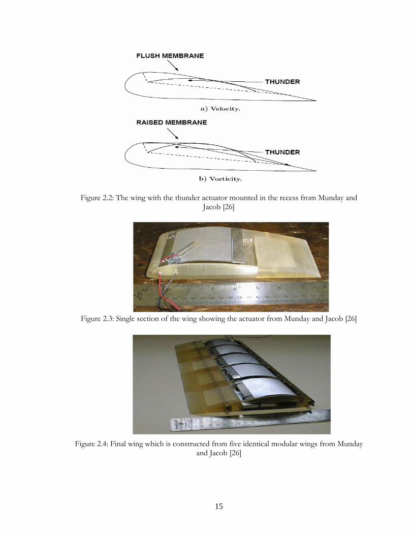
can be seen in figure 2.3 and five identical sections are placed side by side to construct and
entire wing (figure 2.4).
15
Figure 2.2: The wing with the thunder actuator mounted in the recess from Munday and Jacob [26]
Figure 2.3: Single section of the wing showing the actuator from Munday and Jacob [26]
Figure 2.4: Final wing which is constructed from five identical modular wings from Munday
and Jacob [26]

16
A single wing section is about 8 inches in chord length and 3.25 inches in width
which made the final wing module 17 inches ( 3.25” x 5) in length. The operating range of
the THUNDER 1 actuator is -300V to +600V and it produces a one centimeter deflection at
the tip [26]. This actuator has a maximum range of displacement at a frequency of
approximately 25 Hz. Further details about the wing construction can be obtained in
Munday and Jacob [26].
The base profile chosen for the current wing construction is NACA 4415 because it
provides sufficient thickness to place the actuator assembly into the airfoil and it is relatively
a flat bottomed airfoil.
2.3 Wind Tunnel Description
The wind tunnel used for this study is a Low-Speed, Low-Turbulence, open-circuit
blow-down wind tunnel and has a radial fan which is powered by a 7.5 Hp motor. Flow
conditioning is obtained by a flow straightener, turbulence damping screens, and a vibration
damper. Maximum velocity that can be obtained in the test section is 35m/s and it is
constructed from 0.25” thick polycarbonate and has a 3 component balance for lift, drag,
and pitching moment measurements [26]. Other physical details about the wind tunnel can
be obtained in [26]
Measurements regarding the separated region are obtained by flow visualization.
Details regarding the smoke wire technique can be obtained elsewhere [26]. As the upstream
portion of the flow is laminar, the point at which the streak-lines nearer to the surface begin
to break down, then that point gives us the location of transition. For PIV, the laser sheet
was generated by a 25mJ double-pulsed Nd:YAG laser with a maximum repetition rate of 15
Hz. Pulse separations varied from 100 micro-s to 1ms based upon the tunnel velocity. A 10

17
bit CCD camera with a 1008x1018 pixel array was used to capture images [33]. Uniform
seeding was accomplished using 1 micron oil droplets. A predictor-corrector algorithm with
an interrogation area of 32x32 was used to generate displacement vectors and velocity
gradients. For each PIV run, at least 200 images were recorded for processing, resulting in a
minimum of 100 vector and vorticity fields from which to generate statistics [34].
2.4 Results by Munday and Jacob
With of application of the current technology Munday and Jacob [26] observed the
decrease in separation at Reynolds number of 25,000 and angles of attack of 00 and 90 which
is evident from the figure 2.5 and 2.6. The oscillating frequency applied for the actuator in
these two cases is 15 Hz and 45 Hz respectively. Figure 2.7 shows the separated flow
thickness with respect to angle of attack at two different Reynolds number for actuated and
unactuated cases, clearly demonstrating that the separation is decreasing for actuated cases in
comparison to unactuated cases. PIV realizations of their study regarding flow separation
can be found elsewhere [26, 27, 34]. Their experiments also revealed that runs at Re =
25,000 and 50,000 are purely laminar and they were not sure about the laminar behavior at
Re = 100,000. They extended their work to numerically simulate the flow pattern [27] and
some of the preliminary results obtained by them are shown in figures 2.8 and 2.9. All the
preliminary work done from a numerical stand point is for unactuated cases and in an 8x16
inch wind tunnel (8 inches height and 16 inches depth). Their preliminary numerical
simulations showed that runs at Re = 25,000 at AoA = 00, 30 are periodic in nature and
another run at Re = 50,000 and AoA = 00 is quasi periodic. Runs at Re = 25,000 did not
showed at vortex formation with in the range of in between 30% to 70% of chord length
which was in agreement with the experimental results. The simulations predicted a smaller

18
separation region in comparison with experiments in three preliminary runs. For Re =
50,000 and AoA = 00 vortex formation was seen in between 30% to 70% of the chord
length which is in agreement with experimental results.
a) No Actuation
b) Actuation at f = 15 Hz
Figure 2.5: Streamlines at Re = 25,000 and AoA = 00 from Munday and Jacob [26]
a) No Actuation
b) Actuation at f = 45 Hz.
Figure 2.6: Streamlines for Re = 25,000 and AoA = 90 from Munday and Jacob [26]

19
Figure 2.7: Separated flow thickness for static and dynamic cases from Munday and
Jacob [33]
Figure 2.8: Instantaneous CFD vorticity for Re = 25,000 and AoA = 00 from
Munday et al [27]
Figure 2.9: Average CFD vorticity for Re = 25,000 and AoA = 00 from Munday et al
[27]
20
The present research continues the numerical study done by Munday and Jacob and
extends it to the simulation of actuated cases along with filling most of the parameter space
in unactuated cases. As the present research emphasizes performing numerical simulations,
detailed investigations have been done regarding grid study, time step length and effect of
transition model. Subsequent chapters will provide further detail on the remaining issues.
2.5 CFDVAL
CFD simulations are gaining importance in the field of flow control and codes used
for these simulations should be validated for accuracy against challenging test cases in order
to have greater trust in the results obtained from those codes. The CFD code used in the
present research has been validated against a challenging test case through participation in a
CFD workshop.
The workshop was titled “CFD Validation of Synthetic Jets and Turbulent
Separation Control” which was an International workshop organized by NASA Langley
Research Center in March, 2004. The purpose of this workshop was to bring together a
leading international group of computational fluid dynamics practitioners to assess the
current capabilities of different classes of turbulent flow solution methodologies to predict
flow fields induced by synthetic jets and separation control geometries.
Out of three test cases presented in the workshop the test case used for the present
study is the third one which was titled as “Flow over a Hump Model (Actuator Control)”.
This hump model was regarded as one of the challenging test cases from CFD point of view
and much previous work has been done on this type of model from an experimental stand
point by Seifert and Pack [35, 36 and 37].

21
2.5.1 Previous Work
In their first paper Seifert and Pack [35] conducted the experiments in a cryogenic
pressurized wind tunnel on wall-mounted bump. The Reynolds number range they used is
from 2.4 x 10⁶ to 26 x 106. The model they have was similar to the upper surface of a 20%
thick Glauert-Goldschmied-type airfoil at zero incidence. Separation control was tested using
steady suction, steady blowing, and actuator control. The actuator used here simulates the
combination of suction and blowing. They determined that the boundary layer was turbulent
through out the length of the hump. Reduction in 43% of the boundary-layer momentum
thickness upstream of the leading edge had a small effect on baseline separation. Steady
suction or blowing with a momentum coefficient of about 2% to 4% was required to fully
attach the flow to the model. Use of active excitation resulted in the same effectiveness as
suction control and was better than blowing.
In extending their research Seifert and Pack [36] explored the effects of mild sweep
on active separation control for incompressible Mach numbers. The sweep angles they have
tested were 00 and 300. They found that the excitation should be introduced slightly upstream
of the separation region regardless of the sweep angle. The effectiveness when the excitation
slot located at x/c = 0.64 was higher than the slot located at x/c = 0.59 (x represents x axis
and c represents chord length).
Seifert and Pack [37] also studied the effects of compressibility and excitation for
Reynolds numbers from 1.1 x 10⁷ to 3 x 10⁷ and for different Mach numbers. They found
that blowing becomes more effective that suction at transonic speeds and opposite was seen
in low Mach numbers. At compressible speeds they found that the presence of the excitation
slot at x/c = 0.59 alters the pressure distribution and separation location.

22
The work done by Seifert and Pack resulted in numerous numbers of results with
different parameters which provide challenging data for numerical simulations. The present
test case is a slight modification of the experiments performed by Seifert and Pack whose
description is as follows.
2.5.2 Experimental Description
The present model is also a wall-mounted Glauert-Goldschmied type body,
geometrically similar to that employed by Seifert & Pack [35, 36, and 37]. The model is
mounted between two glass endplates and both leading edge and trailing edges are faired
smoothly with a wind tunnel splitter plate as depicted in figure [2.10, 2.11]. Given the
exception of the side wall effects, the present experiment is a two dimensional experiment.
The tunnel dimensions at the test section are 28 inches wide by 20 inches high, but the
hump model is mounted on a splitter plate (0.5 inches thick), yielding a nominal test section
height of 15.032 inches (distance from the splitter plate to the top wall). The splitter plate
extends 76.188 inches upstream of the model's leading edge. Also, 44.437 inches
downstream of the model's leading edge, the splitter plate is equipped with a flap (3.75
inches long), which is deflected up during the experiment in order to control the air flow
beneath the splitter plate. This control affects the stagnation point at the leading edge of the
splitter plate, avoiding massive separation in that region [38].
Figure 2.10: Complete view of the experimental model [38]

23
Figure 2.11: Cartoon from Greenbalt et al [39]
Figure 2.12: Experimental setup from Greenbalt et al [39]
The characteristic reference length of the model is defined here as the length of the
bump on the wall, 16.536 inches. Their leading edge was then faired smoothly into the wall
from x = -.3937 to x = .3937 inches; however this additional length ahead of x = 0.0 was not
accounted for in their definition of the reference length. For the current experiment the
leading edge smoothing was not considered separately hence the actual bump length is
considered as the reference length. But Seifert and Pack [35] did not include leading edge
Glass
Flow Direction
Endplates

24
smoothing in the reference length making the current model slightly different than that of
Seifert and Pack model.
The model itself is 23 inches wide between the endplates at both sides (each endplate
is approximately 9.25 inches high, 34 inches long, and 0.5 inches thick with an elliptical-
shaped leading edge). The model is 2.116 inches high at its maximum thickness point. Both
uncontrolled (baseline) and controlled flow scenarios are considered under the conditions of
M = 0.1 and Re somewhat less than 1 million per chord. The tunnel medium is air at sea
level. The model experiences a fully-developed turbulent boundary layer whose delta
(thickness) at the leading edge of the model is between 1 and 2 inches. The boundary layer is
subjected to a favorable pressure gradient over the front convex portion of the body and
separates over a relatively short concave section in the aft part of the body. A slot at
approximately the 65% chord station on the model extends across the entire span of the
hump. Flow control is supplied by way of the two-dimensional slot across the span,
immediately upstream of the concave surface. This control uses steady suction, which is
driven by a suction pump with the mass flow monitored. Additional flow control may also
include zero mass-flux oscillatory suction/blowing [38].
Figure 2.13: Experimental details from Greenbalt et al [39]

25
2.5.3 Experimental Details [38]:
The conditions at which the experiments were conducted are listed below.
Ambient Pressure = 101325 kg/ (m-s2) Ambient Temperature = 298 K
Ambient Density = 1.185 kg/m3
Ambient Viscosity = 18.4 x 10⁻⁶ kg/m-s
Free stream velocity = 34.6 m/s
Reynolds Number = 9.36 x 10⁵ per chord length (16.536 inches)
The results from CFD simulations in comparison with the experiments for the present
test case will be presented in chapter 4.

26
__________ CHAPTER
3 __________
COMPUTATIONAL TOOLS
This chapter provides a brief description of the various computational tools used in
this thesis. Most of the computations performed in this research are done using GHOST, a
two dimensional structured code. Some of the computations involving the case described in
chapter 4 are done with UNCLE, a two/three dimensional unstructured CFD code.
3.1 Introduction
Of the two codes used in this study, GHOST is the more established, having been
used for example in a number of published analyses of transitional turbomachinery flows
and active flow control [41- 46]. UNCLE is a relatively new code intended to test aspects of
parallel unstructured code design as well as be a practical code for engineering applications
[47, 48]. Despite their differing structures, UNCLE and GHOST share several common

27
approaches to solving the Navier-Stokes equations. A brief description of the solver
methodology for these two codes is presented here.
3.2 Description of GHOST
GHOST is two-dimensional incompressible finite-volume structured computational
fluid dynamics code with chimera overset grids for parallel computing. The QUICK scheme
is applied to discretize the advective terms in the momentum equations with second-order
accuracy. A second-order central difference scheme is used for the diffusive terms. For the
RANS turbulence equations, the Total Variation Diminishing (TVD) scheme is employed
for the advective terms. Interfacial fluxes are determined through interpolation of cell-
centered values. Second order upwind time discretization is employed for the temporal
terms, using a delta-form subiterative scheme. GHOST is written in FORTRAN90 and has
been ported to a wide variety of platforms. GHOST was also designed to minimize memory
usage, accomplished through extensive use of the allocation and de-allocation of variables in
FORTRAN90. GHOST uses a cell-centered partitioning approach, and the internode
communication protocol is MPI. GHOST has mechanisms to do a form of automatic load
balancing.
Flow and geometry data in GHOST for a given grid or subgrid are stored in
individual arrays, as in φ B1 B(i,j), φB2B(i,j), …. φ Bn B(i,j). On a given grid, GHOST performs the
majority of its calculations as a series of i,j bi-directional sweeps in nested double loops. In
brief, the momentum equations are solved implicitly in a delta form, shown here for the time
discretization in one dimension:

28
xf
tt
xf
tmnnmnnn
mm
∂∂
−∆
−−
∆−
=∂∆∂
+∆∆
++− ))((2
))((32
)(
)(2
)(3
111 φφφφφ
φφ
(3.1)
where φ represents any variable, m is the subiteration level, and n is the time iteration
level. The right-hand side of Eq. (3.1) is explicit and can be implemented in a straightforward
manner to discretize the spatial derivative term. The left-hand side terms are evaluated based
on the first order upwind differencing scheme. The deferred iterative algorithm is strongly
stable, and the solution φP
n+1P is obtained by using inner iterations to reach the convergent
solution of the right-hand side of Eq. (3.1), corresponding to ∆φ approaching zero. At least
one subiteration is performed at every time step so that this method is fully implicit.
Matrices which are generated at each subiteration based on the QUICK and TVD
schemes are solved with ADI-type decomposition by making a pair of sweeps alternately in
the i- and j-directions which are solved sequentially in tri-diagonal matrices. Evaluation of
source/sink terms is done in the same process. This sequence may be repeated for improved
accuracy. The techniques of Rhie and Chow [49]P
Pare then used to extract the pressure field.
Three turbulence options in GHOST are applicable to this project. The first is to
assume fully laminar flow; the second is fully turbulent flow using Menter’s SST two-
equation model [50]; the third is to employ the transition model of Suzen et al. [43, 51] in
conjunction with the Menter SST model, a combination which has been found to provide
improved predictive capability for transitional flows with separation. In the transitional and
fully turbulence, an inflow turbulence of 1% is assumed. Details about the boundary
conditions present in GHOST and their description can be obtained from appendix A2.

29
3.3 Description of UNCLE [48]
UNCLE is another in house code developed by P.G. Huang at University of
Kentucky. As mentioned earlier some of the computations which are presented in chapter 4
were done with UNCLE in order to compare the results obtained from GHOST and
UNCLE so that these two codes can be validated against the experimental results of a
challenging test case. UNCLE is an in-house CFD code designed to meet the challenges of
using the unstructured grid codes on high-performance parallel computers. It is a two/three-
dimensional finite volume unsteady incompressible Navier-Stokes solver with cell-centered
pressure based SIMPLE algorithm. The code is second-order accurate in both time and
space. To increase flexibility in complex geometries, a cell-centered pressure-based method is
extended to use a variety of grid types, such as triangular, quadrilateral, tetrahedral, and
hexahedral meshes. To obtain good load balancing across computational nodes, METIS [52]
is applied for domain decomposition. METIS is a set of programs for partitioning graphs
and finite element meshes, and for producing fill-reducing orderings for sparse matrices. The
algorithms implemented in METIS are based on multilevel graph partitioning schemes. The
key features of METIS include extremely fast partition, high quality partitions, and low fill
orderings. The parallel construction of UNCLE is based on message passing interface (MPI)
protocols and has worked successfully on systems ranging from commodity PC clusters up
to traditional supercomputers. Accuracy and performance of the cell-centered pressure-
based method are demonstrated by various test cases in [48]. All test cases performed using
UNCLE were fully turbulent and we used Menter’s SST turbulence model for those cases.
Detailed description of SST [51] turbulence model can be obtained in appendix A1.

30
3.4 Hardware and Computation details
All the computations are performed in the commodity clusters KFC1, KFC2, and
KFC4 at UKCFD lab in University of Kentucky. KFC1 consists of 20 dual AMD nodes.
Each node has two 1.4 GHz Athlon MP Processors with 384 MB main memory per
processor and 40 GB of disk space for each node. KFC2 is made up of 50 AMD nodes, each
one having 2000+ XP Athlon processor and 256 MB main memory. KFC4 has 46 nodes
and each one has a Barton AMD 2500+ processor. On the baseline grid of about 85,000
points and a baseline dimensionless timestep of ∆t = 0.0001 with 10 subiterations on KFC4,
the runtime was about 12 hours (walltime) per dimensionless time unit ( ∞uc / ) for laminar
simulations and 21 hours for transitional simulations.

31
__________ CHAPTER
4 __________
VALIDATION OF CODES AGAINST A HIGH-RE TEST CASE
This chapter deals with the CFD simulation of a test case aimed at the validation of
the present generation CFD codes, therefore from an experimental point of view this test
case was chosen in such a way as to be numerically challenging. The experimental details for
this test case were explained in chapter 2. The codes validated with this test case are
GHOST and UNCLE whose description is already given in chapter 3. This chapter contains
the details about the grid setup, quantities calculated, and results obtained through
simulations.
4.1 Introduction
The present test case is a flow control test case but at high Reynolds numbers as
opposed to low Reynolds numbers used in the research presented in this thesis. Present

32
validation will help to demonstrate that the code used for the research in this thesis can lead
us to good results in all respects. The validated codes with the present test case are GHOST
and UNCLE but the main emphasis here is on GHOST because of its usage in this research.
This test case has been further divided into two cases. One is the baseline case with no flow
control mechanism and another one is with steady suction through the slot at 65% of the
chord length of the hump. The steady suction velocity examined was 0.01518 kg/s which
does not totally eliminate the separation bubble but does reduce the size of the separation
bubble. The two cases will be referred to as the baseline (no suction) and suction case.
Baseline cases were simulated using GHOST and suction cases were simulated using
GHOST and UNCLE, therefore the results for the suction case contains the plots from
GHOST and UNCLE in comparison with the experimental results.
4.2 Experimental Conditions [38]
The conditions at which the experiments were conducted are listed below.
Ambient Pressure = 101325 kg/ (m-s2)
Ambient Temperature = 298 K
Ambient Density = 1.185 kg/m3
Ambient Viscosity = 18.4 x 10⁻⁶ kg/m-s
Free stream velocity = 34.6 m/s
Reynolds Number = 9.36 x 10⁵ per chord length (16.536 inches)
4.3 Quantities Calculated
The coefficient of pressure, Cp, which is generally considered as the quantity which
can be obtained from the experiments with minimum error is one of the primary quantity to

33
be compared with the experimental results. The definition of Cp considered in experiments
and simulations is given in equation 4.1.
( )22/1 refref
refp u
ppc
ρ
−= (4.1)
Where refρ = 1.185 kg/m^3 refu = 34.6 m/s
Other quantities taken for the comparisons with the experimental results are u and v
velocities at the specified positions shown in figure 4.1. Turbulent quantities such as
turbulent shear stress, turbulent normal stress in horizontal direction, and turbulent normal
stress in vertical direction at specified position in figure 4.1 are also taken for comparison in
both the cases.
X/C
Y/C
0 0.5 1 1.50
0.1
0.2
0.3
0.4
0.5
0.6
0.7
0.8
0.650.66
0.80.9 1.0
1.1 1.2 1.3
Figure 4.1: Locations where velocities and turbulent quantities are measured
4.4 Grid and Boundary Conditions
Figure 4.2 shows the computational grid used for the numerical simulations. The
total number of grid points for this grid are 199,427 and it consists of nine zones.

34
Specifying the boundary conditions proved to be a key challenge in this case. The
upstream portion of the grid until x/c = -2.14 was not included in the numerical simulations
because u velocity profile and streamwise turbulent intensity values were given as an inlet
boundary condition from the experiments. Several boundary conditions such as inviscid wall,
freestream, and no-slip wall were tested for the slot portion of the grid and finally no-slip
wall was used for no suction case in the current computation. The remaining boundary
conditions can be seen in figure 4.3
For this case most of the simulations were performed in the steady-state mode and
turbulent stress values are obtained from time dependent runs where the time step is 0.001.
The steady-state runs are done for a sufficient number of iterations until the flow data has
converged to a constant solution.
x/c
y/c
-2 -1 0 1 2 3 40
1
2
3
4
5
x/c
y/c
0 0.5 1-0.2
-0.1
0
0.1
0.2
0.3
0.4
0.5
0.6
0.7
0.8
0.9
1
1.1
1.2
x/c
y/c
0.6525 0.655 0.6575 0.660.111
0.112
0.113
0.114
0.115
0.116
0.117
0.118
0.119
0.12
0.121
0.122
Figure 4.2: Grid used for the computation purpose which is made up of nine zones

35
Figure 4.3: Boundary conditions used for the present numerical simulations
4.4.1 Inlet Boundary Conditions
The original test section is about 76.188 inches from the leading edge of the model.
In order to eliminate modeling the total test section in the CFD solution the velocity profile
at 38.387 inches upstream of the leading edge is obtained from the experiments. A flat plate
test case is run to match the Reθ obtained from the experiments and the turbulent quantities
obtained from the flat plate test case are used for the inlet boundary condition which is
38.387 inches upstream of the leading edge of the hump. Fig 4.4 shows the velocity profile
obtained from flat plate in comparison with the experimental profile.
4.4.2 Grid Independence
Grid Independence has been examined using two different grids. Grid one consists of
50,227 grid points with five zones and grid two consists of 199,427 grid points with nine
zones. Figure 4.5 shows the Cp over the hump using these two grids in comparison with

36
experimental results. The similarity of the two results shows that grid independence has been
reached.
U /U inf
Y/C
0 .5 0 .6 0 .7 0 .8 0 .9 1
0
0.02
0.04
0.06
0.08
0 .1
0 .12
0.14
0.16 E xpe rim e nta l P rofileF la t P la te P rofile
Figure 4.4: Inlet velocity profile from experiment and flat plate test case
x/c
Cp
-1 0 1 2
-1
-0.9
-0.8
-0.7
-0.6
-0.5
-0.4
-0.3
-0.2
-0.1
0
0.1
0.2
0.3
0.4
0.5
ExperimentComputation Grid 1
x/c
Cp
-1 0 1 2
-1
-0.9
-0.8
-0.7
-0.6
-0.5
-0.4
-0.3
-0.2
-0.1
0
0.1
0.2
0.3
0.4
0.5
ExperimentComputation Grid 2
Figure 4.5: Cp plots in comparison with experimental results for two different grids
4.5 Results
Huge data sets are generated by the experiments which including a large amount of
turbulent data. In order to have effective comparison between the experimental and
numerical results all the data obtained from the experiments has been compared with the
numerical results, yielding an awkwardly large number of data sets. In order to have better
understanding of the data it has been divided into groups based on its nature. These

37
categories of data with corresponding figure numbers and brief comments from these
comparisons can be found in tables 4.1 and 4.2.
4.5.1 Base line case
The presented results for the baseline case are simulated using GHOST and these are
plotted in comparison with the experimental results. Table 4.1 shows the plots presented for
this case and the comment of that plot accompanied by the figure number.
Table 4.1 : Various quantities used for the comparison, corresponding figure number and
brief comments for the baseline case.
Category Comment Figure #
Cp plot
Has the good comparison along the upstream
of the slot and predicts higher separation
bubble.
4.6
Separation bubble Numerical simulations predicted larger
separation bubble. The variation between
experiments and simulations is 0.1 (∆x/c)
4.7
Velocity plots Shows u-velocity and v-velocity plots at
different locations. Plots at x/c = 1.1 and 1.2
clearly depicts that separation bubble in
numerical simulations is higher. This can be
attributed to the turbulence model used in the
current computations.
4.8

38
Turbulence
Shear stress
Numerical simulations produced the same
trend but could not correctly estimate the
values of shear stress.
4.9
Turbulent
normal stress
in horizontal
direction
Normal stress also shows the same behavior
as that of shear stress i.e it could not be
correctly estimated but we could obtain the
same trend as that of experiments.
4.10
Turbulence
plots Turbulent
normal stress
in vertical
direction
Except at two locations (x/c = 0.65 and 0.66)
we could correctly estimate the normal stress
values. Improper estimation at x/c = 0.65 and
0.66 can be attributed to the their location,
which is very much nearer to the slot region
4.11
4.5.2 Suction case
Simulations for the suction case are done using both the CFD codes, GHOST and
UNCLE, and the results from these codes are presented in comparison with the
experimental results. Table 4.2 shows the list of various figures presented for this case
accompanied by some brief comments on these results. Simulation results from GHOST
and UNCLE showed a great similarity with each other for various quantities collected.

39
Table 4.2 : Various quantities used for the comparison, corresponding figure number and
brief comments for the suction case.
Category Comment Figure #
Cp plot
This plot clearly shows the effect of suction on the
separation bubble, but simulations over predicted
the size of the separation bubble.
4.12
Separation bubble Larger separation bubble was obtained in numerical
simulations. The variation is 0.15 (∆x/c)
4.13
Velocity plots These plots show the numerical simulations did not
predict the correct u and v velocity values but we
could obtain the correct trend as that of
experiments. The deviation is mainly because of the
over prediction of the separation bubble.
4.14
Turbulent
Shear
stress
Same trend as that of experiments can be obtained
but the correct magnitudes could not be obtained
through numerical simulations.
4.15
Turbulence
plots
Turbulent
normal
stress in
horizontal
direction
Normal stress also shows the same behavior as that
of shear stress i.e it could not be correctly estimated
but we could obtain the same trend as that of
experiments.
4.16

40
Turbulent
normal
stress in
vertical
direction
In base line case except for two positions we could
almost catch the behavior of experiments but in
suction we were some what deviating from the
experimental results.
4.17

41
4.5.3 Figures related to Baseline case
x/c
Cp
-1 0 1 2
-1
-0.9
-0.8
-0.7
-0.6
-0.5
-0.4
-0.3
-0.2
-0.1
0
0.1
0.2
0.3
0.4
0.5
ExperimentComputation
Figure 4.6: Experimental and Computation(GHOST) Cp for baseline case
X/C
Y/C
0.6 0.8 1 1.2 1.4-0.1
0
0.1
0.2
0.3
0.4
0.5
Figure 4.7: Separation bubble for baseline case from GHOST

42
U/Uinf , V/Vinf
y/c
-0.5 0 0.5 1 1.50.1
0.11
0.12
0.13
0.14
0.15
0.16
0.17
0.18
0.19
0.2
x/c=0.65
U/Uinf , V/Vinf
y/c
-0.5 0 0.5 1 1.50.1
0.11
0.12
0.13
0.14
0.15
0.16
0.17
0.18
0.19
0.2
x/c=0.66
U/Uinf , V/Vinf
y/c
-0.5 0 0.5 1 1.50
0.05
0.1
0.15
0.2
x/c=0.8
U/Uinf , Vinf
y/c
-0.5 -0.25 0 0.25 0.5 0.75 1 1.25 1.50
0.05
0.1
0.15
0.2x/c=0.9
U/Uinf , V/Vinf
y/c
-0.5 0 0.5 1 1.50
0.05
0.1
0.15
0.2
x/c=1.2
U/Uinf , V/Vinf
y/c
-0.5 0 0.5 1 1.50
0.05
0.1
0.15
0.2
x/c=1.3
U/Uinf , V/Vinf
y/c
-0.5 -0.25 0 0.25 0.5 0.75 1 1.25 1.50
0.05
0.1
0.15
0.2x/c=1.0
U/Uinf , V/Vinf
y/c
-0.5 0 0.5 1 1.50
0.025
0.05
0.075
0.1
0.125
0.15
0.175
0.2
x/c=1.1
U-Velocity (Computation)V-Velocity (Computation)U-Velocity (Experiment)V-Velocity (Experiment)
Figure 4.8: U and V velocities at different locations on the hump from GHOST
(computation) in comparison with experimental results for the baseline case
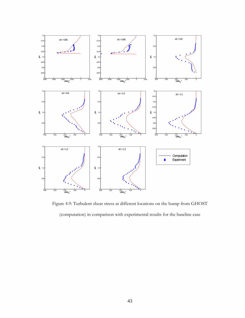
43
UV/Uinf2
y/c
-0.004 -0.003 -0.002 -0.001 0 0.0010
0.025
0.05
0.075
0.1
0.125
0.15
0.175
0.2
x/c=0.65
ComputationExperiment
UV/Uinf2
y/c
-0.004 -0.003 -0.002 -0.001 0 0.0010
0.025
0.05
0.075
0.1
0.125
0.15
0.175
0.2
x/c=0.66
UV/Uinf2
y/c
-0.04 -0.03 -0.02 -0.01 00
0.05
0.1
0.15
0.2
x/c=0.8
UV/Uinf2
y/c
-0.04 -0.03 -0.02 -0.01 00
0.05
0.1
0.15
0.2x/c=0.9
UV/Uinf2
y/c
-0.04 -0.03 -0.02 -0.01 00
0.05
0.1
0.15
0.2x/c=1.0
UV/Uinf2
y/c
-0.04 -0.03 -0.02 -0.01 00
0.025
0.05
0.075
0.1
0.125
0.15
0.175
0.2
x/c=1.1
UV/Uinf2
y/c
-0.04 -0.03 -0.02 -0.01 00
0.05
0.1
0.15
0.2
x/c=1.2
UV/Uinf2
y/c
-0.04 -0.03 -0.02 -0.01 00
0.05
0.1
0.15
0.2
x/c=1.3
Figure 4.9: Turbulent shear stress at different locations on the hump from GHOST
(computation) in comparison with experimental results for the baseline case

44
UU/Uinf2
y/c
0 0.005 0.010
0.025
0.05
0.075
0.1
0.125
0.15
0.175
0.2
x/c=0.65
UU/Uinf2
y/c
0 0.005 0.010
0.025
0.05
0.075
0.1
0.125
0.15
0.175
0.2
x/c=0.66
UU/Uinf2
y/c
-0.01 0 0.01 0.02 0.03 0.04 0.05 0.060
0.05
0.1
0.15
0.2
x/c=0.8
UU/Uinf2
y/c
-0.01 0 0.01 0.02 0.03 0.04 0.05 0.060
0.05
0.1
0.15
0.2x/c=0.9
UU/Uinf2
y/c
-0.01 0 0.01 0.02 0.03 0.04 0.05 0.060
0.05
0.1
0.15
0.2x/c=1.0
UU/Uinf2
y/c
-0.01 0 0.01 0.02 0.03 0.04 0.05 0.060
0.025
0.05
0.075
0.1
0.125
0.15
0.175
0.2
x/c=1.1
UU/Uinf2
y/c
-0.01 0 0.01 0.02 0.03 0.04 0.05 0.060
0.05
0.1
0.15
0.2
x/c=1.2
UU/Uinf2
y/c
-0.01 0 0.01 0.02 0.03 0.04 0.05 0.060
0.05
0.1
0.15
0.2
x/c=1.3
ComputationExperiment
Figure 4.10: Turbulent normal stress in horizontal direction at different locations on the
hump from GHOST (computation) in comparison with experimental results for the baseline
case

45
VV/Uinf2
y/c
0 0.005 0.010
0.025
0.05
0.075
0.1
0.125
0.15
0.175
0.2
x/c=0.65
VV/Uinf2
y/c
0 0.005 0.010
0.025
0.05
0.075
0.1
0.125
0.15
0.175
0.2
x/c=0.66
VV/Uinf2
y/c
-0.01 0 0.01 0.02 0.03 0.04 0.05 0.060
0.05
0.1
0.15
0.2
x/c=0.8
VV/Uinf2
y/c
-0.01 0 0.01 0.02 0.03 0.04 0.05 0.060
0.05
0.1
0.15
0.2x/c=0.9
VV/Uinf2
y/c
-0.01 0 0.01 0.02 0.03 0.04 0.05 0.060
0.05
0.1
0.15
0.2x/c=1.0
VV/Uinf2
y/c
-0.01 0 0.01 0.02 0.03 0.04 0.05 0.060
0.025
0.05
0.075
0.1
0.125
0.15
0.175
0.2
x/c=1.1
VV/Uinf2
y/c
-0.01 0 0.01 0.02 0.03 0.04 0.05 0.060
0.05
0.1
0.15
0.2
x/c=1.2
VV/Uinf2
y/c
-0.01 0 0.01 0.02 0.03 0.04 0.05 0.060
0.05
0.1
0.15
0.2
x/c=1.3
ComputationExperiment
Figure 4.11: Turbulent normal stress in vertical direction at different locations on the hump
from GHOST (computation) in comparison with experimental results for the baseline case

46
4.5.4 Figures related to Suction Case
x/cC
p
-1 0 1 2
-1
-0.8
-0.6
-0.4
-0.2
0
0.2
0.4
x/c
Cp
-1 0 1 2
-2
-1.5
-1
-0.5
0
0.5
Experiment SuctionGhost coarse SuctionUncle coarse Suction
Figure 4.12: Cp for the suction case from GHOST and UNCLE in comparison with
experimental data
X /C
Y/C
0.6 0 .8 1 1.2 1 .4-0 .1
0
0.1
0 .2
0 .3
0 .4
0 .5
Figure 4.13: Separation bubble for suction case from GHOST

47
U/Uinf, V/Uinf
y/c
-0.5 0 0.5 1 1.50.1
0.11
0.12
0.13
0.14
0.15
0.16
0.17
0.18
0.19
0.2
x/c=0.65
U/Uinf, V/Vinf
y/c
-0.5 -0.25 0 0.25 0.5 0.75 1 1.25 1.50.1
0.11
0.12
0.13
0.14
0.15
0.16
0.17
0.18
0.19
0.2
x/c=0.66
U/Uinf, V/Vinf
y/c
-0.5 0 0.5 1 1.50
0.05
0.1
0.15
0.2
x/c=0.8
U/Uinf, V/Uinf
y/c
-0.5 0 0.5 1 1.50
0.05
0.1
0.15
0.2
x/c=1.2
U/Uinf, V/Uinf
y/c
-0.5 0 0.5 1 1.50
0.05
0.1
0.15
0.2
x/c=1.3
U/Uinf , V/Uinf
y/c
-0.5 0 0.5 1 1.50
0.05
0.1
0.15
0.2
x/c=0.9
U/Uinf , V/Uinf
y/c
-0.5 0 0.5 1 1.50
0.05
0.1
0.15
0.2x/c=1.0
U/Uinf, V/Uinf
y/c
-0.5 0 0.5 1 1.50
0.05
0.1
0.15
0.2
x/c=1.1
Ghost(U-velocity)Ghost(V-velocity)Uncle(U-velocity)Uncle(V-velocity)Experiment(U-velocity)Experiment(V-velocity)
Suction
Figure 4.14: U and V velocities for suction case at different locations on the hump from
GHOST and UNCLE in comparison with experimental results.

48
UV/Uinf2
y/c
-0.004 -0.0035 -0.003 -0.0025 -0.002 -0.0015 -0.001 -0.0005 0 0.0005 0.0010
0.025
0.05
0.075
0.1
0.125
0.15
0.175
0.2
x/c=0.65
UV/Uinf2
y/c
-0.004 -0.003 -0.002 -0.001 0 0.0010
0.025
0.05
0.075
0.1
0.125
0.15
0.175
0.2
x/c=0.66
UV/Uinf2
y/c
-0.04 -0.03 -0.02 -0.01 0 0.010
0.05
0.1
0.15
0.2
x/c=0.8
UV/Uinf2
y/c
-0.04 -0.03 -0.02 -0.01 0 0.010
0.05
0.1
0.15
0.2
x/c=0.9
UV/Uinf2
y/c
-0.04 -0.03 -0.02 -0.01 0 0.010
0.05
0.1
0.15
0.2x/c=1.0
UV/Uinf2
y/c
-0.04 -0.03 -0.02 -0.01 0 0.010
0.05
0.1
0.15
0.2
x/c=1.1
UV/Uinf2
y/c
-0.04 -0.03 -0.02 -0.01 0 0.010
0.05
0.1
0.15
0.2
x/c=1.2
UV/Uinf2
y/c
-0.04 -0.03 -0.02 -0.01 0 0.010
0.05
0.1
0.15
0.2
x/c=1.3
Ghost (UVShearStress)Uncle(UVShearStress)Experiment (UVShearStress)
Suction
Figure 4.15: Turbulent shear stress for suction case at different locations on the hump from
GHOST and UNCLE in comparison with experimental results.

49
UU/Uinf2
y/c
0 0.005 0.010
0.025
0.05
0.075
0.1
0.125
0.15
0.175
0.2
x/c=0.65
UU/Uinf2
y/c
0 0.005 0.010
0.025
0.05
0.075
0.1
0.125
0.15
0.175
0.2
x/c=0.66
UU/Uinf2
y/c
0 0.05 0.10
0.05
0.1
0.15
0.2
x/c=0.8
UU/Uinf2
y/c
0 0.05 0.10
0.05
0.1
0.15
0.2
x/c=0.9
UU/Uinf2
y/c
0 0.05 0.10
0.05
0.1
0.15
0.2x/c=1.0
UU/Uinf2
y/c
0 0.05 0.10
0.05
0.1
0.15
0.2
x/c=1.1
UU/Uinf2
y/c
0 0.05 0.10
0.05
0.1
0.15
0.2
x/c=1.2
UU/Uinf2
y/c
0 0.05 0.10
0.05
0.1
0.15
0.2
x/c=1.3
Ghost(UUNormalStress)Uncle(UUNormalStress)Experiment(UUNormalStress)
Suction
Horizonaldirection
Figure 4.16: Turbulent normal stress in horizontal direction for suction case at different
locations on the hump from GHOST and UNCLE in comparison with experimental results.

50
VV/Uinf2
y/c
0 0.005 0.010
0.025
0.05
0.075
0.1
0.125
0.15
0.175
0.2
x/c=0.65
VV/Uinf2
y/c
0 0.005 0.010
0.025
0.05
0.075
0.1
0.125
0.15
0.175
0.2
x/c=0.66
VV/Uinf2
y/c
-0.01 0 0.01 0.02 0.03 0.04 0.05 0.060
0.05
0.1
0.15
0.2
x/c=0.8
VV/Uinf2
y/c
-0.01 0 0.01 0.02 0.03 0.04 0.05 0.060
0.05
0.1
0.15
0.2
x/c=0.9
VV/Uinf2
y/c
-0.01 0 0.01 0.02 0.03 0.04 0.05 0.060
0.05
0.1
0.15
0.2x/c=1.0
VV/Uinf2
y/c
-0.01 0 0.01 0.02 0.03 0.04 0.05 0.060
0.05
0.1
0.15
0.2
x/c=1.1
VV/Uinf2
y/c
-0.01 0 0.01 0.02 0.03 0.04 0.05 0.060
0.05
0.1
0.15
0.2
x/c=1.2
VV/Uinf2
y/c
-0.01 0 0.01 0.02 0.03 0.04 0.05 0.060
0.05
0.1
0.15
0.2
x/c=1.3
Ghost(VVNormalStress)UncleVVNormalStress)Experiment(VVNormalStress)
Suction
VerticalDirection
Figure 4.17: Turbulent normal stress in vertical direction for suction case at different
locations on the hump from GHOST and UNCLE in comparison with experimental results.

51
4.6 Results of other CFD codes in comparison to GHOST
In this section the results obtained by other CFD codes in the workshop are
presented in comparison with the results obtained by GHOST. For all the figures in this
section, UK-ghost-sst-1 and UK-ghost-sst-2 represents the results obtained by GHOST for
two different grids using SST turbulence model. Details regarding codes tested by other
participants at this workshop are as follows.
(i) In total 13 codes were used to test this case. (ii) Various turbulence models used
are based on RANS (Spalart-Allmaras, SST, k-e, k-o) (iii) Some participants used DNS. (iv)
Some participants used different boundary conditions to increase the accuracy
As this section is aimed at comparison of GHOST results with other CFD codes,
CFL3D a prominent code developed and widely used by NASA was taken into
consideration. For the present test case CFL3D was used with results obtained with the SST
turbulence model as are the results obtained using GHOST. The Cp plots from figure 4.18
(no suction case) are similar to the Cp plots obtained by CFL3D code and this hold true as
well for the suction case which is depicted in figure 4.19. Sample results for u velocity,
turbulent shear stress, and turbulent shear stress in the horizontal direction are presented in
figures 4.20, 4.21, and 4.22 respectively and the similarity between the GHOST results and
CFL3D results holds for these cases also.
Of the 13 codes presented in the workshop none of the codes could accurately
predict the experimental results, demonstrating and this shows that this is a challenging test
case.

52
Figure 4.18: Cp plots for Ghost results and other CFD code results from the workshop for
baseline case from CFDVAL2004 [38]
Figure 4.19: Cp plots for Ghost results and other CFD code results from the workshop for
suction case from CFDVAL2004 [38]
Figure 4.20: u-velocity plots for GHOST and other CFD codes at x/c =0.8 for baseline case
from CFDVAL2004 [38]

53
Figure 4.21: Turbulent shear stress for GHOST and other CFD codes at x/c =0.8 for
baseline case from CFDVAL2004 [38]
Figure 4.22: Turbulent normal stress in horizontal direction for GHOST and other CFD
codes at x/c =0.8 for baseline case from CFDVAL2004 [38]
4.7 Conclusions
The present computations with UNCLE and GHOST showed the similarity in
results despite the fact that UNCLE is an unstructured code and GHOST is a structured
code. Other CFD codes which have been used to solve the present case with the SST
turbulence model also showed the same results as that of GHOST and UNCLE. Results

54
from various other participants showed that k-ε turbulence model could somewhat more
accurately predict reattachment point for no suction case. Separation and reattachment
points predicted by all the turbulence models fall off from the experimental results,
clustering in a same region.
Cumulatively, the GHOST code performed at least as well as the well-established
codes long-used in the CFD community. Therefore, the results presented in the current
chapter validate the GHOST code with a challenging test case and hence it can be used for
wide variety of flow control applications with a reasonable degree of confidence.

55
__________ CHAPTER
5 __________
CASE SETUP AND RESULTS FOR NON-ACTUATING CASE
The validation of the proposed oscillatory flow control is done by performing
experiments and numerical simulations. Details about the experimental setup and wing
construction have already been discussed in chapter 2; this chapter deals with the
computational validation and investigation. Discussion in this chapter has been divided into
three parts. The first part deals with the brief description of test sections used for the
experiments. The second part deals with the numerical setup for the non-oscillatory airfoil
and an evaluation of the numerical time step and grid independence. The third part deals
with the non oscillatory case results from the numerical simulations and the comparison of
some of those results with experiments.

56
5.1 Experimental Details
The experiments for the present research were carried out by Munday and Jacob [26,
27]. The description of the wing construction and other details about their work has been
previously discussed in chapter 2. The parameters considered are Reynolds numbers whose
range is from 25,000 to 100,000 and angles of attack from 00 to 120 at an interval of 30.
The two wind tunnel sections used for the present experiments are the 8 x 16 inch
wind tunnel and 24x24 inch sections (figure 5.1). Preliminary numerical simulations and
experiments showed wall effects in the 8x16 inch wind tunnel section. Efforts to get
improved results from the 24x24 inch wind tunnels section are underway buy were not
completed in time for this thesis. As a result, the output of the present research is compared
to 8x16 inch test section data.
5.2 Cases The functioning of the present wing can be divided into two cases. The first case is
the static actuator case where the actuator present in the wing is not oscillating. The second
case is where the actuator will be oscillating at the given frequency. This frequency is
8 16
24
24
Figure 5.1: 8x16 and 24x24 inch experimental test sections

57
different for different test cases depending on the flow separation. Hence every static
actuator case will act as groundwork for morphing cases. The majority of the work presented
in this thesis deals with the static actuator cases followed by two oscillating actuator cases
where the separation was reduced by the use of oscillatory flow control. CFD set up of the
non-oscillating cases is explained in the following sections and the set up of non oscillating
cases are explained in chapter 6. Hence in brief the cases can be divided into
1. Static Actuator Cases
2. Dynamic Actuator Cases (Oscillating Actuator)
5.2.1 Static Actuator Case Setup
The computational tools used for this study have been explained in chapter 3 in
detail, therefore this section deals with the setup used for the computation. The wing used
for the numerical runs is shown in figure 5.2. The first set of experiments was conducted in
the 8x16 inch wind tunnel section hence the initial numerical simulations were performed in
the same size section. As the experiments switched to 24x24 inch test section computational
setup was also changed. Hence the following sections deal with the grid setup used for the
8x16 and 24x24 inch wind tunnel section and further sections show the justification of the
usage of 24x24 inch wind tunnel section.
Figure 5.2: Airfoil grid used for computations at AoA = 00
i j

58
5.2.2 Computation Domain
The computational grid is formed with the use of two-dimensional multi-zonal
blocks (figure 5.3, 5.4) .The grid defining the modified NACA 4415 airfoil is a single block
which overlaps the central background grid. This background grid is surrounded by eight
other rectangular grids. The dimensionless computational area is chosen according to the
desired experimental section. On the outer boundary, the left (inlet) boundary is fixed with a
uniform dimensionless inlet velocity ,0.1=∞u and the upper and lower boundary condition
are no-slip wall boundaries representing the top and bottom of the wind tunnel test section.
For the airfoil blocks, the inner boundary condition is a no-slip wall boundary condition, and
the outside boundary is set to “overlap” which allows the background grid points being
overlapped by the airfoil block grid points to interpolate values from the foreground airfoil
grid points. Computation information between adjacent blocks is exchanged by two ghost
points. All the parameters chosen in the computation are dimensionless. Care is taken to see
that the initial dimensionless y+ values of the airfoil grid are less than 0.5. The 8x16 inch grid
and 24x24 inch grid differ only in the computation region, which requires the 24x24 inch
grid to cover more area on the top and bottom of the airfoil grid.
Figure 5.3: Grid used for 8x16 inch wind tunnel section

59
x
y
-1 0 1 2 3-1.5
-1
-0.5
0
0.5
1
1.5
2
2.5
1
2 3 4
5 6 7
8 9 10
Figure 5.4: Grid used for 24x24 inch wind tunnel section
Table 5.1: Number of grid points used in each zone of the respective test sections.
(* two other grids were used for zone 1, both 300x120 with different configurations.)
8x16 inch test section 24x24 inch test section Zone i x j Zone i x j
1 155x80 1 155 x 80* 2 50x100 2 50 x 100 3 300x100 3 300 x 100 4 50x100 4 50 x 100 - - 5 50 x 40 - - 6 300 x 40 - - 7 50 x 40 - - 8 50 x 40 - - 9 300 x 40 - - 10 50 x 40

60
Simulations were performed on multiple commodity clusters at the University of
Kentucky (Kentucky Fluid Clusters 2, 4), typically on three processors (Barton AMD 2500+
processors on KFC4, 2000+ XP processors on KFC2). On the baseline grid of about 85,000
points and with a baseline dimensionless timestep of ∆t = 0.0001 with 10 subiterations on
KFC4, the runtime was 12 hours (walltime) per dimensionless time unit ( ∞uc / ) for laminar
simulations and 21 hours for transitional simulations.
5.3 Preliminary Studies
Three preliminary studies have been conducted in order to proceed further with the
numerical simulations. These studies are as follows:
1. Effect of boundary wall on the performance of airfoil
2. Effect of computational time step
3. Effect of Transitional model
For all the above mentioned cases the grid used for the airfoil was 155x80. This grid proved
to be reasonably adequate in subsequent grid independence studies, and as such these results
are assumed to accurately reflect these effects.
5.3.1 Study for the Effect of Wall
A shift from 8x16 inch test section to a 24x24 inch test section was justified in part
from the lift curves obtained from a run in both these test sections. Numerically, a change in
test section was achieved by increasing the distance above and below of the airfoil grid. A
sample result from this study can be seen in figure 5.5. In figure 5.5, c represents the chord
length which is 8 inches and the vertical height c represents the 8x16 inch test section where

61
as 3c represents the 24x24 inch test section. Similarly 4c and 6c represent the increase in the
vertical dimension of the section by a chord length and 3 chord lengths respectively.
Table 5.2: Dominant frequency with errors, average lift coefficient, and lift variation for
different test sections
Re = 25,000, AoA = 3o Test Section Frequency Cl H = c 2.62 ± 0.14 0.42± 0.18 H = 3c 1.68 ± 0.04 0.31± 0.10 H = 4c 1.71 ± 0.04 0.31± 0.13 H = 6c 1.73 ± 0.04 0.31± 0.12
In figure 5.5, the lift curves have been shifted so that their peaks nearest to t = 11
are aligned. Repeated simulations have demonstrated that by t = 8 – 10 the characteristic
nature of the flow is established, although in this paper to the extent possible data to be
compared will be presented at coincident simulation times. Both the amplitude and the
frequency of the subsequent flow are measurably altered by the 8 inch section compared to
the other heights, even though the qualitative behavior is similar. The remaining three
c
3c 4c
6c
c
3c 4c
6c
Figure 5.5: Cl curves for three different test sections at Re = 25,000 and AoA = 3o. The
curves have been shifted so that the peaks nearest t = 11 are aligned. On the right is a
graphical representation of the various test section heights relative to the airfoil section.

62
heights deviate somewhat from each other, but the overall amplitude and frequency of the
motion is quite similar. Hence, the results in this research will target simulations of the 24
inch test section.
Thomas and Salas [54] constructed a model to overcome the boundary effects (wall
effects) on the airfoil, but this model was limited to transonic flows. This model was based
on a supposition that the flow in the far field can be represented by linear small-disturbances
[54]. As the present simulations were targeted for comparison with experiment results,
inclusion of this far field model was not considered.
5.3.2 Effect of time step
Multiple timesteps have been tested in order to determine the effect of timestep on
these simulations. Figure 5.6 shows lift curves from simulations on the baseline grid with
Re=25,000 and AoA=3o for several dimensionless timesteps. In this figure, the initial peaks
are aligned. All the results are similar, but there are variations between each data set with no
clear pattern emerging. As such, a relatively conservative timestep of ∆t=0.0001 as the
baseline interval has been chosen.
Table 5.3: Dominant frequency with errors, average lift coefficient, and lift variation for
different time steps
Re = 25,000, AoA = 3o Time Step Frequency Cl 0.0001 1.68 ± 0.04 0.31± 0.10 0.0003 1.71± 0.06 0.32± 0.11 0.0005 1.64 ± 0.06 0.32± 0.13 0.0007 1.67 ± 0.06 0.31± 0.14

63
5.3.3 Effect of transition model
All the simulations were considered laminar at Reynolds number of 25,000 and the
remaining simulations were performed as laminar and turbulent with the inclusion of
transition model. The transition model used in this paper was developed by Suzen et al [43,
51]. This transition model is based on the addition of an intermittency equation and has been
thoroughly tested for turbine blade flows with Menter’s SST two-equation model. This
technique has generally shown excellent predictive capability for flows with separation.
At this time, there is no significant difference between the laminar and transitional
simulations (figures 5.7 and 5.8). This is because no reattachment point was evident from
transition simulations which would have been a critical difference between the laminar and
transition simulations. As evident in figure 5.8, when run with the SST turbulence model at
Re = 200,000 and AoA = 60 the flow exhibits state behavior, whereas laminar and transition
simulations still predict an oscillatory, time-dependent flow. The transitional model does
Figure 5.6: Variation of Re = 25000, AoA = 3o lift
curves with timestep. The peaks nearest to t = 5 have
been aligned for ease of comparison.

64
indicate transition is occurring at lower Reynolds numbers, but this has no noticeable effect
on the primary flow characteristics. Despite this, all the results for Reynolds number above
50,000 continued to use the transition model.
Figure 5.8: Cl plots for Laminar, Transition and Turbulent run at Re = 200,000 and
AoA = 60
5.4 Grid Study
The highly variable nature of these flows makes the assessment of grid independence
and similar characteristics a challenging task, so the approach used in this study is presented
here in greater detail. The first set of grid studies was performed on airfoil sections with
Figure 5.7: Instantaneous vortex plots and lift curves comparing the laminar (left) and transitional (right) simulations at Re=100,000 and AoA = 6o.

65
varying grid densities. A second set of simulations for flow over a cylinder on grid of
comparable densities was conducted to provide further insight into grid effects.
5.4.1 Variation in airfoil grid density
Previous studies of similar flows using GHOST have used airfoil or blade grids in
the range of 150-400 grid points to define the airfoil surface and 70-150 grid points in the
normal direction [41 - 46]. Based on this previous work several different grids were
considered for the current grid study as presented in table 5.4. While assessing true grid
independence is hampered by the strong time dependence of this flow, at Re=25,000 and
AoA=3o all the grids give similar results with the exception of the lift magnitude of the
outlier 300x160 grid. The effects are more significant with higher Reynolds number (figure
5.9), with the lowest resolution grid yielding a more periodic lift curve and lower lift values
than the higher resolution grids. However, it should be noted that the shift in lift values from
the Re=25,000 to Re=100,000 is in general significantly larger than the differences generated
by the changes due to grid density.
Figure 5.9: Cl curves for different airfoil grid resolutions at AoA = 3o for Re = 25,000
(left) and Re = 100,000 (right). Peaks nearest t = 20.5 and t = 8 are aligned for ease of
comparison.

66
5.4.2 Cylinder Cases
The variation shown with grid density has been further investigated by doing some
cylinder case runs, replacing the airfoil grid by cylinder grid in the same CFD setup (figure
5.11). Care has been taken such that the cylinder diameter coincides with the chord length of
the airfoil. The overall goal of these was to compare the Strouhal number obtained for
different cylinder grids with the collected experimental data from previous studies.
For this study three different grids have been chosen. The first grid was 155x80
which have been used extensively for all the results presented in Katam et al. [34]. Then two
other grids were produced in context with 155x80 grid by doubling i points and increasing
the j points to 120. The summary of the grids along with the differences in the last two grids
are as follows.
1. 155x80 (Grid 1): This grid has 155 points in i direction and 80 points in j
direction.
2. 310x120 (Grid 2): The 120 grid points in the j direction have been
clustered in the same ∆y region as the 155x80 grid. Therefore these 120
grid points share the same height (∆y) as that of 80 grid points of 155x80
grid. This grid can be seen in figure 5.10
Table 5.4: Dominant frequency with errors, average lift coefficient, and lift variation.
Re = 25,000, AoA = 3o Re = 100,000, AoA = 3o Grid Frequency Cl Frequency Cl 155 x 80 1.68 ± 0.04 0.31± 0.10 2.80 ± 0.15 0.60± 0.08 155 x 160 1.72 ± 0.04 0.32± 0.11 - - 300 x 80 1.55 ± 0.08 0.33± 0.13 2.36 ± 0.24 0.73± 0.07 300 x 160 1.57 ± 0.05 0.30± 0.11 1.70 ± 0.18 0.71± 0.08 400 x 80 1.54 ± 0.07 0.60± 0.10 1.76 ± 0.18 0.75± 0.10

67
3. 310x120 (Grid 3): First 80 grid points in j direction of this grid spaced in
the same manner as that of 155x80 grid and in addition to that 40 more
grid points with equal spacing between each other have been added,
making 120 grid points in j direction. This grid is depicted in figure 5.10
Figure 5.10: Three grids used for simulation of flow over cylinder. 155x80(grid 1) and
310x120(grid 2) sharing same ∆y and 310x120(grid 3) have the height of ∆Y.
∆y ∆Y
Grid 2 Grid 3

68
x
y
-1 0 1 2 3
-1.5
-1
-0.5
0
0.5
1
1.5
2
2.5
12 3 4
5 6 7
8 9 10
Figure 5.11: Grid used for cylinder simulations
A simulation with a Reynolds number of 25,000 has been done with all the above
mentioned grids in like flow conditions as that of airfoil simulations. The Cl plot obtained by
these simulations is depicted in figure 5.12; this shows that there was no similarity in the lift
curves obtained by above mentioned three different grids. But Strouhal numbers obtained
from these three grids are almost similar to each other but they fall off by a little extent when
compared to experimental results (table 5.5). The reason for this deviation from experiments
might be the wall effects which became predominant on cylinder runs as the thickness of
cylinder is much larger when compared to thickness of airfoil, which made the boundary of
cylinder to lie much closer to the walls of the test section.
The Strouhal numbers calculated from these runs are slightly higher than the
experimental results but generally consistent. This suggests that the grids should give largely

69
consistent results and that further resolution adjustments may not further resolve the
discrepancies.
Figure 5.12: Cl plot for the three different grids used for the grid study
Figure 5.13: Experimental results of Strouhal number versus Reynolds number from
Zdravkovich [53]

70
Table 5.5: Strouhal numbers for the three chosen grids from the current simulations
Grid Strouhal Number (Exp :: ~0.2)
Grid 1 (155x80) 0.24
Grid 2 (300x120) 0.23
Grid 3 (300x120) 0.23
The cylinder and airfoil simulations are compared by examining the equivalent three
grids plus a fourth grid (300x80) at a Reynolds number of 25,000 and angle of attack of 30.
The lift plots obtained by this run are seen in figure 5.14. Figure 5.14 suggests that 300x120
(Grid 3) deviated from all the other grids generating higher lift. Therefore given this
deviation most of the simulations performed in the present research are done using all the
three numbered grids: 155x80 (Grid 1), 300x120 (Grid 2), 300x120 (Grid 3)
Figure 5.14: Lift plots for different grids at Re = 25,000 and AOA =30

71
5.5 Validation of Numerical Simulations
Comparisons of the experimental results with numerical simulations have
been made to validate the results from numerical simulations. All the experimental results
and the numerical simulation results used for the purpose of comparison are taken from
8x16 inch wind tunnel section. The methodology used for collecting the results in new test
section would be similar to the old one; hence it is expected that qualitatively the results
from old test section should look similar to the results from new test section.
5.5.1 Experimental Results
Figure 5.15 shows the voriticiy contours for two angles of attack (0 and 9 degrees)
and 3 Reynolds numbers (25k, 50k, and 100k). The data is averaged from 100 realizations
and the field of view is from 0.3c to 0.7c; well before the airfoil trailing edge. For all cases
except Re=100,000, laminar separation occurs at or near 0.4c and does not reattach in the
field of view. Separate flow visualization observations show that reattachment does not
occur over the airfoil surface. The size of separation decreases as Re increases from 25,000
to 50,000, and transition is apparent for Re=50,000 as a gradual diffusion of the average
vorticity field. At higher angles of attack, the separation region increases dramatically, and
the distinct vortex sheet diffuses more rapidly. At Re=100,000, the flow has transitioned and
does not separate in either case, remaining attached until the trailing edge for all intensive
purposes [34].
Figure 5.16 shows instantaneous realizations of the vorticity field over the airfoil at
zero angle of attack and two Reynolds numbers; 25,000 and 50,000. At Re=25,000 (Fig.
5.16a), separation is seen to be steady across the sample data set. In fact, the shear layer is
seen to vary only slightly across the entire data set. Roll-up of the shear layer, if any, occurs

72
downstream of x/c=0.7. For Re=50,000 (Fig. 5.16b), however, the shear layer is clearly
unstable and Kelvin-Helmholtz vortices are seen in the region of observation. The K-H
vortices travel downstream, pinching off well before x/c=0.7 and become cross-stream
vortical structures distinct from the shear layer. Near x/c=0.65, secondary vorticity, though
weak, can be seen at the airfoil surface generated by the vortex traveling downstream [34].
Re=25k, AoA=0 Re=25k, AoA=9
Re=50k, AoA=0 Re=50k, AoA=9
Re=100k, AoA=0 Re=100k, AoA=9 Figure 5.15: Vorticity fields from averaged PIV runs from 0.3c to 0.7c over the upper surface of the wing for the 8 x 16 inch test section (By Jacob et al. [34])

73
(a) Re=25,000; AoA=0 (b) Re=50,000; AoA=0 Figure 5.16: Instantaneous PIV realizations of separation flow over the NACA 4415 for the 8 x 16 inch test section. (By Jacob et al. [34])

74
5.5.2 Numerical simulation results for Comparison with the experimental
results
This section presents a qualitative comparison between unactuated experimental
results and the computational results taken from the baseline (155x80) grid. The focus of the
experimental data is on the upper surface in the range x/c=0.3–0.7. The data in figure 5.15
indicates that at AoA=0o there is a reduction of separation thickness with increasing
Reynolds number and the vortex band defining the separation region decays downstream
more significantly in the Re=50,000 case. At AoA=9o, the separation thickness again
decreases with Reynolds number, although it is significantly thicker than the corresponding
0o cases at 25,000 and 50,000. The vortex band also diminishes in strength downstream more
rapidly than in the 0o cases with the band becoming quite weak overall at Re=100,000.
Figure 5.17 shows the same data sets from the computational results. The same trends of
decreasing separation thickness with increasing Reynolds number and smaller angle of
attack, and the weakening of the vorticity band downstream are visible in the computational
results. The details, however, exhibit discrepancies, with the computational results showing
generally stronger vorticity features and smaller separation regions. The instantaneous results
in figure 5.18 compared to figure 5.16 show similar qualitative agreement, with a relatively
uniform band of vorticity at Re=25,000 versus vortex formation downstream at Re=50,000,
while likewise exhibiting stronger vorticity and smaller separation regions. Given that the
experimental data was taken from the 8 x 16 inch section and the higher density of the CFD
grid compared to that of the PIV data, the qualitative agreement is reasonably acceptable;
more detailed comparisons can be performed when 24 x 24 inch section data is available.

75
Re=25k, AoA=0 Re=25k, AoA=9
Re=50k, AoA=0 Re=50k, AoA=9
Re=100k, AoA=0 Re=100k, AoA=9
Figure 5.18: Vorticity fields from averaged numerical runs over the upper surface of the airfoil.
(a) Re=25k, AoA=0
(b) Re=50k, AoA=0
(c) Re=50k, AoA=0
(d) Re=50k, AoA=0
Figure 5.17: Instantaneous vorticity realizations from numerical simulations for Reynolds number of 25,000 and 50,000.

76
5.6 Variation with Reynolds number and Angle of Attack
The variation of the lift curves and drag curves with angle of attack on grid 1 is
shown in figures 5.19-5.21 and the variation with Reynolds number at select angles of attack
on grid 1 is shown in figure 5.22. At Re=25,000, the trend is one of increasing lift
coefficient, greater lift variation, and decreasing frequency of oscillation with increasing angle
of attack. The lift curves also become increasingly irregular at higher angles. The drag
coefficient also shows significant increases with increasing angle of attack. At Re=50,000,
the lift curves are more irregular throughout, but the trend of decreasing frequency and
increasing lift coefficient with higher angle appear to hold. A trend in lift variation, however,
is not readily discernable. The increase in drag coefficient with angle of attack is notably
reduced, a tendency that continues with the Re=100,000 case. The periodic nature of the lift
curves at Re=100,000 was result of the increase in the flow velocity and in comparison to
the lower Reynolds number values the variation in lift is significantly less. Also, the nature of
the periodic curves has changed, with broad peaks and narrow valleys at Re=100,000 versus
broad valleys and narrow peaks at Re=25,000, a result consistent with the lift curves on
higher resolution grids. At Reynolds numbers above 100,000, the results seem largely similar
to those at 100,000.
Figure 5.19: Lift and drag curves at Re = 25,000 for multiple angles of attack for Grid 1
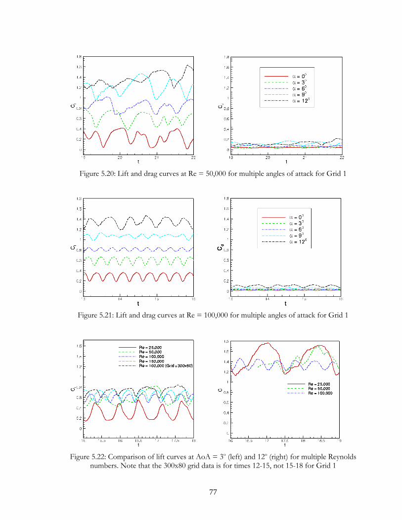
77
Figure 5.20: Lift and drag curves at Re = 50,000 for multiple angles of attack for Grid 1
Figure 5.21: Lift and drag curves at Re = 100,000 for multiple angles of attack for Grid 1
Figure 5.22: Comparison of lift curves at AoA = 3o (left) and 12o (right) for multiple Reynolds
numbers. Note that the 300x80 grid data is for times 12-15, not 15-18 for Grid 1

78
The results on the higher resolution grid 2 at a Reynolds number of 25,000 depicted
in figure 5.23 is consistent with the results obtained from grid 1. The lift behavior has
become increasingly irregular at higher angles of attack. This also holds for grid 3 which is
shows in figure 5.24.
At Re = 50,000 similar behavior is shown by grid 2 and grid 3 in comparison with
the results from grid 1. The results for Re = 50,000 from grid 2 and grid 3 are depicted in
figures 5.25 and 5.26.
Figure 5.23: Lift and drag curves at Re = 25,000 for multiple angles of attack for grid 2
Figure 5.24: Lift and drag curves at Re = 25,000 for multiple angles of attack for grid 3

79
Figure 5.25: Lift and drag curves at Re = 50,000 for multiple angles of attack for grid 2
Figure 5.26: Lift and drag curves at Re = 50,000 for multiple angles of attack for grid 3
5.7 Variation of lift with different grids
As all the computations for the non-oscillatory cases have been done using the three
grids as mentioned above, this section discusses the changes in the pattern of Cl curves with
different grids. The plots for Re = 25,000 are shown in figures from 5.27 to 5.31. At an angle
of attack of 00 for Re = 25,000 the variation of Cl is not large between the three grids but at

80
30 grid 3 shows higher lift compared to grid 1 and grid 2. For higher angles of attack the lift
behavior becomes irregular and no definite deviation was seen.
The corresponding lift plots for Re = 50,000 are shown in figures 5.32 to 5.36. At
lower angles of attack grid 3 was giving higher lift but at higher angles of attack the pattern
became irregular and no definite deviation in lift behavior was seen. The increment in the lift
shown by grid 3 at low angles of attack might be because the greater extent of this grid away
from the airfoil captures more vortices in the vicinity of the airfoil.
Figure 5.27: Cl and Cd plots for different grids for Re = 25,000 and AoA=00
Figure 5.28: Cl and Cd plots for different grids for Re = 25,000 and AoA=30

81
Figure 5.29: Cl and Cd plots for different grids for Re = 25,000 and AoA=60
Figure 5.30: Cl and Cd plots for different grids for Re = 25,000 and AoA=90
Figure 5.31: Cl and Cd plots for different grids for Re = 25,000 and AoA=120

82
Figure 5.32: Cl and Cd plots for different grids for Re = 50,000 and AoA=00
Figure 5.33: Cl and Cd plots for different grids for Re = 50,000 and AoA=30
Figure 5.34: Cl and Cd plots for different grids for Re = 50,000 and AoA=60

83
Figure 5.35: Cl and Cd plots for different grids for Re = 50,000 and AoA=90
Figure 5.36: Cl and Cd plots for different grids for Re = 50,000 and AoA=120

84
5.8 Vorticity distribution in comparison with lift and pressure plots for grid 1
For further illustration of the varying lift/drag behaviors the vorticity distribution
about the airfoils and coefficient of pressure distribution on the lower and upper surfaces are
presented at five points on a selected cycle for three Reynolds numbers at two angles of
attack in figures 5.37 – 5.42. At Re=25,000, both angles exhibit a large region of separation
defined by a vortex streak. At 3o, the streak extends almost to the trailing edge, at which
point it spins off distinct vortices, one with each oscillation of the lift curve. As an upper
vortex approaches the trailing edge, a counter-rotating vortex drawn from the lower surface
emerges at the trailing edge. At the point of maximum lift, this counter-vortex has just
detached from the trailing edge, after which a weak vortex pair trails off into the wake. The
decrease in the lift curves appears to correlate with the growth of the next upper surface
vortex, with the minimum lift occurring with the detachment of the upper vortex and during
the growth of the lower vortex. Self-evidently, the periodicity of this vortex development
process is the same as the lift curve oscillation. Increasing the angle of attack appears to
shorten the vortex streak and move the vortex generation point upstream, approaching the
midpoint of the chord for AoA=12o. While the frequency of oscillation has decreased, a
single vortex pair is again generated in each period. The vortices are notably stronger than
those at the lower angle of attack, consistent with the larger variation in lift values. The
upper vortex again appears to induce a counter vortex at the trailing edge, although at the
point of maximum lift this counter vortex is far off the trailing edge. Rather, the maximum
lift in this case appears to correlate with the stretching of the vortex streak and the
generation of a secondary counter vortex on the upper surface. This secondary counter

85
vortex helps separate the two upper surface vortices that exist as the lift declines towards the
minimum, although it does not persist as a coherent feature at the minimum lift point.
The pressure curves reflect the vortex activity. The vortex-free separation region is
clearly visible in the relative flat region on the upper surface extending from x/c=0.4–0.7 for
AoA=3o and 0.25–0.5 for 12o. Beyond this, the variable region on the upper surface
corresponds with the vortex-dominated region, with distinctly lower pressures as the lift is
increasing through the lift maximum and higher pressures as the lift decreases to the lift
minimum. The trailing edge shows large pressure variation, with very low pressures on both
surfaces near the minimum and very high pressures at the point of maximum lift. High lift
regions for both angles appear to be characterized by higher pressures on the lower surface
and lower pressures on the upper surface, while the converse is true for low lift. The
variation is more pronounced on the trailing half of the airfoil for both surfaces, even
though vortex activity is largely confined to the upper surface. At Re=50,000, fundamentally
different vortex patterns emerge. The vortex streak defining the separation region is now a
chain of vortices and the separation region itself is markedly thinner. At 3o, the vortex chain
extends to near the trailing edge, with the final vortex in the chain again pairing with a
counter vortex at the trailing edge to form a vortex pair downstream. The decrease in lift
appears to correlate with the generation of the counter vortex and the disruption of the
upper surface vortex chain. The point of maximum lift is well after the vortex pair separates
from the trailing edge. At 12o, the vortex chain is shorter, not extending past the midpoint of
the airfoil. The counter vortex generation on the trailing edge occurs despite the upper
vortices quickly drifting away from the upper surface. However, these two vortices do form
a vortex pair beyond the trailing edge. The irregularities in the lift curve at 12o suggest that

86
this pattern may vary significantly in detail from oscillation to oscillation; still, there appears
to be generally a single vortex pair generated in each oscillation.
The vortex chain region is evident in the pressure curves as a more regular and more
rapid oscillation in the upper surface pressure on top of a general increase in the mean
pressure downstream. The region extends over x/c=0.4–0.75, at which point the pressure
curves then take on the behavior of the vortex region seen in the Re=25,000 cases. A similar
vortex chain region is evident in the 12o between x/c=0.2-0.4, again followed by a vortex
region. At 3o, the lower surface pressure curve and the trailing edge behavior is similar to
that at Re=25,000; at 12o, the variability in these region is much less than that at the lower
Reynolds number, although the irregularity of the lift curve cautions against generalization.
At Re=100,000 the 3o vortex and pressure distributions are similar to those at Re=50,000,
despite the regularity of the oscillation at Re=100,000. In this case, the pressure curve
suggests that the vortex chain region extends from x/c=0.45 to nearly the trailing edge, with
no distinct vortex region. The 12o upper surface results are more similar to the 3o than the
12o results at Re = 50,000, with a long vortex chain region (0.2 – 0.7) followed by a vortex
region. The lower surface, however, shows smaller pressure variations as with the
Re=50,000, AoA=12o case. The separation region is again thin as with Re=50,000.
Figures for three different Reynolds numbers and remaining angles of attack are
presented in appendix A3.
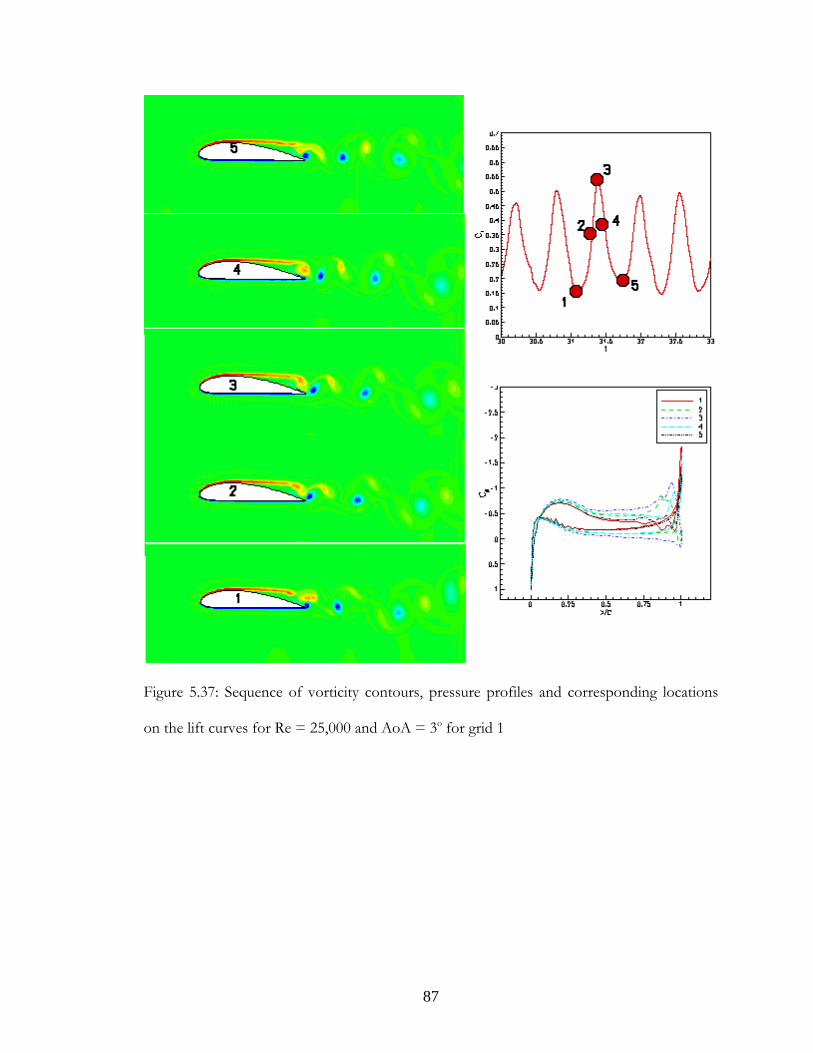
87
Figure 5.37: Sequence of vorticity contours, pressure profiles and corresponding locations
on the lift curves for Re = 25,000 and AoA = 3o for grid 1

88
Figure 5.38: Sequence of vorticity contours, pressure profiles and corresponding locations
on the lift curves for Re = 25,000 and AoA = 12o for grid 1

89
Figure 5.39: Sequence of vorticity contours, pressure profiles and corresponding locations
on the lift curves for Re = 50,000 and AoA = 3o for grid 1

90
Figure 5.40: Sequence of vorticity contours, pressure profiles and corresponding locations
on the lift curves for Re = 50,000 and AoA = 12o for grid 1

91
Figure 5.41: Sequence of vorticity contours, pressure profiles and corresponding locations
on the lift curves for Re = 100,000 and AoA = 3o for grid 1

92
Figure 5.42: Sequence of vorticity contours, pressure profiles and corresponding locations
on the lift curves for Re = 100,000 and AoA = 12o for grid 1

93
5.9 Vorticity distribution for grid 2 and grid 3
Vorticity distribution in comparison with lift and pressure curves at Reynolds
number of 25,000 and angles of attack 30 and 120 for grid 2 and grid 3 are presented in
figures 5.43-5.46. At 30 angle of attack grid 3 was showing stronger vortices which is also
evident from the lift curves but at 120 grid 2 was showing stronger vortices when compared
to grid 1 and grid 3. All the other characteristics such as formation vortex streaks and break
down of vortices as shown by grid 1 is also evident from grid 2 and grid 3 at corresponding
parameters of Reynolds number and angle of attack. Vorticity plots for Re = 50,000 can be
seen in appendix A3.

94
Figure 5.43: Sequence of vorticity contours, pressure profiles and corresponding locations
on the lift curves for Re = 25,000 and AoA = 3o for grid 2

95
Figure 5.44: Sequence of vorticity contours, pressure profiles and corresponding locations
on the lift curves for Re = 25,000 and AoA = 3o for grid 3

96
Figure 5.45: Sequence of vorticity contours, pressure profiles and corresponding locations
on the lift curves for Re = 25,000 and AoA = 12o for grid 2

97
Figure 5.46: Sequence of vorticity contours, pressure profiles and corresponding locations
on the lift curves for Re = 25,000 and AoA = 12o for grid 3

98
5.10 Summary of 155x80 grid data
This section presents a brief summary of the lift data obtained from the 155x80 grid.
Varation of Cl with angle of attack is shown in figure 5.47, which shows the increment in the
lift in the increase in Reynolds number at different angles of attack. The quasi-periodic
behavior of lift curves at Re = 50,000 posed some problem in the lift calculation, therefore
the lift data at this Reynolds number should be viewed with some uncertainty. Variation of
Cd with angle of attack is shown in figure 5.48 which clearly shows the decrease in drag with
the increase in Reynolds number. Frequency variation with angle of attack for different
Reynolds numbers is shown in figure 5.49, but as already said given the quasi-periodic
behavior of the lift curves at Re = 50,000 this data should be viewed with some uncertainty.
Drag polars at three different Reynolds numbers are presented in figure 5.50.
AOA
Cl
0 2 4 6 8 10 120
0.5
1
1.5
Re = 25,000Re = 50,000Re = 100,000
Figure 5.47: Variation of Cl with angle of attack at three different Reynolds numbers

99
AOA
Cd
0 2 4 6 8 10 120
0.05
0.1
0.15
0.2
0.25
0.3
Re = 25,000Re = 50,000Re = 100,000
Figure 5.48: Variation of Cd with angle of attack at three different Reynolds numbers
AOA
f
0 2 4 6 8 10 12
1
1.5
2
2.5
3 Re = 25,000Re = 50,000Re = 100,000
Figure 5.49: Variation of f with angle of attack at three different Reynolds numbers

100
Cd
Cl
0 0.05 0.1 0.15 0.2 0.25 0.30
0.5
1
1.5
Re = 25,000Re = 50,000Re = 100,000
Figure 5.50: Drag polar at three different Reynolds numbers

101
__________ CHAPTER
6 __________
CASE SETUP AND RESULTS FOR OSCILLATORY CASE
The last chapter dealt with setup details and results obtained through non-oscillating
surface cases; this chapter examines some preliminary cases where the surface of the airfoil
oscillates according to a given frequency. Two cases were considered for this purpose and
the results obtained through numerical simulations are compared to the experimental results.
Both of them show a drastic decrease in the separation.

102
6.1 Morphing Wing
The flow control approach described in this research is active flow control using a
morphing wing. It can be best described as a wing which has an internal actuator mounted in
it which oscillates depending upon the input frequency. Ideally, this frequency is the one that
would minimize separation. Sensors can be used to complete the feed-back loop. The
primary wing considered for this study is NACA 4415 airfoil because it has sufficient
thickness to accommodate the flow control mechanism. The basic working mechanism of
this wing is described below.
Figure 6.1: Computational assumption for the oscillatory control approach
Figure 6.1 shows the baseline airfoil which is NACA 4415 and minimum and maximum
positions for the oscillatory surface (A represents the maximum position and B represents
minimum position). As already stated this oscillatory surface extends from 20% to 80% of
chord length. The actuator, which is mounted internally into the airfoil, does the work of
oscillation of the surface. For the initial implementation from the numerical simulations
point of view it has been assumed that the position A represents NACA 4416 airfoil and
position B represents NACA 4414 airfoil. The exact shapes of the deforming airfoil are not
NACA 4415
B
A
Actuator
103
known, but NACA 4414 and NACA 4416 should reasonable resemble to the actual
experiments. Hence for a given energy input the surface oscillated been NACA 4414 and
NACA 4416 at a given frequency, and when there is no oscillation it attains the shape of
NACA 4415. The two specific cases considered for morphing are Reynolds number of
25,000 and angle of attack of 30 and 90.
6.2 Case Setup
For the oscillatory case simulations the grid setup established for static case
simulations have been used except for the airfoil grid which is further divided into an
oscillatory zone and non-oscillatory zone. Further sections deal with the implementation of
the morphing cases into GHOST.
6.2.1 Implementation of Morphing into GHOST
Implementing morphing in the current code has been done using the following
preliminary approach.
For all the preliminary cases it has been assumed that the airfoil vibrates up and
down, changing its shape in the middle portion of the upper surface from 20% of chord
length to the 80% of chord length, with leading and trailing edges being fixed. As mentioned
earlier, to simplify the implementation in the computational model it has been assumed that
the airfoil attains the shape of NACA 4416 when the actuator is at its maximum position and
attains the shape of NACA 4414 when the actuator is at is minimum position. An
overlapping grid for the morphing region between 20% and 80% of the chord length on the
upper surface is moved at the frequencies used in the experimental results. Figure 6.2 shows
the morphing region along with the non-morphing region. All the grid points in the
morphing region are moved with predetermined velocities based on the particular

104
experiment being examined. Figure 6.3 shows the maximum and minimum displacement
positions for the morphing region along with the intermediate positions. The movement of
the morphing surface is limited to the y-direction only, so the morphing surface has zero u
velocity. This reasonable approximation is used to simplify the modeling, requiring the input
of only v velocity values for each grid point as illustrated in figure 6.3.
During this motion the volume of each control volume element in the morphing
region is conserved. Figure 6.4 shows the shape of the control volume before and after the
velocity input in two stages (stage 1 and stage 2). In the morphing region, for a given i each
i,j-gridpoint is given the same dy value (dy1 and dy2 remain the same for each pair of grid
points along their respective j direction). As such, the values of ∆y and ∆x are unchanged,
leaving the area constant. Therefore the effective area of the control volume at stage 1 is
equal to the area of the control volume at stage 2.
V
U
Stationary Grid
Moving Grid
Figure 6.2: Morphing grid and Stationary grid
along with U and V velocity directions

105
Figure 6.3: Morphing part at its maximum and minimum displacements along with the intermediate positions in the CFD run.
Figure 6.4: Control volume before and after the displacement input (v velocity) for two grid points.
Intermediate positions
Morphing Part at its maximum and minimum Displacements
v U = 0
x
y
-0.1 0 0.1 0.2 0.3 0.40.1
0.2
0.3
0.4
0.5
0.6
x
y
-0.055 -0.05 -0.045 -0.04 -0.035
0.265
0.27
∆y ∆x
dy2dy1
Control Volume at stage 1 Control Volume at stage 2

106
6.2.2 Calculation of u and v velocities for the morphing
The two cases considered for numerical simulations are at a Reynolds number of
25,000 at 30 and 90 angles of attack. For the first case at Reynolds number of 25,000 and
angle of attack of 00 experiments were conducted with an actuator frequency of 15Hz. In
order to input that frequency into the CFD code this frequency has been converted to u and
v velocities for the each and every grid point on the morphing zone. This calculation is done
as follows.
5
25
3
10*6.1/)203.0*(000,25Re
203.0''8/10*6.1
/18.1
−
−
===
===
=
uulml
smmkg
µρ
υ
ρ
⇒ smu /97.1= sulT 103.097.1/203.0/ === sec0666.015/115 ==⇒= THzf Therefore non dimensional time for CFD code = 0.0666 / 0.103 = 0.646601 Time step in the CFD code = 0.0001000931733 Number of grid changes required for one cycle (0.646601) = 0.646601/0.0001000931733
= 6460
These 6460 grid changes are what is necessary for the airfoil to smoothly move from
the NACA 4414 to NACA 4416 and then back to NACA 4414. It was impractical to input
this many grid changes into the CFD code, hence we have minimized the number of grid
changes to 68 and made the code to run for 95 time steps at each grid thereby making 68*95
= 6460. But for each increment in the time step each grid point on the morphing zone has
been given the same v velocity which has been calculated as shown below.
(For air at room temperature) (6.1)(6.2)(6.3)
(6.4)
(6.5)
(6.6)
(6.7)
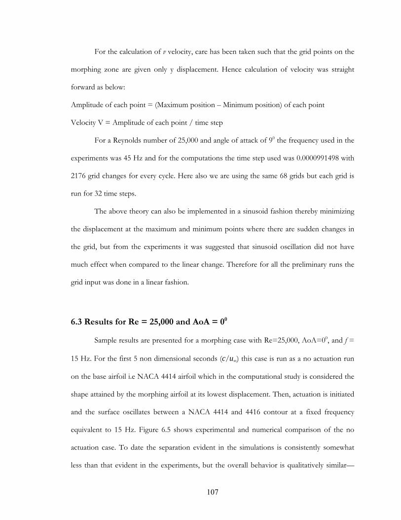
107
For the calculation of v velocity, care has been taken such that the grid points on the
morphing zone are given only y displacement. Hence calculation of velocity was straight
forward as below:
Amplitude of each point = (Maximum position – Minimum position) of each point
Velocity V = Amplitude of each point / time step
For a Reynolds number of 25,000 and angle of attack of 90 the frequency used in the
experiments was 45 Hz and for the computations the time step used was 0.0000991498 with
2176 grid changes for every cycle. Here also we are using the same 68 grids but each grid is
run for 32 time steps.
The above theory can also be implemented in a sinusoid fashion thereby minimizing
the displacement at the maximum and minimum points where there are sudden changes in
the grid, but from the experiments it was suggested that sinusoid oscillation did not have
much effect when compared to the linear change. Therefore for all the preliminary runs the
grid input was done in a linear fashion.
6.3 Results for Re = 25,000 and AoA = 00
Sample results are presented for a morphing case with Re=25,000, AoA=00, and f =
15 Hz. For the first 5 non dimensional seconds (c/u∞) this case is run as a no actuation run
on the base airfoil i.e NACA 4414 airfoil which in the computational study is considered the
shape attained by the morphing airfoil at its lowest displacement. Then, actuation is initiated
and the surface oscillates between a NACA 4414 and 4416 contour at a fixed frequency
equivalent to 15 Hz. Figure 6.5 shows experimental and numerical comparison of the no
actuation case. To date the separation evident in the simulations is consistently somewhat
less than that evident in the experiments, but the overall behavior is qualitatively similar—

108
some of the discrepancy is possibly due to the wall effects discussed in chapter 5. When
morphing is implemented on this same configuration a sizeable decrease in the separation
was seen, which is depicted in figure 6.6. The separation region for the morphing case in the
simulations is dominated by the formation of vortices. The formation and breakdown of
these vortices is clearly seen in the figure 6.7. Figure 6.8 compares the lift and drag curves
for the actuation and no actuation case. The no actuation case yields an oscillatory lift
behavior with a period of 0.33 in dimensionless time (c/u∞). The actuated case also exhibits
oscillatory behavior but with a period of 0.66. The shapes of the curves are also distinctly
different, shifting from sharp peaks and wide troughs to sharp troughs and wide peaks. The
average lift of the actuator case is also increased considerably when compared to the no
actuation case (figure 6.8). The increment in the lift is also supported by the decrease in the
drag value of the actuator case.
a) Experiment from Munday et al [26]
b) Computation
Figure 6.5: Instantaneous stream line plot for no actuation case for Re = 25,000 and
AoA = 00

109
Note that the current numerical methods result in occasional sharp peaks in lift and
drag—at present it is assumed that these peaks are formed because of the sudden changes in
the airfoil shape but it can be investigated further with the availability of experimental data.
a) Experiment from Munday et al [26]
b) Computation
Figure 6.6: Instantaneous stream line plots for actuation at f = 15 Hz for Re = 25,000 and
AoA = 00
Figure 6.7: Instantaneous vorticity plots at different instances for no actuation and actuation
case Re = 25,000, AoA = 00
a) No Actuation b) Actuation at f = 15hz

110
Figure 6.8: Lift and Drag Coefficient curves of the actuation case at f = 15 Hz in comparison
with the unactuated cases for Re = 25,000 and AoA = 00
6.4 Results for Re = 25,000 and AoA = 90
As done with the previous case this case is also run as a no actuation run on the base
airfoil i.e NACA 4414 airfoil for for 5.75 non-dimensional seconds. Then the actuation is
applied at a frequency of 45 Hz (this frequency is again selected to match the available
experiments) to oscillate the portion of the wing between the profiles of NACA 4416 and
NACA 4414. Figure 6.9 shows the experimental and numerical instantaneous stream line
plot for the no actuation case, where a large separation region is observed. Separation is
almost similar for both experiments and simulations except that the formation of vortices is
seen in the simulations. When the actuation at a rate of 45 Hz is applied, a radical decrease in
separation in seen in experiments but in simulations reduction in separation is somewhat
less. The separation region in simulations is dominated by the formation of vortices which is
not evident from experiments. Figure 6.10 shows the instantaneous vorticity plots for no

111
actuation and actuation cases. From this (figure 6.10) the formation and break-down of
vortices in the separation region is clearly seen. The corresponding lift and drag plots are
presented in figure 6.11 which shows a regular behavior being observed in actuation case but
with some heavy noise. This noise is not shown in vorticity plots but is evident from lift
plots. Figure 6.11 also shows that the drag is reduced considerably increasing the lift to drag
ratio. Unlike the previous case (Re = 25,000 and AoA = 00) where oscillation frequency is
similar to the periodicity of the lift curves, in this case the lift periodicity which is 0.9 in
dimensionless time dominates the oscillation frequency.
a) Experiment from Munday et al [26]
b) Computation
Figure 6.9: Instantaneous stream line plot for no actuation case for Re = 25,000 and AoA = 00

112
a) Experiment from Munday et al [26]
b) Computation
Figure 6.10: Instantaneous stream line plot for at f = 45 Hz for Re = 25,000 and AoA = 90
Figure 6.11: Instantaneous vorticity plots at different instances for non actuation case
actuation case Re = 25,000, AoA = 90
a) No Actuation b) Actuation at f = 45 Hz

113
Figure 6.12: Lift and Drag Coefficient curves for actuation case at f = 45 Hz in comparison
with the unactuated case for Re = 25,000 and AoA = 90
6.5 Analysis of lift data
Further investigation has been made into the reason behind the noise seen in the lift
data from the above two mentioned cases. Two approaches have been selected for this
purpose.
1. Obtaining lift through downstream momentum calculation
2. Doing the morphing run with actual grid change at every time step (Expensive
process)
For Re = 25,000 and AoA = 90 lift data has been obtained through integrating
downstream momentum and is compared to the actual lift data obtained from pressure data.
The comparison can be seen from figure 6.13. Lift obtained through downstream
momentum fairly follows the lift obtained through pressure data without any noise. This
clearly demonstrates that the overall picture obtained through pressure data fairly coincides
with the physics of the flow.

114
Another approach involved changing the grid at every time step (which is the correct
way of doing the morphing run) unlike the sudden impulse approach used in this thesis. The
result obtained through this approach in comparison with the grid change for 95 time steps
can be seen in figure 6.14. Figure 6.14 clearly demonstrates that changing the grid at every
time step would completely eliminate the noise and it follows the mean path of the lift curve
obtained by changing grid for every 95 time steps. However, this is a much more expensive
process for doing the morphing run as currently implemented and the mid-range pressure
curve and the other two methods seem largely coincident. For now, it can be concluded that
changing grid for every 95 time steps probably give qualitatively good results.
Figure 6.13: Comparison of Cl obtained through pressure data and downstream momentum
calculation for Re = 25,000, AoA = 90 at f = 45 Hz

115
t
Cl
5.18 5.185 5.19 5.195 5.2 5.205 5.21 5.215 5.22-0.2
-0.15
-0.1
-0.05
0
0.05
0.1
Grid change at each time stepGrid change after 95 Steps
Figure 6.14: Comparison of Cl obtained through grid change for 95 time steps and at each
time step for Re = 25,000, AoA = 00 at f = 15 Hz

116
__________ CHAPTER
7 __________
CONCLUSIONS AND FUTURE WORK
7.1 Conclusions
An oscillatory flow control mechanism is successfully implemented in the numerical
simulations and the results showed a great improvement in the lift to drag ratio. Before
proceeding to oscillatory flow control a wide number of numerical simulations were
performed for non oscillatory control cases and these results are in qualitative agreement
with the experimental results. Preliminary studies for time step and transition were
performed and an effective time step was established for the simulations in the present
studies.

117
The unsteady flow pattern made the choice for an airfoil grid a difficult one.
Numerous simulations were performed with different grid sizes and comparison of the
frequencies obtained through the lift curves was made which lead to an alternate analysis
based on cylinder runs. These cylinder simulations were performed by replacing the airfoil
grid with equivalent cylinder grid and comparing the Strouhal number with the experimental
results. These cylinder simulations decreased the vast number of grid choices to three grids.
Further studies on those three grids still showed some differences in the lift behavior but it
was justified by doing all the simulations with all three grids.
The variation between the results obtained from three different airfoil grids was seen
in lift curves but not shown greatly in vorticity behavior. The difference in the results was
insignificant at a zero angle of attack. At 30 and Reynolds number of 25,000 there was a great
difference in lift curves. For higher angles of attack there was no clear pattern shown by the
three different grids and hence it was difficult to judge which grid yielded the best result.
From the computations performed in the current research for non-oscillatory cases,
potentially useful trends were observed from the current data. At Re=25,000, the flow is
characterized by a vortex streak, a thick separation region, and a lift curve with sharp peaks
and broader valleys (although this is less pronounced at higher angles of attack). At higher
Reynolds numbers, the vortex streak is replaced by a vortex chain with a distinctly different
pressure distribution, the separation region thins, and the lift curve has broader peaks and
sharp troughs. Increasing angle of attack shortens the length of the vortex streak or chain
region in favor of a larger region with distinct vortices, in some cases with additional counter
vortices. Also, the pressure curves become less variable on the lower surface at higher angles
of attack for higher Reynolds numbers. The thin separation region at higher Reynolds
numbers correlates with the lower magnitude of the drag increase with angle of attack.

118
Conveniently, the nature of the vortex behavior appears to be reflected in the pressure
curves, a useful point of comparison to experimental data.
The oscillatory flow control approach used in the current research decreased the
separation. Two preliminary simulations performed at Reynolds number of 25,000 and
angles of attack of 30 and 90 showed qualitatively similar behavior as that of experiments.
The lift values obtained through simulations showed some peculiar behavior with drastic
changes in the lift but by calculating averaged lift in each interval these variations were
largely eliminated for the 00 case but could not be eliminated for 90 case. The proper
correction is to change the grid at every time step as demonstrated but at this point that
exercise is computationally expensive.
7.2 Future Work
Preliminary experimental data from the 24x24 inch test section will be available in
the near future, at which point the no actuation results should be reviewed with the
experiments therefore completing the parameter study of the no actuation cases. More
simulations need to be performed for oscillatory cases and effect of oscillatory flow control
at higher Reynolds numbers should be studied. It has to be seen whether the lift behavior
shown by oscillatory cases holds well or not in the experiments.

119
__________ APPENDIX
__________
A1. SST Turbulence Model (Menter, 1994)
Menter’s SST model is based on a mix of two equation ωκ − and εκ − turbulence models
using a blending function FB1 B. The model can be written as
κ -equation:
( ) ⎟⎟⎠
⎞⎜⎜⎝
⎛
∂∂
+∂∂
+−=∂
∂+
∂∂
jtk
jk
j
j
xxP
xu
tκµσµρωκ
κρρκ 09.0 (A1)
ω-equation:
( ) ( )jjj
tj
ktj
j
xxF
xxPc
xu
t ∂∂
∂∂
−+⎟⎟⎠
⎞⎜⎜⎝
⎛
∂∂
+∂∂
+−=∂
∂+
∂∂ ωκ
ωσρωµσµβρω
υωρρω
ωω112 21
2 (A2)
The constants, c, β, ,, ωκ σσ and are given by the following general expression
2111 )1( φφφ FF −+= (A3)
where φ represents any one of these constants; 1φ represents any constant in the
ωκ − model; 2φ represents the corresponding constant in the εκ − model. These
constants are defined as

120
Set 1 ( ωκ − ):
85.01 =κσ , 5.01 =ωσ , 075.01 =β , 553.01 =c (A4)
Set 2 ( εκ − ):
0.12 =κσ , 856.02 =ωσ , 0828.02 =β , 44.02 =c (A5)
The Production term is given as
j
iij x
uP
∂∂
= τκ (A6)
where
ijijk
k
i
j
j
itij x
uxu
xu
ρκδδµτ32
32
−⎥⎥⎦
⎤
⎢⎢⎣
⎡
∂∂
−∂
∂+
∂∂
= (A7)
The blending function FB1 B is defined as
( )411 argtanh=F (A8)
with
⎪⎭
⎪⎬⎫
⎪⎩
⎪⎨⎧
⎥⎦
⎤⎢⎣
⎡= 2
221
4;500;
09.0maxminarg
dCDdd κω
ω κρσων
ωκ (A9)
where d is the distance to the closest wall and κωCD is the positive portion of the cross-
diffusion term in Eq. (A2).
⎥⎥⎦
⎤
⎢⎢⎣
⎡
∂∂
∂∂
= −202 10;12max
jj xxCD ωκ
ωρσωκω (A10)
The kinematic eddy viscosity is defined as
( )21
1
;max Faa
t Ω=
ωκ
ν (A11)
where Ω is the magnitude of vorticity and 1a = 0.31. The function F B2 B is given by
B ( )222 argtanh=F B(A12)B
with
⎥⎦
⎤⎢⎣
⎡=
ων
ωκ
22500;
09.02maxarg
dd (A13)

121
A2. Boundary Conditions in the GHOST
This section deals with the boundary conditions which were used in this thesis and
are available in the codes explained in chapter 3. All the boundary conditions are described
using the code snippets, and the following constants were used in those code snippets.
1. Free stream velocity, uref = 1.
2. Turbulent Kinetic Energy, tkref = (uref * 0.01)**2
3. Viscosity , viscos = 1./Re.
4. Turbulent Viscosity, tvisref = 1. * viscos
5. Density, densit = 1.
6. Cµ, cmu = 0.09
7. edref_ke = cmu * tkref ** 2/ tvisref * densit
8. u represents the velocity in x direction
9. v represents the velocity in y direction
10. p represents the pressure
11. imodel designates the turbulence model
1.0 Inlet Boundary Condition
Unless required to input the velocity profile we use the boundary condition as shown
in the code present in this section. Pressure at the inlet boundary is made equal to the
pressure in the adjacent cells of the boundary. When SST turbulence model is to be used,
which is designated by setting imodel in the code snippet is to 1 and the turbulent kinetic
energy and eddy viscosity values are set to the reference values.
v (i, j) = 0.
u (i, j) = uref
p (i, j) = p (i_n, j_n)

122
IF (imodel == 1) THEN
tk (i, j) = tkref
ed (i, j) = edref_ke
END IF
2.0 Outflow Boundary Condition
For this boundary condition velocity and pressure values at the boundary are made
equal to the values in the adjacent cells of the boundary
v (i, j) = v (i_n, j_n)
u (i, j) = u (i_n, j_n)
p (i, j) = p (i_n, j_n)
3.0 Wall Boundary Condition
Code snippet for the wall boundary condition is as follows
v (i, j) = 0.
u (i, j) = 0.
p (i, j) = p (i_n, j_n)
IF (imodel == 1) THEN
tk (i, j) = 0.
ed (i, j) = 0.
END IF
4.0 Block Boundary Condition
This boundary condition is used to specify the zone where there is no computation is
necessary. For the present research we used this boundary condition for the airfoil inner
part.
v (i, j) = 0.
u (i, j) = 0.
p (i, j) = 0.

123
A3. Vorticity distribution in comparison with lift and pressure plots for various angles of attacks and Reynolds numbers for different grids Vorticity plots in comparison with lift and pressure variation are presented in this
section for some of the Reynolds numbers and angles of attack in addition to the plots
presented in chapter 5. Most of the plots presented in this section are for the 155x80 grid
but some of the plots for the other two grids are also included in this section. Grid 3 at Re =
25,000 and AoA = 30 showed somewhat stronger vorticity behavior when compared to
other two grids. This stronger vorticity behavior is reflected in higher lift behavior.
Figure A3.1 : Sequence of vorticity contours, pressure profiles and corresponding locations
on the lift curves for Re = 25,000 and AoA = 0o for Grid 1

124
Figure A3.2 : Sequence of vorticity contours, pressure profiles and corresponding locations
on the lift curves for Re = 25,000 and AoA = 6o for Grid 1
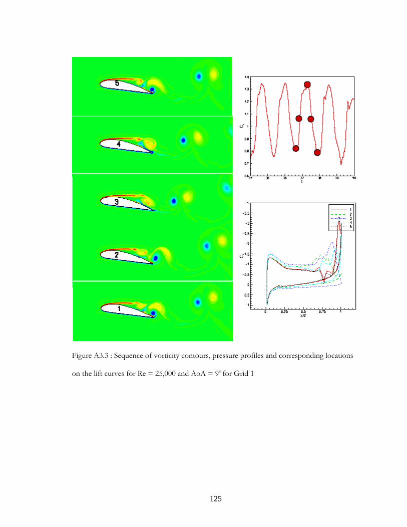
125
Figure A3.3 : Sequence of vorticity contours, pressure profiles and corresponding locations
on the lift curves for Re = 25,000 and AoA = 9o for Grid 1

126
Figure A3.4 : Sequence of vorticity contours, pressure profiles and corresponding locations
on the lift curves for Re = 50,000 and AoA = 0o for Grid 1

127
Figure A3.5 : Sequence of vorticity contours, pressure profiles and corresponding locations
on the lift curves for Re = 50,000 and AoA = 6o for Grid 1

128
Figure A3.6 : Sequence of vorticity contours, pressure profiles and corresponding locations
on the lift curves for Re = 50,000 and AoA = 9o for Grid 1

129
Figure A3.7 : Sequence of vorticity contours, pressure profiles and corresponding locations
on the lift curves for Re = 100,000 and AoA = 0o for Grid 1

130
Figure A3.8 : Sequence of vorticity contours, pressure profiles and corresponding locations
on the lift curves for Re = 100,000 and AoA = 6o for Grid 1
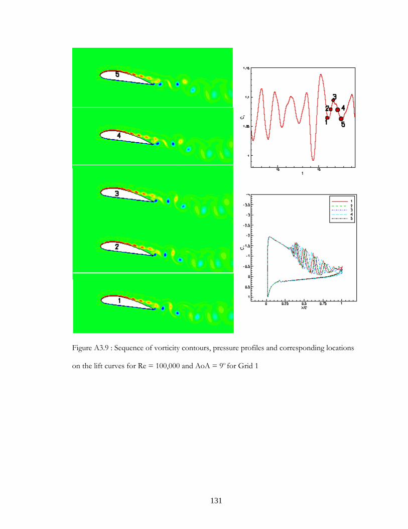
131
Figure A3.9 : Sequence of vorticity contours, pressure profiles and corresponding locations
on the lift curves for Re = 100,000 and AoA = 9o for Grid 1

132
Figure A3.10 : Sequence of vorticity contours, pressure profiles and corresponding locations
on the lift curves for Re = 50,000 and AoA = 3o for grid 2

133
REFERENCES
1. Thomas J. Mueller, James D. DeLaurie “ Aerodynamics of Small Vehicles” Annual
Review of Fluid Mechanics, 2003, pp 89 – 111
2. Gad-el-Hak M, “ Micro-Air-Vehicles: Can They be Controlled Better ?”, Journal of
Aircraft, Vol 38, 2001, pp 419 – 429
3. Mark Drela, “ Low-Reynolds-Number Airfoil Design for the M.I.T Daedalus
Prototype: A Case Study”, Journal of Aircraft, vol. 25, 1998, pp 724-732
4. Thomas J. Mueller. “Aerodynamic Measurements of low Reynolds Number for
Fixed wing Micro-Air Vehicles.” Presented at the RTO AVT/VKI special course on
Development and Operation of UAV’s for Military and Civil applications.
5. Rule, J.A. , Richard, R.E. , Clark, R.L., “ Design of and Aero Elastic Delta Wing
Model for Active Flutter Control” Journal of Guidance, Control, and Dynamics, 24,
n 5, 2001, pp 918-924
6. B. Thwaites, “Approximate Calculation of the Laminar Boundary Layer”,
Aeronautical Quarterly, Vol. 1, 1949, pp. 245-280
7. B. S. Stratford, “The Prediction of Separation of the Turbulent Boundary Layer”,
Journal of Fluid Mechanics, Vol. 5, 1959, pp. 1-16
8. N. Curle and S. Skan, “Approximate Methods for Predicting Properties of Laminar
Boundary Layers”, Aeronautical Quarterly, Vol. 8, 1957, pp. 257-268
9. M. Gad-el-Hak, “Control of Low-Speed Airfoil Aerodynamics”, AIAA Journal, Vol.
28, 1990, pp. 1537-1552

134
10. McCullough, G. B., and Gault, D.E., “ Examples of Three Representative Types of
Airfoil-Section Stall at Low Speed,” NACA TN-2502, Washington, DC, 1951
11. Meuller, T. J., and Burns, T.F., “Experimental Studies of the Eppler 61 Airfoil at
Low Reynolds Numbers,” AIAA Paper 82-0345, 1982.
12. Sunada, S., Sakaguchi, A., Kawachi, K., “Airfoil section characteristics at a low
Reynolds number.” ,Journal of fluids engineering, Transactions of the ASME, Vol.
119,1997, pp 129-135.
13. Pfenninger, W., and Vemuru, C. S., “ Design of Low Reynolds Number Airfoils: Part
I” Journal of Aircraft, Vol. 27,1990, pp 204-210
14. Selig, M. S., and Guglielmo, J., “High-Lift Low Reynolds Number Airfoil Design”
Journal of Aircraft, Vol. 34, 1997, pp 72-78
15. Truckenbrodt, E., “Ein einfaches Naherungsverfahren zum Berechnen der
laminaren reibungsschicht mit Absaugung,” Forschg. Ing.-Wes. Vol. 22, 1956, pp.
147-157.
16. Prandtl, L., “The Mechanics of Viscous Fluids,”Aedoynamic Theory, Vol. III, edited
by W.F. Durand, Springer, Berlin, 1935, pp.34-208
17. McLachlan, B.G., “Study of Circulation Control Airfoil with Leading/Trailing-Edge
Blowing,” Journal of Aircraft, Vol. 26, 1989, pp.817-821.
18. Mangalam, S. M., Bar-Sever, A., Zaman, K. B. M. Q., and Harvey, W. D.,
“Transition and Separation Control on a Low-Reynolds Number Airfoil,”
Proceedings of the International Conference on Aerodynamics of Low Reynolds
Numbers, Vol. I, Royal Aeronautical Society, London, 1986, pp. 10.1-10.19
19. Harvey, W.D., “Low-Reynolds Number Aerodynamics Research at NASA Langley
Research Center,” Proceedings of the International Conference on Aerodynamics at

135
Low Reynolds Numbers, Vol II, Royal Aeronautical Society, London, 1986, pp. 19.1-
19.49
20. Mehta, R. D., “ Effect of a Longitudinal Vortex on a Separated Turbulent Boundary
Layer,” AIAA Paper 85-0530, 1985
21. Rao, D. M., and Kariya, T. T., “Boundary-Layer Submerged Vortex Generators for
Separation Control—An Exploratory Study,” AIAA Paper 88-3546-CP, 1988.
22. Lissaman P.B.S, “Low-Reynolds-Number Airfoils” Annual Review of Fluid
Mechanics, 1983, pp 223-239.
23. Tani Itiro, “Low-speed Flows Involving Bubble Separations”, Progress in
Aeronautical Siences, Vol. 5, edited by D.Kuchenmann and L. H.G. Sterne,
Pergamon Press, New York, 1964, pp. 70-103.
24. Stanewsky, E., “Aerodynamic Benefits of Adaptive Wing Technology,” Aerospace
Sciences and Technology, 2000, pp 439-452
25. Jacob, J.D, “On the Fluid Dynamics of Adaptive Airfoils”, Proceedings of 1998
ASME International Mechanical Engineering Congress and Exposition, Anaheim,
CA, 1998 Nov 15-20
26. Munday, D., Jacob, J. D., “Active Control of Separation on a Wing with Conformal
Camber,” AIAA Paper 2001-0293, 2001
27. Munday, D., Jacob, J. D., Hauser, T., Huang, G., “Experimental and Numerical
Investigation of Aerodynamic Flow Control Using Oscillating Adaptive Surfaces,”
AIAA 2002-2837,2002
28. Ekaterinairs, J.A., Chandrasekhara, M.S., and Platzer, M.F. “Analysis of Low
Reynolds Number Airfoil Flows,” Journal of Aircraft, vol. 32, No. 3, 1995, pp. 627 –
630

136
29. Chen, K. K., and Thyson, N. A., “Extension of Emmons Spot Theory to Flows on
Blunt Bodies,” AIAA Journal, Vol. 9, No. 5, 1971, pp. 821 – 825
30. Tatineni, M., Zhong, X., “Numerical Simulation of Unsteady Low-Reynolds-
Number Separated Flows over Airfoils”, AIAA Journal, Vol. 38, pp 1295-1300
31. Shum Y. K., and Marsden D. J., “Separation Bubble Model for Low Reynolds
Number Airfoil Applications” Journal of Aircraft, vol. 31, No. 4, 1994, pp. 761-766
32. Pinkerton, T. L. and Moses, R. W., “A Feasibility Study to Control Airfoil Shape
Using THUNDER," NASA TM 4767, 1997.
33. Munday D. Jacob J. D., Huang G., “Active Flow Control of Separation on a Wing
with Oscillatory Camber” AIAA 2002-0413, 2002
34. Katam V., LeBeau, R. P., Jacob J.D., “Experimental and Computational
Investigation of a Modified NACA4415 in Low-Re Flows”, AIAA 2004-4972
35. Seifert, A. and Pack, L. G., “Active Flow Separation Control on Wall-Mounted
Hump at High Reynolds Numbers,” AIAA Journal, Vol. 40, No. 7, July 2002. pp
1364-1372
36. Seifert, A. and Pack, L.G., “Effects of Sweep on Active Separation Control at High
Reynolds Numbers”, Journal of Aircraft, Vol. 40, No.1,Jan-Feb 2003.pp 120-126
37. Seifert, A. and Pack, L.G., “Compressibility and Excitation Location Effects on High
Reynolds Numbers Active Separation Control,” Journal of Aircraft, Vol.40, No. 1,
Jan-Feb 2003. pp 110-120
38. http://cfdval2004.larc.nasa.gov
39. D. Greenblatt, N.W. Schaeffler, A.E. Washburn, K. Paschal, J. Harris & C. Yao
“Separation Control over a Wall-Mounted Hump (Wall-Mounted Glauert-Glas

137
Airfoil)” Presentation at CFD Validation of Synthetic Jets and Turbulent Separation
Control, Langley Research Center Workshop, Langley, VA, March 29-31,2004
40. D. Greenblatt, N.W. Schaeffler, A.E. Washburn, K. Paschal, J. Harris & C. Yao, “ A
Separation Control CFD Validation Test Case Part I: Baseline and Steady Suction,”
AIAA Paper 2004-2220, June-July 2004
41. Suzen, Y.B. and Huang, P.G., "Numerical Simulation of Wake Passing on Turbine
Cascades", AIAA-2003-1256, 2003.
42. Suzen, Y.B., Huang, P.G., Volino, R.J., Corke, T.C., Thomas, F.O., Huang, J., Lake,
J.P., and King, P.I., “A Comprehensive CFD Study of Transitional Flows In Low-
Pressure Turbines Under a Wide Range of Operation Conditions”, AIAA 2003-
3591, 2003.
43. Suzen, Y.B., and Huang, P.G., “Predictions of Separated and Transitional Boundary
Layers Under Low-Pressure Turbine Airfoil Conditions Using an Intermittency
Transport Equation”, Journal of Turbomachinery, Vol. 125, No.3, Jul. 2003, pp. 455-464.
44. Huang, L., Huang, P.G., LeBeau, R.P., Hauser, Th., “Numerical Study of Blowing
and Suction Control Mechanism on NACA0012 Airfoil”, Journal of Aircraft, Vol. 41,
2004, pp. 1005-1013.
45. Huang, L., Huang, P.G, LeBeau, R.P., and Hauser, Th., “Optimization of Blowing
and Suction Control on NACA 0012 Airfoil Using a Genetic Algorithm”, AIAA-
2004-0423, 2004.
46. Huang, L., LeBeau, R.P., and Hauser, Th., “Application of Genetic Algorithm to
Two-Jet Control System on NACA 0012 Airfoil”, Proceedings of the International
Conference on Computational Fluid Dynamics 3, Toronto, Canada, July 12-14, 2004.

138
47. Chen, H., Huang, P.G., and LeBeau, R.P., “Parallel 2D/3D Unsteady Incompressible
Viscous Flow Computations Using an Unstructured CFD Code”, Proceedings of the
International Conference on Computational Fluid Dynamics 3, Toronto, Canada,
July 12-14, 2004.
48. Chen, H., Huang, P.G., and LeBeau, R.P., “A Cell-Centered Pressure Based Method
for Two/Three-Dimensional Unstructured Incompressible Navier-Stokes Solver”,
AIAA-2005-0880, 2005.
49. Rhie, C. M. and Chow, W. L., “Numerical study of the turbulent flow past an airfoil
with tailing edge separation,” AIAA J., vol. 21, 1983, pp. 1525-1532.
50. F. R. Menter, “Two-Equation Eddy-Viscosity Turbulence Models For Engineering
Applications”, AIAA Journal, Vol. 32, No. 8, Aug. 1994, pp. 1598-1605
51. Y. Suzen, G. Huang, “Comprehensive Validation of an Intermittency Transport
Model for Transitional Low-Pressure Turbine Flows”, AIAA 2004-1121 42P
ndP
Aerospace Sciences Meeting and Exhibit, Jan.2004
52. Karypis, G. and Kumar, V., A software package for partitioning unstructured graphs,
partitioning meshes, and computing fill-reducing orderings of sparse matrices
version 4.0. TUhttp://www.cs.umn.edu/~karypisUT, 1998.
53. Zdravkovich M. M., “Flow Around Circular Cylinders”, Oxford University Press.
1997
54. James L. Thomas and M. D. Salas “Far-Field Boundary Conditions for Transonic
Lifting Solutions to the Euler Equations” AIAA Journal, Vol. 24, No.7 pp 1074-
1080.

139
VITA
Vamsidhar Reddy Katam was born in Hyderabad, India on 27th May 1981. He
obtained his undergraduate degree from J.N.T University, Hyderabad in May 2002 and
performed his graduate studies at University of Kentucky. He worked as a Research assistant
at University of Kentucky and presented his research work at national and international level
conferences.
Conferences
Katam, V., R.P. LeBeau, and J.D. Jacob, “Simulation of Separation Control on a Morphing
Wing with Conformal Camber” Accepted to 35th Fluid Dynamics Conference, Toronto,
Ontario, Canada, June 6-9, 2005.
Katam, V., R.P. LeBeau, and J.D. Jacob, “Separation Control Using a Wing with Oscillatory
Camber in Low-Re Flows”, 30th Annual Dayton-Cincinnati Aerospace Science Symposium,
Dayton, OH, March 8, 2005.
Katam, V., R.P. LeBeau, and J.D. Jacob, "Experimental and Computational Investigation of
a Modified NACA 4415 in Low-Re Flows," 22nd Applied Aerodynamics Conference and
Exhibit, AIAA 2004-4972 , August 2004.
Katam, V., H.Chen, L.Huang, V.Parimi, R.P.LeBeau and P.G.Huang, “Two-Dimensional
Simulation of Flow Over a Hump Model with Mentor’s SST Model,” CFD Validation of
Synthetic Jets and Turbulent Separation Control, Langley Research Center Workshop,
Langley, VA, March 29-31,2004
Katam, V., R.P. LeBeau, and J.D. Jacob, "Investigation of Low Reynolds Number Flows
over a Modified NACA 4415 Airfoil," 29th Annual Dayton-Cincinnati Aerospace Science
Symposium, Dayton, OH, March 9, 2004.