Simulation of Fluid Flow System in

Process Industries

By

Nasser E. Khamkham

MEng. 2000

Simulation of Fluid Flow System in

Process Industries

By

Nasser E. Khamakham, B.Sc. (Eng.)

This thesis is submitted to Dublin City University as the fulfilment of the

requirement for the award of Degree of

Master of Engineering

Supervisor: Professor M.S.J.Hashmi

Dublin City University

S c h o o l o f M ech a n ica l & M an ufacturin g E n g in eer in g

2 0 0 0

Dedication

This thesis is dedicated to m y mother and fa ther who always wished me to

be a successful engineer, thanks a lot.

Declaration

This is to certify that the material presented in this thesis is entirely m y own

work, except where specific references have been m ade to the works o f others,

and no part o f this work has been submitted in support o f an application for

another degree or qualification to this or any other establishment.

Signed * I.D .95971637

Nasser E. Khamkham

September 2000

i

Acknowledgements

Many individuals have come to my assistance during the present work. I offer many

thanks to ail, and in particular I would like to acknowledge the contributions of:

Prof. M.S.J.Hashmi, my academic supervisor and Head o f School o f mechanical &

manufacturing engineering at Dublin City University fo r his continued support,

guidance, encouragement, and his excellent supervision throughout the course o f this

project.

The author would like to express his appreciation to M r Liam Domican and

Ms.Michelle Considine fo r their help and kindness

I would like also to thank all friends. Special thanks to Mohammed Alhemry,

Mokhtar Alazharey, Hussam Elsheik,Dr Fuzi Braeiak,Abdulbasset Abuazza, Nurri A l

zarroug, Mous bah Alsaket, Jamal Ibrahim, Yosef abugallia ,Ehmida Ajena, ,Dr Nuri

Lekhboli, Ayad eldarhoby.Dr. Abdulrahman, Khalid Bakkar and many otherer, whose

names I forgot to mention.

Thanks to all my fellow students fo r their assistance, special thanks to Brian

0 ’sullivan, Josef Stoke, Iqbal mohammed, Wong, Tang, Padu, and Shekar.

1 would like to convey my sincere thanks to my family, especially my

brothers,Mouammer, Dr Mokhtar , and Ibrahim fo r there kindness and

encouragement. Thanks are due to all my brothers and sisters fo r their support and

inspiration.

Special thanks to Mr.Mousa Suliman, Mr Emhmmed Ajaj fo r their support and help.

My Fiancée , Soad, whom the present work, is dedicated, fo r her encouragement and

so much more. Thanks a lot.

II

Simulation of Fluid Flow System in

Process Industries

By

Nasser E. Khamakham, B.Sc. (Eng.)

Abstract

A comprehensive and integrated suite of computer software has been developed to

simulate the steady, one-dimensional, incompressible fluid flow in pipeline networks.

The computer program accommodates Newtonian liquids, but does not generally

apply to gas flow unless the assumption of constant density is acceptable. The

computer program is written in C language, to solve the basic pipe system equations

using the linear theory method.

This computer program is written to analyse steady state flows and pressures for pipe

distribution system. The program is written to accommodate any piping configuration

and various hydraulic components such as pumps, valves or any component, which

produces significant head loss.

Computations can be carried out using English units of CFS, GPM or Standard

International (SI) units.

In this project, the linear theory method is employed for solving the set of equations

describing the pipe network. In addition, other methods for solving the pipe network

have been described briefly.

The simulation software has been successfully applied to solve a number of networks.

Moreover, the results of the simulation were satisfactory.

Ill

Table o f contents

D eclaration IA cknow ledgem ents IIA bstract IIITable of C onten ts IV

Chapter One: Introduction and Justification1.1 Introduction 11.2 Importance of The Simulation of Pipe Networks 11.3 The C Programming Language 31.4 Aim of Study 51.5 Method of Approach 61.6 Layout of Thesis 8

Chapter two: p ipe netw ork ana lysis literature review

2 .1 Fundamental of Fluid Mechanics 92.1.1 Fluid properties 9

Density 9Specific weight 10Viscosity 10

2.1.2 Basic equations 112.1.2.1 continuity equation 112.1.2.2 energy equation 12

2.1.3 Friction Head Losses 13(a) Darcy- Weisbach equation 14(b) Other empirical formulas 201) Hazen-Williams equation 202) Manning equation 21

2.1.4 Exponential Formula 222.1.5 Minor Losses 23

2.2 Incompressible Steady Flow in Pipe Networks 252.2.1 Introduction 252.2.2 Basic Relation Between Network Elements 262.2.3 Reducing Complexity o f Pipe Networks 28

2.2.3.1 Series Pipes 282.2.3.2 Parallel Pipes 292.2.3.3 Branching System 302.2.3.4 Minor Losses 31

IV

2.3 System of Equations Used for Solving Pipe Networks 332.3.1 Flow Rates as Unknowns(Q-equations) 332.3.2 Heads at Junction as Unknowns(H-equations) 362.3.3 Corrective Flow Rates around Loops of Network considered

Unknowns (DQ-equations) 372.4 Methods of solution( Review of Previous Work) 40

2.4.1 Introduction 402.4.2 Newton-Raphson Method 43

2.4.2.1 Solving the H-equations by Newton-Raphson Method 48 2.4.2.2Solving the DQ-equations by Newton-Raphson Method 50

2.4.3 Hardy Cross Method 53

Chapter Three: Simulation o f Pipe N etw orks using Linear Theory M ethod

3.1 Introduction 603.2 Feature of Linear Theory Method 62

3.2.1 Calculation of Initial Flow Rates 633.2.2 Converge o f Solution 63

3.3 Including Pumps and Reservoirs into Linear Theory Method 673.4 Including Pressure Reducing Valves into Linear Theory Method 74

Chapter Four .--Analysis and Program D evelopm ent

4.1 Introduction 804.2 Program Analysis 80

4.2.1 Representation of Networks 81pipe system Geometery 81Pipe System Components 83

4.2.2 Algorithm for the Solution o f the Linear Theory Method 864.3 Computer Program 89

4.3.1 Program Algorithm 904.3.2 Program Variables 91

Input variables 91System input Data Requirement 91Fluid Characteristic Data 92Pipes Data 93Junction Data 93Real Loops Data 94Pseudo Loops Data 94Pumps Data 94

4.3.3 Program Structure 954.3.4 Computer Program Set-up 1014.3.5 Testing 105

V

Chapter Five:-Result and D iscussion

Introduction 117ExamplesExample 5.1 119Example 5.2 126Example 5.3 136Example 5.4 139

Chapter Six:-Conclusion and Suggestion fo r Further Work

6.1 Conclusion 1506.2 Suggestion for Further Work 151

References 153

Appendix-A Appendix-B

VI

CHAPTER 1

Introduction and Justification

1.1 Introduction

In this chapter, the justification and the aim o f study are identified; the method of

approach adopted in achieving the set objective is outlined.

Finally, a summary of the content of the different chapters is provided under the

heading “layout of Thesis” .

1.2 Importance o f the simulation ofpipe networks

Analysis and design of pipe networks create a relatively complex problem,

particularly if the network consists of a large number of pipes as it frequently occurs

in chemical or refinery complexes, natural gas pipe networks, or in the water

distribution system oflarge metropolitan areas.

In Refinery complexes or water distribution pipeline networks, the steady-state

analysis is a small but vital component of assessing the adequacy of a network.

Such an analysis is needed each time changing patterns o f consumption or delivery

are significant or add-on features, such as supplying new subdivision, addition of

booster pumps or storage tanks, change the system.

In addition to steady state analysis, studies dealing with unsteady flows or transient

problems, operation and control, acquisition of supply, optimisation of network

performance against cost, should be given consideration.

1

The steady-state problem is considered solved when the flow rate in each pipe is

determined under some specified patterns o f supply and consumption.

T he supply may be from reservoirs, storage tanks and /or pumps or specified as inflow

or outflow at some point in the network.

From the known flow rates, the pressure or head losses throughout the system can be

computed. Alternatively, the solution may be initially for the heads at each junction or

node of the network and these can be used to compute the flow rates in each pipe in

the network.

However, before the preparation o f such a model is embarked upon, the objective of

the study should be decided. The model may be required for new design, leakage

control, pump scheduling, rehabilitation planning or general operational use. These

objectives will determine the type o f model, the level o f detail necessary and the

amount of resource and time scale of the project.

2

1.3 The Cprogramming language

The programming language was developed in the early 1970s by Dennis Ritchie,

system software engineering at AT&T Bell Laboratories. C evolved from a language

named B that was developed by Ken Thomson.

The popularity of the C programming language has increased steadily since its

creation. This has been partly due to the increase in popularity of the Unix operating

system and the close association between Unix and C. C is the native programming

language under Unix. A large part of the Unix operating system is written in C, and

most of the software running under Unix is written in C.

However, C’s success is primarily due to the fact that although it is a simple and

elegant language, it is also a very powerful and efficient language. The C

programming language has many features that give it an advantage over other

procedural languages such as FORTRAN, BASIC, and Pascal. Some of these

features include flexibility, efficiency, portability, and speed [1,2,3,4],

This is evident from the fact that C is being used extensively for developing a wide

variety of applications. C is also a very efficient language. C programs tend to be

compact and run faster than programs developed using other languages. Also, since C

is a small language (C has only about 40 keywords), it encourages concise code.

The C language does have a few disadvantages. Its compact nature makes it

possible to write programs that may be difficult to understand. Also, since the

language imposes few constraints it is possible for inexperienced programmers to

write C programs that contain many errors.

3

Creating a C program

The translation of programs written in a high-level language such as C into machine

code is accomplished by means of a special computer program called compiler. The

compiler analyzes a program written in a language such as C and translates it into a

form that is suitable for execution on the particular computer system. There are

several steps that one has to perform to create a C programs:

1-Use the text editor to write your program (source code) in C.

2-Compile your program using a c compiler.

3- Link your program with library functions using linker.

4- Execute and test your program.

Compiling and linking the program

The C compiler checks the source code for errors, and the linker takes the object file

produced by the compiler and combines this with other objects files and library

functions to produce an executable program. The exact command for linking the

program depends on the compiler. On many systems, the compile and link steps are

integrated into one step, which means that the compiler automatically calls the linker

if there are no errors in the program. For example, the Microsoft C compiler, and the

Borland C compiler.

Compiler hardware and software

The compiler used here is the Microsoft visual C++ compiler. The Microsoft visual

C++ compiler package provides a comprehensive, up-to-date production level

development environment for developing all windows application [1,2].

The Microsoft visual C++ v (5) compiler can be installed on Intel based PCs with

Pentium processor or later version, running Windows 95 or Windows NT 3.5 or later

version. The minimum and recommended requirements for running are shown in the

table below [2],

Component Minimum Recommended

Processor P5 66MHz Fastest Processor available

RAM 16MB 64 MB

Hard disk 500MB 1 GB

4

1.4 Aim o f study

The analysis of flow distribution networks has received considerable attention

recently. Thanks to the wide availability of personal computers, engineering now has

a variety of excellent, low-cost piping designs and analysis software tools from which

to choose. So the computer costs associated with the analysis of a large network,

consisting of several hundred pipes, is insignificant compared to the cost of

professional time involved in assembling data, interpreting the results of the analysis,

and proposing design alternatives.

This project aims to describe the facilities offered by a C program developed for the

analysis of networks of pipes, pumps, bends, valves, and reservoir, and presents

details of the method of analysis used and some of the associated problems.

The objective o f the present study can be summarised as follow:

1-To develop a computer program written in C language to simulate the steady state,

one-dimensional fluid flow in complex pipe networks.

2-To obtain the steady state solution for pipe networks from the data, which define the

geometry or interconnection of the network, the characteristics of the pipes, pumps

and other units.

3- To provide easier features and steps for the input data of the program to make it

more user friendly.

4- To make the software more flexible in handling the various features of pipe

systems, such as pumps, tanks, and pressure reducing valves.

5

A network of pipes and hydraulic elements (valves, pumps, and reservoirs) is

considered solved when the heads and consumption at all nodes in the network are

known. Obtaining the solution, as presented in this thesis, consisting of finding the

values of the specified unknowns which satisfy the following physical laws of the

network: (1) preservation of mass continuity at each node; and (2) that for each

element there is a known relationship between discharge and energy gradients.

In addition, a relationship between flow rates, or velocity, and head loss or pressure

drop is needed.

The continuity relationships are linear algebraic equations while the relationships

describing the conservation of energy around a closed loop are generally non-linear

algebraic equations, no method for the direct simultaneous solution of these equations

is known, and an iterative method must be employed. One of the most widely used

methods is the linear theory method, which was presented by Wood and Charles[5]. In

this thesis, the linear theory method will be described and used in solving the system

of equations which considers the flow rates unknown (i.e. the Q-equation). This

method has several distinct advantages over other methods such as Newton-Raphson

[6] or Hardy-Cross [7] methods described in the thesis. First, it does not require an

initialisation, and secondly it always converges in relatively few iterations.

Figure 1.1 shows the solution approach, which has been applied to solve the sets of

equations describing the pipe network.

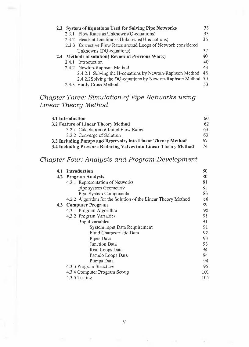
1.5 Method o f approach

(~ * ^Defining an appropriatepipe system

Defining Network elements Number o f pipes, junctions, loops, f lu id properties, p ipe characteristic (pipe diameter, length. Relative roughness), reservoir elevation, pum ps characters

Mass continuity equations are written

Conservative energy equations round loops are written

. aTransform the non-linear equations into linear equation using the technique o f Linear Theory M ethod

J3 -Solving the linear equations using Gauss elimination technique

From the calculated flo w rates, the head losses f o r each pipe is calculated.

Figure 1.1. Method o f approach for pipe networks simulation

1

1.6 Layout o f Thesis

This thesis is divided into six chapters. Following this introductory chapter, chapter 2

gives the platform for understanding the pipe network analysis, including the basic

principle of fluid mechanics, and also provides a better way of defining the pipe

network elements. The historical developments of the simulation of pipe networks are

reviewed and discussed, and the relevant literatures are given. Chapter 3 gives full

coverage of the linear theory method, which will be used to solve the pipe network

problems. Chapter 4 describes and discusses in details the development of the

program, which is based on the linear theory method. Also in this chapter, several

examples were presented and tested for the simulation. The results of the simulation

for several examples are presented and discussed in Chapter 5. Finally, conclusions

based on the present work are presented in Chapter 6.

8

CHAPTER 2

Pipe Network Analysis L iterature Review

2-1 Fundam ental Of Fluid M echanics

The aim of this section is to build on the understanding of the basic principles of

fluid mechanics so that one can apply these principles to the solution of pipe

network problems.

2 .1 .1 Fluid properties

Density: The mass per unit volume is referred to as the density of the fluid and is

denoted by the Greek letter (p). It is independent of gravitational force, but does

depend on temperature or pressure. For liquid, this dependence is very small and

can sometimes be ignored. The dimensions of density are mass per length cubed.

The English system of units (abbreviated ES) uses the slug for the unit of mass,

and feet for the unit of length.

Slue _ l b - sec2 — Or ------ —f t 3 f t

9

In the International system of units (abbreviated SI) which is an outgrowth of the

metric system, the mass is measured in the unit of the gram, gr. (or kg) and the

force is measured in Newton, N, and the length in meters,

kg ^ N -se c 23~ Am m

Specific weight: The specific weight is the weight of fluid per unit volume and is

denoted by the Greek letter (y)

The specific weight has dimension of force per unit volume .

Its unit in the ES is

]b_f l 3

and in the SI is

m2 - sec2

and the specific weight is related to the fluid density by the acceleration of gravity

T = gP

Viscosity: This fluid property has meaning when the fluid is in motion. It is a

measure of the fluid’s resistance to shear stresses. The viscosity is given the

symbol p and is defined as the ratio of the shearing stress t to the rate of change in

viscosity

In which the — is the derivative of the velocity with the respect to the distance dy

and called the velocity gradient

v = M- /p

2 .1 .2 Basic E quations

Solution to the most fluid flow problems generally involves the application of one

or more of the three basic equations: Continuity, Momentum, and Energy. These

three basic tools are developed from the law of conservation of mass, Newton’s

second law of motion, and the first law of thermodynamics.

2.1.2.1 Continuity equation

The simplest form of this equation is for one-dimensional incompressible steady

flow in a closed conduit.

AV = Q

in which A is the cross sectional area of the pipe, V is the average velocity of

the flow through the section, and Q is the volumetric flow rate.

In dealing with junctions of two or more pipes the continuity principle states that

the mass flow rate into the junction must equal the mass flow out of the junction.

Mathematically this principle is

= 0 (2-2)

This equation will play an important role in analysing networks of pipe [8,9].

11

The first law of thermodynamics states that the change of internal energy of a

system is equal to the sum of the energy added to the fluid and the work done by

the fluid. A general form of the energy equation for incompressible pipe flow

(assuming a uniform velocity profile) is

2.1.2.2 Energy equation

The unit of each term is energy per unit mass. The first two terms on both sides of

the equation are potential energy, the third term is the kinetic energy, WP is pump

energy added to the system, Wt is turbine energy removed from the system, and

Wf represents friction and other minor losses.

Equation (2.3) is restricted to steady flow and ignores nuclear, electrical, magnetic

and surface tension energy.

An alternate form of the energy equation is obtained by dividing equation (2.3) by

ft.lb N -m . . .gravity .The units are energy per unit weight of liquid: ---- or-------- , which

lb N

reduce to ft or m, respectively, after simplification, the form of the equation is

V- 2 - - Wn +W , + W f2 p I J (2.3)

H Z j +r

v+ z 2 + — H n + H . + H2g

(2.4)2 g r

In hydraulic engineering practice equation (2.4) is used more widely than

equation (2.3) and is known as the Bernoulli equation [8,9,10].

2 .1 .3 F riction Head L osses

Application of the energy equation requires an accurate estimate of the energy

losses caused by shear stress between the fluid and the boundary.

Equation (2.1) identifies that the shear stress is a function of viscosity and the

velocity gradient near the boundary .The velocity gradient is controlled by the

velocity, the boundary roughness, and thickness of the boundary layer [9].

The most significant problem with pipeline design is to obtain a reliable value of

the shear stress or pipe friction factor for fully developed flow or the loss

coefficients for local losses.

From an engineering point of view, it is not practical to work in terms of wall

shear stress since it requires detailed information on the velocity gradient. The

velocity gradient does not vary with distance in developed flow, but it is a

function of velocity and viscosity for fully developed flow.

It is easier to work in terms of the average shear stress or friction loss over a

length of pipe. The friction loss between two points in a pipe is equal to the

decrease in the total head. Dimensional analysis can be used to provide a

functional relationship between the friction loss, the important fluid properties and

flow parameters.

There are several equations that are often used to evaluate the friction head loss.

The most fundamentally sound method for computing such head losses is by

means of the Darcy-Weisbach equation.

13

a) Darcy-W eisbach equation

The Darcy -Weisbach equation is given by

A = ^ = / — (2.5)7 y 2gD

where D is the pipe diameter, L is the length of pipe, V is the average velocity

of flow, g is the acceleration of gravity and / is a dimensional friction factor

[9,11,12],

The friction factor / has been evaluated experimentally for numerous pipes.

Such tests have shown / to be a function of pipe diameter, roughness, and

Reynolds number Re.

Since roughness may vary with time due to build-up of solid deposits or organic

growths, / is also time dependent. Manufacturing tolerance also causes variation

in the pipe diameter and surface roughness. The point that is being made is that it

is not possible to know the friction factor of any pipe precisely.

A designer is required to use good engineering judgement in selecting a design

value for / so that proper allowance is made for these factors.

The functional relationship of f with roughness, diameter d, and Re has been

investigated quite thoroughly [9,12,13]. The pioneering work was done by

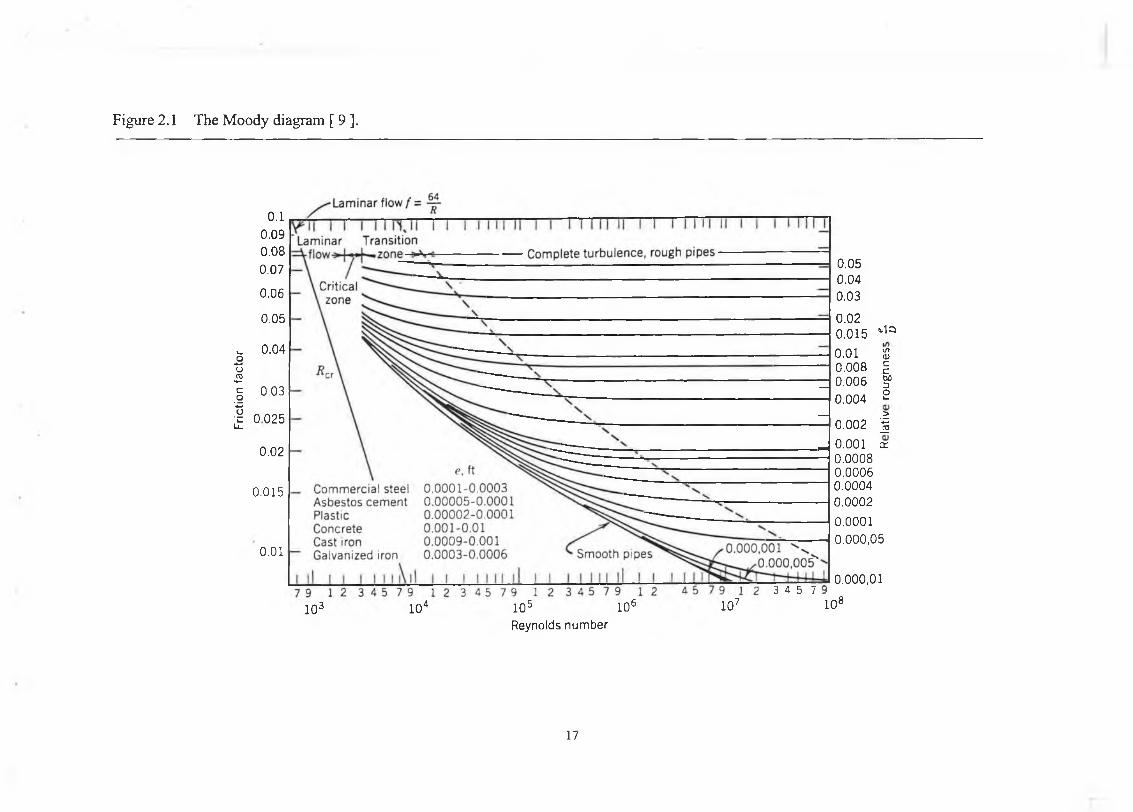
Nikuradse [12,13] and Colebrook [13,14]. Their work is the basis of the Moody

chart [9,13],

Nikuradse [13] measured head loss, or pressure drops, caused by bonding uniform

sand particles of various sizes, e, on the interior walls of different pipes. When his

test results are plotted on log-log graph paper with the Reynolds number,

14

R,VD

( 2 .6 )v

Plotted as abscissa and the friction factor / as the ordinate then data from

different values define the separate lines shown on Figure 2.1 [9,15],

Equation (2.5) is the basic equation from which the frictional pressure drop may

be calculated. It is valid for all types of fluid and for both laminar and turbulent

flow.

Friction factor for laminar flow

For laminar flow for which the well understood law of fluid shear, it is possible to

provide a simple straightforward theoretical derivation of the Darcy-Weisbach

equation, or more specifically derive the relationship

are summarised in Table 2.1 [12].

The pipes used by Nikuadse were artificially roughened with uniform roughness

and, therefore, can not be applied directly to commercial pipes containing

turbulent flows. Tests by others, notably Colbrook[l4 ],demonstrated that flows in

For /?e<2100 (2.7)

Friction factor for turbulent flow

Equations relating f to Rc and — for turbulent flow (i.e. flow with /ip >2100)

15

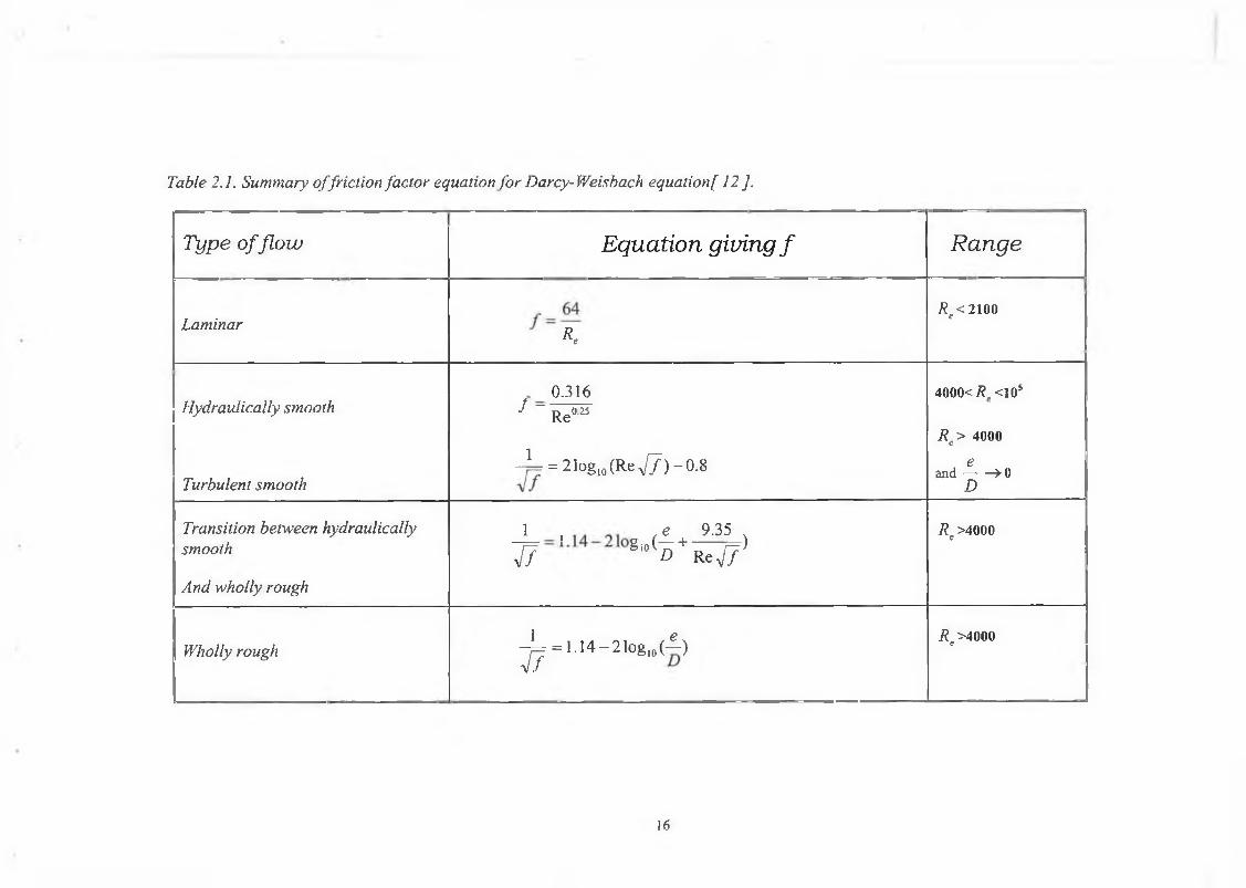
Table 2.1. Summary offriction factor equation for Darcy- Weis bach equation[ 12 J.

T ype o f f lo w Equation giving f Range

LaminarR,

Re< im

Hydraulically smooth

Turbulent smooth

0.316 J ~ Re0 “

- L = 2 l o g , 0 ( R e V 7 ) - 0 . 8

4000<Re<105

R > 4000ce

and----- > 0D

Transition between hydraulically smooth

And wholly rough

1 , , « 9-35 „4 7 8,0 V R e # ’

Re>4000

Wholly rough ^ - . . 1 4 - 2 t a * . < ± )Re>4000

16

Fric

tion

fact

or

Figure 2.1 The Moody diagram [ 9 ].

0.10.090.080.07

0.06

0.05

0.04

0.03

0025

0.02

0.015

0.01

0.050.040.03

0.020.015 *1c>0.01 is 0.008 _£ 0.006 g>0.004 2

>0.002 §0.001 tr 0.0008 0.0006 0.0004 0.0002 0.0001 0.000,05

0 .000,01

103 104 105 106 io7 lo8Reynolds number

3 4 5 7 9

17

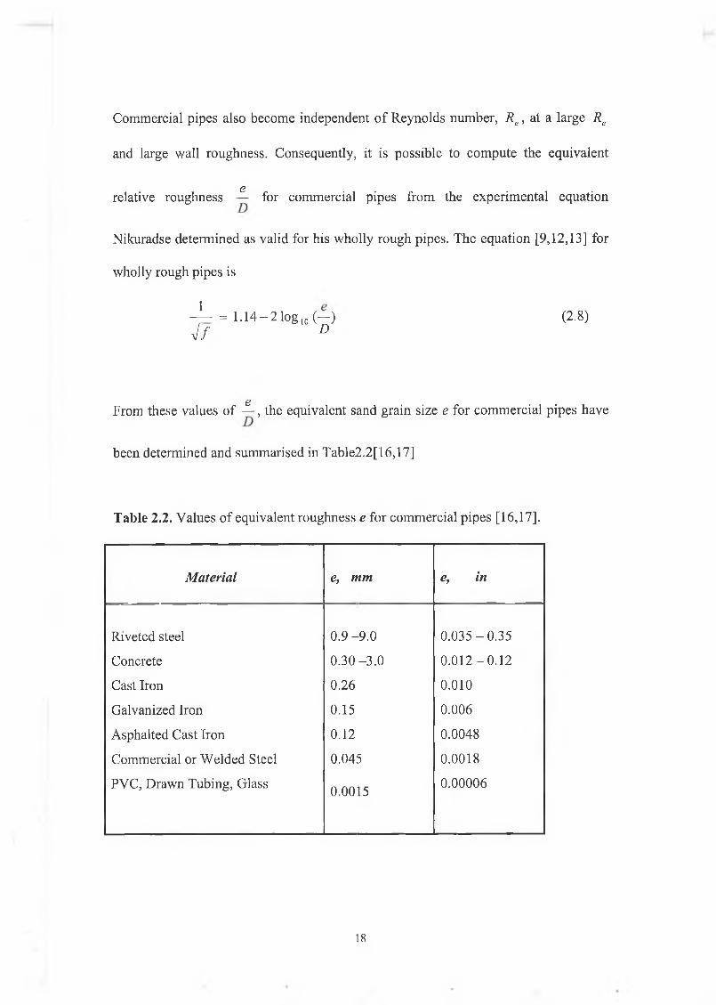
Commercial pipes also become independent of Reynolds number, Re, at a large Re

and large wall roughness. Consequently, it is possible to compute the equivalent

erelative roughness — for commercial pipes from the experimental equation

Nikuradse determined as valid for his wholly rough pipes. The equation [9,12,13] for

wholly rough pipes is

- L = 1.14-21og,0 ( - ) (2-8)4 f D

__ £From these values of — , the equivalent sand grain size e for commercial pipes have

been determined and summarised in Table2.2[16,17]

Table 2.2. Values of equivalent roughness e for commercial pipes [16,17].

Material e, mm e, in

Riveted steel 0.9-9.0 0.035-0.35

Concrete 0.30-3.0 0.012-0.12

Cast Iron 0.26 0.010

Galvanized Iron 0.15 0.006

Asphalted Cast Iron 0.12 0.0048

Commercial or Welded Steel 0.045 0.0018

PVC, Drawn Tubing, Glass 0.0015 0.00006

IB

For “hydraulically smooth” surface the equation is

- j j = 21ogm(ReA/ / ) -0 .8 (2.9)

The friction factor / appears on both sides of equation (2.9) and consequently it can

not be solved explicitly for / with Re known, but must be solved by trail and error

or some iterative scheme. An equation proposed by Blasius [12], which can be solved

explicitly for /'which apply to smooth pipes but only for flows with Re less than 10s ,

0316 ^J Re025 k '

Equation (2.9) applies to smooth pipe over the entire range of >4000,whereas

equation (2.10) is an approximation to equation (2.9) and is limited to the range

4000<Re<105.

For the transition zone between smooth and wholly rough flow, Colebrook and

White[12,14 ] give the following equation,

1 e 9.35= 1.14-2 log 10 (— + ------—) (2.11)

V7 D ReV7

Equation (2.11) gives nearly the same values for / as equation (2.9) for small values

£of — and values of / nearly equal to those of equation (2.8) for every large values

of Re. Consequently, equation (2.11) may be used to compute/ for all turbulent

flows [12].

19

Particularly for hand computations, it is convenient to summarise the equations in

Table 2.1 in a graph. This graph given as Figure 2.1 is known as the Moody diagram

[12,15], It is used to eliminate the trial and error solutions.

(b) Other empirical formulas

The Darcy-Weisbach equation is commonly used for determining head losses or

pressure drops in closed conduct flow because it is the most exact [13,17], This is

because the variation of / with pipe roughness and Reynolds number is properly

accounted for when the Moody chart is used. The two other equations in use are

1) Hazen-Williams equation

In ES units Q = l.3\SCHirAR°-63S 0M (2.12)

In IS units Q = 0M 9CHWAR™3 (2.13)

In which CHW is the Hazen-Williams roughness coefficient, S is the slope of the

h renergy line and equals to — , R is the hydraulic radius defined as the cross-sectionalL

area divided by the wetted perimeter, P and for pipes equals D/4.

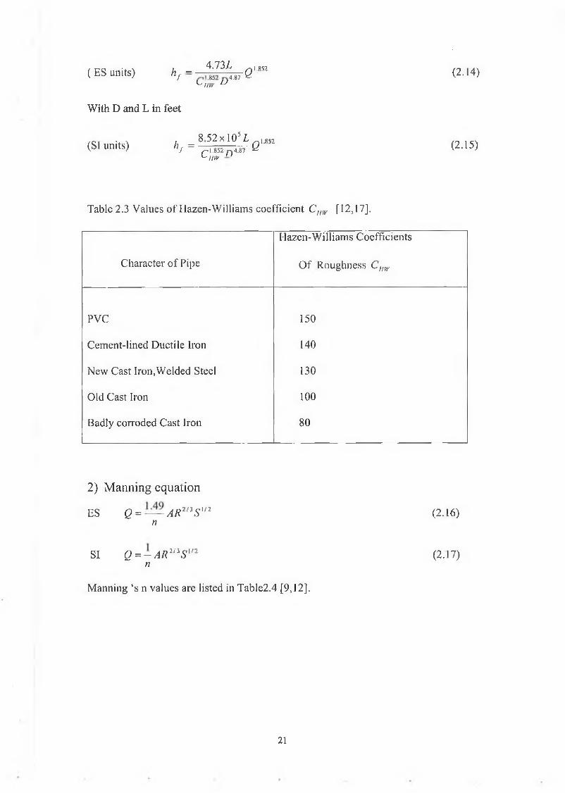
Suggested values of Hazen-Williams CHW are listed in table 2.3 [12,17]. Value of

CHW range from 140 for a new pipe in excellent condition to less than 100 for old

pipe in poor condition, typical values would be between 120 and 130 [17].

If the head loss is desired with Q known the Hazen-Williams equation for a pipe can

be written as

20

(E S “"its) h, - t ™ ; , , Q'm-mv u

(2.14)

With D and L in feet

(SI units) ^ = 8r ^ l V ‘" <2 '15)UW

Table 2.3 Values of Hazen-Williams coefficient Cuw [12,17],

Character of Pipe

Hazen-Williams Coefficients

Of Roughness C„w

PVC 150

Cement-lined Ductile Iron 140

New Cast Iron,Welded Steel 130

Old Cast Iron 100

Badly corroded Cast Iron 80

2) Manning equation

ES £? = — AR2nS 'n (2.16)n

SI Q = - A R 2nS '12 (2.17)n

Manning ‘s n values arc listed in Table2.4 [9,12].

21

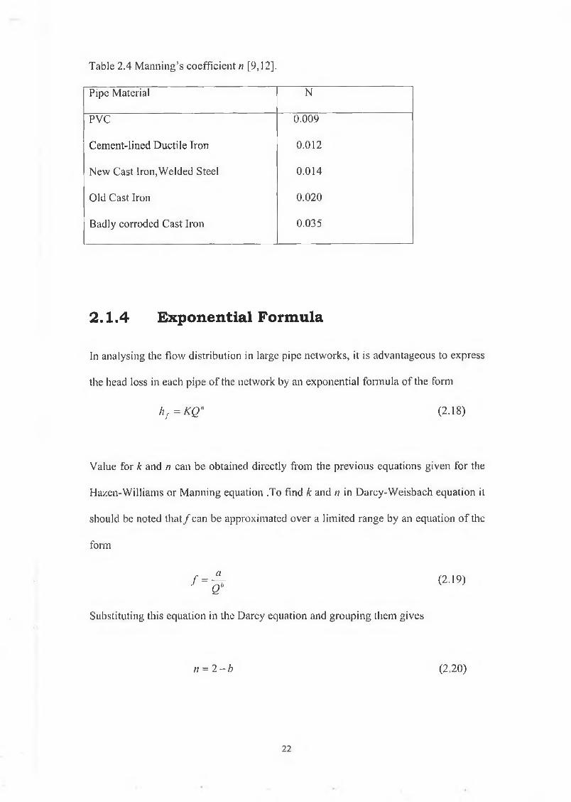
Table 2.4 Manning’s coefficient n [9,12].

Pipe Material N

PVC 0.009

Cement-lined Ductile Iron 0.012

New Cast Iron, Welded Steel 0.014

Old Cast Iron 0.020

Badly corroded Cast Iron 0.035

2 .1 .4 E xponentia l Form ula

In analysing the flow distribution in large pipe networks, it is advantageous to express

the head loss in each pipe of the network by an exponential formula of the form

hf =KQn (2.18)

Value for k and n can be obtained directly from the previous equations given for the

Hazen-Williams or Manning equation .To find k and n in Darcy-Weisbach equation it

should be noted that/can be approximated over a limited range by an equation of the

form

/ = J r (2.19)

Substituting this equation in the Darcy equation and grouping them gives

n = 2 - b (2.20)

22

and

k = (2.21)2 gDA2

Consequently determination o f n and k in the exponential formula requires finding

values o f a and b for the range o f flow rates to be encountered. If the range is too

large n and k may be considered variables [12,16,19],

2 .1 .5 Minor L osses

Minor losses is a term referring to losses that occurs at a pipe entrance, elbow, orifice,

valve, etc. These devices alter the flow pattern in the pipe creating additional

turbulence, which results in head loss in excess o f the normal frictional losses in the

pipe. These additional head losses are termed minor losses .If the pipelines are

relatively long these losses are truly minor and can be neglected. In short pipelines

they may represent the major losses in the system, or if the device causes a large loss,

such as a partly closed valves, its presence has dominant influence on the flow rate.

Judgement must be used in deciding how important the minor losses are and, therefor,

how much effort should be expended in evaluating the various loss coefficients

[8,9,11,17,20],

The head loss hf caused by a minor loss is proportional to the velocity head.

hL = K L^ (2.22)2gA

fLThe loss coefficient K L is analogous to — . I n fact, some prefer to express loss

coefficient as an equivalent pipe length [12,21,22]:

23

L = E l (2.23)D f

It simply represents the length o f pipe that produces the same head loss as the minor

loss. This is a convenient means o f including minor losses in the Hazen-Williams

and Manning equations.

For use with the Darcy equation, K L is used rather than equivalent length [21,22],

The total head loss terms in the energy equation can be written as

hf ^ ( y j ^ L-T + y j ^ ~ ) Q 2 = C Q 2 (2.24)1 ^ 2 gDA2 2gDA

The summation term represents the numerical sum o f all minor loss coefficients. If

the minor loss is different in diameter than the pipe, the proper area in equation (2.24)

must be used [12,13].

Typical value o f loss coefficient for various minor losses are summarised in Table2.5

Table 2.5 Minor Loss Coefficients [12,17]

Item

k l

typical value typical range

Bends

Short radius,r/d=l

90 0.24

45 0.10

Valves

Check valve 0.80 0.5 to 1.50

Full open gate0.15 0.1 to 0.3

Full open butterfly0.20 0.2 to 0.6

Full open globe 4.0 3 to 10

24

2-2 Incom pressib le stead y flow in p ipe netw orks

2.2.1 Introduction

Analysis and design o f pipe networks create relatively complex problems, particularly

if the network consists o f a large number o f pipes as frequently occurs in the water

distribution system o f a large metropolitan areas, or natural gas pipe networks.

Professional judgement is involved in deciding which pipe should be included in a

single analysis. Obviously it is not practical to include all pipes which deliver to all

sections o f the network, even though they are connected to the total delivery system.

Often only those main trunk lines that carry the fluid between separate sections o f the

area are included and if necessary analyses o f the networks within these sections may

be included.

In a water distribution or in any chemical complex pipelines network system, the

steady-state analysis is a small but vital component o f assessing the adequacy o f a

network.

Such an analysis is needed each time changing patterns o f consumption or delivery

are significant or add-on features, such as supplying new subdivision, addition of

booster pumps, or storage tanks change the system.

The steady-state problem is considered solved when the flow rate in each pipe is

determined under some specified patterns o f supply and consumption.

The supply may be from reservoirs, storage tanks and /or pumps or specified as

inflow or outflow at some point in the network.

From the known flow rates the pressure or head losses throughout the system can be

computed. Alternatively, the solution may be initially for the heads at each junction or

25

node o f the network and these can be used to compute the flow rates in each pipe in

the network.

2.2.2 Basic relations between network elements

The two basic principles, upon which all network analysis is developed, are (1) the

conservation o f mass or continuity principle, and (2) the work-energy principle,

including the Darcy-Weisbach or Hazen-Williams equation to define the relation

between the head loss and the discharge in a pipe[13,17]. The equations that are

developed from the continuity principle will be called junction continuity equations,

and those that are based on the work-energy principle will be called Energy Loop

Equations. The number o f these equations that constitutes a non-redundant system of

equations is related directly to fundamental relations between the number o f pipes,

number o f junctions and number o f independent loops that occur in a branched and

looped pipe networks[12,13,17]. In defining these relations NP will denote the

number o f pipes in the network. NJ w ill denote number o f junctions in the network,

and NL will denote the number o f loops around which independent equations can be

written. In defining junctions, a supply source will not be numbered as a junction. A

supply source is a point where the elevation o f the energy line, or hydraulic grade

line, is established. Figure 2.2 shows a sample o f the geometry o f simple pipe

network.

26

Source

/ Discharge

Pseudo loops

Figure 2.2. A small one real loop network and two pseudo loops connecting the supply sources

Pseudo loop I I source supply 1

Pseudo loop III

Reservoir

(5)

27

In general, pipe networks may include pipes in series, parallel pipes, and branching

pipes. In addition, elbows, valves, meters, and other devices which cause local

disturbances and minor losses may exist in pipes. All o f the above should be

combined or converted to an “equivalent pipe” in defining the network to be analyzed.

The concept o f equivalence is useful in simplifying networks. Method for defining an

equivalent pipe for each o f the above mentioned occurrences are as follows [13].

2.2.3.1 Series pipes

The method for reducing two or more pipes o f different sizes in series w ill be

explained by reference to the diagram below.

2.2.3 Reducing com plexity o f pipe networks

D i, Kj ,ni

Li

©2 j K2 , n2

Iu

The same flow must pass through each pipe in series. An equivalent pipe is a pipe

which will carry this flow rate and produce the same head loss as two or more pipes,

V. = 2 > /, (2-25)

Expressing the individual head losses by the exponential formula gives,

28

K tQM = k xQ" + k7Q*> +.... = 2 X 2 " ' (2.26)

For network analysis k and n are needed to define the equivalent pipe’s hydraulic

properties. If the Ilazen-William equation is used, all exponents n—1.85, and

consequently

or the coefficient k for the equivalent pipe equals the sum o f k o f the individual pipes

in series. If the Darcy-Weisbach equation is used, the exponents n in equation (2.26)

will not necessarily be equal, but generally these exponents are near enough equal to

that ne for the equivalent pipe can be taken as the average o f these exponents and

equation (2.27) may be used to compute K c [13,17],

2.2.3.2 parallel pipes

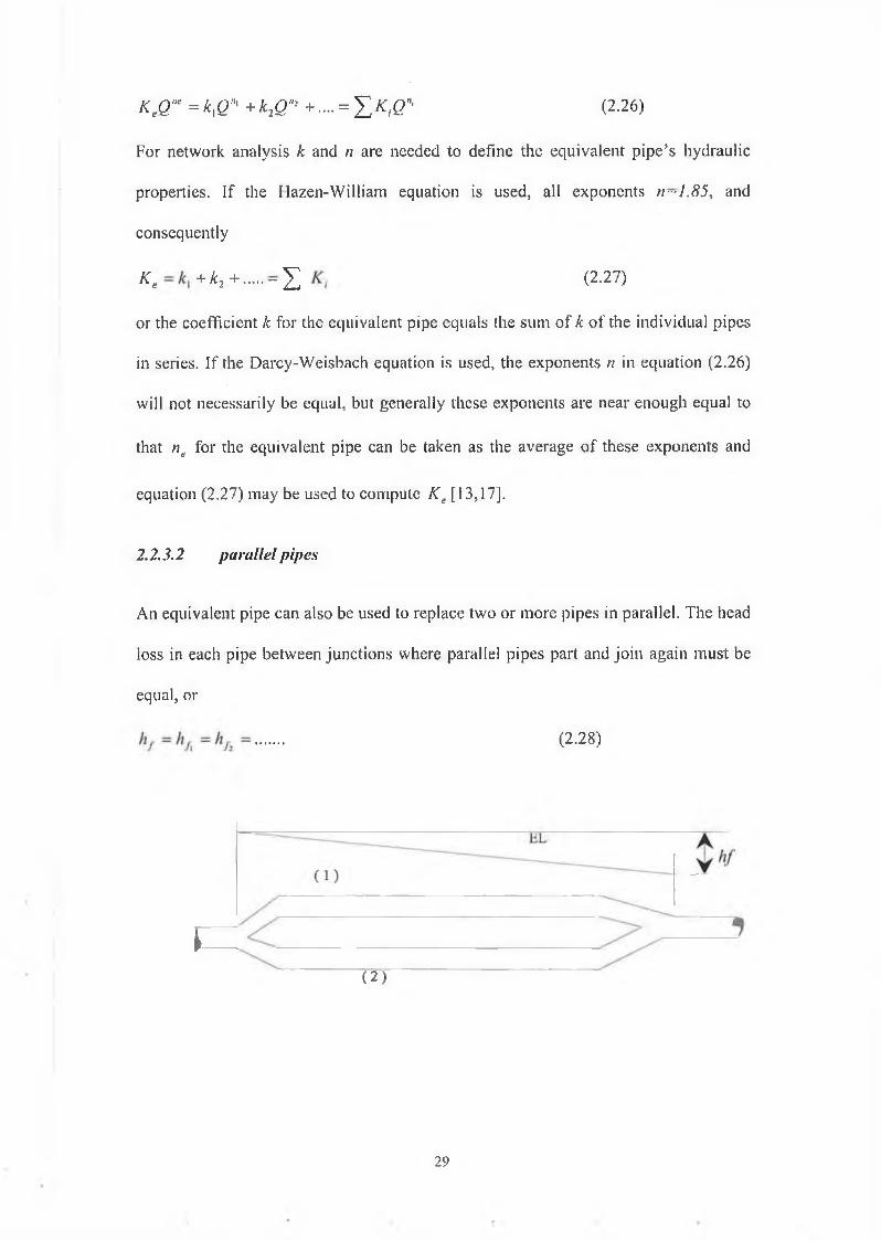
An equivalent pipe can also be used to replace two or more pipes in parallel. The head

loss in each pipe between junctions where parallel pipes part and join again must be

equal, or

K* +ki + “ X (2.27)

(2.28)

I

(2)

29

The total flow rate will equal the sum of the individual flow rates or

f i = e , + & + = I a (2-29)

Solving the exponential formula hf = KQ" for Q and substituting into equation (2.29)

gives

f i. \I 1

fu fu

K+

V /+ ....= Z

f L \(2.30)

If the exponents are equal as will be the case in using the Hazen-Williams equation

the head loss hf may be eliminated from equation( 2.30) giving

V*. /+

v ^ 2 J+ ..... = s (2.31)

When the Darcy-Weisbach equation is used for the analysis, it is common practice to

assume n is equal for all pipes and use equation (2.31) to compute the K e for the

equivalent pipe [12,13,17].

2.2.3.3 bran ch ing system

In a branching system a number o f pipes are connected to the main to form the

topology o f a tree. Assuming that the flow is from the main into the smaller laterals it

is possible to calculate the flow rate in any pipe as the sum o f the downstream

consumption’s or demands. If the laterals supply fluid to the main, as in a manifold,

the same might be done.

In either case, by proceeding from the outermost branches towards the main or “ root

of the tree” the flow rate can be calculated and from the flow rate in each pipe the

head loss can be determined using the Darcy-Weisbach or Hazen-Williams equation.

30

In analyzing a pipe network containing a branching system, only the main is included

with the total flow rate specified by summing those from the smaller pipes. Upon

completing the analysis the pressure head in the main will be known. By subtracting

individual head losses from this known head, the heads at any point throughout the

branching system can be determined [12].

2.2.3.4 minor losses

Valves and fittings in the piping system cause a minor loss, which is not insignificant

in comparison to the friction loss in a pipe.

The easiest way to calculate these losses is to use the equivalent length method to

estimate the effect o f a valve or fitting by treating it as if it were an additional length

of pipe. The equivalent pipe is formed by adding a length AL to the actual pipe length

such that the friction head loss in the added length o f pipe equals the minor

loss[l 2,21 ].

For use with the Darcy equation

/(2.32)

In the exponential formula , the K coefficient for the equivalent pipe is

+ X AL)

2gDA2(2.33)

Or might be given such as in Table [2.6] which lists some common devices and their

equivalent length values, which, are given as the length -to-diameter

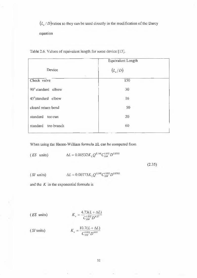
(Le /Z))ratios so they can be used directly in the modification o f the Darcy

equation

Table 2.6. Values o f equivalent length for some device [13].

Device

Equivalent Length

(¡■JO )

Check valve 150

90° standard elbow 30

45°standard elbow 16

closed return bend 50

standard tee-run 20

standard tee-branch 60

When using the Hazen-William formula AL can be computed from

( ES units) AL = O M 532K LQ omC l$ tD osm

(2.35)

(SJ units) AL = 0.00773KlQ°

and the K in the exponential formula is

(ES units)

( SI units)

32

_ 4 .7 3 (1 + A£)C ~ ,-,1.852 p . 4.87

W/jk u

_ 10.7(X + AL)c ^ .1 .852 n *1.87

W/H' U

2-3 S ystem o f equations u sed for so lv in g pipe netw orks

Three different systems o f equations can be developed for the solution o f network

analysis problems. These systems o f equations are named after the variables that are

regarded as the principal unknowns in that solution method. These systems o f

equations are called the Q-equations (where the discharges in the pipes o f the

network are the principal unknowns), the H-equations (where the HGL-elevation,

also simply called the heads H, at the nodes are the principle unknowns), and the AQ-

equations (when corrective discharges, AQ, are the principal unknowns). Each o f

these three systems o f equations will be studied separately.

2.3.1 Flow rates as unknowns (Q-equations)

The analysis o f flow throughout networks o f pipes is based on the two fundamental

laws o f fluid mechanics: continuity and conservation o f energy.

In addition, a relationship between flow rates, or velocity and head losses or pressure

drop is needed.

To satisfy continuity, the mass, weight, or volumetric flow rate into a junction must

equal the mass, weight, or volumetric flow rate out o f a junction.

For each junction a continuity relationship is written as:

E c s , ) » - S © ) « = c (2-36)

33

In which C is the external flow at the junction (commonly called consumption or

demand ). C is positive if flow is into the junction and negative if it is out from the

junction .

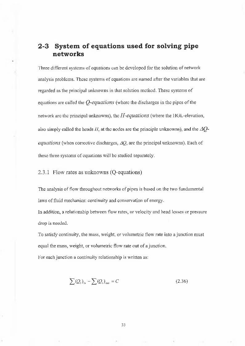
Consider four pipes meeting at a junction as shown in the sketch below.

If a pipe network contain M/junction, (also called nodes) and all external flow are known

then NJ-1 independent continuity equation in the form of equation (2.36) can be written.

The last, or the NJ'h continuity equation, is not independent; that is, it can be

obtained from some combination of the first N J -1 equations. Note in passing that

each of these continuity equations is linear, i.e., Q appear only to the first power

04

For applying the continuity equation to this example

03 + 0i + 02 + 04 ~ (2.37)

[12,13],

34

In addition to the continuity equations, which must be satisfied, the work-energy

principle provides additional equations, which must be satisfied.

These additional equations are obtained by summing head losses along both real and

pseudo loops to produce independent equations.

Mathematically, the energy principle gives

2 > j>= °/

(2.38)

NL

I

In which hf represents the head loss in a pipe contained in that loop and is a function

o f the discharge Q . And NL represents the number o f non-overlapping loops (also

referred to the real loops) in the network, and the summation on small / is over the

pipes in the loops I, II,... , NL by use o f the exponential formula hf = K Q ".

However, the head loss in pipe ( i) is best represented by a relationship

f j K ,Q ;L = 0 (2.39)t

A pipe network consisting o f Adjunction and NL real loops and NP pipes will satisfy

the equation

NP = (NJ - l ) + N L (2.40)

(if all o f the external flows are not known ,then all NJ junction equations are

independent and available for u se ).

The ( NJ-1 ) continuity equations are linear and the NL ( head losses ) equations are

non-linear.

35

Systematic methods, which will utilize computer, are needed for solving this system

of simultaneous equations [12,13,18]

2.3.2 Heads at junctions as unknowns (H-equations)

If the elevation o f the energy line or hydraulic grade line throughout a network is

initially regarded as the primary set o f unknown variables, then one develops and

solves a system of H-equations. One H-equation is written at each junction. Since

looped pipe networks have fewer junctions than pipes, there w ill be fewer

H-equation than Q-equations. Every equation in this smaller set is non-linear,

however, whereas the junction continuity equations are linear in the system of

Q-equations .

To obtain the system o f equations, which contain the heads at the junctions o f the

network as unknowns, the NJ-1 independent continuity equations are written as

before. Thereafter the relationship between the flow rate and head loss is substituted

into the continuity equations. In writing these equations, one begins by solving the

exponential equation for the discharge in the form

i i

i M% [ h . - h A

1 s?

K J K, J

Here the frictional head loss has been replaced by the difference in HGL(hydraulic

grade line) values between the upstream and downstream nodes. In addition, in this

equation a double subscript notation; has been introduced; the first subscript defines

the upstream node o f the pipe, and the second defines the downstream node. Thus Qy

and K y denote the discharge and loss coefficient for the pipe from node i to node j .

36

Substituting equation (2.41) into the junction continuity equations, equation (2.36),

yields

IEH , - H , L - [ I \ -

L = c (2.42)

Upon writing an equation o f the form of equation (2.42) at NJ-/junctions, a system of

NJ-1 nonlinear equations is produced [12,13,23],

2.3.3 Corrective flow rates around loops of network considered unknowns (AQ-equations)

Since the number o f junctions minus 1 (i.e.NJ-1) will be less in number than the

number o f pipes in a network by the number o f loops NL in the network, the last set o f

H-equations will generally be less in number than the system o f Q-equations. This

reduction in number o f equations is not necessarily an advantage since all o f the

equations are non-linear, whereas in the system o f Q-equations only the NL energy

equations were non-linear. A system that generally consists o f even fewer equations

can be written for solving a pipe network, however. These equations consider a

corrective flow rate in each loop or Q ’s as the unknowns.

These corrective discharges will be determined from the energy equations that are

written for NL loops in the network, and thus NL o f these corrective discharge

equations must be developed. To obtain these equations, we replace the discharge in

each pipe o f the network by an initial discharge, denoted by Qoi, plus the sum of all

o f the initially unknown corrective discharges that circulate through pipe i, or

a = a , + 2 > & (2 .4 3 )

37

In equation (2.43) the summation includes all of the corrective discharges passing

through pipe i , the initial discharges Qoi must satisfy all of the junctions continuity

equations. It is not difficult to establish the initial discharge in each pipe so that the

junction’s continuity equations are satisfied. However, these initial discharges usually

will not satisfy the energy equations that are written around the loops of the network

[12].

To establish NL energy loop equations around the NL loops of the network, in which

each discharge plus the sum of corrective loop discharges, Qk is used as the

discharge. The junction continuity equations are satisfied by the initial discharge

Qoi and are not a part of the system of equations. The corrective discharges can be

chosen as positive if they circulate around a loop in either the clockwise or counter

clockwise direction. It is necessary to be consistent within any one loop, but the sign

convention may change from loop to loop, if desired. A corrective discharge adds to

the flow Qoi in pipe i if it is in the same direction as the pipe flow, and it subtracts

from the initial discharge if it is in the opposite direction.

To summarise how the AQ -equations are obtained, replace the Q ’s in the energy loop

equations, equation.( 2.38) and equation (2.39) by

& = a , ± Z A&

Using the notation t for the NL energy equations around the basic loops can be

written as,

i ___X K, (Qd + Ag[)"' = 0 (Head loss around loop I)

u ,X + A£?2)"' = 0 (head loss around loop II)

38

X (Got + AQe)n' = 0 (Head loss around loop t ) (2.44)i

In which each summation includes only those pipes in the loop designated by the

Roman numeral I, II... V., and AQt always includes A£?,and also any other

AQ's flowing through the pipe for which the terms applies [12].

39

2 .4 M ethods o f so lu tion(Review o f previous work)

2.4.1 Introduction

Pipe networks may include serial pipes, parallel pipes and branching pipes, in addition

to elbows, valves, meters and other devices that cause local disturbances and minor

losses. There are several calculation techniques available to analyse flow rates and

pressures or head losses throughout the pipe system.

One of the first and oldest method and the most widely used method of analysis is the

Hardy Cross technique [7]. This method makes corrections to initial assumed values

by using a first order expansion of the energy equation in terms of a correction factor

for the flow rate in each loop. The process is, of course, repetitive and is dependent on

the accuracy of the initial guess, which must be reasonably good if an answer is to be

obtained rapidly. This method is well suited for solution by hand

Usually the Hardy Cross method is used to determine heads and flows in pipe

network.

Essentially the usual Hardy Cross method consists of “guessing “ the flow rate @

In each pipe and then systematically revising these flow rates based on the fact that

algebraic sum of all head losses in each loop should be zero. The computed sum of

the head losses around a loop based on the assumed flow rates will ordinarily not be

zero. The deviation from zero may be used to calculate a correction. When the

correction applied to the assumed flow rates, a better approximation of the true flow is

obtained. The correction process is carried out over the network until it is believed

40

that the flow rates are close enough to the real values for the purposes at hand

[7,19,23,27].

Numerous computer programs based on the Hardy-Cross procedure have been

developed [19,24,25,26]

In certain cases, it has been found that the Hardy Cross method converges very slowly

or not at all. This has led McCormick and Bellamy [28] and McCormick [29] to

suggest special measures to improve convergence.

A second method which is being applied successfully to hydraulic network analysis

utilizes the Newton-Raphson method to formulate a set o f simultaneous linear

equations which can be solved for flow corrections for each loop in the network. This

method is described by Martin and Peters [6,30] for studies o f hydraulic networks.

The method has been extended by Shamir and Howard [31] to include various

hydraulic components in the network such as pumps and valves in place o f pipes

between two joints. Martin and Peters[6] and Shamir and Howard [31] developed a

method o f solving for unknown flow resistance with known heads. Epp and Fowler

[32] have described a technique using Newton’s method to solve a system of

simultaneous equations along with information on how to reduce the number of

equations required and the input data needed.

Because this method adjusts the flow rate in all the loops simultaneously,

convergence using the Newton-Raphson approach is much quicker than that obtained

using the Hardy Cross analysis[32,33]. This is especially important when analyzing

networks involving large numbers o f pipes. However, both methods o f analysis

require an initial guess for flow distributions, and very bad estimates o f these values

41

can lead to slow convergence or, in some cases, a situation where the successive trails

do not converge and the solution can not be found.

Other analytical methods have been proposed for hydraulic network problems but

have not gained wide acceptance. For example, Warga [34] applied Duffm’s [35]

work on non-linear networks to hydraulics networks

Direct electrical analogies are also used for hydraulic network analysis, most popular

is the fluid network analyser developed by Mclllroy [36], This and other available

direct analogue devices are described in a paper by McPerson [37],

Other analytical methods and most widely used to solve hydraulic network problems

has been developed in recent years.

The Linear Theory Method described by Wood and Charles [5] is the method used to

solve for the pipe flow and can also be regarded as an application o f the Newton-

Raphson technique in the sub-domain o f loops. The number o f independent continuity

and energy equations equals the number o f pipe sections for all network

configurations. The resulting equation set is non-linear and is expressed in terms o f

the unknown flow rates in the pipe sections. The solution is obtained by applying the

Newton-Raphson procedure to linearize non-linear terms and solving the resulting

system of linear simultaneous equations. But it requires the solution o f a large system

of equation (number o f loops and number o f nodes) although reducing the risk o f the

failures. Wood and Rayes [38], Ormsbee and Wood [39,40], Boulos and Wood [41],

Issac and Mills [42] and Nelson [43] developed this method to improve the

convergence o f the solution. The method has been extended by Jepson and Travallaee

42

[18] , Jepson and Davis[44] to include various hydraulic components in the network

such as pumps and pressure reducing valves.

Many computer programs based on this method are described by Wood [17], Jepson

[12], and Larock, Jepson and Watters [13] have described methods for improving the

efficiency of solution of some of these methods when applied to a large networks.

As a first step in developing a computer program using C language, various methods

of analysis have therefore been reviewed. Some of these are presented herein.

2.4.2 Newton-Raphson method

The Newton-Raphson method uses an iterative process to approach one root of a

function[l,3].

In using the Newton-Raphson method the equation containing the unknown (which

will be called x when describing the method in general), is expressed as a function

which equals zero when the correct solution is substituted into the equation or

f(x) = 0. The Newton-Raphson method computes progressively better estimate of

the unknown x by the formula,

----------------------------------- (2-45)/ ( * w ) y V ” )

43

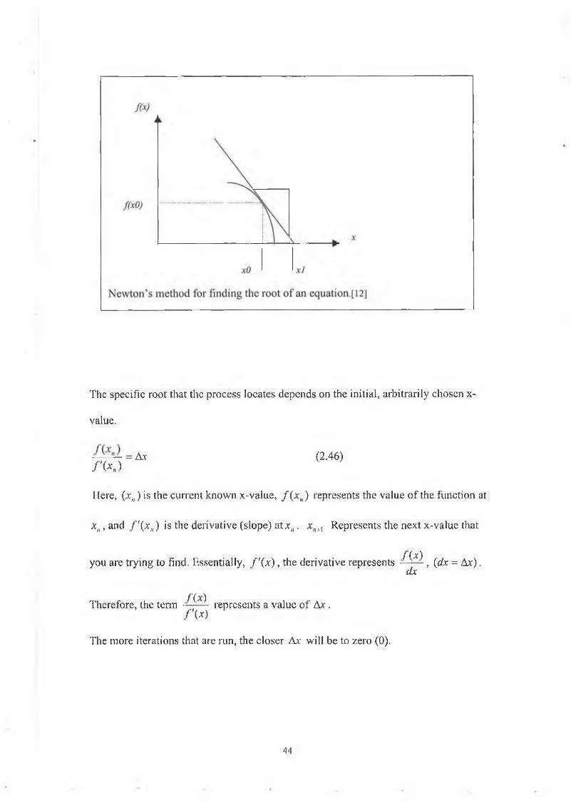
The specific root that the process locates depends on the initial, arbitrarily chosen x-

value.

= Ax (2.46)f ' M

Here, (xn) is the current known x-value, f ( x n) represents the value of the function at

xn, and f ' ( x n) is the derivative (slope) atxn. xn+1 Represents the next x-value that

f i x )you are trying to find. Essentially, f ' ( x ) , the derivative represents , (dx = Ax).

dx

f(x)Therefore, the terra —— ~ represents a value of Ax. f \ x )

The more iterations that arc run, the closer A y will be to zero (0).

44

The Newton-Raphson method may be used to solve any of the three sets of equations

describing flow in pipe networks which are discussed in next section.

The equations considering:

1-The How rates in each pipe unknown

2-The head at each junction unknown

3-The corrective flow rate around cach loop unknown.

The Newton-Raphson method requires an initial guess to the solution.

The iterative Newton-Raphson formula for a system of equations is ,

The unknown vector x and F f replace the single variables and function F and

the inverse of the Jacobian D~l , replace in the Newton-Raphson formula for

dx

solving a single equation.

If solving the equation with the heads as the unknown (i.e.theH - equations) the

vector x becomes the vector I I .

If solving the equations containing the corrective loop flow

rates (i.e.iheAQ - equations) x becomes AQ .

The individual elements for vector// and vector AQ are

45

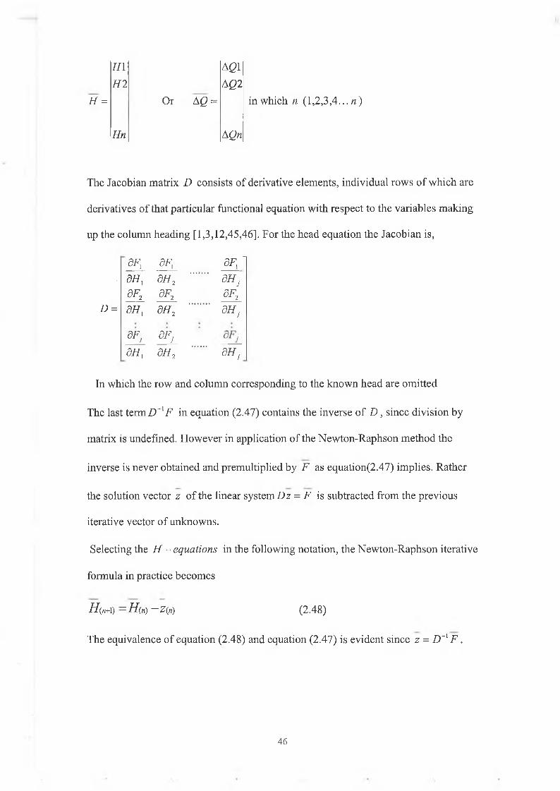
H =

HI AQlHI AQ2

Or A Q =

Hn AQn

in which n (1,2,3,4... n)

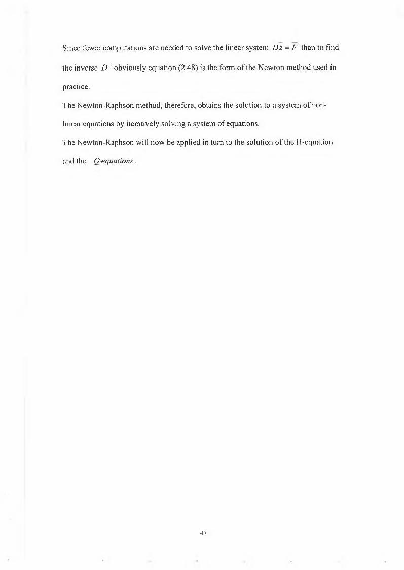
The Jacobian matrix D consists of derivative elements, individual rows of which are

derivatives of that particular functional equation with respect to the variables making

up the column heading [1,3,12,45,46]. For the head equation the Jacobian is,

dF '

D =

dF, dF,dH, dH2dF2 dF2dH{ 5H2

dF] dFj8H{ dH2

dHjdF2

d H J

dHj

In which the row and column corresponding to the known head are omitted

The last term D~lF in equation (2.47) contains the inverse of D , since division by

matrix is undefined. However in application of the Newton-Raphson method the

inverse is never obtained and premultiplied by F as equation(2.47) implies. Rather

the solution vector z of the linear system D z = F is subtracted from the previous

iterative vector of unknowns.

Selecting the H -equations in the following notation, the Newton-Raphson iterative

formula in practice becomes

H(n+1) =H(n) ~Z{n) (2.48)

The equivalence of equation (2.48) and equation (2.47) is evident since z = D~[ F ,

46

Since fewer computations are needed to solve the linear system Dz = F than to find

the inverse D~x obviously equation (2.48) is the form of the Newton method used in

practice.

The Newton-Raphson method, therefore, obtains the solution to a system of non­

linear equations by iteratively solving a system of equations.

The Newton-Raphson will now be applied in turn to the solution of the H-equation

and the O-equations .

41

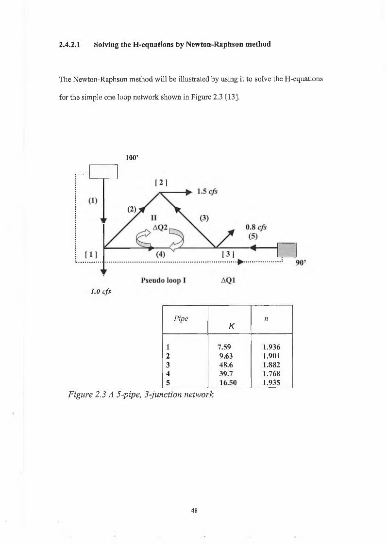
2.4.2.1 Solving the H-equations by Newton-Raphson method

The Newton-Raphson method will be illustrated by using it to solve the H-equations

for the simple one loop network shown in Figure 2.3 [13].

100 ’

J.Ocfs

PipeK

n

1 7.59 1.9362 9.63 1.9013 48.6 1.8824 39.7 1.7685 16.50 1.935

Figure 2.3 A 5-pipe, 3-junction network

48

Simplify the problem the IIazen-Williams equation will be used so that k and n in the

exponential formula are constant. Since there are 3 junctions and the heads are

unknown and to be determined, one must construct three 11-equations.

They areo 0 1 »i h , - h 2 )»2

- 1 . 0 = 0I ) K> J l J

1 I\ ~ f I , 7 1 \»2 + UJ 1 St! K> %

3 —1.50 = 0I *2 J I *3 JI I I

«4 ÎU 1

to 1

+

r 90 - I l 3 ) He- 0 . 8 - 0

* 4 J I * 3 J V * 5 y

Using Dz = F and H(n+i) —H(n) ~Z(n) to implement the Newton method.

The Jacobian matrix

dFx dF\ ÔF{dH\ ôh2 ÔH,ÔF2 ôF2 ÔF2a//, ôh2 dH,ôf2 0F, ôf2Ô//| ôh2 ÔH3

Using Dz = F and H(„+\) — H \n) —Z(„) to implement the Newton method

With an initial estimate of the nodal heads as

'H i '93'{H}° = h 2 = 85

H 3 . 88_

The solution to

49

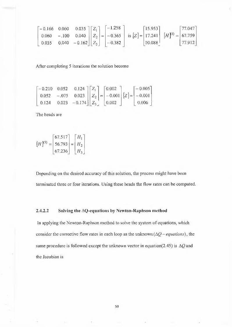
'-0 .166 0.060 0.035 ' ’z i '-1.258 ' '15.953' '77.047'

0.060 ! o o 0.040 Z2 = - 0.365 is [z ] = 17.241 lHP = 67.759

0.035 0.040 — 0.162 „Z3. -0.382 10.088 77.912

After completing 5 iterations the solution become

' - 0.210 0.052 0.124 ' ~zi "0.002 '-0 .0 0 5 '0.052 -.075 0.023 Z2 = -0.001 [ Z h -0.0010.124 0.023 — 0.174 A . 0.002 0.006 _

The heads are

'67.517"[h }5) = 56.793 = Ht

67.236

Depending on the desired accuracy of this solution, the process might have been

terminated three or four iterations. Using these heads the flow rates can be computed.

2.4.2.2 Solving the AQ-equations by Newton-Raphson method

In applying the Newton-Raphson method to solve the system of equations, which

consider the corrective flow rates in each loop as the unknown (AQ - equations) , the

same procedure is followed except the unknown vector in equation(2.45) is Agand

the Jacobian is

50

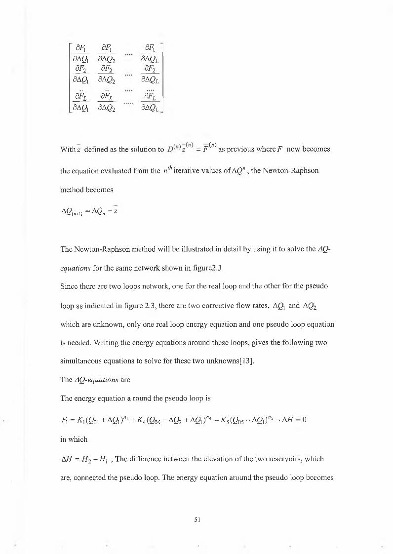
BFl dFl dFyda a dAQ2 dA QldF2 qf2 sf2

dA f l 8AQ2 3A Ql

8Fl 8Fl

•co

dA a dAQ2 9A Ql

Withz defined as the solution to = F ^ as previous whereF now becomes

the equation evaluated from the nth iterative values of A Q" , the Newton-Raphson

method becomes

A0(n+1) = A0„ - z

The Newton-Raphson method will be illustrated in detail by using it to solve the AQ-

equations for the same network shown in figurc2.3.

Since there are two loops network, one for the real loop and the other for the pseudo

loop as indicated in figure 2.3, there are two corrective flow rates, AQl and AQ2

which are unknown, only one real loop energy equation and one pseudo loop equation

is needed. Writing the energy equations around these loops, gives the following two

simultaneous equations to solve for these two unknowns[13].

The AQ-equations are

The energy equation a round the pseudo loop is

Fx = ^(001 + A a r +^4(004 -AQ 2 + Aft)"4 -^5(005 - A 0)"5 - AH - 0

in which

AH = H2- H{ , The difference between the elevation of the two reservoirs, which

are, connected the pseudo loop. The energy equation around the pseudo loop becomes

51

F, = * ,< & ,+ AS,)“' + K i (Qu -A Q 2 + AQlf< - K s(e 05 - AQ)"> -10 = 0

The energy equation around the real loop is

F2 = K2(Q02 + AQ2r + ^3(003 - AC?2)"3 - ^4(004 - A02 + A j a r = 0

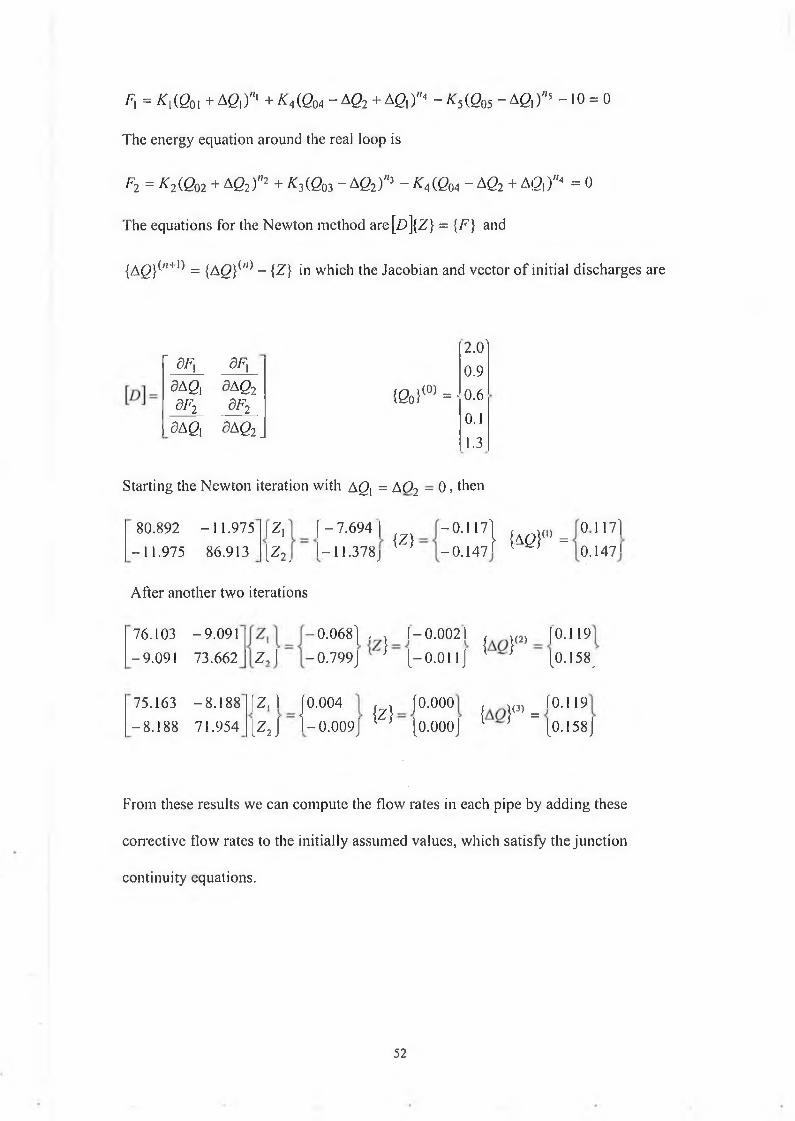
The equations for the Newton method are[£>]{Z} = {F} and

{A<2} "+l) = {Ag}(,,) - {Z} in which the Jacobian and vector of initial discharges are

2.0'' dFx dF{ 0.9dA Q{ dF2

dAQ2dF2 {0O>(O) = • 0.6

dA Q, oaq2_ 0.11.3

Starting the Newton iteration with AQX = A0 2 - 0, then

{Z}1 1.J /oj

After another two iterations

80.892 -11.975-11.975 86.913

I*.1*2.

(-7.694 j 1-11.378

- ° - U 7l { « } < » .0117]-0.147 1 0.147

76.103 -9.091 -9.091 73.662

0.068)Z j

, j l - 0 . 0 0 2 1 { }(2) [0.119- 0.799J [-0.01 lj 1 * [0.158 J

75.163 -8.188 -8.188 71.954

[Z J j 0-004 {z} fO.OOO { j(3)= f0.119[Z2 J 1-0.009J 1 J [O.OOOj 1 j [0.158 J

From these results we can compute the flow rates in each pipe by adding these

corrective flow rates to the initially assumed values, which satisfy the junction

continuity equations.

52

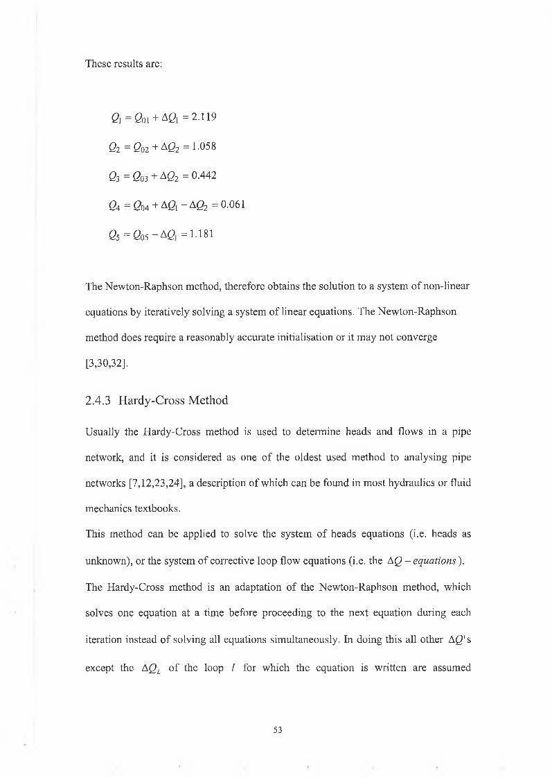
These results are:

0 = 0 ) 1 + Aft =2.119

02 = 002 + A02 = 1 -0^8

03 = 003 + A02 = 0.442

0 4 — 0 0 4 + A 0 1 _ A 0 2 — 0.061

0 5 = 0 0 5 - A 0 ! =1.181

The Newton-Raphson method, therefore obtains the solution to a system of non-linear

equations by iteratively solving a system of linear equations. The Newton-Raphson

method does require a reasonably accurate initialisation or it may not converge

[3,30,32],

2.4.3 Hardy-Cross Method

Usually the Hardy-Cross method is used to determine heads and flows in a pipe

network, and it is considered as one of the oldest used method to analysing pipe

networks [7,12,23,24], a description of which can be found in most hydraulics or fluid

mechanics textbooks.

This method can be applied to solve the system of heads equations (i.e. heads as

unknown), or the system of corrective loop flow equations (i.e. the A Q - equations).

The Hardy-Cross method is an adaptation of the Newton-Raphson method, which

solves one equation at a time before proceeding to the next equation during each

iteration instead of solving all equations simultaneously. In doing this all other AQ's

except the AQL of the loop I for which the equation is written are assumed

53

temporarily known. Based on this assumption, the Newton-Raphson method can be

used to solve the single equation F, = 0 or for AQL, or

(2.49)

It is common in the Hardy-Cross method to apply one iterative correction to each

equation before proceeding to the next equation.

After applying one iterative correction to all equations the process is repeated until

convergence is achieved. Furthermore, it is common to adjust the initially assumed

flow rate in all pipes in the loops o f that equation immediately upon computing each

Consequently each equation F, — 0 is evaluated with a llA ^ 's equal to zero, and

furthermore the previous AQ}"° consequently equation (2.49) reduces to,

The superscript denoting iteration numbers in equation(2.49) are deleted in

equation(2.50) because only one AQ appears. The equation Ft = 0 for / loop is the

head loss equation around the loop or

A£.

(2.50)

d m )

54

F, = T . k ,.q ; (2.51)

The derivative of F, is,

Substituting equation (2.51) and equation (2.52) into equation (2.50) gives the

following equation by which the Hardy-Cross method computes a corrective a flow

rate AQ, for each loop of the network.

AQ 'E M (2.53)

If the Hazen-Williams equation is used to define K and n in the exponential formula,

then equation (2.53) simplifies to

1 .8 5 2 3 (C //» 0 ,.e os52

55

The Hardy-Cross method is outlined in the following procedure:

Step 1. Assume an initial flow rate for each pipe such that all junction continuity

equations are satisfied.

Step 2. Compute the sum of head loss around a loop of the network. Care must be

taken to maintain proper signs. This step computes the numerator of equation (2.53)

Step 3. Compute the denominator of equation (2.53) by accumulating the absolute

values of niKiQ"i~[ around the same loop.

Step 4. Compute AQ by dividing the result from step 2 by the result from step 3

Step 5. Repeat steps 2 through 4 for each loop in the network.

Step 6. Repeat the iterative procedure (steps2 through 5) until all AQ ’s computed are

sufficiently small to be neglected. [8,12]

The calculation method is illustrated by the following example problem:

A pipe network can be divided into two flow loops shown in figure 2.4.

Initial guesses of the flow rates in each pipe are selected, obeying continuity at the

junction of each section.

Head losses are computed in the clockwise direction. Table 2.7. Tabulates values for

the iterative procedure.

For the first iteration the difference for loop (I) is

1197NQj = — = -0 A 9 csf

1.852(13207)

56

- 5 8 4 9A Q„ = --------- — -------- = 1.98csf

“ 1 .852(1593)

For loop (II),

These differences are unacceptable. Adding the AQ ’s to the initial flow rates provides

estimates for the second iteration.

For the second iteration,

- 1 4 3A Q, = --------------------- = 0 .06csj

I 1 .852(1317)

- 1 7 4 0AQn = ----------= 0 .7 6csf

1.852(1242)

A0, Is acceptable; AQ„ is not acceptable. A third trial is needed for loop (II), so is

added to the second iteration flow rates. Finally, for the third iteration convergence is

achieved:

AQ = ------ ~ 1QQ6 = 0 .05c s fII 1 .852(1087)

57

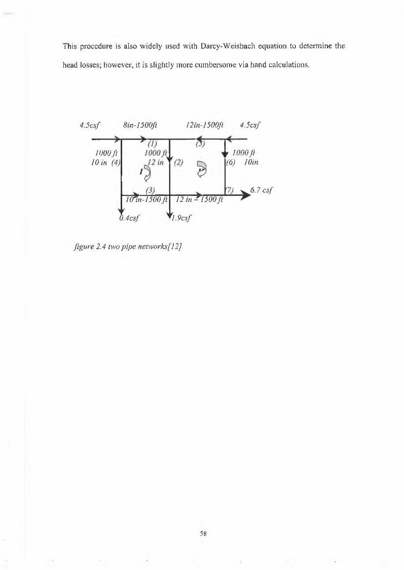
This procedure is also widely used with Darcy-Weisbach equation to determine the

head losses; however, it is slightly more cumbersome via hand calculations.

4.5csf 8in-l500ft

1000ft 10 in (4)

12in-l 500ft 4.5csf

¡000 ft (6) Win

7) ^ 6.7csfI (Tin-1500ft

f.

0.4csJ

12 in -1500 ft

1.9csf

figure 2.4 two pipe networks[12]

58

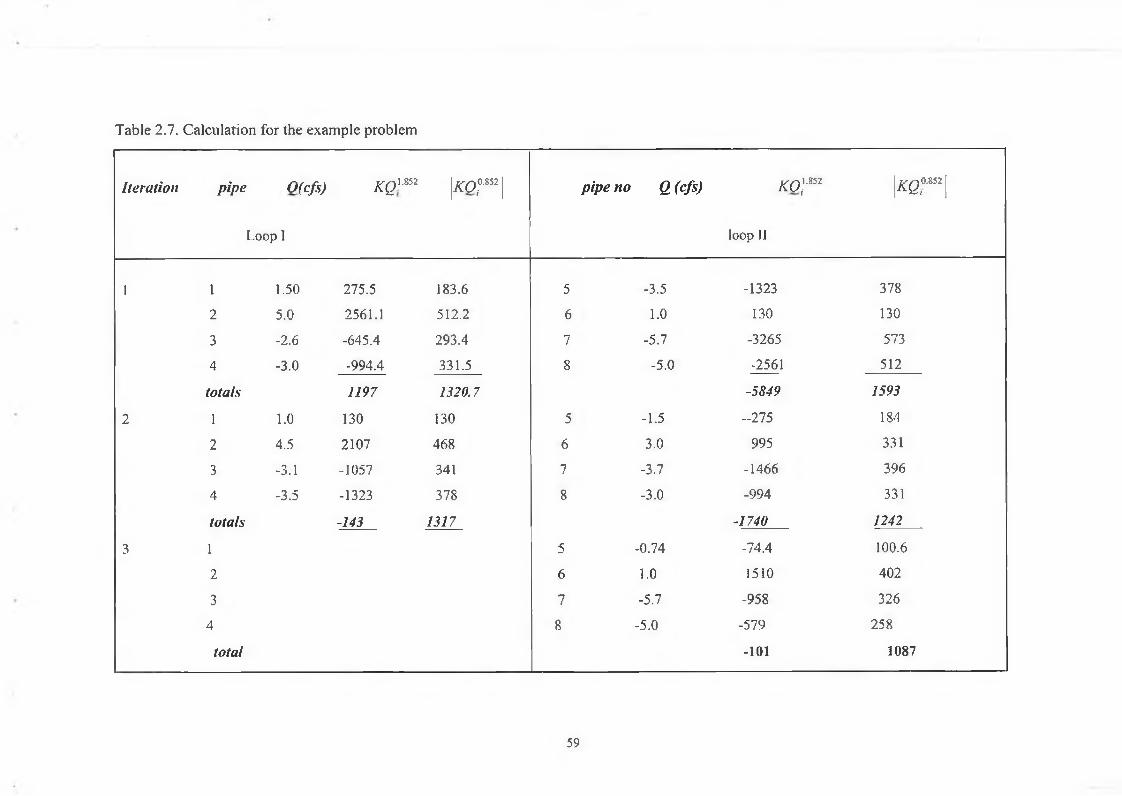
Table 2.7. Calculation for the example problem

Iteration pipe O(efs)

Loop I

K Q I . S S 2 \k o ?™\ p ipe no Q (cfs) K O ^ 52

loop II

|*e,aS52|

1 1 1.50 275.5 183.6 5 -3.5 -1323 378

2 5.0 2561.1 512.2 6 1.0 130 130

3 -2.6 -645.4 293.4 7 -5.7 -3265 573

4 -3.0 -994.4 331.5 8 -5.0 -2561 512

totals 1197 1320.7 -5849 1593

2 1 1.0 130 130 5 -1.5 -2 7 5 184

2 4.5 2107 468 6 3.0 995 331

3 -3.1 -1057 341 7 -3.7 -1466 396

4 -3.5 -1323 378 8 -3.0 -994 331

totals -143 1317 -1740 1242

3 1 5 -0.74 -74.4 100.6

2 6 1.0 1510 402

3 7 -5.7 -958 326

4 8 -5.0 -579 258

total -101 1087

59

CHAPTER 3

Simulation of pipe networks using linear Theory method

3.1 in trod u ction

The solution to a problem of steady-flow distribution in a pipe network is obtained when

the flow satisfies both the continuity equation at each junction and the energy equation in

each pipe.

In this project the linear theory method will be described and used in solving the system

of equation, which considers the flow rates known.

This system of equation is easy to use if all external flows to the system are known.

The linear theory method will be described first for solving the system of Q-equation,

thereafter it will be extended to networks containing pumps and reservoirs. For such

networks, not all-external flows are known, and must be obtained as part of the solution.

In a network of NP pipes and Adjunction and NL loops, it has been shown that the

following identity holds [12,13]:

NP = (Ad + NL) - 1 ........................... (3.1)

This is true for networks with all closed loops, for open tree -type networks, or

combination of both type set is possible to write Ad -1 linear continuity equations

60

(The additional equation is redundant) for all but one of the junctions in the network

stating that the discharge into the junction equals the discharge out of the junction

q, - a . . . . . . . . . . . . . . . . . . . . . ( 3 - 2 )In which Q = the volumetric discharge. In addition there are energy equations (one for

each loop) of the form:

2 > / = 0............................... (3.3)

In which hf represents the head loss in a pipe contained in that loop and is a function of

the discharge, Q .

From equation ( 3.2 ) and equation. (3.3) n simultaneous equations are obtained in terms

of the discharge in each pipe. Theoretically, the equations could be solved for the

discharge. However, the head loss in pipe i is best represented by a relationship

(3 .4)

In which Ki a pipeline constant which is normally a function of line length, diameter and

type of pipe material, and n an empirical head loss exponent usually ranging between 1.8

and 2.0 for turbulent flow [5,12,17,18], This relationship makes each of the NL loop

equations non-linear and no method is known for the direct solution of this set of

simultaneous equations.

61

3.2 Feature o f linear th eory m eth od

Linear theory transforms the NL non-linear loop equations into linear equations by

approximating the head loss in each pipe by,

*/, =kerb=if;a (3.5)In which Qio = the approximate discharge in line i. When Qi0 approaches the actual

discharge, Qn equation (3.5) becomes an exact expression of the head loss. Using values

for approximate discharge to compute the modified pipeline constant K[ the loop

equation can be expressed as linear equations which when combined with the continuity

equations yield n linear simultaneous network equations which can be readily solved for

the discharge in each line [5,12,18,38],

However, this is an approximate solution as approximate values for the discharge are

used to linearise the head loss terms. The computed values for discharge can then be used

to compute a new values for the modified pipeline constant, K \ which are used to obtain

a new set of n simultaneous equations which can be solved for improved values for line

discharge. This process can be continued until the discharges obtained from two

successive sets of calculations do not differ significantly.

It has been found that there are several features of this method, which make it attractive

for hydraulic network calculations.

62

3.2.1 Calculation o f Initial flow rates

The method requires an estimate of flow rate in each line .The converge of the solution is

greatly affected by the accuracy of the initial estimates and very poor estimates can lead

to a situation where the solution will not converge. For the linear theory method it is not

necessary to estimate initial flow rates, instead, reasonably accurate initial flow rates can

be easily calculated. This is done by assuming that the modified pipeline constant is

independent of flow rate [5,12,13,38] and, as a first approximation, is given by

K't = K tQ ? (3.6)

That is the coefficient K' is defined for each pipe as the product of K j multiplied by

Q"~[ , an estimate of the flow rate in that pipe. Combining these artificial linear equations

with the junction continuity equations provide a system of n linear equations which can

be solved by linear algebra.

The solution will not necessarily be correct because the Qh ’s will probably not have

been estimated equal to the Qt ’s produced by the solution. By repeating the process ,after

improving the estimate oi'Qi ,eventually the Qi0 ’s will equal the Qj ’s after few

iteration.

3.2.2 Converge of solution

In applying the linear theory method it is not necessary to supply an initial guess ,as

perhaps implied .Instead for the first iteration each K \ is set equal to K i, which is

63

equivalent to setting all of the flow rates Qi0 equal to unity .Wood [5] in developing the

linear theory method observed that successive trials always gave a result which

converged to the correct solution but the result of successive trial tended to oscillate

about the final result .He also noted that the average of two successive trials gave a result

very close to the final value of the flow rate. Therefore, the average values of the two

prior sets of calculations for flow rate were used to compute the best value of the

discharge for the trial and the modified pipe line constant, K\ , which was used for the

next trial [5,12,13].

This is expressed as

a . = a -,+2 a -1 (3 .7 )

In which Q._{ =the flow rate obtained from the previous trial for the line I and

Qi 2 = The flow rate obtained for the trial previous to that

The first step is to obtain K and n for the exponential formula for a range of flow rate to

be realistic.

In implementing the method in the computer program the first values used for K and n

may be obtained from the Hazen-William equation (2.14 and 2.15)[12,13],

To illustrate the Linear Theory Method, consider the small 5-pipe network shown in

figure 3.1. Since no supply sources are shown for this network, only NJ-1 junction

continuity equations are available.

64

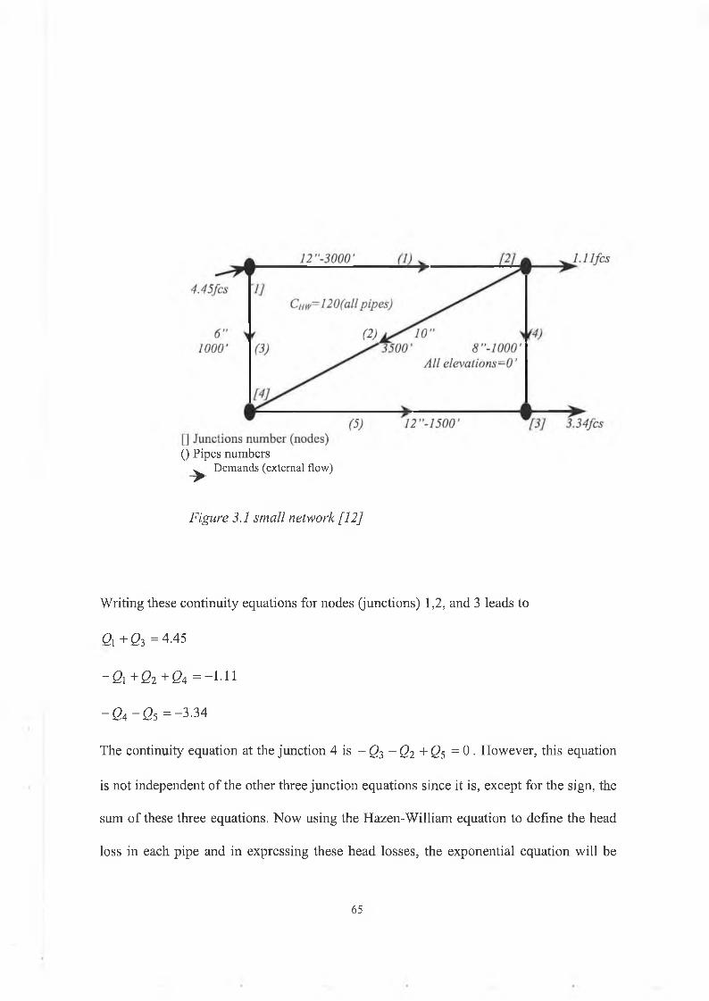
() Pipes numbers ^ Demands (external flow)

Figure 3.1 small network [12]

Writing these continuity equations for nodes (junctions) 1,2, and 3 leads to

<2,+ 0 3 =4.45

“ 01 + 0 2 + 0 4 = “ I ' l l

- 0 4 - 0 5 = - 3 . 3 4

The continuity equation at the junction 4 is - Q3 - Q2 + 0 5 = 0 . However, this equation

is not independent of the other three junction equations since it is, except for the sign, the

sum of these three equations. Now using the Hazen-William equation to define the head

loss in each pipe and in expressing these head losses, the exponential equation will be

65

used. From equation (2.14) the K coefficients for the exponential formula are the

following

K,=2.018, K=5.722,K=19.674,K=4.847,K=1.009

The energy equations around the two real loops may be written as

K {Ql*52+ K 2Ql2*52- K 3Q \S52=0

k 4q \*52- k 5q 15*52- k 2q \ S52=0

These two energy equations are obtained by starting at junctions 1 and 2, respectively,

and moving around the respective loops I and II in a clockwise direction. If the assumed

direction of flow opposes this traverse, a minus sign precedes the head loss term for that

pipe. These simultaneous equations, such as those above, are called Q-equations because

it is the Q ’s, that are the set of primary variables.

To solve the system of these simultaneous equations Gauss elimination technique is used,

which is one of most widely used methods to solve simultaneous equations, and it will be

discussed as part of the simulation (see appendix A).

After the Q ’s are found, the head losses in each pipe can be determined. From a known

head or pressure at one junction it is then a routine computation to determine the heads

and pressures at each junction throughout the network.

In some problems the external flows may not be known as was assumed in the above

example. Rather, the supply of fluids may be from reservoirs and/or pumps. The amount

of flow from these individual sources will not only depend on the demands, but also will

depend upon the head losses throughout the system. Method for incorporating pumps and

reservoirs into a network analysis using Linear Theory Method will be illustrated in the

next section.

66

3.3 Including Pum ps and Reservoirs in to L inear Theory M ethod

All applications o f the linear theory method described previously were for networks in

which the external flows were assumed known. In practice this may not be the case.

Rather the amount o f flow being supplied from different reservoirs or pumps will depend

upon the heads and flows throughout the network. Consequently the utility o f the linear

theory method can be enhanced by extending it to handle supply source from reservoirs

or pumps, and allow booster pumps to exist within pipelines.

Each pump (not a booster pump) and each reservoir from which flow enters or leaves the

system introduces an additional unknown that must be solved for in solving the network.

Since pumps and reservoirs must be connected to the network by a pipe through which

they supply the flow, it is natural to let the flow rates in these connective pipes be the

additional unknown. However, elevation o f reservoirs, and the elevations o f reservoirs

from which pumps obtain the fluid plus the pump characteristics (i.e. h versus Qp) are

known for pumps. Therefore equations are needed which relate these known to the

connective pipe flow rates.

If one reservoir and one pump supply the flow to the network, as shown in the sketch

below, such that flows in two connective pipes becomes additional unknowns, one

additional equation is necessary beyond the N J available continuity equations and the

NL available energy equations.

A convenient means for obtaining this additional equation is by defining a so called

67

Pseudo loop, which connects the two reservoirs by “no flow”, pipe as illustrated below.

Note those two pumps and / or reservoirs must be present or the network reduces to one

for which all external flows are known.

Consequently such pseudo loops can be always be defined, because at least two

reservoirs and / or pumps must exist in the network if all external flow rates are not

known. The additional needed equation (or equations if more than two pumps and /or

reservoirs are present), comes from the energy equation around this pseudo loop.

Around pseudo loops the sum o f the head loss is not equal to zero but must account for

the difference in reservoirs elevations or head produced by the pump or pumps [12,18].

No flow pipe

Figure 3.2 small pipe network including pumps

68

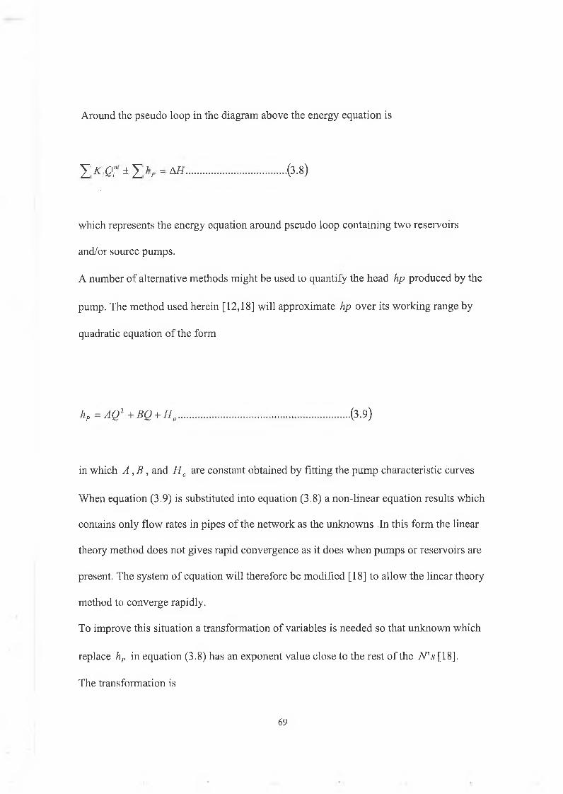
A r o u n d th e p s e u d o lo o p in th e d ia g r a m a b o v e th e e n e r g y e q u a t io n is

' Z K iQ:“ ± Y hr = AH (3.8)

which represents the energy equation around pseudo loop containing two reservoirs

and/or source pumps.

A number o f alternative methods might be used to quantify the head hp produced by the

pump. The method used herein [12,18] will approximate hp over its working range by

quadratic equation o f the form

in which A , B , and H o are constant obtained by fitting the pump characteristic curves

When equation (3.9) is substituted into equation (3.8) a non-linear equation results which

contains only flow rates in pipes o f the network as the unknowns .In this form the linear

theory method does not gives rapid convergence as it does when pumps or reservoirs are

present. The system o f equation will therefore be modified [18] to allow the linear theory

method to converge rapidly.

To improve this situation a transformation o f variables is needed so that unknown which

replace hP in equation (3.8) has an exponent value close to the rest o f the N's [18].

The transformation is

hP - AQ 1 + BQ + H t .(3.9)

69

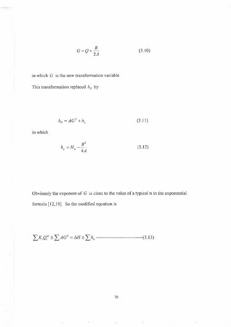
G = Q + ~ (3.10)2 A

in which G is the new transformation variable

This transformation replaced hF by

hp = AG 2 + h 0 (3.11)

in which

B 2K = h . - Va (3.12)

Obviously the exponent o f G is close to the value o f a typical n in the exponential

formula [12,18]. So the modified equation is

.(3.13)

70

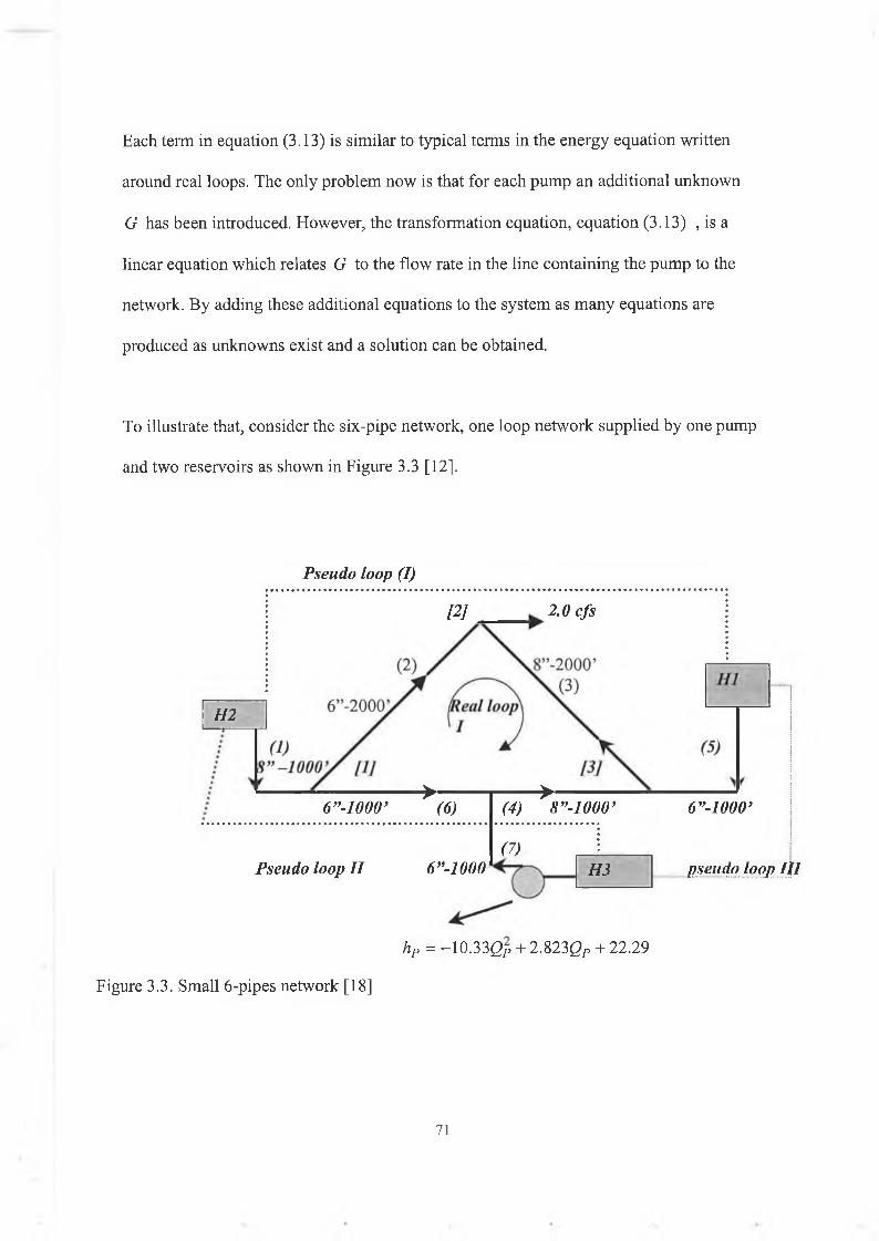
Each term in equation (3.13) is similar to typical terms in the energy equation written

around real loops. The only problem now is that for each pump an additional unknown

G has been introduced. However, the transformation equation, equation (3.13) , is a

linear equation which relates G to the flow rate in the line containing the pump to the

network. By adding these additional equations to the system as many equations are

produced as unknowns exist and a solution can be obtained.

To illustrate that, consider the six-pipe network, one loop network supplied by one pump

and two reservoirs as shown in Figure 3.3 [12].

Pseudo loop (I)

[2] 2.0 cfs

112

> > ------------6”-1000’ (6) (4) 8”-1000’ 6 ”-1000’

(7)Pseudo loop II 6”- l 000 H3 pseudo loop III

hP = -10.330p + 2.8230p + 22.29

Figure 3.3. Small 6-pipes network [18]

71

Since there are six pipes in this network there will be six unknown flow rates, plus one

additional unknown, i.e. the G o f equation for the pump which supplies the flow from the

reservoir 3.

Four junction continuity equations are available. They are the following:

-0 1 + 0 2 + 0 6 = 0 (3.14a)( 1)

-0 2 - 03 =-2-0 (3.14b)(2)

03 - 04 - 05 = 0 (3.14c)(3)

0 4 - 0 6 - 0 7 = 0 (3.14d)(4)

The number o f energy loop equations is NL=NP-NJ=7-3=4 (one for the real loop and the

other three for the pseudo loops connection reservoirs with no pipe flow. But there are 7

unknowns, so one o f the pseudo loop will be ignored since only two pseudo loops

required.

The number o f pseudo loop equation generally available equals the sum o f the reservoirs

and source pumps minus one or

Ls=Nr+NPS-l (3.15)

A possibility is one pseudo loop connecting the reservoirs supplying pipes 1 and 5

through pipes 1,6,4,and 5; and the other connects the pump reservoir and the reservoir

supplying pipe 1 through pipes 1,6, and 7.

The three energy equations are

K 2Q ¥ - K 3Q? - K 4QHa - K 6Qn6* = 0 (real loop) (3.16 a)

72

K\Q"X + K GQ'l6 - K 1Q"'> + V, = AH = H 2 - H3 =100-95 (pseudo loop 4 II) (3.16 b)

KiQ['1 + K bQ lb + K 4Q - K SQs'5 = A ll = H 2 - H l =100-105 (pseudo loop I) ( 3 .16c)

The head produced by the pump can be defined by a second-order polynomial passing

through three points o f the pump curve as described earlier, so

hPl = A Q 2 + BQ + H 0

hP | = AG2 +h0

Equation (3.16b) become

KxQP + K6Q^b - K 7Q ? + AG , = A H - h 0 = 100 - 9 5 - h0

the additional unknown is G , by applying the equation (3 .10 ), the transformation

equation can be written as follow

- Q i +G[ = — (Transformation equation ) (3.17)2 A

there are now eight independent equations that contain the seven unknowns discharges

0 / , Q2, .....C?7, P*us additional unknown G

In applying the linear theory method, the three nonlinear energy equations are linearized

as described previously, and the resulting system solved.

In summary then, if pumps or reservoirs exist in a pipe network, a solution by the linear

theory method accomplished as follow:

1- NJ linear junction continuity equations are written

73

2- NL non-linear energy equations are written around the real loops o f the system

3- Additional pseudo loops are defined which connect supply reservoirs or reservoirs

from which pumps obtain their supply by no flow pipes.

Energy equations are written around these pseudo loops. These energy equations

contain a new unknown Gi for each pump in the network. The number o f these

pseudo loops must equal the difference between the number o f unknown flow rate,

i.e. NP and (NJ+NL ).

Jg4- as many additional linear equations o f the form G = Q + — are written as pumps

2 A

exist

5- The non-linear energy equations are linearized by defining coefficients K" o f the Q ’s

equations which are obtained by K" = K Q Mn~[ and coefficient K"G for the G unknown

are obtained by K ”G = AG

6-the resulting system is solved iteratively, adjusting the coefficients as described earlier

to reflect the average o f the flow from the past two solutions until convergence occurs

[12,18,44],

3 .4 Including Pressure R educing V alves in to Linear Theory M ethod

A pressure reducing valves (denoted PRV) is designed to maintain a constant pressure

downstream from it regardless o f how large the upstream pressure is.

The exceptions to this occurrence are: (1) if the upstream pressure becomes less than the

valve setting, and (2) if the downstream pressure exceeded the pressure setting o f the

74

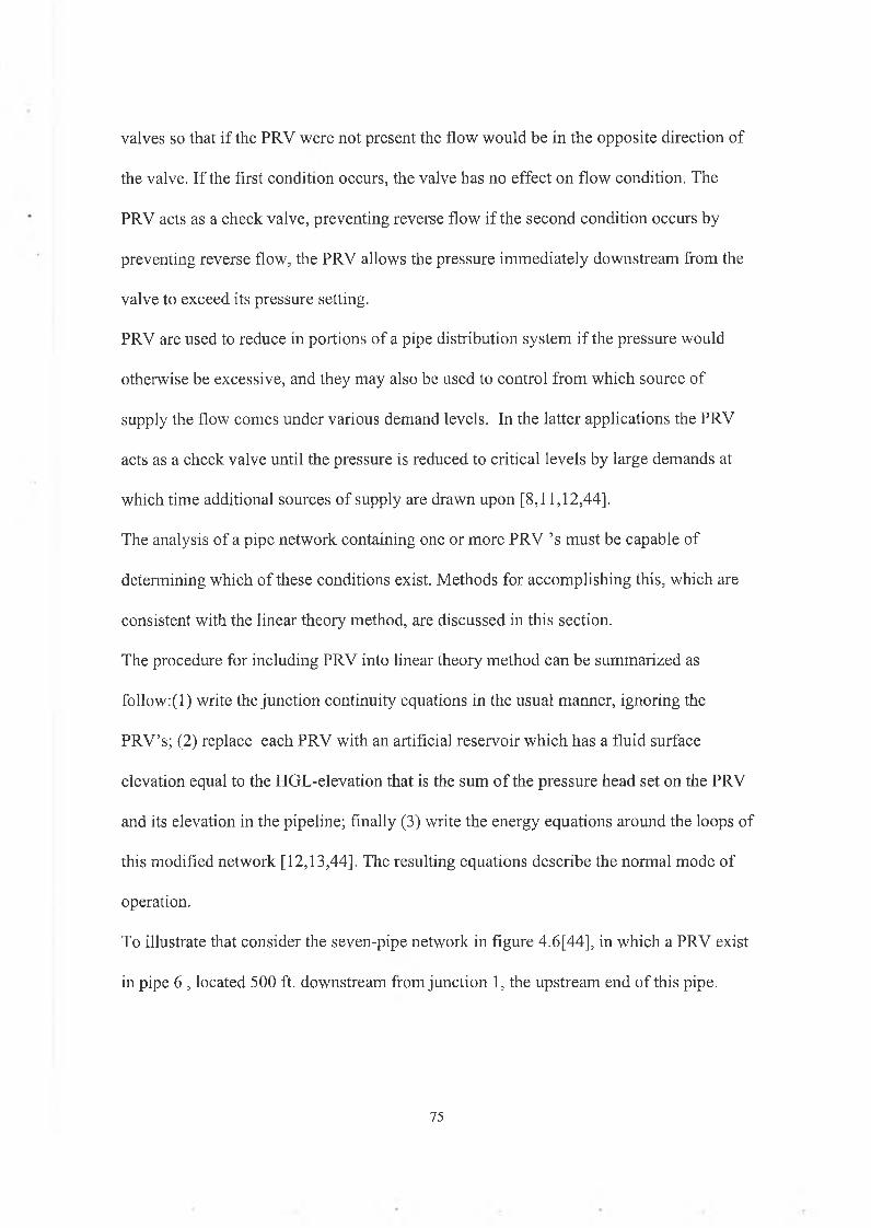
valves so that if the PRV were not present the flow would be in the opposite direction of

the valve. If the first condition occurs, the valve has no effect on flow condition. The

PRY acts as a check valve, preventing reverse flow if the second condition occurs by

preventing reverse flow, the PRV allows the pressure immediately downstream from the

valve to exceed its pressure setting.

PRV are used to reduce in portions o f a pipe distribution system if the pressure would

otherwise be excessive, and they may also be used to control from which source of

supply the flow comes under various demand levels. In the latter applications the PRV

acts as a check valve until the pressure is reduced to critical levels by large demands at

which time additional sources o f supply are drawn upon [8,11,12,44],

The analysis o f a pipe network containing one or more PRV ’s must be capable of

determining which o f these conditions exist. Methods for accomplishing this, which are

consistent with the linear theory method, are discussed in this section.

The procedure for including PRV into linear theory method can be summarized as

follow:(l) write the junction continuity equations in the usual manner, ignoring the

PRV’s; (2) replace each PRV with an artificial reservoir which has a fluid surface

elevation equal to the HGL-elevation that is the sum o f the pressure head set on the PRV

and its elevation in the pipeline; finally (3) write the energy equations around the loops of

this modified network [12,13,44], The resulting equations describe the normal mode of

operation.

To illustrate that consider the seven-pipe network in figure 4.6[44], in which a PRV exist

in pipe 6 , located 500 ft. downstream from junction 1, the upstream end o f this pipe.

75

Since a PRV is a directional device , one must always identify the upstream and

downstream ends o f the pipe containing it.

The system of Q-equation for this network consists o f four junction continuity equations

and three energy equations obtained from loops. The junction continuity equations are

identical to those that would be written if the PRV were not present and they are:

76

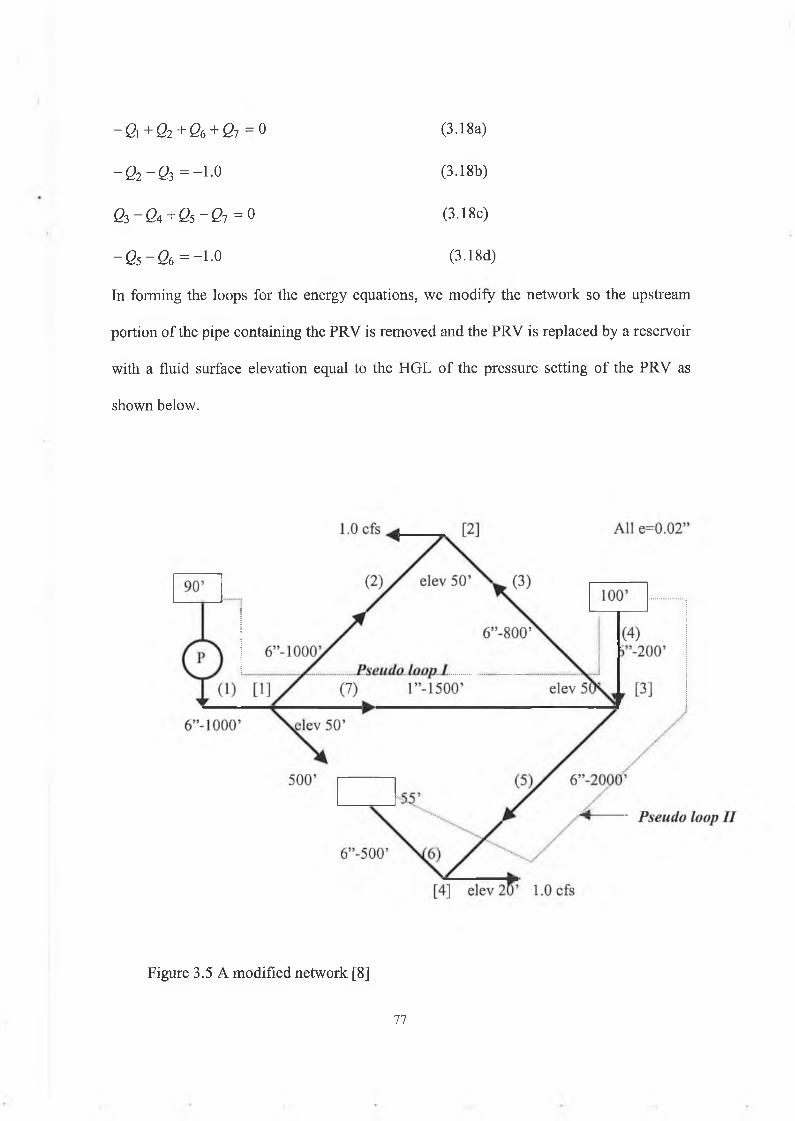
- 0 2 - 0 3 = -1 -0 (3.18b)

03 - 04 + 05 - 07 = 0 (3.18c)

- 0 5 - 0 6 =-1-0 (3.18d)

In forming the loops for the energy equations, we modify the network so the upstream

portion o f the pipe containing the PRV is removed and the PRV is replaced by a reservoir

with a fluid surface elevation equal to the HGL o f the pressure setting o f the PRV as

shown below.

~Q \ + 02 + 06 + 07 ~ 0 (3.18a)

Figure 3.5 A modified network [8]

77

Of the three loops that exist in this modified network, only one is a real loop, which

traverses pipes 2, 3, and 7. Two pseudo loops also exist. One pseudo loop connects the

two original supply sources. This loop can start at the reservoir and the end at the source

pump so it includes pipes 4, 7, and 1. The second loop must extend from the artificial

reservoir created by the PRY to one of the other supply sources. The shortest path for this

second pseudo loop will traverse pipes 4,5,and 6 . Note that with pipe 6 disconnected

from junction 1 , only one real loop is available whereas two independent real loops

existed before. The real loop, which is lost through the disconnection, is compensated for

by the additional pseudo loop from the artificial reservoir created by the PRV.

A modified loss coefficient K' will be used to denote this change in the exponential

formula. The new coefficient K' equals the K for the pipe containing the PRV,

multiplied by the ratio of the pipe length from the PRV to the pipe’s downstream end

divided by the total pipe length [12,13,44], or

K' - K(Ld/L) (3.19)

K'6 = K6 (500 /1000) = 0.5ii:6 (3.20)

The energy equations are

K2Q2 2 - - K7 0 " 7 = 0 (Real loop) (3.2 1 a5)

K 4Q ^ - K nQ"7 - KXQ? +hPl = 100 - 90 (3,21b)

the head produce by the pump can be defined by a second-order polynomial passing

through three points of the pump curve, or

78

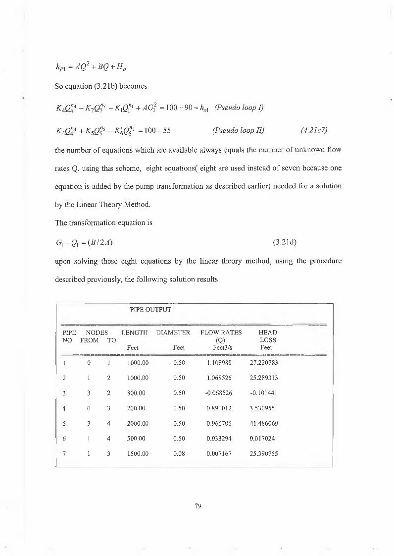
hP l = A Q 2 + B Q + H 0

So equation (3.21b) becomes

K4Q"4 - K 7Q"7 - K XQ*X + AG? = 100 - 90 - hol (Pseudo loop I)

K 4Q”< + K 5Q:”5 - K 'tQ l* = 100 - 55 (Pseudo loop I I) (4.2lc7)

the number of equations which are available always equals the number of unknown flow

rates Q. using this scheme, eight equations( eight are used instead of seven because one

equation is added by the pump transformation as described earlier) needed for a solution

by the Linear Theory Method.

The transformation equation is

Gl - Q l = ( B/ 2A) (3.2 Id)

upon solving these eight equations by the linear theory method, using the procedure

described previously, the following solution results :

PIPE OUTPUT

PIPENO

NODES FROM TO

LENGTH

Feet

DIAMETER

Feet

FLOW RATES(Q)

Feet3/s

HEADLOSSFeet

1 0 1 1000.00 0.50 1.108988 27.220783

2 1 2 1000.00 0.50 1.068526 25.289313

3 3 2 800.00 0.50 -0.068526 -0.101441

4 0 3 200.00 0.50 0.891012 3.530955

5 3 4 2000.00 0.50 0.966706 41.486069

6 1 4 500.00 0.50 0.033294 0.017024

7 1 3 1500.00 0.08 0.007167 25.390755

79

CHAPTER 4

Analysis and program Development

4.1 In troduction

The computer program described in this chapter is written to analyse steady state flows

and pressures for pipe distribution systems. The program can be applied to other liquids,

but does not generally apply to gas flow unless the assumption of constant density is

acceptable.

The program is written to accommodate any piping configuration and various hydraulic

components such as pumps, valves (including check valves), any component which

produce significant head loss (such as meters, bends, etc.) and pressure regulating valves.

Computations can be carried out using English units of CFS, GPM, or Standard

International (SI) units.

4 .2 Program A nalysis

This program is written to compute the flow rate in each pipe in the network and

therefore to compute the head loss in each pipe. To simplify the problem it is necessary to

describe the features of the piping system using data, which assigns numerical values to

the pertinent system characteristics. Part of this data refers to the physical characteristics

80

of the pipe system components and the rest to pressure and flow requirements imposed on

the system.

Before analysis, a network must be defined in terms of units such as pipes and pumps that

the program allows for.

4.2.1 Representation of Networks

This section includes a general description of pipe system configuration and pipe system

parameters which require data input.

£? Pipe system geometry

Pipe section

The principal element in the pipe system is the pipe section which of constant diameter

sections that can contain fittings such as bends, valves and pumps .

The end points of a pipe section are called nodes and are classified either as junction node

or fixed grade node.

Junction node

A node where two or three pipes meet or where flow is input in or removed from the

system.

81

If a pipe diameter change occurs at a component such as a valve or a pump, this point is a

junction node.

^ Real loop

A closed pipe circuit with no closed pipe circuits contained within it.

Pseudo loop

Which connects one reservoir to another one or to a source pump

Consequently such pseudo loops can always be defined, because at least two reservoirs

and /or pumps must exist in a network if all external flow rates are not known.

If the junctions, real loops, and the pseudo loops are identified as described above the

following holds for all pipe system: NP = NJ + NL

NP = number of pipes

NJ = number of junction

NL = number of loops

in which

NL = NLRcal + NPS

Where

NLRcal = no of real loops

NPS = no of pseudo loops

NPS = Nresenair + Npumps -1

N reservomr= »o of the reservoirs

Npumps = no of source pumps

82

0 Pipe System Components

Data regarding the physical characteristics of the components in the pipe system must be

obtained prior to making compute analysis.

A general description of the components, which are incorporated into the program and

the necessary data, follows:

• Pipe section

The total length, inside diameter and roughness of each pipe section must be input as

data. The designation of pipe roughness depends on the head loss equation used.

There are two major methods to compute the line losses:

a) H a z e n -W il l ia m e q u a tio n :

Because most users are primarily interested in water distribution, the Hazen William

equation, which was developed primarily for this purpose is normally used to compute

line losses.

The Hazen William equation is:

If this expression is to be employed, the roughness coefficient for this expression must be

input as data for each pipe .

This coefficient depends on the type of the condition of each pipe.

b) D a r c y - W e is b a c h e q u a tio n :

This expression can be applied to systems transporting water and other liquids other than

water. If this option is employed, the roughness for each pipe section corresponding to

the Darcy-Weisbach expression must be input as data as well as the kinematics viscosity

of the liquid for the system.

The Darcy -Weisbach equation is,

hr = f . LV2 2 gD

1 , OI , e 9.35.^ = 1 ,4 - 2 ,ogl, V ^ )

where

f = friction factor

Re = Reynolds number

e = roughness(ft)

84

• PUMPS:

A pump can be included in any line of the pipe system .The characteristics of pumps can

be described as follow.

0 Points of operating data.

Pump characteristics can usually be fitted approximately with a parabolic equation

An exponential curve can be fit to this data to obtain characteristic curve describing the

pump operation of the form:

hp = A Q 2+BQ + H0

in which A, B, and Ho are constants for a given pump and might be determined by fitting

lip to the three points taken from a pump characteristics curve using Least square method

[1,3] (see appendix A).

• Minor loss components

The head loss h, caused by a minor loss is proportional to the velocity head.

85

The loss coefficient K L is analogous to fL/D. In fact, some prefer to express loss

coefficient as an equivalent pipe length:

4.2.2 Algorithm for the solution of the linear theory method

Pipe network equations for steady state analysis have been commonly expressed in two

ways. Equation which express mass continuity and energy conservation in terms of the

discharge in each pipe section have been referred to as real loop and pseudo loop

equations. In terms of the unknown discharge in each pipe, a number of mass continuity

and energy equations can be written equalling the number of pipes in the system. For

each junction node a continuity relationship equating the flow into the junction to the

flow is written as:

! ( & ) ,„ - Z < £ ) . = c

in which C is the external flow at the junction (commonly called consumption or

demand). C is positive if flow is into the junction and negative if it is out from the

junction.

For each primary loop the energy conservation equation can be written for pipe sections

in the loop as follows:

i ,K iQ r =o

86

where K is a pipeline constant which is a function o f line length (L), diameter (D ), and

roughness e, or friction factor (/), and n is an exponent. The values o f K and n depend on

the energy loss expression used for the analysis.

For the f-Iazen-William equation

4.73 LK = ✓-.1.852 4.87^ HIV U

the exponent n=1.85.

For the Darcy-Weisbach equation

y Î1 2 gDA2

and the exponent n is in the range (1.85 to 2.0)

The minor loss in pipe section (hL)is given as

hL = - 2 —L * 2gA

where K,m is a function o f the sum o f the minor loss coefficients for the fitting in the pipe

section.

That is true for loops that do not include pumps, if there are pumps in the loop then the

energy equation states that the sum of the energy losses around the loop equals the energy

put into the liquid by a pump, or

+ r > e ! ±A,f 2 gDA 2 gDA

h, = ( Y — Æ . + Y — K-l t )Q 2 ± ( A Q 2 + B Q + I I 0) f 2 gDA 2gDA 6

87

The linear method is based on a simultaneous solution of the basic equations for the pipe

system. Since the energy equations for the loop equation s are non-linear these equations

are first linearized . This is done by approximating the head in each pipe as

The first step is to obtain K and n for the exponential formula , that is done by computing

the first value of K and n from the Hazen-William equation.

For the first iteration each K' is set to equal to K t , which is equivalent to setting all flow

rates Qi0 equal to unity [5,12,13,18,44].

Combining these artificial linear loop equations with the continuity equations provide a

system of n linear equations which can be solved by linear algebra.

The solution will not necessarily be correct because of Qiu ’s will probably not have been

estimated equal to the ’s produced by the solution. By repeating the process, after

improving the estimates to Qi ,eventually the Qi0 ’s will equal the Qi ’s, after the iteration

the corrcct solution has been obtained.

4 .3 C om puter program

The computer program is written in C language, to solve the basic pipe system

equations using the linear theory method .

Basically the program reads input data defining parameter values for each pipe and

pressure and flow specifications.

Several items should be noted about this program:

S different type of liquids are applied to the program

^ the basic equation used for the simulation is Darcy-Wcisback equation unless

otherwise specified

^ Unconditional number of trials allowed in the program and it is often depends on the

accuracy spec ill cation.

S The calculation continues until a relative accuracy of 0.0000001 is attained unless

otherwise specified.

The basic system equations are solved using spare matrix.

A complete listing of the C program including all functions (subroutines) is presented in

appendix B

89

4.3.1 Program algorithm

T h e m a jo r ta sk s p e r fo r m e d b y the p r o g r a m a r e th e fo l lo w in g

1 Determine type of operation to be performed and entering file name, there is a list of

choice to choose such as display the existing file or exit the program.

2 Read the input data that defines the network.

3 Develop from this information the system of Q-equations, i.e., the junction continuity

equations and the energy equation around pseudo and real loops of the network.

4 Make use of the linear theory method to transform the non-linear energy equation into

linear equations as described earlier. Set up the arrays and solve the simultaneous

linear equations using Gauss elimination method.

5 Obtains the head loss at each pipe after the pipes flow rates have been found.

6 Write the solution results in tables that can be readily understood.

90

4.3.2 Program Variables

The data requirements for the program are as follows:

Input variables

Detailed instructions on the preparation of input data are as follow:

□ System input data requirement

The input data for the system to solve the network equations are as follow

a) the type of equation will calculate the head loos friction(Type)

i. if the Darcy-Weisback equation is used Type— 1

ii. if the Hazen-Williams equation is used Type— 2

b) after the programmer indicates the type of equation to calculate the head friction

losses, the program require the network elements to be read in. The network elements

variables are as follow

1) The number of pipes in the network, NP (int NP) which indicates how many pipe

in the network.

2) The number of junctions in the network, NJ (int NJ) which indicate how many

junctions in the network.

3) the number of real loops in network, NL (int NL) .If the network is branching

network .i.e. there is no closed loops in the network the user must read in the NL

equal to 0

4) If the network contains pumps, the program requires to read in how many pumps in

the network, NPUMP (int NPUMP).

91

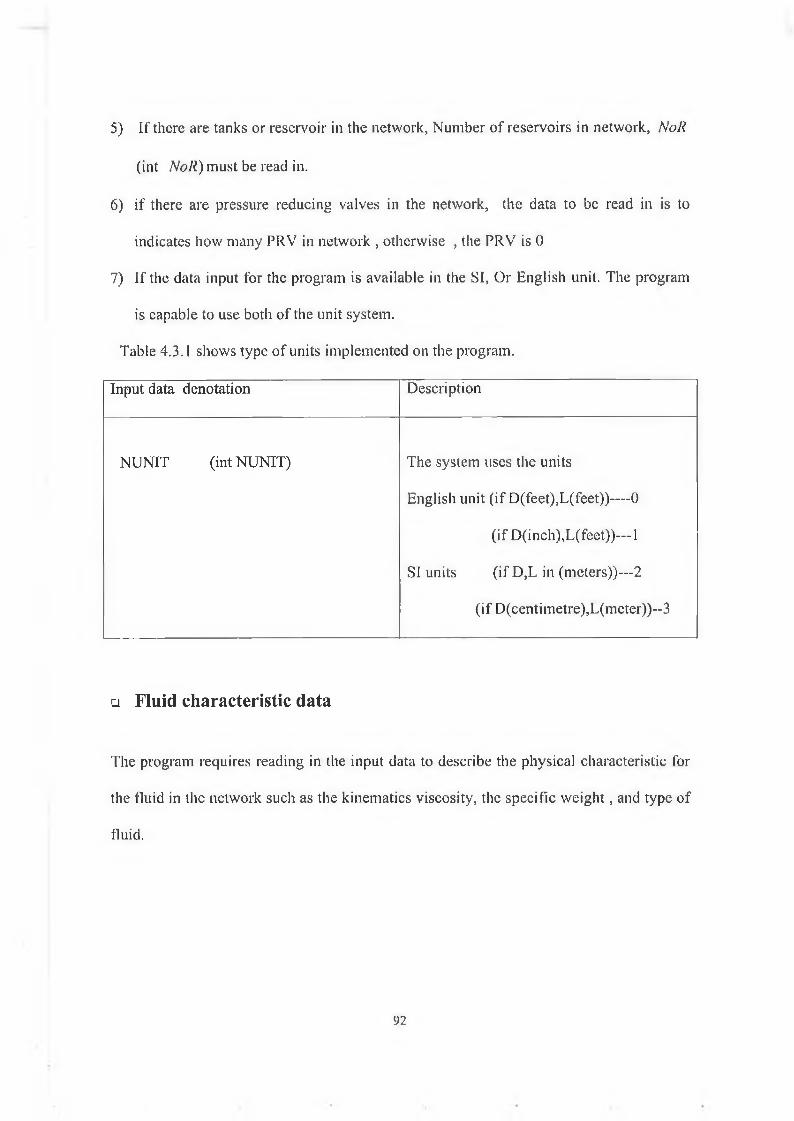
5) If there are tanks or reservoir in the network, Number of reservoirs in network, NoR

(int NoR) must be read in.

6) if there are pressure reducing valves in the network, the data to be read in is to

indicates how many PRV in network , otherwise , the PRV is 0

7) If the data input for the program is available in the SI, Or English unit. The program

is capable to use both of the unit system.

Table 4.3.1 shows type of units implemented on the program.

Input data denotation Description

NUNIT (intNUNIT) The system uses the units

English unit (if D(feet),L(feet))— 0

(if D(inch),L(feet))—1

SI units (if D,L in (meters))—2

(if D(centimetre),L(meter))-3

□ Fluid characteristic data

The program requires reading in the input data to describe the physical characteristic for

the fluid in the network such as the kinematics viscosity, the specific weight, and type of

fluid.

92

□ Pipe data

For each pipe in the network, every pipe is given pipe number, diameter, length, and

roughness. The roughness may be either the equivalent sand roughness e (in the same

units as the pipe diameter) for use in the Colebrook-White and Darcy-Weisback

equations, or a Hazen-Williams CIIW. If the pipe include any minor loss device, the

value of minor loss coefficient is required to be read in.

□ Junction data

For each junction in the network, each junction is given junction number. The input data

required to describe every junction.

They arc as follows:

1- First, if there is a demand at the junction, there are four options the read in the

demand in terms of unit. For example, if the demand in cubic feet per second the

option is available by indicating the demand in CFS

2- If the demand leaves the junction, a minus sign is given, and a positive sign if the

opposite.

3- Number of pipes around the junction, and a list of these pipe numbers with a minus

sign if the flow is from the junction. These information are used to define the

junction continuity equations.

93

□ R e a l lo o p d a t a

For every real loop (closed loop) in the network, the number of pipes in that loop, and a

list of these pipes must be entered. A negative sign must precede the pipe number if the

direction around the loop opposes the assumed direction of flow in the pipe.

□ P s e u d o lo o p d a t a

The pseudo loop is a loop with no flow pipe, which connects reservoirs. The program

will compute how many pseudo loops are needed for the network.

It the responsibility of the user to decided which path to suggested connecting the

reservoirs.

For every pseudo loop in the network, the number of pipes in the suggested path, and a

list of these pipes must be read in. A negative sign must precede the pipe number if the

direction around the loop opposes the assumed direction of flow in the pipe.

In addition, the data for the pseudo loop contains the elevation of each reservoir

□ P u m p d a t a

For each pump in the network if they exist, the number of the pump , and the

description of the operation data for the pump are needed.

If the pump is described by performance data, a list of the three points describing the

(Q, hp) is needed. The program makes use of the least square method to define these

data into the form of quadratic equation of the form

hp = AQ2 +BQ + H0

94

4.3.3 Program Structure

The structure chart of the program is as shown in Figure (4.1)

The program is divided into the following functions:

1 )Main ( ) This function determines the type of operations to be performed and calls

the appropriate computational functions, and displays a list of choice whether to

show all the inputs or to print out the result of the program.

2)Input (). Read in the network parameters such as number of pipes in the network,

number of junctions, the system unit which has been used, the type of equations

used to define the friction losses, and the number of loops. This function stores and

writes these data to an input file, which can be very useful for updating the data for

the network if that is necessary. Figure (4.2) shows the structure of this function.

3) Output () . This function reads in the data for the network from the input file. Also

this function prints the result of the program after calling .This function has two

sub-function. Figure (4.3) and Figure (4.4) shows the structure,

a) Linear Darcy ( ). If the Darcy-Weisbach equation is used, this function will be

called. This function will set up the mass continuity, loops equations as arrays, and

solve the simultaneous linear equations using Gauss elimination method. This

function computes the flow rates of each pipe in the network based on the use of

Darcy-Weisbach equation for computing the friction loss. Figure (4.4) shows the

structure of this function.

95

b) Linear_Hazen_William ( ) If the Hazen-William equation is used, this function will

be called. This function computes the flow rates of each pipe in the network based

on the use of Hazen-William equation for computing the friction loss.

4)Gauss_elimination ( ) This function solves the system of equations [A]{X}-{B}

using the Gauss elimination method with partial pivoting. This subroutine will be

discussed in details in appendix (A).

5)Newton_Raphson (). This function computes the roots of an equation of the form

f(x )=0 using the Newton-Raphson method, i.e. computes the value of the friction

factor f This program will be discussed in details in appendix (A).

6) f( ). The main purpose of this function is to return the value of a function f(x )

evaluated at jc. This function is called by function Newton_Raphson ( ) .

7) df( ). Returns the value of derivative of the function f(x). This function is called as

well by the function NewtonJRaphson ().

8) -poly Jeastsqr (). If a pump exist in the network, and its characteristic is described by

performance operating data, this function is invoked to fit the curve for the

operating data using least square method (see appendix A).

96

Figure 4.1 structure fo r the computer program

Pipe network definition Understand the problem statement. Ì

I Y I a i n ( )

Ti

Output ( )Out put fo r an existing file J I n p u t ( )

C r e a t e a n e w i n p u t f i l e

Type o f formula used to calculate head lossesDarcy or Hazen-W illiam equations

11

Yes

97

Figure 4.2 structure o f function Input ( )

Pipe (lataJA[),JB[J (nodes conned l lie pipe)D(d iam tler), L( length)E( Relative roughness) KL(minor loss coef)

Type oi equation used to compute iiead losses Darcy-Weisback or Hazen-Williams

Network definition NP,NJ,NL,NPUMP,NOR

Loops dataNumber o f pipes in the loop,elevation o f the reservoir connecting the paths

Junctions dataN u m b e r o f p i p e a r o u n d t h e

j u n c t i o n ,

D e m a n d u t t h e j u n c t i o n

E l e v a t i o n o f t h e j u n c t i o n

Figure 4.3 structure o f function O u tp u t ( )

I

Figure 4.4 structure for the function Linear_Darcy ( )

Linear _Darcy ( )

JInitialise KP[] fo r each pipeKP[i]=0.00093517*L[i]/pow(D[i],4.87) (E S UNITS) KP[i]=0.002I2*L[i]/pow(D [i],4.87) ( S I U NITS) J

(Write the mass continuity equation Around each junction

Z e , ± c = o IWrite the energy equation around each Real loops

^K,Qf±XhP=0

Write the energy equations around each pseudo loops

Y.K,QT ±5> = &H

rTransform the non-linear energy equation into linear equation by approximating

h r = [k .Qo r ' f c , . = K.-Q,

Call Gauss elimination ( ) l- M-To sove the set o f equation [A] W = [B ]

No iteration<l

<

Call Newton_Raphson ( )To compute a and b fo r the friction

f a c t o r _____________________

Compute m odified K ’ new

aL [¡']K P \ i

J

100

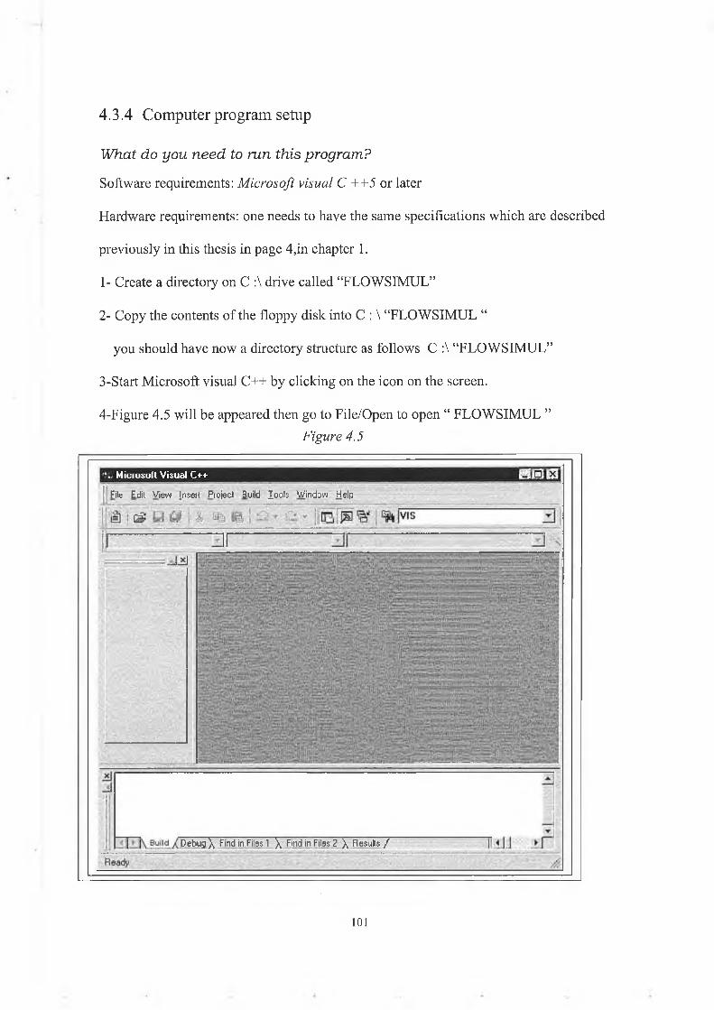
What do you need to run this program?

Software requirements: Microsoft visual C ++5 or later

Hardware requirements: one needs to have the same specifications which are described

previously in this thesis in page 4,in chapter 1.

1- Create a directory on C :\ drive called “FLOWSIMUL”

2- Copy the contents of the floppy disk into C : \ “FLOWSIMUL “

you should have now a directory structure as follows C :\ “FLOWSIMUL”

3-Start Microsoft visual C++ by clicking on the icon on the screen.

4-Figure 4.5 will be appeared then go to File/Open to open “ FLOWSIMUL ”Figure 4.5

4.3.4 Computer program setup

Microsoft Visual C++

File Edit View Insert Pioject Build lools Window Help

Debug X Find in Files 1 \ Find in Files 2 \ Results/

101

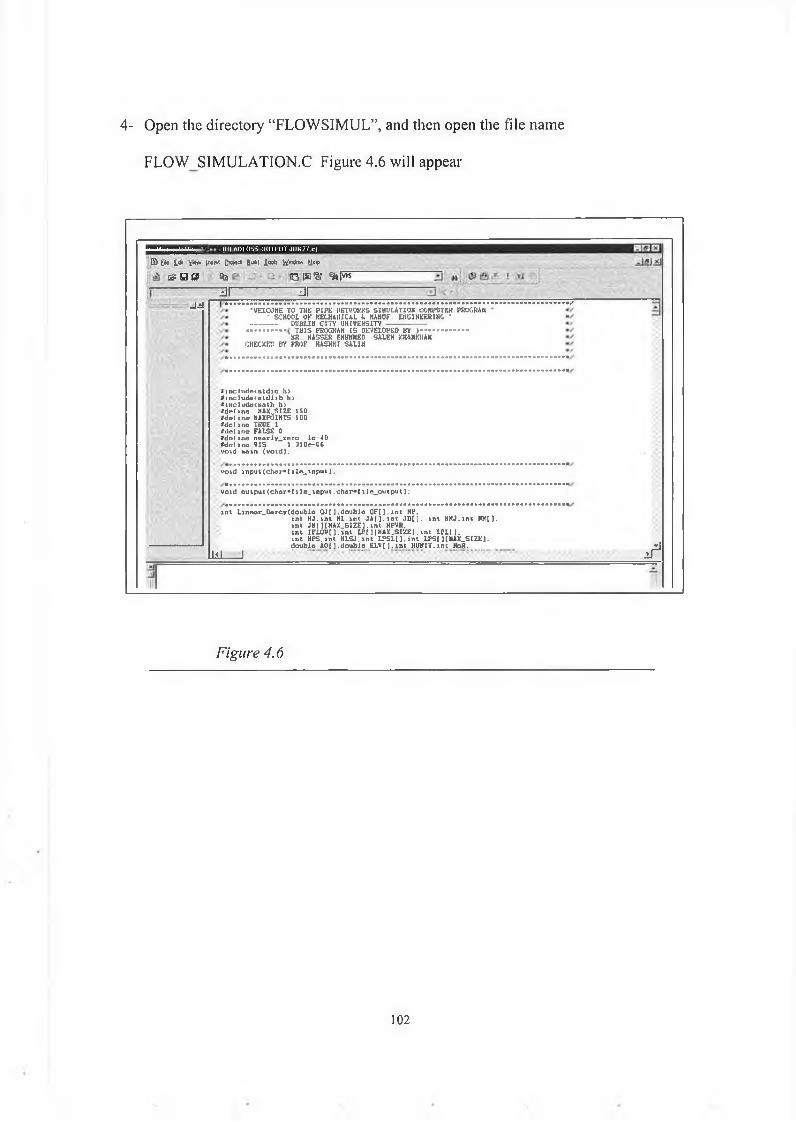
4- Open the directory “FLOWSIMUL”, and then open the file name

FLOW SIMULATION.C Figure 4.6 will appear

- IHEADLOSS-OUIPUT JUN27.c|

(3 E h idi I * * ' |m nt £rty)d fiofcf X « * WpdOW H rp

s u o ia OlB f 'fcl'fls-

_l.iln r “□r

•UEICOBE TO T1IE P IPE IIETI'ORKS SIHUU TIOII COMPUTES PROGRAK • SCM001 OS' IIECHAIIICAL (. KAtlUF BIOIHKERIIIG •----- DUB1I1I CITY UllIVESSm-------

t h i s PROGRAM £S DEVKOPED BY >............................MR HASSER EMHHMED SALEH KIIAHKHA11

CHECKED BY FROf HASHtil SAUH

i tnciudotatdio h> *tnc!utJe<sldlib h> s inelude<aath h>Jdefinr MAX..SIZE ISOi d e i m i» HAXPOIMTS 100/dei i nc TRUE 1/ d e f i n e FALSE 0id o l i n e n e o r iy _ r o r o l e - 4 0/ d r l i n c VIS 1 . 3 1 0 e -0 6void *oin (void).

v o id i n p u t ( c h o r " ! i l e _ i n p u t ) .

v o id o u t p u t ( c h a r » t l l e _ i n p u t . c h o r « t l l e _ o u t p u t ) ;

m t L in c « r _ B a rc y ( d o u b le O J l J .d o u b lo G F U . i n t HP.i n t M J . in t ML. m t J A ( ] . i n t JDJ ] . i n t H H J .m t HM[J. l n t J N lK H A X _ S IZ E J .in i WPVR. i n t IF L O W IJ .in t IP [] (H A X _ S IZ E ] ,in t 1 F 1 1 J . m e M P S .in t H L S J .in t IF S K [ ] .* M L PS[)(X A X _SIZ E ]. d o u b le A O [J .d o u b le E L V ( J . in t H U N IT .in t HoR.

LlL i f1

Figure 4.6

102

6-Run the program by clicking on the compile icon (F7) to check if there is any logical

error

6- Execute the program by clicking on the icon execute (F8)

7- Figure (4.7) will appear on the screen

The main menu will give you 3 options

a) create new data

b) show the out put for an existing file

c) exit the program

9- If your choice is (a) or (b) then

a) enter name for the file input to read in all the data requirements

b) enter name for the file output to show the result

'■’s HEADLOSS-OUTPUT- JUN27

A uto a l tel M f f j s a J

HA IN MENU1 - C rea te a new in p u t f i l e o r u p t a t e an e x i s t i n g i n p u t f i l e2 - shows l i s t of c o n te n t s of th e o u tp u t f i l e3 - E x i s t the program your ch o ice <1*2 o r 3>?1

E n te r th e f i len am e of th e in p u t f i l e

Figure 4.7

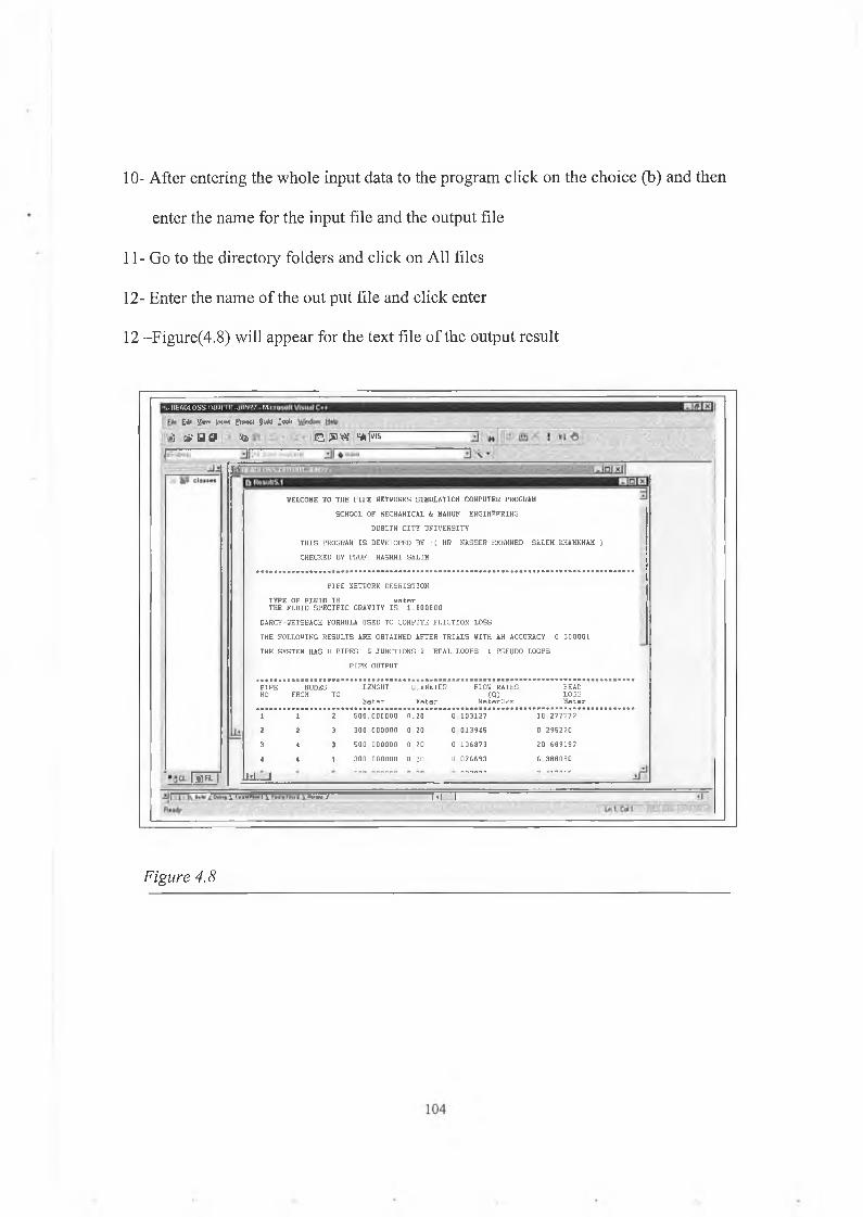
10- After entering the whole input data to the program click on the choice (b) and then

enter the name for the input file and the output file

11- Go to the directory folders and click on All files

12- Enter the name o f the out put file and click enter

12 -Figure(4.8) will appear for the text file o f the output result

.. HE ADt OSS-OUTPUT JUM2/ - Mtr.£<Ji V o» JweS gWKil gufcl l « i i

ii » 'B 9 lb C PB® f fm(j !

la».

WELCOME TO THE PIPE NETWORKS SIMULATION COMPUTER PROGRAM SCHOOL OF MECHANICAL it MANUF ENGINEERING

DUBLIN CITY UNIVERSITY THIS PROGRAM IS DEVELOPED BY :( HR NASSER EMHMHED SALEM KHAHKHAH ) CHECKED BY PROF HASHMI SALIM

PIPE NETWORK DESRIBTIONTYPE OF FLUID IS waterTHE FLUID SPECIFIC GRAVITY IS 1.000000

DARCY-WEISBACH FORMULA USED TO COMPUTE FRICTION LOSSTHE FOLLOWING RESULTS ARE OBTAINED AFTER TRIALS VITH AH ACCURACY 0.000001 THE SYSTEM HAS 0 PIPES 5 JUNCTIONS 2 REAL LOOPS 1 PSEUDO LOOPS

PIPE OUTPUT

PIPEWO

NODES FROH TO

LEHGHTMeter

DIAMETERMeter

FLOW RATES(Q)Meter3/s

HEAD LOSS He ter

1 1 2 500.000000 0,20 0 103127 10 2773722 2 3 300.000000 0.20 0 013945 0 2952203 4 3 500 000000 0 20 0 106873 20 6891974 4 1 300 000000 0 20 0 076693 6 388000

id I

1 i;.i*r“ rry ¡Mimi/ T i l l 1

Figure 4.8

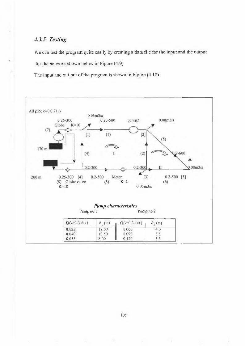
We can test the program quite easily by creating a data file for the input and the output

for the network shown below in Figure (4.9)

The input and out put of the program is shown in Figure (4.10).

4.3.5 Testing

All pipe e=0.0.21m0,03m3/s

0.25-300 0.20-500 pump2 0.08m 3/s

(8) Globe valve (3) K=2 (6)K=10 0.05m3/s

Pump characteristicsPump no 1 Pump no 2

Q fm 3 / s e c ) hp 0») Q f m V s e c ) hp (m)

0.025 12.00 0.060 4.00.040 10.50 0.090 3.80.055 8.00 0.120 3.5

105

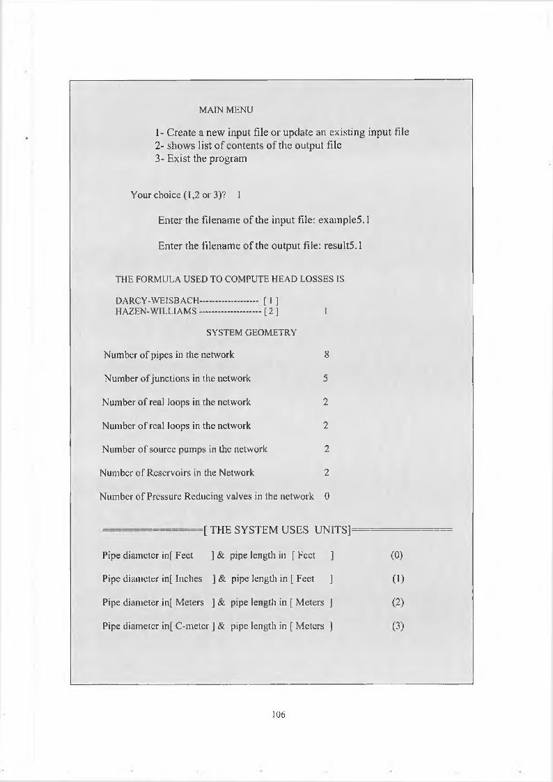
MAIN MENU

1- Create a new input file or update an existing2- shows list o f contents o f the output file3- Exist the program

input file

Your choice (1,2 or 3)? 1

Enter the filename o f the input file: examples. 1

Enter the filename o f the output file: result5.1

THE FORMULA USED TO COMPUTE HEAD LOSSES IS

DARCY-WEISBACH.............................. [ 1 ]HAZEN-WILLIAMS................................ [ 2 ] !

SYSTEM GEOMETRY

Number of pipes in the network 8

Number of junctions in the network 5

Number of real loops in the network 2

Number of real loops in the network 2

Number of source pumps in the network 2

Number of Reservoirs in the Network 2

Number of Pressure Reducing valves in the network 0

f TT-TT2 OV'CT'CN/f ITCHC T IXI XT’ClL 11 i l i à i o 1 L IVI U jL /O U IN 11 j j

Pipe diameter in[ Feet ] & pipe length in [ Feet ] (0)

Pipe diameter in[ Inches j & pipe length in [ Feet ] ( 0

Pipe diameter in[ Meters ] & pipe length in [ Meters ] (2)

Pipe diameter in[ C-meter ] & pipe length in [ Meters ] (3)

106

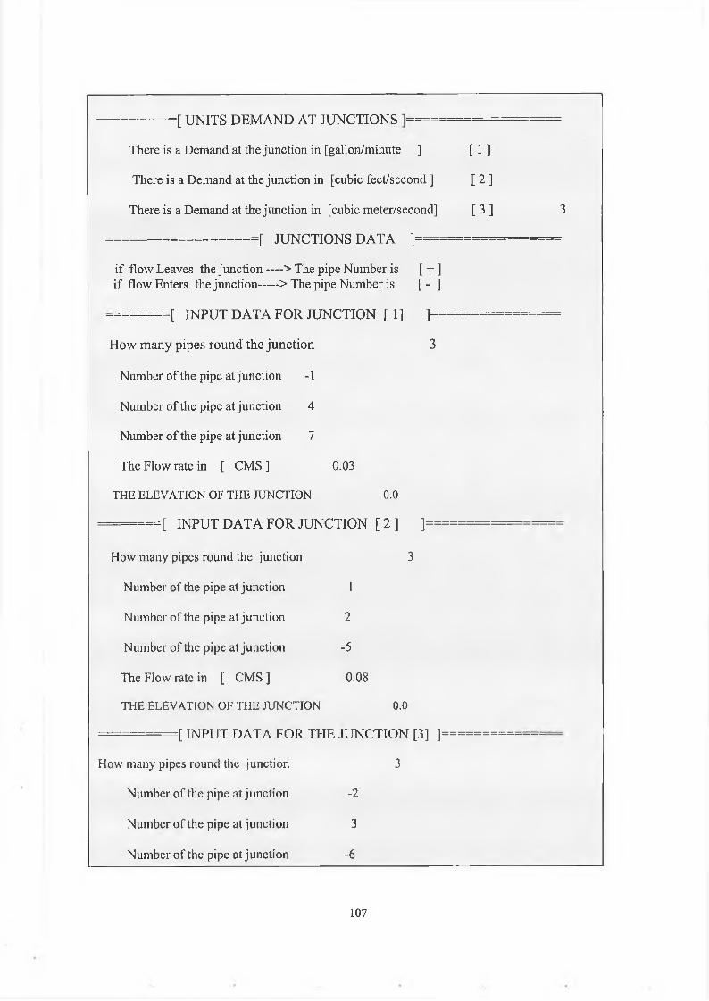
There is a Demand at the junction in [gallon/minute ] [ 1 ]

There is a Demand at the junction in [cubic feet/second ] [ 2 ]

There is a Demand at the junction in [cubic meter/second] [ 3 ] 3

_ _ = = _ [ JUNCTIONS DATA ] = = — — —

if flow Leaves the junction — > The pipe Number is [ + ]if flow Enters the junction > The pipe Number is [ - ]

=— [ INPUT DATA FOR JUNCTION [ 1] ]— = —

_ = _ [ UNITS DEMAND AT JUNCTIONS

H o w m a n y p ip e s ro u n d th e ju n c t io n 3

N um ber o f the p ipe at ju n ction -1

N um ber o f the p ipe at ju n ction 4

N um ber o f the p ipe at ju n ction 7

The F lo w rate in [ CMS ] 0 .03

THE ELEVATION OF THE JUNCTION 0.0

— = = . [ INPUT DATA FOR JUNCTION [ 2 ] ] =

H ow m any pipes round the jun ction 3

N um ber o f the pipe at ju n ction 1

N um ber o f the pipe at junction 2

N um ber o f the pipe at jun ction -5

T he F low rate in [ CMS ] 0 .08

THE ELEVATION OF THE JUNCTION 0.0

------------ [ INPUT DATA FOR THE JUNCTION [31 ] =

H ow m any p ipes round the ju n ction 3

N um ber o f the pipe at ju n ction -2

N um ber o f the p ipe at junction 3

N um ber o f the pipe at junction -6

107

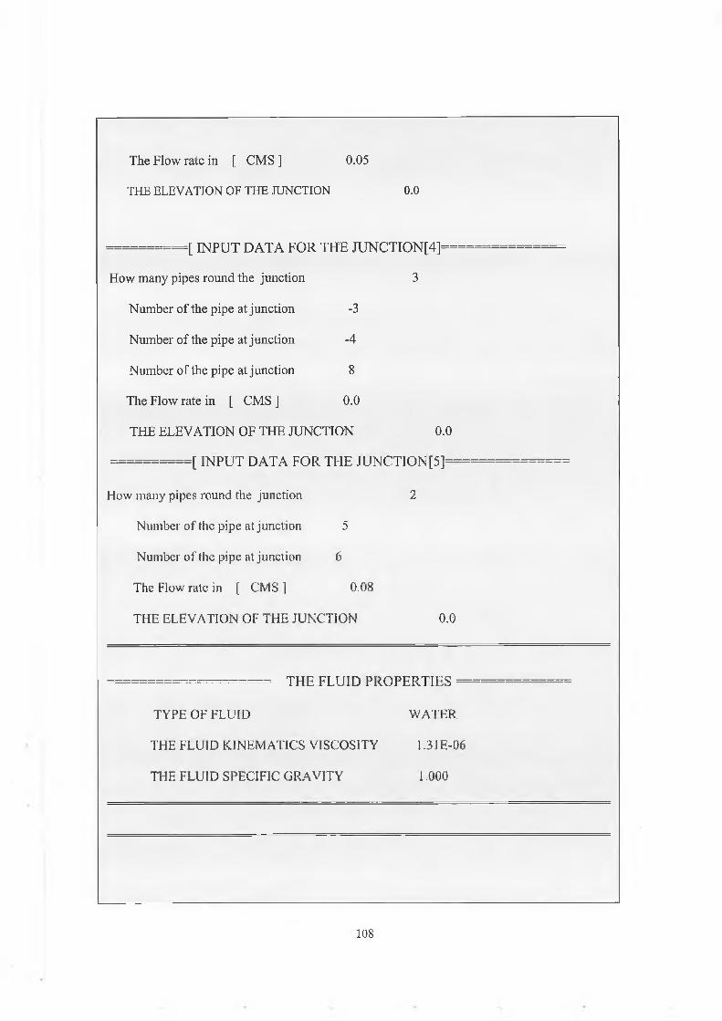
THE ELEVATION OF THE JUNCTION 0.0

The Flow rate in [ CMS ] 0.05

=[ INPUT DATA FOR THE JUNCTION[4]=

How many pipes round the junction 3

Number of the pipe at junction -3

Number of the pipe at junction -4

Number of the pipe at junction 8

The Flow rate in [ CMS ] 0.0

THE ELEVATION OF THE JUNCTION 0.0

■ ----------[ INPUT DATA FOR THE JUNCTION[5]=

How many pipes round the junction 2

Number of the pipe at junction 5

Number of the pipe at junction 6

The Flow rate in [ CMS ] 0.08

THE ELEVATION OF THE JUNCTION 0.0

= = = = = = = THE FLUID PROPERTIES =

TYPE OF FLUID WATER

THE FLUID KINEMATICS VISCOSITY 1.31E-06

THE FLUID SPECIFIC GRAVITY 1.000

108

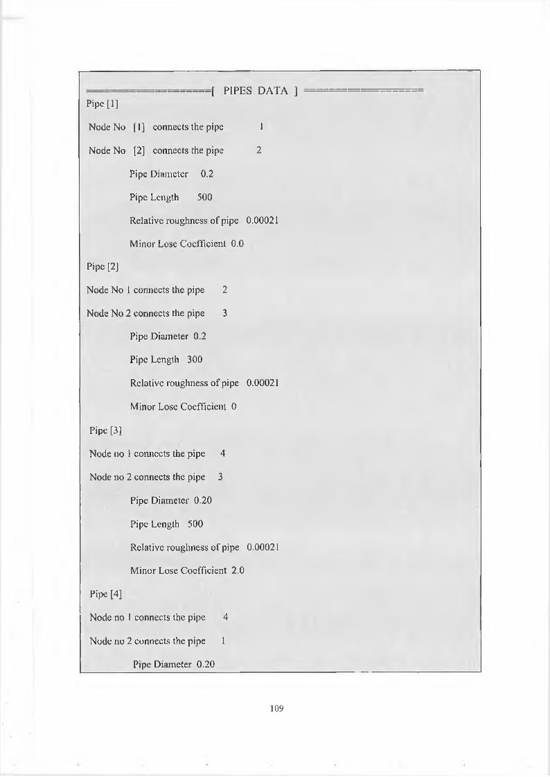
r n i n r c r* A T A 11 r X r H o U A 1 A J

Pipe [1]

N o d e N o [1] con n ects the pipe 1

N od e N o [2] con n ects the p ipe 2

Pipe D iam eter 0 .2

Pipe Length 500

R elative roughness o f p ipe 0 .00021

M inor L ose C oeffic ien t 0 .0

Pipe [2]

N o d e N o 1 con n ects the pipe 2

N od e N o 2 con n ects the p ipe 3

Pipe D iam eter 0 .2

Pipe Length 3 0 0

R elative roughness o f p ipe 0 .00021

M inor L ose C oeffic ien t 0

Pipe [3]

N od e no 1 con n ects the pipe 4

N o d e no 2 con n ects the pipe 3

Pipe D iam eter 0 .2 0

Pipe Length 500

R elative rou gh ness o f p ipe 0 .00021

M inor L ose C o effic ien t 2 .0

Pipe [4]

N od e no 1 con n ects the p ipe 4

N o d e no 2 con n ects the p ipe 1

Pipe D iam eter 0 .2 0

109

R elative roughness o f p ipe 0 .00021

M inor L ose C oeffic ien t 0 .0

N od e no 1 con n ects the pipe I

N od e no 2 con n ects the p ipe 5

Pipe D iam eter 0 .2 0

Pipe Length 600

R elative roughness o f p ipe 0 .00021

M inor L ose C oeffic ien t 0 .0

Pipe [6]

N od e no 1 con n ects the pipe3

N o d e no 2 con n ects the pipeS

Pipe D iam eter 0 .2 0

P ipe L ength 500

R elative rou gh ness o f pipe 0 .0 0 0 2 1

M inor L ose C o effic ien t 0 .0

Pipe [7]

N od e no 1 con n ects the pipeO

N od e no 2 con n ects the p ip el

Pipe D iam eter 0 .25

Pipe Length 300

R elative rou gh ness o f p ipe 0 .0 0 0 2 1

M inor L ose C o effic ien t 10

Pipe Length 300

Pipe [5]

110

N od e no 1 con n ects the pipeO

N o d e no 2 con n ects the pipe4

Pipe D iam eter 0 .25

Pipe Length 300

R elative roughness o f pipe 0 .00021

M inor L ose C oeffic ien t 10

------------------- INPUT DATA FOR THE REAL LOOPS ---------------

The d irection o f the loop a lw ays is * * * C lo ck w isc* * * *

I f the direction o f the flow in the pipe C lo c k w is e --------- [+]

If the d irection o f the flow in the p ipe a n ti-C lock w ise— [-]

-------------------INPUT DATA FOR THE REAL LOOP [ 1 ] = = —

H ow m any p ipes in the Real loop [ 1 ]5

the num ber o f the p ipe in the lo o p l

the num ber o f the pipe in the loop -2

the num ber o f the p ipe in the loop-3

the num ber o f the p ipe in the loop 4

the num ber o f the pipe in the loop -9

=============== INPUT DATA FOR THE REAL LOOP [ 2 ] ====

H o w m an y p ip es in the R eal loop [ 2] 3

the num ber o f the pipe in the loop 5

the num ber o f the pipe in the loop -6

the num ber o f the p ipe in the loop 2

Pipe [8]

111

= ---------- — [ DATA FOR RESERVOIRS ] = —

Enter the Reservoir elevation which connected to pipe [7 ] 170

Enter the Reservoir elevation which connected to pipe [8 ] 200

=[ INPUT DATA FOR PUMPS ]=

= = _ [ INPUT DATA FOR PUMP [ 1 ] ] = = —

Enter the pipe number contains the pump 1

type of the operator for the pumptype of pump data :([1]—> operating data

:([2]—> performance operating data 2

Form ing the transform ation equations for the pum ps in the form -Q + G = B /2 A

the sign [ - ] g o es w ith the p ipe num ber the sign [ + ] g o e s w ith the num ber o f the pum p

the num ber o f the p ipe in the loop -1

the number of the pipe in the loop 9

The pump is described by perform ance operating data d egree o f p o lyn om ial 2

num ber o f data points 3

enter x [ l] ;0 .0 6 0

enter y[ 1 ];4 .0

enter x [2 ];0 .0 9 0

enter y [2 ];3 .80

enter x [3 ] ;0 .120

enter y [3 ];3 .5

The co e ffic ien ts o f the best-fit po lynom ial are

a( 1) = 4 .1 0 0 0 0 0 a ( 2 ) = 1 .666667 a(3) = -5 5 .5 5 5 5 5 6

112

= = = = [ INPUT DATA FOR PUMP [ 2 ] ]

Enter the pipe number contains the pump 7

type of the operator for the pumptype of pump data :( [1]—> operating data

:([2]—> performance operating data :([3]—> useful horse power 2

Forming the transformation equations for the pumps in the form -Q+G=B/2A

the sign [ - ] goes with the pipe numberthe sign [ + ] goes with the number of the pump

the number of the pipe in the loop -7

the number of the pipe in the loop 10

the pump is described by performance operating data degree of polynomial 2 number of data points 3

enter x[l];0.025

enter y[l];12.00

enter x[2];0.040

enter y[2]; 10.50 enter x[3];0.055

enter y[3];8.00

the coefficient o f the best fit polynomial are a (l)= 12.277778 a(2) = 44.444444 a(3) = -2222.222222

113

The Network needs [1] pseudo loops

= = [ D A T A FOR PSEUDO LOOPS]— — = = = — ========

— = [ DATA FOR PSEUDO LOOP [ 1 ] ] _ _ _ _

Suggest a path to connect the two reservoir for pseudo loop [1]

If the path contains a pump [sign the pump by Np+1] (+ )-. if the flow in .the direction of the pipe which contains the pump in the direction of the path

How many pipes in the path 4

[ + ] if flow in the same direction of the energy line

[ - ] if flow opposite the energy line direction

the number of the pipe in the loop 7

the number of the pipe in the loop -4

the number of the pipe in the loop -8

the number of the pipe in the loop -10

DO YOU WANT TO ENTER MORE DATA- Y/N?

MAIN MENU

I - Create a new input file or update an existing input file2- shows list of contents of the output file3- Exist the program

your choice (1,2 or 3)?2

Enter the filename of the input file :example5.!

Enter the filename of the output file :result5.1

114

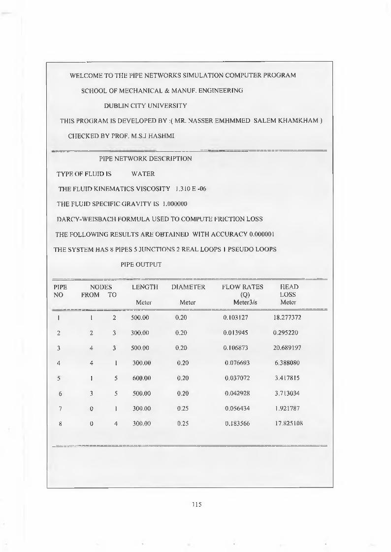
WELCOME TO THE PIPE NETWORKS SIMULATION COMPUTER PROGRAM

SCHOOL OF MECHANICAL & MANUF. ENGINEERING

DUBLIN CITY UNIVERSITY

THIS PROGRAM IS DEVELOPED BY ;( MR. NASSER EMHMMED SALEM KHAMKHAM )

CHECKED BY PROF. M.S.J HASHMI

PIPE NETWORK DESCRIPTION

TYPE OF FLUID IS WATER

THE FLUID KINEMATICS VISCOSITY 1.310 E -06

THE FLUID SPECIFIC GRAVITY IS 1.000000

DARCY-WEISBACH FORMULA USED TO COMPUTE FRICTION LOSS

THE FOLLOWING RESULTS ARE OBTAINED WITH ACCURACY 0.000001

THE SYSTEM HAS 8 PIPES 5 JUNCTIONS 2 REAL LOOPS I PSEUDO LOOPS

PIPE OUTPUT

PIPENO

NODES FROM TO

LENGTH

Meter

DIAMETER

Meter

FLOW RATES(Q)

Meter3/s

HEADLOSSMeter

I I 2 500.00 0.20 0.103127 18.277372

2 2 3 300.00 0.20 0.013945 0.295220

3 4 3 500,00 0.20 0.106873 20.689197

4 4 1 300.00 0.20 0.076693 6.388080

5 1 5 600.00 0.20 0.037072 3.417815

6 3 5 500.00 0.20 0.042928 3.713034

7 0 1 300.00 0.25 0.056434 1.921787

8 0 4 300.00 0.25 0.183566 17.825108

115

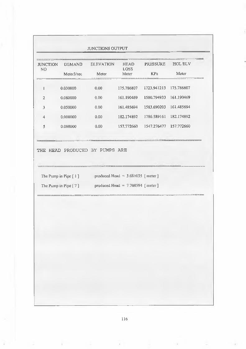
JUNCTIONS OUTPUT

JUNCTIONNO

DEMAND

Meter3/sec

ELEVATION

Meter

HEADLOSSMeter

PRESSURE

KPa

HGLELV

Meter

I 0.030000 0.00 175.786807 1723.941213 175.786807

2 0.080000 0.00 161.190469 1580.794933 161.190469

3 0.050000 0.00 161.485694 1583.690203 161.485694

4 0.000000 0.00 182.174892 1786.589161 182.174892

5 0.080000 0.00 157.772660 1547.276477 157.772660

TH E H EAD PR O DUCED BY PU M PS AR E

The Pump in Pipe [ 1 ] produced Head = 3.681035 [ meter]

The Pump in Pipe [ 7 ] produced Head = 7.708594 [ meter ]

116

CHAPTER 5

Results and Discussion

In order to illustrate the simulation of pipe networks using the linear theory method,

several examples will be presented here with their results, and will be compared with

other results that implemented different method of analysis.

First of all, the computer program is shown in appendix (B). Several computer programs

have been written in the past few years, and every program uses a different approach for

the method. What can be seen here is that the linear theory method has been used to

analyze the pipe network. In addition the method used here is based on the Jeppson

[12,13,18,44] approach.

Wood [17] had written a computer program based on the linear theory method, but his

method of approach has a few disadvantages, although it converges very rapidly. One of

these disadvantages is that the algorithm used in the simulation requires an initial guess

and that might cause problems if the initial guess was not close enough to the real flow

rate.

The first section of this chapter will implement the simulation on different samples of

pipe networks. To use the computer program several different types of information are

required.

117

First, the number of pipes, number of junctions, and number of loops in the network plus

other specifications such as denoting type of unit( i.e. ES or SI), number of allowable

iterations, viscosity of the fluid ,etc.

Second, data given the diameters, length, and wall roughness for each pipe. Third,

information for establishing junction continuity equations. This information is provided

by data input for each junction which contains the pipe numbers meeting at the junction.

If the assumed direction of flow is into the junction this number preceded by a minus.

Also if external flow occurs at the junction we must consider it as part of the junction

input data. Finally, information is required for the energy equations for each loop in the

network. For each loop in the network information data is provided to list the pipe

numbers in that loop, a minus proceeds the pipe number if the assumed direction of flow

is counterclockwise around the loop.

118

Consider this simple 6-pipe, 5-jnuction network shown below. This network is a one-loop

network.

Exam ple 5 .1

All e=0.005"All D in Inch and L in feet

Figure 5.1.A Small 6-pipe, 5-node network [13]

119

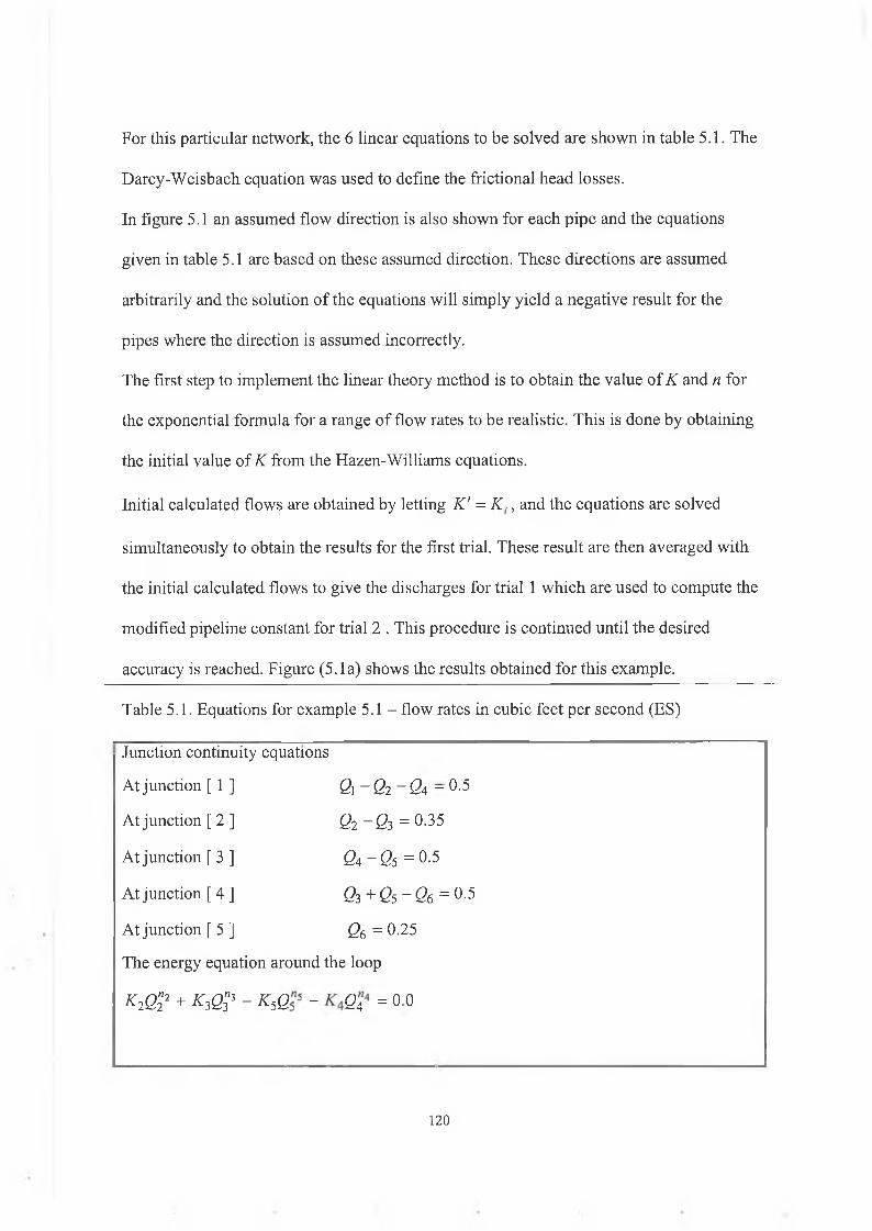
For this particular network, the 6 linear equations to be solved are shown in table 5.1. The

Darcy-Weisbach equation was used to define the frictional head losses.

In figure 5.1 an assumed flow direction is also shown for each pipe and the equations

given in table 5.1 are based on these assumed direction. These directions are assumed

arbitrarily and the solution of the equations will simply yield a negative result for the

pipes where the direction is assumed incorrectly.

The first step to implement the linear theory method is to obtain the value of K and n for

the exponential formula for a range of flow rates to be realistic. This is done by obtaining

the initial value of K from the Hazen-Williams equations.

Initial calculated flows are obtained by letting K' = K ., and the equations are solved

simultaneously to obtain the results for the first trial. These result are then averaged with

the initial calculated flows to give the discharges for trial 1 which are used to compute the

modified pipeline constant for trial 2 . This procedure is continued until the desired

accuracy is reached. Figure (5.1a) shows the results obtained for this example.

Table 5.1. Equations for example 5.1- flow rates in cubic feet per second (ES)

Junction continuity equations

At junction [ 1 ] Q\ - 02 -0 4 ~ 0.5

At junction [ 2 ] 02-03=0-35

At junction [ 3 ] 04-05=0.5

At junction [ 4 ] 03 + 05 - 06 = 0-5

At junction [ 5 ] 06 = 0.25The energy equation around the loop

K2Q? + K,Q? - KSQ -

o©IIcST

120

Analyzing the results from Figure (5.1a), leads to the following observations.

The relationship between the kinematic viscosity and the flow rates in pipes is

established. In this example methanol was applied on the network to compute the flow

and head losses at various temperatures. From Figure (5.1b) one can notice that the flow

rate is increased when the kinematic viscosity of the fluid is decreased.

From Figure (5.1c) the head losses in the pipes are increased when the flow rate

increases.

The relation between the head losses at junctions and the hydraulic grade line is always

linear, this is the same for pressure at the junctions as shown in Figure (5. Id, 5.1e).

To see how the changing of the demand at junction affects on the calculation of the head

losses at junctions, different value of demand was applied at junction 1. One can notice

that the head loss at junction 1 is decreased when the demand at junction lis decreased,

since the flow rate in pipe 1 is increased. One can observe that the flow rates in the pipes

2,3,4,5,and 6 are unchanged because pipe 1 is not involved in the energy equations. If one

applies the change on junction 3, because this junctions is a joint to the pipe 4 and 5, and

these two pipes are taking part in forming the energy equations, thus, whatever change is

applied, there must be changes to the amount of flow rates passing through these pipes.

One can notice the flow rate in pipe 1 is unchanged.

Another observations can be noticed from the results. If we change the elevation of

junction 1, to see the effects of the elevations of the junctions on the computations of the

head losses and the HGL at junctions, from Figure (5. lg) the relation between the

elevations at junction 1 and the head losses at the other junctions is always linear and the

121

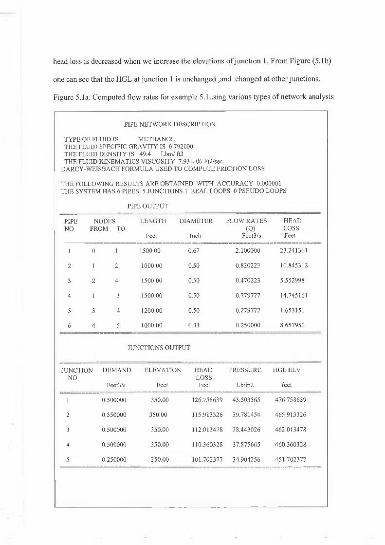
head loss is decreased when we increase the elevations of junction 1. From Figure (5.1h)

one can see that the HGL at junction 1 is unchanged ,and changed at other junctions.

Figure 5.1a. Computed flow rates for example 5.1using various types of network analysis

PIPE NETWORK DESCRIPTION

TYPE OF FLUID IS METHANOL THE FLUID SPECIFIC GRAVITY IS 0.792000 THE FLUID DENSITY IS 49.4 Lbm/ ft3 THE FLUID KINEMATICS VISCOSITY 7.93E-06 Ft2/sec

DARCY-WEISBACH FORMULA USED TO COMPUTE FRICTION LOSS

THE FOLLOWING RESULTS ARE OBTAINED WITH ACCURACY 0.000001 THE SYSTEM HAS 6 PIPES 5 JUNCTIONS 1 REAL LOOPS 0 PSEUDO LOOPS

PIPE OUTPUT

PIPENO

NODES FROM TO

LENGTH DIAMETER

Feet Inch

FLOW RATES(Q)

Feet3/s

HEADLOSSFeet

1 0 1 1500.00 0.67 2.100000 23.241361

2 1 2 1000.00 0.50 0.820223 10.845312

3 2 4 1500.00 0.50 0.470223 5.552998

4 1 3 1500.00 0.50 0.779777 14.745161

5 3 4 1200.00 0.50 0.279777 1.653151

6 4 5 1000.00 0.33 0.250000 8.657950

JUNCTIONS OUTPUT

JUNCTION DEMAND NO

ELEVATION HEADLOSS

PRESSURE HGL ELV

Feet3/s Feet Feet Lb/in2 feet

1 0.500000 350.00 126.758639 43.503565 476.758639

2 0.350000 350.00 115.913326 39.781454 465.913326

3 0.500000 350.00 112.013478 38.443026 462.013478

4 0.500000 350.00 110.360328 37.875665 460.360328

5 0.250000 350.00 101.702377 34.904256 451.702377

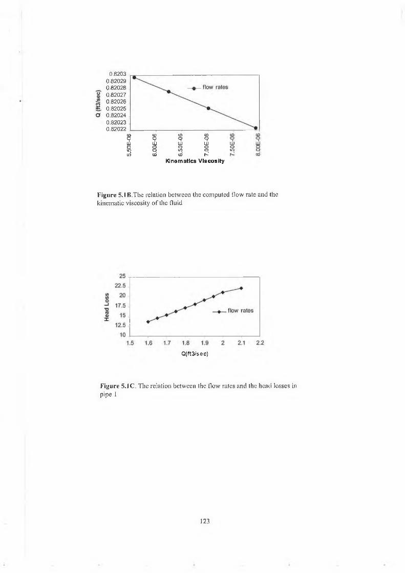
0.82030.820290.820280.820270.820260.820250.820240.820230.82022

CD CO CD CDO 9 9 9LU LLi HI HIo o oid O in ou5 CD CD h»'

LUOin oo

Kinematics V iscosity

Figure S.IB.The relation between the computed How rate and the kinematic viscosity of the fluid

Q(ft3/sec)

Figure 5.1C. The relation between the flow rates and the head losses in pipe 1

123

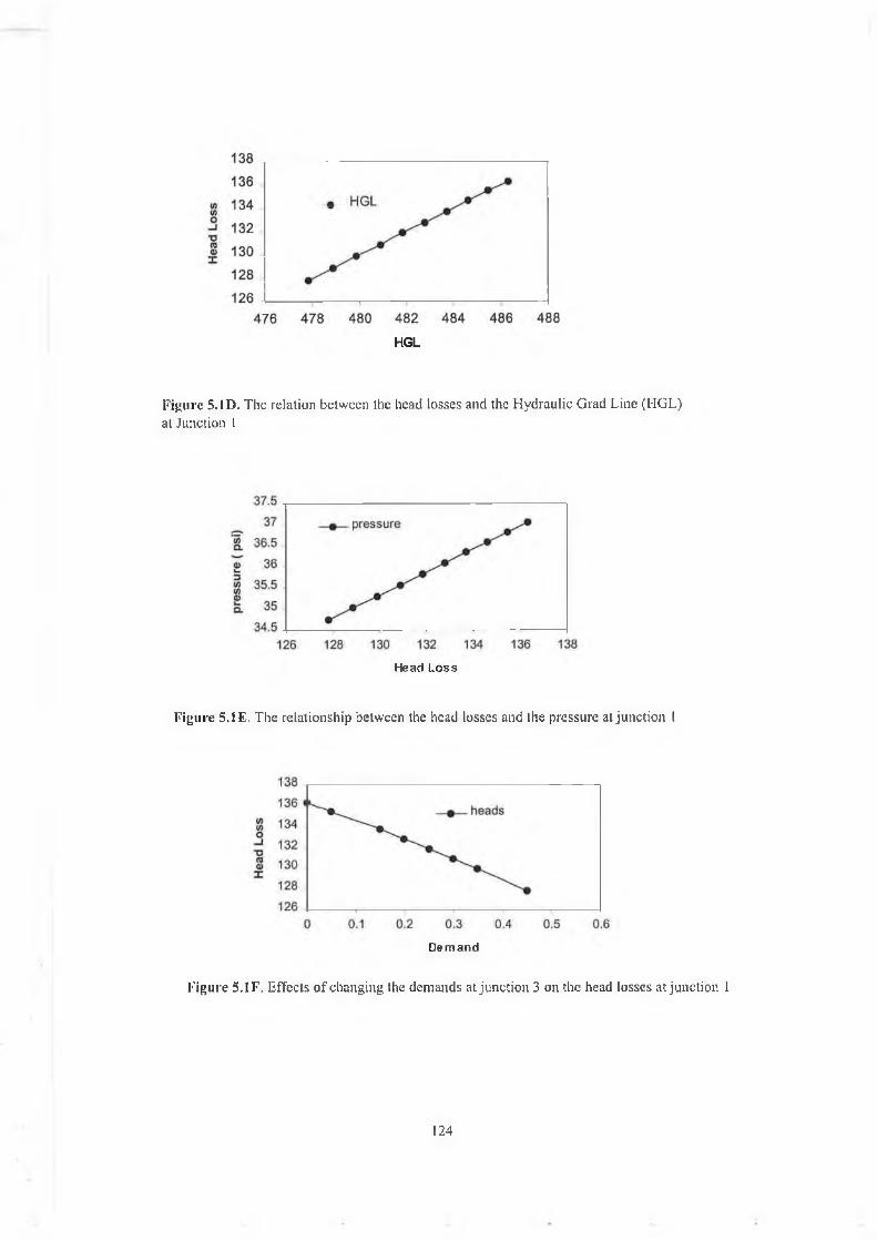
H G L

Figure 5 .ID. The relation between the head losses and the Hydraulic Grad Line (HGL) at Junction 1

Head Loss

Figure 5.1 E. The relationship between the head losses and the pressure at junction 1

Demand

Figure 5. IF. Effects o f changing the demands at junction 3 on the head losses at junction 1

124

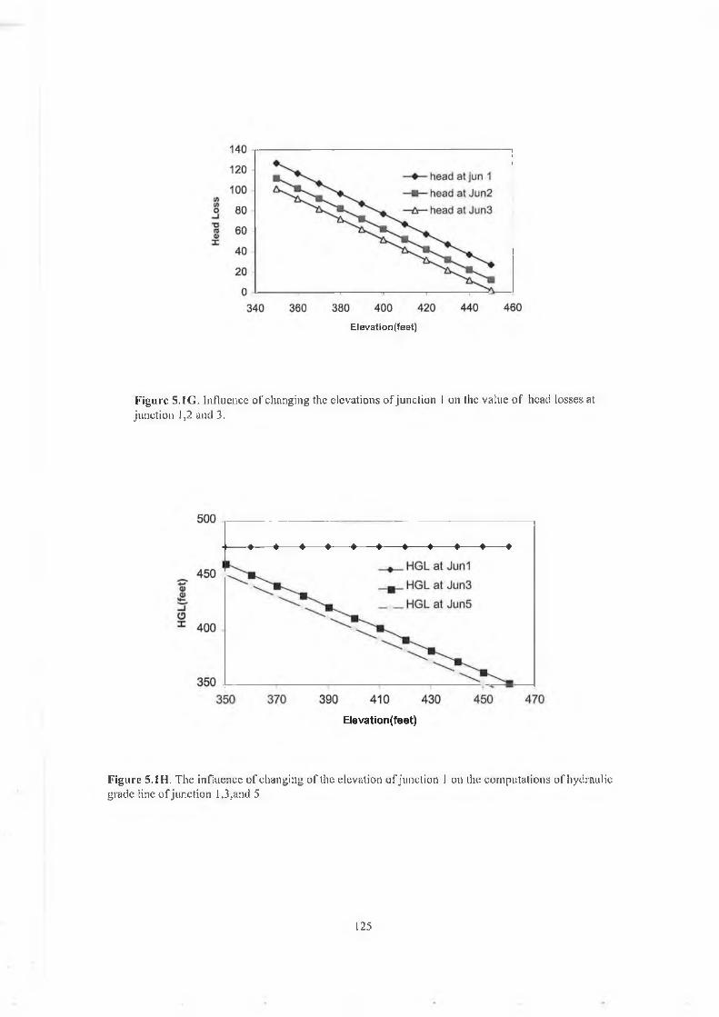
Elevation(feet)

Figure 5.1G. Influence o f changing the elevations o f junction 1 on the value o f head losses at junction 1,2 and 3.

Elevation(feet)

Figure 5.1H. The influence o f changing o f the elevation ofjunction 1 on the computations ofhydraulic grade line ofjunction 1,3,and 5

125

This example concentrates on the implementation of solution to networks using the

computer program, and how pumps are readily included. To begin this process consider

first the seven-pipe network in Figure (5.2) that includes a source pump that supplies

some of the system demand.

For this network there are four junction continuity equations and three loop energy

equations. The Q-equations are

Junction continuity equations

Example 5 .2 .

There is one real loop in the network, so the energy equation around the real loop is

Two pseudo loops are required. A possibility is one pseudo loop connecting the

reservoirs supplying pipes 1 and 5 through pipes 1,6,4,and 5; and the other connects the

pump reservoir and the reservoir supplying pipe 1 through pipes 1,6,7.

The energy equations around these two loops are

At junction [ 1 ] - Q\ + Qi + Qe ~ 0

At junction [ 2 ] - Q 2- Q 3 = -2.0

At junction [ 3 ] Q3 - Q 4 - Q s = 0

At junction [ 4 ] 0 4 - 0 6 - 2 7 = 0

K2Q2"‘ - K-,03* - K g ? - K 6Q6- = 0.0

K g ? + K 6Q ? - K & ' - h pump = 100-95

126

in solving the system of equations, the introduction of the transformation described in

chapter 3. There will be an extra additional unknown, i.e. the pump head is written in

the form of a quadratic equation as follow

hP = -10.330;; + 2.8230,, + 22.29

This transformation replaced hp by

hp = -10.33 G2 + 2.823G + 22.29

And adding the following linear equation to the system:

~ 0 7 + G = = -0.1377 2 A

in which G is the new transformation variable.

Should any flow rate Q becomes negative during the solution process, the computed

direction of flow is in the opposite direction that assumed in writing the equations.

The output of the program is show in Figure (5.2a)

Several observations can be concluded from the output result. First the same behavior

was noted regarded the relation between the flow rate and head losses as discussed in the

previous example. Different changes are now made on the components of the pipe

network. If one starts with the change the length of pipe 1 to see how it affects the results,

from Figure (5.2b) we can notice that the flow rates in pipe 1 is decreased when the

length is increased, it is the same for the relation between the head losses and the flow

rates in pipe 1 . The same has been noted with the change of the diameter in pipe 1 , this

shown in Figure (5.2 c,5.2d).

Form these two figures , the flow rate is increases when the diameter of the pipe is

larger, and consequently the head losses are decrease when the diameter is getting

smaller as shown in Figure (5.2e).

127

If the length o f pipe 7 is changed, which contains the pump, one can see that the flow

rate has the same behavior as in Figure (5.2b, 5.2c), this is shown in Figure (5.2f, 5.2g).

For the head produced by the pump, the change in the length o f the pipe shows that the

head produced by pump is increased with the increase in length o f the pipe containing the

pump, as shown in Figure (5.2h, 5.2i).

If a change in the diameter is applied in pipe 7 it will be seen that the head produced by

the pump is decreased when the diameter is bigger, this is applied for the head losses in

that pipe as shown in Figure (5.2j).

128

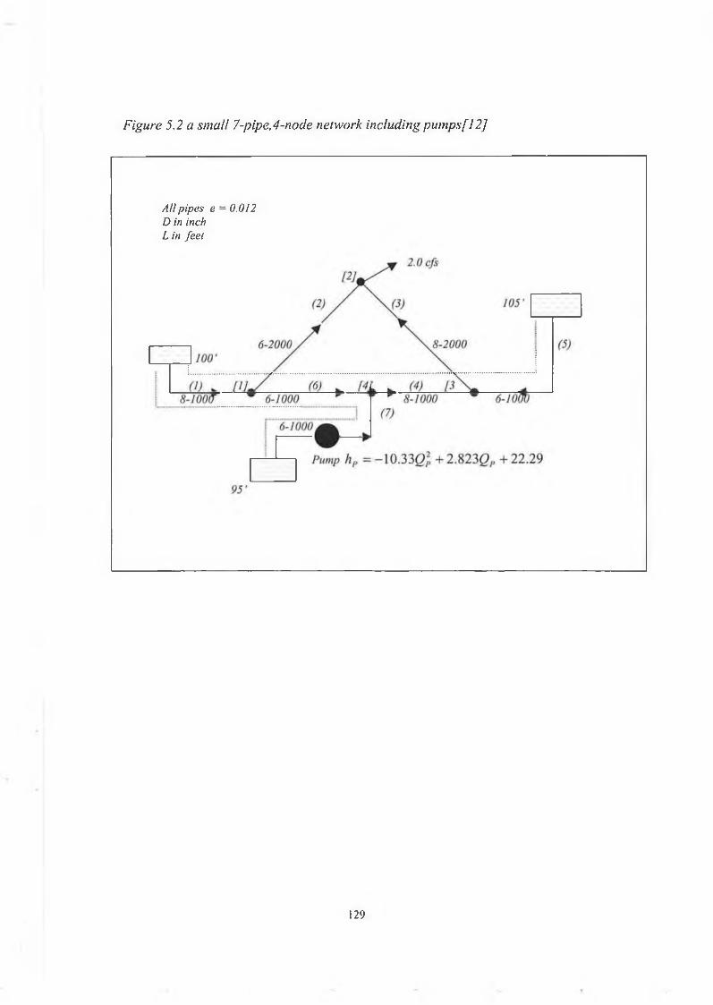
Figure 5.2 a small 7-pipe,4-node network includingpumps[12]

All pipes e = 0.012 D in inch L in feet

129

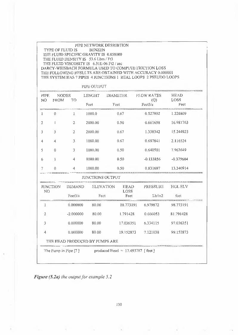
PIPE NETWORK DESRIBTION TYPE OF FLUID IS BENZEN

THE FLUID SPECIFIC GRAVITY IS 0.858000 THE FLUID DENSITY IS 53.6 Lbm / Ft3 THE FLUID VISCOSITY IS 6.3 IE-06 Ft2 / sec

DARCY-WEISBACH FORMULA USED TO COMPUTE FRICTION LOSS THE FOLLOWING RESULTS ARE OBTAINED WITH ACCURACY 0.000001 THE SYSTEM HAS 7 PIPES 4 JUNCTIONS 1 REAL LOOPS 2 PSEUDO LOOPS

PIPE OUTPUT

PIPENO

NODES LENGHT FROM TO

Feet

DIAMETER FLOW RATES(Q )

Feet Feet3/s

HEADLOSS

Feet

1 0 1 1000.0 0.67 0.527802 1.226809

2 1 2 2000.00 0.50 0.661658 16.981763

3 3 2 2000.00 0.67 1.338342 15.244923

4 4 3 1000.00 0.67 0.697841 2.116524

5 0 3 1000.00 0.50 0.640501 7.963649

6 1 4 1000.00 0.50 -0.133856 -0.379684

7 0 4 1000.00 0.50 0.831697 13.340914

JUNCTIONS OUTPUT

JUNCTIONNO

DEMAND

Feet3/s

ELEVATION HEAD LOSS

Feet Feet

PRESSURE

Lb/in2

HGLELV

feet

1 0 . 0 0 0 0 0 0 80.00 18.773191 6.979872 98.773191

2 -2.000000 80.00 1.791428 0.666053 81.791428

3 0.000000 80.00 17.036351 6.334115 97.036351

4 0.000000 80.00 19.152873 7.121038 99.152873

THE HEAD PRODUCED BY PUMPS ARE

The Pump in Pipe [7 ] produced Head = 17.493787 [feet]

Figure (5.2a) the output for example 5.2

130

L(feet)

Figure 5.2B. Effects o f changing the length of pipe 1 on the computations of the flow rales in pipe 1

Q(ft3/sec)

Figure 5.2C. The established relation between the flow rates and the head losses in pipe 1 at different lengths

131

D(lnch)

Figure 5.2D. liffccts o f diameter changing on the computed flow rates in pipe I

D(inch)

Figure 5.2E. Effects o f changing the diameter o f pipe I on the head losses in pipe 1 computations

132

L (fee t)

Figure 5.2F. Effects o f lengths changes in the pipe containing the pump oil the flow rates through the pipe

L(feet)

Figure 5.2G. Effects o f lengths changes in the pipe containing the pump on head losses computation in that pipe

133

L (feet)

Figure 5.2H. Effects o f the length changes in the pipe containing the pump on the head produced by the pump

Q (ft3 /sec)

Figure 5.2 I. The established relationship between the flow rate in the pipe containing the pump the head produced by the pump in that pipe

134

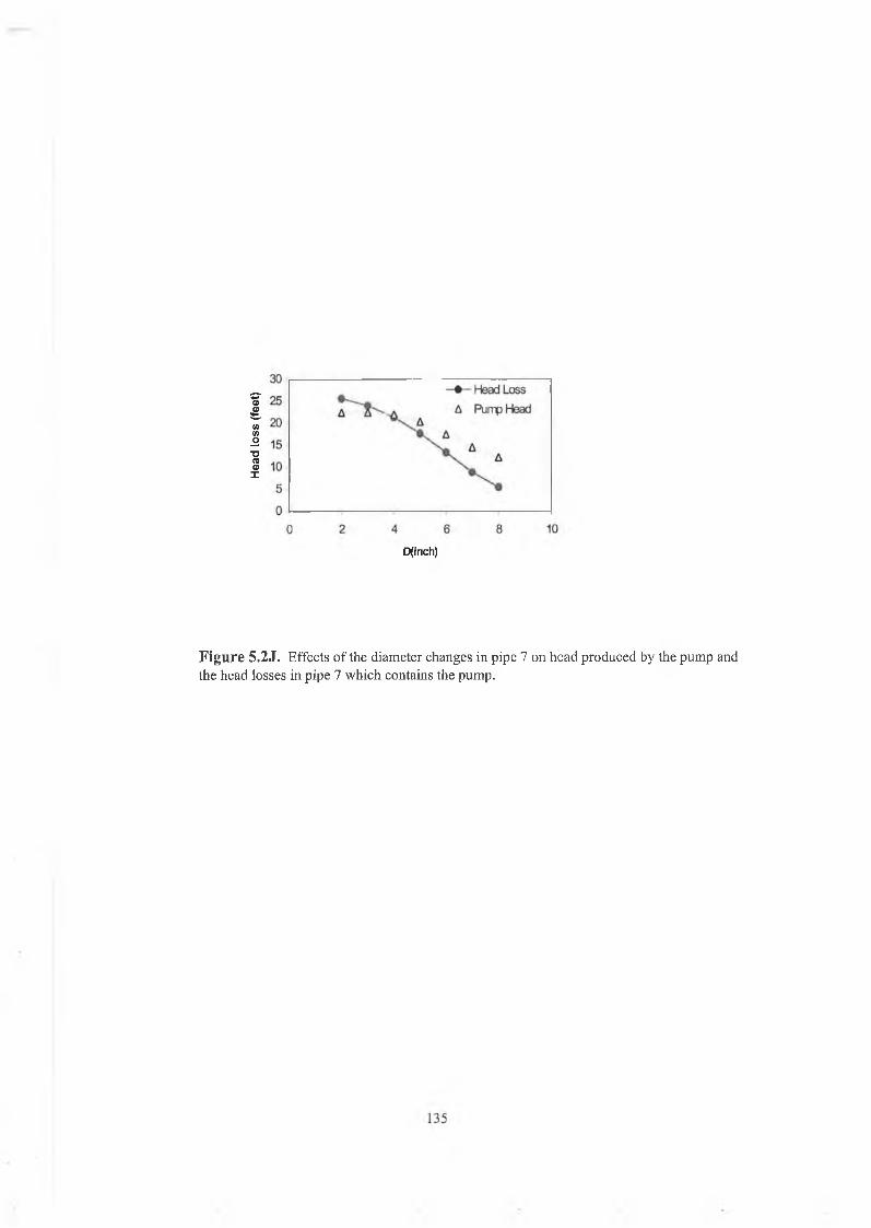
Head

lo

ss

(fee

t)

D(inch)

Figure 5.2J. Effects of the diameter changes in pipe 7 on head produced by the pump andthe head losses in pipe 7 which contains the pump.

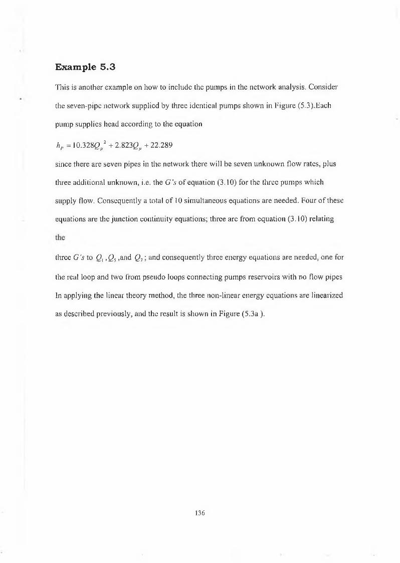
This is another example on how to include the pumps in the network analysis. Consider

the seven-pipe network supplied by three identical pumps shown in Figure (5.3).Each

pump supplies head according to the equation

hP = 10 .3280/ + 2.8230,, + 22.289

since there are seven pipes in the network there will be seven unknown flow rates, plus

three additional unknown, i.e. the G's of equation (3.10) for the three pumps which

supply flow. Consequently a total of 10 simultaneous equations are needed. Four of these

equations are the junction continuity equations; three are from equation (3.10) relating

three G's to O, , 0 5 ,and 0 7; and consequently three energy equations are needed, one for

the real loop and two from pseudo loops connecting pumps reservoirs with no flow pipes

In applying the linear theory method, the three non-linear energy equations are linearized

as described previously, and the result is shown in Figure (5.3a ).

Exam ple 5 .3

136

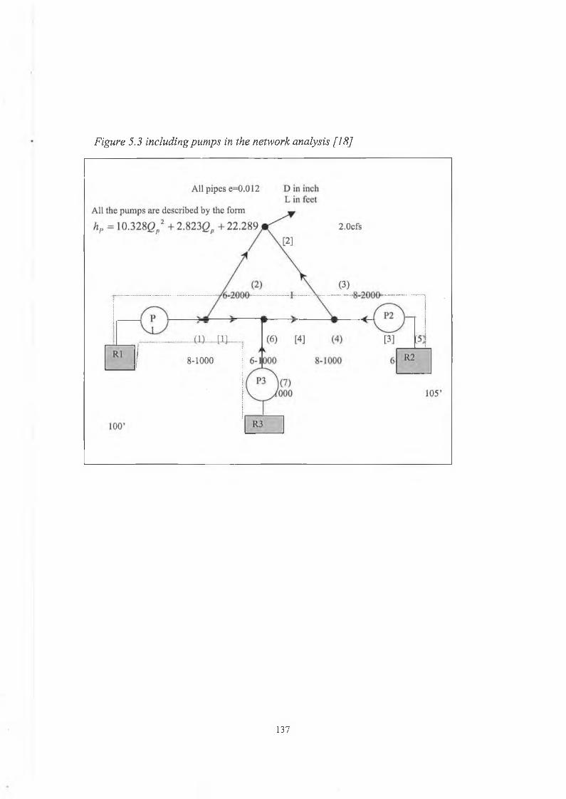
Figure 5.3 including pumps in the network analysis [18]

137

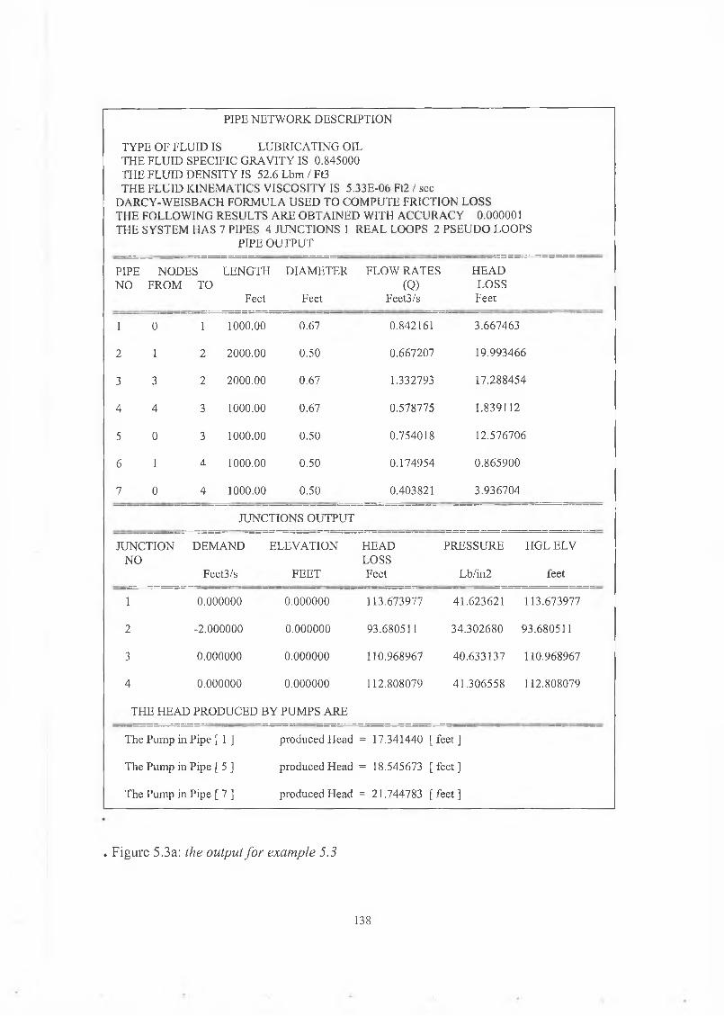
TYPE OF FLUID IS LUBRICATING OIL THE FLUID SPECIFIC GRAVITY IS 0.845000 THE FLUID DENSITY IS 52.6 Lbm / Ft3 THE FLUID KINEMATICS VISCOSITY IS 5.33E-06 Ft2 / sec

DARCY-WEISBACH FORMULA USED TO COMPUTE FRICTION LOSS THE FOLLOWING RESULTS ARE OBTAINED WITH ACCURACY 0.000001 THE SYSTEM HAS 7 PIPES 4 JUNCTIONS 1 REAL LOOPS 2 PSEUDO LOOPS

PIPE OUTPUT

PIPE NETWORK DESCRIPTION

PIPENO

NODES LENGTH FROM TO

Feet

DIAMETER

Feet

FLOW RATES HEAD (Q) LOSS

Feet3/s Feet

1 0 1 1000.00 0.67 0.842161 3.667463

2 1 2 2000.00 0.50 0.667207 19.993466

3 3 2 2000.00 0.67 1.332793 17.288454

4 4 3 1000.00 0.67 0.578775 1.839112

5 0 3 1000.00 0.50 0.754018 12.576706

6 1 4 1000.00 0.50 0.174954 0.865900

7 0 4 1000.00 0.50 0.403821 3.936704

JUNCTIONS OUTPUT

JUNCTION DEMAND ELEVATION HEAD PRESSURE HGL ELVNO LOSS

Feet3/s FEET Feet Lb/in2 feet

1 0.000000 0.000000 113.673977 41.623621 113.673977

2 -2.000000 0.000000 93.680511 34.302680 93.680511

3 0.000000 0.000000 110.968967 40.633137 110.968967

4 0.000000 0.000000 112.808079 41.306558 112.808079

THE HEAD PRODUCED BY PUMPS ARE

The Pump in Pipe [ 1 ] produced Head = 17.341440 [feet]

The Pump in Pipe [ 5 ] produced Head = 18.545673 [feet]

The Pump in Pipe [ 7 ] produced Head = 21.744783 [feet]

. Figure 5.3a: the output for example 5.3

138

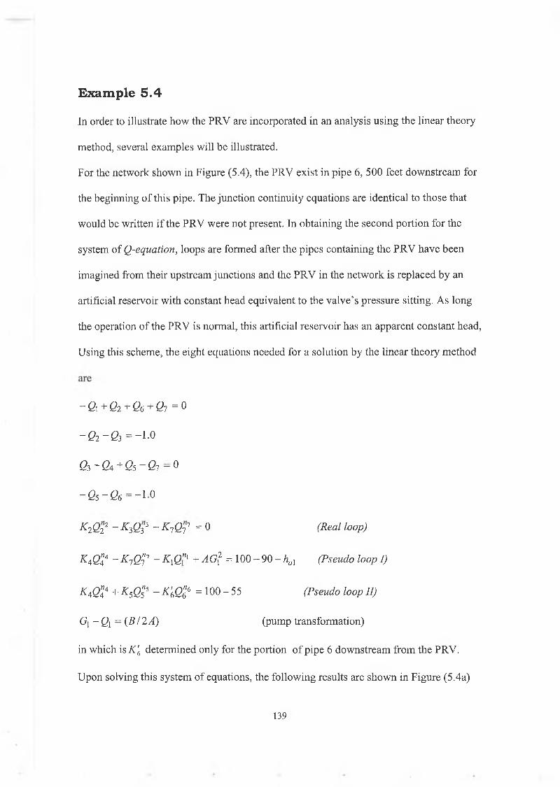
In order to illustrate how the PRV are incorporated in an analysis using the linear theory

method, several examples will be illustrated.

For the network shown in Figure (5.4), the PRV exist in pipe 6 , 500 feet downstream for

the beginning o f this pipe. The junction continuity equations are identical to those that

would be written if the PRV were not present. In obtaining the second portion for the

system o f Q-equation, loops are formed after the pipes containing the PRV have been

imagined from their upstream junctions and the PRV in the network is replaced by an

artificial reservoir with constant head equivalent to the valve’s pressure sitting. As long

the operation o f the PRV is normal, this artificial reservoir has an apparent constant head,

Using this scheme, the eight equations needed for a solution by the linear theory method

- Q\ + Qi + 06 + Qi = o

- 0 2 -0 3 = " 1 .0

Qs ~ Qa + Q5 ~ Qi - 0

- 0 5 - 0 6 = - 1 0

K 2 Q2 2 ~ K3Qy3 - KiQi 1 = 0 (Real 1o°p)

K4 Q^ - KnQ^ - K{Q" 1 + AG? = 100 - 90 - hol (Pseudo loop I)

K4 QZ4 + ^ 5 0 5" 5 - K'6Qle = 1 0 0 - 5 5 (Pseudo loop II)

Gi~Qi= (B HA) (pump transformation)

in which is K[ determined only for the portion o f pipe 6 downstream from the PRV.

Upon solving this system o f equations, the follow ing results are shown in Figure (5.4a)

Exam ple 5 .4

139

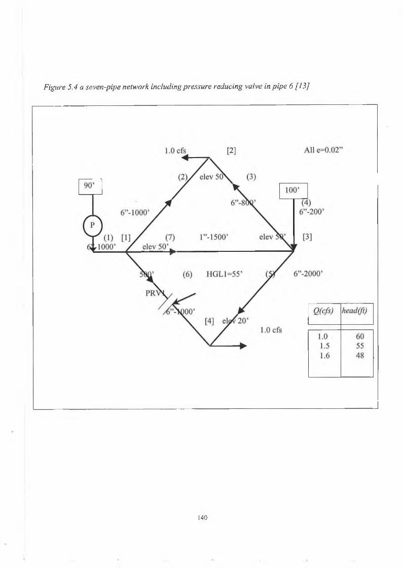
Figure 5.4 a seven-pipe network including pressure reducing valve in pipe 6(13]

140

From the output o f this example which is shown in Figure (5.4a) w e could notice that the

pressure upstream from the PRV equals the 121.97ft. and the downstream equals 54.98 ft.

consequently , the assumption used in writing the final loop equation is correct.

Changing the assumption and setting the pressure downstream equal to 40 ft, figure

(5.4a2), shows that the flow rates in pipe 6 which contains the pressure reducing valves is

a negative flow rate. This assumption is incorrect, since the PRV would then have acted

as check valve and allowed the elevation o f the HGL downstream from the PRV to rise

above 40 ft. the flow rate in pipe 6 would no longer be unknown, but equal to zero. And

this causes the PRV to shut off. The computer program is capable o f warning the user if

the PRV is operating normally or not.

Another assumptions has been applied to this network by setting the HGL at various

values and Figure (5.4b) shows the effect o f setting the elevation o f the artificial

reservoir.

Several other observations can be established by changing the geometry o f the network.

Making a change to the location o f the PRV , for example 400 feet down stream for the

beginning o f pipe 6 , one shall notice that locations o f the PRV have slight effect on the

calculation o f the flow rates through the pipe; Figure (5.4c) and (5.4d) shown that.

In figures (5.4e),(5.4f) and (5.4g) the same behavior o f changing the diameter in the

pipe containing the PRV was noted as discussed in example 5.2

Another important observation has been noted when applying the change o f the demand

on junctions, first the change is applied in junction 2. One can see that the flow rate in the

pipe 6 is always positive with certain amount to be drawn from the system. If the amount

on the demand is decreased to less than 0.5 cfs as shown in Figure (5.4h), the flow rate in

141

pipe 6 w ill be negative , which means that the PRV w ill act as Check valve and cause the

valve to shut o ff as discussed earlier.

If the demand is changed at junction 4 one w ill get similar behavior, this shown in

Figure (5.4k).

142

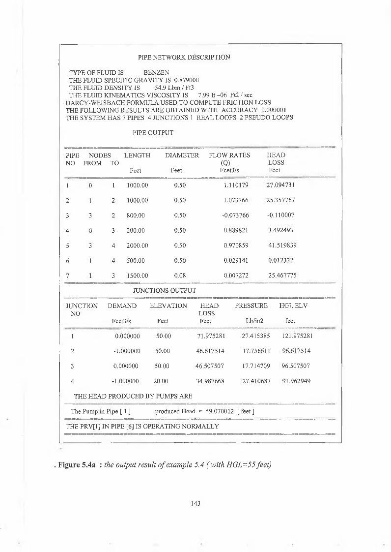
TYPE OF FLUID IS BENZEN THE FLUID SPECIFIC GRAVITY IS 0.879000 THE FLUID DENSITY IS 54.9 Lbm / Ft3 THE FLUID KINEMATICS VISCOSITY IS 7.99 E -06 Ft2 / sec

DARCY-WEISBACH FORMULA USED TO COMPUTE FRICTION LOSS THE FOLLOWING RESULTS ARE OBTAINED WITH ACCURACY 0.000001 THE SYSTEM HAS 7 PIPES 4 JUNCTIONS 1 REAL LOOPS 2 PSEUDO LOOPS

PIPE OUTPUT

PIPE NETWORK DESCRIPTION

PIPENO

NODES FROM TO

LENGTH

Feet

DIAMETER

Feet

FLOW RATES(Q )Feet3/s

HEADLOSSFeet

1 0 1 1000.00 0.50 1.110179 27.094731

2 1 2 1000.00 0.50 1.073766 25.357767

3 3 2 800.00 0.50 -0.073766 -0.110007

4 0 3 200.00 0.50 0.889821 3.492493

5 3 4 2000.00 0.50 0.970859 41.519839

6 1 4 500.00 0.50 0.029141 0.012332

7 1 3 1500.00 0.08 0.007272 25.467775

JUNCTIONS OUTPUT

JUNCTIONNO

DEMAND

Feet3/s

ELEVATION

Feet

HEADLOSSFeet

PRESSURE

Lb/in2

HGL ELV

feet

1 0.000000 50.00 71.975281 27.415385 121.975281

2 -1.000000 50.00 46.617514 17.756611 96.617514

3 0.000000 50.00 46.507507 17.714709 96.507507

4 -1.000000 20.00 34.987668 27.410687 91.962949

THE HEAD PRODUCED BY PUMPS ARE

The Pump in Pipe [ 1 ] produced Head = 59.070012 [ feet j

THE PRV[1] IN PIPE [6] IS OPERATING NORMALLY

. Figure 5.4a : the output result of example 5.4 ( with HGL=55 feet)

143

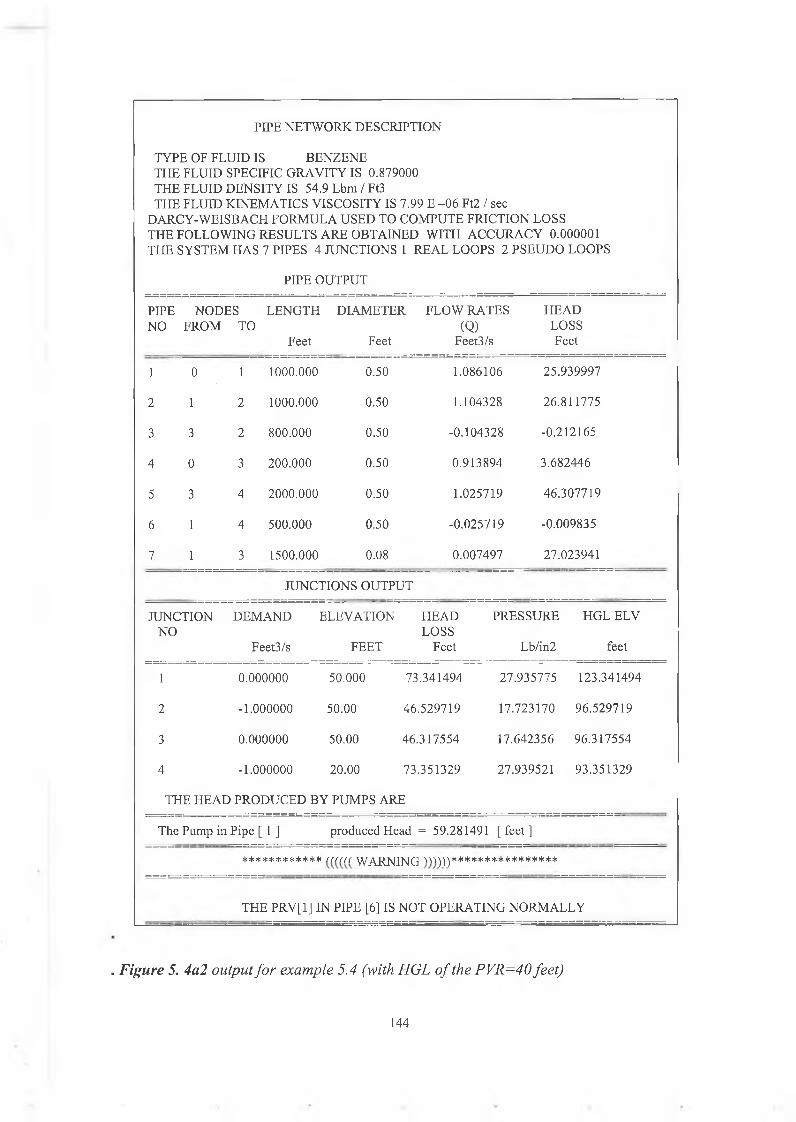
TYPE OF FLUID IS BENZENE THE FLUID SPECIFIC GRAVITY IS 0.879000 THE FLUID DENSITY IS 54.9 Lbm / Ft3 THE FLUID KINEMATICS VISCOSITY IS 7.99 E -06 Ft2 / sec

DARCY-WEISBACH FORMULA USED TO COMPUTE FRICTION LOSS THE FOLLOWING RESULTS ARE OBTAINED WITH ACCURACY 0.000001 THE SYSTEM HAS 7 PIPES 4 JUNCTIONS 1 REAL LOOPS 2 PSEUDO LOOPS

PIPE OUTPUT

PIPE NETWORK DESCRIPTION

PIPE NODES LENGTH DIAMETER FLOW RATES HEADNO FROM TO (Q) LOSS

Feet Feet Feet3/s Feet

1 0 1 1000.000 0.50 1.086106 25.939997

2 1 2 1000.000 0.50 1.104328 26.811775

3 3 2 800.000 0.50 -0.104328 -0.212165

4 0 3 200.000 0.50 0.913894 3.682446

5 3 4 2000.000 0.50 1.025719 46.307719

6 1 4 500.000 0.50 -0.025719 -0.009835

7 1 3 1500.000 0.08 0.007497 27.023941

JUNCTIONS OUTPUT

JUNCTIONNO

DEMAND

Feet3/s

ELEVATION

FEET

HEAD PRESSURE HGL ELV LOSS

Feet Lb/in2 feet

1 0.000000 50.000 73.341494 27.935775 123.341494

2 -1.000000 50.00 46.529719 17.723170 96.529719

3 0.000000 50.00 46.317554 17.642356 96.317554

4 -1.000000 20.00 73.351329 27.939521 93.351329

THE HEAD PRODUCED BY PUMPS ARE

The Pump in Pipe [ 1 ] produced Head = 59.281491 [ feet ]

************ ru in WARNING ' A Y ) ' ) ' ) * * * * * * * * * * * * * * * *

THE PRV[1] IN PIPE [6] IS NOT OPERATING NORMALLY

. Figure 5. 4a2 output for example 5.4 (with HGL of the PVR-40 feet)

144

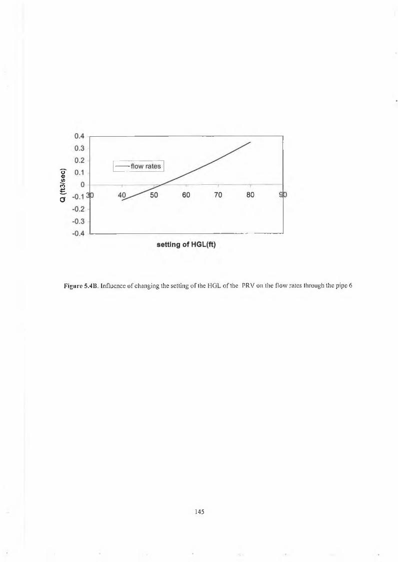
Q (ft

3/se

c)

Figure 5.4B. Influence of changing the setting of the I1GL of the PRV on the flow rates through the pipe 6

145

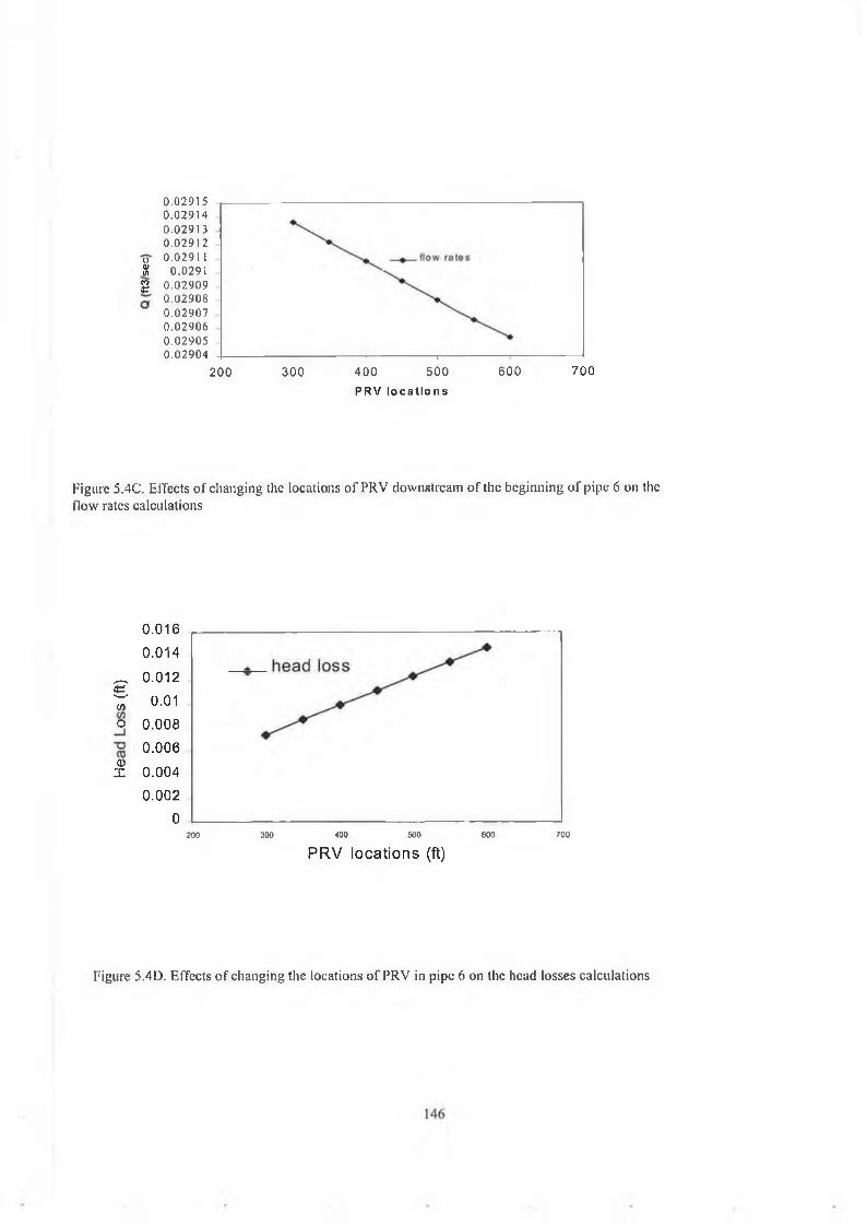
0.029150.029140.029130.02912

t ) 0.0291 141in 0.0291

COr 0.02909

0.029080.029070.029060.029050.02904

200 3 00 400 500 600 700

P R V lo c a t io n s

Figure 5.4C. Effects of changing ihc locations of PRV downstream of the beginning of pipe 6 on the flow rates calculations

0.0160.014

_ 0.012

I 0.01o 0.008

0.0060)X 0.004

0.002 0

200 300 400 600 600 700

PRV locations (ft)

—-------- r

Figure 5.4D. Effects of changing the locations of PRV in pipe 6 on the head losses calculations

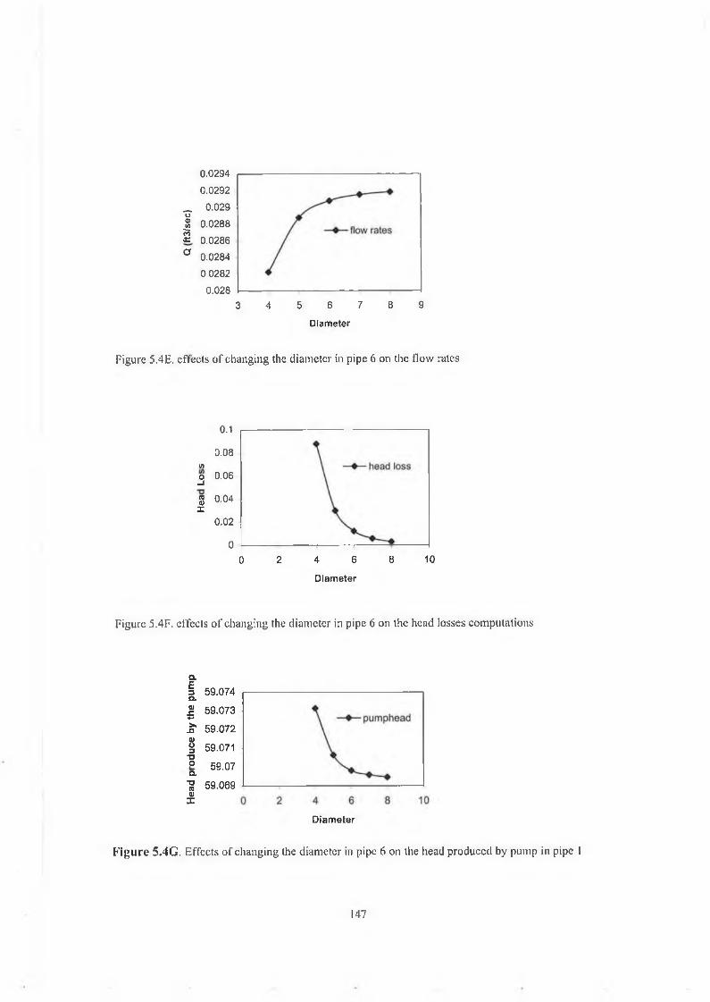
0.0294

0.0292

_ 0.029

| 0.0288

S 0.0286

° 0,0284

0,0282

0.0283 4 5 6 7 8 9

Diameter

Figure 5.4E. cffccts of changing the diameter in pipe 6 on the flow rates

0.1

0.08v>o 0.06_j8 0.04 x

0.02

00 2 4 6 8 10

Diameter

Figure 5.4F. cffccts of changing the diameter in pipe 6 on the head losses computations

aE3 59.074a.a>£ 59.073*-*>».a 59.072

83 59.071■uo 59.07a

T3ra 59.0690>X

Diameter

Figure 5.4G, Effects of changing the diameter in pipe 6 on the head produced by pump in pipe l

147

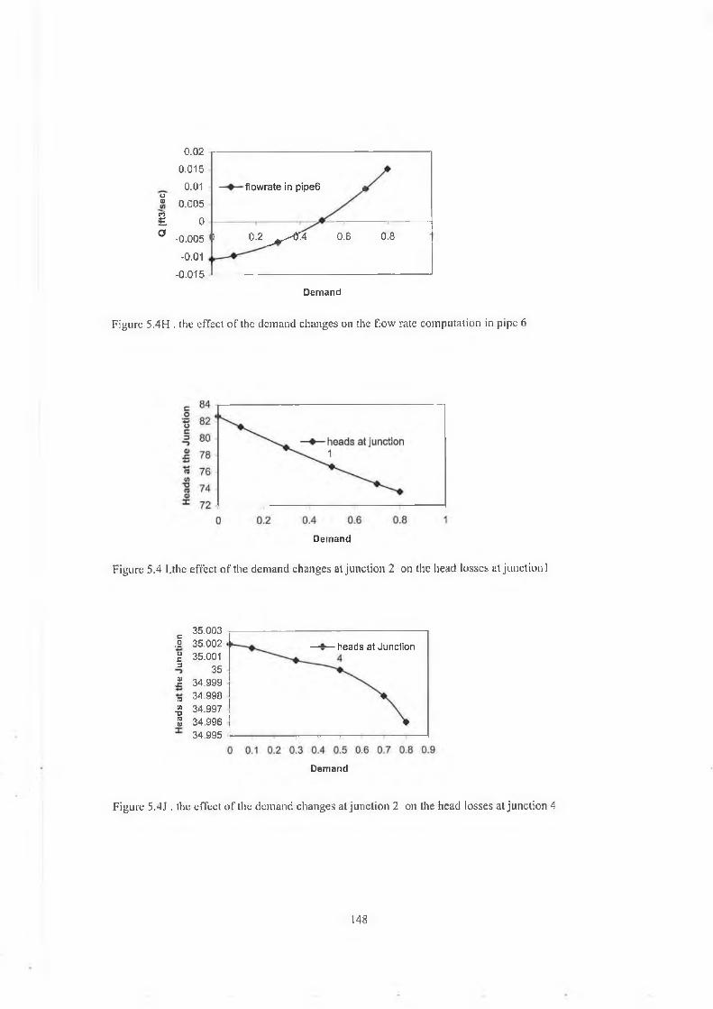
0.02

0.015

0.01uID 0.005ri£ 0o

-0.005

-0.01

-0.015

— flowrate in pipe6 4

) 0.2 ^ * ^ 4 0.6 0.8

Demand

Figure 5.4H . the cffcct of the demand changes on the flow rate compulation in pipe 6

Demand

Figure 5.4 I.the cffcct of the demand changes at junction 2 on the head losses at junction 1

C.2oc3Q>JCGJWTJro<u

35.00335.00235.001

3534.99934.99834.99734.99634.995

heads at Junction

Demand

Figure 5.4J . the effect of the demand changes at junction 2 on the head losses at junction 4

148

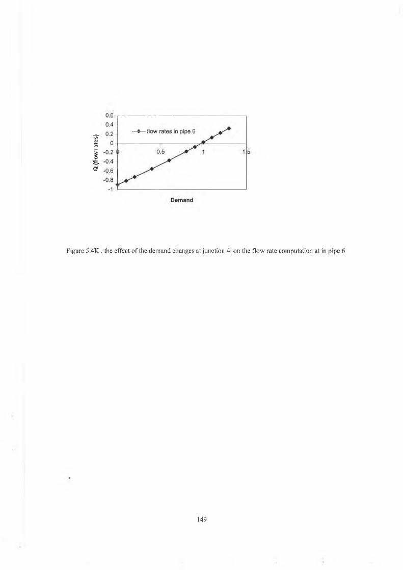
Q (flo

w ra

tes)

Figure 5.4K . the effect of the demand changes at junction 4 on the flow rate computation at in pipe 6

149

CHAPTER 6

Conclusion and Suggestion For Further Work

6.1 Conclusion

The present project deals with the steady flow analysis o f incompressible, single­

phase fluid flow s and the computer program developed is general purpose in nature.

A number o f case studies have been carried out using the program.

Based on verification made using these case studies the fo llow ing conclusion can be

drawn.

The linear theory method o f analysis o f networks o f pipes and pumps provides a

convenient method for a simulation. In particular it enables the network to be

specified in very simple terms.

The simulation calculates the flow rate in each pipe, the head loss in each pipe can be

easily calculated, and the head loss and the pressure at each junction.

The simulation makes use o f several numerical methods to sim plify the computation

such as Gauss elimination method to solve linear simultaneous equations. These

computer programs are discussed in appendix (A) and can be summarised as follow

1) A computer program is written to calculate the friction head loss / when the

Darcy-W eisbach is implemented to compute the head friction.

2) Polynom ial least square method is implemented to represent the head produced

by pumps in the computation when the pumps are described by operation data.

The computer program is capable o f fitting the pump’s operating data from the

150

pump characteristic curve by approximating the head produced by pumps over its

working range by a quadratic second order equation.

3) Gauss elimination with partial pivoting method has been used to solve the set o f

linear simultaneous equation since it is one o f the m ost w idely direct methods

However, the program has certain limitations.

• It can not take into account pumps described by horse power

• In the case o f including the pressure reducing valve in the pipe networks, the

program can indicate if the valves are operating normally or not, but can not

rewrite the model o f equations to give the precise solutions for the setting o f the

hydraulic grade line o f the PRV.

6.2 Suggestion for further work

Further work could be carried out to link this present study to a real more

comprehensive computer simulation o f pipe flow network in a refinery complex.

Some suggestions for further work are listed as follows:

i. This computer program can be developed to accommodate the non-Newtonian

liquid or mixtures including correction for changes in properties with

temperature and pressure

ii. Incorporate the linear theory method to simulate the two-phase flow pipeline

networks

iii. The effect o f heat loss on pressure drop can be predicted by developing the

model to calculate the fluid temperature profile based on the operation

condition.

iv. In addition, studies dealing with unsteady flows or transient problems,

operation and control, acquisition o f supply, optimisation o f network

performance against cost, should be given consideration.

151

R eferen ces

R eferen ces:

1- Rojiani, K am al B., ” p r o g r a m m in g i n C w it h N u m e r i c a l m e t h o d s f o r

E n g i n e e r s , ” P r e n t i c e - H a l l , In c , N e u > J e r s e y , 1 s t e d it io n , 1 9 9 6 .

2- Holmes, B arry.,” Through C to C ++” Jones and B a r tle tt

p u b l i s h e r s , S u d b u r y , M A , 1 st e d it io n s , 1 9 9 7 .

3- William, H. P, e t a l.,” N u m e r i c a l R e c i p e s i n C ” C a m b r i d g e U n i v e r s i t y

P r e s s , C a m b r i d g e , 1 st e d it io n 1 9 8 8 .

4- Herbert, S ch ild t.,” C : T h e C o m p le t e R e f e r e n c e , " M e G r a w H i l l , 1 st

e d it io n , 1 9 8 7 .

5- Wood, D. J. & Charles, C.O.A.,” H y d r a u l i c N e t w o r k A n a l y s i s U s i n g

L i n e a r T h e o r y , ” J o u r n a l o f t h e H y d r a u l i c s J o u r n a l o f t h e H y d r a u l i c s

D i v i s i o n , A S C E , V o l.9 8 , P r o c . P a p e r 9 0 3 1 , J u l y 1 9 7 2 , p p 1 1 5 7 - 1 1 7 0 .

6- Martin, D.W.& Peters, G., ”t h e a p p l i c a t i o n o f N e w t o n ’s m e t h o d to

n e t w o r k a n a l y s i s b y d i g i t a l c o m p u t e r , ” J o u r n a l o f t h e I n s t it u t e o f W a t e r

E n g i n e e r s , V o l. 1 7 , 1 9 6 3 , p p . 1 1 5 - 1 2 9 .

7- Cross, H., ”a n a l y s i s o f f l o w i n n e t w o r k s o f c o n d u it s o r c o n d u c t o r s , ”

1 9 3 6 . U n i v e r s i t y o f I l l i n o i s B u l l 2 8 6 .

8- Holland, F.A. & Bragg, R .,” F l u i d F l o w f o r C h e m i c a l E n g i n e e r s , ”

E d w a r d A r n o l d , 2 nd e d it io n , 1 9 9 5 .

153

9- Irving H. S ham es./1 M e c h a n i c s o f F l u i d s / ’ M c G r a w - H i l l , 3 rd e d it io n ,,

1 9 9 2 .

10- Cheremisinoff, Nicolas P .,” F l u i d F l o w : P u m p s , P i p e s a n d

C h a n n e l s , ” A n n A r b o r S c ie n c e , A n n A r b o r , M i c h i g a n , 2 nd e d it io n , 1 9 8 2 .

11- Tullis, J.Paul.” H y d r a u l i c s o f P i p e l i n e s : P u m p s , V a lv e s , C a v it a t io n ,

T r a n s i e n t s , ” J o h n W ile y & s o n s , I n c , 1 s t e d it io n , 1 9 8 9 .

12- Jepson, R., ” a n a l y s i s o f f l o w i n p i p e n e t w o r k s , ” A n n A r b o r S c ie n c e ,

A n n A r b o r , M ic h ig a n , 1 9 7 6 .

13- Bruce E. Larock, Roland W. Jeppson, & Gary Z. W atters.”

H y d r a u l i c s o f P i p e l i n e S y s t e m s , ” C R C P r e s s L L C , 1 st e d it io n , 1 9 9 9 .

14- Colebrook, C. F., ” T u r b u le n t f l o w in p i p e s , w it h p a r t i c u l a r

r e f e r e n c e to t h e t r a n s i t io n r e g io n b e t w e e n t h e s m o o t h a n d r o u g h p i p s

l a w s , ” J . I n s t . C i v . E n g . L o n d . , 1 9 3 8 - 1 9 3 9 , p p l 3 3 - l 5 6 .

15- Moody, L, F., " F r i c t i o n f a c t o r s f o r p i p e f l o w , " t r a n s . A m . S o c . .M e c h .

E n g . , 1 9 4 4 , p p 6 7 1 - 6 8 4 .

16- Wood, D. J., “ A n E x p l i c i t F r i c t i o n F a c t o r R e l a t i o n s h i p , ” C i v i l

E n g i n e e r i n g , A S C E , V o l. 3 6 , N o . 1 2 , D e c . 1 9 6 6 , p p . 6 0 - 6 1 .

17- Wood, D. J., (1980). “ U s e r s m a n u a l - A c o m p u t e r p r o g r a m f o r t h e

a n a l y s i s o f p r e s s u r e a n d f l o w i n p i p e d is t r ib u t io n s y s t e m s . ” O f f ic e o f

E n g i n e e r i n g C o n t i n u i n g E d u c a t i o n , U n i v e r s i t y o f K e n t u c k y , K Y . .

154

18- Jepson, R.W. & Travallaee, A., “ p u m p s a n d R e s e r v o i r s in

N e t w o r k s b y L i n e a r T h e o r y / ’ J o u r n a l o f t h e H y d r a u l i c s J o u r n a l o f t h e

H y d r a u l i c s D i v i s i o n , A S C E , V o l . 1 O f P r o c . P a p e r 1 1 1 5 3 , M a r ., 1 9 7 5 , p p

5 7 6 - 5 8 0

19- Hoag, L.N. & Weinberg, G., ’’p i p e l i n e n e t w o r k a n a l y s i s b y

e le c t r o n ic d i g i t a l c o m p u t e r ”, J o u r . A W W A , V o l. 4 9 , p p . 5 1 7 , ( J a n 1 9 5 7 ) .

20- Nogueira, A. C. , ” S t e a d y S t a t e f l u i d N e t w o r k A n a l y s i s , ”

J . H y d r . E n g . A S C E 1 9 9 3 , 1 1 9 ( 3 ) , p p . 4 3 1 - 4 3 6 .

21- Tong, A. L., e t .a l.” A n a l y s i s o f D is t r ib u t i o n N e t w o r k s B y B a l a n c i n g

E q u i v a l e n t P i p e L e n g t h , ” J o u r n a l o f A m e r i c a n W a t e r W o r k s

A s s o c i a t i o n . , V o l. 5 3 , N o . 2 , F e b 1 9 6 6 , p p . 1 9 2 .

22- Raman, V., & Raman, S .,” N e w m e t h o d o f S o l v i n g D is t r ib u t i o n

S y s t e m N e t w o r k s B a s e d o n E q u i v a l e n t P i p e L e n g t h , ” J o u r n a l o f

A m e r i c a n W a t e r W o r k s A s s o c i a t i o n . , V o l. 5 8 , N o . 5 , M a y 1 9 6 6 , p p . 6 1 5 .

23- Chenoweth, H.,& Crawford, C.,” p i p e n e t w o r k a n a l y s i s , “

J o u r . A W W A , , p p . 5 5 - 5 8 , ( J a n 1 9 7 5 ) .

24- Marlow, T. A., e t al., “ I m p r o v e d D e s i g n o f F l u i d N e t w o r k s w it h

c o m p u t e r s , ” j o u r n a l o f h y d r a u l i c d i v i s i o n , A S C E , v o l. . 9 2 , p r o c p a p e r

4 8 6 6 , J u l y , 1 9 6 6 , p p . 4 3 - 6 1

25- Adam s, R.W., ’’D i s t r i b u t i o n s a n a l y s i s b y e l e c t r o n ic computer,”

J o u r n a l o f t h e In s t it u t e o f W a t e r E n g i n e e r s V o l. 1 5 , p p . 4 1 5 . ( 1 9 6 1 ) .

155

26- Jacoby, S,L.S.,and Twigg,D.W.,” c o m p u t e r s o l u t i o n s to

D is t r ib u t i o n N e t w o r k P r o b le m s , ” B o e i n g R e s e a r c h

R e p o r t , R e n t o n , W a s h , . 1 9 6 8

27- Bellam y, C. J .,” t h e a n a l y s i s o f n e t w o r k s o f p i p e s a n d p u m p s , ”

j o u r n a l o f t h e in s t it u t e o f e n g in e e r s , A u s t r a l i a , V o l. 3 7 , N o . 4 - 5 , A p r . -

M a y , 1 9 6 5 , p . 1 1 6 - 1 6 , ( p a p e r N o . 1 9 7 5 ) .

28- McCormick, M., & Bellam y, C. J .,” A C o m p u t e r P r o g r a m f o r t h e

A n a l y s i s o f P i p e s a n d P u m p s , ” j o u r n a l o f in s t it u t io n o f e n g in e e r s ,

A u s t r a l i a , V o l. 9 8 , N o . 3 , M a r . 1 9 7 8 , p p . 5 1 - 5 8 .

29- McCormick, G. P .,’1 N o n - L i n e a r p r o g r a m m i n g :T h e o r y , A lg o r it h m s

a n d A p p l i c a t i o n s , ” J . W ile y , N e w Y o r k , 1 9 8 3

30- Martin, D.W.& Peters, G., ’’t h e a p p l i c a t io n o f N e w t o n ’s m e t h o d to

n e t w o r k a n a l y s i s b y d i g i t a l c o m p u t e r , ” J o u r n a l o f t h e In s t it u t e o f W a t e r

E n g i n e e r s , V o l.3 8 , N o . 3 , M a r . 1 9 6 8 , p p . 5 1 - 5 8 .

31- Shamir, U. & Howard, D. D ., ’’ w a t e r d is t r ib u t io n s y s t e m s

a n a l y s i s , ” J o u r n a l o f t h e H y d r a u l i c s D i v i s i o n , A S C E , V o l. 9 4 , P r o c . P a p e r

5 7 5 8 , J a n ., 1 9 6 8 , p p 2 1 9 - 2 3 4

32- Epp, R. & A. Fowler, “ E f f i c i e n t C o d e f o r S t e a d y S t a t e F l o w s in

N e t w o r k s , ” J o u r n a l o f t h e H y d r a u l i c s D i v i s i o n , A S C E , V o l. 9 6 , J a n u a r y

1 9 7 0 , p p 4 3 - 5 6 .

33- Chadrashekar, M., & S tew art, K. H .,” S p a r s i t y O r i e n t e d A n a l y s i s

o f L a r g e P i p e N e t w o r k s , ” J o u r n a l o f t h e H y d r a u l i c s D i v i s i o n , A S C E ,

V o l. 1 0 1 , P r o c . P a p e r 1 1 2 6 0 , A p r i l 1 9 7 5 , p p 3 4 1 - 3 5 5 .

156

34- Wraga, J., ” D e t e r m in a t io n o f s t e a d y s t a t e f l o w s a n d c u r r e n t s i n a

n e t w o r k , ” p r o c e e d i n g in s t r u m e n t s o c ie t y o f A m e r i c a , v o l. 9 ,p t . 5 ,

P a p e r 5 4 - 4 3 - 4 , 1 9 5 4 .

35- Duffin, R. J N o n l i n e a r n e t w o r k s , ” b u l le t in o f t h e A m e r i c a n

m a t h e m a t ic a l S o c ie t y , v o l. 5 3 , 1 9 4 7 , p p . 9 6 3 - 9 7 1 .

36- Mcllroy, M.S., “ d ir e c t r e a d i n g a n a l y z e r f o r p i p e l i n e n e t w o r k s , ”

J o u r n a l o f t h e H y d r a u l i c s D i v i s i o n , A S C E , (A p r . 1 9 5 8 ) .

37- McPherson, M. B., and Radzidul, J. V .” W a t e r d is t r ib u t io n

d e s i g n a n d t h e M c i l r o y n e t w o r k a n a l y z e r , ” j o u r n a l o f h y d r a u l i c s

d iv i s io n , A S C E , v o l. 8 4 , A p r i l . 1 9 5 8 , p p . 1 5 8 8 - 1 - 1 5 8 8 - 1 5 .

38- Wood, D. J., & Rages, A. G.,” R e l i a b i l i t y o f a l g o r it h m s f o r p i p e

n e t w o r k a n a l y s i s , ” J o u r n a l o f t h e H y d r a u l i c s D i v i s i o n , A S C E , 1 0 7 ( 7 ) ,

1 9 8 1 , p p 1 1 4 5 - 1 1 6 1 .

39- Ormsbee , L. E, & Wood, D. J.,(1986a).’’E x p l i c i t p i p e N e t w o r k

C a l i b r a t i o n . ” W a t e r R e s o u r c e . P i n g . a n d M g m t ., A S C E , 1 1 2 ( 2 ) , 1 6 6 - 1 8

40- Ormsbee , L. E,& Wood, D. J.,(1986b).’’H y d r a u l i c d e s i g n

a lg o r it h m f o r p i p e N e t w o r k s . , ’’ J . H y d r . E n g . ., A S C E , 1 1 2 ( 2 ) , 1 1 9 5 - 1 2 0 7 .

41- Boulos, P. F. & Wood, D. J .,” E x p l i c i t C a l c u l a t i o n o f P i p e N e t w o r k

P a r a m e t e r s , ” J . H y d r . E n g . A S C E 1 9 9 0 , 1 1 6 ( 1 1 ) , 1 3 2 9 - 1 3 4 4 .

42- Isaac, L. T., & Mills, K. G.,” L i n e a r t h e o r y m e t h o d f o r p i p e

n e t w o r k a n a l y s i s , ” J o u r n a l o f t h e H y d r a u l i c s D i v i s i o n , A S C E , V o l. 1 0 6 ,

1 9 8 0 , p p 1 1 9 1 - 1 2 0 1 .

157

43- Nielsen, H.B.,” m e t h o d s f o r a n a l y z i n g p i p e n e t w o r k s , ” J o u r n a l o f

t h e H y d r a u l i c s D i v i s i o n , A S C E , 1 1 5 ( 2 ) , 1 9 8 9 , p p 1 3 9 - 1 5 7 .

44- Jepson, R.W. & Davis, A. L., “P r e s s u r e R e d u c i n g V a l v e s i n P i p e

N e t w o r k A n a l y s i s , ” J o u r n a l o f t h e H y d r a u l i c s J o u r n a l o f t h e H y d r a u l i c s

D i v i s i o n , A S C E , V o l. 1 0 2 , 1 9 7 6 , p p 9 8 7 - 1 0 0 1 .

45- Avriel. M.,” n o n - l i n e a r p r o g r a m m in g : a n a l y s i s a n d m e t h o d s , ”

p r e n t i c e - H a l l in c . , E n g l e w o o d C lif f s , N e w J e r s e y , 1 9 7 6

46- B azarra, M. S., Sherali, H. D., & Shetty, C. M., ” N o n - L i n e a r

p r o g r a m m in g : T h e o r y , A lg o r it h m s , ” 2 nd e d it io n . J . W ile y , N e w

Y o r k , 1 9 9 3

47- Wilson, E. L., Bathe, K.J., & Doherty, W.P.,” d ir e c t s o lu t io n o f

la r g e s y s t e m s o f l i n e a r e q u a t io n s , ” C o m p u t e r a n d S t r u c t u r e s , V o l. 4 ,

P e r g a m o n P r e s s , In c . , N e w Y o r k , N . Y . , 1 9 7 4 , p p 3 6 3 - 3 7 2 .

158

Appendix A

Appendix A

NUMERICAL METHODS

A .l Introduction

The goal o f appendix A is to provide enough information so the reader can effectively

use some subroutines (functions) that implement com m only used numerical methods.

For details about the methods, readers may refer to any o f a number o f books on

numerical analysis listed in references (1) and (3).

With versions that emphasise either Fortran, Pascal, C or Basic provides details on

effectively implementing these methods in computer code. The order in which

numerical methods w ill be described in this appendix is (1) Linear simultaneous

equations,(2)Roots o f non-linear equations,(3)curve fitting.

A.2. Linear simultaneous equations

Simultaneous equations occur in every branch o f science and engineering. Many

physical problems can be expressed in terms o f simultaneous equations. In fact, one

o f the most basic and important problems in science and engineering is the efficient

and accurate solution o f systems o f simultaneous equations.

A system o f simultaneous equations is usually given in the form

aux{ + anx2 + .....+ alnxn =bx

a 2lX{ + a 22X2 + .......+ &2nXn 2

a n \ X \ + a n 2 X 2 + ......... + = b n

1

where aij are known coefficients, bi are known constants, and xt are the unknowns for

which the equations are to be solved. The unknowns x]s appear only to the first

power and do not multiply each other. Hence, each equation is linear.

Using matrix notation the equations can be written as

an a[2 ....

1Hi

a2 l a22 ... .... a2n x2=

b 2

. a n\ a „2 - • ann. - x * . P n .

or as

Ax = B

where A represents the square array o f coefficients atj and is known as the

coefficient matrix, x represents the n component matrix o f unknowns xi and B is the

column matrix o f the right-hand side constants b . . In general there is a set o f xi values

which when substituted in equations simultaneously satisfies all o f them. Under

certain circumstances there m ay be an infinite number o f sets o f x]s that satisfy the

simultaneous equations, while under other circumstances there is no set o fx ^ that

satisfies the system o f equations.

A system o f equations is either singular or non-singular. One test o f singularity

consists o f computing the determinant o f the coefficient matrix A. I f the determinant

o f the coefficient matrix is not zero, then the system is non-singular. Sometimes

however, a system o f equations may be near singular and the determinant o f the A

matrix may be a very small value. Such sets o f equations are called ill conditioned and

from a numerical computational standpoint can lead to unreliable results. Ill-

conditioned system s are characterised by the fact that a small change in the initial

condition can cause a large change in the result.

Methods for the solution o f linear simultaneous equations can be classified in two

broad categories:

1- direct methods

2- indirect methods

2

The term direct refers to a numerical procedure that w ill provide a solution in a finite

number o f stages.

One o f the m ost w idely used direct methods for the solution o f simultaneous

equations is Gauss elimination.

A.2.1 GAUSS ELIMINATION

The Gauss elimination method, the variables are eliminated one at a time to reduce

the original system to an equivalent triangular system. The first step o f the procedure

consists o f eliminating x, from the last (n - 1) equations. In the second step x2 is

eliminated from the last { n - 2) equation. The process is continued until the system is

reduced to an equivalent triangular form.

anxx + a[2 x2 + a 13x 3 + .............. + ainxn = b\

a22 x2 + a23 x 3 + .............. + a2n xn — b2

«33^3 + .............. + a?nXn = H 2)

(«-1) = b ln-1)nn n n

In the preceding equations superscripts are to indicate that the original coefficients atj

and bi have been replaced by new values. The value o f the superscript corresponds to

the step number in the forward elimination process.

After the system o f equations has been reduced to an equivalent triangular form, the

solution can be found from back-substitution. In back-substitution firstxn is

determined from the last equation. This value ofxn is then substituted into the

(n - 1 ) equation andxn_, is computes this process is continued until each xi is

determined.

For the pass the follow ing relation can be obtained

3

i = k + \ ,k + 2, . . . ,«

i - k + \,k + 2 ,...,n

i = k + \,k + 2

j = k,k + l,k + 2

For a system o f n equations it is necessary to eliminate x{, x2, ,xn_x from the

last (n - 1 ) equations. W e w ill need to perform (n - 1) passes during the forward

elimination process. The number o f steps in each successive pass o f the forward

elimination process decreases by one. In the first pass there are (n - 1 ) steps, in the

second pass there are (n - 2 ) steps, and so on until the (n - 1 ) pass which w ill have

only one step.

If a[kk~[) is zero then the foregoing technique cannot be used. A lso i f a[kk~l) is small,

then in the forward elimination process w e are m ultiplying by very large numbers and

round o ff errors can occur. However, w e can remedy both problems by interchanging

rows. A practical way to alleviate the difficulty arising from the presence o f zero

diagonal elements is to find the largest element in the rows. This process is called

partial pivoting

A.2.2.C program for Gauss Elimination

The C program solves linear simultaneous equations using the Gauss elimination

technique with partial pivoting. Input to the program consists o f the square matrix A

containing the coefficients ay and the column vector B containing the right hand side

constants bt .

4

Problem analysis

The program uses the Gauss elimination to solve the system [A]{ x} ={ B}, where A

is the matrix of known coefficients, B is the vector of known constant, and x is the

column matrix of the unknowns.

The Call to this Function should contain a statement of the form

Gauss^Elimination (a,b,n, *det)

The important variables needed to implement Gauss elimination method are as

follows:

Program variables

Number of equations to be solved; A must contain N*N values, and B must contain

N values ( in t n )

Elements of matrix A ( double a [ ] [ ] )

Elements of B vector ( double b [ ] )

Program

There are two functions in the program: main ( ) and Gauss_elimination(/T h e

main( ) program prints a heading and a brief description of the program. It reads in

the number of equations and saves this in the integer variable n . It then reads in the

elements of the matrix of known coefficients and stores these in the two-dimensional

array a [ ][ ]. This array is declared as type double. In the statement

double a [MAXSIZE][MAXSIZE ];

The symbolic constant MAXSIZE represents the maximum number of rows and

columns. The constant is defined to have a value of 20 in the pre-processor directive

#define MAXSIZE 20

Function main () also reads in the values of the right-hand side constants. These are

stored in the one-dimensional array b[ ] which is declared to have max elements.

The computations are performed in function Gauss^elimination () . This function is

called from main() as follows:

5

return_val = Gauss_elimination (a,b,n,det);

Based on the value returned by Gauss_elimination ( ), m a in () prints the solution or

an error m essage indication that the matrix is singular.

The function G ausselim ination ( ) uses the Gauss elimination procedure with

partial pivoting to solve the system o f equations . During each pass o f the forward

elimination step, it searches for the maximum coefficient in the pivot column, and if

necessary, interchanges the row containing the element, which has the largest absolute

value with the row containing the pivot element. The variable npivot is incremented

by one each time a row interchange is performed. Thus npivot contains the number o f

row interchanges that took place during the procedure.

At the end o f the row interchange, the function checks the value o f the pivot

element. If the absolute value o f the pivot element is less than a prescribed tolerance

value (close to zero), the function sets the error_flag equal to 1 and returns. The

tolerance value specified in Gauss_elimination () is le-30.

The next step involves eliminating the coefficients o f xt in the rows i +1 through n

where i is the current pass number. During this step a multiplier is computed, and

new values o f the bi constants and the ay coefficients are computed. These steps are

repeated until the A matrix has been reduced to upper triangular form.

The next operation performed in Gauss_elimination() is backsubstitution. The

results o f the are stored in the array b [] thus the function returns the solution in the b

[] array, which is destroyed upon return from the function.

The function returns an integer value representing the status o f the computation, a

return value o f 1 indicates that the matrix is singular and a return value o f 0 indicates

that a solution was obtained the function also returns the determinant through the

pointer variable ptr_det.

A. 3 Roots o f non-linear equations

There are many applications in science and engineering, which involve finding the

roots o f an equation o f the form

y = /(* )

6

The function / ( x) on the left side o f the equation is usually a non-linear function or

a transcendental function.

One o f the more common tasks in science and engineering consists o f finding the

roots o f non-linear equation. The roots o f an equation are defined as the values o f x to

satisfy an equation o f the form y = f(x) = 0 . In general, the roots m ay be real,

complex, or both. A lso, the number o f roots may be finite or infinite. The real roots o f

an equation are represented by the points where the graph o f the function

y = / ( x ) crosses the x-axis.

There are many sophisticated techniques for determining the roots o f non-linear

equations on computers. Most o f these methods are based on an iterative approach,

which means that w e have to specify an initial guess o f the root, and the method will

compute and improved estimate o f the root. This procedure is repeated until the

desired accuracy is achieved.

A. 3.1 NEWTON-RAPHSON METHOD

One o f the m ost w idely used root finding techniques is the Newton-Raphson

method. The Newton-Raphson method is illustrated in figure A3.1. Let xx represent

an arbitrary first trial. A value for the second trial is obtained by drawing a tangent to

the curve at point A. The intersection o f this tangent line with the x axis is the second

trial. B y definition, the slope o f the tangent at A is

slope = tan 0

From which

/ ( * , )xx —x2

tan#

7

The slope tan is also the derivative o f the function at point xt , w hich is sym bolised

by f ' {x i ) . Thus the Newton-Raphson method for the second trial becom es

x2 = x{ - / ( * , )

An iterative scheme can now be set up as follows:

f M

This formula can be used repeatedly to find improved approximations to the real

root x. .

A problem with the Newton-Raphson method is that it m ay fail to converge under

some circumstances. The choice o f location for the starting point w ill greatly

influence the speed o f convergence. The method has difficulty in converging if the

slope o f the curve f'(x) is small. It can be shown that i f the second derivative f"(x)

goes to infinity, the method w ill fail to perform properly. N ew ton ’s method does not

converge for the case o f multiple roots, since the conditions for this case are

/ O ) = 0 a n d / 'O ) = 0 .

Despite the foregoing limitations, the Newton-Raphson m ethod is the m ost popular

method for finding a root o f an equation. The attraction o f the Newton-Raphson

method is that it converges very rapidly. When the errors are small, each error is

inversely proportional to the square o f the previous error, which gives much faster

convergence than the linear relationship that exists for som e o f the other root finding

techniques.

For the purpose o f practical computation several tests must be performed when

using N ew ton’s method the test for convergence can be based on the condition that

| / ( X +i) I < £

Where e is a small number or on

\Xn+-Xn\ <\Xn+l-ei\

Where sy=\ to 5 percent. In addition to the above test for convergence, we w ill also

need to evaluate the performance o f the method at each iteration to determine whether

it is possible to calculate the iteration using N ew ton’s method. This can be

accomplished by checking the absolute value o f the derivative f ' (xn+x) to determine if

it is close to zero and checking i f the value o f the function evaluated at xn+{ is greater

than the value at xn.

| /< x ,+i) I > ! / ( * „ ) I

9

If either o f these conditions is true, it may not be fruitful to continue the iteration .In

addition to the foregoing two conditions, it may also be necessary to limit the number

o f iterations by setting an upper bound on the number o f iterations.

A.3.2Computer use with Darcy-Weisbach equation Roots o f non-linear equations

Because the equations for determining / for smooth and transitional flow are

implicit, requiring that problem solved by Darcy-W eisbach equation be solved by trial

, methods easily adapted to computer computations are described in this section. One

very effective method for ob ta in in g /in computer applications is to obtain an estimate

o f f from equation (2.8) initially assuming rough flow , and then iteratively correcting

this value o f f by equation (2.11). A computer algorithm im plementing this approach

will be discussed in details in this section.

The Newton- Raphson method is an iterative scheme which starts with an estimate

to the solution and repeatedly computes better estimate.

In using the N ew ton method the equation containing the unknown (which w e w ill

call x when describing the method in general), is expressed as a function which equal

to zero when the correct solution is substituted into the equation or f { x ) ~ 0 . For

instance the friction factor equation (2.11) in the transition region would be written as,

F W - j f - U 4 + 2 ,o glo( i + ^ ) = 0

And the derivative needed to solve equation (2.11) is

10

F -( n = I__________ 9 3 5 ]° g - 5____

2/77 f ( j > + i S f ) R M

in solving for / , equation (2.11) may be used whether the turbulent flow is smooth,

transitional, or rough. However, since the Newton-Raphson m ethod does require an

initial guess, and this can explicitly be supplied by equation for turbulent rough flow ,

it is desirable to be able to distinguish rough flow from transitional flow without

looking at a m oody diagram. A close approximation o f the curve on the moody

diagram, which separates these flows, is

^ ^ e = 100 v

Problem statem ent

A computer program for solving for / for the Darcy-W eisbach equation using the

Newton-Raphson method should include the follow ing features:

1. Read in the specification such as D, e (or e/d) ,V (or Q or Re),v, and L

2. Compute Re and test whether Re< 2100. If so / = 641 Re otherwise

3.Compute an initial value fo r /fro m the rough equation, equation (2.8)

4 .Computef if'"eVJ — v V 8 y

/ v and if this quantity is greater than 100, then the/ from step

3 is correct, otherwise

5.Solve equation (2.11) by Newton - Raphson method. Appendix B shows the

computer program, which accomplishes this.

The program computes the roots o f an equation o f the form f=0 using the Newton-

Raphson method. Input to the program consists o f an initial estimate o f the root, x l ,

the desired tolerance and the maximum number o f iterations.

The major tasks performed by the program are the following:

1. Read in input data from the function linear_Darcy()

2. Call Newton_Raphson() function to find the value o f f (root o f the equation)

3. Prints the root o f the equation.

The important variables needed to implement Newton-Raphson method on a

computer are the following:

Input V ariables

11

1 .Pipe parameters such as

1,2.Reynolds number

2,Desired tolerance

3.Maximum number o f iterations

1 .1 e[] which is equal to e/d ( double e )

(double Re)

(idouble epsilon )

( double max_iter )

Output variables

An estimated value o f the friction factor /

There are four functions in the program are as follows:

1. main ()- controls operation o f the program and calls other functions. A lso prints

the result

2. Newton_Raphson( j-com putes the root o f an equation o f the form F ( j ) = 0

using the Newton-Raphson method.

3. f ( )- returns the value o f a function F ( f ) evaluated at / .this function is called

by Newton_Raphson()

4. df() returns value o f derivative o f the function F ( f )

Program

A C program that implements the Newton-Raphson method is given appendix B.

The program contains four functions, main(),Newton_Raphson(),f(),and df(). The

main program obtains the necessary input, calls function an error m essage i f the

function N ew ton was unsuccessful in obtaining a result because the derivative was

close to zero or the number o f iterations exceeded the maximum number o f iterations.

The input to the program consists o f an initial guess to the root (/), which is calculated

from the equation (2.11), the desired tolerance, epsilon, and the maximum number o f

iterations, max_iter.

The computations are performed in the function Newton_Raphson(). The function

header for Newton_Raphson () is

int Newton Raphson ( double epsilon, double e, double Re, int max_iter,

double *ptr•J'l, int *ptr_numl_iter)

12

The function expects four arguments: e, Re is the parameters, epsilon is the desired

tolerance, and m axjter is the maximum number o f iterations. The function returns a

value o f type int indicating that the function was successful in computation. A return

value o f 0 indicates that the function was successful in obtaining a root within the

desired tolerance and maximum number o f iterations, a value o f 1 indicates that the

method did not converge because the derivative was close to zero. A return value o f 2

indicates that a root( estimated value o f/ ) could not be found within the specified

number o f iterations. The function returns the f in the pointer variable ptr J l . It also

returns the number o f iterations in the pointer variable ptr_numl_iter. The function

uses two variable x_prev and x_curr to store the previous and current estimates o f the

root.

The computations are performed within the body o f while loop:

While( *ptr_numjter < m a x jter)

The body o f while loop is executed as long as the number o f iterations is less than

the maximum number o f iterations. The function first compute the value o f the

derivative at x_prev. this is stored in the variable derf. If the absolute value o f derf is

less than the sym bolic constant NEARLYJZERO (which is defined to be a small value

close to zero),the function returns a value o f 1 : otherwise , it computes

x_curr= x_prev-f(x_prev,e,Re)/derf;

It then checks for convergence using the follow ing if condition:

If(fabs (x_curr-x_prev)<fabs(x_curr * epsilon)

If this condition is true, then the function returns a value o f 0 indicating that/ has

been found within the requested number o f iterations.

13

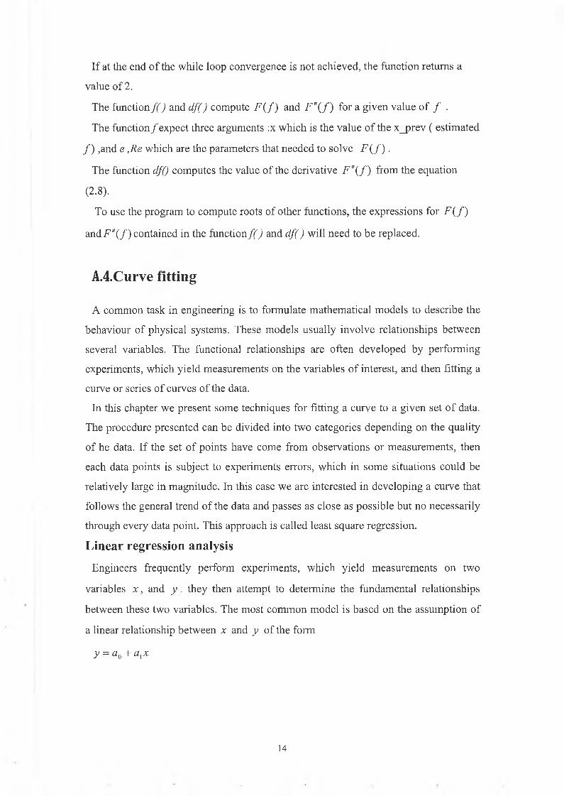
If at the end o f the while loop convergence is not achieved, the function returns a

value o f 2.

The functionf ( ) and df() compute F ( f ) and F"(f) for a given value o f / .

The function/ expect three arguments :x which is the value o f the x_prev ( estimated

/ ) ,and e ,Re which are the parameters that needed to solve F( f ) .

The function df() computes the value o f the derivative F"(f ) from the equation

(2 .8).

To use the program to compute roots o f other functions, the expressions for F { f )

and F"(f) contained in the function f ( ) and df() will need to be replaced.

A.4.Curve fitting

A common task in engineering is to formulate mathematical m odels to describe the

behaviour o f physical systems. These models usually involve relationships between

several variables. The functional relationships are often developed by performing

experiments, which yield measurements on the variables o f interest, and then fitting a

curve or series o f curves o f the data.

In this chapter w e present some techniques for fitting a curve to a given set o f data.

The procedure presented can be divided into two categories depending on the quality

o f he data. If the set o f points have come from observations or measurements, then

each data points is subject to experiments errors, which in som e situations could be

relatively large in magnitude. In this case w e are interested in developing a curve that

follows the general trend o f the data and passes as close as possible but no necessarily

through every data point. This approach is called least square regression.

Linear regression analysis

Engineers frequently perform experiments, which yield measurements on two

variables x , and y . they then attempt to determine the fundamental relationships

between these two variables. The most common m odel is based on the assumption o f

a linear relationship between x and y o f the form

y = a0 + axx

14

points(x, , y {\ {x 2 , y2\ ....., (xn ,y„)- The values o f a0 and a, are determined so that the

straight line passes through the data points with the least errors.

The most w idely used technique for fitting a line through a series o f observed data

points is the least square method.

The basis for the method is represented graphically in Figure A4.1. The calculated

(or predicted) values are given by

y = a0 + alxi

y

Where a0 is the intercept and a, is the slop of the passing through the data

Figure A.4.1 regression line and error associated with point {xn y t) .

W e can extend the least square method to fit a second-, third-, and higher-order

polynomial to the given data set. This is useful for situations where the functional

relationship is non-linear and linearization is not possible. The regression coefficients

are chosen so as to m inim ise the sum o f the squares o f the deviations between the

predicted values and the experimental values.

For the problem o f fitting a second-order polynom ial o f the form

y(x) = a0 + a, + a2 x 2

The corresponding deviation o f the point from the curve is

y t + y i - y i - (°o + x, + a2xf )

And the sum o f the squares o f the deviations is

ns = T J( i ~ ao

/=i

Notice that S is a function o f the three variables, a0 ,an and a2. W e need to take the

partial derivatives o f S with respect to these three variables and set them equal to

zero, that is

“ . 0 . “ - f t *da0 dat da2

= 0

This yield the follow ing three linear algebraic equations

n n n<y* + « i Z * i + « 2 Z * i 2 = Z ^

m (=i i=i

i=i /=i i=i

«.2X +«,!>,3+«2Zx.4 = t*?y,i=i <=1 /=i

The solution o f these equations can be written in matrix form as

n Zx- Z*? V ' z* 'Z* Z*J Z*.3 a l = Zm_Z*2/ Z*? Z*<4__a2 _Z**-2.

(A4, la)

The coefficients o f the polynomial are calculated by solving the above system o f

equations by using Gauss elimination technique.

16

program for polynomial least squares curves fitting

A program to determine the best-fit polynom ial o f degree N to a set o f n data is

shown in appendix B .

The important variables needed to implement polynomial least squares curve fitting

analysis on a computer are the following:

Variables

Number o f data points ( int num. jo in ts )

Arrays for xi and y i values {double x[ ] , Y [ ] )

Degree o f polynom ial ( int num jpoly )

Polynomial coefficients ( double a [ ] )

Algorithm for main

The algorithm for polynomial least square method is as follow:

1. read in the number o f data points {num jo in ts )

2. read in the degree o f the polynomial ( num_poly)

3. read x [ ] and y [ ] arrays

Algorithm fo r poly_leastsqr function

1. Compute the sums o f products

1.1 Initialise S [0] to num_points

1.2 For i = 1 to 2*num_poly

1.2.1 set S[0] to zero

1.2.2 from j = 0 to num jo in ts

1.2.3 calculate S\i] = x\j]

2.Creat coefficient matrix c[z] [/]

3.Creat right-hand side vector

4. Call Gauss elimination function for the solution o f simultaneous equations

17

5.return the result

5.1 return to 0 if the computation is successful

5.2 return to 1 i f coefficient matrix is singular

5.3 return to 2 if the equations are ill conditioned

program

The computations are performed by a separate function called poly-leastsqr (). This

function first assembles the square coefficient matrix and the right hand vector given

in equation (A 4 .la). The coefficient matrix is saved in the two-dim ensional array C [ ]

[ ], and the right-hand vector is saved in the one-dimensional array a [ ]. The function

then calls the Gauss elimination routine (presented in section A 2.1) to solve the

system o f equations to obtain the coefficient o f the best-fit polynom ial.

The function polyjeastsqr ( ) expects five arguments. The array x [ ] and y[ ]

contain the data values (x^yj .the variables num._points represents the number o f

data points, and the variable num_poly represents the degree o f the polynom ial which

is equal to N-l. The function returns the coefficients o f the best-fit polynomial

aN in the array a [ ].

The function creates two local arrays, a one-dimensional array S [ ] and a two-

dimensional array C [ ] [ ] . The array S [ ] used to store the various sums that are

needed to create the coefficient matrix. The elements o f the array S [ ] are obtained

from

W hen n is the number o f data points (represented by the variable num jpoints in the

program). Thus, 5'[l]= *S’[2] = ^ x , 2 , and so on. The first elem ent o f the array

is equal to the number o f data points, n.

The elements o f the coefficient matrix C[ ][ ] are obtained from the array as shown:

S [ K ] = ± x ‘1=1

S[0] S[l] S[2] S[N] S[N + 1]S[l] S[2] S[3]

S[N] S[7V + 1] S[N + 2] S[2N]

18

Where N is the degree o f the polynom ial (represented by the variable num._poly in

the function). The relationship between the elements o f C [ ] [ ] and S [ ] is

C[i][j] = S[i + j]

Thus once the various sums are computed it is a relatively easy task to build the

coefficient matrix C [ ] [ ] .

The right-hand vector is saved in the array a [ ] . The elem ents o f a [ ] are obtained

from

a[K] = ¿ y , j 1=1

The function poly_leastsqr() first creates the arrays S [ ] and a [ ] . It then creates

the array C [] [] by placing the elements o f S [ ] in their appropriate positions in C [ ] [

] . It then calls the function Guass elimination ()

Result=Gauss elimination ( C, a , num_poly+l, & det) ;

To solve the system o f equations. The solution is returned in the array a [ ] . Thus,

upon return, the array a [ ] contains the coefficient o f the best-fit polygon. The

function Guass_elimination() returns a value o f type int indicating the status o f the

computation. Function polyjeastsqr ( ) also returns a value o f type int . The value

returned by polyjeastsqr ( ) is the same value that was returned to it by the function

Guass_elimination().

19

Appendix B

(Computer Program Source Code)

F l o w s i m u l a t i o n . c

/*=================================================================================*//*=================================================================================*//* "WELCOME TO THE PIPE NETWORKS SIMULATION COMPUTER PROGRAM " *//* 11 SCHOOL OF MECHANICAL & MANUFACTURING ENGINEERING 11 *//* DUBLIN CITY UNIVERSITY *//* ( THIS PROGRAM is DEVELOPED BY ) *//* MR. NASSER EMHMMED SALEM KHAMKHAM *//* CHECKED BY PROF. HASHMI SALIM */

/*=================================================================================*/

/ * = = = = = = = = = = = = = = = = = = = = = = = = = = = = = = = = = = = = = = = = = = = = = = = = = = = = = = = = = = = = = = = = = = = = = = = = = = = = = = = = = * /

#include<stdio.h> #include<stdlib.h> #include<math.h>#define MAX_SIZE 150 #define MAXPOINTS 100 #define TRUE 1 #define FALSE 0 #define nearly_zero le-40

void main (void);

/*=================================================================================*/void input(char*file_input);

/*=================================================================================*/void output(char*file_input,char*file_output);

/ * = = = = = = = = = = = = = = = = = = = = = = = = = = = = = = = = = = = = = = = = = = = = = = = = = = = = = = = = = = = = = = = = = = = = = = = = = = = = = = = = = * /

int Linear_Darcy(double QJ[],double QF[],int NP,int NJ,int NL,int JA[],int JB [] , int NNJ; int NN[],int J N [] [MAX_SIZE] , int NPVR,int IFLOW [] , int LP [] [MAX_SIZE] , int LPL[],int NPS,int NLSJ,int LPSL[] ,int LPS [] [MAX_SIZE] ,double A O [],double ELV[],int NUNIT,int NoR,int NPUMP,int NLPUM,int LPUMSL[],int LPUMS[][MAX_SIZE],double HHO [] , double ho [] , double D [] , double E[] , double VIS,double epsilon,double tol,double deq,int max_iter,double KLL[],int NP_PRV[], double L[], double h_loss [], double H_pump [], double QJPV[], double ELT[], double ENGY [], double spg, double H_Jun[], double PRESS[],int p u m p l ine[],double HGL_ELV[] );

/ * = = = = = = = = = = = = = = = = = = = = = = = = = = = = = = = = = = = = = = = = = = = = = = = = = = = = = = = = = = = = = = = = = = = = = = = = = = = = = = = = = * /int Linear Hazen_Williams(double QJ[],int NP,

int NJ,int JA[],int JB[],int NL,int NNJ,int NN[],int JN[] [MAX_SIZE] ,int NPVR, int IFLOW [], int LP[] [MAX_SIZE] , int LPL[],int NPS,int NLSJ,int LPSL[],int LPS[] [MAX_SIZE],double AO[],double ELV[],int NUNIT,int NoR,int NPUMP,int NLPUM,int LPUMSL [] ,int LPUMS[] [MAX_SIZE] ,int NP_PRV [], double HHO [] , double ho[],double CHW[], double KLL [] ,double D [] ,double L[],double tol,int raax_iter,double h_loss[] ,double H_pump[] , double QJPV[] ,double ELT[],double ENGY[],double spg,double H_Jun [], double PRESS [] );

/ * = = = = = = = = = = = = ; = = = = = = = = = = = = = = = = = = = = : : = = = = = = = = = = = = = = = = = = = = = = = = = = = = = = = = = = = = = = = = = = = = = * /

1

int Gauss_elimination (double a[] [MAX_SIZE] ,double b [] ,int n,double *ptr_det);

/ * = = = = = = = = = = = = = = = = = = = = = = = = = = = = = = = = = = = = = = = = = = = = = = = = = = = = = = = = = = = = = = = = = = = = = = = = = = = = = = = = = * /

int Newton_Raphson(double epsilon,double e,double Re,int max_er,double *ptr_fl,int *ptr_numl_iter) ;

int Newton_Raphson2(double fl,double epsilon ,double e,double Re, int max_er,double *ptr_f2,int *ptr_numl_iter);

/ * = = = = = = = = = = = = = = = = = = = = = = = = = = = = = = = = = = = = = = = = = = = = = = = = = = = = = = = = = = = = = = = = = = = = = = = = = = = = = = = = = * /

double f(double x,double e,double Re);

double df(double x,double e,double Re);

/*=================================================================================*/

int poly_leastsqr(double x[],double y[],int num_points,int num_poly ;double ao[]);

/ * = = = = = = = = = = = = = = = = = = = = = = = = = = = = = = = = = = = = = = = = = = = = = = = = = = = = = = = = = = = = = = = = = = = = = = = = = = = = = = = = = * /

/ * = = = = = = = = = = = = = = = = = = = = = = = = = = = = = = = = = = = = = = = = = = = = = = = = = = = = = = = = = = = = = = = = = = = = = = = = = = = = = = = = = * //* function: main() *//* this function main() determines the type of operations to be *//* performed and calls the appropriate computational functions, and display *//* list of choice whether to show all the inputs or to print *//* out the results of the program *// * = = = = = = = = = = = = = = = = = = = = = = = = = = = = = = = = = = = = = = = = = = = = = = = = = = = = = = = = = = = = = = = = = = = = = = = = = = = = = = = = = * /

/ * = = = = = = = = = = = = = = = = = = = = = = = = = = = = = = = = = = = = = = = = = = = = = = = = = = = = = = = = = = = = = = = = = = = = = = = = = = = = = = = = = * /

void main (void )

F l o w _ s i m u l a t i o n . c

printf("\n \t 1- Create a new input file or uptate an existing inputfile ");

char file_input[81]; char file_output[81]; int choice; while(choice!=3){

/* display list of choice */

printf("\n \n \t \t MAIN MENU ");printf("\n \t 1- Create a new input file or uptate an existing iprintf("\n \t 2- shows list of contents of the output file");printf("\n \t 3- Exist the program");

choice=0;while ( choicecl || choice>3){

printf("\n \t your choice (1,2 or 3)?"); scanf("%d",&choice);

}if ( choice!=3){

printf("\n \t Enter the filename of the input file :"); scanf("%s",file_input);printf("\n \t Enter the filename of the output file :"); scanf("%s",file_output); switch(choice)

{case 1:input(file_input); break;

2

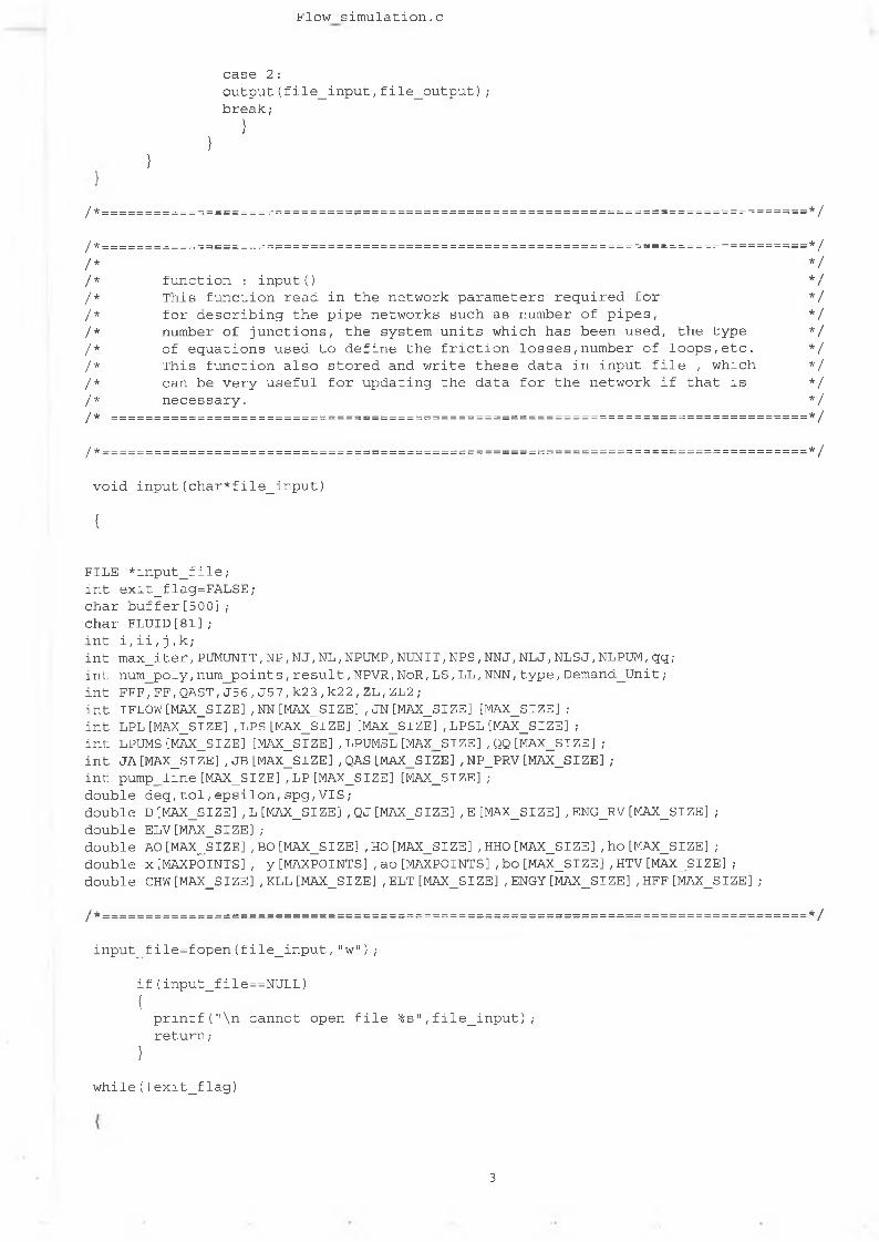
F l o w s i m u l a t i o n . c

case 2 :output(file_input,file_output); break ;

}}

}

/*=================================================================================*/

/*=================================================================================*//* * / /* function : input() *//* This function read in the network parameters required for *//* for describing the pipe networks such as number of pipes, *//* number of junctions, the system units which has been used, the type *//* of equations used to define the friction losses,number of loops,etc. *//* This function also stored and write these data in input file , which *//* can be very useful for updating the data for the network if that is *//* necessary. *// * = = = = = = = = = = = = = = = = = = = = = = = = = = = = = = = = = = = = = = = = = = = = = = = = = = = = = = = = = = = = = = = = = = = = = = = = = = = = = = = = * /

/ * = = = = = = = = = = = = = = = = = = = = = = = = = = = = = = = = = = = = = = = = = = = = = = = = = = = = = = = = = = = = = = = = = = = = = = = = = = = = = = = = = * /

void input(char*file_input)

{

FILE *input_file; int exit_flag=FALSE; char buffer[500]; char FLUID[81] ; int i,ii,j ,k;int max_iter,PUMUNIT,NP,NJ,NL,NPUMP,NUNIT,NPS,NNJ,NLJ,NLSJ,NLPUM,qq; int num_poly,num_points,result,NPVR,NoR,LS,LL,NNN,type,Demand_Unit; int FFF,FF,QAST,J56,J57,k23,k2 2,ZL,ZL2;int IFLOW [MAX_SIZE] ,NN[MAX_SIZE] ,JN[MAX_SIZE] [MAX_SIZE] ; int LPL[MAX_SIZE],LPS[MAX_SIZE][MAX_SIZE],LPSL[MAX_SIZE]; int LPUMS[MAX_SIZE][MAX_SIZE],LPUMSL[MAX_SIZE],QQ[MAX_SIZE]; int JA[MAX_SIZE],JB[MAX_SIZE],QAS[MAX_SIZE],NP_PRV[MAX_SIZE]; int pump_line[MAX_SIZE],LP[MAX_SIZE][MAX_SIZE]; double deq,tol,epsilon,spg,VIS;double D[MAX_SIZE],L[MAX_SIZE],QJ[MAX_SIZE],E[MAX_SIZE],ENG_RV[MAX_SIZE]; double ELV[MAX_SIZE];double AO[MAX_SIZE],BO[MAX_SIZE],HO[MAX_SIZE],HHO[MAX_SIZE],ho[MAX_SIZE]; double x[MAXPOINTS], y[MAXPOINTS],ao[MAXPOINTS],bo[MAX_SIZE],HTV[MAX_SIZE]; double CHW[MAX_SIZE],KLL[MAX_SIZE],ELT[MAX_SIZE],ENGY[MAX_SIZE],HFF[MAX_SIZE];

/* = = = =------- = = == = = = = = = =------------- = = = = = = = = == = = = = = = == = = = = = = = = = == = = = = = = = = = = =--------;= = = = = = = = ==*/

input_file=fopen(file_input,"w");

if (input_file==NULL){printf("\n cannot open file %s11, file_input) ; return;

}

while(!exit_flag)

3

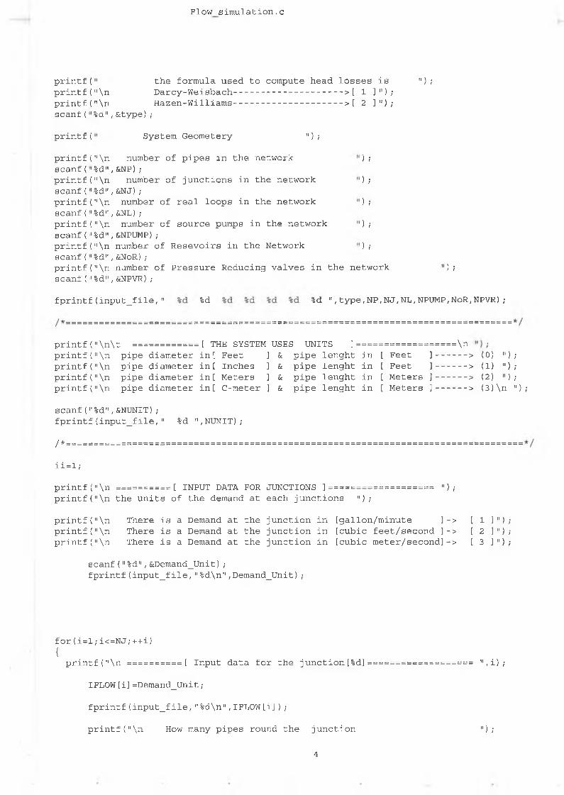
F l o w s i m u l a t i o n . c

printf printf printf scanf(

printf

printf scanf( printf scanf( printf scanf( printf scanf( printf scanf( printf scanf(

11 \n " \n%d",&type);

the formula used to compute head losses isDarcy-Weisbach--------------------- > [ 1 ] ") ;Hazen-Williams--------------------- >[ 2 ]");

") ;

System Geometery ") ;

"\n %d", " \n %d", " \n %d", 11 \n %d", " \n %d", 11 \n %d",

number of pipes in the network &NP) ;

number of junctions in the network &NJ) ;number of real loops in the network &NL) ;number of source pumps in the network &NPUMP);number of Resevoirs in the Network &NoR);number of Pressure Reducing valves in the network &NPVR);

") ;

fprintf(input_file," %d ^d ",type,NP,NJ,NL,NPUMP,NoR,NPVR);

printf("\n\t ============[ THE SYSTEM USES UNITS ]printf("\n pipe diameter int Feet ]printf("\n pipe diameter in [ Inches ]printf (11 \n pipe diameter in [ Meters ]printf("\n pipe diameter in[ C-meter ]

=\n& pipe lenght in [ Feet ]-------> (0) ")& pipe lenght in [ Feet )-------> (1) ")& pipe lenght in [ Meters ]-------> (2) 11 )& pipe lenght in [ Meters ]-------> (3)\n ");

scanf("%d",&NUNIT) ; fprintf (input_file, 11 %d ",NUNIT);

/* =

i i=1 ;

printf("\n ==========[ INPUT DATA FOR JUNCTIONS ]========:printf("\n the units of the demand at each junctions ");

") ;

printf("\n There is a Demand at the junction in [gallon/minute ]-> [ 1 ]"}printf("\n There is a Demand at the junction in [cubic feet/second ]-> [ 2 )")printf("\n There is a Demand at the junction in [cubic meter/second]-> [ 3 ]")

scanf("%d",&Demand_Unit);fprintf(input_file,"%d\n",Demand_Unit);

for(i=l;i<=NJ;++i){printf("\n ==========[ Input data for the junction[%d]=================== ",i);

IFLOW[i]=Demand_Unit;

fprintf(input_file,"%d\n",IFLOW[i]);

printf ("\n How many pipes round the junction 11) ;

4

F l o w s i m u l a t i o n . c

scanf (11 %d", &NNJ)fprintf(input_file,"%d \n",NNJ);

for (j=1;j<=NNJ;++j){

printf("\n Number of the pipe at junction ");

printf("\n if flow Leaves the junction -----> The pipe Number is [ + ]");printf("\n if flow Enters the junction----- > The pipe Number is [ - ]");scanf("%d",&JN[i][ j ] ) ;fprintf(input_file,"%d \n",JN[i][j]);

}NN[i]=NNJ;fprintf(input_file,"%d \n",NN[i]);

if (IFLOW[i]==1){

printf("\n The flow rates in [ GPM ] ");scanf (11 %lf " , &QJ [ii] ) ;

QJ [ii]=QJ[ii]/449.0;fprintf(input_file,"%lf\n",QJ[ii] ) ;ii=ii+l;

}if(IFLOW[i]==2){

printf("\n The Flow rate in [ CFS ]scanf ("%lf11, &QJ [ii] ) ; fprintf(input_file,"%lf\n",QJ[ii]); ii=ii+l;

}if(IFLOW [i]= = 3)

{printfC'\n The Flow rate in [ CMS ] ");scanf ("%lf11, &QJ [ii] ) ;fprintf(input_file,"%lf\n",QJ[ii]);ii=ii+l;

}

printf("\n THE ELEVATION OF THE JUNCTIONscanf("%lf",&ELT[i]); fprintf(input_file,"%lf\n",ELT[i]);

for(i=l;i<=NJ;++i){

NNJ=NN[i];}

/*=================================================================================*/

tol=0.000001;

fprintf(input_file,"%lf ",tol);

/ * = = = = = = = = = = = = = = = = = = = = = = = = = = = = = = = = = = = = = = = = = = = = = = = = = = = = = = = = = = = = = = = = = = = = = = = = = = = = = = = = = * /

if(type==l)

5

F l o w s i m u l a t i o n . c

printf("\n =========THE FLUID PROPERTIES =============== ") ;

printf ( " \n\t TYPE OF FLUID ");scanf("%s",FLUID); fprintf(input_file,"%s ", FLUID) ;printf("\n\t THE FLUID VISCOSITY ");scanf("%g",&VIS);fprintf(input_file,"%g ",VIS);printf("\n\t THE FLUID SPECIFIC GRAVITY ");scanf("%lf",&spg);fprintf (input_file, "%lf ", spg) ,-epsilon=0.001;fprintf(input_file,"%lf \n",epsilon); deq=0.1;fprintf(input_file,"%lf \n",deq);

for(i=l;i<=NP;++i){printf("\n Pipe [%d]",i);

printf("\n node no 1 connects the pipe");scanf("%d",&JA[i]);fprintf(input_file,"%d ",JA[i]);printf("\n node no 2 connects the pipe");scanf("%d",&JB[i]);fprintf(input_file,"%d ",JB[i]);printf("\n Pipe Diameter ");scanf("%lf",&D[i]);fprintf(input_file,"%lf ",D [i]) ;printf("\n Pipe Lenght ");scanf("%lf",&L [i]);fprintf(input_file,"%lf ",L [i]);printf("\n Relative roughness of pipe ");scanf("%lf",&E[i]);fprintf(input_file,"%lf ",E [i]) ;printf("\n Minor Lose Coefficient ");scanf("%lf",&KLL[i]);fprintf(input_file,"%lf ",KLL[i]);

/ ’

if(type==2){

for(i=l;i<=NP;++i){

printf("\n Pipe [%d]",i);printf("\n node no 1 connects the pipe");scanf("%d",&JA[i]);fprintf(input_file,"%d ",JA[i]);printf("\n node no 2 connects the pipe");scanf("%d",&JB [i]) ;fprintf(input_file,"%d ",JB [i]);printf("\n Pipe Diameter in ");scanf("%lf",&D [i]) ;fprintf(input_file,"%lf ",D[i]);printf("\n Pipe Lenght in ");scanf("%lf",&L [i]) ;

6

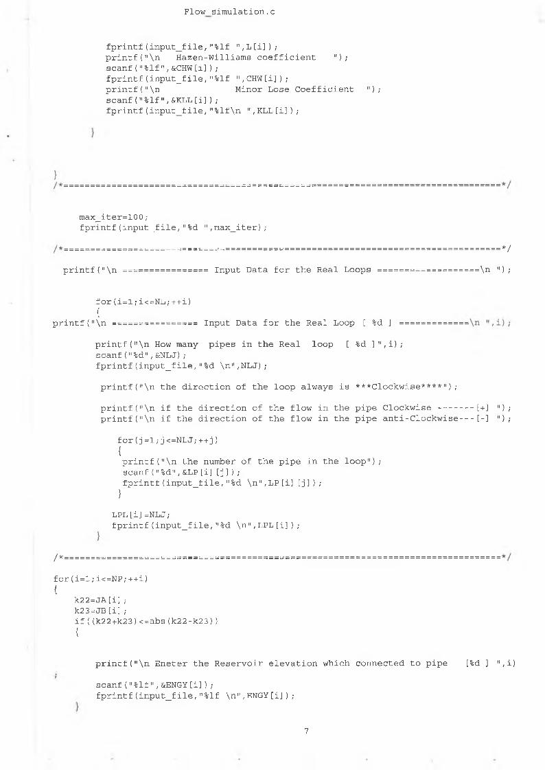
F l o w s i m u l a t i o n . c

fprintf(input_file,"%lf ",L[i]);printf("\n Hazen-Williams coefficient ");scanf("%lf",&CHW[i]);fprintf (input_file, "%lf 11, CHW [i] ) ;printf("\n Minor Lose Coefficient ");scanf("%lf",&KLL[i]);fprintf(input_file,"%lf\n ",KLL[i]);

max_iter=10 0;fprintf(input_file,"%d ",max_iter);

printf("\n ================ Input Data for the Real Loops

=====*/

An ") ;

for(i = l;i < =NL;+ + i) {

printf("\n Input Data for the Real Loop [ %d ]

/*=

printf("\n How many pipes in the Real loop [ %d ]",i);scanf("%d",&NLJ);fprintf(input_file,"%d \n",NLJ);

printf("\n the direction of the loop always is ***Clockwise****");

printf("\n if the direction of the flow in the pipe Clockwise --------[+] ");printf(M\n if the direction of the flow in the pipe anti-Clockwise---- [-] ");

for(j =1;j <=NLJ;+ + j){printf(n\n the number of the pipe in the loop"); scanf("%d",&LP[i][j]);fprintf(input_file,"%d \n",LP[i][j]);

}

LPL[i]=NLJ;fprintf(input_file,"%d \n",LPL [i]) ;

for ( i = l ; i < = N P ; + + i )

{k22=JA[i]; k23=JB[i];if((k22+k23)<=abs(k22-k23)) {

printf("\n Eneter the Reservoir elevation which connected to pipe [%d ] ",i)

scanf (11 %lf" , &ENGY [i] ) ;fprintf(input_file,"%lf \n",ENGY[i]);

7

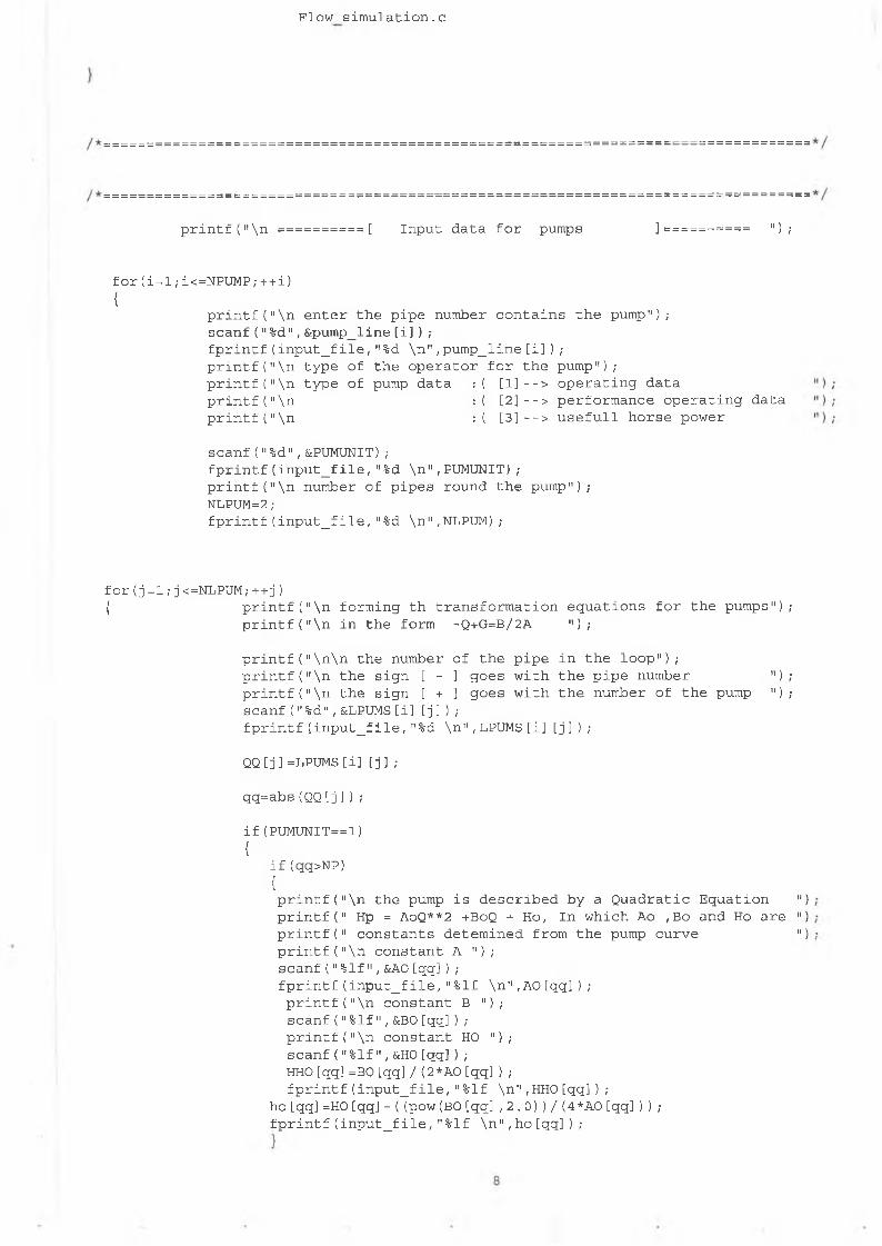
F l o w s i m u l a t i o n . c

printf("\n ==========[ Input data for pumps ]========== ");

for(i=l;i<=NPUMP;++i){

printf("\n enter the pipe number contains the pump");scanf("%d",&pump_line[i]),-fprintf(input_file,"%d \n",pump_line[i]);printf("\n type of the operator for the pump");printf("\n type of pump data :( [l]--> operating dataprintf("\n :( [2]--> performance operating dataprintf("\n :( [3]--> usefull horse power

scanf (11 %d" , &PUMUNIT) ;fprintf(input_file,"%d \n",PUMUNIT);printf("\n number of pipes round the pump");NLPUM=2;fprintf(input_file,"%d \n",NLPUM);

for(j =1;j <=NLPUM;++j){ printf("\n forming th transformation equations for the pumps");

printf("\n in the form -Q+G=B/2A ");

printf("\n\n the number of the pipe in the loop");printf("\n the sign [ - ] goes with the pipe number ");printf("\n the sign [ + ] goes with the number of the pump ");scanf("%d",&LPUMS[i][j]); fprintf(input_file,"%d \n",LPUMS[i][j]);

QQ[j] =LPUMS [i] [j] ;

qq=abs(QQ[j]);

if(PUMUNIT==1){

if(qq>NP){printf("\n the pump is described by a Quadratic Equation ") printf(" Hp = AoQ**2 +BoQ + Ho, In which Ao ,Bo and Ho are ") printf (11 constants detemined from the pump curve ")printf("\n constant A "); scanf("%lf", &A0[qq]) ; fprintf(input_file,"%lf \n",AO[qq]); printf("\n constant B "); scanf("%lf",&B0[qq]); printf("\n constant HO "); scanf("%lf",&H0[qq]);HHO[qq]=B0[qq]/ (2*A0[qq]); fprintf(input_file,"%lf \n",HHO[qq]);

ho[qq]=H0[qq]-((pow(BO[qq],2.0))/(4*AO[qq])); fprintf(input_file,"%lf \n",ho[qq]);

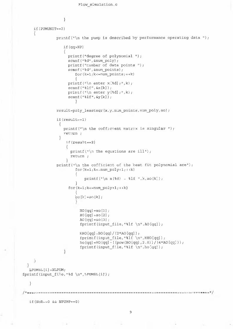
F l o w s i m u l a t i o n . c

}

if(PUMUNIT==2) {

printf("\n the pump is described by performance operating data ");

if(qq>NP){printf("degree of polynomial "); scanf("%d",&num_poly); printf("number of data points "); scanf("%d",&num_points);

for(k=l;k<=num_points;++k){

printf("\n enter x[%d];",k); scanf("%lf",&x[k]); printf("\n enter y[%d];",k); scanf("%lf",&y[k]);

}

result=poly_leastsqr(x,y,num_points,num_poly,ao);

if(result==l){printf("\n the cofficient matrix is singular "); return ;

}if(result==2){printf("\n The equations are ill"); return ;

}printf("\n the cofficient of the best fit polynomial are");

for(k=l;k<=num_poly+l;++k){

printf("\n a(%d) = %lf ",k,ao[k]);}

for(k=l;k<=num_poly+l;++k){bo[k]=ao[k];

HO[qq]=ao [1] ;BO[qq]=ao [2] ;AO[qq]=ao [3] ;fprintf(input_file,"%lf \n",AO[qq]);

HHO[qq]=B0[qq]/ (2*A0[qq]);fprintf(input_file,"%lf \n",HHO[qq]);ho [qq] =H0 [qq] - ( (pow (BO [qq] ,2.0))/ (4*AO [qq] ) ) ;fprintf(input_file,"%lf \n",ho[qq]);

}}LPUMSL[i]=NLPUM;

fprintf(input_file,"%d \n",LPUMSL[i]);

}

if (NoR= = 0 ScSc NPUMP= = 0 )

9

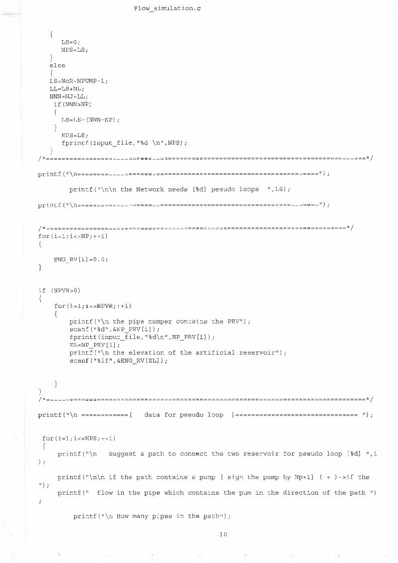
F l o w s i m u l a t i o n . c

{LS = 0 ;NPS=LS;

}else{LS=NoR+NPUMP-l;LL=LS+NL;NNN=NJ+LL; if(NNN>NP){LS=LS-(NNN-NP);

}NPS=LS;fprintf(input_file,"%d \n",NPS);

}/ * = = = = = = = = = = = = = = = = = = = = = = = = = = = = = = = = = = = = = = = = = = = = = = = = = = = = = = = = = = = = = = = = = = = = = = = = = = = = = = = = = * /

printf("\n=============================================================");

printf("\n\n the Network needs [%d] pesudo loops ",LS);

printf("\n=============================================================");

/*============================================================================*/for(i=1;i<=NP;++i){

ENG_RV[i]= 0.0;}

if (NPVR>0){

for(i=l;i<=NPVR;++i){

printf (11 \n the pipe numper contains the PRV");scanf("%d",&NP_PRV[i]);fprintf(input_file,"%d\n",NP_PRV[i]);ZL=NP_PRV[i];printf("\n the elevation of the artificial reservoir"); scanf("%lf",&ENG R V [ZL]);

}/ * = = = = = = = = = = = = = = = = = = = = = = = = = = = = = = = = = = = = = = = = = = = = = = = = = = = = = = = = = = = = = = = = = = = = = = = = = = = = = = = = = * /

printf("\n ============[ data for pseudo loop ]=============================== ");

for(i=l;i<=NPS;++i){

printf("\n Suggest a path to connect the two reservoir for pseudo loop [%d] ",i) ;

printf("\n\n if the path contains a pump [ sign the pump by Np+1] ( + )->if the") ;

printf(" flow in the pipe which contains the pum in the direction of the path ")

printf("\n How many pipes in the path");

10

F l o w s i m u l a t i o n . c

scanf("%d",&NLS J);fprintf(input_file,"%d \n",NLSJ);

HFF[i]=0.0;

for(j=l; j <=NLSJ; + +j ){

printf<"\n the number of the pipe in the loop");printf("\n [ + ] if flow in the same direction of the energy line ");printf("\n [ - ] if flow oppesite the energy line direction ");scanf("%d",&LPS[i][j]); fprintf(input_file,"%d \n",LPS[i][j]);

LPSL[i]=NLSJ;fprintf(input_file,"%d \n",LPSL[i]);

FFF=LPS[i][1];FF=abs(FFF);

QAS[j]=LPS[i] [j] ;

QAST=abs(QAS[j]);

if(QAST<=NP){

J56=JA[QAST];

J57=JB[QAST];

if((J56+J57)<=abs(J56-J57)){if(QAST==FF){

HTV[1]=ENGY[QAST];

}else

{HTV[2]=ENGY[QAST];

}

}if(NPVR>0){

for(k=l;k<=NPVR;++k) {

ZL2=NP_PRV[k];if(ZL2==QAST){

H T V [ 2 ] = E N G _ R V [ Z L 2 ] ;

}}

}

if(QAST>NP)

11

{

if(QAS[j]>0){

HFF[i] =HFF[i]-ho[QAST] ;

>else{

HFF[i] =HFF[i]+ho[QAST] ;

}}

}

ELV[i]=HTV[1]-HTV[2]+HFF [ i] ;

fprintf(input_file,"%lf \n",ELV[i]);

/ * = = = = = = = = = = = = = = = = = = = = = = = = = = = = = = = = = = = = = ;= = = = = = = = = = = = = = = = = = = = = = = = = = = = = = = = = = = = = = - ^ = = = * /

printf("\n do u want to enter more data- Y/N? " );

scanf("%s",buffer);

if ( buffer[0]=='N' ||buffer[0]==1n ') exit_flag=TRUE;

fclose(input_file);

} /* end of the main function void(char filename) */

/ * =================================================================================*/

/*==============================================================================*//* function : output() *// * * //* This function reads in the data for the network from the function *//* inputO. Also prints the result of the program. *//* This function has two sub-functions, function Linear_Darcy() if the *//* Darcy equations is used to define the friction losses, and function *//* Linear_Hazen_William() if the Hazen-William equations is used. *// * * // * * //*==============================================================================*/

Flow_simulation.c

12

Flow simulation.c

/ * = = = = = = = = = = = = = = = = = = = = = = = = = = = = = = = = = = = = = = = = = = =

void output(char*file_input,char*file_output)

{

FILE *outfile;FILE *input_file; int exit_flag=FALSE; char FLUID[81];

int i , j , i i ;int NP,NJ,NL,NPUMP,NoR,type,NUNIT,NPVR,result; int max_iter,PUMUNIT,NPS,NNJ,NLJ,NLSJ,NLPUM,qq; int k22,k2 3,npt2,Demand_Unit;int IFLOW[MAX_SIZE],NN[MAX_SIZE],JN[MAX_SIZE][MAX_SIZE],LP[MAX_SIZE][MAX_SIZE];int LPL [MAX_SIZE] ,LPS[MAX_SIZE] [MAX_SIZE] ,LPSL[MAX_SIZE] ;int LPUMS [MAX_SIZE] [MAX_SIZE] ,LPUMSL[MAX_SIZE] ,QQ[MAX_SIZE] ;int JA[MAX_SIZE],JB[MAX_SIZE],NP_PRV[MAX_SIZE],pump_line[MAX_SIZE];

double tol,deq,epsilon,spg,VIS;double QF[MAX_SIZE],D[MAX_SIZE],L[MAX_SIZE],E[MAX_SIZE],QJPV[MAX_SIZE]; double KLL[MAX_SIZE],h_loss[MAX_SIZE],H_pump[MAX_SIZE],H_Jun[MAX_SIZE]; double AO[MAX_SIZE],ELV[MAX__SIZE],CHW[MAX^SIZE],PRESS[MAX_SIZE]; double HHO[MAX_SIZE],ho[MAX_SIZE],ELT[MAX_SIZE],EMGY[MAX_SIZE]; double HGL ELV[MAX SIZE],QJ[MAX_SIZE];

/ * ===== = = = = = =========C==========:========= = === = = = === ============_=II======= = =====*/

input_file=fopen(file_input,Mr");

if(input_file==NULL){

printf("\n cannot open file %s",file_input); return;

}

outfile=fopen(file_output,"w");

if(outfile==NULL){printf("\n cannot open file %s",file_output); return;

}

fscanf(input_file," %d %d %d %d %d %d %d ",&type,&NP,&NJ,&NL,&NPUMP,&NoR,&NPVR);

fscanf(input_file," %d ",&NUNIT);

ii = l;

13

Flow simulation.c

fscanf(input_file,"%d \n",&Demand_Unit); for(i=l;i<=NJ;++i){

fscanf(input_file,"%d\n",& I F L O W [i]) ; fscanf(input_file,"%d \n",&NNJ);

for (j=l;j<=NNJ;++j){ '

fscanf(input_file,"%d \n",&JN[i][j]);}

NN[i]=NNJ; fscanf{input_file,"%d \n",&NN[i]); if (IFLOW[i]==1){

fscanf(input^file,"%lf\n",&QJ[ii]); ii=.ii+l;

}if(IFLOW[i]==2){

fscanf(input_file,"%lf\n",&QJ[ii]); ii=ii+l;

}if(IFLOW[i]==3)

{

fscanf (input_file, 11 %lf\n" , &QJ [ii] ) ; ii=ii+l;

}

fscanf(input_file,"%lf\n",&ELT[i]);

}

for(i=l;i<=NJ;++i) {

N N J = N N [ i ] ;}

fscanf(input_file,"%lf ",&tol);

/ * ===================;==============================================================* /

if(type==l){

fscanf(input_file,"%s ",FLUID);

fscanf(input_file,"%lf ",&VIS) ;

fscanf(input_file,"%lf ",&spg);

fscanf(input_file,"%lf \n",&epsilon);

1 4

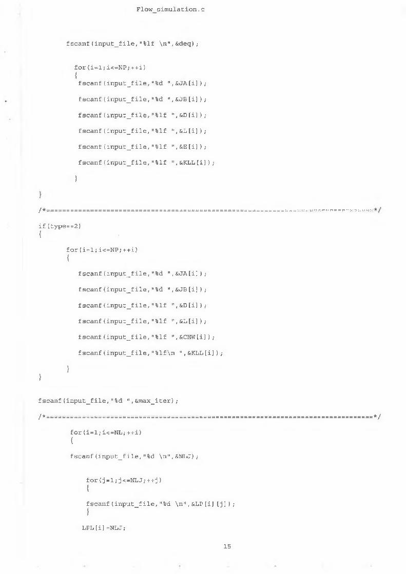
Flow simulation.c

fscanf(input_file,"%lf \n",&deq);

for(i=l;i<=NP;++i){fscanf(input_file,"%d ",&JA[i]);

fscanf(input_file,"%d ",&JB [i]);

fscanf(input_file,"%lf ",&D[i]);

fscanf(input_file,"%lf ",&L[i]);

fscanf(input_file,"%lf ",&E[i]);

fscanf(input_file,"%lf ",&KLL[i]);

)

h

if(type==2)I

for(i=l;i<=NP;++i)i

fscanf(input_file,"%d ",&JA[i]);

fscanf(input_file,"%d ",&JB[i]);

fscanf(input_file,"%lf ",&D[i]);

fscanf(input_file,"%lf ",&L[i]);

fscanf (input_file, "%lf ",ScCHW[i] ) ;

fscanf(input_file,"%lf\n ",&KLL[i]);

}|

fscanf(input_file,"%d ",&max_iter);

/ * = = = = = = = = = = = = = = = = = = = = = = = = = = = = = = = = = = = = = = = = = = = = = = = = = = = = = = = = = = = = = = = = = = = = = = = = = = = = = = = = = * /

for(i=l;i<=NL;++i){

fscanf(input_file,"%d \n",&NLJ);

for(j =1;j <=NLJ;++j){

fscanf(input_file,"%d \n",&LP[i][j]);I

LPL[i]=NLJ;

1 5

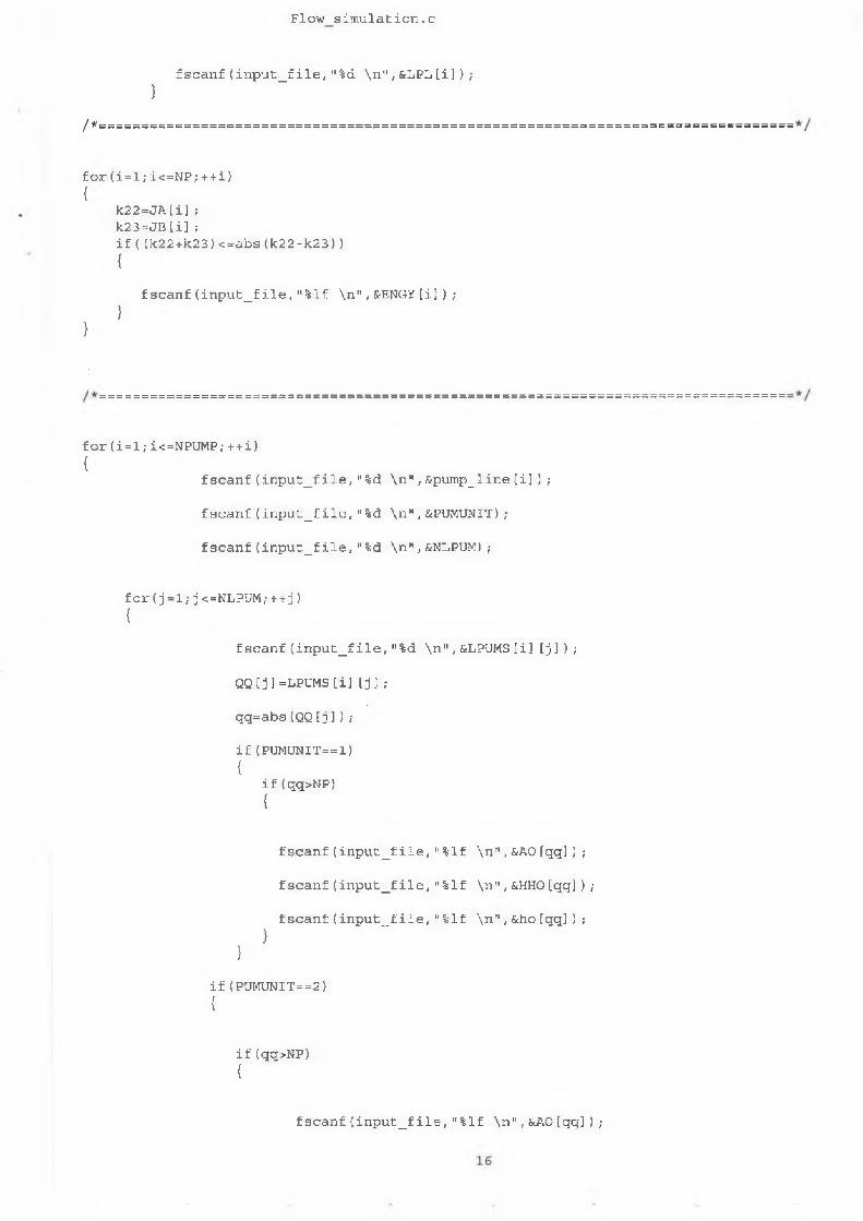
Flow simulation.c

fscanf(input_file,"%d \n",&LPL[i]);i

/*=

for(i=l;i<=NP;++i)I

k 2 2 = J A [i]; k 2 3 = J B [ i ] ;if( ( k 2 2 + k 2 3 ) <=abs ( k 2 2 - k 2 3 ) ){

fscanf (input_file, "%lf \n" , ScENGY [i] ) ;}

}

for(i=l;i<=NPUMP;++i){

fscanf(input_file,"%d \n",&pump_line[i]);

fscanf(input_file,"%d \n",&PUMUNIT);

fscanf(input_file,"%d \n",&NLPUM);

for(j =1;j <=NLPUM;+ +j){

fscanf(input_file,"%d \n",&LPUMS[i][j]);

QQ[j]=LPUMS[i] [j] ;

qq=abs(QQ[j] ) ;

if(PUMUNIT==1)1

if(qq>NP){

fscanf(input_file,"%lf \n",&AO[qq]);

fscanf(input_file,"%lf \n",&HHO tqq]);

fscanf(input_file,"%lf \n",&ho[qq]);

}}

if(PUMUNIT==2) {

if(qq>NP){

fscanf (input_f ile, "%lf \n", ScAO [qq] ) ;

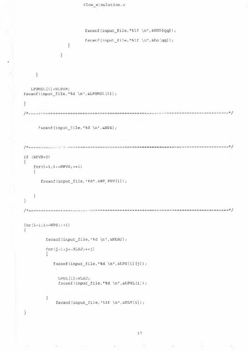
Flow simulation.c

f s c a n f ( i n p u t _ f i l e , " % l f \ n " , & H H O [ q q ] ) ;

f s c a n f ( i n p u t _ f i l e , " % l f \ n " , & h o tqq]);

L P U M S L [ i ] = N L P U M ; f s c a n f ( i n p u t _ f i l e , " % d \ n " , & L P U M S L [ i ] ) ;

f s c a n f ( i n p u t _ f i l e , " % d \ n " , & N P S ) ;

i f ( N P V R > 0 ){

f o r ( i = l ; i < = N P V R ; + + i ){

f s c a n f ( i n p u t _ f i l e , " %d" , & N P _ P R V [ i ] ) ;

}}

/ * = = = = = = = = = = = = = = = = = = = = = = = = = = = = = = = = = = = = = = = = :

f o r ( i = l ; i < = N P S ; + + i ) {

f s c a n f ( i n p u t _ f i l e , " % d \ n " , & N L S J ) ;

f o r ( j = l ; j < = N L S J ; + + j ){

f s c a n f ( i n p u t _ f i l e , " % d \ n " , S t L P S [ i ] [ j ] ) ;

L P S L [ i ] = N L S J ;f s c a n f ( i n p u t _ f i l e , " % d \ n " , & L P S L [ i ] ) ;

f s c a n f ( i n p u t _ f i l e , " % l f \ n " , & E L V [ i ] ) ;1

1 7

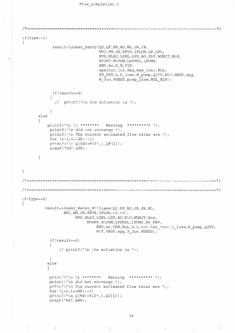
Flow simulation.c

/ * = = = = = = = = =

if(type==l) {

result=Linear_Darcy(QJ,QF,NP,NJ,NL,JA,JB,NN J ,NN,JN,NPVR,IFLOW,LP,LPL,NPS,NLSJ,LPSL,LPS,AO,ELV,NUNIT,NoR,NPUMP,NLPUM,LPUMSL,LPUMS,HHO,ho,D,E,VIS,epsilon,tol,deq,max_iter,KLL,NP_PRV, L, h_JLoss ,H_pump, QJPV, ELT, ENGY, spg, H_Jun,PRESS,pump_line,HGL_ELV);

if(result==0){

// printf("\n the soluation is ");

}else{

printf("\n \t ******** Warning ********** ") ; printf("\n did not converge ");printf("\n The current estimated flow rates are 11) ;for (i=l;i<=NP;++i)printf("\n Q(%d)=%lf",i,QF [i]) ;scanf("%d",&NP);

}

/ * = = = = = = = = = = = = = = = = = = = = = = = = = = = = = = = = = = = = = = = = = = = = = = = = = = = = = = = = = = = = = = = = = = = = = = = = = = = = = = = = = * /

/ * = = = = = = = = = = = = = = = = = = = = = = = = = = = = = = = = = = = = = = = = = = = = = = = = = = = = = = = = = = = = = = = = = = = = = = = = = = = = = = = = = * /

if(type==2){

result=Linear_Hazen_Williams(QJ,NP,NJ,JA,JB,NL,NNJ,NN,JN,NPVR,IFLOW,LP,LPL,

NPS,NLSJ,LPSL,LPS,AO,ELV,NUNIT,NoR,NPUMP,NLPUM,LPUMSL,LPUMS,NP_PRV,

HHO,ho,CHW,KLL,D,L,tol,max_iter,h_loss,H_pump,QJPV, ELT,ENGY,spg,H_Jun,PRESS);

if(result==0){

// printf("\n the soluation is ");

}else{

printf("\n \t ******** Warning ********** "); printf("\n did not converge ");printf("\n The current estimated flow rates are ");for (i = 1;i< =NP;++i)printf("\n Q(%d)=%lf",i,QJ[i]);scanf("%d",&NP);

1 8

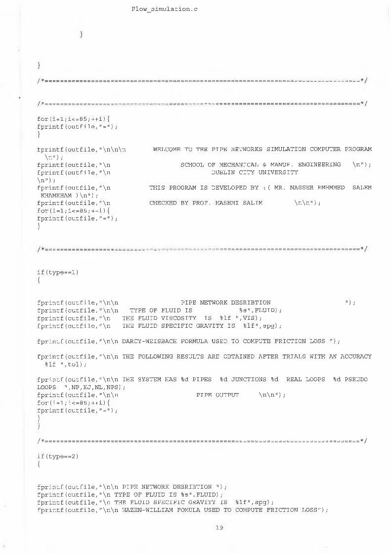
Flow simulation.c

/ * =

/ * -

f o r ( i = l ; i < = 8 5 ; + + i ) { f p r i n t f ( o u t f i l e , " = " ) ;

}

f p r i n t f ( o u t f i l e , " \ n \ n \ n \ n " ) ;

f p r i n t f ( o u t f i l e , " \ n f p r i n t f ( o u t f i l e , " \ n \ n " ) ;f p r i n t f ( o u t f i l e , " \ n

KHAMKHAM ) \ n " ) ; f p r i n t f ( o u t f i l e , " \ n f o r ( i = l ; i < = 8 5 ; + + i ) { f p r i n t f ( o u t f i l e , " = " ) ;

}

==*/

WELCOME TO THE P I P E NETWORKS SIMULATION COMPUTER PROGRAM

SCHOOL OF MECHANICAL & MANUF. ENGINEERING \ n " ) ; DUBLIN C I T Y U N I V E R S I T Y

T H IS PROGRAM I S DEVELOPED BY : ( MR. NASS ER EMHMMED SALEM

CHECKED BY PROF. HASHMI SAL IM \ n \ n " ) ;

i f ( t y p e = = l )

{

f p r i n t f ( o u t f i l e , " \ n \ n P I P E NETWORK D E SR IB T IO N " ) ;f p r i n t f ( o u t f i l e , " \ n \ n TYPE OF FLUI D I S % s 11 , FLUI D) ;f p r i n t f ( o u t f i l e , " \ n THE FLUID V I S C O S I T Y I S % l f " , V I S ) ; f p r i n t f ( o u t f i l e , " \ n THE FLUI D S P E C I F I C GRAVI TY I S % l f " , s p g ) ;

f p r i n t f ( o u t f i l e , " \ n \ n DARCY- WEISBACH FORMULA USED TO COMPUTE F R I C T I O N LOSS " ) ;

f p r i n t f ( o u t f i l e , " \ n \ n THE FOLLOWING R ESULTS ARE OBTAINED AF T ER T R I A L S WITH AN ACCURACY % l f 11 , t o l ) ;

f p r i n t f ( o u t f i l e , " \ n \ n THE SYSTEM HAS %d P I P E S %d JUNCTIONS %d REAL LOOPS %d PSEUDO LOOPS " , N P , N J , N L , N P S ) ;f p r i n t f ( o u t f i l e , " \ n \ n P I P E OUTPUT \ n \ n " ) ;f o r ( i = l ; i < = 8 5 ; + + i ) { f p r i n t f ( o u t f i l e , " = " ) ;

}

/ * = = = = = = = = = = = = = = = = = = = = = = = = = = = = = = = = = = = = = = = = = = = = = = = = = = = = = = = = = = = = = = = = = = = = = = = = = = = = = = = = = * /

i f ( t y p e = = 2 )

{

f p r i n t f ( o u t f i l e , " \ n \ n p i p e NETWORK DE SRIBT ION " ) ;f p r i n t f ( o u t f i l e , " \ n TYPE OF FLUI D I S % s " , F L U I D ) ;f p r i n t f ( o u t f i l e , " \ n THE FLUID S P E C I F I C GRAVI TY I S % l f " , s p g ) ;f p r i n t f ( o u t f i l e , " \ n \ n HAZEN-WILLIAM FOMULA USED TO COMPUTE F R I C T I O N L O S S " ) ;

19

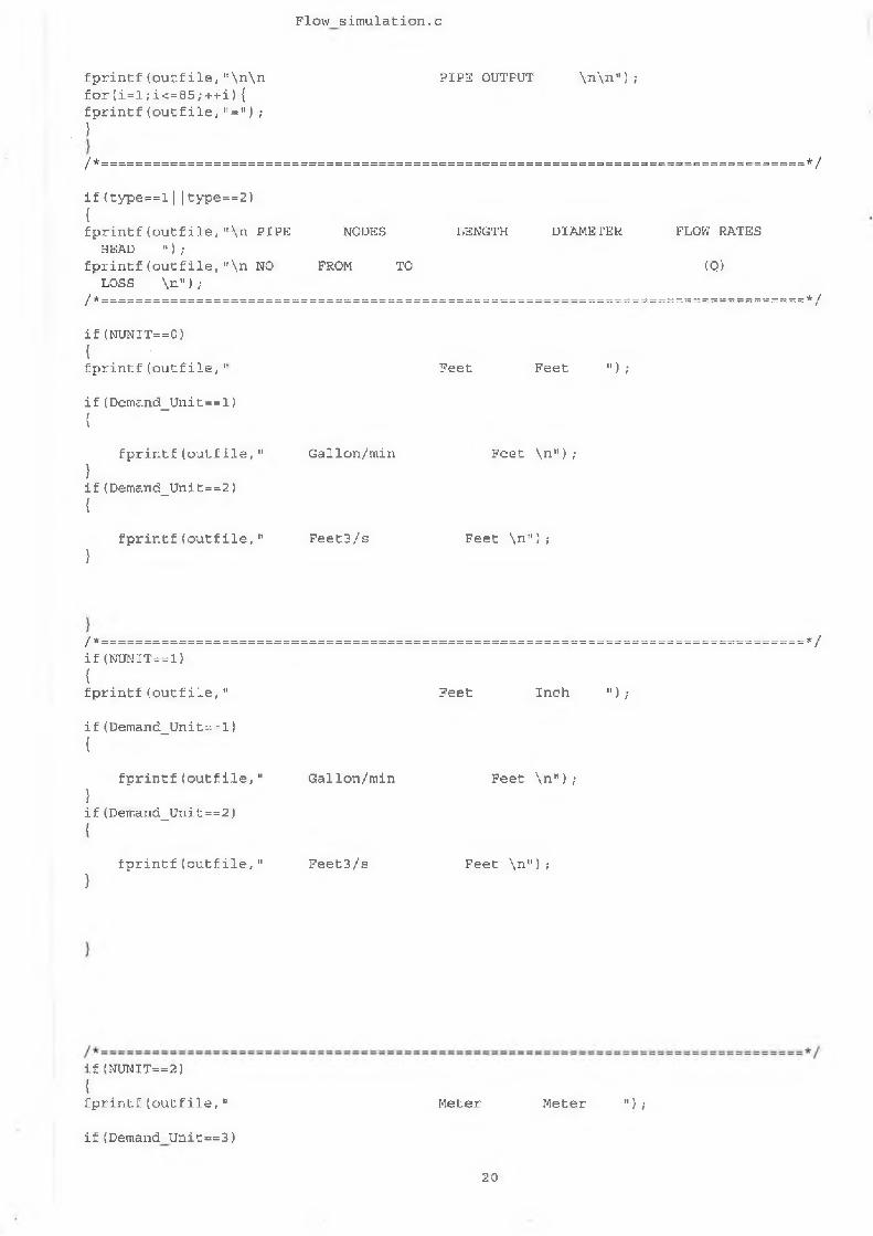
Flow simulation.c

f p r i n t f ( o u t f i l e , " \ n \ n P I P E O U T P U T \ n \ n " ) ;f o r ( i = l ; i < = 8 5 ; + + i ) { f p r i n t f ( o u t f i l e , " = " ) ;}

/ * = = = = = = = = = = = = = = = = = = = = = = = = = = = = = = = = = = = = = = = = = = = = = = = = = = = = = = = = = = = = = = = = = = = = = = = = = = = = = = = = = * /

i f ( t y p e = = l | | t y p e = = 2 ){f p r i n t f ( o u t f i l e , " \ n P I P E N O D E S L E N G T H D I A M E T E R F L O W R A T E S

H E A D " ) ;f p r i n t f ( o u t f i l e , " \ n N O F R O M T O ( Q )

L O S S \ n " ) ;/ * = = = , = = = = = = = = = = = = = = = = = = = = = = = = = = = = = = = = = = = = = = = = = = = = = = = = = = = = = = = = = = = = = = = = =* = = == = ==>= = = = = = * /

i f ( N U N I T = = 0 ){f p r i n t f ( o u t f i l e , " F e e t F e e t " ) ;

i f ( D e m a n d _ U n i t = = l ){

f p r i n t f ( o u t f i l e , " G a l l o n / m i n F e e t \ n " ) ;}i f ( D e m a n d _ U n i t = = 2 )I

f p r i n t f ( o u t f i l e , " F e e t 3 / s F e e t \ n " ) ;}

/ * = = = = = = = = = = = = = = = = = = = = = = = = = = = = = = = = = = = = = = = = = = = = = = = = = = = = = = = = = = = = = = = = = = = = = = = = = = = = = = = = = * /i f ( N U N I T = = 1 ){f p r i n t f ( o u t f i l e , " F e e t I n c h " ) ;

i f ( D e m a n d _ U n i t = = l )(

f p r i n t f ( o u t f i l e , " G a l l o n / m i n F e e t \ n " ) ;}i f ( D e m a n d _ U n i t = = 2 ){

f p r i n t f ( o u t f i l e , " F e e t 3 / s F e e t \ n " ) ;}

i f ( N U N I T = = 2 ){f p r i n t f ( o u t f i l e , " M e t e r M e t e r " ) ;

i f ( D e m a n d U n i t = = 3 )

20

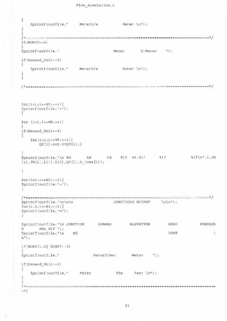
Flow simulation.c

f p r i n t f ( o u t f i l e , " M e t e r 3 / s M e t e r \ n " ) ;

/ * = = = = = = = = = = = = = = = I

i f ( N U N I T = = 3 ){f p r i n t f ( o u t f i l e , "

- * /

M e t e r C - M e t e r " ) ;

f p r i n t f ( o u t f i l e , " M e t e r 3 / s

i f ( D e m a n d _ U n i t = = 3 )f

}}

/ * -

M e t e r \ n " ) ;

f o r ( i = l ; i < = 8 5 ; + + i ) { f p r i n t f ( o u t f i l e , " = " ) ;)

f o r ( i = 1 ; i < = N P ; + + i ){i f ( D e m a n d _ U n i t = = l )i

f o r { i = l ; i < = N P ; + + i ) {Q F [ i ] = 4 4 9 . 0 * Q F [ i ] ; }

}f p r i n t f ( o u t f i l e , " \ n %d %d[ i ] , J B [ i ] , L [ i ] , D [ i ] , Q F [ i ] , h _ l o s s [ i ] )

%d % l f % 4 . 2 1 f % l f % l f \ n " , i , J A

}

f o r ( i = l ; i < = 8 5 ; + + i ) { f p r i n t f ( o u t f i l e , " = " ) ;}

/ * = = = = = = = = = = = = = = = = = = = = = = = = = = =f p r i n t f ( o u t f i l e , " \ n \ n \ n f o r ( i = l ; i < = 8 5 ; + + i ) { f p r i n t f ( o u t f i l e , " = " ) ;}

f p r i n t f ( o u t f i l e , " \ n J U N C T I O N E H G L E L V " ) ;f p r i n t f ( o u t f i l e \ n N O n " ) ;

i f ( N U N I T = = 2 I I N U N I T = = 3 ){f p r i n t f ( o u t f i l e , "

i f ( D e m a n d _ U n i t = = 3 ){

f p r i n t f ( o u t f i l e , " M e t e r}I/ * ==========================* /

J U N C T I O N S O U T P U T \ n \ n " ) ;

D E M A N D

M e t e r 3 / s e c

K P a

E L E V A T I O N

M e t e r ")

f e e t \ n " ) ;

H E A D

L O S S

P R E S S U R

\

21

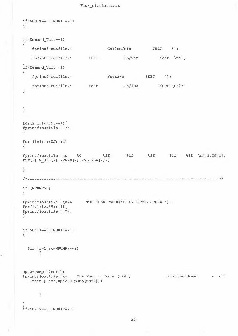
Flow simulation.c

i f ( N U N I T = = 0 | | N U N I T = = 1 )

{

i f ( D e m a n d _ U n i t = = l )

{f p r i n t f ( o u t f i l e , "

f p r i n t f ( o u t f i l e , "

}i f ( D e m a n d _ U n i t = = 2 )

{f p r i n t f ( o u t f i l e , "

f p r i n t f ( o u t f i l e , ”

}

}

f o r ( i = l ; i < = 8 5 ; + + i ) { f p r i n t f ( o u t f i l e , " = " ) ;}

f o r ( i = l ; i < = N J ; + + i ){

f p r i n t f ( o u t f i l e , " \ n %d % l f % l f % l f % l f % l f \ nE L T [ i ] , H _ J u n [ i ] , P R E S S [ i ] , H G L _ E L V [ i ] ) ;

/ * = = = = = = = = = = = = = = = = = = = = = = = = = = = = = = = = = = = = = = = = = = = = = = = = = = = = = = = = = = = = = = = = = = = = = = = = = =

i f ( N P U M P > 0 ){

f p r i n t f ( o u t f i l e , " \ n \ n T H E H E A D P R O D U C E D B Y P U M P S A R E \ n " ) ;f o r ( i = l ; i < = 8 5 ; + + i ) { f p r i n t f ( o u t f i l e , " = " ) ;}

i f ( N U N I T = = 0 | | N U N I T = = 1 )

{

f o r ( i = l ; i < = N P U M P ; + + i )

{

n p t 2 = p u m p _ l i n e [ i ] ;f p r i n t f ( o u t f i l e , " \ n T h e Pump i n P i p e [ %d ] p r o d u c e d Head

[ f e e t ] \ n " , n p t 2 , H _ p u m p [ n p t 2 ] ) ;

}

}i f ( N U N I T = = 2 | | N U N I T = = 3 )

G a l l o n / m i n F E E T » ) ;

F E E T L b / i n 2 f e e t \ n " ) ;

F e e t 3 / s F E E T •’ ) ;

F e e t L b / i n 2 f e e t \ n " ) ;

* /

= % l f

22

Flow simulation.c

{

f o r ( i = l ; i < = N P U M P ; + + i ) {

n p t 2 = p u m p _ l i n e [ i ] ;f p r i n t f ( o u t f i l e , " \ n T h e P u m p i n P i p e [ %d ] p r o d u c e d H e a d = % l f

[ m e t e r ] \ n " , n p t 2 , H _ p u m p [ n p t 2 ] ) ;

}

}

}f o r ( i = l ; i < = 8 5 ; + + i ) {

f p r i n t f ( o u t f i l e , " = " ) ;}

/*=================================================================================*/f o r ( i = l ; i < = N P ; + + i )i

i f ( N P V R > 0 ){

f o r ( j = l ; j < = N P V R ; + + j )i

i f ( Q F [ i ] = = Q J P V [ j ] ){

i f < Q F [ i ] > 0 ){

f p r i n t f ( o u t f i l e , " \ n \ n T H E P R V [ % d ] I N P I P E [ % d ] I S O P E R A T I N G N E O M A L LY \ n " , j , i ) ;

}

i f ( Q F [ i ] < 0 ){

f o r ( i = l ; i < = 8 5 ; + + i ) { f p r i n t f ( o u t f i l e , " = " ) ;}

f p r i n t f ( o u t f i l e , " \ n * * * * * * * * * * * * ( ( ( ( ( ( W A R N I N G ) ) ) ) ) ) * * * * * * * * * * * * * * * * \ n " ) ;f o r ( i = 1 ; i < = 8 5 ; + + i ) {

f p r i n t f ( o u t f i l e , " = " ) ;}

f p r i n t f ( o u t f i l e , " \ n \ n T H E P R V [ % d ] I N P I P E [ % d ] I S N O T O P E R A T I N G N E O M A L L Y \ n " , j , i ) ;

}

}}

}}

23

Flow simulation.c

}

{f p r i n t f ( o u t f i l e , " = " ) ;

}

f or(i = 1;i < = 8 5 ; + + i)

f c l o s e ( i n p u t _ f i l e ) ; f c l o s e ( o u t f i l e ) ;

} / * end o f m a i n f o r t h e f u n c t i o n o u t p u t () * /

/ * = = = = = = = = = = = = = = = = = = = = = = = = = = = = = = = = = = = = = = = = = = = = = = = = = = = = = = = = = = = = = = = = = = = = = = = = = = = = = = = = = * /

/ * = = = = = = = = = = = = = = = = = = = = = = = = = = = = = = = = = = = = = = = = = = = = = = = = = = = = = = = = = = = = = = = = = = = = = = = = = = = = = = * // * f u n c t i o n : L i n e a r _ D a r c y * // * I f t h e D a r c y - W e i s b a c h e q u a t i o n i s u s e d , t h i s f u n c t i o n w i l l b e c a l l e d * // * T h i s f u n c t i o n w i l l s e t up t h e m a s s c o n t i n u i t y , l o o p s e q u a t i o n s a s * // * a r r a y s , a n d c a l l i n g t h e G a u s s _ e l i m i n a t i o n s () t o s o l v e t h e s i m u l t a n e o u s * // * l i n e a r e q u a t i o n s . * // * T h i s f u n c t i o n c o m p u t e s t h e f l o w r a t e s o f e a c h p i p e i n t h e n e t w o r k b a s e d * // * on t h e u s e o f t h e D a r c y - W e i s b a c h e q u a t i o n f o r c o m p u t i n g t h e f r i c t i o n * // * l o s s . * // * * // * * // * = = = = = = = = = = = = = = = = = = = = = = = = = = = = = = = = = = = = = = = = = = = = = = = = = = = = = = = = = = = = = = = = = = = = = = = = = = = = = = * /

/*=================================================================================*/

i n t L i n e a r _ D a r c y ( d o u b l e Q J [ ] , d o u b l e Q F [ ] , i n t N P , i n t N J ,i n t N L , i n t J A [ ] , i n t J B [] , i n t N N J , i n t N N [ ] , i n t J N [ ] [MAX_SIZE] ,i n t NPVR, i n t I F L O W [ ] , i n t LP [] [ MA X_ SIZE ] , i n t L P L [ ] ,i n t N P S , i n t N L S J , i n t L P S L [ ] , i n t L P S [] [ MA X_S IZE ] ,d o u b l e A 0 [ ] , d o u b l e E L V [ ] , i n t N U N I T , i n t NoR,i n t NPUMP, i n t N L P U M , i n t LPUMSL [] , i n t LPUMS [] [ MAX^SIZE] ,d o u b l e H H O [ ] , d o u b l e h o [ ] , d o u b l e D [ ] , d o u b l e E [ ] , d o u b l e V I S ,d o u b l e e p s i l o n ,d o u b l e t o l , d o u b l e d e q , i n t m a x _ i t e r , d o u b l e K L L [ ] , i n t NP__PRV[], d o u b l e L [ ] , d o u b l e h ^ l o s s [ ] , d o u b l e H_pump [ ] , d o u b l e Q J P V [ ] , d o u b l e E L T [ ] , d o u b l e ENGY [ ] , d o u b l e s p g , d o u b l e H _ J u n [ ] , d o u b l e P RESS [ ] , i n t p u m p _ l i n e [ ] , d o u b l e H G L _ E L V [ ] )

/ * * /

i n t m a x _ e r = 1 0 0 ; i n t n u m l _ i t e r = 0 ; i n t num i t e r = 0 ;

24

Flow simulation.c

i n t t o l _ e x c e e d e d = T R U E ;i n t r e t 2 _ v a l , r e t u r n _ v a l u e , P R V F ;i n t i , j , I J , I I J , s s , R R , W W , r e s u l t , E E E , a s d a , n p t 2 ;i n t N X X , N E X T , N l , N 2 , N 3 , M B E G , M J J , m e m , J M A X , N T E P ;i n t k , J 8 , J 9 , J , J 1 , J 2 , J J , f f , N I P E , N U N , N U N O , K L , K J ;

i n t FF [ MAX_SIZE] , g g [ M A X _ S I Z E ] , EE [ MAX_SIZE] , a x a [ M A X _ S I Z E ] , n p t [ M A X _ S I Z E ] ;i n t J I J [ M A X _ S I Z E ] , J J U N [ M A X _ S I Z E ] , MPL [ M A X _ S I Z E ] , J X [ M A X _ S I Z E ] , f l a g p r v [ M A X _ S I Z E ]i n t M [ M A X _ S I Z E ] , N E X [ M A X ^ S I Z E ] , N I X [ M A X _ S I Z E ] , J P I P [ M A X _ S I Z E ] , J J I [ M A X _ S I Z E ] ;

double Re,e,f2,f1,BE,AE,EP,det,G2;

double Y[MAX_SIZE],YY[MAX_SIZE];double m[MAX_SIZE][MAX_SIZE],Q[MAX_SIZE],A[MAX_SIZE][MAX_SIZE];double ddd [MAX__SIZE] , DEQ [MAX_SIZE] ,Q1 [MAX_SIZE] , Q2 [MAX_SIZE] ;double QM1[MAX_SIZE],Q_old[MAX_SIZE],V[MAX_SIZE],V1[MAX_SIZE],V2[MAX_SIZE];double Rel[MAX_SIZE], Re2[MAX_SIZE];double EXPP[MAX_SIZE],KP[MAX_SIZE],AR[MAX_SIZE],ARL[MAX_SIZE]; double LL[MAX_SIZE],H_pump2[MAX_SIZE],QJPV2[MAX_SIZE];

for(i=l;i<=NP;++i){

if(NUNIT= = 0){

E[i]=E[i]/( 12 . 0*D [i] ) ;

)

if(NUNIT==1){

E[i]=E[i]/D[i] ;

D [i ] = D [i]/12.0 ;

}

if(NUNIT==2){

E[i]=E [i] *0.01/D [i] ;

)

if(NUNIT==3){

E[i]=E[i] /D[i] ;

D[i]=0.01*D [i] ;

)

}

if (NUNIT==0||NUNIT==1) {

25

Flow simulation.c

i f ( N U N I T = = 2 | | N U N T T = = 3 )

{G2 = 1 9 . 6 2 ;

}

G2 = 64 .4;

}

i f (NUNIT==0 || N U N I T = = 1 )

{f o r (i = 1 ; i < = N P ; + + i )

{

KP [ i ] = 0 . 00 0 9 3 5 1 7 * L [ i ] / p o w ( D [ i ] , 4 . 8 7 ) ;

A R [ i ] = 0 . 7 8 5 3 93 9 2 * p o w ( D [ i ] , 2 ) ;

ARL [ i ] = L [ i ] / (G2*D [ i ] * p o w ( A R [ i ] , 2) ) ;

)

}

i f (NUNIT==2I I N U N I T = = 3 )

{f o r ( i = l ; i < = N P ; + + i )

{

K P [ i ] = 0 . 0 0 2 1 2 * L [ i ] / p o w ( D [ i ] , 4 . 8 7 ) ;

A R [ i ] = 0 . 7 8 5 3 93 9 2 * p o w ( D [ i ] , 2 ) ;

ARL [ i ] = L [ i ] / ( G 2 * D [ i ] * p o w ( A R [ i ] , 2 ) ) ;

}

}

NUN=NP+NPUMP;

NUN0=NUN+1;

KL=NUN;

KJ=NUN;

/ * = === ======1= ======„ = = M========== ===== = === ===„ ============= ==s===-= = ==== = ===== ====* /

f o r ( i = l ; i < = K L ; + + i )

{f o r (j = 1 ; j < = K J ; + + j )

{A [ i ] [j ] = 0 . 0 ;

}}

26

Flow simulation.c

/ * ============================

i f ( N P U M P = = 0 & & N o R = = 0 ){

N J = N J - 1 ;}f o r ( i = l ; i < = N J ; + + i )

{

N N J = N N [ i ] ;

f o r ( j = l ; j < = N N J ; + + j ){

I J = J N [ i ] [ j ] ;I I J = a b s ( I J ) ; i f ( I J < 0 ){

A [ i ] [ I I J ] = - 1 . 0 ;

}

i f ( I J > 0 ){

A [ i ] [ I J ] = 1 . 0 ;

}

}}

/ * = = = = = = = = = = = = = = = = = = = = = = = = = = = = =

s s = l ;

f o r ( i = l ; i < = N J ; + + i ){

i f ( I F L O W [ i ] = = 0 ){

A [ i ] [ N U N O ] = 0 . 0 ;

}

e l s e

{

A [ i ] [ N U N O ] = Q J [ s s ] ;

SS=SS+1;}

*-

RR=NJ;

2 7

Flow simulation.c

f o r ( i = l ; i < = N L ; + + i ){

R R = 1 + R R ; N N J = L P L [ i ] ;

f o r ( j = l ; j < = N N J ; + + j ){

g g [ j ] = l p [ i ] [ j ] ;I I J = a b s ( g g [ j ] ) ; i f ( I I J < = N P )

{i f ( g g t j ] > o ){

A [RR] [ I I J ] =KP [ I I J ] ;

)i f ( g g [ j ] < 0 ){

A [ R R] [ I I J ] = - K P [ I I J ] ;

}A [ R R ] [ N U N O ] = 0 . 0 ;

}i f ( I I J > N P ) {

i f ( g g t j ] > o ){

A [ R R ] [ I I J ] = A O [ I I J ] ;A [ R R ] [ N U N O ] = - h o [ I I J ] ;

}i f ( g g [ j ] < o ){

A [RR] [ I I J ] = - A O [ I I J ] ;A [ R R ] [ N U N O ] = h o [ I I J ] ;

}

}

}

/ * -

f o r ( i = l ; i < = N P S ; + + i ){

R R = R R + 1 ;

N L S J = L P S L [ i ] ;

f o r ( j = 1 ; j < = N L S J ; + + j ){

F F [ j ] = L P S [ i ] [ j ] !

W W = a b s ( F F [ j ] ) ;

i f ( W W < = N P ){

i f ( F F [ j ] > 0 ){

A [ R R ] [WW] = K P [WW] ;

28

Flow simulation.c

}

i f ( F F [ j ] < 0 ){

A [ R R ] [ W W ] = - K P [ W W ] ;

}}

i f ( W W > N P ){

i f ( F F [ j ] > 0 ){

A [ R R ] [WW] = A O [WW] ;

}

i f ( F F [ j ] < 0 )i

A [ R R ] [WW] = - A O [WW] ;

}

}}

A [ R R ] [ N U N O ] = E L V [ i ] ;

)

/*=================================================================================*/

f o r ( i = l ; i < = N P U M P ; + + i ){

R R = R R + 1 ;N L P U M = L P U M S L [ i ] ; f o r ( j = 1 ; j < = N L P U M ; + + j ){

E E [ j ] = L P U M S [ i ] [ j ] ;E E E = a b s ( E E [ j ] ) ;

i f ( E E [ j ] < 0 )

{A [RR] [ E E E ] = - 1 . 0 ;

}

i f ( E E [ j ] > 0 )|

A [ R R ] [ E E E ] = 1 . 0 ;}

i f ( E E E > N P )[

A [RR] [ N U N O ] = H H O [ E E E ] ;

}

2 9

Flow simulation.c

/*=================================================================================*/

f o r ( i = l ; i < = N U N ; + + i ){

f o r ( j = l ; j < = N U N ; + + j ){

m [ i ] [ j ] = A [ i ] [ j ] ;

}

}

f o r ( i = l ; i < = N U N ; + + i ){

Q [ i ] = A [ i ] [ N U N O ] ;

)

r e s u l t = G a u s s e l i m i n a t i o n ( m , Q , N U N ( & d e t ) ;

i f ( r e s u l t = = 0 )1

/ / p r i n t f ( " \ n \ n \ t t h e s l u a t i o o f t h e s m u l a t i o n o f l i n e a r e q u a t i o n i s " ) ; / / p r i n t f ( " \ n t h e s l u a t i o n i s " ) ;

)

e l s e{

p r i n t f ( " \ n \ t * * * * * * * * W a r n i n g * * * * * * * * * * ») • p r i n t f ( " \ n \ n \ t T h e M a t r i x i s s i n g u l a r " ) ; s c a n f ( " % d " , & N P ) ;

}

f o r ( i = l ; i < = N U N ; + + i ){

Q _ o l d [ i ] = 0 . 0 ;}

w h i l e ( t o l _ e x c e e d e d £ c & n u m _ i t e r < m a x _ i t e r )

i f ( n u m _ i t e r = = 0 ){f o r ( i = l ; i < = N U N ; + + i ) {

30

HFlow simulation.c

Q 2 [ i ] = Q [ i ] ;Q l [ i ] = Q [ i ] ;Q 2 [ i ] = f a b s < Q 1 [ i ] ) ;

1i f ( n u m _ i t e r > 0 ){f o r ( i = l ; i < = N U N ; + + i ){

Q _ o l d [ i ] = Q 1 [ i ] ;Q M 1 [ i ] = 0 . 5 * ( Q 1 [ i ] + Q [ i ] ) ; Q l [ i ] = Q M l [ i ] ;Q 2 [ i ] = f a b s ( Q 1 [ i ] ) ;

}

}f o r ( i = 1 ; i < = N P ; + + i )

{

V [ i ] = ( Q 2 [ i ] ) / A R [ i l ;

D E Q [ i ] = Q 2 [ i ] * d e q ;

e = E [ i ] ;

d d d [ i ] = ( Q 2 [ i ] - D E Q [ i ] ) ;

V l [ i ] = ( Q 2 [ i ] - D E Q [ i ] ) / A R t i ] ;

R e l [ i ] = V 1 [ i ] * D [ i ] / V I S ;

R e = R e l [ i ] ;

r e t u r n _ v a l u e = N e w t o n _ R a p h s o n ( e p s i l o n , e , R e , m a x _ e r , & f 1 , & n u m l _ i t e r ) ;

V 2 [ i ] = ( Q 2 [ i ] + D E Q [ i ] ) / A R [ i ] ;

R e 2 [ i ] = V 2 [ i ] * D [ i ] / V I S ;R e = R e 2 [ i ] ;

r e t 2 _ v a l = N e w t o n _ R a p h s o n 2 ( f 1 , e p s i l o n , e , R e , m a x _ e r , & f 2 , & n u m l _ i t e r ) ;

s w i t c h ( r e t u r n _ v a l u e ){

c a s e 0 :/ / p r i n t f ( " f l = % 1 6 . 2 0 l e " , f l ) ; b r e a k ; c a s e 1 :

p r i n t f ( " \ n \ t * * * * * * * * W a r n i n g * * * * * * * * * * » ) ;p r i n t f ( " \ n t h e d e r i v a t i v e i s c l o s e t o z e r o " ) ; p r i n t f ( " \ n t h e c u r r e n t e s t i m a t e o f t h e f 1 = % 1 6 . 2 0 1 e " , f 1 ) ;

s c a n f ( " % d " , & N P ) ; c a s e 2 :

p r i n t f ( " \ n \ t * * * * * * * * W a r n i n g * * * * * * * * * * » ) ;p r i n t f ( " \ n \ n n e w t o n ' s m e t h o d d i d n o t c o n v e r g e " ) ; p r i n t f ( " \ n m a x i m u m n u m b e r o f i t e r a t i o n s e x c e e d e d " ) ; p r i n t f ( " \ n t h e c u r r e n t e s t i m a t e o f t h e f l = % 1 6 . 2 0 1 e " , f l ) ;

s c a n f ( " % d " , & N P ) ;

31

Flow simulation.c

s w i t c h ( r e t 2 _ v a l ){

c a s e 0 :/ / p r i n t f ( " f 2 = % 1 6 . 2 0 l e " , f 2 ) ;

b r e a k ; c a s e 1 :p r i n t f ( " \ n \ t * * * * * * * * W a r n i n g * * * * * * * * * * » ) ;p r i n t f ( " \ n n e w t o n ' s m e t h o d d i d n o t c o v e r a g e " ) ; p r i n t f ( " \ n t h e d e r i v a t i v e i s c l o s e t o z e r o " ) ; s c a n f ( " % d " , & N P ) ; b r e a k ; c a s e 2 :p r i n t f ( " \ n \ t * * * * * * * * W a r n i n g * * * * * * * * * * » ) ;p r i n t f ( " \ n m a x i m u m n u m b e r o f i t e r a t i o n s e x c e e d e d " ) ; p r i n t f ( " \ n t h e c u r r e n t e s t i m a t e o f t h e f 2 = % 1 6 . 2 0 l e " , f 2 ) ; s c a n f ( " % d " , & N P ) ;

}

B E = ( l o g l O ( f 1 ) - l o g l O ( f 2 ) ) / ( l o g l O ( Q 2 [ i ] + D E Q [ i ] ) - l o g l O ( Q 2 [ i ] - D E Q [ i ] ) ) ;A E = f l * p o w { ( Q 2 [ i ] - D E Q [ i ] ) , B E ) ;E P = 1 . 0 - B E ;E X P P t i ] = E P + 1 ;L L [ i ] = ( K L L [ i ] * p o w ( Q 2 [ i ] , 1 ) ) / ( G 2 * p o w ( A R [ i ] , 2 ) ) ;A R L [ i ] = L [ i ] * A E / ( G 2 * D [ i ] * p o w ( A R [ i ] , 2 ) ) ;K P [ i ] = ( A R L [ i ] ) * p o w ( Q 2 [ i ] , E P ) ;K P [ i ] = ( L L [ i ] + K P [ i ] ) ;

/ * = = = = = = = = = = = = = = = = = = = = = = = = = = = = = = = = = = = = = = = = = = = = = = = = = = = = = = = = = = = = = = = = = = = = = = = = = = = = = = = = = * /

}

R R = N J ; f o r ( i = l ; i < = N L ; + + i )

{R R = 1 + R R ;N N J = L P L [ i ] ;

f o r ( j = l ; j < = N N J ; + + j ){

g g [ j 1 = l p [ i ] [ j ] ;I I J = a b s ( g g [ j ] ) ;

i f ( I I J < = N P ){

i f ( g g [ j ] > o ){

A [R R ] [ I I J ] = K P [ I I J ] ;}

i f ( g g [ j ] < o ){

A [ R R ] [ I I J ] = - K P [ I I J ] ;}

A [ R R ] [ N U N O ] = 0 . 0 ;

}i f ( I I J > N P )

i f ( g g t j l > o )I

I

32

Flow simulation.c

A [ R R ] [ I I J ] = A 0 [ I I J ] * f a b s ( Q [ I I J ] ) ; A [ R R ] [ N U N O ] = - h o [ I I J ] ;

}i f (gg t j ] <o)i

A [ R R ] [ I I J ] = - A O [ I I J ] * f a b s ( Q [ I I J ] ) ; A [ R R ] [ N U N O ] = h o [ I I J ] ;

}

/ * = = = = = = = = = = = = = , = = - = = = = = = = = = = = = = = = = = = = = = = = = = = = = = = = = = = = = = = = = = = = = = = = = = = = = = = = = = = = = = = = = = * /

f o r ( i = l ; i < = N P S ; + + i ){

R R = R R + 1 ;

N L S J = L P S L [ i ] ;

f o r ( j = l ; j < = N L S J ; + + j ){

F F [ j ] = L P S [ i ] [ j ] ;

W W = a b s ( F F [ j ] ) ; i f ( W W < = N P )

{i f ( F F [ j ] > 0 ){

A [RR] [ W W ] = K P [ W W ] ;}

i f ( F F [ j ] < 0 ){

A [ R R ] [ W W ] = - K P [ W W ] ;}

}

i f ( W W > N P )i

i f ( F F [ j ] > 0 )i

A [ R R ] [ W W ] = A O [ W W ] * f a b s ( Q [ W W ] ) ;}

i f ( F F [ j ] < 0 ){

A[ RR] [ W W ] = - A O [ W W ] * f a b s ( Q [WW] ) ;

}

}

}

3 3

Flow simulation.c

/ * = = = = = = = = = = = = = = = = = = = = = = = = = = = = = = = = = = = = = = = = = = = = = = = = = = = = = = = = = = = = = = = = = = = = = = = = = = = = = = = = = = = =

f o r ( i = l ; i < = N U N ; + + i )

{f o r (j = l ; j < = N UN ; + + j )

{m [ i ] [ j ] = A [ i ] [ j ] ;

}

}f o r ( i = l ; i < = N U N ; + + i )

{Q [ i ] = A [ i ] [ N U N O ] ;

}

/ * = = = = = = = = = = = = = = = = = = = = = = = = = = = = = = = = = = = = = = = = = = = = = = = = = = = = = = = = = = = = = = = = = = = = = = = = = = = = = = = = = * /

r e s u l t = G a u s s _ e l i m i n a t i o n ( m , Q , N U N , & d e t ) ;

i f ( r e s u l t == 0)

{/ / p r i n t f ( " \ n \ n \ t t h e s l u a t i o o f t h e s m u l a t i o n o f l i n e a r e q u a t i o n i s " ) ;/ / p r i n t f ( " \ n t h e s l u a t i o n i s " ) ;

}

e l s e

{p r i n t f ( " \ n \ t * * * * * * * * W a r n i n g * * * * * * * * * * " ) ; p r i n t f ( " \ n \ n \ t t h e m a t r i x i s s i n g u l a r " ) ; s c a n f ( " % d " , & N P ) ;

}

/ * = = = = = = = = = = = = = = = = = = = = = = = = = = = = = = = = = = = = = = = = = = = = = = = = = = = = = = = = = = = = = = = = = = = = = = = = = = = = = = = = = * /

f o r ( i = l ; i < = N P ; + + i )

{Q F [ i ] = Q 1 [ i ] ;

}

/ * = = = = = = = = = = = = = = = = = = = = = = = = = = = = = = = = = = = = = = = = = = = = = = = = = = = = = = = = = = = = = = = = = = = = = = = = = = = = = = = = = * /f o r ( i = l ; i < = N P ; + + i )

{

h _ l o s s [ i ] = K P [ i ] * Q F ( i ] ;

}

f o r ( i = l ; i < = N U N ; + + i )

{

H _ p u m p [ i ] = 0 . 0 ;

}

i f (NPUMP>0)

{

3 4

Flow simulation.c

f o r ( i = l ; i < = N P U M P ; + + i )

{n p t [ i ] = p u m p _ l i n e [ i ] ; n p t 2 = a b s ( n p t [ i ] ) ;

f o r ( j = l ; j < = 2 ; + + j ){

a x a [ j ] = L P U M S [ i ] [ j ] ; a s d a = a b s ( a x a [ j ] ) ;

i f ( a s d a > N P )

{

H _ p u m p 2 [ n p t 2 ] = A 0 [ a s d a ] * Q 2 [ a s d a ] * Q 2 [ a s d a ] + h o [ a s d a ] ; H _ p u m p [ n p t 2 ] = H _ p u m p 2 [ n p t 2 ] ;

}}

}}

/ * =================================================================================* /

f o r ( i = l ; i < = N P ; + + i ){

i f ( N P V R > 0 ){

f o r ( j = l ; j < = N P V R ; + + j ){

f l a g p r v [ j ] = N P _ P R V [ j ] ;P R V F = a b s ( f l a g p r v [ j ] ) ;

i f ( P R V F = = i ){

Q J P V [ j ] = Q F [ i ] ; i f ( Q F t P R V F ] < = 0 ){

Q J P V 2 [ i ] = Q F [ i ] ;

Q J P V [ i ] = Q J P V 2 [ i ] ;

}

e l s e{

}}

}

}

3 5

Flow simulation.c

/ * =================

f o r ( i = l ; i < = N P ; + + i ){Y Y [ i ] = K P [ i ] * Q F [ i ] ; }

f o r ( 1 = 1 ; i < = N J ; + + i ){J X [ i ] = i ;}

}

N T E P = 0 ;f o r (j = 1 ; j < = N P ; + + j )

{N I P E = j ;J 1 = J A [ j ) ;J 2 = J B [ j ] ;i f ( ( J 1 + J 2 ) < = a b s ( J 1 - J 2 ) ) {

NT E P= NT EP +1 ; i f ( J A [ j ] >0)

{J J U N ( N T E P ) = J A [ j ] ;

}e l s e{

J J U N [ N T E P ] = J B [ j ] ;

}

J P I P [ N T E P ] = j ;

}}J J = 0 ;

f o r ( j = 1 ; j < = N J ; + + j ) {

i f ( J X [ j ] ! = 0 ){

J M A X = j ;J J = J J + 1 ;J J I [ J J ] = j ;

Flow simulation.c

N N J = N N [ i ] ;M [ 1 ] = 1 ;

i f ( i < = N J - l ){

M [ i + 1 ] = M ( i ] + N N J ;

}f o r ( j = l ; j < = N N J ; + + j ){

M P L t f f + 1 ] = J N [ i ] [ j ] ;

f f = f f + 1 ;

}

}

f o r ( i = l ; i < = N L ; + + i ){

N N J = L P L [ i ] ;f o r ( j = 1 ; j < = N N J ; + + j ){

M P L t f f + 1 ] = L P [ i ] [ j ] ;

f f = f f + 1 ;

}

}

f o r ( i = l ; i < = N J ; + + i ) {

Y [ i ] = 0 . 0 ;}N E X T = N T E P ;

f o r ( j = 1 ; j < = N E X T ; + + j ){

m e m = J JU N [ j ] ;

J 8 = J I J [ m e m ] ;

N E X [ j ] = J 8 ;

J 9 = J P I P t j ] ;

Y (J 8 ] = E N G Y [J 9 ] + Y Y [ J 9 ] - E L T [J 8 ] + H _ p u m p [ J 9 ] ; i f ( J A [ J 9 ] = = 0 )

{Y [J 8 ] = E N G Y [J 9 ] - Y Y [J 9 ] - E L T [J 8 ] + H _ p u m p [ J 9 ] ;

}}N X X = 0 ;

37

Flow simulation.c

f o r ( i = l ; i < = N J ; + + i ){M O :

i f < Y [ i ] = = 0 )I

f o r ( i = l ; i < = N E X T ; + + i )

{J = N E X [ i ] ;

M B E G = M [ J ] ; i f ( J < N J ){

M J J = M [ J + l ] - 1 ;

f o r ( k = M B E G ; k < = M J J ; + + k ){

N l = M P L [ k ] ;N l = a b s ( N l ) ;

N 2 = J A [ N 1 ] ;

N 3 = J B [ N l ] ;

i f ( N 2 = = J ){

i f ( N 3 = = 0 ){

c o n t i n u e ;}i f ( Y [ N 3 ] ! = 0 ){

c o n t i n u e ;}Y [ N 3 ] = Y [ N 2 ] - Y Y [ N l ] + H _ p u m p [ N l ] ;

N X X = N X X + 1 ;

N I X [ N X X ] = N 3 ;

i f ( N 2 = = 0 ){

c o n t i n u e ;}i f ( Y [ N 2 ] ! = 0 ){

c o n t i n u e ;

Y [ N 2 ] = Y [ N 3 ] + Y Y [ N l ] + H _ p u m p [ N l ] ;

N X X = N X X + 1 ;

N I X [ N X X ] = N 2 ;

}}}N E X T = N X X ;

Flow simulation.c

i f ( N E X T ! = 0 )I

f o r ( i = 1 ; i < = N E X T ; + + i ) {

N E X [ i ] = N I X [ i ] ;

}g o t o M O ;

} '

}}

f o r ( j = 1 ; j < = N J ; + + j )

{i f ( N U N I T = = 0 | | N U N I T = = 1 ){P R E S S [ j ] = ( Y [ j ] ) * s p g * 6 2 . 4 / 1 4 4 . 0 ; }i f ( N U N I T = = 2 | | N U N I T = = 3 ){P R E S S [ j ] = ( Y [ j ] ) * s p g * 9 . 8 0 7 ;}

)f o r ( j = 1 ; j < = N J ; + + j )

H G L _ E L V [ j ] = Y [ j ] + E L T [ j ] ;

}f o r ( j = l ; j < = N J ; + + j ) {

H _ J u n [ j ] = Y [ j ] ;

}

/ * = = = =

t o l _ e x c e e d e d = F A L S E ; f o r ( i = l ; i < = N P ; + + i ){i f ( f a b s ( Q 1 [ i ] - Q _ o l d [ i ] ) > f a b s ( Q _ o l d [ i ] * t o l ) ) t o l _ e x c e e d e d = T R U E ;|+ + n u m _ i t e r ;} / * - - - - - - - - - - - - - - - - - - - - - - - - - - - - - - - w h i l e - - - - - - - - - - - - - - - - - - - - - - - - - - - - * /r e t u r n ( t o l e x c e e d e d ) ;

Flow simulation.c

/ * = = = = = ^ = = = = = = = = = = = = = = = = = = = = = = = = = = = = = = = = = = = = = = = = = = = = = = = = = = = = = = = = = = = = = = = = = = = = = = = = = = = * /

/ * = = = = = = = = = = = = = = = = = = = = = = = = = = = = = = = = = = = = = = = = = = = = = = = = = = = = = = = = = = = = = = = = = = = = = = = = = = = = = = * /

/ * f u n c t i o n : L i n e a r _ H a z e n _ W i l l i a m * // * I f t h e H a z e n - W i l l i a m e q u a t i o n i s u s e d , t h i s f u n c t i o n w i l l b e c a l l e d * // * T h i s f u n c t i o n w i l l s e t up t h e ma s s c o n t i n u i t y , l o o p s e q u a t i o n s a s * // * a r r a y s , a n d c a l l i n g t h e G a u s s _ e l i m i n a t i o n s () t o s o l v e t h e s i m u l t a n e o u s * // * l i n e a r e q u a t i o n s . * // * T h i s f u n c t i o n c o m p u t e s t h e f l o w r a t e s o f e a c h p i p e i n t h e n e t w o r k b a s e d * // * on t h e u s e o f t h e H a z e n - W i l l i a m e q u a t i o n f o r c o m p u t i n g t h e f r i c t i o n * // * l o s s . * // * * // * * // * = = = = = = = = = = = = = = = = = = = = = = = = = = = = = = = = = = = = = = = = = = = = = = = = = = = = = = = = = = = = = = = = = = = = = = = = = = = = = = * /

/ * = = = = = = = = = = = = = = = = = = = = = = = = = = = = = = = = = = = = = = = = = = = = = = = = = = = = = = = = = = = = = = = = = = = = = = = = = = = = = = = = = * /

i n t L i n e a r _ H a z e n _ _ W i l l i a m s ( d o u b l e Q J [ ] , i n t N P , i n t N J ,i n t J A [ ] , i n t J B [] , i n t N L , i n t N N J , i n t NN[ ] , i n t J N [ ] [ MAX_SIZE] ,i n t NPVR, i n t I F L O W [ ] , i n t L P [ ] [ MA X_S IZE ] , i n t L P L [ ] ,i n t N P S , i n t N L S J , i n t L P S L [ ] , i n t L PS [] [ MA X_ SI ZE ] ,d o u b l e A O [ ] , d o u b l e E L V [ ] , i n t N U N I T , i n t NoR,i n t NPUMP, i n t N L P U M , i n t L P U M S L [] , i n t LPUMS [] [ M A X J 3 I Z E ] ,i n t NP _PR V[ ] , d o u b l e HHO[] , d o u b l e h o [ ] , d o u b l e CHW[] , d o u b l e K L L [ ] ,d o u b l e D [ ] , d o u b l e L [] , d o u b l e t o l , i n t m a x _ i t e r , d o u b l e h_ _ los s [] ,d o u b l e H_pump[] , d o u b l e Q J P V [ ] , d o u b l e E L T [ ] , d o u b l e ENGY[] ,d o u b l e s p g , d o u b l e H _ J u n [ ] , d o u b l e P R E S S [] )

{

i n t n u m _ i t e r = 0 ;i n t t o l _ e x c e e d e d = T R U E ;

i n t i , j , I J , I I J , s s , E E E , R R , r e s u l t , WW;i n t k , J 8 , J 9 , J , J 1 , J 2 , J J , f f , N I P E , N U N , N U N O , K L , K J , P R V F ; i n t g g [MAX_SIZE] , F F [ M A X _ S I Z E ] , E E [ M A X _ S I Z E ] ;i n t J I J [ M A X _ S I Z E ] , J J U N [ M A X _ S I Z E ] , MPL [M AX __ SI ZE] , J X [ M A X _ S I Z E ] , f l a g p r v [ M A X _ S I Z E ] ; i n t M [ M A X _ S I Z E ] , N E X [ M A X _ S I Z E ] , N I X [ M A X _ S I Z E ] , J P I P [ M A X _ S I Z E ] , J J I [ M A X _ S I Z E ] ; i n t NXX, N E XT , N 1 , N 2 , N 3 , MBEG, M J J , mem, J M A X , N T E P ;

d o u b l e d e t ;d o u b l e m [ M A X _ S I Z E ] [ M A X _ S I Z E ] , Q [ M A X _ S I Z E ] , A [ M A X _ S I Z E ] [ M A X _ S I Z E ] ; d o u b l e Q M 1 [ M A X _ S I Z E ] , Q _ o l d [ M A X _ S I Z E ] , Q 1 [ M A X _ S I Z E ] , Q 2 [ M A X _ S I Z E ] ; d o u b l e K P [M AX _ SI Z E] , DDL [MAX_SIZE] ; d o u b l e Y [ M A X _ S I Z E ] , Y Y [ M A X _ S I Z E ] ;

/ * = = = = = = = = = = = = = = = = = = = = = = = = = = = = = = = = = = = = = = = = = = = = = = = = = = = = = = = = = = = = = = = = = = = = = = = = = = = = = = = = = * /f o r ( i = l ; i < = N P ; + + i )

{i f ( N U N I T = = 1 )

{

D [ i ] = D [ i ] / l 2 . 0 ;

}

i f ( N U N I T = = 3 )

40

Flow simulation.c

)}

D[i]=0.01*D[i];

i f ( N U N I T = = 0 | | N U N I T = = 1 )(

f o r ( i = l ; i < = N P ; + + i ){

K P [ i ] = 4 , 7 3 * L [ i ] / ( p o w ( D [ i ] , 4 . 8 7 ) * p o w ( C H W [ i ] , 1 . 8 5 2 ) ) ;

}

}

i f ( N U N I T = = 2 | | N U N I T = = 3 )

{f o r ( i = l ; i < = N P ; + + i ){

K P [ i ] = 1 0 . 7 * L [ i ] / ( p o w ( D [ i ] , 4 . 8 7 ) * p o w ( C H W [ i ] , 1 . 8 5 2 ) ) ;

}

}

/ * = = = = = = = = = = = = = = = = = = = = = = = = = = = = = = = = = = = = = = = = = = = = = = = = = = = = = = = = = = = = = = = = = = = = = = = = = = = = = = = = = * /

N U N = N P + N P U M P ;

N U N 0 = N U N + 1 ;

K L = N U N ;

K J = N U N ;

f o r ( i = l ; i < = K L ; + + i ){

f o r ( j = l ; j < = K J ; + + j ) {A [ i ] [ j ] = 0 . 0 ;}

i f ( N P U M P = = 0 & & N o R = = 0 ) {

N J = N J - 1 ;}

/ * = = = = = = = = = = = = = = = = = = = = = = = = = = = = = = = = = = = = = = = = = = = = = = = = = = = = = = = = = = = = = = = = = = = = = = = = = = = = = = = = = * /

41

Flow simulation.c

f o r ( i = l ; i < = N J ; + + i )

{

N N J = N N [ i ] ;

f o r ( j = 1 ; j < = N N J ; + + j )

{

I J = J N [ i ] [ j ] ;

i f ( I J < 0 )

{I I J = a b s ( I J ) ; A [ i ] [ I I J ] = - 1 . 0 ;

}

i f ( I J > 0 )

{A [ i ] [ I J ] = 1 . 0 ;

}

}}

/ * = = = = = = = = = = = = = = = = = = = = ;

s s = l ;f o r ( i = l ; i < = N J ; + + i ){

i f ( I F L O W [ i ] = = 0 ){A [ i ] [ N U N O ] = 0 . 0 ;

}e l s e

{

A [ i ] [ N U N O ] = Q J [ s s ] ;

SS=SS+1;}

/ '

R R = N J ;f o r ( i = l ; i < = N L ; + + i )

{R R = 1 + R R ;

N N J = L P L [ i ] ;

f o r ( j = l ; j < = N N J ; + + j ){

g g [ j ] = L P [ i ] [ j ] ;

I I J = a b s ( g g [ j ] ) ;

i f ( I I J < = N P ){

42

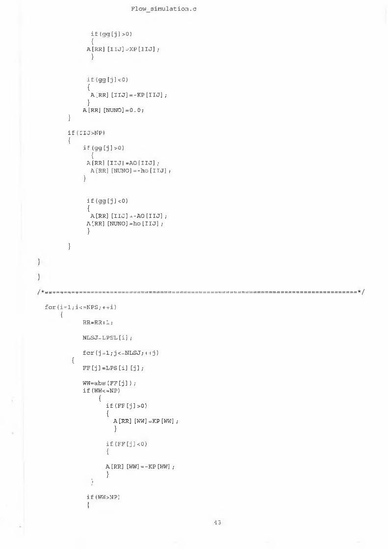
Flow simulation.c

i f < 9 9 [ j ] >0){

A [ R R ] [ I I J ] = K P [ I I J ] ;}

i f ( g g [ j ] < o ){A [ R R ] [ I I J ] = - K P [ I I J ] ;

}A [ R R ] [ N U N O ] = 0 . 0 ;

}

i f ( I I J > N P ){

i f ( g g ( j ) > o ){

A [ R R ] [ I I J ] = A O [ I I J ] ;A [ R R ] I N U N O ] = - h o [ I I J ] ;

}

i f ( g g [ j ] < 0 ){A[ RR] [ I I J ] = - A O [ I I J ] ;

A [ R R ] [ N U N O ] = h o [ I I J ] ;

}

}

/ * = = = = = = = = = = = = = = = = = = = = = = = = = = = = = = = = = = = = = = = = = = = = = = = = = = = = = = = = = = = = = = = = = = = = = = = = = = = = = = = = = * /

f o r ( i = l ; i < = N P S ; + + i )

{R R = R R + 1 ;

N L S J = L P S L [ i ] ;

f o r ( j = 1 ; j < = N L S J ; + + j ){

F F [ j ] = L P S [ i ] [ j ] ;

W W = a b s ( F F [j ] ) ; i f ( W W < =NP)

{i f ( F F [ j ] > 0 ){

A[ RR] [WW] =KP [WW] ;

}

i f ( F F [ j ] < 0 )i

A [RR] [WW] = - K P [WW] ;

}}

if(WW>NP)

{

43

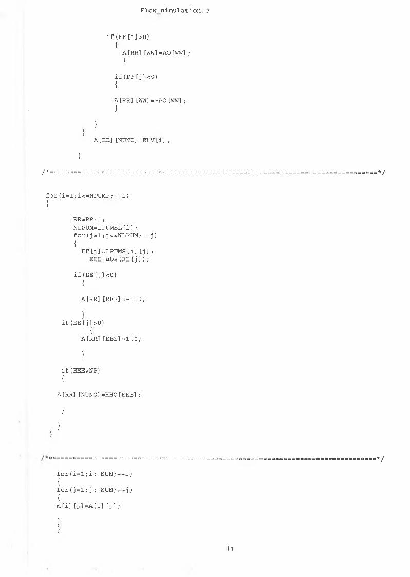
Flow simulation.c

i f ( F F [ j ] > 0 ){

A [ R R ] [WW] = A O [WW] ;}

i f ( F F [ j ] < 0 )

{

A [ R R ] [ W W ] = - A O [ W W ] ;}

}}

A [ R R ] [ N U N O ] = E L V [ i ] ;

}

/ * = = = = = = = = = = = = = = = = = = = = = = = = = = = = = = = = = = = = = = = = = = = = = = = = = = = = = = = = = = = = = = = = = = = = = = = = = = = = = = = = = * /

f o r ( i = l ; i < = N P U M P ; + + i ){

RR=RR+1 ;NLPUM=LPUMSL [ i ] ; f o r (j = 1 ; j <=NLPUM;+ + j )

{E E [ j ] =LPUMS [ i ] [ j ] ?

E E E = a b s ( E E [j ] ) ;

i f ( E E [ j ] <0)

{

A [ R R ] [ E E E ] = - 1 . 0 ;

}i f ( E E [ j ] >0)

{A [ R R ] [ E E E ] = 1 . 0 ;

}

i f ( E E E > N P )

{

A[ RR ] [NUNO] =HHO [EEE] ;

}

}}

f o r ( i = l ; i < =NUN; + + i )

{f o r (j = 1 ; j <=NUN; + + j )

{m [ i ] [j 1 = A [i] [ j ] ;

}}

* /

4 4

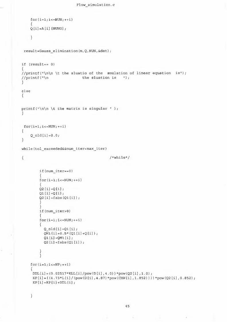
Flow simulation.c

f o r ( i = l ; i < = N U N ; + + i )

{Q t i ] = A [ i ] [NUNO] ;

}

r e s u l t = G a u s s e l i m i n a t i o n ( m , Q , N U N , & d e t ) ;

i f ( r e s u l t = = 0)

{/ / p r i n t f ( " \ n \ n \ t t h e s l u a t i o o f t h e s m u l a t i o n o f l i n e a r e q u a t i o n i s " ) ; / / p r i n t f ( " \ n t h e s l u a t i o n i s " ) ;

l s e

p r i n t f ( " \ n \ n \ t t h e m a t r i x i s s i n g u l a r " ) ;

f o r ( i = l ; i < = N U N ; + + i )

Q _ o l d [ i ] = 0 . 0 ;

w h i l e ( t o l _ e x c e e d e d & & n u m _ i t e r < m a x _ i t e r )

{ / * w h i l e * /

i f ( n u m _ i t e r = = 0 ){f o r ( i = l ; i < = N U N ; + + i ){Q 2 [ i ] = Q [ i ] ;Q l [ i ] = Q [ i ] ;Q 2 [ i ] = f a b s ( Q 1 [ i ] ) ;}}i f ( n u m _ i t e r > 0 ){f o r ( i = l ; i < = N U N ; + + i ){

Q _ o l d [ i ] = Q 1 [ i ] ;Q M 1 [ i ] = 0 . 5 * ( Q 1 [ i ] + Q [ i ] ) ;Q l [ i ] = Q M l [ i ] ;Q 2 [ i ] = f a b s ( Q 1 [ i ] ) ;

}}

f o r ( i = l ; i < = N P ; + + i ){

D D L [ i ] = ( 0 . 0 2 5 1 7 * K L L [ i ] / p o w ( D [ i ] , 4 . 0 ) ) * p o w ( Q 2 [ i ] , 1 . 0 ) ;K P [ i ] = ( ( 4 . 7 3 * L [ i ] / ( p o w ( D [ i ] , 4 . 8 7 ) * p o w ( C H W [ i ] , 1 . 8 5 2 ) ) ) ) * p o w ( Q 2 [ i ] , 0 . 8 5 2 ) ; KP t i ] = K P [ i ] + D D L [ i ] ;

}

45

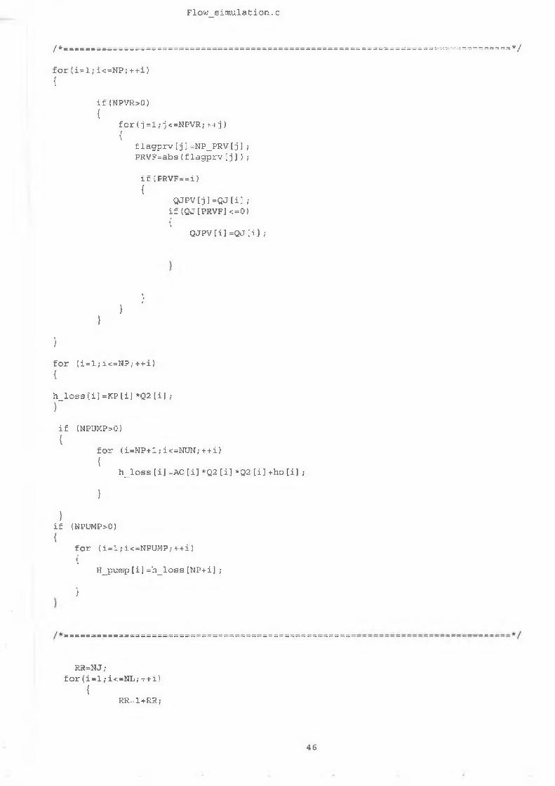
Flow simulation.c

/ * = = = = = = = = = = = = = = = = = = = = = = = = = = = = = = = = = = = = = = = = = = = = = = = = = = = = = = = = = = = = = = = = = = = = = = = = = = = = = = = = = * /

f o r ( i = l ; i < = N P ; + + i ){

i f ( N P V R > 0 ){

f o r ( j = 1 ; j < = N P V R ; + + j ){

f l a g p r v [ j ] = N P _ P R V [ j ] ;P R V F = a b s ( f l a g p r v [ j ] ) ;

i f ( P R V F = = i ){

Q J P V [ j ] = Q J [ i ] ; i f ( Q J [ P R V F ] < = 0 ){

Q J P V [ i ] = Q J [ i ] ;

}}

}

}

f o r ( i = l ; i < = N P ; + + i ){

h _ l o s s [ i ] = K P [ i ] * Q 2 [ i ] ;}

i f ( N P U M P > 0 )i

f o r ( i = N P + l ; i < = N U N ; + + i ){

h _ l o s s [ i ] = A 0 [ i ] * Q 2 [ i ] * Q 2 [ i ] + h o [ i ] ;

}

}i f ( N P U M P > 0 ){

f o r ( i = l ; i < = N P U M P ; + + i }t

H _ p u m p [ i ] = h _ l o s s [ N P + i ] j

}

R R = N J ; f o r ( i = l ; i < = N L ; + + i )

{R R = 1 + R R ;

4 6

Plow simulation.c

}

{

N N J = L P L [i] ;f o r ( j = 1 ; j < = N N J ; + + j ){

g g [ j ] = L P [ i ] [ j ] ; H J = a b s ( g g [ j ] ) ;

i f ( I I J < = N P )

i f ( g g [ j ] >0 ){

A [ R R ] [ I I J ] = K P [ I I J ] ; }

i f (ggtj] <0 ){A[ RR ] [ I I J ] = - K P [ I I J ] ;

}A[ RR ] [NUNO]= 0 . 0 ;

i f ( I I J > N P )

i f (gg [j]>o){

A [ R R ] [ I I J ] = A O [ I I J ] * f a b s ( Q [ I I J ] ) ; A [RR] [ N U N O ] = - h o [ I I J ] ;

}

i f ( g g [j ] <o){A [ R R ] [ I I J ] = - A O [ I I J ] * f a b s ( Q [ I I J ] ) ;

A [RR] [NUNO] = h o [ I I J ] ;

}

}* =/

f o r (i = l ; i < = N P S ; + + i )

{RR=RR+1;

N L S J = L P S L [ i ] ;

f o r ( j = l ; j < = N L S J ; + + j )

F F [ j ] = L P S [ i ] [ j ] ;

W W = a b s ( F F [ j ] ) ; i f ( W W < = N P )

{i f ( F F [ j ] > 0 ){

A [RR] [WW] = K P [WW] ;}

4 7

Flow simulation.c

i f ( F F [ j ] < 0 ){

A [ R R ] [ W W ] = - K P [ W W ] ;}

}

i f ( W W > N P ){

i f ( F F [ j ] > 0 ){

A [ R R ] [ W W ] = A O [ W W ] * f a b s ( Q [ W W ] ) ; }

i f ( F F [ j ] < 0 ){

A [ R R ] [ W W ] = - A O [ W W ] * f a b s ( Q [ W W ] ) ;}

}}

}

/ * = = = = = = = = = = = = = = = = = = = = = = = = = = = = = = = = = = = = = = = = = = = = = = = = = = = = = = = = = = = = = = = = = = = = = = = = = = = = = = = = = * /

f o r ( i = l ; i < = N U N ; + + i ){

f o r ( j = l ; j < = N U N ; + + j ){

m [ i ] [ j ] = A [ i ] [ j ] ;

}

}f o r ( i = l ; i < = N U N ; + + i )

{Q [ i ] = A [ i ] [ N U N O ] ;

}

r e s u l t = G a u s s e l i m i n a t i o n ( m , Q , N U N , & d e t ) ;

i f ( r e s u l t = = 0 ){/ / p r i n t f ( " \ n \ n \ t t h e s l u a t i o o f t h e s m u l a t i o n o f l i n e a r e q u a t i o n i s " ) ; / / p r i n t f ( " \ n t h e s l u a t i o n i s " ) ;}

e l s ei

p r i n t f ( " \ n \ n \ t * * * * * * W a r n i n g * * * * * * * * » ) ;p r i n t f ( " \ n \ n \ t T h e m a t r i x i s s i n g u l a r " ) ; s c a n f { " % d " ( & N P ) ;}

4 8

Flow simulation.c

f o r ( i = l ; i < = N P ; + + i )

Q J [ i ] = Q l [ i ] ;}

/ * = = = = = = = = = = = = = = = = = = = = = = = = = = = = = = = = = = = = = = = = = = = = = = = = = = = = = = = = = = = = = = = = = = = = = = = = = = = = = = = = = * /

f o r ( i = l ; i < = N P ; + + i ){Y Y [ i ] = K P [ i ] * Q [ i ] ;}

f o r ( i = l ; i < = N J ; + + i ){J X [ i ] = i ;}

{

N T E P = 0 ;f o r ( j = l ; j < = N P ; + + j )

{N I P E = j ;J 1 = J A [ j ] ;J 2 = J B [ j ] ;i f ( ( J 1 + J 2 ) < = a b s ( J 1 - J 2 ) )

{N T E P = N T E P + 1 ; i f ( J A t j ] > 0 )

{J J U N [ N T E P ] = J A [ j ] ;

}e l s e{

J J U N [ N T E P ] = J B [ j ] ;

}

J P I P [ N T E P ] = j ;

}}J J = 0 ;

f o r { j = 1 ; j < = N J ; + + j ) {

i f ( J X [ j ] ! = 0 ){

J M A X = j ;J J = J J + 1 ;J J I [ J J ] = j ;J I J t j ] = J J ;

}}

f f = 0 ;f o r ( i = l ; i < = N J ; + + i )

4 9

Flow simulation.c

N N J = N N [ i ] ;M [ 1 ] = 1 ;

i f ( i < = N J - 1 ){

M [ i + 1 ] = M [ i ] + N N J ;

}f o r ( j = l ; j < = N N J ; + + j )<

M P L [ f f + 1 ] = J N [ i ] [ j ] ;

{

f f = f f + 1 ;

}

}

f o r ( i = l ; i < = N L ; + + i ){

N N J = L P L [ i ] ;f o r { j = 1 ; j < = N N J ; + + j ) {

M P L t f f + 1 ] = L P [ i ] [ j ] ;

f f = f f + 1 ;

}

/ * = = = = = = = = = = = = = = = = = = = = = = = = = = = = = = = = = = = = = = = = = = = = = = = = = = = = = = = = = = = = = = = = = = = = = = = = = = = = = = = = = * /

f o r ( i = l ; i < = N J ; + + i ){

Y [ i ] = 0 . 0 ;}N E X T = N T E P ;

f o r ( j = l ; j < = N E X T ; + + j ){

m e m = J J U N [ j ] ;

J 8 = J I J [ m e m ] ;

N E X [ j ] = J 8 ;

J 9 = J P I P [ j ] ;

Y [ J 8 ] = E N G Y [ J 9 ] + Y Y [ J 9 ] ;

i f ( J A [ J 9 ] = = 0 ){

50

Flow simulation.c

Y [ J 8 ] = E N G Y [ J 9 ] - Y Y [ J 9 ] ;

}N X X = 0 ;f o r ( i = l ; i < = N J ; + + i ){M O :

i f ( Y [ i j = = 0 ){

}

f o r ( i = l ; i < = N E X T ; + + i )

{J = N E X [ i ] ;

MBEG=M[J ] ; i f ( J < N J )

{

MJJ=M [ J + l ] - 1 ;

f o r ( k = M B E G ; k < = M J J ; + + k )

{

N 1 = M P L [ k ] ;N l = a b s ( N l ) ;

N 2 = J A [ N 1 ] ;

N 3 = J B [ N l ] ;

i f ( N 2 = = J )

{i f ( N 3 = = 0 ){

c o n t i n u e ;

)i f (Y [N3] ! =0)

{c o n t i n u e ;

}Y [ N 3 ] = Y [ N 2 ] - Y Y [ N l ] ;

NXX= NXX+1 ;

N I X [ N X X ] = N 3 ;

}i f ( N 2 = = 0 )

{c o n t i n u e ;

}i f ( Y [ N 2 ] ! = 0 )

{c o n t i n u e ;

Y [ N 2 ] = Y [ N 3 ] + Y Y [ N 1 ] ;

N X X = N X X + 1 ;

51

Flow simulation.c

N I X [ N X X ] = N 2 ;

}}

}N E X T = N X X ;

i f ( N E X T ! = 0 ) {

f o r ( i = l ; i < = N B X T ; + + i ) {

N E X [ i ] = N I X [ i ] ;

g o t o M O ; } '

}}

f o r ( j = 1 ; j < = N J ; + + j )

{i f [ N U N I T = = 0 | | N U N I T = = 1 ){P R E S S [ j ] = < Y [ j ] - E L T [ j ] ) * s p g * 6 2 . 4 / 1 4 4 . 0 ; }i f ( N U N I T = = 2 | | N U N I T = = 3 ){P R E S S [ j ] = ( Y [ j ] - E L T [ j ] ) * s p g * 9 . 8 0 7 ;}

f o r ( j = l ; j < = N J ; + + j ){

H _ J u n [ j ] = Y [ j ] ;

}

t o l _ e x c e e d e d = F A L S E ; f o r ( i = l ; i < = N P ; + + i )

{i f ( f a b s ( Q 1 [ i ] - Q _ o l d [ i ] ) > f a b s ( Q _ o l d [ i ] * t o l ) ) t o l _ e x c e e d e d = T R U E ;

}+ + n u m _ i t e r ;} / * ---------------------------------------w h i l er e t u r n ( t o l e x c e e d e d ) ;

52

Flow simulation.c

/ * = = = = = = = = = = = = = = = = = = = = = = = = = = = = = = = = = = = = = = = = = = = = = = = = . = = = = = = = = = = = = = = = = = = = = = = = = = = = = = = = = = = * // * f u n c t i o n : G a u s s _ e l i m i n a t i o n * // * t h i s f u n c t i o n s o l v e s t h e s y s t e m o f e q u a t i o n s [ A ] {x}={B} u s i n g t h e * // * G a u s s e l i m i n a t i o n m e t h o d w i t h p a r t i a l p i v o t i n g . * // * * /

/ * = = = = = = = = = = = = = = = = = = = = = = = = = = = = = = = = = = = = = = = = = = = = = = = = = = = = = = = = = = = = = = = = = = = = = = = = = = = = = = = = = * /

i n t G a u s s _ e l i m i n a t i o n ( d o u b l e a [ ] [ M A X _ S I Z E ] , d o u b l e b [ ] , i n t n , d o u b l e * p t r _ d e t )

d o u b l e t e m p , m u l t , t r t , t o l ; i n t n p i v o t , i , j , k , 1 , e r r o r _ f l a g ;

* p t r _ d e t = l . 0 ; t o l = l e - 3 0 ; n p i v o t = l ;

f o r ( k = l ; k < = n - l ; + + k ) {

f o r ( i = k ; i < = n , - + + i ) {

i f ( f a b s ( a [ i ] [ k ] ) > f a b s ( a [ k ] [ k ] ) ) {

+ + n p i v o t ;f o r ( l = l ; l < = n ; + + l ){

t e m p = a [ i ] [ 1 ] ; a [ i ] [ 1 ] = a [ k ] [ 1 ] ; a [ k ] [ 1 ] = t e m p ;

}

t e m p = b [ i ] ; b [ i ] = b [ k ] ; b [ k ] = t e m p ;

}

}

t r t = * p t r _ d e t ;

t r t = * p t r _ d e t * a [ k ] [ k ] ; i f ( f a b s ( t r t ) < t o l )

{e r r o r _ f l a g = l ;

53

Flow simulation.c f

r e t u r n ( e r r o r _ f l a g ) ;

}

f o r ( i = 2 ; i < = n ; + + i )

{i f ( i ! = k )

{m u l t = a [ i ] [ k ] / a [ k ] [k] ;

b [ i ] = b [ i ] - b [ k ] * m u l t ;

f o r (j = 1 ; j < = n ; + + j )

{a [ i ] [ j 3 —a [ i ] [ j ] - a [k] t j ] * m u l t ;

}}

}

i f ( n p i v o t % 2 = = 1 )* p t r _ d e t = * p t r _ d e t * ( - 1 . 0 ) ;

/ * = = = = = = = = = = = = = = = = = = = = = = = = = = = = = = = = = = = = = = = = = = = = = = = = = = = = = = = = = = = = = = = = = = = = = = = = = = = = = = = = = : * /

b [ n ] = b [ n ] / a [n] [ n ] ;

f o r ( i = n - l ; i > = l ; i - - ){

f o r ( j = i + l ; j < = n ; + + j )

b [ i ] = b [ i ] - a [ i ] [ j ] * b [ j ] ; b [ i ) = b [ i ] / a [ i ] C i ] ;

e r r o r _ f l a g = 0 ; r e t u r n ( e r r o r _ f l a g ) ;

/ * = = = = = = = = = = = = = = = = = = = = = = = = = = = = = = = = = = = = = = = = = = = = = = = = = = = = = = = = = = = = = = = = = = = = = = = = = = = = = * /

/ * = = = = = = = = = = = = = = = = = = = = = = = = = = = = = = , --------= = = = = = = = = = = = = = = = = = = = = = = = = = = = = = = = = = = = = = = = = = = * // * f u n c t i o n : N e w t o n - R a p h s o n ( ) * // * t h i s f u n c t i o n c o m p u t e s t h e r o o t o f an e q u a t i o n o f t h e f o r m F ( x ) = 0 * // * u s i n g t h e N e w t o n - R a p h s o n m e h t o d , i . e . c o m p u t e s t h e v a l u e o f t h e f r i c t i o n * // * f a c t o r f . * /

/ * * // * = = = = = = = = = = = = = = = = = = = = = = = = = = = = = = = = = = = = = = = = = = = = = = = = = = = = = = = = = = = = = = = = = = = = = = = = = = = = = * /

/ * = = = = = = = = = = = = „ = = = = = = = = = = = = = = = = = = = = = = = = = = = = = = = = = = = = = = = = = = = = = = = = = = = = = = = = = = = = = = * /

i n t N e w t o n _ R a p h s o n ( d o u b l e e p s i l o n . d o u b l e e , d o u b l e Re,

54

Flow simulation.c

i n t m a x _ e r , d o u b l e * p t r _ f l , i n t * p t r _ n u m l _ i t e r )

d o u b l e x _ p r e v ; d o u b l e x _ c u r r ; d o u b l e d e r f ;* p t r _ n u m l _ i t e r = 0 ;x _ p r e v = l . 0 / p o w { 1 . 1 4 - 2 . 0 * l o g l 0 ( e ) , 2 ) ; x _ c u r r = l . 0 / p o w ( l . 1 4 - 2 . 0 * l o g l 0 ( e ) , 2 ) ;

w h i l e ( * p t r _ n u m l _ i t e r < m a x _ e r ){

d e r f = d f ( x _ p r e v , e , R e ) ;i f ( f a b s ( d f ( x _ p r e v , e , R e ) ) < = n e a r l y _ z e r o ) r e t u r n ( 1 ) ;x _ c u r r = x _ p r e v - f ( x _ p r e v , e , R e ) / d e r f ;+ + * p t r _ n u m l _ i t e r ;* p t r _ f l = x _ c u r r ;i f ( f a b s ( x _ c u r r - x _ p r e v ) < = f a b s ( x _ c u r r * e p s i l o n ) ) r e t u r n ( 0 ) ; x _ p r e v = x _ c u r r ;

}

{

r e t u r n ( 2 ) ;}/ * = = = = = = = = = = = = = = = = = = = = = = = = = = = = = = = = = = = = = = = = = = = = = = = = = = = = = = = = = = = = = = = = = = = = = = = = = = = = = = = = = * /

/ * =============== = ============================================= = * /

/ * f u n c t i o n : f ( ) * // * p u r p o s e : c o m p u t e t h e v a l u e o f f [ x ] a t x * // * * // * = = = = = = = = = = = = = = = = = = = = = = = = = = = = = = = = = = = = = = = = = = = = = = = = = = = = = = = = = = = = = = = = = = = = = = = = = = = = = = = = = * /

d o u b l e f ( d o u b l e x , d o u b l e e , d o u b l e R e ){

d o u b l e f x ;

f x = l . / ( s q r t ( x ) ) - 1 . 1 4 + 2 . * l o g l 0 ( ( e ) + 9 . 3 5 / ( R e * s q r t ( x ) ) ) ; r e t u r n ( f x ) ;}

/ * = = = = = = = = = = = = = = = = = = = = = = = = = = = = = = = = = = = = = = = = = = = = = = = = = = = = = = = = = = = = = = = = = = = = ............ = = = = = = = = * /

/ * f u n c t i o n : d f ( ) * // * p u r p o s e : c o m p u t e t h e v a l u e o f d f [ x ] a t x * // * * // * = = = = = = = = = = = = = = = = = = = = = = = = = = = = = = = = = = = = = = = = = = = = = = = = = = = = = = = = = = = = = = = = = = = = = = = = = = = = = = = = = * /

d o u b l e d f ( d o u b l e x , d o u b l e e , d o u b l e R e ) {d o u b l e d f x ;

d o u b l e A R G ; d o u b l e M O R ; d o u b l e D A R ;

5 5

Flow simulation.c

A R G = 9 . 3 5 * l o g l 0 ( 2 . 7 1 8 2 8 ) ;MOR=( ( e ) + 9 . 3 5 / ( R e * s q r t ( x ) ) ) ; D A R = x * s q r t ( x ) * R e ;

d f x = - 0 . 5 / ( x * s q r t ( x ) ) - ( ARG/ (DAR*MOR) ) ; r e t u r n ( d f x ) ;

}

/ * = = = = = = = = = = = = = = = = = = = = = = = = = = = = = = = = = = = = = = = = = = = = = = = = = = = = = = = = = = = = = = = = = = = = = = = = = = = = = = = = == * // * f u n c t i o n : P o l y _ l e a s t s q r

* // * p u r p o s e : i f a pump e x i s t i n t h e n e t w o r k , a n d i t s c h a r a c t e r i s t i c i s d e s c r i b e d b y

* // * p e r f o r m a n c e o p e r a t i n g d a t a . T h i s f u n c t i o n i n v o k e d t o f i t t h e c u r v e f o r t h e

* // * d a t a u s i n g l e a s t s q u a r e m e t ho d

* /

/ * = = = = = = = = = = = = = = = = = = = = = = = = = = = = = = = = = = = = = = = = = = = = = = = = = = = = = = = = = = = = = = = = = = = = = = = = = = = = = = = = =

i n t p o l y _ l e a s t s q r ( d o u b l e x [ ] , d o u b l e y [ ] , i n t n u m _ p o i n t s , i n t n u m _ p o l y , d o u b l e a o [ ] )

{d o u b l e c [ M A X _ S I Z E ] [ M A X _ S I Z E ] •d o u b l e s [ 2 * M A X _ S I Z E ] ;i n t i , j ;d o u b l e d e t ;i n t r e s u l t ;s [ 0 ] = n u m _ p o i n t s ;f o r ( i = l ; i < = 2 * n u m _ p o l y ; + + i )

{S [ i ] = 0 . 0 ;f o r (j = 1 ; j < = n u m _ p o i n t s ; + + j ) s [ i ] + = p o w ( x [ j ] , i ) ;

for(i=0;i<=num_poly;++i) for(j =0 ;j <=num_poly;++j)C [i + 1] [j+1] =S [i+j] ;ao [1]=0.0;for(j =1;j<=num_points;++j) ao [1] +=y [j ] ;for(i=l;i<=num_poly;++i){ao [i + 1]=0.0 ;for(j =1;j <=num_points;++j) ao [i+1] +=y [j ] *pow(x [j ] , i) ;}

r e s u l t = G a u s s _ e l i m i n a t i o n ( c , a o , n u m _ p o l y + l , & d e t ) ; r e t u r n ( r e s u i t ) ;

/ * = = = = = = = = = = = = = = = = = = = = = = = = = = = = = = = = = = = = = = = = = = = = = = = = = = = = = = = = = = = = = = = = = = = = = = = = = = = = = = = = = * /

/ * = = = = = = = = = = = = = = = = = = = = = = = = = = = = = = = = = = = = = = = = = = = = = = = = = = = = = = = = = = = = = = = = = = = = = = = = = = = = = = = = = * /

56

Flow simulation.c

i n t N e w t o n _ R a p h s o n 2 ( d o u b l e f l , d o u b l e e p s i l o n , d o u b l e e , d o u b l e R e , i n t m a x _ e r , d o u b l e * p t r _ f 2 , i n t * p t r _ n u m l _ i t e r )

d o u b l e x _ p r e v ; d o u b l e x _ c u r r ;

d o u b l e d e r f ;

* p t r _ n u m l _ i t e r = 0 ; x _ p r e v = f l ; x _ c u r r = f l ;

w h i l e ( * p t r _ n u m l _ i t e r < m a x _ e r ){

d e r f = d f ( x _ p r e v , e , R e ) ;i f ( f a b s ( d f ( x _ p r e v , e , R e ) ) < = n e a r l y _ z e r o ) r e t u r n ( 1 ) ;x _ c u r r = x _ p r e v - f ( x _ p r e v , e , R e ) / d e r f ;

+ + * p t r _ n u m l _ i t e r ;* p t r _ f 2 = x _ c u r r ;i f ( f a b s ( x _ c u r r - x _ p r e v ) < = f a b s ( x _ c u r r * e p s i l o n ) ) r e t u r n ( 0 ) ; x _ p r e v = x _ c u r r ;

i

r e t u r n ( 2 ) ;}

{

5 7