Embed Size (px)
Citation preview
MODELING AND SIMULATION OF THE FLUID FLOW IN ARTIFICIALLY
FRACTURED AND GEL TREATED CORE PLUGS
A THESIS SUBMITTED TO
THE GRADUATE SCHOOL OF NATURAL AND APPLIED SCIENCES
OF
MIDDLE EAST TECHNICAL UNIVERSITY
BY
ONUR ALP KAYA
IN PARTIAL FULFILLMENT OF THE REQUIREMENTS
FOR
THE DEGREE OF MASTER OF SCIENCE
IN
PETROLEUM AND NATURAL GAS ENGINEERING
SEPTEMBER 2021

Approval of the thesis:
MODELING AND SIMULATION OF THE FLUID FLOW IN
ARTIFICIALLY FRACTURED AND GEL TREATED CORE PLUGS
submitted by NAME SURNAME in partial fulfillment of the requirements for the
degree of Master of Science in Petroleum and Natural Gas Engineering, Middle
East Technical University by,
Prof. Dr. Halil Kalıpçılar
Dean, Graduate School of Natural and Applied Sciences
Assoc. Dr. Çağlar Sınayuç
Head of the Department, Petroleum and Natural Gas Eng.
Assist. Prof. Dr. İsmail Durgut
Supervisor, Petroleum and Natural Gas Eng., METU
Examining Committee Members:
Prof. Dr. Mahmut Parlaktuna
Petroleum and Natural Gas Eng., METU
Assist. Prof. Dr. İsmail Durgut
Petroleum and Natural Gas Eng., METU
Assist. Prof. Dr. Doruk Alp
Petroleum and Natural Gas Eng., METU NCC
Date: 09.03.2021

iv
I hereby declare that all information in this document has been obtained and
presented in accordance with academic rules and ethical conduct. I also declare
that, as required by these rules and conduct, I have fully cited and referenced
all material and results that are not original to this work.
Name Last name :
Signature :
v
ABSTRACT
MODELING AND SIMULATION OF THE FLUID FLOW IN
ARTIFICIALLY FRACTURED AND GEL TREATED CORE PLUGS
Kaya, Onur Alp
Master of Science, Petroleum and Natural Gas Engineering
Supervisor : Asst.Prof. Dr. İsmail Durgut
September 2021, 137 pages
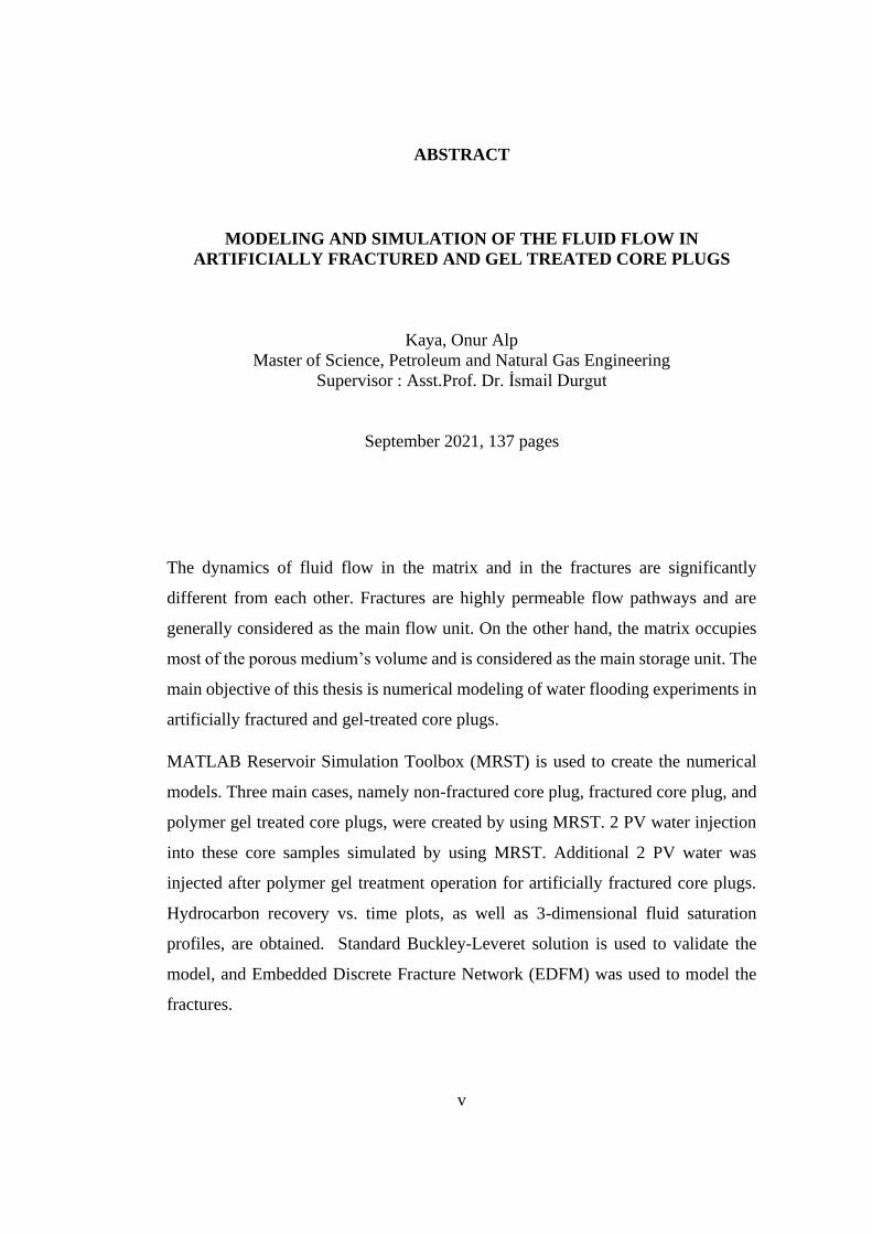
The dynamics of fluid flow in the matrix and in the fractures are significantly
different from each other. Fractures are highly permeable flow pathways and are
generally considered as the main flow unit. On the other hand, the matrix occupies
most of the porous medium’s volume and is considered as the main storage unit. The
main objective of this thesis is numerical modeling of water flooding experiments in
artificially fractured and gel-treated core plugs.
MATLAB Reservoir Simulation Toolbox (MRST) is used to create the numerical
models. Three main cases, namely non-fractured core plug, fractured core plug, and
polymer gel treated core plugs, were created by using MRST. 2 PV water injection
into these core samples simulated by using MRST. Additional 2 PV water was
injected after polymer gel treatment operation for artificially fractured core plugs.
Hydrocarbon recovery vs. time plots, as well as 3-dimensional fluid saturation
profiles, are obtained. Standard Buckley-Leveret solution is used to validate the
model, and Embedded Discrete Fracture Network (EDFM) was used to model the
fractures.
vi
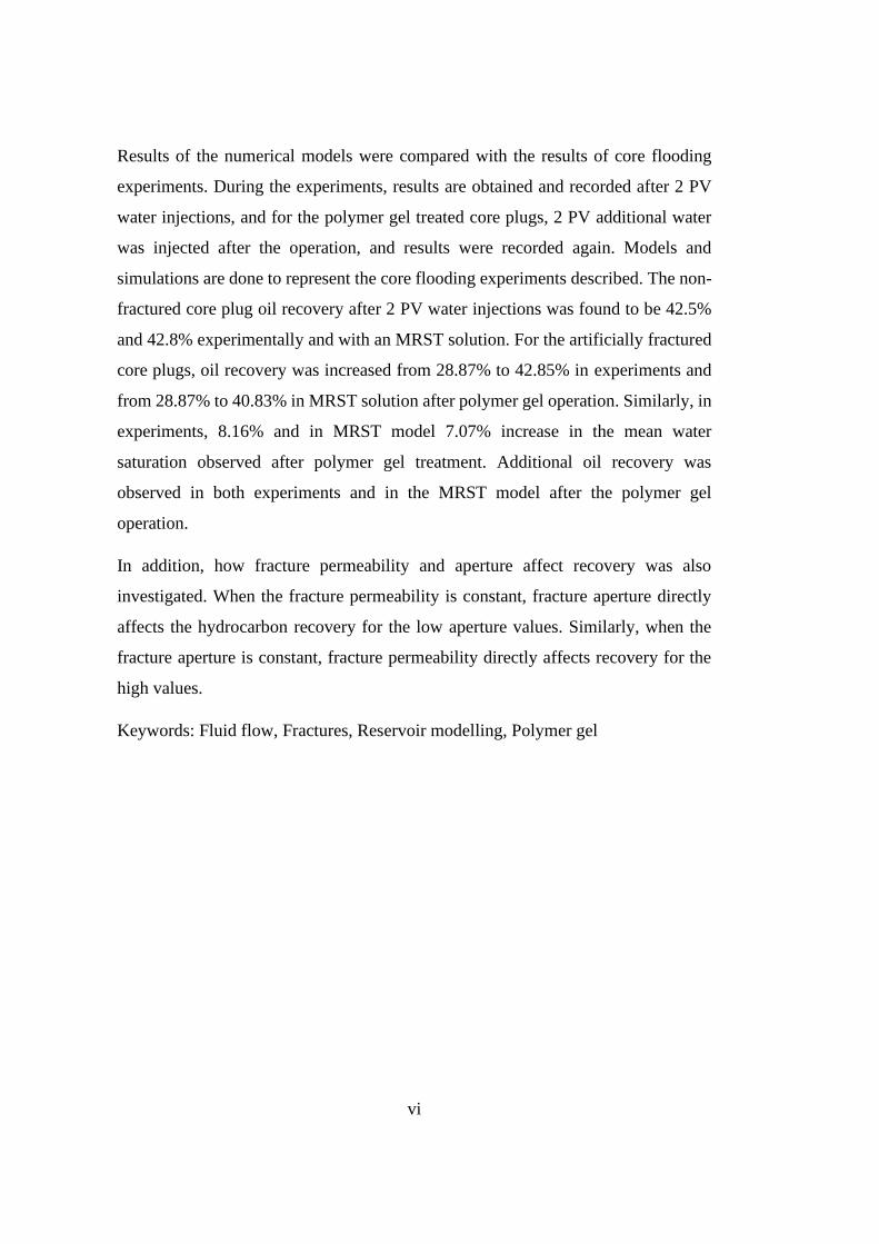
Results of the numerical models were compared with the results of core flooding
experiments. During the experiments, results are obtained and recorded after 2 PV
water injections, and for the polymer gel treated core plugs, 2 PV additional water
was injected after the operation, and results were recorded again. Models and
simulations are done to represent the core flooding experiments described. The non-
fractured core plug oil recovery after 2 PV water injections was found to be 42.5%
and 42.8% experimentally and with an MRST solution. For the artificially fractured
core plugs, oil recovery was increased from 28.87% to 42.85% in experiments and
from 28.87% to 40.83% in MRST solution after polymer gel operation. Similarly, in
experiments, 8.16% and in MRST model 7.07% increase in the mean water
saturation observed after polymer gel treatment. Additional oil recovery was
observed in both experiments and in the MRST model after the polymer gel
operation.
In addition, how fracture permeability and aperture affect recovery was also
investigated. When the fracture permeability is constant, fracture aperture directly
affects the hydrocarbon recovery for the low aperture values. Similarly, when the
fracture aperture is constant, fracture permeability directly affects recovery for the
high values.
Keywords: Fluid flow, Fractures, Reservoir modelling, Polymer gel
vii
ÖZ
YAPAY OLARAK KIRILMIŞ VE JEL İŞLEMI GÖRMÜŞ KAROTLARDA
AKIŞKAN AKIŞININ MODELLENMESI VE SIMÜLASYONU
Kaya, Onur Alp
Yüksek Lisans, Petrol ve Doğal gaz Mühendisliği
Tez Yöneticisi: Dr.Öğr. İsmail Durgut
Eylül 2021, 137 sayfa
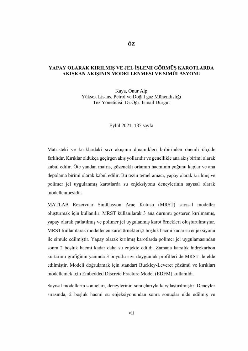
Matristeki ve kırıklardaki sıvı akışının dinamikleri birbirinden önemli ölçüde
farklıdır. Kırıklar oldukça geçirgen akış yollarıdır ve genellikle ana akış birimi olarak
kabul edilir. Öte yandan matris, gözenekli ortamın hacminin çoğunu kaplar ve ana
depolama birimi olarak kabul edilir. Bu tezin temel amacı, yapay olarak kırılmış ve
polimer jel uygulanmış karotlarda su enjeksiyonu deneylerinin sayısal olarak
modellenmesidir.
MATLAB Rezervuar Simülasyon Araç Kutusu (MRST) sayısal modeller
oluşturmak için kullanılır. MRST kullanılarak 3 ana durumu gösteren kırılmamış,
yapay olarak çatlatılmış ve polimer jel uygulanmış karot örnekleri oluşturulmuştur.
MRST kullanılarak modellenen karot örnekleri,2 boşluk hacmi kadar su enjeksiyonu
ile simüle edilmiştir. Yapay olarak kırılmış karotlarda polimer jel uygulamasından
sonra 2 boşluk hacmi kadar daha su enjekte edildi. Zamana karşılık hidrokarbon
kurtarımı grafiğinin yanında 3 boyutlu sıvı doygunluk profilleri de MRST ile elde
edilmiştir. Modeli doğrulamak için standart Buckley-Leveret çözümü ve kırıkları
modellemek için Embedded Discrete Fracture Model (EDFM) kullanıldı.
Sayısal modellerin sonuçları, deneylerinin sonuçlarıyla karşılaştırılmıştır. Deneyler
sırasında, 2 boşluk hacmi su enjeksiyonundan sonra sonuçlar elde edilmiş ve
viii
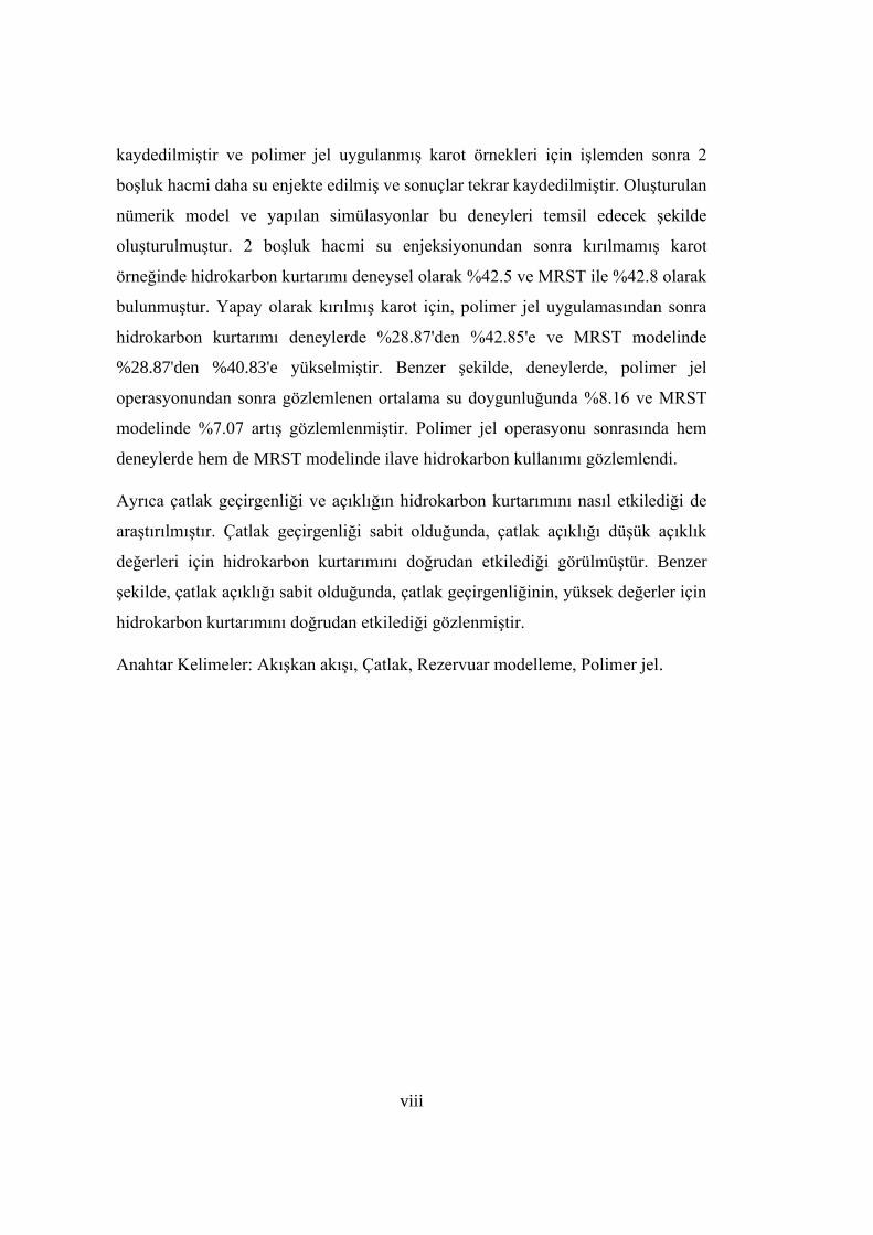
kaydedilmiştir ve polimer jel uygulanmış karot örnekleri için işlemden sonra 2
boşluk hacmi daha su enjekte edilmiş ve sonuçlar tekrar kaydedilmiştir. Oluşturulan
nümerik model ve yapılan simülasyonlar bu deneyleri temsil edecek şekilde
oluşturulmuştur. 2 boşluk hacmi su enjeksiyonundan sonra kırılmamış karot
örneğinde hidrokarbon kurtarımı deneysel olarak %42.5 ve MRST ile %42.8 olarak
bulunmuştur. Yapay olarak kırılmış karot için, polimer jel uygulamasından sonra
hidrokarbon kurtarımı deneylerde %28.87'den %42.85'e ve MRST modelinde
%28.87'den %40.83'e yükselmiştir. Benzer şekilde, deneylerde, polimer jel
operasyonundan sonra gözlemlenen ortalama su doygunluğunda %8.16 ve MRST
modelinde %7.07 artış gözlemlenmiştir. Polimer jel operasyonu sonrasında hem
deneylerde hem de MRST modelinde ilave hidrokarbon kullanımı gözlemlendi.
Ayrıca çatlak geçirgenliği ve açıklığın hidrokarbon kurtarımını nasıl etkilediği de
araştırılmıştır. Çatlak geçirgenliği sabit olduğunda, çatlak açıklığı düşük açıklık
değerleri için hidrokarbon kurtarımını doğrudan etkilediği görülmüştür. Benzer
şekilde, çatlak açıklığı sabit olduğunda, çatlak geçirgenliğinin, yüksek değerler için
hidrokarbon kurtarımını doğrudan etkilediği gözlenmiştir.
Anahtar Kelimeler: Akışkan akışı, Çatlak, Rezervuar modelleme, Polimer jel.
ix
To Infinity and Beyond

x
ACKNOWLEDGMENTS
I would like to thank my supervisor Asst. Prof. Dr. İsmail Durgut for his support,
knowledge, and guidance throughout my thesis study. Knowing that his door is
always open for help and advice was a huge encouragement for me. Without him, I
would not be able to complete my work.
I would also like to thank Prof. Dr. Mahmut Parlaktuna and Asst. Prof. Dr. Doruk
Alp for their valuable recommendations and their involvement in my examining
committee.
My deepest thanks belong to my family. My beloved parents Mustafa and Emine
Kaya, my brother and my sister-in-law Mehmet Ferda and Gözde, and the loudest
and sweetest member of the family Berfu, without you and your support, I would not
be the person I am today. Knowing that you will always be there for me whenever I
needed is the biggest and most comforting thing I have in my life. Thank you so
much.
I want to thank my colleague, my role model in the department, and most
importantly, my friend Rabia Tuğçe Özdemir for her support and the good times we
spent.
My friends Mami, Yılmaz, Harun, Batu, Mehri, Egemen, Muslu thanks for being
there with me, and being the best company, I can ever imagine.
Last but not least, I would like to thank Sıla for her continuous support and
encouragement through the processes of writing this thesis and especially running
the simulations. Thanks to you, I found the energy to run the simulations again and
again. You made this whole journey more colorful and enjoyable.
xi
TABLE OF CONTENTS
ABSTRACT ............................................................................................................... v
ÖZ ........................................................................................................................... vii
ACKNOWLEDGMENTS ......................................................................................... x
TABLE OF CONTENTS ......................................................................................... xi
LIST OF TABLES ................................................................................................. xiii
LIST OF FIGURES ............................................................................................... xiv
1 INTRODUCTION ............................................................................................. 1
2 RESERVOIR ROCK STUDIES AND PROPERTIES ...................................... 5
2.1 Core Plug Studies ............................................................................................ 5
3 FRACTURED POROUS MEDIA ................................................................... 11
3.1 Darcy’s Law .................................................................................................. 11
3.2 Fluid Flow in Fractures ................................................................................. 13
3.3 Fractures and Fracture Modelling ................................................................. 15
3.4 Types of Statistical Distributions .................................................................. 20
4 WATER FLOODING EXPERIMENTS ......................................................... 25
4.1 Core Plug Experiments ................................................................................. 25
4.2 Water Flooding Experiments ........................................................................ 26
4.3 Results of the Experiments ........................................................................... 29
5 STATEMENT OF PROBLEM ........................................................................ 35
6 NUMERICAL MODELLING ......................................................................... 37
6.1 MATLAB Reservoir Simulation Toolbox (MRST) ..................................... 37
6.2.1 Automatic Differentiation (AD) ................................................................ 38
xii
6.2.2 Two Point Flux Approximation ................................................................ 39
6.3 Modelling the Non-Fractured/Non-Gel Treated Core Plug#8 ...................... 41
6.4 Modelling of Fractured and Gel Treated Core Plugs ................................... 47
7 VALIDATION OF MODEL ........................................................................... 53
7.1 General Buckley-Leveret Solution ............................................................... 53
8 RESULTS AND DISCUSSION ...................................................................... 67
8.1 Core Plug#8 .................................................................................................. 67
8.2 Core Plug#2 .................................................................................................. 71
8.3 Core Plug#3 .................................................................................................. 74
8.4 Core Plug#7 .................................................................................................. 80
8.5 Core Plug#5 .................................................................................................. 86
8.6 Fracture Permeability and Aperture ............................................................. 92
9 CONCLUSION ............................................................................................... 95
REFERENCES ........................................................................................................ 97
A. MATLAB CODES ........................................................................................ 103
xiii
LIST OF TABLES
TABLES
Table 1: General structure of core plugs ................................................................. 25
Table 2: Fluid properties ......................................................................................... 45
Table 3: Comparison of selected values for MRST model and actual case ............ 47
Table 4: Comparison of the important parameters for core plug#2 ........................ 50
Table 5:Comparison of the important parameters for core plug#3 ......................... 51
Table 6:Comparison of the important parameters for core plug#5 ......................... 51
Table 7: Comparison of the important parameters for core plug#7 ........................ 51
Table 8: Comparison of the important parameters for core plug#8 ........................ 52
Table 9: Summary of core plug#8........................................................................... 70
Table 10: Summary of core plug#2......................................................................... 73
Table 11: Summary of core plug#3......................................................................... 80
Table 12: Summary of core plug#7......................................................................... 86
Table 13: Summary of core plug#5......................................................................... 92
xiv
LIST OF FIGURES
FIGURES
Figure 1: Wettability(Abdallah et al., n.d.) ............................................................... 6
Figure 2: Typical capillary pressure curve (Malik, 2017) ......................................... 7
Figure 3: Corey type relative permeability curves .................................................... 8
Figure 4: Illustration of the Darcy Experiment (Lie, 2019) .................................... 11
Figure 5: Fluid flow between two parallel plates .................................................... 13
Figure 6: Effect of fractures on the modelling (Lei et al., 2017) ............................. 16
Figure 7: Dual-porosity, dual-permeability model(Warren & Root, 1963) ............ 17
Figure 8: Discrete Fracture Model (DFM) .............................................................. 18
Figure 9: 2D and 3D Poisson DFN models (Lei et al., 2017) ................................. 19
Figure 10: Embedded Discrete Fracture Model (EDFM) (Ţene et al., 2017) ......... 19
Figure 11: PDF’s for different distribution methods (Shiriyev, 2013) .................... 21
Figure 12: Polymer gel treatment (Zhang et al., 2020) ........................................... 23
Figure 13: CT Scans ................................................................................................ 26
Figure 14:Experimental set-up of ................................................................................
Figure 15: Outlet pressure profile of core plug#2 ................................................... 28
Figure 16: Experimental water saturation profile of core plug#2 ...............................
Figure 17: Experimental water saturation profile of core plug#3 ...............................
Figure 18:Experimental water saturation profile of core plug#5 ............................ 30
Figure 19:Experimental water saturation profile of core plug#7 ............................ 30
Figure 20:Experimental water saturation profile of core plug#8 ............................ 31
Figure 21:Recovery vs Time plot of core samples .................................................. 32
Figure 22:Recovery vs PV Injected plot of core samples ....................................... 32
Figure 23: General framework of MRST (Lie, 2019) ............................................. 37
Figure 24: Mini-step solution procedure of AD (Lie, 2019) ................................... 39
Figure 25: Schematic visualization of TPFA .......................................................... 39
Figure 26: Base grid structure of core plug#8 ......................................................... 42
Figure 27: Grid structure of core plug#8 ................................................................. 43
xv
Figure 28: Permeability distribution of core plug#8 ............................................... 44
Figure 29: Porosity distribution of core plug#8 ...................................................... 45
Figure 30: Relative permeability curves for the core plug#8.................................. 46
Figure 31: Initial oil and water saturation distributions for core plug#8 ................ 46
Figure 32: Fracture plane ........................................................................................ 48
Figure 33: Fracture grid .......................................................................................... 48
Figure 34: Matrix-fracture NNC's ........................................................................... 49
Figure 35: Procedure for fractured and gel-treated core plug modelling ................ 50
Figure 36: Typical fractional flow curve ................................................................ 54
Figure 37: Typical frontal advance profile for waterflooding ................................ 56
Figure 38: Water saturation vs fractional flow ....................................................... 57
Figure 39: Derivative term vs water saturation ....................................................... 57
Figure 40:Analytical solution of the waterfront location ........................................ 58
Figure 41: Comparison of the analytical and MRST model solution ..................... 58
Figure 42: Overall comparison of analytical and MRST solution for the waterfront
advance ................................................................................................................... 59
Figure 43: Approximate solutions computed by the explicit transport solver and the
implicit transport solver with n time steps .............................................................. 60
Figure 44:Waterfront location for different solution methods (4000 cells) ............ 61
Figure 45:Waterfront location for different solution methods (2000 cells) ............ 61
Figure 46:Waterfront location for different solution methods (1000 cells) ............ 62
Figure 47:Waterfront location for different solution methods (400 cells) .............. 62
Figure 48:Waterfront location for different solution methods (100 cells) .............. 63
Figure 49: Waterfront location for explicit solution vs analytical solution for
different cell numbers ............................................................................................. 63
Figure 50:Waterfront location for implicit solution vs analytical solution for
different cell numbers ............................................................................................. 64
Figure 51:Waterfront location for MRST solution vs analytical solution for
different cell numbers ............................................................................................. 64
xvi
Figure 52: Oil saturation distribution of core plug#8 (top left 0.2 PV, top middle
0.5 PV, top right 1 PV, bottom left 1.4 PV, bottom middle 1.7 PV and bottom right
2.0 PV) ..................................................................................................................... 68
Figure 53:Water saturation distribution of core plug#8 (top left 0.2 PV, top middle
0.5 PV, top right 1 PV, bottom left 1.4 PV, bottom middle 1.7 PV and bottom right
2.0 PV) ..................................................................................................................... 68
Figure 54: Water saturation profile of core plug#8 ................................................. 69
Figure 55: Recovery vs Time plot of core plug#8 ................................................... 70
Figure 56: Water saturation distribution of core plug#2 (top left 0.2 PV, top middle
0.5 PV, top right 1 PV, bottom left 1.4 PV, bottom middle 1.7 PV and bottom right
2.0 PV) ..................................................................................................................... 71
Figure 57: Water saturation distribution of core plug#2 (top left 0.2 PV, top middle
0.5 PV, top right 1 PV, bottom left 1.4 PV, bottom middle 1.7 PV and bottom right
2.0 PV) ..................................................................................................................... 72
Figure 58: Water saturation profile of core plug#2 ................................................. 72
Figure 59: Recovery vs Time plot of core plug#2 ................................................... 73
Figure 60: Water saturation distribution of core plug#3 before polymer gel
treatment (top left 0.2 PV, top middle 0.5 PV, top right 1 PV, bottom left 1.4 PV,
bottom middle 1.7 PV and bottom right 2.0 PV) .................................................... 74
Figure 61: Oil saturation distribution of core plug#3 before polymer gel treatment
(top left 0.2 PV, top middle 0.5 PV, top right 1 PV, bottom left 1.4 PV, bottom
middle 1.7 PV and bottom right 2.0 PV) ................................................................. 75
Figure 62: Water saturation profile of core plug#3 before polymer gel treatment . 76
Figure 63: Recovery vs Time plot of core plug#3 before polymer gel treatment ... 76
Figure 64: Water saturation distribution of core plug#3 after polymer gel treatment
(top left 0.2 PV, top middle 0.5 PV, top right 1 PV, bottom left 1.4 PV, bottom
middle 1.7 PV and bottom right 2.0 PV) ................................................................. 77
Figure 65: Oil saturation distribution of core plug#3 after polymer gel treatment
(top left 0.2 PV, top middle 0.5 PV, top right 1 PV, bottom left 1.4 PV, bottom
middle 1.7 PV and bottom right 2.0 PV) ................................................................. 78
xvii
Figure 66: Final water saturation profile of core plug#3 after polymer gel treatment
................................................................................................................................. 79
Figure 67: Overall Recovery vs Time plot of core plug#3 ..................................... 79
Figure 68: Water saturation distribution of core plug#7 before polymer gel
treatment (top left 0.2 PV, top middle 0.5 PV, top right 1 PV, bottom left 1.4 PV,
bottom middle 1.7 PV and bottom right 2.0 PV) .................................................... 81
Figure 69: Oil saturation distribution of core plug#3 before polymer gel treatment
(top left 0.2 PV, top middle 0.5 PV, top right 1 PV, bottom left 1.4 PV, bottom
middle 1.7 PV and bottom right 2.0 PV) ................................................................ 81
Figure 70: Water saturation profile of core plug#7 before polymer gel treatment . 82
Figure 71: Recovery vs Time plot of core plug#7 before polymer gel treatment ... 82
Figure 72: Water saturation distribution of core plug#7 after polymer gel treatment
(top left 0.2 PV, top middle 0.5 PV, top right 1 PV, bottom left 1.4 PV, bottom
middle 1.7 PV and bottom right 2.0 PV) ................................................................ 83
Figure 73: Oil saturation distribution of core plug#7 after polymer gel treatment
(top left 0.2 PV, top middle 0.5 PV, top right 1 PV, bottom left 1.4 PV, bottom
middle 1.7 PV and bottom right 2.0 PV) ................................................................ 84
Figure 74: Water saturation profile of core plug#7 after polymer gel treatment .... 84
Figure 75: Overall recovery vs time plot of core plug#7 ........................................ 85
Figure 76: Water saturation distribution of core plug#5 before polymer gel
treatment (top left 0.2 PV, top middle 0.5 PV, top right 1 PV, bottom left 1.4 PV,
bottom middle 1.7 PV and bottom right 2.0 PV) .................................................... 87
Figure 77: Oil saturation distribution of core plug#5 before polymer gel treatment
(top left 0.2 PV, top middle 0.5 PV, top right 1 PV, bottom left 1.4 PV, bottom
middle 1.7 PV and bottom right 2.0 PV) ................................................................ 87
Figure 78: Water saturation profile of core plug#5 before polymer gel treatment . 88
Figure 79: Recovery vs time plot of core plug#7 before polymer gel operation .... 89
Figure 80: Water saturation distribution of core plug#5 after polymer gel treatment
(top left 0.2 PV, top middle 0.5 PV, top right 1 PV, bottom left 1.4 PV, bottom
middle 1.7 PV and bottom right 2.0 PV) ................................................................ 90
xviii
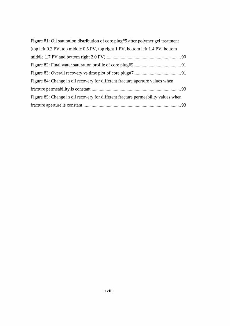
Figure 81: Oil saturation distribution of core plug#5 after polymer gel treatment
(top left 0.2 PV, top middle 0.5 PV, top right 1 PV, bottom left 1.4 PV, bottom
middle 1.7 PV and bottom right 2.0 PV) ................................................................. 90
Figure 82: Final water saturation profile of core plug#5 ......................................... 91
Figure 83: Overall recovery vs time plot of core plug#7 ........................................ 91
Figure 84: Change in oil recovery for different fracture aperture values when
fracture permeability is constant ............................................................................. 93
Figure 85: Change in oil recovery for different fracture permeability values when
fracture aperture is constant ..................................................................................... 93
1
CHAPTER 1
1 INTRODUCTION
Hydrocarbon production from the reservoirs is based on the fluid flow in the porous
medium. Modeling of the fluid flow in porous media can be challenging due to the
heterogeneities involved. Natural or artificial fractures are one of these
heterogeneities.
Fractures are long wide flow channels in the reservoirs. The physical structure of
fractures is significantly different than the matrix. Thus, their existence has a strong
influence on reservoir flow dynamics. Therefore, understanding the effects of
fractures on hydrocarbon production from underground is crucial.
Fluid flow in the fracture is significantly different from the matrix. The matrix
occupies the most volume of the porous media; therefore, the matrix is considered
the main storage unit, and fractures are considered the main flow channels. Flow
dynamics in the matrix and fracture is different, so it is crucial to create a model that
accurately represents both the fracture and matrix of the porous medium. Various
models like continuum model, dual-porosity model, dual-porosity dual-permeability
model, discrete fracture model (DFM), and embedded discrete fracture model
(EDFM) are available with different advantages and disadvantages.
This study focuses on the effects of fractures and polymer gel treatment on the
hydrocarbon recovery in the core scale. Experimentally obtained recovery values for
different conditions are compared with the results of the mathematical model.
Experimental data was obtained from the Ph.D dissertation of Dr.Serhat Canbolat.
In addition, publicly available data in two papers written by him and Dr. Mahmut
Parlaktuna were used.
2
Experimental and numerical results of oil recovery for normal, naturally fractured,
artificially fractured and polymer gel treated core samples are compared. In addition,
the effects of fracture permeability and aperture on the recovery are investigated.
Mathematical modeling and simulations are done by using MATLAB Reservoir
Simulation Toolbox (MRST), which is open-source software for reservoir modeling
and simulation.
The structure of the thesis is as follows.
Chapter 2: This chapter provides theoretical information about the main reservoir
rock properties. Properties mentioned in this chapter greatly impact modeling the
core plug and oil recovery from it. In addition to core plug studies, wettability,
capillary pressure, and relative permeability and their effect on the modeling are
briefly explained.
Chapter 3: In this chapter, the main equations of fluid flow in porous medium and
fractured porous medium are described. Different fracture models with their upsides
and downsides are explained, and finally, the effect of the polymer gel treatment on
the reservoir rock properties and hydrocarbon production is presented.
Chapter 4: Waterflooding experiments are explained in this chapter. Initially, basic
information related to core plugs that are used in the experiments were given. Then,
how the experiments are conducted explained and finally results of the experiments
provided in this chapter.
Chapter 5: The statement of the problem is explained in this section.
Chapter 6: After providing necessary theoretical background information about the
modeling of fluid flow in porous and fractured medium, 3D modeling of the problem
in MRST is explained. In this chapter. Initially, theoretical information about MRST
and the boundary conditions, and the mathematical principle of the used functions
are explained. Procedure for the physical modeling of fractured and non-fractured
core plugs explained step by step.
3
Chapter 7. In this chapter, validation of the MRST model is done. Initially,
theoretical information about the analytical Buckley-Leveret solution as wells as the
general solution procedure is explained. Then a base model is solved both by MRST
and Buckley-Leveret solution and obtained results of the numerical model, and the
analytical solution is compared to validate the model.
Chapter 8: In this chapter, waterflooding to all core plug models created, are
simulated by MRST. Experimental and model results are compared for fractured and
gel-treated cases. In addition, the effects of the fracture aperture and fracture
permeability on hydrocarbon recovery are investigated. Obtained results are
discussed and compared with the literature.
Chapter 9: In this chapter, the work done is concluded, and final ideas are provided.
In addition, possible future work is mentioned.

5
CHAPTER 2
2 RESERVOIR ROCK STUDIES AND PROPERTIES
2.1 Core Plug Studies
Core plug studies are one of the most fundamental studies in petroleum and natural
gas engineering. Since it is impossible to work with wholly known reservoirs, small
representative specimens from the reservoirs are needed to obtain data. These
samples are known as core plugs. It is possible to obtain various information about
reservoir properties by conducting necessary experiments on core plugs.
Fundamental properties like porosity, permeability, and fluid saturation of the rock
and relative permeability, capillary pressure, secondary and enhanced oil recovery
studies (waterflooding, CO2 injection, thermal recovery) are all can be conducted in
these core plugs. Data obtained from core plugs are used to accurately model the
reservoir and run some simulations for the possible activities.
2.2 Wettability
An important reservoir rock property for oil recovery is the wettability of the
reservoir. Wettability can be defined as the rock's preference to be in contact with a
specific fluid (AlSofi & Yousef, 2013). In oil-wet reservoirs, pore surfaces are in
contact with petroleum. Similarly, water is the covering phase for water-wet
reservoirs. Since oil is covering the rock surface, expected oil recovery is lower in
oil-wet systems. It is possible to have mixed-wet reservoir rocks where both oil and
water cover the rock surface, and they are both placed in the center of the pores at
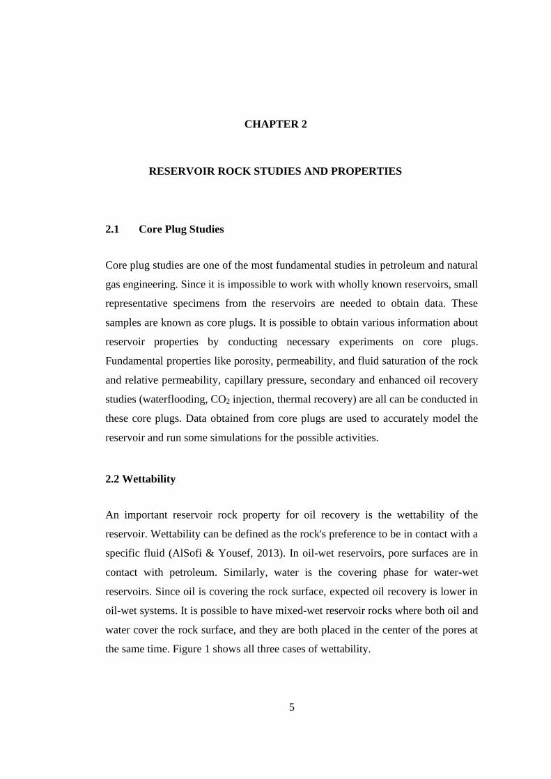
the same time. Figure 1 shows all three cases of wettability.
6
Figure 1: Wettability(Abdallah et al., n.d.)
Generally, reservoir rocks were water-wet before the migration of oil. Due to this
migration, a gradual saturation change is expected in a reservoir from the free water
level at the bottom to the irreducible water saturation at the top (Chen et al., 2018).
This fluid saturation change along the reservoir leads to a pressure difference
between the wetting and non-wetting phase, and this pressure difference is known as
the capillary pressure.
2.3 Capillary Pressure
Capillary pressure is another critical term for two-phase flow in porous media. When
two immiscible fluids exist across an interface, pressure discontinuity happens. This
discontinuity in the pressure is called capillary pressure (Iglauer, 2017). Another
definition of capillary pressure is the pressure difference between the non-wetting
phase and the wetting phase.
𝑃𝑐 = 𝑃𝑛𝑤 − 𝑃𝑤 (2.1)
Physical expression of the capillary pressure is as following:
𝑃𝑐 =2𝜎𝑜𝑤cos(𝜃)
𝑟 (2.2)
7
Where 𝜎𝑜𝑤 is the interfacial tension between oil and water and cos(𝜃) is the wetting
degree angle and r is the effective radius interface (radius of capillarity).
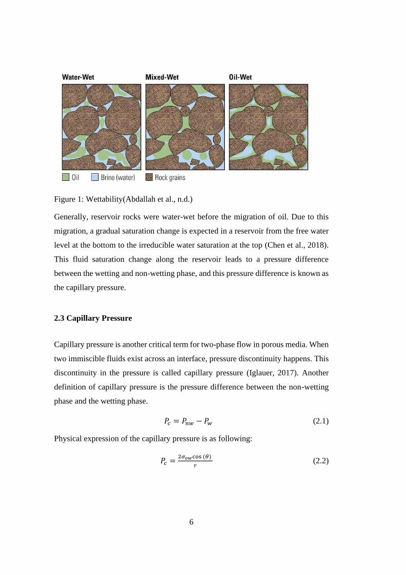
The only way to obtain capillary pressure data for a medium is through laboratory
studies (Morrow, 1962; Nojabaei et al., 2013). Different models are available to
generalize capillary pressure data. Capillary pressure directly affects fluid flow by
controlling the direction and movements of the reservoir liquids. Therefore, the free
water level of the reservoir, threshold pressure required to mobilize water, immobile
water saturation can be seen in the capillary pressure curve. Figure 2 shows a sample
capillary pressure curve.
Figure 2: Typical capillary pressure curve (Malik, 2017)
2.4 Relative Permeability
Permeability of a rock can be defined as the rock's ability to permit fluid flow. The
distribution of the pores, pore throats can affect the permeability of the rock.
Absolute permeability is a rock property, and it is a constant value. However,
effective permeability depends on the types of fluids. Having two different phases
simultaneously in the same medium affects the permeability of those two phases.
Water flow along the medium in the presence of oil, cannot be the same as the case
8
of only water-saturated medium. The relative permeability concept explains this
phenomenon. Relative permeability can be obtained by dividing the effective
permeability of one phase by the absolute permeability of the same phase. The
relative permeability of a phase is always between 0 and 1.
𝑘𝑟𝑒𝑙 =𝑘𝑒𝑓𝑓
𝑘𝑎𝑏𝑠 (2.3)
For reservoir engineering purposes, like waterflooding of the reservoir, or CO2
injection, relative permeability of phases has crucial importance on the efficiency of
these applications (Johnson et al., 1959). Endpoints of the relative permeability
curves show theoretical maximum and minimum phase saturations in the rock.
Although knowing relative permeability curves is essential, it is not always possible.
There are some models available for estimating the relative permeability curves
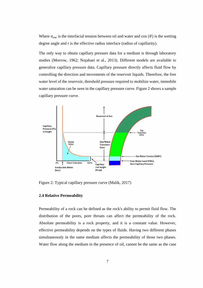
(Bryant & Blunt, 1992). Corey's model is one of the most used and common one.
Typical Corey model relative permeability curves can be seen in figure 3.
Figure 3: Corey type relative permeability curves
9
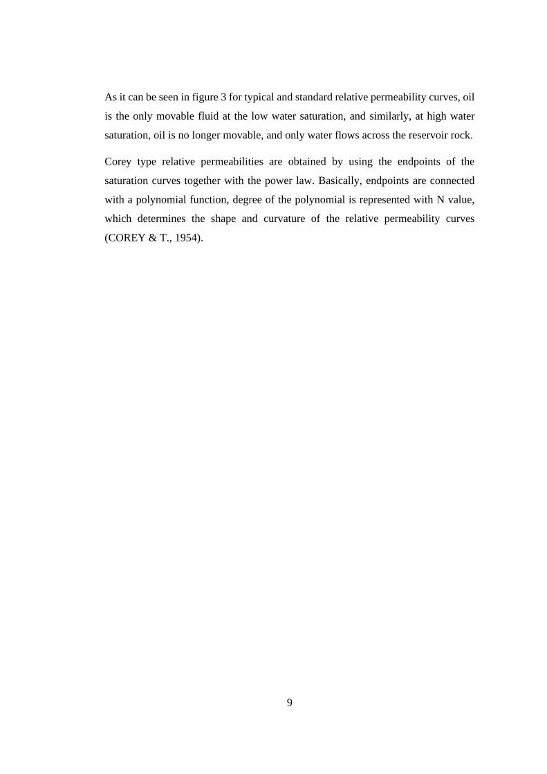
As it can be seen in figure 3 for typical and standard relative permeability curves, oil
is the only movable fluid at the low water saturation, and similarly, at high water
saturation, oil is no longer movable, and only water flows across the reservoir rock.
Corey type relative permeabilities are obtained by using the endpoints of the
saturation curves together with the power law. Basically, endpoints are connected
with a polynomial function, degree of the polynomial is represented with N value,
which determines the shape and curvature of the relative permeability curves
(COREY & T., 1954).

11
CHAPTER 3
3 FRACTURED POROUS MEDIA
3.1 Darcy’s Law
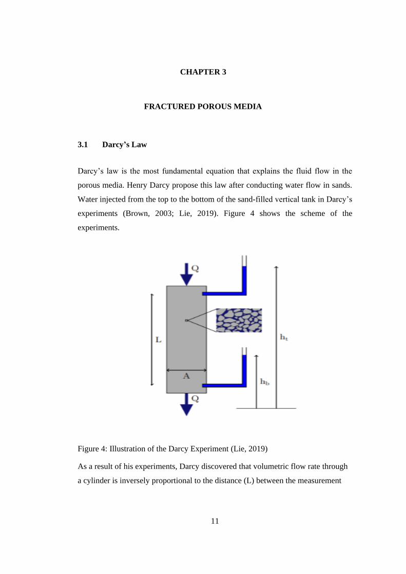
Darcy’s law is the most fundamental equation that explains the fluid flow in the
porous media. Henry Darcy propose this law after conducting water flow in sands.
Water injected from the top to the bottom of the sand-filled vertical tank in Darcy’s
experiments (Brown, 2003; Lie, 2019). Figure 4 shows the scheme of the
experiments.
Figure 4: Illustration of the Darcy Experiment (Lie, 2019)
As a result of his experiments, Darcy discovered that volumetric flow rate through
a cylinder is inversely proportional to the distance (L) between the measurement
12
locations and proportional to the difference in hydraulic head (ℎ𝑡𝑎𝑛𝑑ℎ𝑏) and
cross-sectional area (A).
General form of the Darcy’s law is as following.
𝑄 = 𝐴 × 𝐾 ×(ℎ𝑡−ℎ𝑏)
𝐿 (3.1)
𝑄
𝐴= 𝐾 ×
ℎ𝑡−ℎ𝑏
𝐿 (3.2)
Where 𝑄 is the discharge, K is the hydraulic conductivity, A is the cross-sectional
area, h values are hydraulic head for given elevations, k is the permeability, g is the
gravitational acceleration and 𝜇 and 𝜌 are the viscosity and density of the fluid.
Assuming constant permeability in every direction, then generally hydraulic
conductivity becomes a tensor which is represented as
𝐾 = 𝑘 × 𝜌 × 𝑔
𝜇 (3.3)
Where q is the fluid flux vector and ∇h is the gradient for the hydraulic head.
Representing the hydraulic head at a point as
ℎ =𝑝
𝜌×𝑔+ 𝑧(3.4)
where z is the elevation relative to a defined datum.
Representing the equation 3.1 in a differential form by using equations 3.3 and 3.4
leads to:
𝑣 = −𝐾∇ℎ = −1
𝜇𝑘(∇𝑝 − 𝜌𝑔∇𝑧)(3.5)
Equation 3.5 is generally considered as the modern form of the Darcy equation. 𝑣
is the volumetric flux called Darcy velocity.
13
3.2 Fluid Flow in Fractures
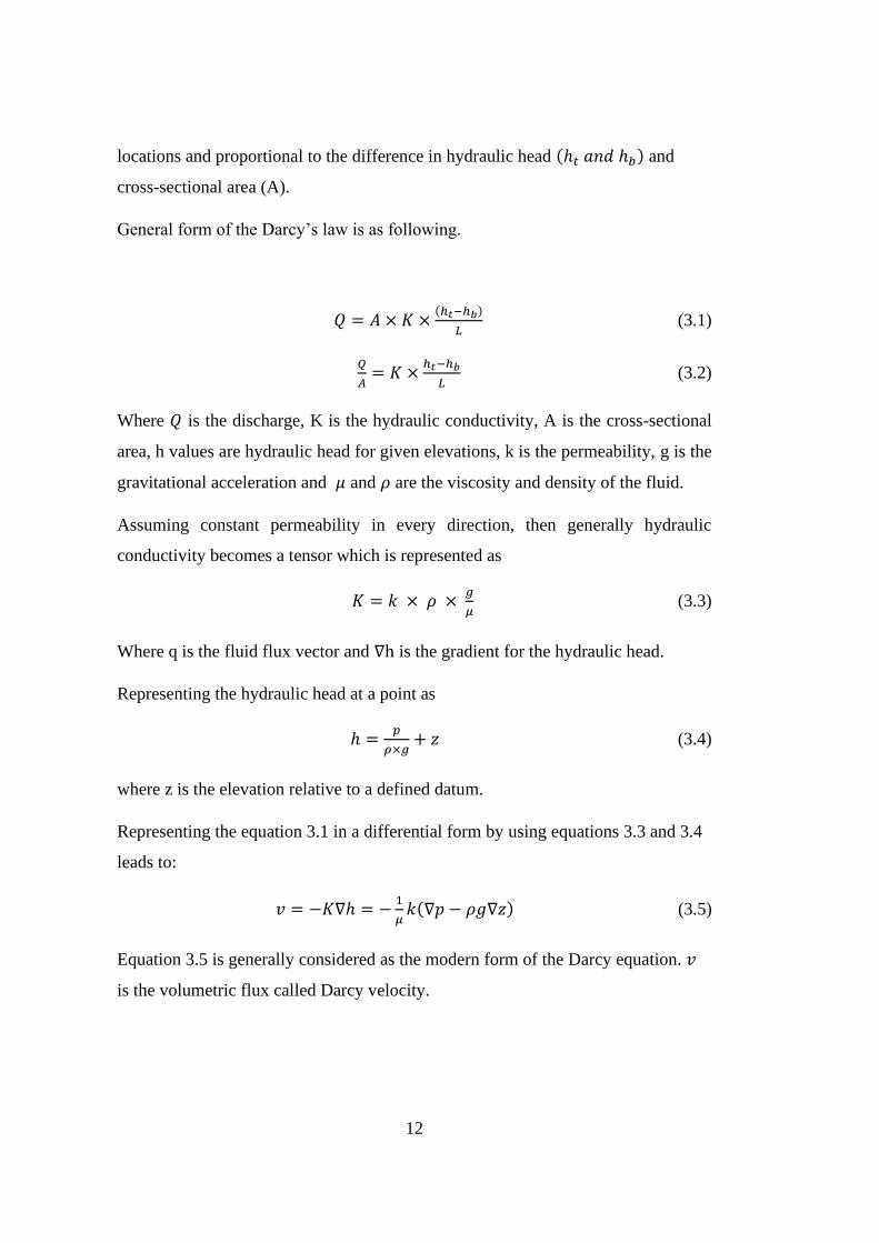
Fractures are long flow paths in the matrix with a certain width. Fluid flow in the
fractures can be similar to the fluid flow in the two smooth parallel plates. Figure 5
illustrates the laminar fluid flow between two parallel plates.
Figure 5: Fluid flow between two parallel plates
Cubic law is the most common way to express the fluid flow under mentioned
circumstances. To obtain the well-known cubic law, the Navier-Stokes equation for
incompressible flow given below needs to be solved
𝜌 (𝜕�⃗�
𝜕𝑡+ 𝑣 ∇𝑣 ) = −∇𝑝 + 𝜇∇ 𝑣⃗⃗⃗ (3.6)
Assuming steady-state conditions, no-slip conditions at the top and bottom, as well
as ignoring gravity, introducing constant fracture aperture b, and finally assuming
constant pressure at the boundaries, inlet pressure 𝑝1 is greater or equal to outlet
pressure 𝑝2, equation 3.6 becomes
𝑝1−𝑝2
𝐿+ 𝜇
𝜕2𝑣𝑦
𝜕2𝑧2 = 0 (3.7)
In parallel plate assumption, flow only happens in y direction, and it is equal to zero
for the other directions. Integrating equation twice, and imposing the boundary
conditions, will lead to velocity field
14
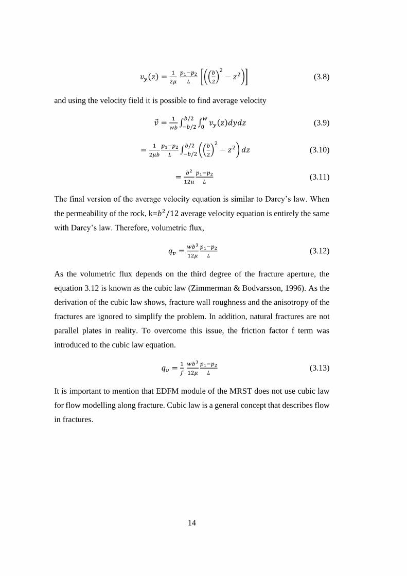
𝑣𝑦(𝑧) =1
2𝜇𝑝1−𝑝2
𝐿[((
𝑏
2)2
− 𝑧2)] (3.8)
and using the velocity field it is possible to find average velocity
𝑣 =1
𝑤𝑏∫ ∫ 𝑣𝑦(𝑧)𝑑𝑦𝑑𝑧
𝑤
0
𝑏/2
−𝑏/2 (3.9)
=1
2𝜇𝑏
𝑝1−𝑝2
𝐿∫ ((
𝑏
2)2
− 𝑧2) 𝑑𝑧𝑏/2
−𝑏/2 (3.10)
=𝑏2
12𝑢
𝑝1−𝑝2
𝐿 (3.11)
The final version of the average velocity equation is similar to Darcy’s law. When
the permeability of the rock, k=𝑏2/12average velocity equation is entirely the same
with Darcy’s law. Therefore, volumetric flux,
𝑞𝑣 =𝑤𝑏3
12𝜇
𝑝1−𝑝2
𝐿 (3.12)
As the volumetric flux depends on the third degree of the fracture aperture, the
equation 3.12 is known as the cubic law (Zimmerman & Bodvarsson, 1996). As the
derivation of the cubic law shows, fracture wall roughness and the anisotropy of the
fractures are ignored to simplify the problem. In addition, natural fractures are not
parallel plates in reality. To overcome this issue, the friction factor f term was
introduced to the cubic law equation.
𝑞𝑣 =1
𝑓𝑤𝑏3
12𝜇
𝑝1−𝑝2
𝐿 (3.13)
It is important to mention that EDFM module of the MRST does not use cubic law
for flow modelling along fracture. Cubic law is a general concept that describes flow
in fractures.
15
3.3 Fractures and Fracture Modelling
Fractures are high permeability flow channels that can exist in reservoirs. There can
be km long, and significantly wide with a complex structure for a reservoir, or a
single, few cm long in a core sample. However, existence of a fracture completely
changes the flow patterns regardless of its physical properties. In the presence of a
fracture, the matrix rock acts as a storage unit, and the main fluid flow happens in
the fractures. Flow dynamics of these two units are different from each other, and
fluid flow between the fracture and rock is commonly observed (Nazridoust et al.,
2006; Ranjith et al., 2006). Fluid interactions between these two different units are
also different from matrix-matrix and fracture-fracture interaction. That is why
fractures create heterogeneities that makes reservoir modeling more complex and
demanding. Knowing the exact locations and properties of these fractures are
essential to get valid results for the simulations.
Fracture modeling is different than regular matrix modeling as fractures and matrix
has different features. Representation of fractures in a model is crucial to get a
accurate results (R. Liu et al., 2016). There are several difficulties to model natural
fractures properly. As natural fractures occur under the in-situ pressure at the
reservoir, breakage and fragmentation can occur at any stage and level of reservoir.
Direction, distance, aperture, etc.. of the fractures are hard to detect for this reason.
Significant effort and expensive methods (like 3D borehole imaging) are required to
overcome this problem (Lei et al., 2017). Figure 6 shows the representation of the
model with and without fractures.
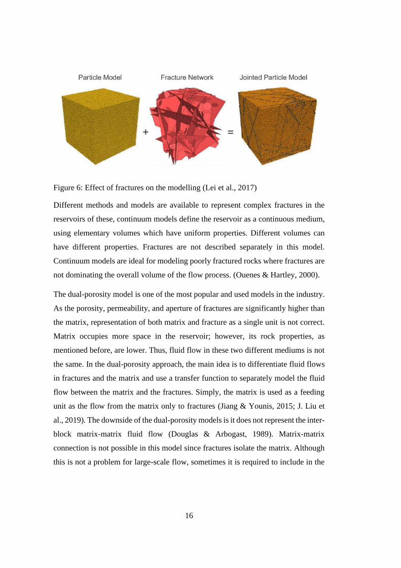
16
Figure 6: Effect of fractures on the modelling (Lei et al., 2017)
Different methods and models are available to represent complex fractures in the
reservoirs of these, continuum models define the reservoir as a continuous medium,
using elementary volumes which have uniform properties. Different volumes can
have different properties. Fractures are not described separately in this model.
Continuum models are ideal for modeling poorly fractured rocks where fractures are
not dominating the overall volume of the flow process. (Ouenes & Hartley, 2000).
The dual-porosity model is one of the most popular and used models in the industry.
As the porosity, permeability, and aperture of fractures are significantly higher than
the matrix, representation of both matrix and fracture as a single unit is not correct.
Matrix occupies more space in the reservoir; however, its rock properties, as
mentioned before, are lower. Thus, fluid flow in these two different mediums is not
the same. In the dual-porosity approach, the main idea is to differentiate fluid flows
in fractures and the matrix and use a transfer function to separately model the fluid
flow between the matrix and the fractures. Simply, the matrix is used as a feeding
unit as the flow from the matrix only to fractures (Jiang & Younis, 2015; J. Liu et
al., 2019). The downside of the dual-porosity models is it does not represent the inter-
block matrix-matrix fluid flow (Douglas & Arbogast, 1989). Matrix-matrix
connection is not possible in this model since fractures isolate the matrix. Although
this is not a problem for large-scale flow, sometimes it is required to include in the
17
model. In addition, the matrix is assumed to have constant properties, which is not
the case most of the time.
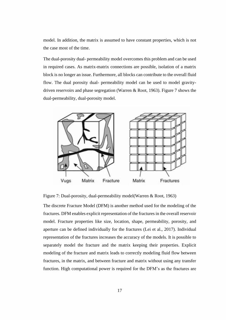
The dual-porosity dual- permeability model overcomes this problem and can be used
in required cases. As matrix-matrix connections are possible, isolation of a matrix
block is no longer an issue. Furthermore, all blocks can contribute to the overall fluid
flow. The dual porosity dual- permeability model can be used to model gravity-
driven reservoirs and phase segregation (Warren & Root, 1963). Figure 7 shows the
dual-permeability, dual-porosity model.
Figure 7: Dual-porosity, dual-permeability model(Warren & Root, 1963)
The discrete Fracture Model (DFM) is another method used for the modeling of the
fractures. DFM enables explicit representation of the fractures in the overall reservoir
model. Fracture properties like size, location, shape, permeability, porosity, and
aperture can be defined individually for the fractures (Lei et al., 2017). Individual
representation of the fractures increases the accuracy of the models. It is possible to
separately model the fracture and the matrix keeping their properties. Explicit
modeling of the fracture and matrix leads to correctly modeling fluid flow between
fractures, in the matrix, and between fracture and matrix without using any transfer
function. High computational power is required for the DFM’s as the fractures are
18
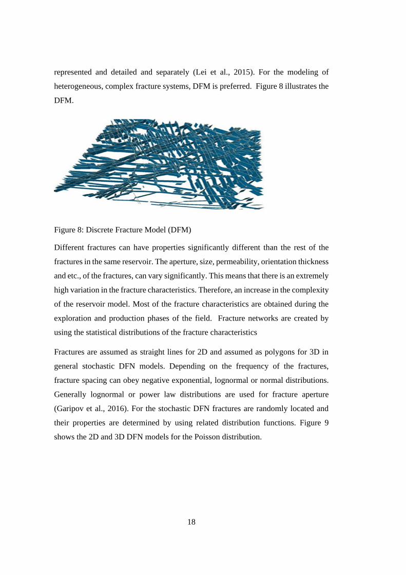
represented and detailed and separately (Lei et al., 2015). For the modeling of
heterogeneous, complex fracture systems, DFM is preferred. Figure 8 illustrates the
DFM.
Figure 8: Discrete Fracture Model (DFM)
Different fractures can have properties significantly different than the rest of the
fractures in the same reservoir. The aperture, size, permeability, orientation thickness
and etc., of the fractures, can vary significantly. This means that there is an extremely
high variation in the fracture characteristics. Therefore, an increase in the complexity
of the reservoir model. Most of the fracture characteristics are obtained during the
exploration and production phases of the field. Fracture networks are created by
using the statistical distributions of the fracture characteristics
Fractures are assumed as straight lines for 2D and assumed as polygons for 3D in
general stochastic DFN models. Depending on the frequency of the fractures,
fracture spacing can obey negative exponential, lognormal or normal distributions.
Generally lognormal or power law distributions are used for fracture aperture
(Garipov et al., 2016). For the stochastic DFN fractures are randomly located and
their properties are determined by using related distribution functions. Figure 9
shows the 2D and 3D DFN models for the Poisson distribution.
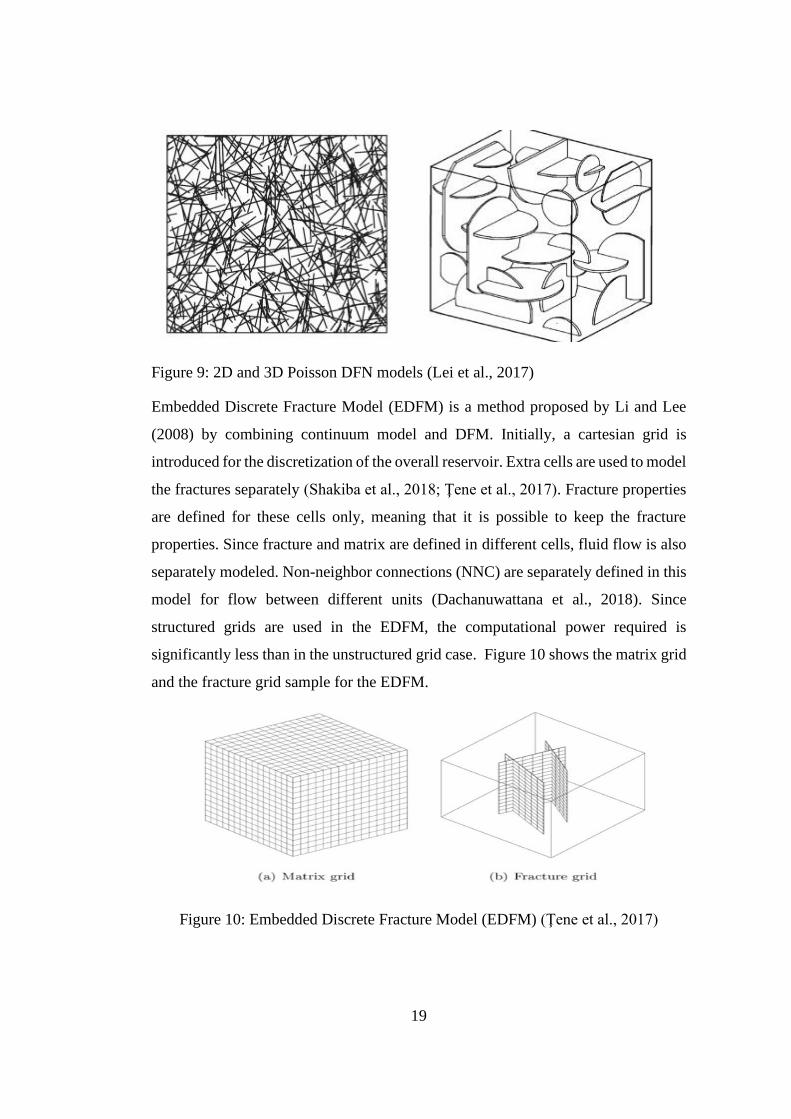
19
Figure 9: 2D and 3D Poisson DFN models (Lei et al., 2017)
Embedded Discrete Fracture Model (EDFM) is a method proposed by Li and Lee
(2008) by combining continuum model and DFM. Initially, a cartesian grid is
introduced for the discretization of the overall reservoir. Extra cells are used to model
the fractures separately (Shakiba et al., 2018; Ţene et al., 2017). Fracture properties
are defined for these cells only, meaning that it is possible to keep the fracture
properties. Since fracture and matrix are defined in different cells, fluid flow is also
separately modeled. Non-neighbor connections (NNC) are separately defined in this
model for flow between different units (Dachanuwattana et al., 2018). Since
structured grids are used in the EDFM, the computational power required is
significantly less than in the unstructured grid case. Figure 10 shows the matrix grid
and the fracture grid sample for the EDFM.
Figure 10: Embedded Discrete Fracture Model (EDFM) (Ţene et al., 2017)
20
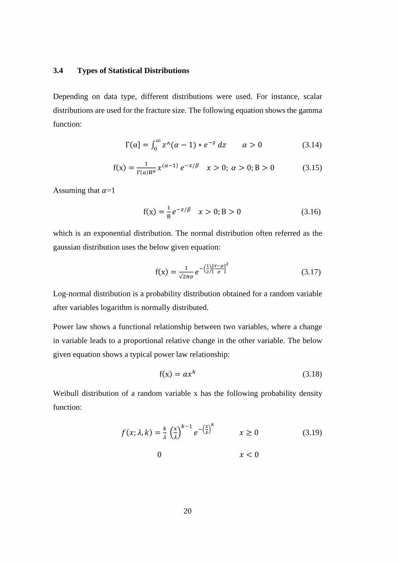
3.4 Types of Statistical Distributions
Depending on data type, different distributions were used. For instance, scalar
distributions are used for the fracture size. The following equation shows the gamma
function:
Γ(α] = ∫ 𝑧^(𝛼 − 1)∞
0∗ 𝑒−𝑧𝑑𝑧𝛼 > 0 (3.14)
f(x) =1
Γ(α)Βα 𝑥(𝛼−1)𝑒−𝑥/𝛽𝑥 > 0; 𝛼 > 0; Β > 0 (3.15)
Assuming that 𝛼=1
f(x) =1
Β𝑒−𝑥/𝛽𝑥 > 0; Β > 0 (3.16)
which is an exponential distribution. The normal distribution often referred as the
gaussian distribution uses the below given equation:
f(x) =1
√2𝜋𝜎𝑒−(
1
2)[
𝑥−𝜇
𝜎]2
(3.17)
Log-normal distribution is a probability distribution obtained for a random variable
after variables logarithm is normally distributed.
Power law shows a functional relationship between two variables, where a change
in variable leads to a proportional relative change in the other variable. The below
given equation shows a typical power law relationship:
f(x) = 𝑎𝑥𝑘 (3.18)
Weibull distribution of a random variable x has the following probability density
function:
𝑓(𝑥; 𝜆, 𝑘) =𝑘
𝜆(
𝑥
𝜆)𝑘−1
𝑒−(𝑥
𝜆)𝑘
𝑥 ≥ 0 (3.19)
0𝑥 < 0
21
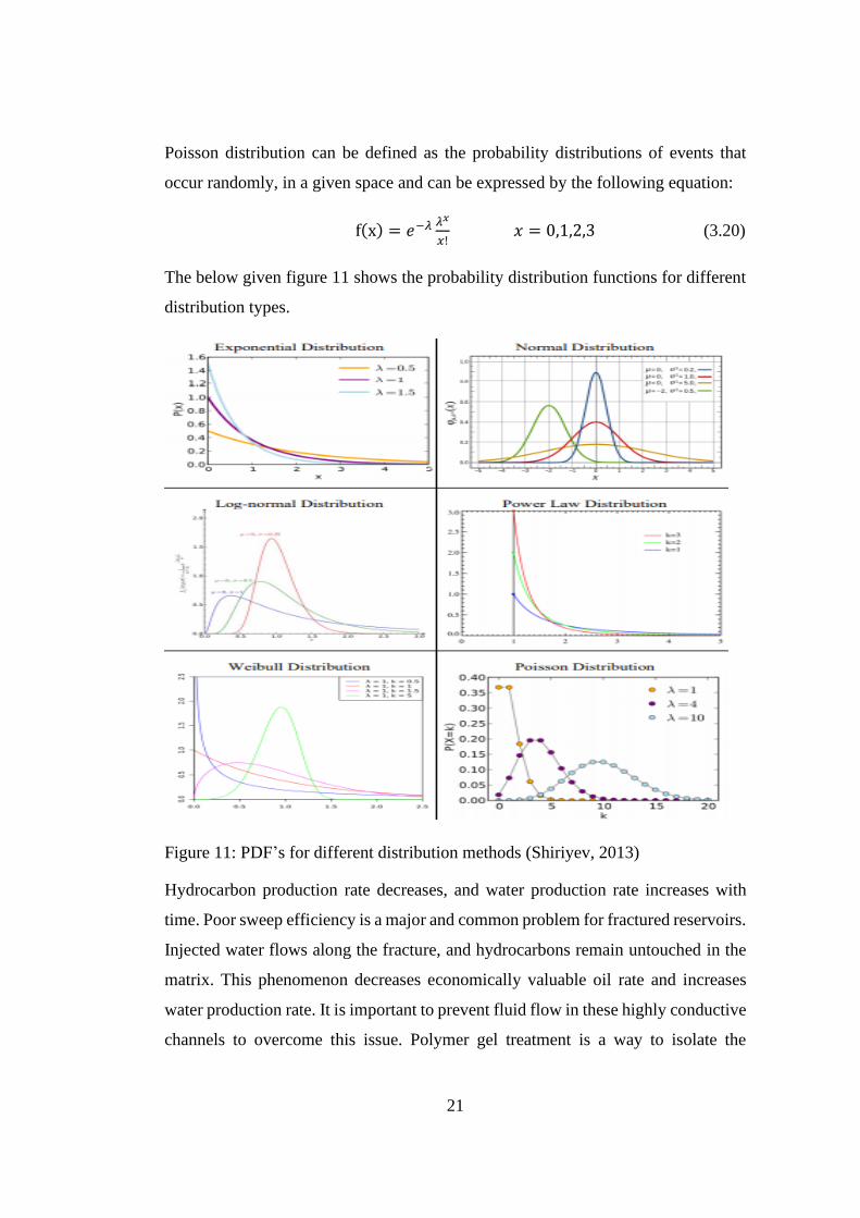
Poisson distribution can be defined as the probability distributions of events that
occur randomly, in a given space and can be expressed by the following equation:
f(x) = 𝑒−𝜆 𝜆𝑥
𝑥!𝑥 = 0,1,2,3 (3.20)
The below given figure 11 shows the probability distribution functions for different
distribution types.
Figure 11: PDF’s for different distribution methods (Shiriyev, 2013)
Hydrocarbon production rate decreases, and water production rate increases with
time. Poor sweep efficiency is a major and common problem for fractured reservoirs.
Injected water flows along the fracture, and hydrocarbons remain untouched in the
matrix. This phenomenon decreases economically valuable oil rate and increases
water production rate. It is important to prevent fluid flow in these highly conductive
channels to overcome this issue. Polymer gel treatment is a way to isolate the
22
fractures from the matrix blocks. In this way, it is possible to divert the injected water
into the poorly swept regions of the reservoir to increase the oil recovery. When
polymer gel is applied to a fracture, fracture permeability decreases significantly,
meaning that fractures are no longer highly permeable channels. Injected water
cannot flow along with the fractures and moves to the matrix and reaches the
production zones by pushing the hydrocarbons in the poorly swept regions (Brattekås
& Seright, 2018; Canbolat & Parlaktuna, 2019; Sydansk, 1988).
The efficiency of polymer gel treatment is proven by laboratory and field studies
(Herbas et al., 2004). Polymer gel treatment is generally conducted via preparing a
solution that contains the required chemical components. This solution is not the
final version of the gel, and it is called gellant. Under the temperature and pressure
conditions of the reservoir, the gellant becomes the gel after the gelation time passed.
Low resistance to the flow of the fracture and chemical structure of the gellant does
not permit the gellant to enter the small pores of the matrix, and gellant stays in the
large volume fracture aperture initially. However, in time a polymer concentration
difference between the fracture and matrix occurs. Due to this concentration
difference, the polymer tends to enter the rock matrix. Gel’s tendency to enter the
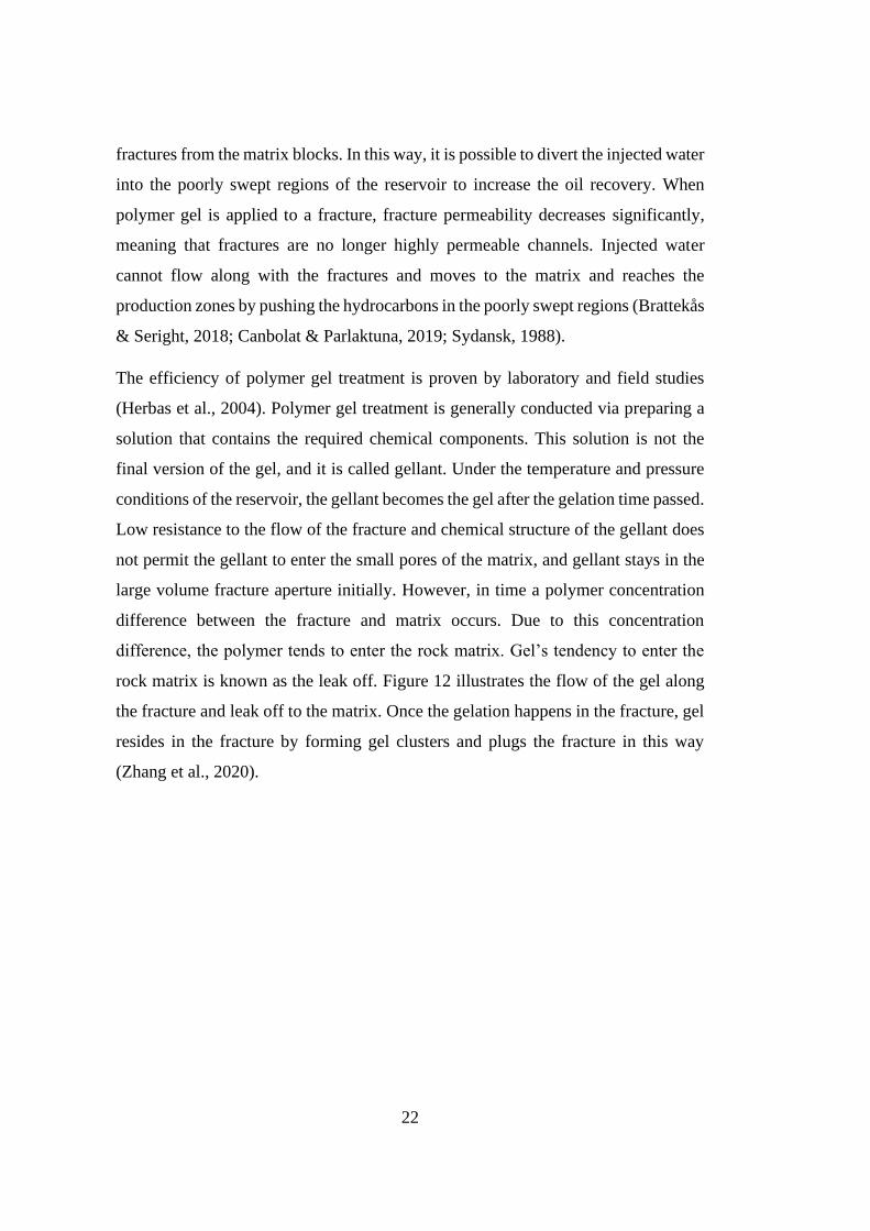
rock matrix is known as the leak off. Figure 12 illustrates the flow of the gel along
the fracture and leak off to the matrix. Once the gelation happens in the fracture, gel
resides in the fracture by forming gel clusters and plugs the fracture in this way
(Zhang et al., 2020).
23
Figure 12: Polymer gel treatment (Zhang et al., 2020)

25
CHAPTER 4
4 WATER FLOODING EXPERIMENTS
4.1 Core Plug Experiments
The water flooding experiments were conducted by using five different core plugs.
Three main cases, namely non-fractured, fractured, and polymer-gel treated core
plugs, were represented by these five different core plugs. Initially, two 2 PV water
was injected into all core samples. Polymer gel treatment was applied for the
artificially fractured core samples, and another 2 PV water was injected. A similar
approach was used for the non-fractured core plug to investigate the effects of
polymer gel treatment on the matrix. Table 1 summarizes core plugs.
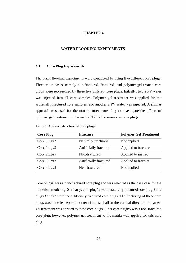
Table 1: General structure of core plugs
Core Plug Fracture Polymer Gel Treatment
Core Plug#2 Naturally fractured Not applied
Core Plug#3 Artificially fractured Applied to fracture
Core Plug#5 Non-fractured Applied to matrix
Core Plug#7 Artificially fractured Applied to fracture
Core Plug#8 Non-fractured Not applied
Core plug#8 was a non-fractured core plug and was selected as the base case for the
numerical modeling. Similarly, core plug#2 was a naturally fractured core plug. Core
plug#3 and#7 were the artificially fractured core plugs. The fracturing of these core
plugs was done by separating them into two half in the vertical direction. Polymer-
gel treatment was applied to these core plugs. Final core plug#5 was a non-fractured
core plug; however, polymer gel treatment to the matrix was applied for this core
plug.
26
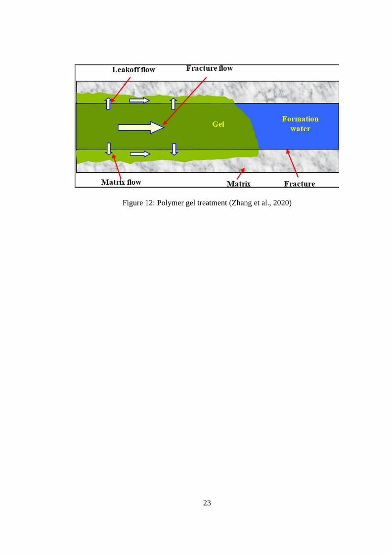
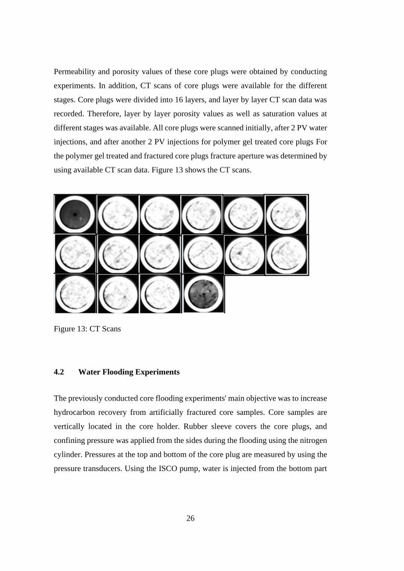
Permeability and porosity values of these core plugs were obtained by conducting
experiments. In addition, CT scans of core plugs were available for the different
stages. Core plugs were divided into 16 layers, and layer by layer CT scan data was
recorded. Therefore, layer by layer porosity values as well as saturation values at
different stages was available. All core plugs were scanned initially, after 2 PV water
injections, and after another 2 PV injections for polymer gel treated core plugs For
the polymer gel treated and fractured core plugs fracture aperture was determined by
using available CT scan data. Figure 13 shows the CT scans.
Figure 13: CT Scans
4.2 Water Flooding Experiments
The previously conducted core flooding experiments' main objective was to increase
hydrocarbon recovery from artificially fractured core samples. Core samples are
vertically located in the core holder. Rubber sleeve covers the core plugs, and
confining pressure was applied from the sides during the flooding using the nitrogen
cylinder. Pressures at the top and bottom of the core plug are measured by using the
pressure transducers. Using the ISCO pump, water is injected from the bottom part
27
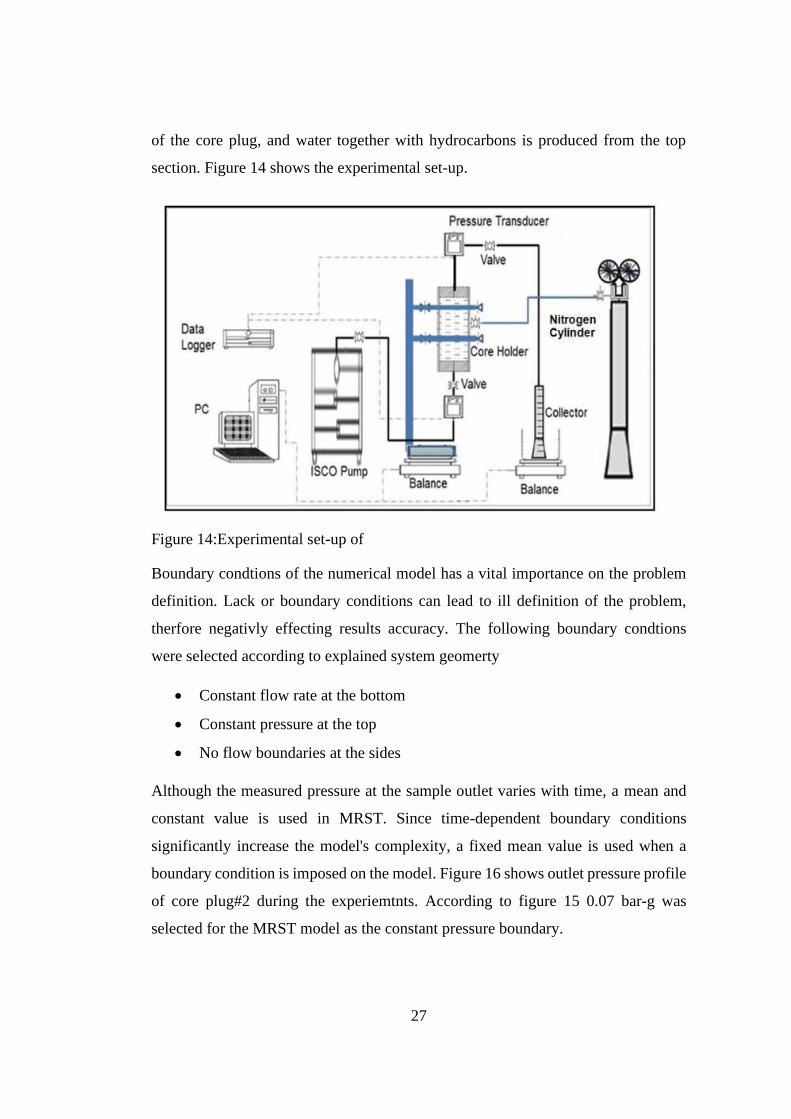
of the core plug, and water together with hydrocarbons is produced from the top
section. Figure 14 shows the experimental set-up.
Boundary condtions of the numerical model has a vital importance on the problem
definition. Lack or boundary conditions can lead to ill definition of the problem,
therfore negativly effecting results accuracy. The following boundary condtions
were selected according to explained system geomerty
• Constant flow rate at the bottom
• Constant pressure at the top
• No flow boundaries at the sides
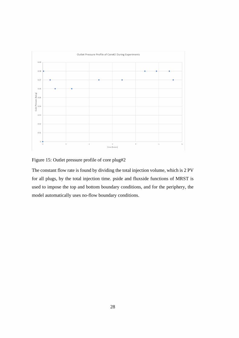
Although the measured pressure at the sample outlet varies with time, a mean and
constant value is used in MRST. Since time-dependent boundary conditions
significantly increase the model's complexity, a fixed mean value is used when a
boundary condition is imposed on the model. Figure 16 shows outlet pressure profile
of core plug#2 during the experiemtnts. According to figure 15 0.07 bar-g was
selected for the MRST model as the constant pressure boundary.
Figure 14:Experimental set-up of
28
Figure 15: Outlet pressure profile of core plug#2
The constant flow rate is found by dividing the total injection volume, which is 2 PV
for all plugs, by the total injection time. pside and fluxside functions of MRST is
used to impose the top and bottom boundary conditions, and for the periphery, the
model automatically uses no-flow boundary conditions.
29
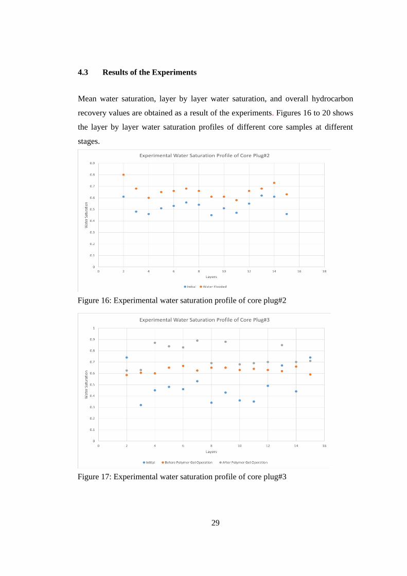
4.3 Results of the Experiments
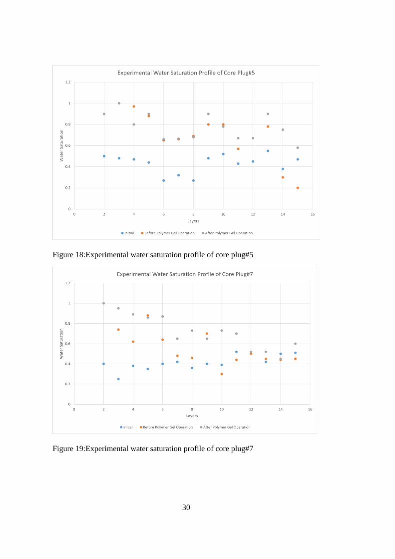
Mean water saturation, layer by layer water saturation, and overall hydrocarbon
recovery values are obtained as a result of the experiments. Figures 16 to 20 shows
the layer by layer water saturation profiles of different core samples at different
stages.
Figure 16: Experimental water saturation profile of core plug#2
Figure 17: Experimental water saturation profile of core plug#3
30
Figure 18:Experimental water saturation profile of core plug#5
Figure 19:Experimental water saturation profile of core plug#7
31
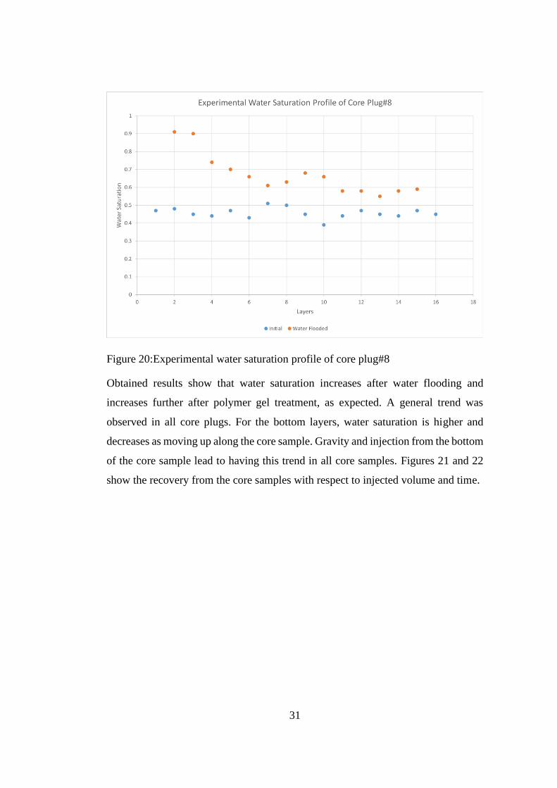
Figure 20:Experimental water saturation profile of core plug#8
Obtained results show that water saturation increases after water flooding and
increases further after polymer gel treatment, as expected. A general trend was
observed in all core plugs. For the bottom layers, water saturation is higher and
decreases as moving up along the core sample. Gravity and injection from the bottom
of the core sample lead to having this trend in all core samples. Figures 21 and 22
show the recovery from the core samples with respect to injected volume and time.
32
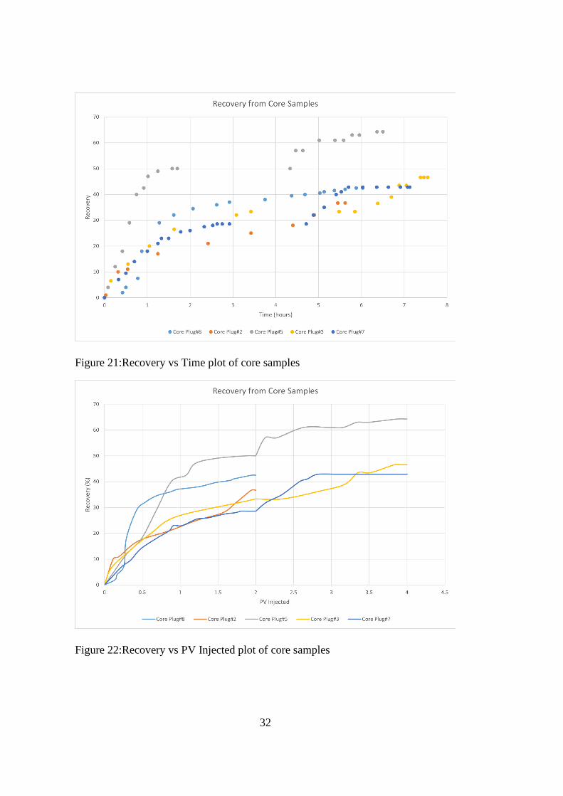
Figure 21:Recovery vs Time plot of core samples
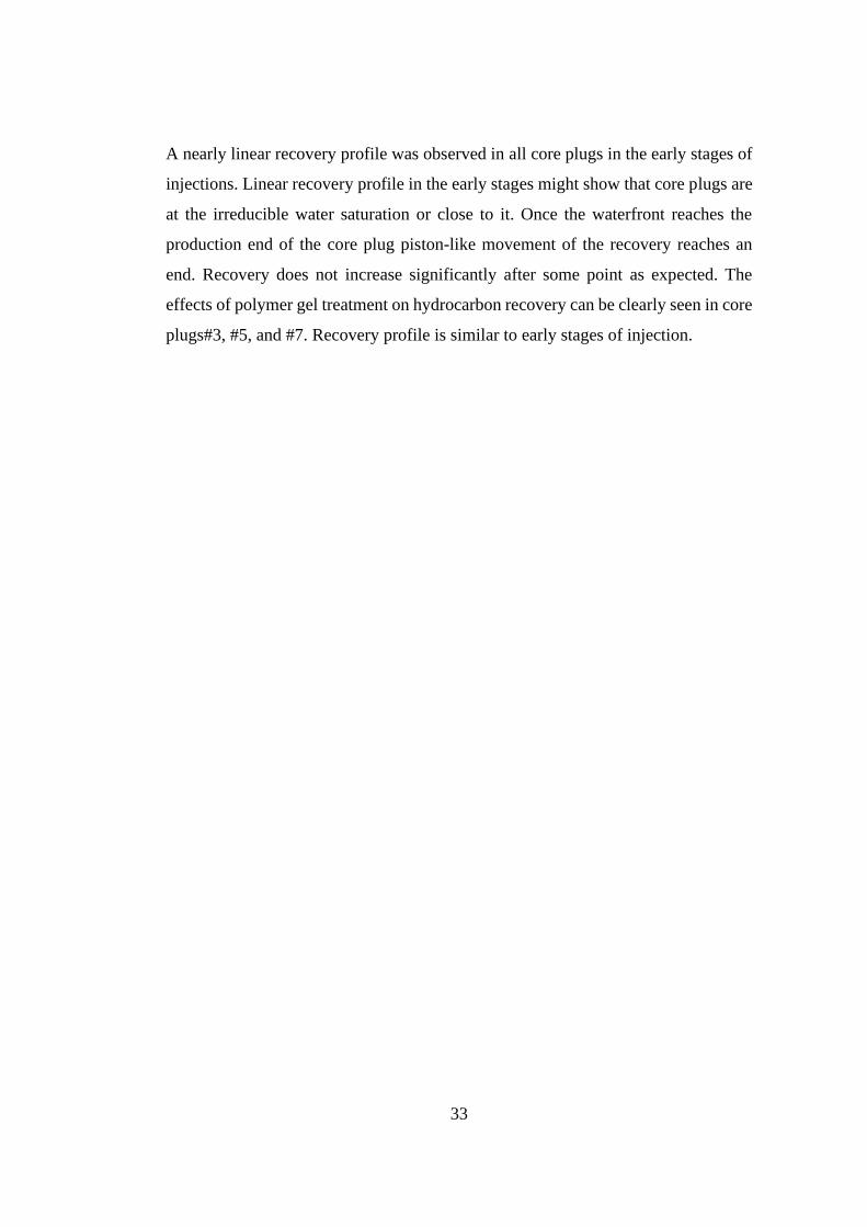
Figure 22:Recovery vs PV Injected plot of core samples
33
A nearly linear recovery profile was observed in all core plugs in the early stages of
injections. Linear recovery profile in the early stages might show that core plugs are
at the irreducible water saturation or close to it. Once the waterfront reaches the
production end of the core plug piston-like movement of the recovery reaches an
end. Recovery does not increase significantly after some point as expected. The
effects of polymer gel treatment on hydrocarbon recovery can be clearly seen in core
plugs#3, #5, and #7. Recovery profile is similar to early stages of injection.

35
CHAPTER 5
5 STATEMENT OF PROBLEM
The main objective of this thesis is numerically model water flooding experiments
in artificially fractured and gel-treated core plugs. A numerical model of the core
plugs was created using MRST, and validation of the MRST model is done using the
standard Buckley-Leveret method. Once the model is validated, non-fractured,
fractured, and polymer gel treated core plugs were modeled. EDFM was used to
introduce fractures into the model. Water injection into these core plug models was
simulated by using MRST, and obtained results were compared with the
experimental results. The effects of the polymer gel treatment of matrix and fractures
on the oil recovery were investigated. 3D fluid saturation profiles of the core samples
during the injection as well as final oil recovery vs. time plots are obtained with
MRST. Obtained oil recovery and mean water saturation values are compared with
the results of the experiments. Moreover, additional simulations were completed to
investigate how oil recovery changes with the fracture permeability and aperture.

37
CHAPTER 6
6 NUMERICAL MODELLING
6.1 MATLAB Reservoir Simulation Toolbox (MRST)
MRST is an open-source code library for MATLAB that is introduced and developed
mainly by the SINTEF Technology and Society, a Norwegian research institute.
MRST can be used to create reservoir models and to simulate those models for
different cases. MRST consists of various modules from the basic reservoir
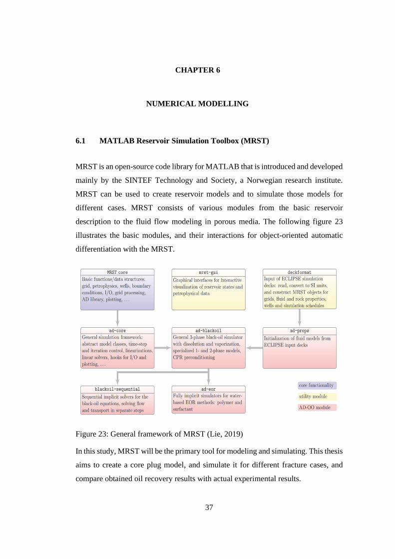
description to the fluid flow modeling in porous media. The following figure 23
illustrates the basic modules, and their interactions for object-oriented automatic
differentiation with the MRST.
Figure 23: General framework of MRST (Lie, 2019)
In this study, MRST will be the primary tool for modeling and simulating. This thesis
aims to create a core plug model, and simulate it for different fracture cases, and
compare obtained oil recovery results with actual experimental results.
38
6.2 MRST Tools
6.2.1 Automatic Differentiation (AD)
The main idea of automatic differentiation (AD) is implementing basic operations
in a numerical model. AD uses fundamental derivative rules and evaluates and
stores the function and its derivative simultaneously.
In MRST, the object-oriented automatic differentiation (AD-OO) framework is
introduced. In this framework, implementation of the fundamental components like
physical models, discrete operators, time-stepping are separated. This enables,
implementation of new models that can work with the existing solvers in the
MRST. This procedure is suitable for complex features like multi-phase flow, as it
makes simulations less complex.
Below given example provides a better explanation of the AD in MRST.
𝑓(𝑥, 𝑦) = 10𝑥 − 2𝑦 − 25
Derivative of the f function is stored as
∇𝑓(𝑥, 𝑦) = [10,−2] = [𝜕𝑓
𝜕𝑥,𝜕𝑓
𝜕𝑦]
Setting x= 5 and y=2 automatic differentiation of the f function is as following
𝑣𝑎𝑙 = 21
𝑗𝑎𝑐 = {[10][−2]}
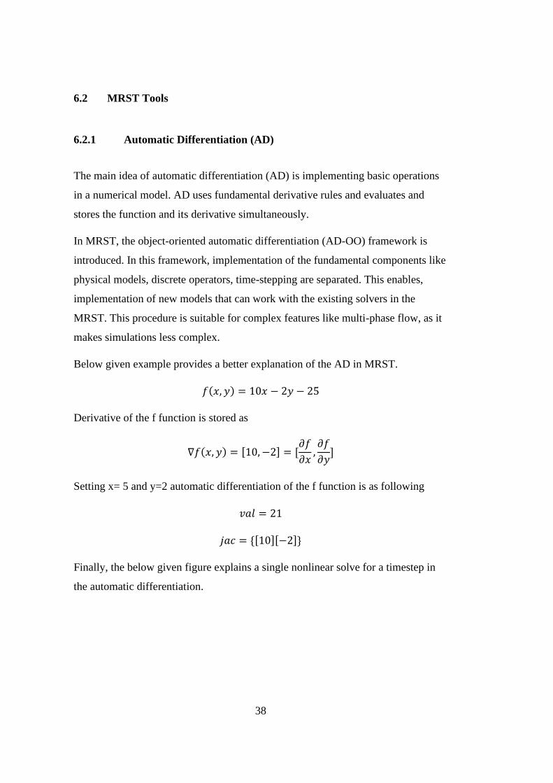
Finally, the below given figure explains a single nonlinear solve for a timestep in
the automatic differentiation.
39
Figure 24: Mini-step solution procedure of AD (Lie, 2019)
6.2.2 Two Point Flux Approximation
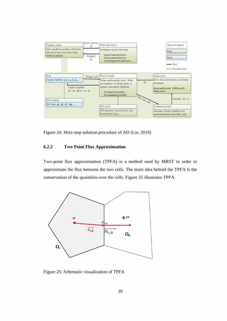
Two-point flux approximation (TPFA) is a method used by MRST in order to
approximate the flux between the two cells. The main idea behind the TPFA is the
conservation of the quantities over the cells. Figure 25 illustrates TPFA.
Figure 25: Schematic visualization of TPFA
40
Simplified flow equation for a single phase is given below
∇𝑣 = 𝑞 (6.1)
𝑣 = −𝐾∇𝑝 (6.2)
The main goal here is the discretization of equation … for a finite-volume scheme.
The integral form of this equation for a single cell
∫ 𝑣⃗⃗⃗ . 𝑛⃗⃗ ⃗𝑑𝑠0
𝜕𝛺𝑖= ∫ 𝑞
0
𝛺𝑖𝑑𝑥 (6.3)
This equation is a simpler form of the conservation of the material over boundaries
which is given below
𝜕
𝜕𝑡∫ 𝜌𝜙
0
𝛺𝑑𝑥 + ∫ 𝜌𝑣⃗⃗⃗ . 𝑛⃗⃗ ⃗𝑑𝑠
0
𝜕𝛺= ∫ 𝜌𝑞
0
𝛺𝑑𝑥 (6.4)
Since density and porosity does not depend on the time therefore, they do not have
an effect on the discretization and eliminated. Computing the flux for each face of a
cell by using the Darcy’s law leads to
𝑣𝑖,𝑘 = ∫ 𝑣⃗⃗⃗ . 𝑛⃗⃗ ⃗𝑑𝑠0
𝜏𝑖,𝑘 (6.5)
𝜏𝑖,𝑘 is the half faces for grid cell Ωi . By using the mid-point rule, approximation of
the integral over the cells face and expressing the flux by using Darcy’s law leads to
𝑣𝑖,𝑘 = −𝐴𝑖,𝑘(𝐾∇𝑝)(𝑥𝑖,𝑘)⃗⃗ ⃗⃗ ⃗⃗ ⃗⃗ ⃗. 𝑛𝑖,𝑘⃗⃗ ⃗⃗ ⃗⃗ ⃗⃗ (6.6)
Centroids of the half faces are denoted with the 𝑥⃗⃗⃗ . Next step is the one-side finite
difference method to shows the pressure change between the face centroid and a
random point in cell. A linear pressure profile is needed and assumed since cell
averaged pressure inside the cell is available in finite-volume method. A linear
pressure profile inside a cell means that pressure at the cell center is equal to the
average pressure and the following equation is obtained
41
𝑣𝑖,𝑘 = −𝐴𝑖,𝑘𝐾𝑖(𝑝𝑖−𝜋𝑖,𝑘)𝑐𝑖,𝑘⃗⃗⃗⃗ ⃗⃗ ⃗
|𝑐𝑖,𝑘⃗⃗⃗⃗ ⃗⃗ ⃗|2 𝑛𝑖,𝑘⃗⃗ ⃗⃗ ⃗⃗ ⃗⃗ = Ti,k(𝑝𝑖 − 𝜋𝑖,𝑘) (6.7)
One-sided transmissibilities are introduced with T which is related with a one cell.
This transmissibility provides a flux relationship between a face centroid and cell,
Therefore, they are associated with a half face meaning that it is possible to refer
them as half-transmissibilities. Finally, imposing the face pressure and flux
continuity and eliminating interface pressure lead to
𝑣𝑖,𝑘 = [Ti,k−1 + Tk,i
−1]−1
(𝑝𝑖 − 𝑝𝑘) = 𝑇𝑖𝑘(𝑝𝑖 − 𝑝𝑘) (6.8)
Which is the two-point flux approximation structure that is used in MRST. In
summary TPFA, uses cell average pressures 𝑝𝑖𝑎𝑛𝑑𝑝𝑘 to approximate the fluid flux
between Ωi and Ωk . Figure 16 illustrates the TPFA.
6.3 Modelling the Non-Fractured/Non-Gel Treated Core Plug#8
It is required to convert the physical core plug into a set of points that describes the
geometry of the core plug. This can be done by gridding. Type of grid selection is
crucial, and grid type determines functions that can be used, heterogeneities need to
be shown, etc. Although unstructured grids are more successful in representing
geometry, they cause more errors in discretization. Therefore, in this study Cartesian
grid is used to define and model the medium geometry.
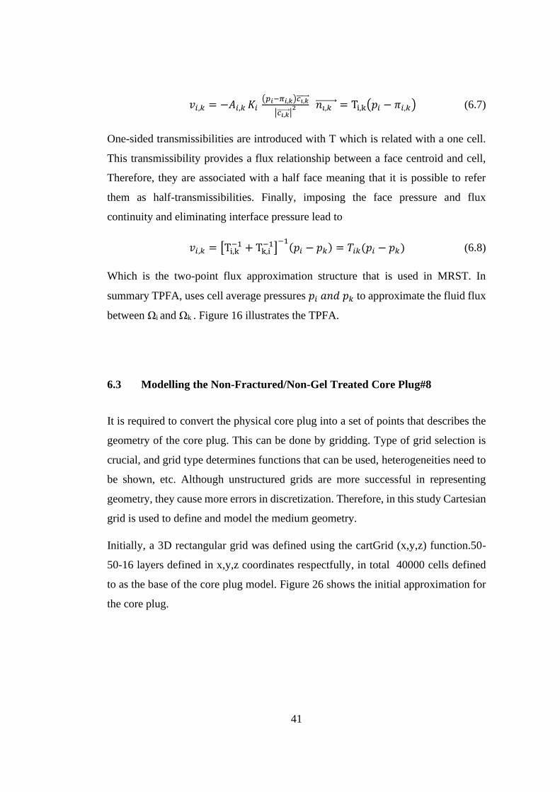
Initially, a 3D rectangular grid was defined using the cartGrid (x,y,z) function.50-
50-16 layers defined in x,y,z coordinates respectfully, in total 40000 cells defined
to as the base of the core plug model. Figure 26 shows the initial approximation for
the core plug.
42
Figure 26: Base grid structure of core plug#8
Removal of edge cells to obtain a cylindrical shape is the next step. As the core plugs
are all cylindrically shaped, and the based model is a rectangular prism, the radius of
the core plug (1.85 cm) is defined in the center of the base model, and the cells whose
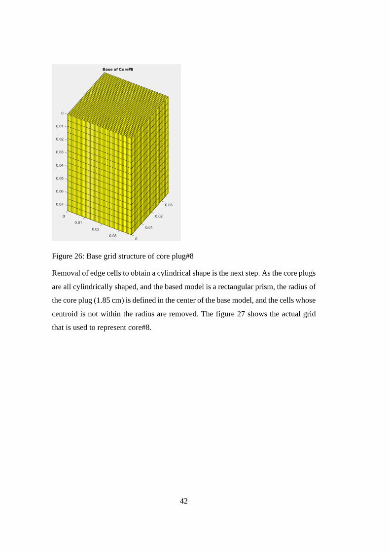
centroid is not within the radius are removed. The figure 27 shows the actual grid
that is used to represent core#8.
43
Figure 27: Grid structure of core plug#8
After removing the edges, the total number of cells in the grid reduced to 31616. In
each layer, there are 1976 cells, and there are 16 layers in total. 16 layers in z
direction selected according to the CT scans.
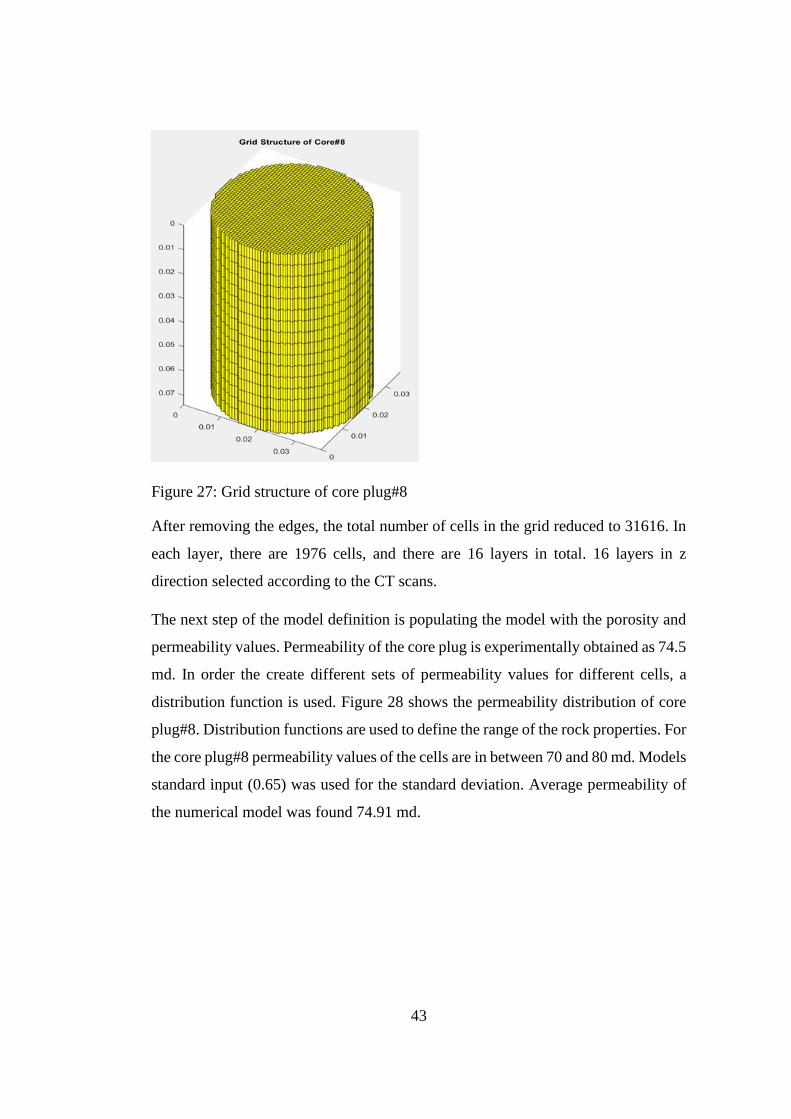
The next step of the model definition is populating the model with the porosity and
permeability values. Permeability of the core plug is experimentally obtained as 74.5
md. In order the create different sets of permeability values for different cells, a
distribution function is used. Figure 28 shows the permeability distribution of core
plug#8. Distribution functions are used to define the range of the rock properties. For
the core plug#8 permeability values of the cells are in between 70 and 80 md. Models
standard input (0.65) was used for the standard deviation. Average permeability of
the numerical model was found 74.91 md.
44
Figure 28: Permeability distribution of core plug#8
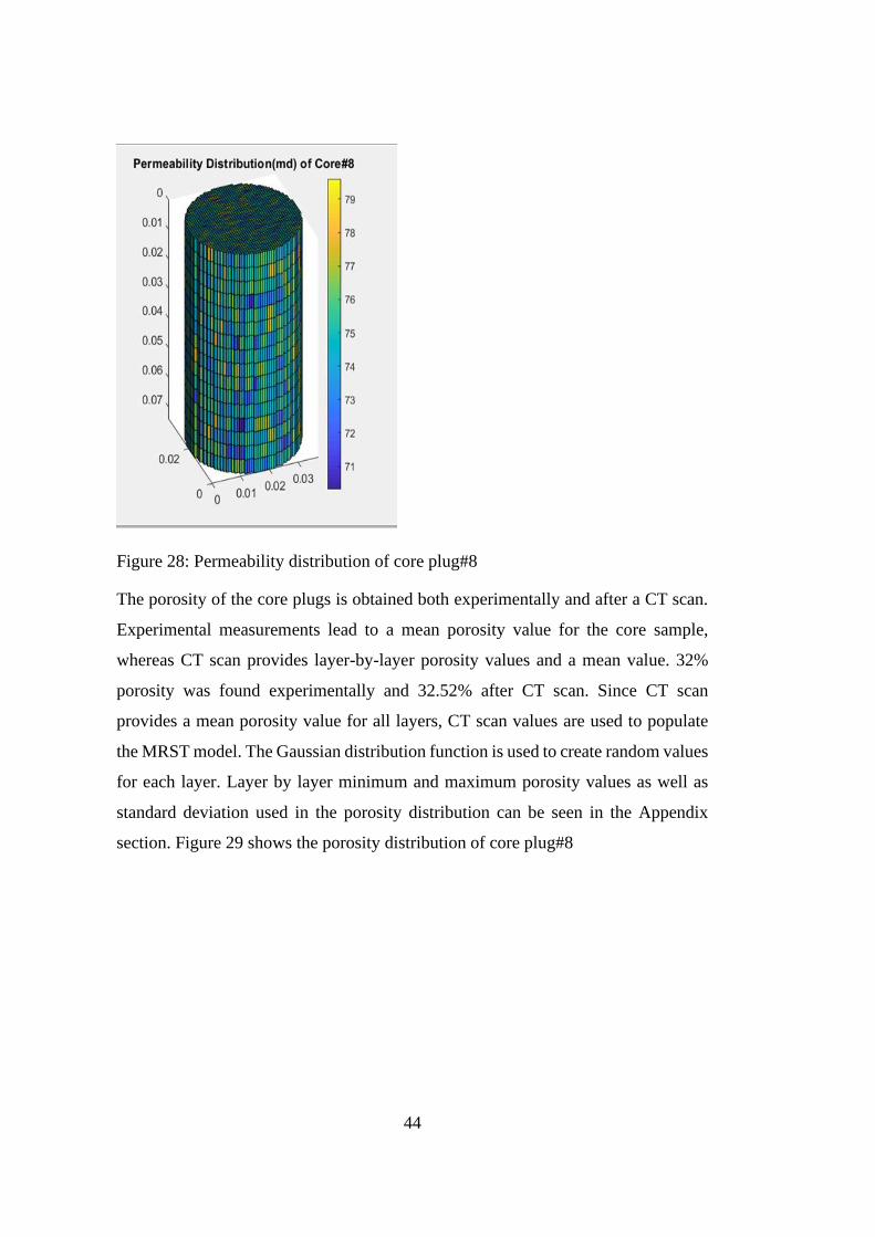
The porosity of the core plugs is obtained both experimentally and after a CT scan.
Experimental measurements lead to a mean porosity value for the core sample,
whereas CT scan provides layer-by-layer porosity values and a mean value. 32%
porosity was found experimentally and 32.52% after CT scan. Since CT scan
provides a mean porosity value for all layers, CT scan values are used to populate
the MRST model. The Gaussian distribution function is used to create random values
for each layer. Layer by layer minimum and maximum porosity values as well as
standard deviation used in the porosity distribution can be seen in the Appendix
section. Figure 29 shows the porosity distribution of core plug#8
45
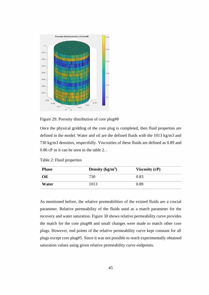
Figure 29: Porosity distribution of core plug#8
Once the physical gridding of the core plug is completed, then fluid properties are
defined in the model. Water and oil are the defined fluids with the 1013 kg/m3 and
730 kg/m3 densities, respectfully. Viscosities of these fluids are defined as 0.89 and
0.86 cP as it can be seen in the table 2. .
Table 2: Fluid properties
Phase Density (kg/m3) Viscosity (cP)
Oil 730 0.83
Water 1013 0.89
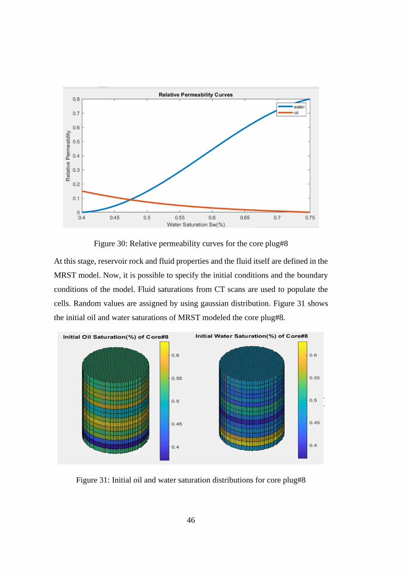
As mentioned before, the relative permeabilities of the existed fluids are a crucial
parameter. Relative permeability of the fluids used as a match parameter for the
recovery and water saturation. Figure 30 shows relative permeability curve provides
the match for the core plug#8 and small changes were made to match other core
plugs. However, end points of the relative permeability curve kept constant for all
plugs except core plug#5. Since it was not possible to reach experimentally obtained
saturation values using given relative permeability curve endpoints.
46
Figure 30: Relative permeability curves for the core plug#8
At this stage, reservoir rock and fluid properties and the fluid itself are defined in the
MRST model. Now, it is possible to specify the initial conditions and the boundary
conditions of the model. Fluid saturations from CT scans are used to populate the
cells. Random values are assigned by using gaussian distribution. Figure 31 shows
the initial oil and water saturations of MRST modeled the core plug#8.
Figure 31: Initial oil and water saturation distributions for core plug#8
47
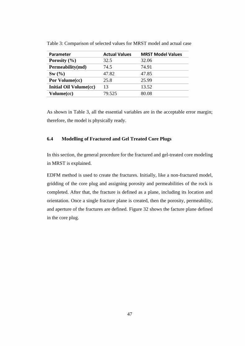
Table 3: Comparison of selected values for MRST model and actual case
Parameter Actual Values MRST Model Values Porosity (%) 32.5 32.06
Permeability(md) 74.5 74.91
Sw (%) 47.82 47.85
Por Volume(cc) 25.8 25.99
Initial Oil Volume(cc) 13 13.52
Volume(cc) 79.525 80.08
As shown in Table 3, all the essential variables are in the acceptable error margin;
therefore, the model is physically ready.
6.4 Modelling of Fractured and Gel Treated Core Plugs
In this section, the general procedure for the fractured and gel-treated core modeling
in MRST is explained.
EDFM method is used to create the fractures. Initially, like a non-fractured model,
gridding of the core plug and assigning porosity and permeabilities of the rock is
completed. After that, the fracture is defined as a plane, including its location and
orientation. Once a single fracture plane is created, then the porosity, permeability,
and aperture of the fractures are defined. Figure 32 shows the facture plane defined
in the core plug.
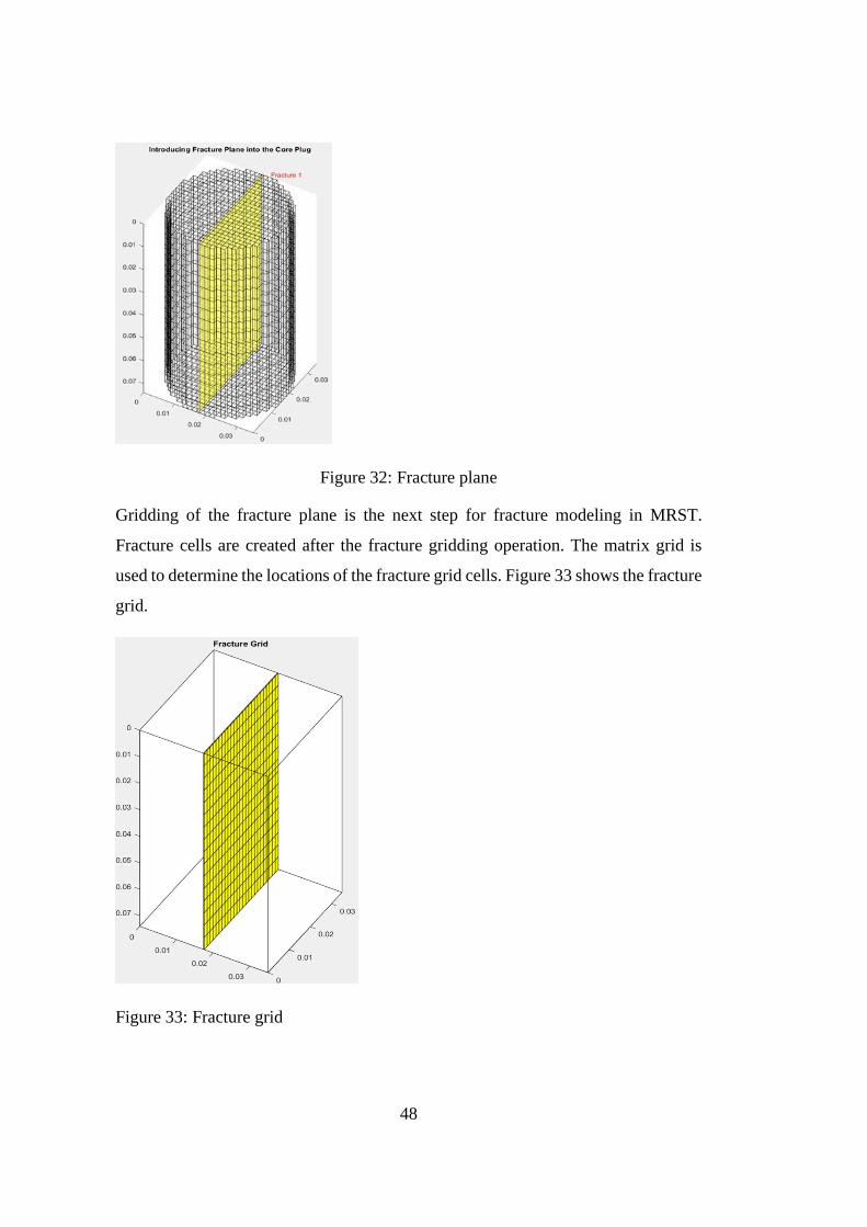
48
Figure 32: Fracture plane
Gridding of the fracture plane is the next step for fracture modeling in MRST.
Fracture cells are created after the fracture gridding operation. The matrix grid is
used to determine the locations of the fracture grid cells. Figure 33 shows the fracture
grid.
Figure 33: Fracture grid
49
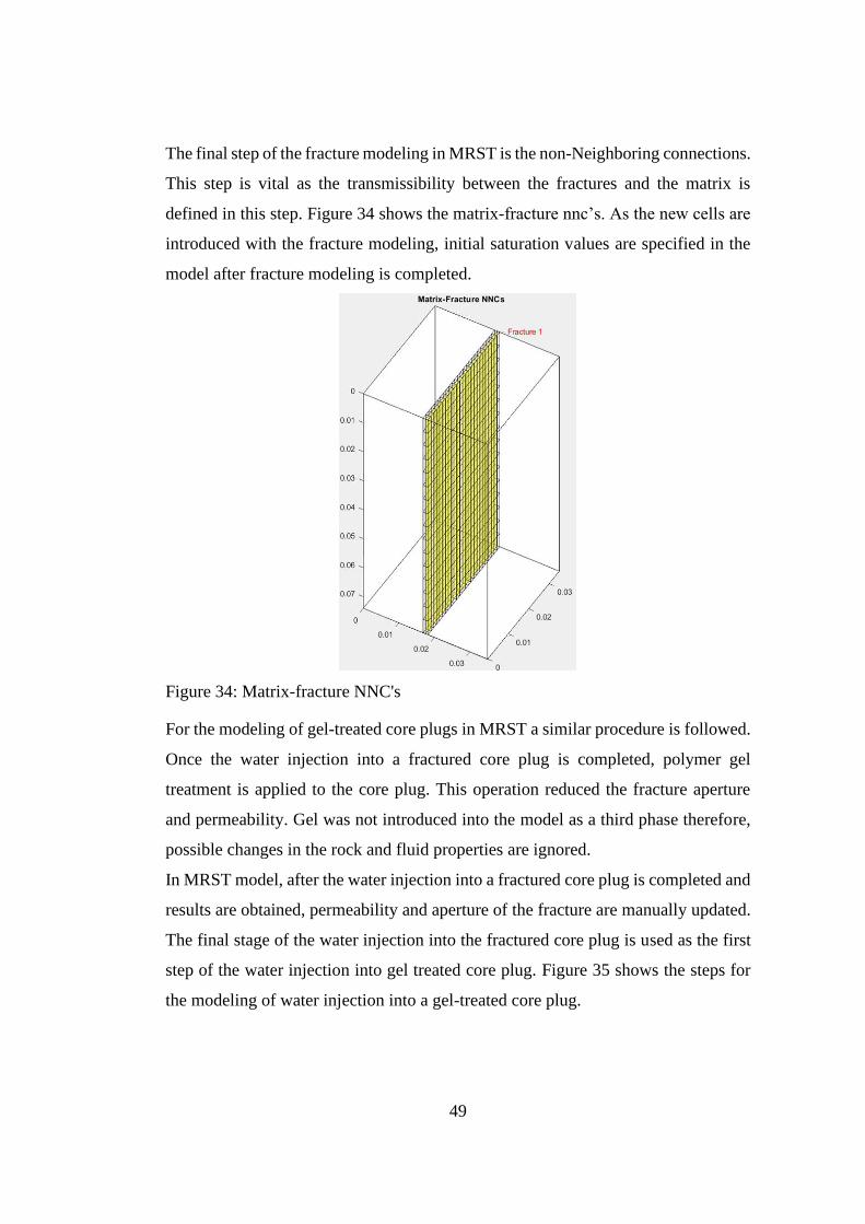
The final step of the fracture modeling in MRST is the non-Neighboring connections.
This step is vital as the transmissibility between the fractures and the matrix is
defined in this step. Figure 34 shows the matrix-fracture nnc’s. As the new cells are
introduced with the fracture modeling, initial saturation values are specified in the
model after fracture modeling is completed.
Figure 34: Matrix-fracture NNC's
For the modeling of gel-treated core plugs in MRST a similar procedure is followed.
Once the water injection into a fractured core plug is completed, polymer gel
treatment is applied to the core plug. This operation reduced the fracture aperture
and permeability. Gel was not introduced into the model as a third phase therefore,
possible changes in the rock and fluid properties are ignored.
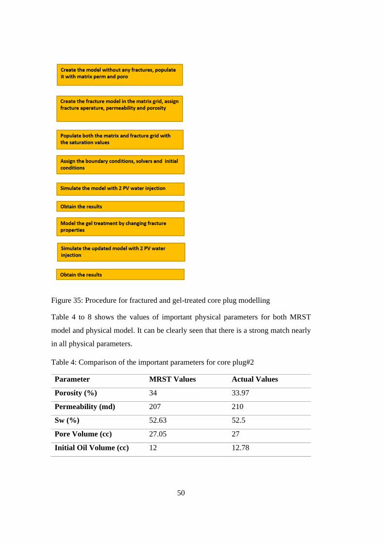
In MRST model, after the water injection into a fractured core plug is completed and
results are obtained, permeability and aperture of the fracture are manually updated.
The final stage of the water injection into the fractured core plug is used as the first
step of the water injection into gel treated core plug. Figure 35 shows the steps for
the modeling of water injection into a gel-treated core plug.
50
Figure 35: Procedure for fractured and gel-treated core plug modelling
Table 4 to 8 shows the values of important physical parameters for both MRST
model and physical model. It can be clearly seen that there is a strong match nearly
in all physical parameters.
Table 4: Comparison of the important parameters for core plug#2
Parameter MRST Values Actual Values
Porosity (%) 34 33.97
Permeability (md) 207 210
Sw (%) 52.63 52.5
Pore Volume (cc) 27.05 27
Initial Oil Volume (cc) 12 12.78
51
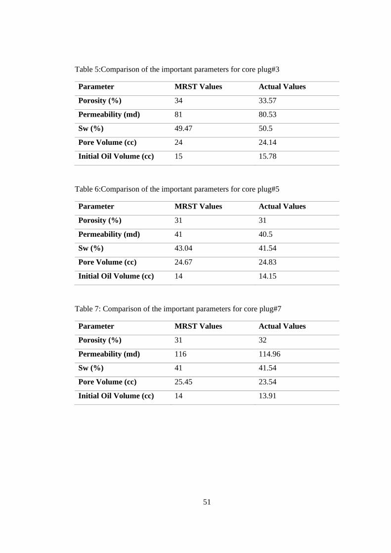
Table 5:Comparison of the important parameters for core plug#3
Parameter MRST Values Actual Values
Porosity (%) 34 33.57
Permeability (md) 81 80.53
Sw (%) 49.47 50.5
Pore Volume (cc) 24 24.14
Initial Oil Volume (cc) 15 15.78
Table 6:Comparison of the important parameters for core plug#5
Parameter MRST Values Actual Values
Porosity (%) 31 31
Permeability (md) 41 40.5
Sw (%) 43.04 41.54
Pore Volume (cc) 24.67 24.83
Initial Oil Volume (cc) 14 14.15
Table 7: Comparison of the important parameters for core plug#7
Parameter MRST Values Actual Values
Porosity (%) 31 32
Permeability (md) 116 114.96
Sw (%) 41 41.54
Pore Volume (cc) 25.45 23.54
Initial Oil Volume (cc) 14 13.91
52
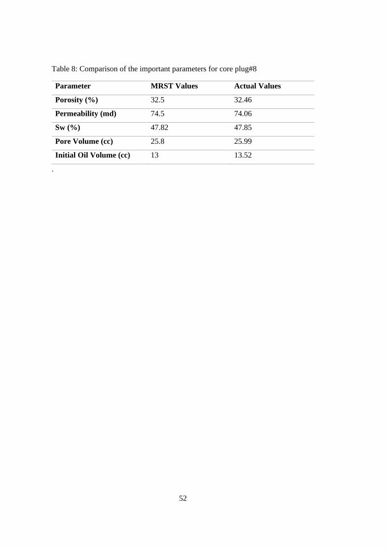
Table 8: Comparison of the important parameters for core plug#8
Parameter MRST Values Actual Values
Porosity (%) 32.5 32.46
Permeability (md) 74.5 74.06
Sw (%) 47.82 47.85
Pore Volume (cc) 25.8 25.99
Initial Oil Volume (cc) 13 13.52
.
53
CHAPTER 7
7 VALIDATION OF MODEL
7.1 General Buckley-Leveret Solution
Buckley-Leveret solution is an analytical verification tool that is used in this thesis
to validate the model. Buckley-Leveret solution determines the distance of the high-
water saturation at any time for the water flooding applications. The main
assumptions of the Buckley-Leveret (Buckley & Leverett, 1942) solution is listed
below
• Water injection to an oil reservoir and flow is linear and horizontal
• Incompressible and immiscible fluids
• Neglected gravity
• Neglected capillary pressure effects
Darcy equation for the multiphase flow with the above listed assumptions is given
below for both oil and water phases.
𝑞𝑤 =𝑘𝑘𝑟𝑤𝐴
𝜇𝑤
𝜕𝑃
𝜕𝑥 (7.1)
𝑞𝑜 =𝑘𝑘𝑟𝑜𝐴
𝜇𝑜
𝜕𝑃
𝜕𝑥 (7.2)
Defining the fractional flow for water as following
𝑓𝑤 =𝑞𝑤
𝑞𝑜+𝑞𝑤 (7.3)
Plugging qo and qw and canceling out common terms leads to
𝑓𝑤 =
𝑘𝑟𝑤𝜇𝑤
𝑘𝑟𝑜𝜇𝑜
+𝑘𝑟𝑤𝜇𝑤
(7.4)
54
𝑓𝑤 =1
𝑘𝑟𝑜𝜇𝑤𝑘𝑟𝑤𝜇𝑜
+1 (7.5)
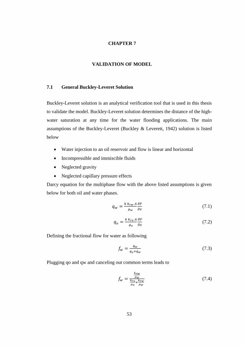
A standard fractional flow plot is given below in figure 36.
Figure 36: Typical fractional flow curve
For a non-horizontal system gravity effect needs to be included the following form
of the fractional flow equation includes the gravity effect.
𝑓𝑤 =1+
𝑘𝑘𝑟𝑜𝐴
𝑞𝜇𝑜(𝜕𝑃𝑐𝑜𝑤
𝜕𝑥−∆𝜌𝑔𝑠𝑖𝑛𝛼)
1+𝑘𝑟𝑜𝜇𝑤𝑘𝑟𝑤𝜇𝑜
(7.6)
Mass balance of the frontal displacement for the water phase in general form can be
expressed as given below
[(𝑞𝑤𝜌𝑤)𝑥 − (𝑞𝑤𝜌𝑤)𝑥+∆𝑥]∆𝑡 = 𝐴∆𝑥𝜙[(𝑆𝑤𝜌𝑤)𝑡+∆𝑡 − (𝑆𝑤𝜌𝑤)𝑡] (7.7)
Neglecting the compressibility and converting this equation to continuity equation
by ∆𝑥, ∆𝑡 → 0𝑎𝑛𝑑𝑞𝑤 = 𝑓𝑤 ∗ 𝑞
55
−𝜕𝑓𝑤
𝜕𝑥=
𝐴𝜙
𝑞
𝜕𝑆𝑤
𝜕𝑡 (7.8)
since fractional flow is a function of water saturation
−𝑑𝑓𝑤
𝑑𝑆𝑤
𝜕𝑆𝑤
𝜕𝑥=
𝐴𝜙
𝑞
𝜕𝑆𝑤
𝜕𝑡 (7.9)
Which is known as the Buckley-Leveret equation. It is possible to modify equation
6.9 and derive the frontal advance equation for the water injection. Since water
saturation along the core sample depends on the location and the time
𝑑𝑆𝑤 =𝜕𝑆𝑤
𝜕𝑥𝑑𝑥 +
𝜕𝑆𝑤
𝜕𝑡𝑑𝑡 (7.10)
Assuming that water saturation is constant at the front
0 =𝜕𝑆𝑤
𝜕𝑥𝑑𝑥 +
𝜕𝑆𝑤
𝜕𝑡𝑑𝑡 (7.11)
Plugging equation 6.11 into the Buckley-Leveret equation and integration over time
leads to the following equation
𝑥𝑓 =𝑞𝑡
𝐴𝜙(𝑑𝑓𝑤
𝑑𝑆𝑤)𝑓 (7.12)
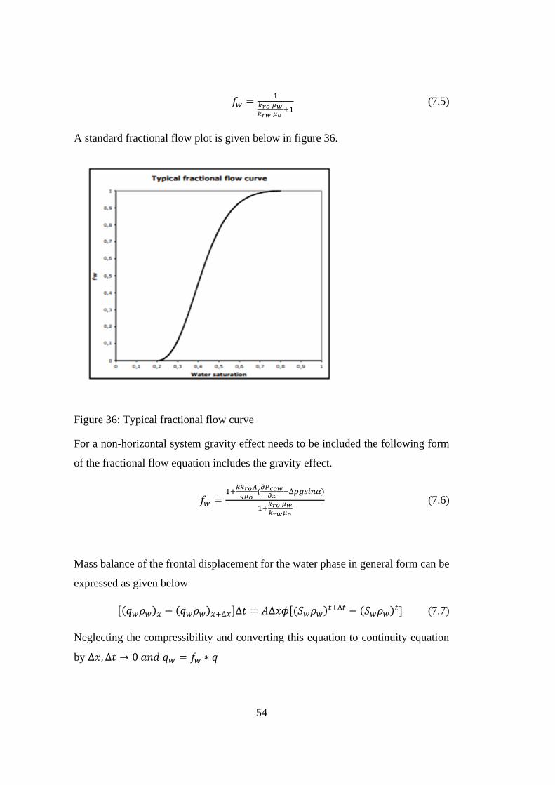
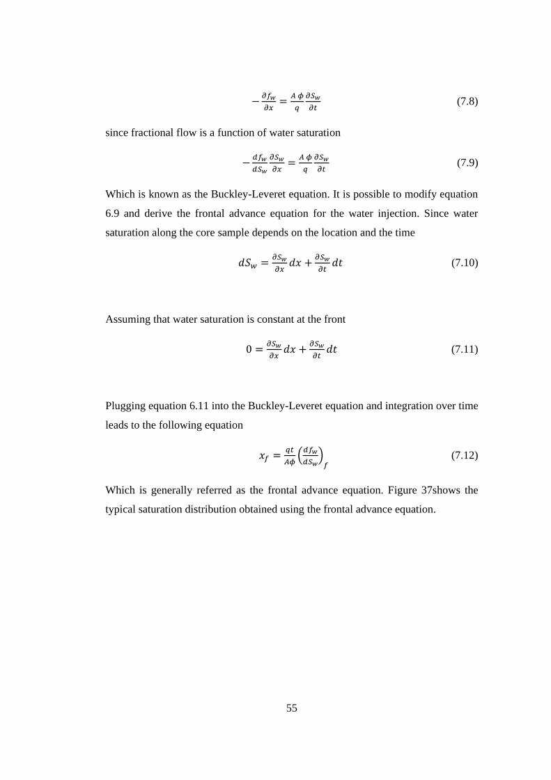
Which is generally referred as the frontal advance equation. Figure 37shows the
typical saturation distribution obtained using the frontal advance equation.
56
Figure 37: Typical frontal advance profile for waterflooding
7.2 Model Validation
A new simple grid structure was designed and created for the validation of the
solvers, models and assumptions used in the MRST model solution. A grid with the
following properties is created
• The reservoir is 1 meter wide, 1 meter thick and 100 meter long and 100%
oil saturated
• 1 cell used to represent wide and thickness of the model and 4000 cells used
to represent length
• Rock porosity and permeability is constant and assumed as 0.2 and 100 md
respectively
• Continuous water injection from the injection end (left) of the model
• Production occurs only in the production end (right) of the reservoir and other
boundaries are assumed as no flow boundaries
• Total injection volume of water is 0.5 pore volume and total injection time is
1000 seconds
• 1013 and 730 kg/m3 densities with 0.89 and 0.86 cp viscosities used for water
and oil phases respectively
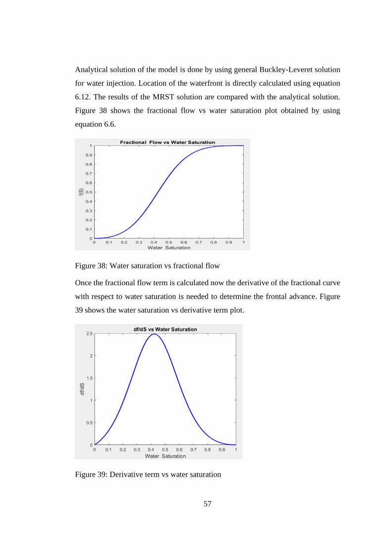
57
Analytical solution of the model is done by using general Buckley-Leveret solution
for water injection. Location of the waterfront is directly calculated using equation
6.12. The results of the MRST solution are compared with the analytical solution.
Figure 38 shows the fractional flow vs water saturation plot obtained by using
equation 6.6.
Figure 38: Water saturation vs fractional flow
Once the fractional flow term is calculated now the derivative of the fractional curve
with respect to water saturation is needed to determine the frontal advance. Figure
39 shows the water saturation vs derivative term plot.
Figure 39: Derivative term vs water saturation
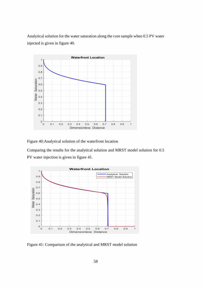
58
Analytical solution for the water saturation along the core sample when 0.5 PV water
injected is given in figure 40.
Figure 40:Analytical solution of the waterfront location
Comparing the results for the analytical solution and MRST model solution for 0.5
PV water injection is given in figure 41.
Figure 41: Comparison of the analytical and MRST model solution
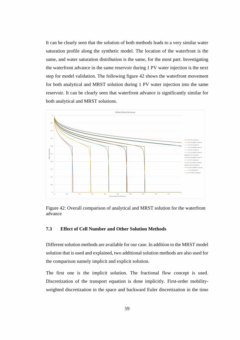
59
It can be clearly seen that the solution of both methods leads to a very similar water
saturation profile along the synthetic model. The location of the waterfront is the
same, and water saturation distribution is the same, for the most part. Investigating
the waterfront advance in the same reservoir during 1 PV water injection is the next
step for model validation. The following figure 42 shows the waterfront movement
for both analytical and MRST solution during 1 PV water injection into the same
reservoir. It can be clearly seen that waterfront advance is significantly similar for
both analytical and MRST solutions.
Figure 42: Overall comparison of analytical and MRST solution for the waterfront
advance
7.3 Effect of Cell Number and Other Solution Methods
Different solution methods are available for our case. In addition to the MRST model
solution that is used and explained, two additional solution methods are also used for
the comparison namely implicit and explicit solution.
The first one is the implicit solution. The fractional flow concept is used.
Discretization of the transport equation is done implicitly. First-order mobility-
weighted discretization in the space and backward Euler discretization in the time
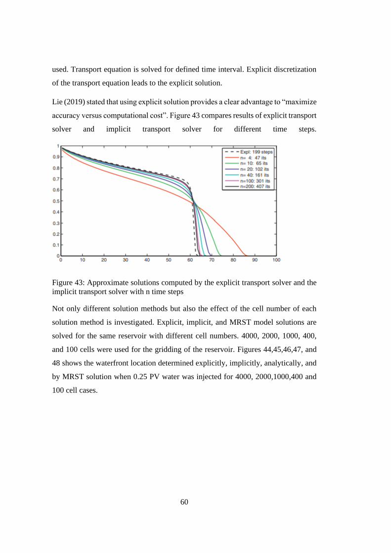
60
used. Transport equation is solved for defined time interval. Explicit discretization
of the transport equation leads to the explicit solution.
Lie (2019) stated that using explicit solution provides a clear advantage to “maximize
accuracy versus computational cost”. Figure 43 compares results of explicit transport
solver and implicit transport solver for different time steps.
Figure 43: Approximate solutions computed by the explicit transport solver and the
implicit transport solver with n time steps
Not only different solution methods but also the effect of the cell number of each
solution method is investigated. Explicit, implicit, and MRST model solutions are
solved for the same reservoir with different cell numbers. 4000, 2000, 1000, 400,
and 100 cells were used for the gridding of the reservoir. Figures 44,45,46,47, and
48 shows the waterfront location determined explicitly, implicitly, analytically, and
by MRST solution when 0.25 PV water was injected for 4000, 2000,1000,400 and
100 cell cases.
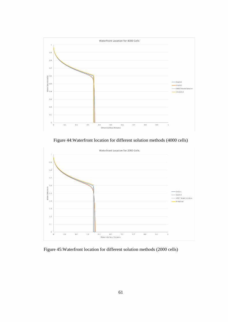
61
Figure 44:Waterfront location for different solution methods (4000 cells)
Figure 45:Waterfront location for different solution methods (2000 cells)
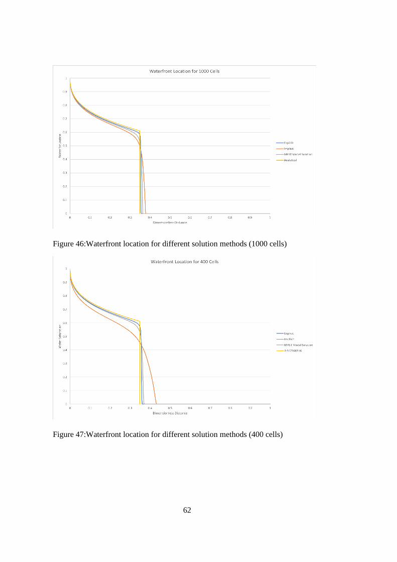
62
Figure 46:Waterfront location for different solution methods (1000 cells)
Figure 47:Waterfront location for different solution methods (400 cells)
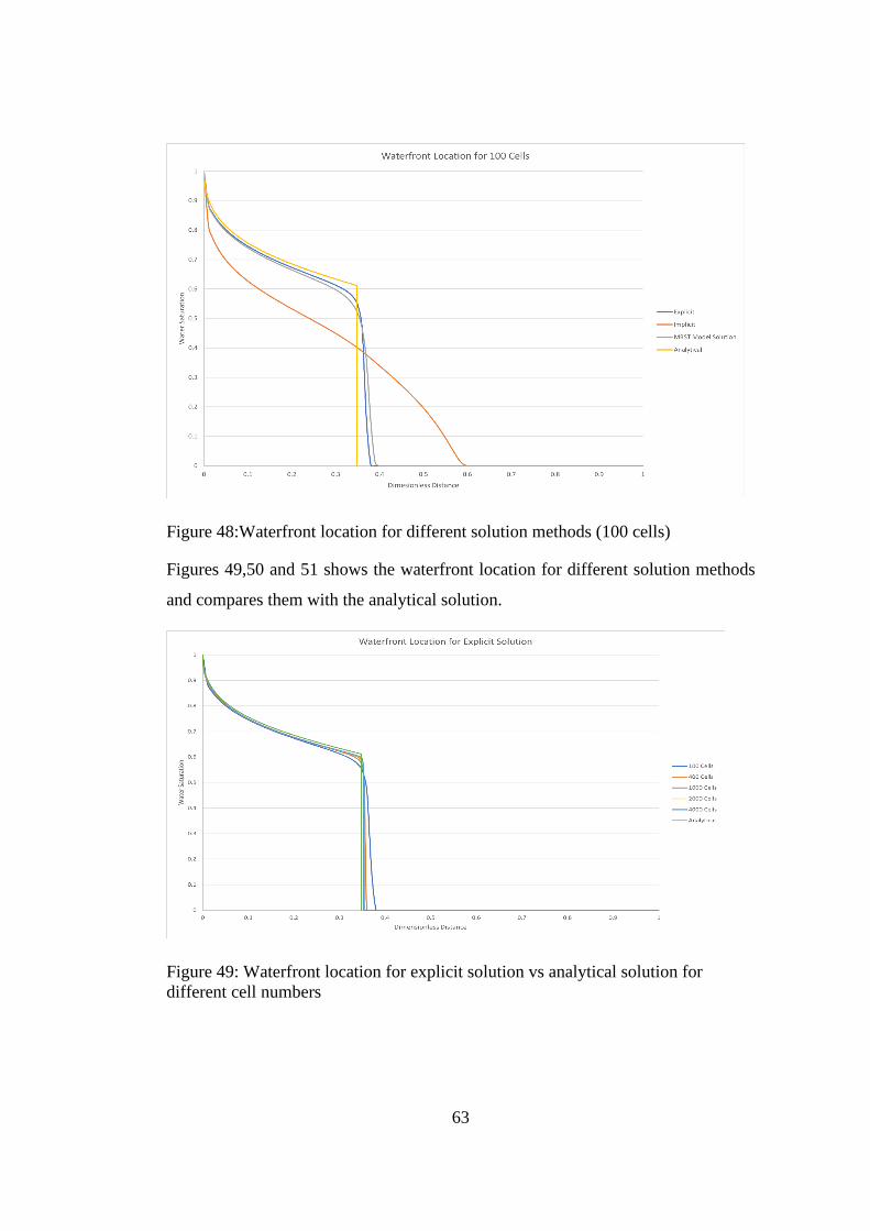
63
Figure 48:Waterfront location for different solution methods (100 cells)
Figures 49,50 and 51 shows the waterfront location for different solution methods
and compares them with the analytical solution.
Figure 49: Waterfront location for explicit solution vs analytical solution for
different cell numbers
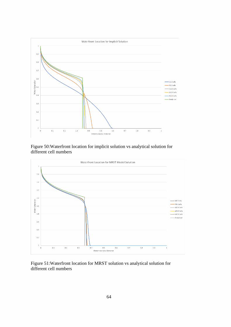
64
Figure 50:Waterfront location for implicit solution vs analytical solution for
different cell numbers
Figure 51:Waterfront location for MRST solution vs analytical solution for
different cell numbers
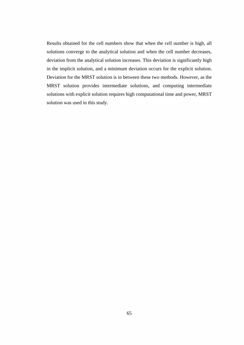
65
Results obtained for the cell numbers show that when the cell number is high, all
solutions converge to the analytical solution and when the cell number decreases,
deviation from the analytical solution increases. This deviation is significantly high
in the implicit solution, and a minimum deviation occurs for the explicit solution.
Deviation for the MRST solution is in between these two methods. However, as the
MRST solution provides intermediate solutions, and computing intermediate
solutions with explicit solution requires high computational time and power, MRST
solution was used in this study.

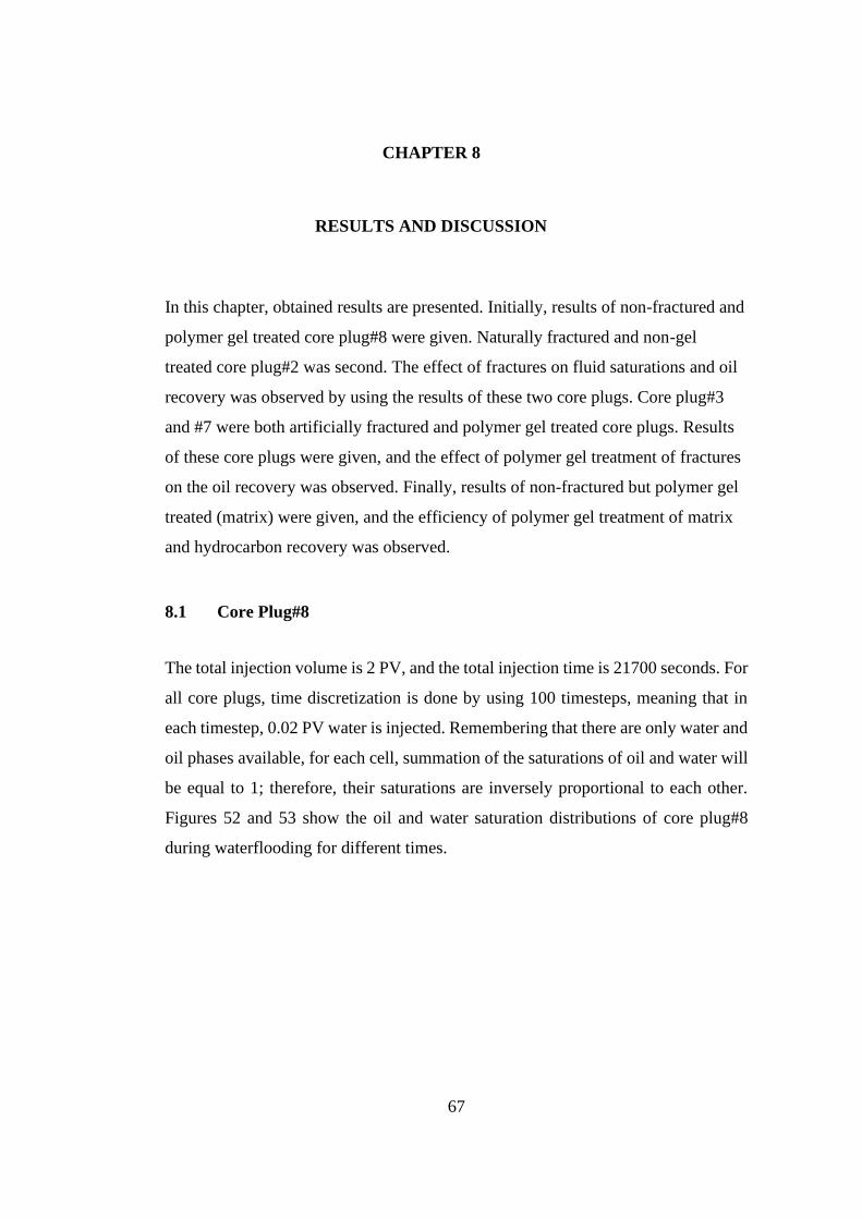
67
CHAPTER 8
8 RESULTS AND DISCUSSION
In this chapter, obtained results are presented. Initially, results of non-fractured and
polymer gel treated core plug#8 were given. Naturally fractured and non-gel
treated core plug#2 was second. The effect of fractures on fluid saturations and oil
recovery was observed by using the results of these two core plugs. Core plug#3
and #7 were both artificially fractured and polymer gel treated core plugs. Results
of these core plugs were given, and the effect of polymer gel treatment of fractures
on the oil recovery was observed. Finally, results of non-fractured but polymer gel
treated (matrix) were given, and the efficiency of polymer gel treatment of matrix
and hydrocarbon recovery was observed.
8.1 Core Plug#8
The total injection volume is 2 PV, and the total injection time is 21700 seconds. For
all core plugs, time discretization is done by using 100 timesteps, meaning that in
each timestep, 0.02 PV water is injected. Remembering that there are only water and
oil phases available, for each cell, summation of the saturations of oil and water will
be equal to 1; therefore, their saturations are inversely proportional to each other.
Figures 52 and 53 show the oil and water saturation distributions of core plug#8
during waterflooding for different times.
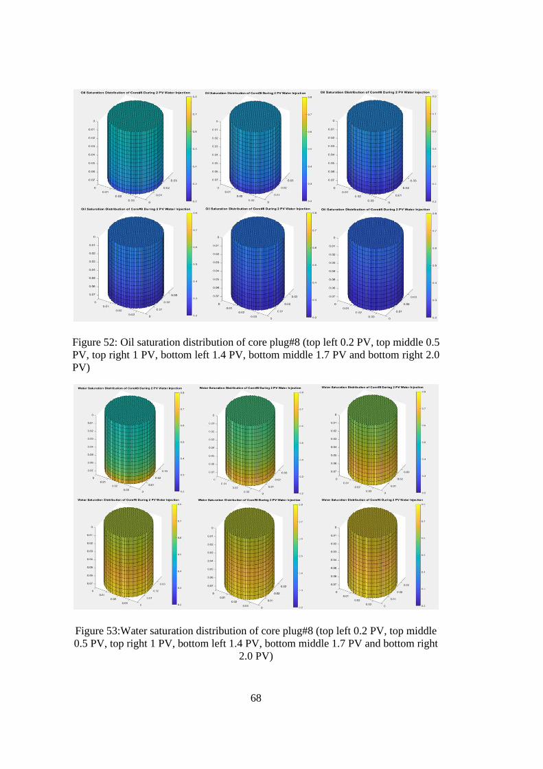
68
Figure 52: Oil saturation distribution of core plug#8 (top left 0.2 PV, top middle 0.5
PV, top right 1 PV, bottom left 1.4 PV, bottom middle 1.7 PV and bottom right 2.0
PV)
Figure 53:Water saturation distribution of core plug#8 (top left 0.2 PV, top middle
0.5 PV, top right 1 PV, bottom left 1.4 PV, bottom middle 1.7 PV and bottom right
2.0 PV)
69
Although MRST can easily obtain the fluid saturation for the core plugs for different
times, corresponding experimental results, are not available. An average saturation
for different layers is available. Therefore, final water saturation plots are compared.
Figure 54 shows the water saturations for each layer obtained experimentally and
with simulations.
Figure 54: Water saturation profile of core plug#8
Considering the fact that core plug is modeled vertically, obtained trend (higher
water saturations at the bottom and lower water saturations in the upper layers) is
reasonable. In addition, gravity leads to higher water saturation in the bottom layers.
Experimentally, water saturation in the bottom layers (layers 2 and 3 is significantly
higher than the remaining layers, and for the top five layers, water saturation is
significantly low. Additionally, the mean water saturation of the core plug
experimentally determined as 0.694 and similarly 0.7026 was the result of the
simulations.
Another vital parameter to check experiment and simulation results is the recovery
of hydrocarbons. As waterflooding is done to increase recovery, it is crucial to have
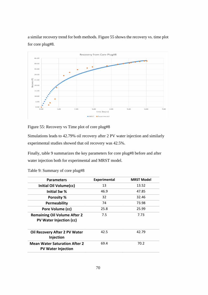
70
a similar recovery trend for both methods. Figure 55 shows the recovery vs. time plot
for core plug#8.
Figure 55: Recovery vs Time plot of core plug#8
Simulations leads to 42.79% oil recovery after 2 PV water injection and similarly
experimental studies showed that oil recovery was 42.5%.
Finally, table 9 summarizes the key parameters for core plug#8 before and after
water injection both for experimental and MRST model.
Table 9: Summary of core plug#8
Parameters Experimental MRST Model
Initial Oil Volume(cc) 13 13.52
Initial Sw % 46.9 47.85
Porosity % 32 32.46
Permeability 74 73.98
Pore Volume (cc) 25.8 25.99
Remaining Oil Volume After 2 PV Water Injection (cc)
7.5 7.73
Oil Recovery After 2 PV Water Injection
42.5 42.79
Mean Water Saturation After 2 PV Water Injection
69.4 70.2
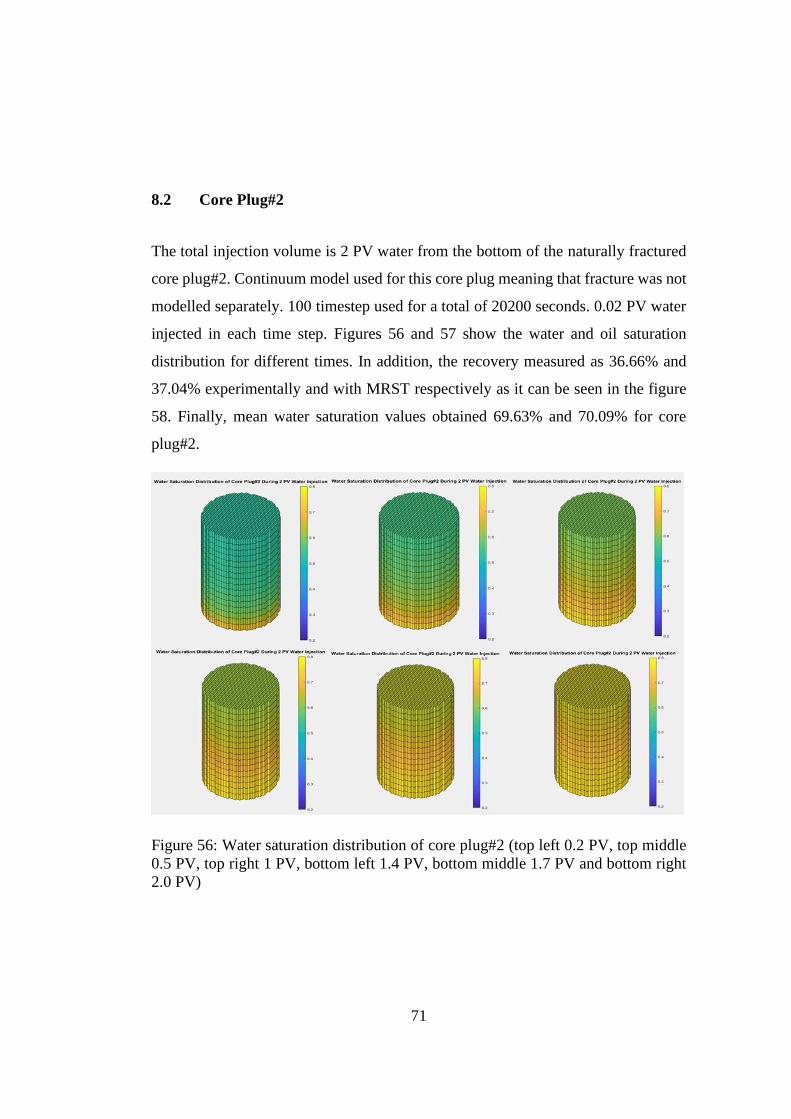
71
8.2 Core Plug#2
The total injection volume is 2 PV water from the bottom of the naturally fractured
core plug#2. Continuum model used for this core plug meaning that fracture was not
modelled separately. 100 timestep used for a total of 20200 seconds. 0.02 PV water
injected in each time step. Figures 56 and 57 show the water and oil saturation
distribution for different times. In addition, the recovery measured as 36.66% and
37.04% experimentally and with MRST respectively as it can be seen in the figure
58. Finally, mean water saturation values obtained 69.63% and 70.09% for core
plug#2.
Figure 56: Water saturation distribution of core plug#2 (top left 0.2 PV, top middle
0.5 PV, top right 1 PV, bottom left 1.4 PV, bottom middle 1.7 PV and bottom right
2.0 PV)
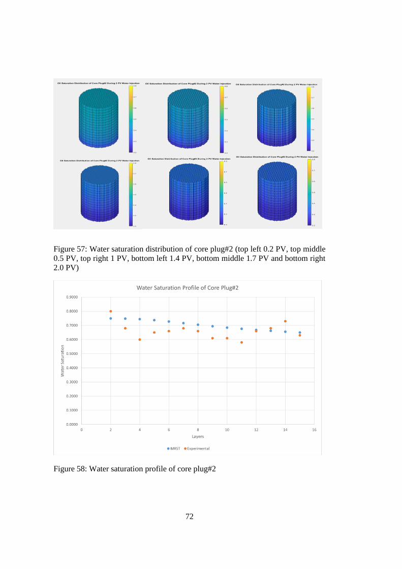
72
Figure 57: Water saturation distribution of core plug#2 (top left 0.2 PV, top middle
0.5 PV, top right 1 PV, bottom left 1.4 PV, bottom middle 1.7 PV and bottom right
2.0 PV)
Figure 58: Water saturation profile of core plug#2
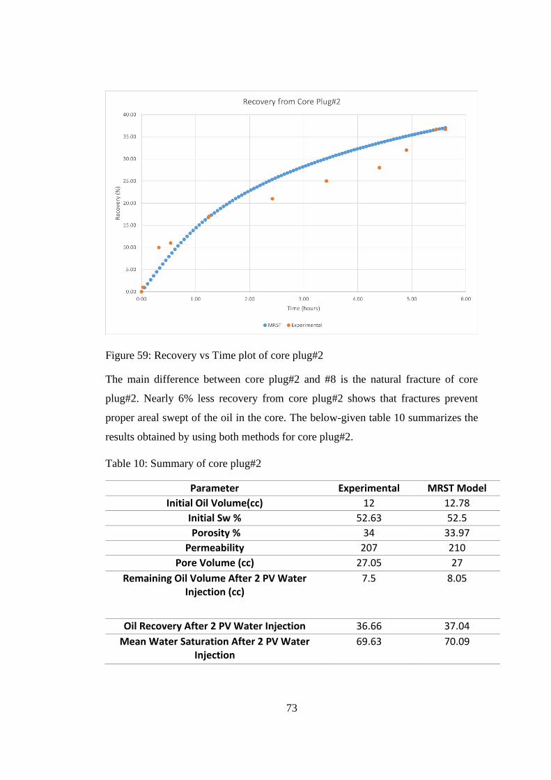
73
Figure 59: Recovery vs Time plot of core plug#2
The main difference between core plug#2 and #8 is the natural fracture of core
plug#2. Nearly 6% less recovery from core plug#2 shows that fractures prevent
proper areal swept of the oil in the core. The below-given table 10 summarizes the
results obtained by using both methods for core plug#2.
Table 10: Summary of core plug#2
Parameter Experimental MRST Model
Initial Oil Volume(cc) 12 12.78
Initial Sw % 52.63 52.5
Porosity % 34 33.97
Permeability 207 210
Pore Volume (cc) 27.05 27
Remaining Oil Volume After 2 PV Water Injection (cc)
7.5 8.05
Oil Recovery After 2 PV Water Injection 36.66 37.04
Mean Water Saturation After 2 PV Water Injection
69.63 70.09
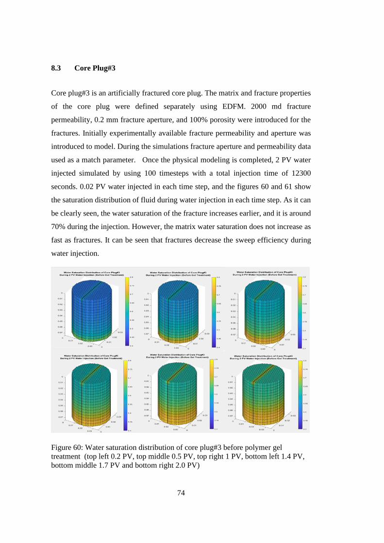
74
8.3 Core Plug#3
Core plug#3 is an artificially fractured core plug. The matrix and fracture properties
of the core plug were defined separately using EDFM. 2000 md fracture
permeability, 0.2 mm fracture aperture, and 100% porosity were introduced for the
fractures. Initially experimentally available fracture permeability and aperture was
introduced to model. During the simulations fracture aperture and permeability data
used as a match parameter. Once the physical modeling is completed, 2 PV water
injected simulated by using 100 timesteps with a total injection time of 12300
seconds. 0.02 PV water injected in each time step, and the figures 60 and 61 show
the saturation distribution of fluid during water injection in each time step. As it can
be clearly seen, the water saturation of the fracture increases earlier, and it is around
70% during the injection. However, the matrix water saturation does not increase as
fast as fractures. It can be seen that fractures decrease the sweep efficiency during
water injection.
Figure 60: Water saturation distribution of core plug#3 before polymer gel
treatment (top left 0.2 PV, top middle 0.5 PV, top right 1 PV, bottom left 1.4 PV,
bottom middle 1.7 PV and bottom right 2.0 PV)
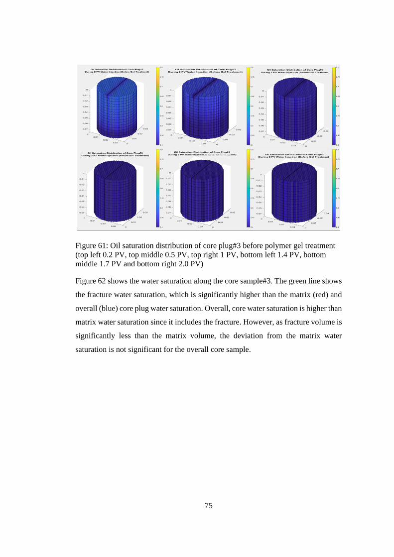
75
Figure 61: Oil saturation distribution of core plug#3 before polymer gel treatment
(top left 0.2 PV, top middle 0.5 PV, top right 1 PV, bottom left 1.4 PV, bottom
middle 1.7 PV and bottom right 2.0 PV)
Figure 62 shows the water saturation along the core sample#3. The green line shows
the fracture water saturation, which is significantly higher than the matrix (red) and
overall (blue) core plug water saturation. Overall, core water saturation is higher than
matrix water saturation since it includes the fracture. However, as fracture volume is
significantly less than the matrix volume, the deviation from the matrix water
saturation is not significant for the overall core sample.
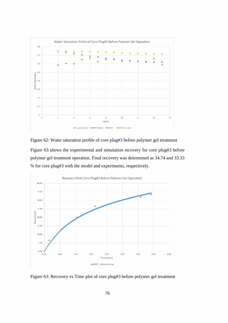
76
Figure 62: Water saturation profile of core plug#3 before polymer gel treatment
Figure 63 shows the experimental and simulation recovery for core plug#3 before
polymer gel treatment operation. Final recovery was determined as 34.74 and 33.33
% for core plug#3 with the model and experiments, respectively.
Figure 63: Recovery vs Time plot of core plug#3 before polymer gel treatment
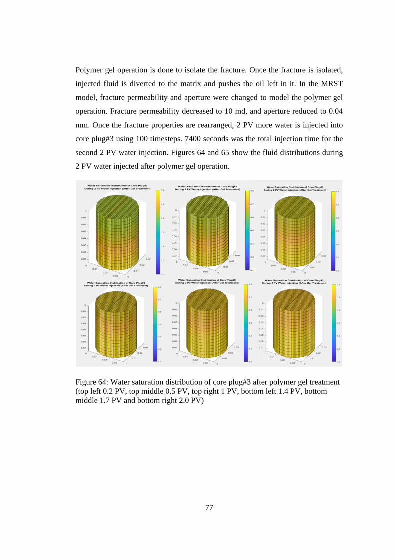
77
Polymer gel operation is done to isolate the fracture. Once the fracture is isolated,
injected fluid is diverted to the matrix and pushes the oil left in it. In the MRST
model, fracture permeability and aperture were changed to model the polymer gel
operation. Fracture permeability decreased to 10 md, and aperture reduced to 0.04
mm. Once the fracture properties are rearranged, 2 PV more water is injected into
core plug#3 using 100 timesteps. 7400 seconds was the total injection time for the
second 2 PV water injection. Figures 64 and 65 show the fluid distributions during
2 PV water injected after polymer gel operation.
Figure 64: Water saturation distribution of core plug#3 after polymer gel treatment
(top left 0.2 PV, top middle 0.5 PV, top right 1 PV, bottom left 1.4 PV, bottom
middle 1.7 PV and bottom right 2.0 PV)
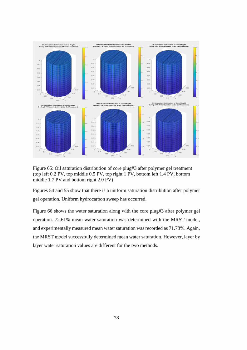
78
Figure 65: Oil saturation distribution of core plug#3 after polymer gel treatment
(top left 0.2 PV, top middle 0.5 PV, top right 1 PV, bottom left 1.4 PV, bottom
middle 1.7 PV and bottom right 2.0 PV)
Figures 54 and 55 show that there is a uniform saturation distribution after polymer
gel operation. Uniform hydrocarbon sweep has occurred.
Figure 66 shows the water saturation along with the core plug#3 after polymer gel
operation. 72.61% mean water saturation was determined with the MRST model,
and experimentally measured mean water saturation was recorded as 71.78%. Again,
the MRST model successfully determined mean water saturation. However, layer by
layer water saturation values are different for the two methods.
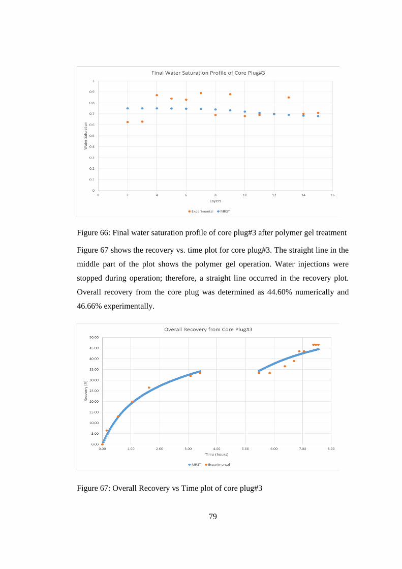
79
Figure 66: Final water saturation profile of core plug#3 after polymer gel treatment
Figure 67 shows the recovery vs. time plot for core plug#3. The straight line in the
middle part of the plot shows the polymer gel operation. Water injections were
stopped during operation; therefore, a straight line occurred in the recovery plot.
Overall recovery from the core plug was determined as 44.60% numerically and
46.66% experimentally.
Figure 67: Overall Recovery vs Time plot of core plug#3
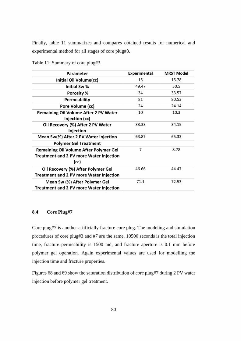
80
Finally, table 11 summarizes and compares obtained results for numerical and
experimental method for all stages of core plug#3.
Table 11: Summary of core plug#3
Parameter Experimental MRST Model
Initial Oil Volume(cc) 15 15.78
Initial Sw % 49.47 50.5
Porosity % 34 33.57
Permeability 81 80.53
Pore Volume (cc) 24 24.14
Remaining Oil Volume After 2 PV Water Injection (cc)
10 10.3
Oil Recovery (%) After 2 PV Water Injection
33.33 34.15
Mean Sw(%) After 2 PV Water Injection 63.87 65.33
Polymer Gel Treatment
Remaining Oil Volume After Polymer Gel Treatment and 2 PV more Water Injection
(cc)
7 8.78
Oil Recovery (%) After Polymer Gel Treatment and 2 PV more Water Injection
46.66 44.47
Mean Sw (%) After Polymer Gel Treatment and 2 PV more Water Injection
71.1 72.53
8.4 Core Plug#7
Core plug#7 is another artificially fracture core plug. The modeling and simulation
procedures of core plug#3 and #7 are the same. 10500 seconds is the total injection
time, fracture permeability is 1500 md, and fracture aperture is 0.1 mm before
polymer gel operation. Again experimental values are used for modelling the
injection time and fracture properties.
Figures 68 and 69 show the saturation distribution of core plug#7 during 2 PV water
injection before polymer gel treatment.
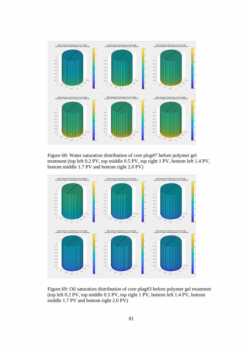
81
Figure 68: Water saturation distribution of core plug#7 before polymer gel
treatment (top left 0.2 PV, top middle 0.5 PV, top right 1 PV, bottom left 1.4 PV,
bottom middle 1.7 PV and bottom right 2.0 PV)
Figure 69: Oil saturation distribution of core plug#3 before polymer gel treatment
(top left 0.2 PV, top middle 0.5 PV, top right 1 PV, bottom left 1.4 PV, bottom
middle 1.7 PV and bottom right 2.0 PV)
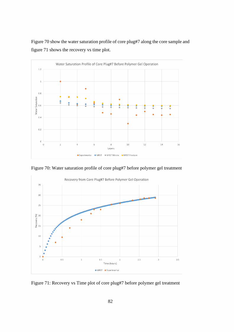
82
Figure 70 show the water saturation profile of core plug#7 along the core sample and
figure 71 shows the recovery vs time plot.
Figure 70: Water saturation profile of core plug#7 before polymer gel treatment
Figure 71: Recovery vs Time plot of core plug#7 before polymer gel treatment
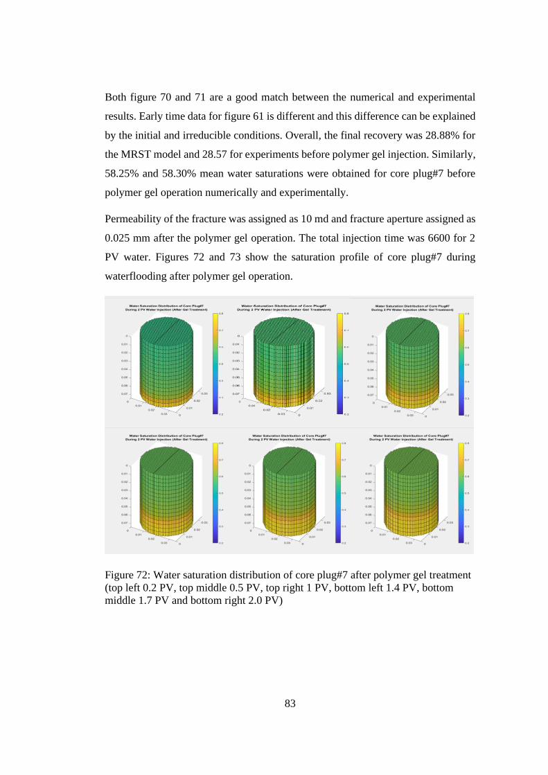
83
Both figure 70 and 71 are a good match between the numerical and experimental
results. Early time data for figure 61 is different and this difference can be explained
by the initial and irreducible conditions. Overall, the final recovery was 28.88% for
the MRST model and 28.57 for experiments before polymer gel injection. Similarly,
58.25% and 58.30% mean water saturations were obtained for core plug#7 before
polymer gel operation numerically and experimentally.
Permeability of the fracture was assigned as 10 md and fracture aperture assigned as
0.025 mm after the polymer gel operation. The total injection time was 6600 for 2
PV water. Figures 72 and 73 show the saturation profile of core plug#7 during
waterflooding after polymer gel operation.
Figure 72: Water saturation distribution of core plug#7 after polymer gel treatment
(top left 0.2 PV, top middle 0.5 PV, top right 1 PV, bottom left 1.4 PV, bottom
middle 1.7 PV and bottom right 2.0 PV)
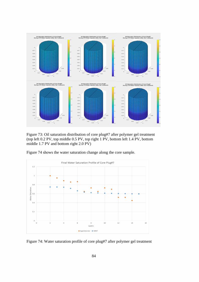
84
Figure 73: Oil saturation distribution of core plug#7 after polymer gel treatment
(top left 0.2 PV, top middle 0.5 PV, top right 1 PV, bottom left 1.4 PV, bottom
middle 1.7 PV and bottom right 2.0 PV)
Figure 74 shows the water saturation change along the core sample.
Figure 74: Water saturation profile of core plug#7 after polymer gel treatment
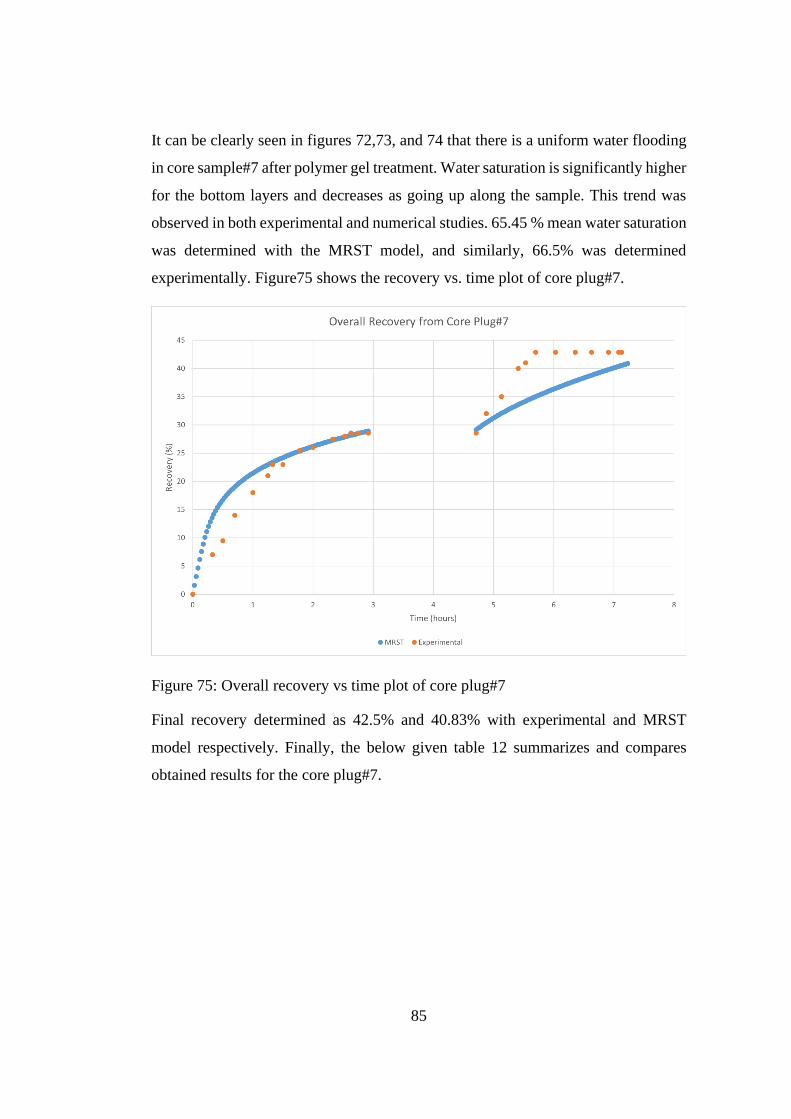
85
It can be clearly seen in figures 72,73, and 74 that there is a uniform water flooding
in core sample#7 after polymer gel treatment. Water saturation is significantly higher
for the bottom layers and decreases as going up along the sample. This trend was
observed in both experimental and numerical studies. 65.45 % mean water saturation
was determined with the MRST model, and similarly, 66.5% was determined
experimentally. Figure75 shows the recovery vs. time plot of core plug#7.
Figure 75: Overall recovery vs time plot of core plug#7
Final recovery determined as 42.5% and 40.83% with experimental and MRST
model respectively. Finally, the below given table 12 summarizes and compares
obtained results for the core plug#7.
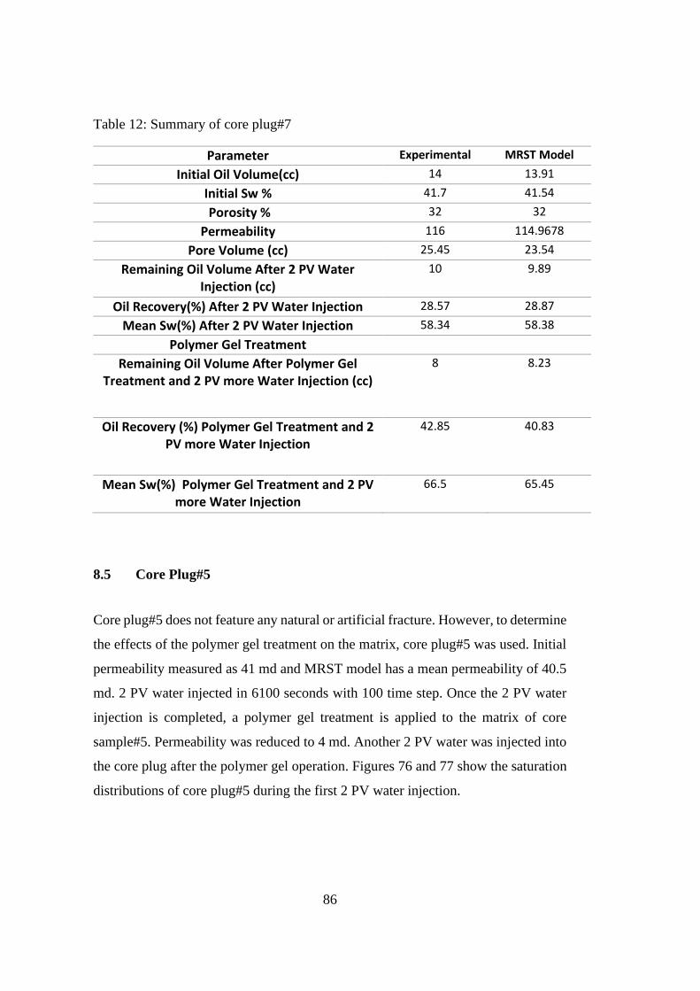
86
Table 12: Summary of core plug#7
Parameter Experimental MRST Model
Initial Oil Volume(cc) 14 13.91
Initial Sw % 41.7 41.54
Porosity % 32 32
Permeability 116 114.9678
Pore Volume (cc) 25.45 23.54
Remaining Oil Volume After 2 PV Water Injection (cc)
10 9.89
Oil Recovery(%) After 2 PV Water Injection 28.57 28.87
Mean Sw(%) After 2 PV Water Injection 58.34 58.38
Polymer Gel Treatment
Remaining Oil Volume After Polymer Gel Treatment and 2 PV more Water Injection (cc)
8 8.23
Oil Recovery (%) Polymer Gel Treatment and 2 PV more Water Injection
42.85 40.83
Mean Sw(%) Polymer Gel Treatment and 2 PV more Water Injection
66.5 65.45
8.5 Core Plug#5
Core plug#5 does not feature any natural or artificial fracture. However, to determine
the effects of the polymer gel treatment on the matrix, core plug#5 was used. Initial
permeability measured as 41 md and MRST model has a mean permeability of 40.5
md. 2 PV water injected in 6100 seconds with 100 time step. Once the 2 PV water
injection is completed, a polymer gel treatment is applied to the matrix of core
sample#5. Permeability was reduced to 4 md. Another 2 PV water was injected into
the core plug after the polymer gel operation. Figures 76 and 77 show the saturation
distributions of core plug#5 during the first 2 PV water injection.
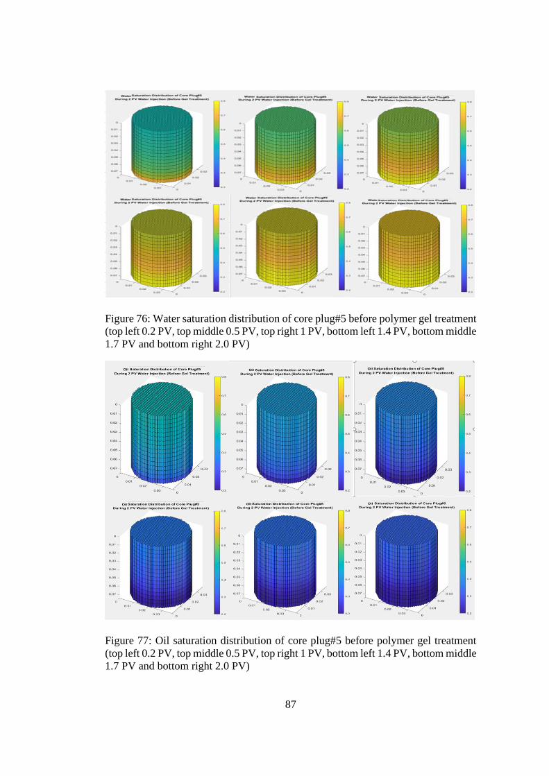
87
Figure 76: Water saturation distribution of core plug#5 before polymer gel treatment
(top left 0.2 PV, top middle 0.5 PV, top right 1 PV, bottom left 1.4 PV, bottom middle
1.7 PV and bottom right 2.0 PV)
Figure 77: Oil saturation distribution of core plug#5 before polymer gel treatment
(top left 0.2 PV, top middle 0.5 PV, top right 1 PV, bottom left 1.4 PV, bottom middle
1.7 PV and bottom right 2.0 PV)
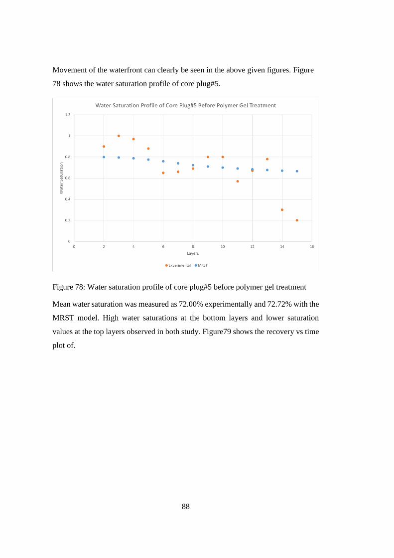
88
Movement of the waterfront can clearly be seen in the above given figures. Figure
78 shows the water saturation profile of core plug#5.
Figure 78: Water saturation profile of core plug#5 before polymer gel treatment
Mean water saturation was measured as 72.00% experimentally and 72.72% with the
MRST model. High water saturations at the bottom layers and lower saturation
values at the top layers observed in both study. Figure79 shows the recovery vs time
plot of.
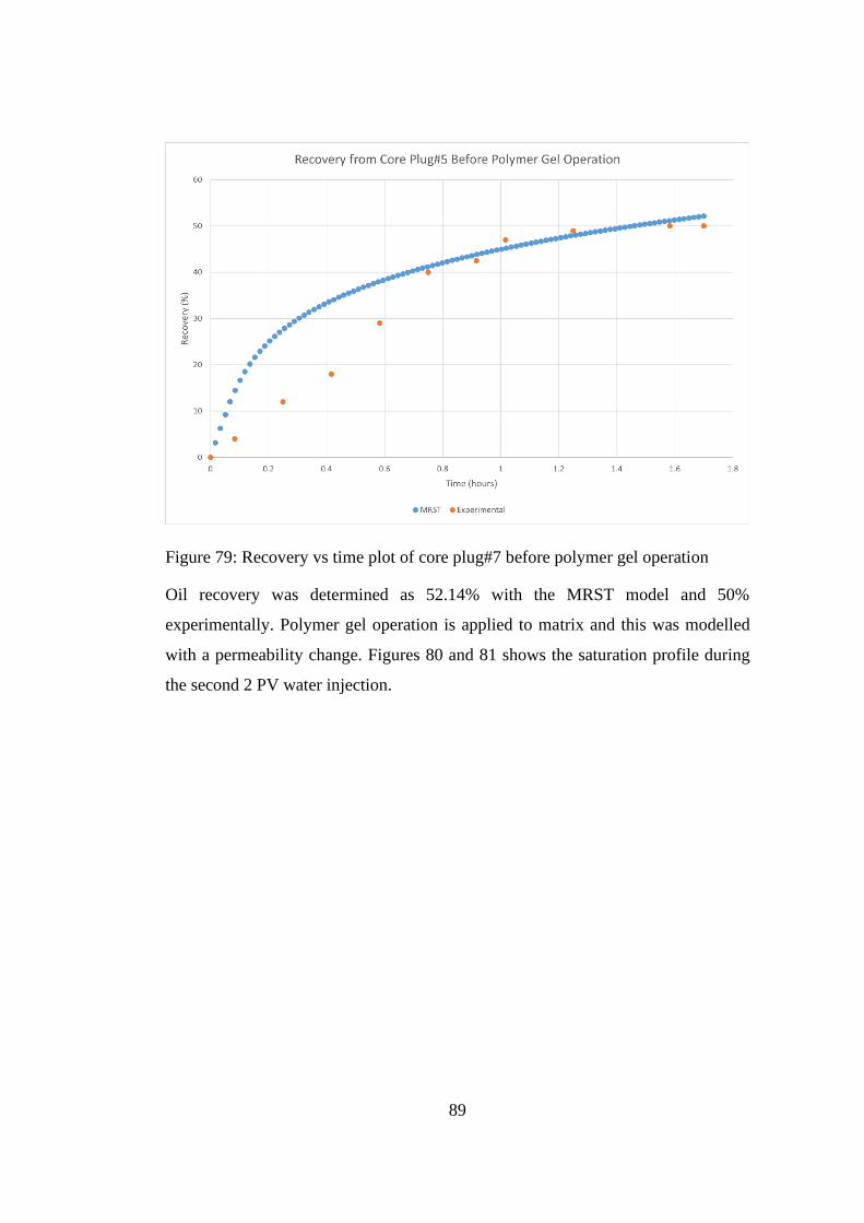
89
Figure 79: Recovery vs time plot of core plug#7 before polymer gel operation
Oil recovery was determined as 52.14% with the MRST model and 50%
experimentally. Polymer gel operation is applied to matrix and this was modelled
with a permeability change. Figures 80 and 81 shows the saturation profile during
the second 2 PV water injection.
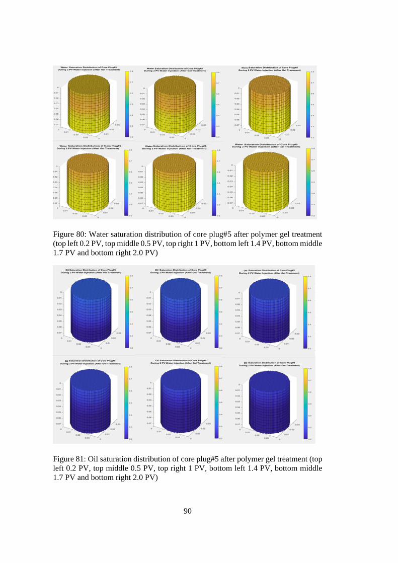
90
Figure 80: Water saturation distribution of core plug#5 after polymer gel treatment
(top left 0.2 PV, top middle 0.5 PV, top right 1 PV, bottom left 1.4 PV, bottom middle
1.7 PV and bottom right 2.0 PV)
Figure 81: Oil saturation distribution of core plug#5 after polymer gel treatment (top
left 0.2 PV, top middle 0.5 PV, top right 1 PV, bottom left 1.4 PV, bottom middle
1.7 PV and bottom right 2.0 PV)
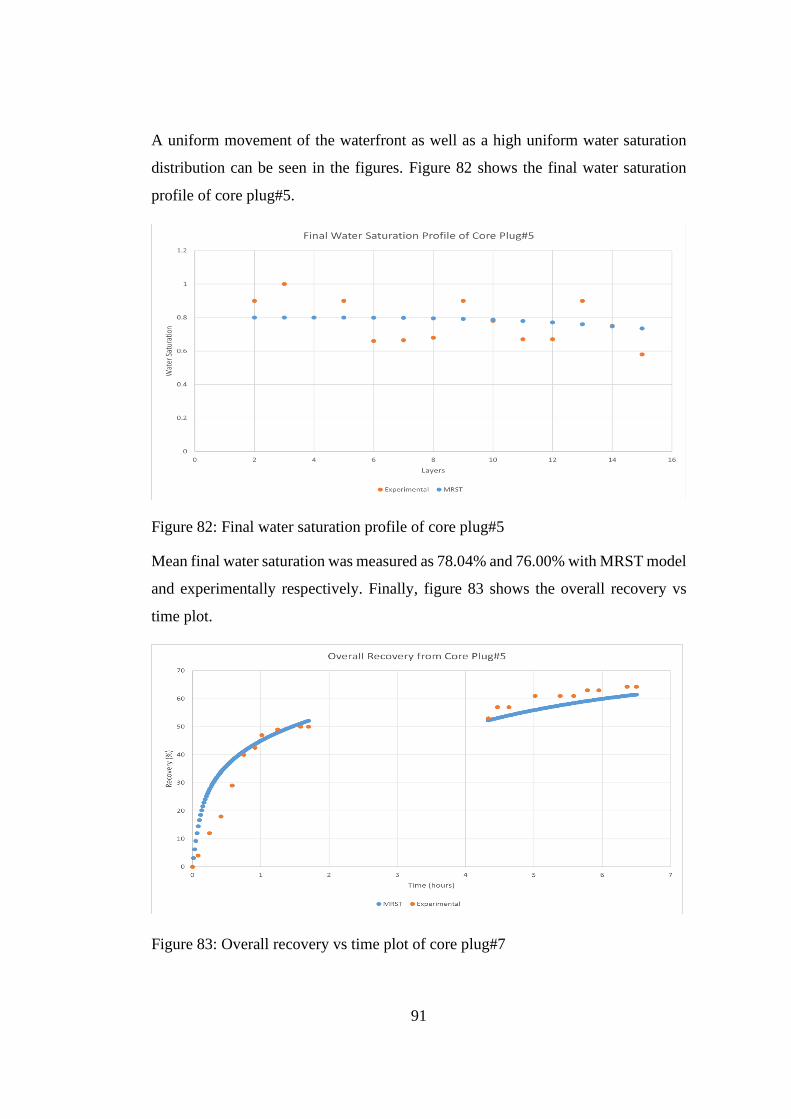
91
A uniform movement of the waterfront as well as a high uniform water saturation
distribution can be seen in the figures. Figure 82 shows the final water saturation
profile of core plug#5.
Figure 82: Final water saturation profile of core plug#5
Mean final water saturation was measured as 78.04% and 76.00% with MRST model
and experimentally respectively. Finally, figure 83 shows the overall recovery vs
time plot.
Figure 83: Overall recovery vs time plot of core plug#7
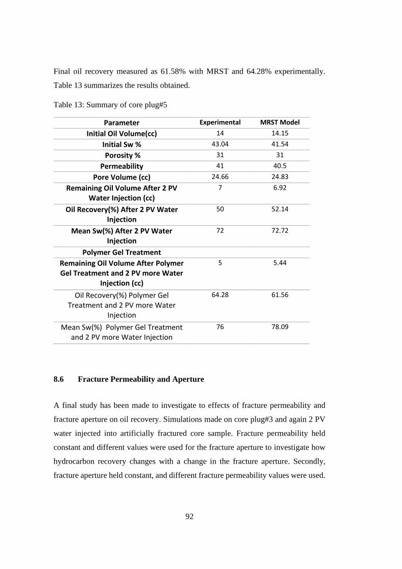
92
Final oil recovery measured as 61.58% with MRST and 64.28% experimentally.
Table 13 summarizes the results obtained.
Table 13: Summary of core plug#5
Parameter Experimental MRST Model
Initial Oil Volume(cc) 14 14.15
Initial Sw % 43.04 41.54
Porosity % 31 31
Permeability 41 40.5
Pore Volume (cc) 24.66 24.83
Remaining Oil Volume After 2 PV Water Injection (cc)
7 6.92
Oil Recovery(%) After 2 PV Water Injection
50 52.14
Mean Sw(%) After 2 PV Water Injection
72 72.72
Polymer Gel Treatment
Remaining Oil Volume After Polymer Gel Treatment and 2 PV more Water
Injection (cc)
5 5.44
Oil Recovery(%) Polymer Gel Treatment and 2 PV more Water
Injection
64.28 61.56
Mean Sw(%) Polymer Gel Treatment and 2 PV more Water Injection
76 78.09
8.6 Fracture Permeability and Aperture
A final study has been made to investigate to effects of fracture permeability and
fracture aperture on oil recovery. Simulations made on core plug#3 and again 2 PV
water injected into artificially fractured core sample. Fracture permeability held
constant and different values were used for the fracture aperture to investigate how
hydrocarbon recovery changes with a change in the fracture aperture. Secondly,
fracture aperture held constant, and different fracture permeability values were used.
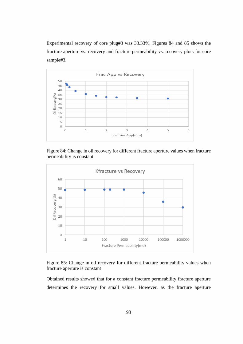
93
Experimental recovery of core plug#3 was 33.33%. Figures 84 and 85 shows the
fracture aperture vs. recovery and fracture permeability vs. recovery plots for core
sample#3.
Figure 84: Change in oil recovery for different fracture aperture values when fracture
permeability is constant
Figure 85: Change in oil recovery for different fracture permeability values when
fracture aperture is constant
Obtained results showed that for a constant fracture permeability fracture aperture
determines the recovery for small values. However, as the fracture aperture

94
increases, recovery remains constant. Similarly, fracture permeability increases leads
to a decrease in the oil recovery for large permeability values. For lower
permeability, recovery does not change significantly when the fracture aperture is
constant.
95
CHAPTER 9
9 CONCLUSION
Lorem This research provides a modeling solution to experimental study. MRST was
used to obtain similar results of the experimental core flooding study. In particular,
different core plugs were modeled by using MRST, and fractures and gel treatment
were introduced to create models to represent the experiment. The non-fractured core
plug model, fractured core plug model, and fractured and gel-treated core plug model
were the three main models created by MRST. Results of the experimental study and
simulations were compared.
Initially, validation of the MRST code is done using the Buckley-Leveret analytical
solution. Comparison of the analytical solution, implicit solution, explicit solution,
and MRST model solution for different cell numbers validated the MRST model
used.
Results of the MRST model showed that having natural fractures decreases oil
recovery. Polymer gel treatment increases the hydrocarbon recovery by reducing the
fracture aperture and permeability. Experimental results and simulation results were
significantly close for the recovery. Mean water saturation was also in an acceptable
error margin. However, layer by layer water saturations were significantly different
for experimental and MRST model results. A single rock and fluid model was
imposed in the MRST model, meaning that minimum and maximum fluid saturations
are the same in each layer. However, experimental results show that different min
and max values are possible for different layers. Therefore, some deviations occurred
from the experiments in the MRST model. In addition, water saturation values had a
common trend along the z-axis for the results of experiments and simulations.
Finally, the effects of the fracture aperture and fracture permeability on the recovery
were investigated. Fracture aperture directly impacts the recovery for the low

96
aperture values when the permeability is constant. Similarly, permeability directly
affects recovery for high values when the aperture is constant.
97
REFERENCES
Abdallah Edmonton, W., Jill Buckley, C. S., Carnegie Kuala Lumpur, A., John
Edwards Bernd Herold Muscat, M., Graue, A., Habashy Nikita Seleznev
Claude Signer, T., Hussain Petroleum Development Oman Muscat, H.,
Bernard Montaron Dubai, O., Murtaza Ziauddin Abu Dhabi, U., Boyd, A.,
Leu, G., Prioul, R., Kennedy, R., Ligneul, P., Arabia, S., McCullagh, J., Land,
S., & Picard, G. (n.d.). Fundamentals of Wettability.
AlSofi, A. M., & Yousef, A. A. (2013). Insight into smart-water recovery
mechanism through detailed history matching of coreflood experiments.
Society of Petroleum Engineers - SPE Reservoir Characterisation and
Simulation Conference and Exhibition, RCSC 2013: New Approaches in
Characterisation AndModelling of Complex Reservoirs, 2, 965–976.
https://doi.org/10.2118/166035-ms
Brattekås, B., & Seright, R. S. (2018). Implications for improved polymer gel
conformance control during low-salinity chase-floods in fractured carbonates.
Journal of Petroleum Science and Engineering, 163, 661–670.
https://doi.org/10.1016/j.petrol.2017.10.033
Brown, G. O. (2003). The History of the Darcy-Weisbach Equation for Pipe Flow
Resistance. Environmental and Water Resources History, 34–43.
Bryant, S., & Blunt, M. (1992). Prediction of relative permeability in simple porous
media. Physical Review A, 46(4), 2004–2011.
https://doi.org/10.1103/PhysRevA.46.2004
Buckley, S. E., & Leverett, M. C. (1942). Mechanism of Fluid Displacement in
Sands. Transactions of the AIME, 146(01), 107–116.
https://doi.org/10.2118/942107-g
Canbolat, S., & Parlaktuna, M. (2019). Polymer gel conformance on oil recovery in
98
fractured medium: Visualization and verification. Journal of Petroleum
Science and Engineering, 182, 106289.
https://doi.org/10.1016/j.petrol.2019.106289
Chen, Y., Xie, Q., Sari, A., Brady, P. V., & Saeedi, A. (2018). Oil/water/rock
wettability: Influencing factors and implications for low salinity water
flooding in carbonate reservoirs. Fuel, 215, 171–177.
https://doi.org/10.1016/j.fuel.2017.10.031
COREY, & T., A. (1954). The interrelation between gas and oil relative
permeabilities. Producers Monthly, 38–41.
http://ci.nii.ac.jp/naid/20001335630/en/
Dachanuwattana, S., Jin, J., Zuloaga-Molero, P., Li, X., Xu, Y., Sepehrnoori, K.,
Yu, W., & Miao, J. (2018). Application of proxy-based MCMC and EDFM to
history match a Vaca Muerta shale oil well. Fuel, 220(February), 490–502.
https://doi.org/10.1016/j.fuel.2018.02.018
Douglas, J., & Arbogast, T. (1989). Dual-Porosity models for flow in naturally
fractured reservoirs. Dynamics of Fluids in Hierarchical Porous Media, 1–39.
Garipov, T. T., Karimi-Fard, M., & Tchelepi, H. A. (2016). Discrete fracture model
for coupled flow and geomechanics. Computational Geosciences, 20(1), 149–
160. https://doi.org/10.1007/s10596-015-9554-z
Herbas, J. G., Moreno, R., Marin, A., Romero, M. F., & Coombe, D. A. (2004).
Reservoir simulation of non selective placement of a polymer gel treatment to
improve water injection profiles and sweep efficiency in the lagomar field
western venezuela. SPE International Petroleum Conference in Mexico -
Proceedings, 551–560. https://doi.org/10.2118/92025-ms
Iglauer, S. (2017). CO2-Water-Rock Wettability: Variability, Influencing Factors,
and Implications for CO2 Geostorage. Accounts of Chemical Research, 50(5),
1134–1142. https://doi.org/10.1021/acs.accounts.6b00602
99
Jiang, J., & Younis, R. M. (2015). A multimechanistic multicontinuum model for
simulating shale gas reservoir with complex fractured system. Fuel, 161, 333–
344. https://doi.org/10.1016/j.fuel.2015.08.069
Johnson, E. F., Bossler, D. P., & Bossler, V. O. N. (1959). Calculation of Relative
Permeability from Displacement Experiments. Transactions of the AIME,
216(01), 370–372. https://doi.org/10.2118/1023-g
Lei, Q., Latham, J. P., & Tsang, C. F. (2017). The use of discrete fracture networks
for modelling coupled geomechanical and hydrological behaviour of fractured
rocks. In Computers and Geotechnics (Vol. 85, pp. 151–176). Elsevier Ltd.
https://doi.org/10.1016/j.compgeo.2016.12.024
Lei, Q., Latham, J. P., Tsang, C. F., Xiang, J., & Lang, P. (2015). A new approach
to upscaling fracture network models while preserving geostatistical and
geomechanical characteristics. Journal of Geophysical Research: Solid Earth,
120(7), 4784–4807. https://doi.org/10.1002/2014JB011736
Lie, K.-A. (2019). An Introduction to Reservoir Simulation Using MATLAB/GNU
Octave.
Liu, J., Wang, J. G., Gao, F., Leung, C. F., & Ma, Z. (2019). A fully coupled
fracture equivalent continuum-dual porosity model for hydro-mechanical
process in fractured shale gas reservoirs. Computers and Geotechnics, 106,
143–160. https://doi.org/10.1016/j.compgeo.2018.10.017
Liu, R., Li, B., & Jiang, Y. (2016). A fractal model based on a new governing
equation of fluid flow in fractures for characterizing hydraulic properties of
rock fracture networks. Computers and Geotechnics, 75, 57–68.
https://doi.org/10.1016/j.compgeo.2016.01.025
Malik, B. (2017). Gas-Water Contacts, Free Water Levels analysis in support of
petroleum exploration in offshore Netherlands.
Morrow, N. R. (1962). WETTED POROUS MEDIA.
100
Nazridoust, K., Ahmadi, G., & Smith, D. H. (2006). A new friction factor
correlation for laminar, single-phase flows through rock fractures. Journal of
Hydrology, 329(1–2), 315–328. https://doi.org/10.1016/j.jhydrol.2006.02.032
Nojabaei, B., Johns, R. T., & Chu, L. (2013). Effect of capillary pressure on phase
behavior in tight rocks and shales. SPE Reservoir Evaluation and
Engineering, 16(3), 281–289. https://doi.org/10.2118/159258-PA
Ouenes, A., & Hartley, L. J. (2000). Integrated fracture reservoir modeling using
both discrete and continuum approaches. Proceedings - SPE Annual Technical
Conference and Exhibition, PI(October), 91–100.
https://doi.org/10.2523/62939-ms
Ranjith, P. G., Choi, S. K., & Fourar, M. (2006). Characterization of two-phase
flow in a single rock joint. International Journal of Rock Mechanics and
Mining Sciences, 43(2), 216–223.
https://doi.org/10.1016/j.ijrmms.2005.06.001
Shakiba, M., Cavalcante Filho, J. S. de A., & Sepehrnoori, K. (2018). Using
Embedded Discrete Fracture Model (EDFM) in numerical simulation of
complex hydraulic fracture networks calibrated by microseismic monitoring
data. Journal of Natural Gas Science and Engineering, 55(April), 495–507.
https://doi.org/10.1016/j.jngse.2018.04.019
Shiriyev, J. (2013). Discrete Fracture Network Modeling (Issue June).
Sydansk, R. . (1988). A New Conformance-Improvement-Treatment Chromium(III)
Gel Technology.
Ţene, M., Bosma, S. B. M., Al Kobaisi, M. S., & Hajibeygi, H. (2017). Projection-
based Embedded Discrete Fracture Model (pEDFM). Advances in Water
Resources, 105, 205–216. https://doi.org/10.1016/j.advwatres.2017.05.009
Warren, J. E., & Root, P. J. (1963). The Behavior of Naturally Fractured
Reservoirs. Society of Petroleum Engineers Journal, 3(03), 245–255.

101
https://doi.org/10.2118/426-pa
Zhang, S., Wei, F., Liu, P., Shao, L., & Li, W. (2020). Plugging mechanisms of
polymer gel used for hydraulic fracture water shutoff. E-Polymers, 20(1),
411–422. https://doi.org/10.1515/epoly-2020-0045
Zimmerman, R. W., & Bodvarsson, G. S. (1996). Hydraulic conductivity of rock
fractures. Transport in Porous Media, 23(1), 1–30.
https://doi.org/10.1007/BF00145263

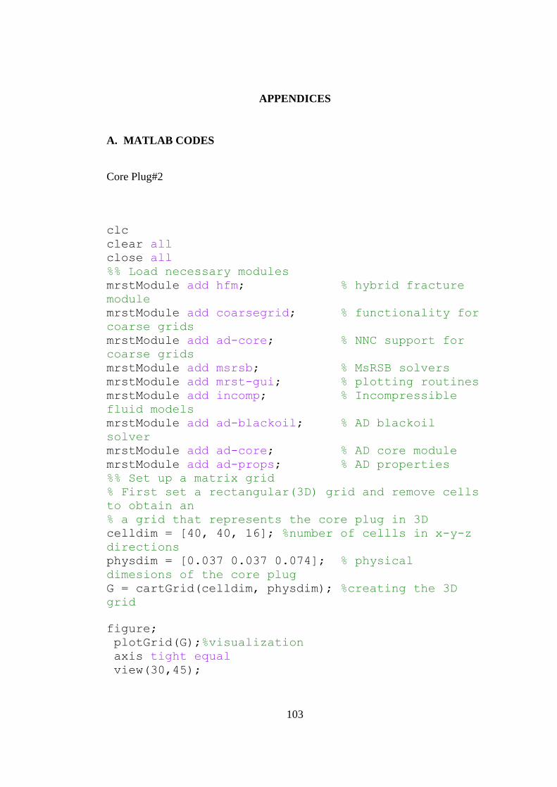
103
APPENDICES
A. MATLAB CODES
Core Plug#2
clc
clear all
close all
%% Load necessary modules
mrstModule add hfm; % hybrid fracture
module
mrstModule add coarsegrid; % functionality for
coarse grids
mrstModule add ad-core; % NNC support for
coarse grids
mrstModule add msrsb; % MsRSB solvers
mrstModule add mrst-gui; % plotting routines
mrstModule add incomp; % Incompressible
fluid models
mrstModule add ad-blackoil; % AD blackoil
solver
mrstModule add ad-core; % AD core module
mrstModule add ad-props; % AD properties
%% Set up a matrix grid
% First set a rectangular(3D) grid and remove cells
to obtain an
% a grid that represents the core plug in 3D
celldim = [40, 40, 16]; %number of cellls in x-y-z
directions
physdim = [0.037 0.037 0.074]; % physical
dimesions of the core plug
G = cartGrid(celldim, physdim); %creating the 3D
grid
figure;
plotGrid(G);%visualization
axis tight equal
view(30,45);
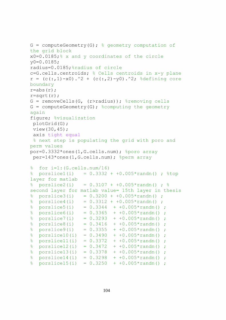
104
G = computeGeometry(G); % geometry computation of
the grid block
x0=0.0185;% x and y coordinates of the circle
y0=0.0185;
radius=0.0185;%radius of circle
c=G.cells.centroids; % Cells centroids in x-y plane
r = (c(:,1)-x0).^2 + (c(:,2)-y0).^2; %defining core
boundary
r=abs(r);
r=sqrt(r);
G = removeCells(G, (r>radius)); %removing cells
G = computeGeometry(G); %computing the geometry
again
figure; %visualization
plotGrid(G);
view(30,45);
axis tight equal
% next step is populating the grid with poro and
perm values
por=0.3332*ones(1,G.cells.num); %poro array
per=143*ones(1,G.cells.num); %perm array
% for i=1:(G.cells.num/16)
% porslice1(i) = 0.3332 + +0.005*randn() ; %top
layer for matlab
% porslice2(i) = 0.3107 + +0.005*randn() ; %
second layer for matlab value= 15th layer in thesis
% porslice3(i) = 0.3200 + +0.005*randn() ;
% porslice4(i) = 0.3312 + +0.005*randn() ;
% porslice5(i) = 0.3344 + +0.005*randn() ;
% porslice6(i) = 0.3365 + +0.005*randn() ;
% porslice7(i) = 0.3293 + +0.005*randn() ;
% porslice8(i) = 0.3416 + +0.005*randn() ;
% porslice9(i) = 0.3355 + +0.005*randn() ;
% porslice10(i) = 0.3490 + +0.005*randn() ;
% porslice11(i) = 0.3372 + +0.005*randn() ;
% porslice12(i) = 0.3472 + +0.005*randn() ;
% porslice13(i) = 0.3378 + +0.005*randn() ;
% porslice14(i) = 0.3298 + +0.005*randn() ;
% porslice15(i) = 0.3250 + +0.005*randn() ;
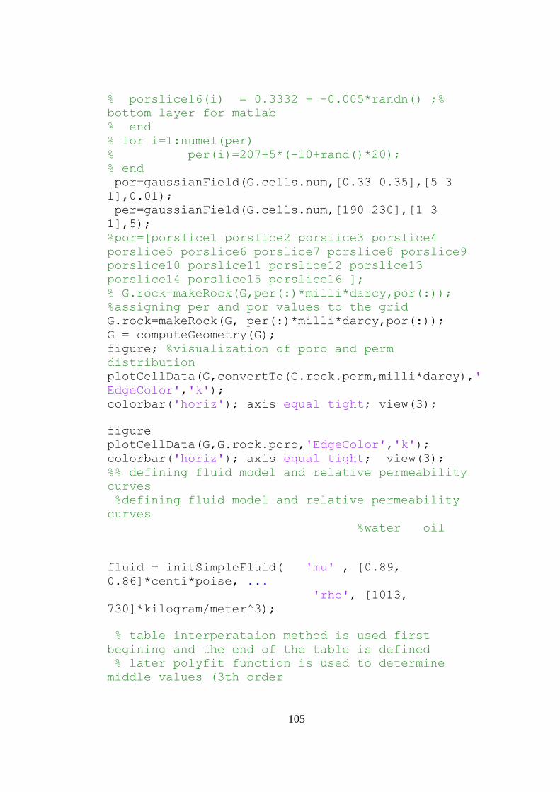
105
% porslice16(i) = 0.3332 + +0.005*randn() ;%
bottom layer for matlab
% end
% for i=1:numel(per)
% per(i)=207+5*(-10+rand()*20);
% end
por=gaussianField(G.cells.num,[0.33 0.35],[5 3
1],0.01);
per=gaussianField(G.cells.num,[190 230],[1 3
1],5);
%por=[porslice1 porslice2 porslice3 porslice4
porslice5 porslice6 porslice7 porslice8 porslice9
porslice10 porslice11 porslice12 porslice13
porslice14 porslice15 porslice16 ];
% G.rock=makeRock(G,per(:)*milli*darcy,por(:));
%assigning per and por values to the grid
G.rock=makeRock(G, per(:)*milli*darcy,por(:));
G = computeGeometry(G);
figure; %visualization of poro and perm
distribution
plotCellData(G,convertTo(G.rock.perm,milli*darcy),'
EdgeColor','k');
colorbar('horiz'); axis equal tight; view(3);
figure
plotCellData(G,G.rock.poro,'EdgeColor','k');
colorbar('horiz'); axis equal tight; view(3);
%% defining fluid model and relative permeability
curves
%defining fluid model and relative permeability
curves
%water oil
fluid = initSimpleFluid( 'mu' , [0.89,
0.86]*centi*poise, ...
'rho', [1013,
730]*kilogram/meter^3);
% table interperataion method is used first
begining and the end of the table is defined
% later polyfit function is used to determine
middle values (3th order
106
% polyfit) finally table interperetation function
is used to linearly
% interpolate between table defined values
% Sw krw
tablebegwat = [
0 0
0.05 0
0.1 0
0.15 0
0.2 0
0.25 0
0.30 0
0.35 0
0.40 0
];
tableendwat=[
0.75 0.8
0.77 0.8
0.8 0.8
0.85 0.8
0.9 0.8
0.95 0.8
1 0.8
];
xx=[0.7499 0.7490 0.40001 0.40007 ]; %water
saturation
zz=[0.7999 0.7990 0.00001 0.00002 ]; %water
relative perm
z=polyfit(xx,zz,3); %function to get wat relative
perm
x1=linspace(0.40001, 0.7499,100);
z1=polyval(z,x1); %getting wat rel perm points for
linearly spaced Sw
tablemid(:,1)=x1; %definig middle table wat sat
points
tablemid(:,2)=z1; %definig middle table krw
table=[tablebegwat; tablemid; tableendwat];
%merging table
107
fluid.krW = @(S) interpTable(table(:, 1), table(:,
2), S); %linear interpolation and combining fluid
object
% So kro
tablebegoil = [
0 0
0.05 0
0.1 0
0.15 0
0.2 0
0.25 0
];
tableendoil=[
0.60 0.14
0.65 0.14
0.70 0.14
0.75 0.14
0.8 0.14
0.85 0.14
0.9 0.14
0.95 0.14
1 0.14
];
xxx=[0.5999 0.5990 0.25001 0.25007 ]; %water
saturation
zzz=[0.1399 0.1390 0.00001 0.00002 ]; %oil rel perm
y=polyfit(xxx,zzz,3); %function to get wat
relative perm
y1=linspace(0.25001, 0.5999,100);
zz1=polyval(y,y1); %getting wat rel perm points for
linearly spaced Sw
tablemidoil(:,1)=y1; %definig middle table wat sat
points
tablemidoil(:,2)=zz1; %definig middle table krw
tableoil=[tablebegoil; tablemidoil; tableendoil];
%merging table
fluid.krO = @(S) interpTable(tableoil(:, 1),
tableoil(:, 2), S); %linear interpolation and
combining fluid object
108
%Sw Pc
table2= [
0.27 20
0.2725 18
0.275 14
0.28 8
0.29 4.04
0.31 3.76
0.33 3.69
0.35 3.62
0.37 3.55
0.39 3.48
0.41 3.41
0.43 3.34
0.45 3.27
0.47 3.2
0.49 3.13
0.51 3.06
0.53 2.99
0.55 2.92
0.57 2.85
0.59 2.78
0.61 2.71
0.63 2.64
0.65 2.57
0.67 2.5
0.69 2.43
0.71 2.25
0.7225 0.20
0.725 0.15
0.7275 0.10
0.73 0.05
];
%fluid.pcOW= @(S)
0.00075*barsa*(interpTable(table2(:,1),table2(:,2),
S));
%fluid.pcOW= @(S) 0;
%plotting rel perm curves
s=linspace(0,1,100);
109
wat=fluid.krW(s);
oil=fluid.krO(s);
%pc = fluid.pcOW(s);
figure
plot(s,wat)
hold on
plot(1-s,oil)
%figure
% plot(s, pc); legend('P_c(S)');
%%
% swaterslice1 =
gaussianField(G.cells.num/16,[0.52 0.54],[1 1
1],0.01) ;%53
% swaterslice2 =
gaussianField(G.cells.num/16,[0.45 0.47],[1 1
1],0.01);%46
% swaterslice3 =
gaussianField(G.cells.num/16,[0.60 0.62],[1 1
1],0.01);%61
% swaterslice4 =
gaussianField(G.cells.num/16,[0.61 0.63],[1 1
1],0.01);%62
% swaterslice5 =
gaussianField(G.cells.num/16,[0.54 0.56],[1 1
1],0.01);%55
% swaterslice6 =
gaussianField(G.cells.num/16,[0.46 0.48],[1 1
1],0.01);%47
% swaterslice7 =
gaussianField(G.cells.num/16,[0.50 0.52],[1 1
1],0.01);%51
% swaterslice8 =
gaussianField(G.cells.num/16,[0.44 0.46],[1 1
1],0.01);%45
% swaterslice9 =
gaussianField(G.cells.num/16,[0.53 0.55],[1 1
1],0.01);%54
% swaterslice10 =
gaussianField(G.cells.num/16,[0.55 0.57],[1 1
1],0.01);%56
110
% swaterslice11 =
gaussianField(G.cells.num/16,[0.52 0.54],[1 1
1],0.01);%53
% swaterslice12 =
gaussianField(G.cells.num/16,[0.50 0.52],[1 1
1],0.01);%51
% swaterslice13 =
gaussianField(G.cells.num/16,[0.45 0.47],[1 1
1],0.01);%46
% swaterslice14 =
gaussianField(G.cells.num/16,[0.47 0.49],[1 1
1],0.01);%48
% swaterslice15 =
gaussianField(G.cells.num/16,[0.60 0.62],[1 1
1],0.01); %61
% swaterslice16 =
gaussianField(G.cells.num/16,[0.52 0.54],[1 1
1],0.01); %53
% Sw=[swaterslice1 swaterslice2 swaterslice3
swaterslice4 swaterslice5 swaterslice6 swaterslice7
swaterslice8 swaterslice9 swaterslice10
swaterslice11 swaterslice12 swaterslice13
swaterslice14 swaterslice15 swaterslice16 ];
% Sw=0.5362*ones(1,G.cells.num);
Sw = gaussianField(G.cells.num,[0.52 0.53],[1 1
1],0.01); %53
So=1-Sw; %oil saturation
%Sw= 0*ones(1,G.cells.num);
%So=1-Sw; %oil saturation
s0 = [Sw', So']; %combining saturation arrays
gravity on %gravity effect
model = TwoPhaseOilWaterModel(G, G.rock, fluid);
%model definitation
%model.operators = TPFAoperators; %model operators
state0 = initResSol(G, 0*barsa, s0); %phase 1 water
2 oil initial state
pv = sum(poreVolume(G, G.rock)); %pore volume of
rock
111
initialoilvolume=sum(poreVolume(G,G.rock).*state0.s
(:,2));
injRate=pv*2/20200; %injection rate m^3/sec
%boundary conditions
bc = fluxside([], G, 'BOTTOM', injRate, 'sat', [1,
0]); %constant flow boundary at the bottom
bc = pside(bc, G, 'TOP', 0.1*barsa, 'sat', [0, 1]);
%constant pressure boundary at the top
n = 100; %step
dT = (20200/n);
states = cell(n+1, 1);
states{1} = state0;
solver.verbose = true;
%% simulation and plotting
schedule = simpleSchedule(repmat(dT,1,n), 'bc',
bc);
[~,sstates] = simulateScheduleAD(state0, model,
schedule);
%%
figure
plotToolbar(G, sstates, 'field',
's:1','lockCaxis',true,'EdgeColor','k'),
colorbar('horiz')
view(30,45);
axis tight equal off
title('Water Saturation Distribution of Core
Plug#2 During 2 PV Water Injection')
caxis([0.20 0.8]);
figure
plotToolbar(G, sstates, 'field',
's:2','lockCaxis',true,'EdgeColor','k'),
colorbar('horiz')
view(30,45);
axis tight equal off
title('Oil Saturation Distribution of Core Plug#2
During 2 PV Water Injection')
caxis([0.20 0.8]);
%% Comparing Exp and Sim Results for Sw
steps=numel(sstates);
112
finalwatsat=sstates{steps,1}.s(:,1);
finalwatsat=reshape(finalwatsat,G.cells.num/celldim
(3),[]);
%finalwatsatperslice(1) =
mean(finalwatsat(1:numel(porslice1)));
for i=1:16
finalwatsatperslice(i) =
mean(finalwatsat(:,i));
end
finalwatsatperslice=fliplr(finalwatsatperslice);
mean(finalwatsatperslice)
finalwatsatperslice(1)=[];
finalwatsatperslice(15)=[];
expxaxis=[ 2 3 4 5 6 7 8 9 10 11 12 13 14 15 ];
swaterexp=[
0.80
0.68
0.60
0.65
0.66
0.68
0.66
0.61
0.61
0.58
0.66
0.68
0.73
0.63
];
%swaterexp=fliplr(swaterexp);
figure
hold on
plot(expxaxis,finalwatsatperslice,'-r*',...
'LineWidth',1,...
'MarkerSize',5)
ylim([0,1])
xlim([1,16])
scatter(expxaxis,swaterexp,'filled')
title('Water Saturation Along the Core Sample')
legend('Simulation Water Saturation','Experimental
Water Saturation')
113
%% Comparing Exp and Sim Results for Recovery
%Comparing Exp and Sim Results for Recovery
voil=ones(1,steps);
vwater=ones(1,steps);
oilvolume=ones(1,steps);
for i=1:100
oilvolume(i)=sum(sstates{i,1}.s(:,2).*poreVolume(G,
G.rock));
end
%%
%voilin=sum(So*pv); %initial oil volume
oilvolume=[initialoilvolume oilvolume];
timee=linspace(0,5.62,numel(oilvolume));
rec=(oilvolume(1)-oilvolume)/oilvolume(1)*100;
bu=linspace(0,20200,101);
injvol=injRate*bu;
oooo=(injvol/sum(pv));
tme=[0.00
0.03
0.32
0.54
1.25
2.42
3.42
4.40
4.90
5.45
5.62
];
recovery =100*[ 0
0.01
0.1
0.11
0.17
0.21
0.25
0.28
0.32
0.3666
0.3666
];
114
figure
hold on
plot(timee,rec,'-r*',...
'LineWidth',1,...
'MarkerSize',5)
ylim([0 100])
scatter(tme,recovery,'filled')
% yyaxis right
% plot(timee,oooo,'-b*',...
% 'LineWidth',1,...
% 'MarkerSize',5)
title('Recovery vs Time and PV injected vs Time')
legend('Simulation Recovery','Experimental
Recovery')
max(rec)
%%
fig1 = figure('Position',[100,100,1200,600]);
fig1.Color = 'w';
colormap('jet');
for i=10: 10: 100
expxaxis=1:celldim(3);
figure(fig1)
SWF=reshape(sstates{i,1}.s(:,1),G.cells.num/celldim
(3),[]);
%plot(expxaxis,swaterexp,'LineWidth',3.0)
%SWF(numel(SWF)/25*25:numel(SWF))=[];
for k=1:celldim(3)
oak(k) = mean(SWF(:,k));
end
oak=fliplr(oak);
hold on
plot(expxaxis,oak,
'LineWidth',1.0,'Color',rand(1,3));
set(gca,'FontSize',15);
xlabel('x')
ylabel('Swf [-]')
ylim([0.0,1.0])
end
%%
for i=1:numel(sstates)
115
pressurebottom(i)=mean(sstates{i,1}.pressure(1:G.ce
lls.num/16))/barsa;
pressuretop(i)=mean(sstates{i,1}.pressure(G.cells.n
um/16*15:G.cells.num))/barsa;
end
deltap=pressuretop-pressurebottom;
timee2=linspace(0,5.62,numel(deltap));
figure
plot(timee2,deltap);
hold on
plot(timee2,ones(1,numel(timee2))*0.02);
Core Plug#7
clc
clear all
close all
%% Load necessary modules
mrstModule add hfm; % hybrid fracture
module
mrstModule add coarsegrid; % functionality for
coarse grids
mrstModule add ad-core; % NNC support for
coarse grids
mrstModule add msrsb; % MsRSB solvers
mrstModule add mrst-gui; % plotting routines
mrstModule add incomp; % Incompressible
fluid models
mrstModule add ad-blackoil; % AD blackoil
solver
mrstModule add ad-core; % AD core module
mrstModule add ad-props; % AD properties
%% Set up a matrix grid
% First set a rectangular(3D) grid and remove cells
to obtain an
% a grid that represents the core plug in 3D
116
celldim = [41, 41, 16]; %number of cellls in x-y-z
directions
physdim = [0.035 0.035 0.074]; % physical dimesions
of the core plug
G = cartGrid(celldim, physdim); %creating the 3D
grid
figure;
plotGrid(G,'EdgeColor','k'); %visualization
axis tight equal
view(3);
G = computeGeometry(G); % geometry computation of
the grid block
x0=0.0175;% x and y coordinates of the circle
y0=0.0175;
radius=0.0175;%radius of circle
c=G.cells.centroids; % Cells centroids in x-y plane
r = (c(:,1)-x0).^2 + (c(:,2)-y0).^2; %defining core
boundary
r=abs(r);
r=sqrt(r);
G = removeCells(G, (r>radius)); %removing cells
G = computeGeometry(G); %computing the geometry
again
figure; %visualization
plotGrid(G,'EdgeColor','k');
view(3);
axis tight equal
% next step is populating the grid with poro and
perm values
por=ones(1,G.cells.num); %poro array
per=ones(1,G.cells.num); %perm array
% for i=1:(G.cells.num/16)
% porslice1(i) = 0.3214 + +0.005*randn() ; %top
layer for matlab
% porslice2(i) = 0.3384 + +0.005*randn() ; %
second layer for matlab value= 15th layer in thesis
% porslice3(i) = 0.3227 + +0.005*randn() ;
% porslice4(i) = 0.3200 + +0.005*randn() ;
% porslice5(i) = 0.3213 + +0.005*randn() ;
% porslice6(i) = 0.3298 + +0.005*randn() ;
117
% porslice7(i) = 0.3269 + +0.005*randn() ;
% porslice8(i) = 0.3175 + +0.005*randn() ;
% porslice9(i) = 0.3209 + +0.005*randn() ;
% porslice10(i) = 0.3160 + +0.005*randn() ;
% porslice11(i) = 0.3109 + +0.005*randn() ;
% porslice12(i) = 0.3228 + +0.005*randn() ;
% porslice13(i) = 0.3240 + +0.005*randn() ;
% porslice14(i) = 0.3209 + +0.005*randn() ;
% porslice15(i) = 0.3145 + +0.005*randn() ;
% porslice16(i) = 0.3214 + +0.005*randn() ;%
bottom layer for matlab
% end
% for i=1:numel(per)
% per(i)=116+5*(-10+rand()*20);
% end
%por=[porslice1 porslice2 porslice3 porslice4
porslice5 porslice6 porslice7 porslice8 porslice9
porslice10 porslice11 porslice12 porslice13
porslice14 porslice15 porslice16 ];
%por=gaussianField(G.cells.num,[0.30 0.35], [5 3
1],0.01);
por=0.32*ones(1,G.cells.num,1);
per=gaussianField(G.cells.num,[110 120], [1 3
5],1);
G.rock=makeRock(G,per(:)*milli*darcy,por(:));
%assigning per and por values to the grid
G = computeGeometry(G);
figure; %visualization of poro and perm
distribution
plotCellData(G,convertTo(G.rock.perm,milli*darcy),'
EdgeColor','k');
colorbar('horiz'); axis equal tight; view(3);
figure
plotCellData(G,G.rock.poro,'EdgeColor','k');
colorbar('horiz'); axis equal tight; view(3);
Gs=G; %creating dublacated G matrix
Gs = computeGeometry(Gs); %computing the geometry
of Gs
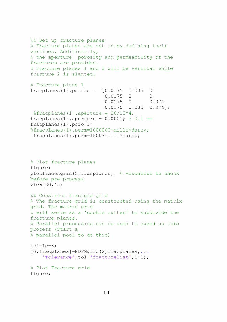
118
%% Set up fracture planes
% Fracture planes are set up by defining their
vertices. Additionally,
% the aperture, porosity and permeability of the
fractures are provided.
% Fracture planes 1 and 3 will be vertical while
fracture 2 is slanted.
% Fracture plane 1
fracplanes(1).points = [0.0175 0.035 0
0.0175 0 0
0.0175 0 0.074
0.0175 0.035 0.074];
%fracplanes(1).aperture = 20/10^4;
fracplanes(1).aperture = 0.0001; % 0.1 mm
fracplanes(1).poro=1;
%fracplanes(1).perm=1000000*milli*darcy;
fracplanes(1).perm=1500*milli*darcy;
% Plot fracture planes
figure;
plotfracongrid(G,fracplanes); % visualize to check
before pre-process
view(30,45)
%% Construct fracture grid
% The fracture grid is constructed using the matrix
grid. The matrix grid
% will serve as a 'cookie cutter' to subdivide the
fracture planes.
% Parallel processing can be used to speed up this
process (Start a
% parallel pool to do this).
tol=1e-8;
[G,fracplanes]=EDFMgrid(G,fracplanes,...
'Tolerance',tol,'fracturelist',1:1);
% Plot Fracture grid
figure;
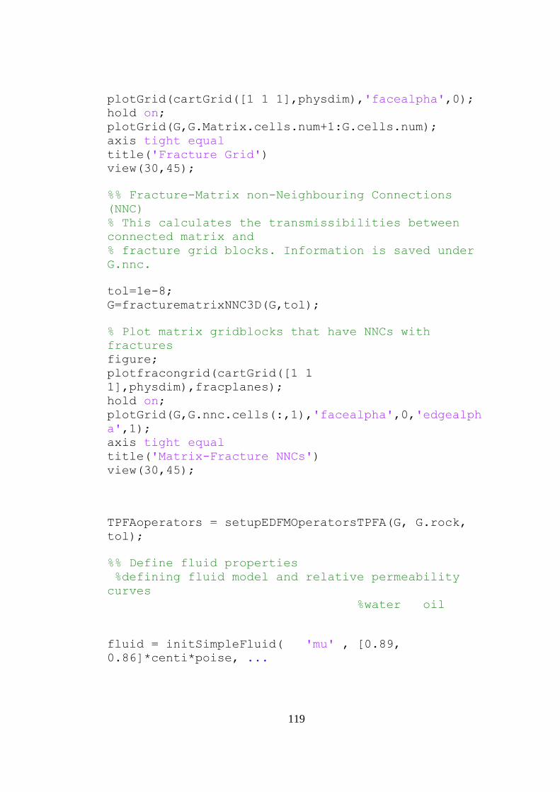
119
plotGrid(cartGrid([1 1 1],physdim),'facealpha',0);
hold on;
plotGrid(G,G.Matrix.cells.num+1:G.cells.num);
axis tight equal
title('Fracture Grid')
view(30,45);
%% Fracture-Matrix non-Neighbouring Connections
(NNC)
% This calculates the transmissibilities between
connected matrix and
% fracture grid blocks. Information is saved under
G.nnc.
tol=1e-8;
G=fracturematrixNNC3D(G,tol);
% Plot matrix gridblocks that have NNCs with
fractures
figure;
plotfracongrid(cartGrid([1 1
1],physdim),fracplanes);
hold on;
plotGrid(G,G.nnc.cells(:,1),'facealpha',0,'edgealph
a',1);
axis tight equal
title('Matrix-Fracture NNCs')
view(30,45);
TPFAoperators = setupEDFMOperatorsTPFA(G, G.rock,
tol);
%% Define fluid properties
%defining fluid model and relative permeability
curves
%water oil
fluid = initSimpleFluid( 'mu' , [0.89,
0.86]*centi*poise, ...
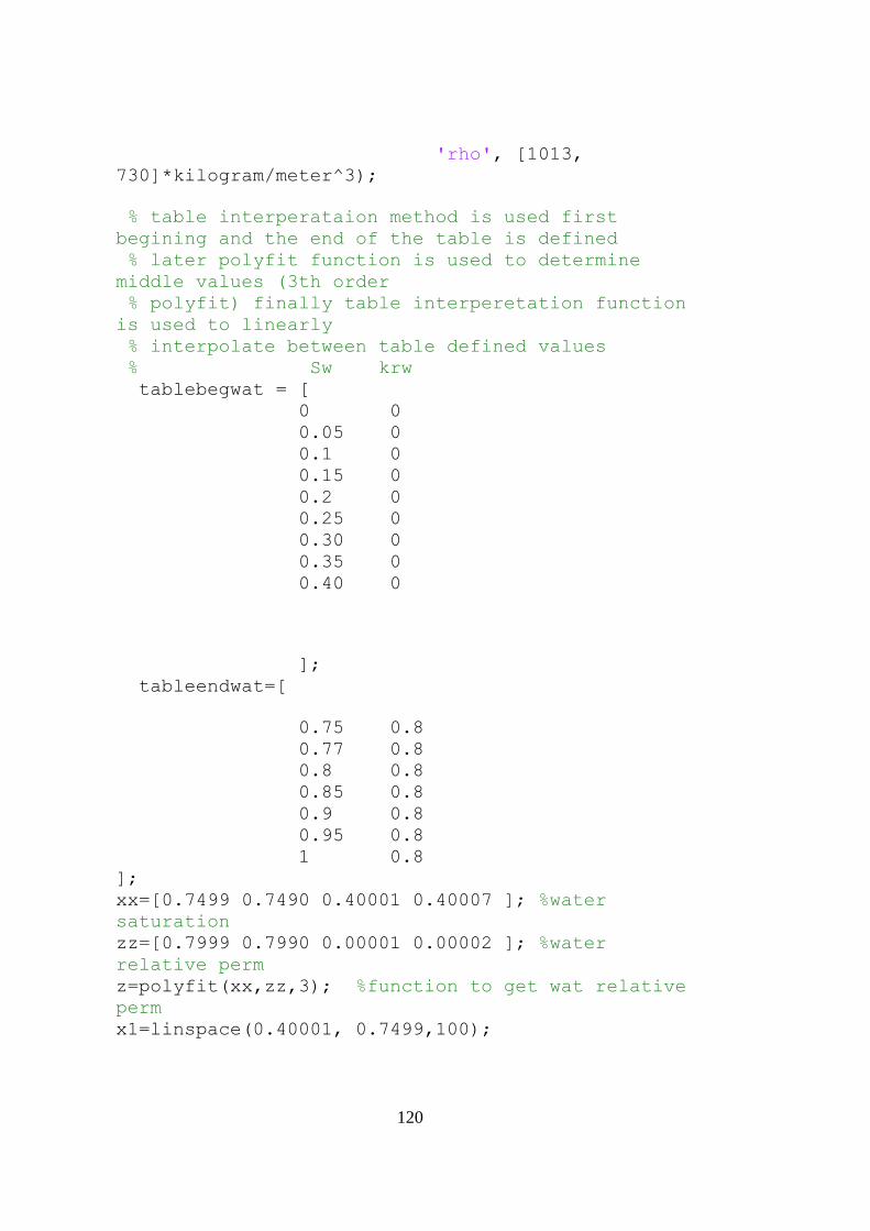
120
'rho', [1013,
730]*kilogram/meter^3);
% table interperataion method is used first
begining and the end of the table is defined
% later polyfit function is used to determine
middle values (3th order
% polyfit) finally table interperetation function
is used to linearly
% interpolate between table defined values
% Sw krw
tablebegwat = [
0 0
0.05 0
0.1 0
0.15 0
0.2 0
0.25 0
0.30 0
0.35 0
0.40 0
];
tableendwat=[
0.75 0.8
0.77 0.8
0.8 0.8
0.85 0.8
0.9 0.8
0.95 0.8
1 0.8
];
xx=[0.7499 0.7490 0.40001 0.40007 ]; %water
saturation
zz=[0.7999 0.7990 0.00001 0.00002 ]; %water
relative perm
z=polyfit(xx,zz,3); %function to get wat relative
perm
x1=linspace(0.40001, 0.7499,100);
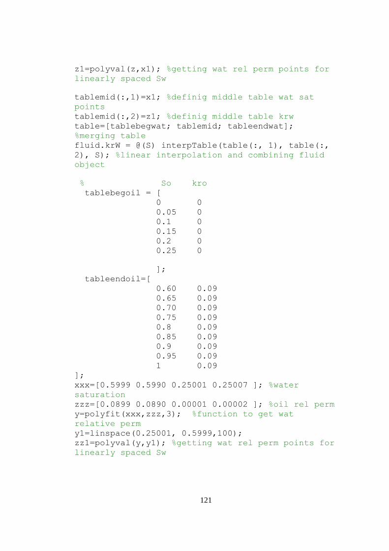
121
z1=polyval(z,x1); %getting wat rel perm points for
linearly spaced Sw
tablemid(:,1)=x1; %definig middle table wat sat
points
tablemid(:,2)=z1; %definig middle table krw
table=[tablebegwat; tablemid; tableendwat];
%merging table
fluid.krW = @(S) interpTable(table(:, 1), table(:,
2), S); %linear interpolation and combining fluid
object
% So kro
tablebegoil = [
0 0
0.05 0
0.1 0
0.15 0
0.2 0
0.25 0
];
tableendoil=[
0.60 0.09
0.65 0.09
0.70 0.09
0.75 0.09
0.8 0.09
0.85 0.09
0.9 0.09
0.95 0.09
1 0.09
];
xxx=[0.5999 0.5990 0.25001 0.25007 ]; %water
saturation
zzz=[0.0899 0.0890 0.00001 0.00002 ]; %oil rel perm
y=polyfit(xxx,zzz,3); %function to get wat
relative perm
y1=linspace(0.25001, 0.5999,100);
zz1=polyval(y,y1); %getting wat rel perm points for
linearly spaced Sw
122
tablemidoil(:,1)=y1; %definig middle table wat sat
points
tablemidoil(:,2)=zz1; %definig middle table krw
tableoil=[tablebegoil; tablemidoil; tableendoil];
%merging table
fluid.krO = @(S) interpTable(tableoil(:, 1),
tableoil(:, 2), S); %linear interpolation and
combining fluid object
%Sw Pc
table2= [
0.27 20
0.2725 18
0.275 14
0.28 8
0.29 4.04
0.31 3.76
0.33 3.69
0.35 3.62
0.37 3.55
0.39 3.48
0.41 3.41
0.43 3.34
0.45 3.27
0.47 3.2
0.49 3.13
0.51 3.06
0.53 2.99
0.55 2.92
0.57 2.85
0.59 2.78
0.61 2.71
0.63 2.64
0.65 2.57
0.67 2.5
0.69 2.43
0.71 2.25
0.7225 0.20
0.725 0.15
0.7275 0.10
0.73 0.05
123
];
%fluid.pcOW= @(S)
0.00075*barsa*(interpTable(table2(:,1),table2(:,2),
S));
%fluid.pcOW= @(S) 0;
%plotting rel perm curves
s=linspace(0,1,100);
wat=fluid.krW(s);
oil=fluid.krO(s);
%pc = fluid.pcOW(s);
figure
plot(s,wat)
hold on
plot(1-s,oil)
%figure
% plot(s, pc); legend('P_c(S)');
%%
% for i=1:(G.cells.num/16)
% swaterslice1(i)=0.41 + 0.005*randn(); %top layer
for matlab
% swaterslice2(i)=0.51 + 0.005*randn(); % second
layer for matlab value= 15th layer in thesis
% swaterslice3(i)=0.50 + 0.005*randn();
% swaterslice4(i)=0.43 + 0.005*randn();
% swaterslice5(i)=0.50 + 0.005*randn();
% swaterslice6(i)=0.51 + 0.005*randn();
% swaterslice7(i)=0.38 + 0.005*randn();
% swaterslice8(i)=0.40 + 0.005*randn();
% swaterslice9(i)=0.35 + 0.005*randn();
% swaterslice10(i)=0.44 + 0.005*randn();
% swaterslice11(i)=0.39 + 0.005*randn();
% swaterslice12(i)=0.34 + 0.005*randn();
% swaterslice13(i)=0.38 + 0.005*randn();
% swaterslice14(i)=0.22 + 0.005*randn();
% swaterslice15(i)=0.40 + 0.005*randn();
% swaterslice16(i)= 0.41+ 0.005*randn();% bottom
layer for matlab
% end
%Sw=[swaterslice1 swaterslice2 swaterslice3
swaterslice4 swaterslice5 swaterslice6 swaterslice7
124
swaterslice8 swaterslice9 swaterslice10
swaterslice11 swaterslice12 swaterslice13
swaterslice14 swaterslice15 swaterslice16 ];
Sw= gaussianField(G.cells.num,[0.41 0.42],[1 3
1],0.001);
So=1-Sw; %oil saturation
s0 = [Sw', So']; %combining saturation arrays
%% Define three-phase compressible flow model
% We define a two-phase black-oil model without
dissolved gas or vaporized
% oil. This is done by first instantiating the
blackoil model, and then
% manually passing in the internal
transmissibilities and the topological
% neighborship from the embedded fracture grid.
gravity on
model = TwoPhaseOilWaterModel(G, G.rock, fluid);
%state0 = initResSol(G, 0*barsa, [Swater, Soil]);
model.operators = TPFAoperators;
state0 = initResSol(G, 0*barsa, s0);
figure
plotToolbar(G, state0, 'field',
's:1','EdgeColor','k'),
view(30,45)
axis tight equal off
colorbar
initialoilvolume=sum(poreVolume(G,G.rock).*state0.s
(:,2))
POREVOLUME=sum(poreVolume(G.Matrix, G.Matrix.rock))
%pv = sum(poreVolume(G, G.rock)); %pore volume of
rock
%injVol=pv*1.08;
%injRate=injVol/11300;
injRate=POREVOLUME/10500;%injection rate m^3/sec
%injRate=0.2*1.667*10^-8;
%boundary conditions
125
bc = fluxside([], G, 'BOTTOM', injRate, 'sat', [1,
0]);
bc = pside(bc, G, 'TOP', 0.06*barsa, 'sat', [0,
1]);
n = 100;
dT = (10500/n);
states = cell(n+1, 1);
states{1} = state0;
solver.verbose = true;
%% Repeat simulation with general solver
% To use the general solver, we first need to set
up a schedule that
% describes the time steps and the drive mechanisms
(wells, boundary
% conditions, and source terms) that are active in
each time step. In
% addition, one can specify various forms of time-
step control. Here,
% however, we simply rely on the default setup
schedule = simpleSchedule(repmat(dT,1,n), 'bc',
bc);
[~,sstates] = simulateScheduleAD(state0, model,
schedule);
%%
figure
plotToolbar(G, sstates, 'field',
's:1','lockCaxis',true,'EdgeColor','k'),
caxis([0.2 0.8]);
title({'Water Saturation Distribution of Core
Plug#7';'During 2 PV Water Injection (Before Gel
Treatment)'})
view(30,45);
axis tight equal
colorbar
figure
plotToolbar(G, sstates, 'field',
's:2','lockCaxis',true,'EdgeColor','k'),
caxis([0.2 0.8]);
126
title({'Water Saturation Distribution of Core
Plug#7';'During 2 PV Water Injection (Before Gel
Treatment)'})
view(30,45);
axis tight equal
colorbar
%%
steps=numel(sstates);
finalwatsat=sstates{steps,1}.s(:,1);
finalwatsatmatrix=finalwatsat(1:G.Matrix.cells.num)
;
FWSM=reshape(finalwatsatmatrix,G.Matrix.cells.num/c
elldim(3),[]);
finalwatsatfracture=finalwatsat(1+G.Matrix.cells.nu
m:G.cells.num);
FWSF=reshape(finalwatsatfracture,G.FracGrid.Frac1.c
ells.num/celldim(3),[]);
%%
%finalwatsatperslice(1) =
mean(finalwatsat(1:numel(por)/16));
for i=1:celldim(3)
%finalwatsatperslice(i) =
mean(finalwatsat(numel(por)/16*(i-
1):i*numel(por)/16));
finalwatsatperslice(i)= mean(FWSM(:,i));
fracfinalwatsatperslice(i)=mean(FWSF(:,i));
corefinalwatsat=[FWSM(:,i)' FWSF(:,i)'];
finalwatsatcore(i)=mean(corefinalwatsat);
end
finalwatsatperslice=fliplr(finalwatsatperslice);
fracfinalwatsatperslice=fliplr(fracfinalwatsatpersl
ice);
finalwatsatcore=fliplr(finalwatsatcore);
%%
mean(finalwatsatperslice)
finalwatsatperslice(1)=[];
finalwatsatperslice(15)=[];
finalwatsatcore(1)=[];
finalwatsatcore(15)=[];
fracfinalwatsatperslice(1)=[];
fracfinalwatsatperslice(15)=[];
expxaxis=[ 2 3 4 5 6 7 8 9 10 11 12 13 14 15];
127
swaterexp=[ 1.00
0.74
0.62
0.88
0.64
0.48
0.46
0.70
0.30
0.44
0.50
0.45
0.44
0.45];
figure
hold on
plot(expxaxis,finalwatsatperslice,'-r*',...
'LineWidth',1,...
'MarkerSize',5)
ylim([0.,1])
plot(expxaxis,finalwatsatcore,'-b*',...
'LineWidth',1,...
'MarkerSize',5)
plot(expxaxis,fracfinalwatsatperslice,'-g*',...
'LineWidth',1,...
'MarkerSize',5)
scatter(expxaxis,swaterexp,'filled')
title('Water Saturation Along the Core Sample')
legend('Matrix Water Saturation','Overalll Core
Water Saturation','Fracture Water Saturation','Exp
Water Saturation')
ylim([0,1])
xlim([1,16])
%%
%%Comparing Exp and Sim Results for Recovery
voil=ones(1,steps);
vwater=ones(1,steps);
%oilvolume=ones(1,steps);
for i=1:100
128
oilvolume(i)=sum(sstates{i,1}.s(:,2).*poreVolume(G,
G.rock));
end
%%
oilvolume=[initialoilvolume oilvolume];
timee=linspace(0,2.92,numel(oilvolume));
rec=(oilvolume(1)-oilvolume)/oilvolume(1)*100;
bu=linspace(0,10500,101);
injvol=injRate*bu;
%%
tme=[0
0.33
0.5
0.7
1
1.25
1.33
1.5
1.78
2
2.33
2.53
2.63
2.75
2.92
];
recovery =[
0
7
9.5
14
18
21
23
23
25.5
26
27.5
28
28.57
129
28.57
28.57
];
figure
hold on
plot(timee,rec,'-r*',...
'LineWidth',1,...
'MarkerSize',5)
ylim([0 100])
scatter(tme,recovery,'filled')
% yyaxis right
% plot(timee,oooo,'-b*',...
% 'LineWidth',1,...
% 'MarkerSize',5)
title('Recovery vs Time and PV injected vs Time')
legend('Simulation Recovery','Experimental
Recovery')
max(rec)
%%
fig1 = figure('Position',[100,100,1200,600]);
fig1.Color = 'w';
colormap('jet');
eexpxaxis=1:celldim(3);
% swin=0.27*ones(1,16);
% swmax=0.73*ones(1,16);
% plot(expxaxis,swin);
% hold on
% plot(expxaxis,swmax);
for i=1 :10 : 100
figure(fig1)
hold on
%SWF=reshape(sstates{i,1}.s(:,1),G.cells.num/celldi
m(3),[]);
finalwatsat=sstates{i,1}.s(:,1);
finalwatsatmatrix=finalwatsat(1:G.Matrix.cells.num)
;
FWSM=reshape(finalwatsatmatrix,G.Matrix.cells.num/c
elldim(3),[]);
130
finalwatsatfracture=finalwatsat(1+G.Matrix.cells.nu
m:G.cells.num);
FWSF=reshape(finalwatsatfracture,G.FracGrid.Frac1.c
ells.num/celldim(3),[]);
for k=1:celldim(3)
matrixsat(k) = mean(FWSM(:,k));
fracturesat(k) = mean(FWSF(:,k));
end
eexpxaxis=(1:celldim(3));
matrixsat=fliplr(matrixsat);
fracturesat=fliplr(fracturesat);
plot(eexpxaxis,matrixsat,
'LineWidth',1.0,'Color',rand(1,3));
set(gca,'FontSize',16);
xlabel('x')
ylabel('Swf [-]')
title('Water Saturation of Matrix')
ylim([0,1])
end
fig2 = figure('Position',[100,100,1200,600]);
fig2.Color = 'w';
colormap('jet');
for i=1 :10 : 100
figure(fig2)
hold on
%SWF=reshape(sstates{i,1}.s(:,1),G.cells.num/celldi
m(3),[]);
finalwatsat=sstates{i,1}.s(:,1);
finalwatsatmatrix=finalwatsat(1:G.Matrix.cells.num)
;
FWSM=reshape(finalwatsatmatrix,G.Matrix.cells.num/c
elldim(3),[]);
finalwatsatfracture=finalwatsat(1+G.Matrix.cells.nu
m:G.cells.num);
131
FWSF=reshape(finalwatsatfracture,G.FracGrid.Frac1.c
ells.num/celldim(3),[]);
for k=1:celldim(3)
matrixsat(k) = mean(FWSM(:,k));
fracturesat(k) = mean(FWSF(:,k));
end
eexpxaxis=(1:celldim(3));
matrixsat=fliplr(matrixsat);
fracturesat=fliplr(fracturesat);
plot(eexpxaxis,fracturesat,
'LineWidth',1.0,'Color',rand(1,3));
set(gca,'FontSize',16);
xlabel('x')
ylabel('Swf [-]')
title('Water Saturation of Fracture')
ylim([0,1])
end
fig3 = figure('Position',[100,100,1200,600]);
fig3.Color = 'w';
colormap('jet');
for i=1 :10 : 100
figure(fig3)
hold on
%SWF=reshape(sstates{i,1}.s(:,1),G.cells.num/celldi
m(3),[]);
finalwatsat=sstates{i,1}.s(:,1);
finalwatsatmatrix=finalwatsat(1:G.Matrix.cells.num)
;
FWSM=reshape(finalwatsatmatrix,G.Matrix.cells.num/c
elldim(3),[]);
finalwatsatfracture=finalwatsat(1+G.Matrix.cells.nu
m:G.cells.num);
FWSF=reshape(finalwatsatfracture,G.FracGrid.Frac1.c
ells.num/celldim(3),[]);
for i=1:celldim(3)
132
FWSC(:,i)= [FWSM(:,i)',FWSF(:,i)'];
end
for k=1:celldim(3)
matrixsat(k) = mean(FWSM(:,k));
fracturesat(k) = mean(FWSF(:,k));
coresat(k)=mean(FWSC(:,k));
end
eexpxaxis=(1:celldim(3));
matrixsat=fliplr(matrixsat);
fracturesat=fliplr(fracturesat);
coresat=fliplr(coresat);
plot(eexpxaxis,coresat,
'LineWidth',1.0,'Color',rand(1,3));
set(gca,'FontSize',16);
xlabel('x')
ylabel('Swf [-]')
title('Water Saturation of Combined Core')
ylim([0,1])
end
%%
fracplane(1).points = [0.0175 0.035 0
0.0175 0 0
0.0175 0 0.074
0.0175 0.035 0.074];
fracplane(1).aperture = 0.0000250; % 0.25 mm
fracplane(1).poro=1;
fracplane(1).perm=10*milli*darcy;
[Gs,fracplane]=EDFMgrid(Gs,fracplane,...
'Tolerance',tol,'fracturelist',1:1);
Gs=fracturematrixNNC3D(Gs,tol);
TPFAoperators = setupEDFMOperatorsTPFA(Gs, Gs.rock,
tol);
%%
% fluid = initSimpleFluid( 'mu' , [0.89,
0.86]*centi*poise, ...
133
% 'rho', [1013,
860]*kilogram/meter^3, ...
% 'n', [4, 6.3]);
gravity on
model = TwoPhaseOilWaterModel(Gs, Gs.rock, fluid);
%model = OilWaterPolymerModel(Gs, Gs.rock, fluid);
%state0 = initResSol(G, 0*barsa, [Swater, Soil]);
model.operators = TPFAoperators;
state0 = sstates{100,1};
%injRate=0.4*1.6667*10^-8;
injRate=2*POREVOLUME/6600;
bc = fluxside([], Gs, 'BOTTOM', injRate, 'sat', [1,
0]);
bc = pside(bc, Gs, 'TOP', 4*barsa, 'sat', [0, 1]);
n = 100;
dT = (9600/n);
states = cell(n+1, 1);
states{1} = state0;
solver.verbose = true;
schedule = simpleSchedule(repmat(dT,1,n), 'bc',
bc);
[~,sstates] = simulateScheduleAD(state0, model,
schedule);
%%
figure
plotToolbar(Gs, sstates, 'field',
's:1','lockCaxis',true,'EdgeColor','k'),
view(30,45);
axis tight equal
caxis([0.2 0.8]);
title({'Water Saturation Distribution of Core
Plug#7';'During 2 PV Water Injection (After Gel
Treatment)'})
colorbar
figure
plotToolbar(Gs, sstates, 'field',
's:2','lockCaxis',true,'EdgeColor','k'),
view(30,45);
axis tight equal
134
caxis([0.2 0.8]);
title({'Oil Saturation Distribution of Core
Plug#7';'During 2 PV Water Injection (After Gel
Treatment)'})
colorbar
%%
steps=numel(sstates);
finalwatsat=sstates{steps,1}.s(:,1);
finalwatsatmatrix=finalwatsat(1:G.Matrix.cells.num)
;
FWSM=reshape(finalwatsatmatrix,G.Matrix.cells.num/c
elldim(3),[]);
finalwatsatfracture=finalwatsat(1+G.Matrix.cells.nu
m:G.cells.num);
FWSF=reshape(finalwatsatfracture,G.FracGrid.Frac1.c
ells.num/celldim(3),[]);
%%
%finalwatsatperslice(1) =
mean(finalwatsat(1:numel(por)/16));
for i=1:celldim(3)
%finalwatsatperslice(i) =
mean(finalwatsat(numel(por)/16*(i-
1):i*numel(por)/16));
finalwatsatperslice(i)= mean(FWSM(:,i));
fracfinalwatsatperslice(i)=mean(FWSF(:,i));
corefinalwatsat=[FWSM(:,i)' FWSF(:,i)'];
finalwatsatcore(i)=mean(corefinalwatsat);
end
finalwatsatperslice=fliplr(finalwatsatperslice);
fracfinalwatsatperslice=fliplr(fracfinalwatsatpersl
ice);
finalwatsatcore=fliplr(finalwatsatcore);
mean(finalwatsatperslice)
finalwatsatperslice(1)=[];
finalwatsatperslice(15)=[];
finalwatsatcore(1)=[];
finalwatsatcore(15)=[];
fracfinalwatsatperslice(1)=[];
fracfinalwatsatperslice(15)=[];
%%
expxaxis=[ 2 3 4 5 6 7 8 9 10 11 12 13 14 15 ];
135
swaterexp=[ 1.00
0.95
0.89
0.86
0.87
0.65
0.73
0.65
0.73
0.70
0.52
0.52
0.45
0.60];
figure
hold on
plot(expxaxis,finalwatsatperslice,'-r*',...
'LineWidth',1,...
'MarkerSize',5)
ylim([0,1])
xlim([1,16])
scatter(expxaxis,swaterexp,'filled')
title('Water Saturation Along the Core Sample')
legend('Simulation Water Saturation','Experimental
Water Saturation')
%%
%voil=ones(1,steps);
%vwater=ones(1,steps);
%oilvolume=ones(1,steps);
%oilvolume=[initialoilvolume oilvolume];
%timee=linspace(4.33,6.5,numel(oilvolume));
%rec=(oilvolume(1)-oilvolume)/oilvolume(1)*100;
%bu=linspace(0,23400,101);
%injvol=injRate*bu;
% for i=1:100
%
oilvolume2(i)=sum(sstates{i,1}.s(:,2).*poreVolume(G
,G.rock));
% end
tme=[0
136
0.33
0.5
0.7
1
1.25
1.33
1.5
1.78
2
2.33
2.53
2.63
2.75
2.92
4.71
4.88
5.13
5.41
5.53
5.7
6.03
6.36
6.63
6.91
7.08
7.13
];
recovery =[ 0
7
9.5
14
18
21
23
23
25.5
26
27.5
28
28.57
28.57
28.57
137
28.57
32
35
40
41
42.85
42.85
42.85
42.85
42.85
42.85
42.85
];
%%
for i=1:100
% vwateri(i)=
sum(sstates{i,1}.s(:,1).*poreVolume(G,G.rock));
%voili(i)=sum(sstates{i,1}.s(:,2).*poreVolume(G,G.r
ock));
oilvolume2(i)=sum(sstates{i,1}.s(:,2).*poreVolume(G
,G.rock));
end
oilvolume=[oilvolume oilvolume2];
timeee=linspace(4.71,7.23,numel(oilvolume2));
timee=[timee timeee];
rec=(oilvolume(1)-oilvolume)/oilvolume(1)*100;
%%
figure
hold on
plot(timee,rec,'-r*',...
'LineWidth',1,...
'MarkerSize',5)
ylim([0 100])
scatter(tme,recovery,'filled')
title('Recovery vs Time')
legend('Simulation Recovery','Experimental
Recovery')
max(rec)