Simulation of CO2 for Enhanced Oil Recovery2 Olga and Rocx or OLGA is a one-dimensional transient dynamic multiphase simulator used to simulate flow in pipelines and connected equipment

Simulation of CO2 for Enhanced Oil Recovery

Ludmila Vesjolaja Ambrose Ugwu Arash Abbasi Emmanuel Okoye

Britt M. E. Moldestad

Department of Process, Energy and Environmental Technology, University College of Southeast Norway, Norway,[email protected]

AbstractCO2-EOR is one of the main methods for tertiary oil

recovery. The injection of CO2 does not only improve

oil recovery, but also contribute to the mitigation of

greenhouse gas emissions. In this study, near well

simulations were performed to determine the optimum

differential pressure and evaluate the effect of CO2

injection in oil recovery. By varying the drawdown from

3 bar to 20 bar, the most suitable differential pressure

for the simulations was found to be 10 bar. The effect of

CO2 injection on oil recovery was simulated by

adjusting the relative permeability curves using Corey

and STONE II correlations. By decreasing the residual

oil saturation from 0.3 to 0.15 due to CO2 injection, the

oil recovery factor increased from 0.52 to 0.59 and the

water production decreased by 22%.

Keywords: CO2, enhanced oil recovery, relative

permeability, near well simulation

1 Introduction

According to Melzer (2012) and Jelmert et al (2010),

after water flooding CO2-EOR is the most commonly

used method for improved oil recovery. CO2-EOR can

be used for increased oil production in combination with

CO2 storage to mitigate CO2 emissions. The method is

widely used in the United States where the price of CO2

is relatively low due to large resources of natural CO2.

More than 70 operating fields in USA use CO2 for

enhanced oil recovery. The majority of oil fields use

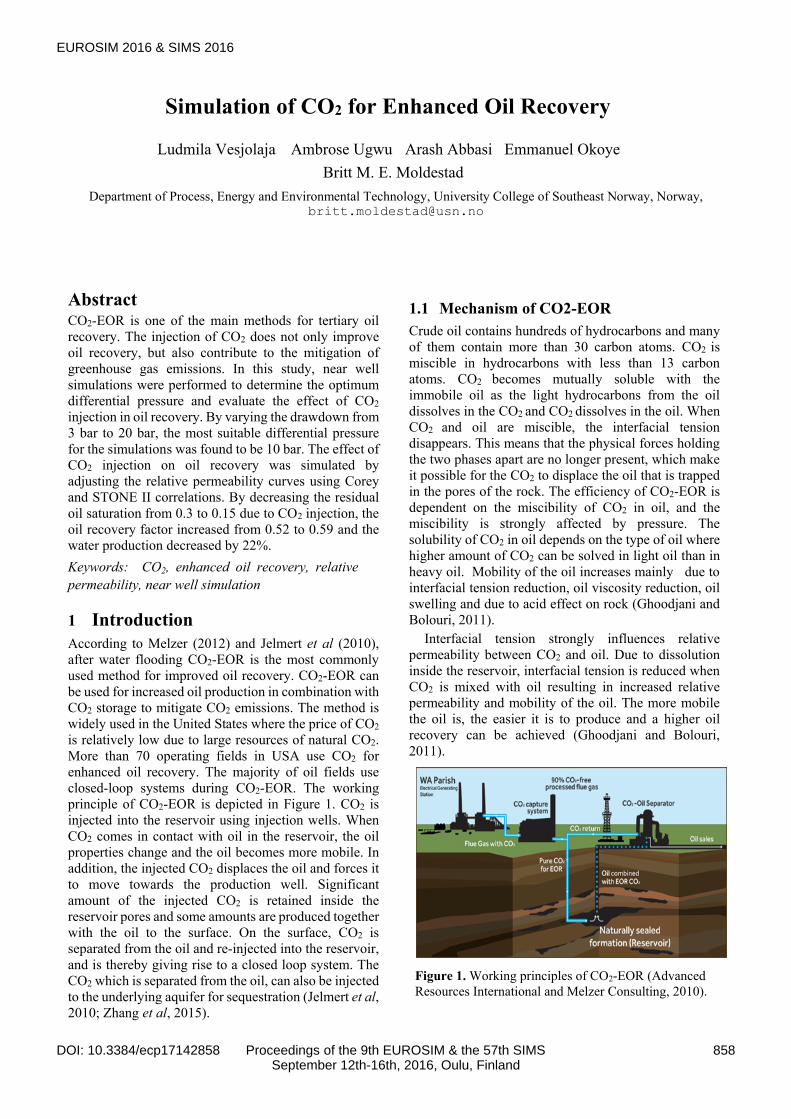
closed-loop systems during CO2-EOR. The working

principle of CO2-EOR is depicted in Figure 1. CO2 is

injected into the reservoir using injection wells. When

CO2 comes in contact with oil in the reservoir, the oil

properties change and the oil becomes more mobile. In

addition, the injected CO2 displaces the oil and forces it

to move towards the production well. Significant

amount of the injected CO2 is retained inside the

reservoir pores and some amounts are produced together

with the oil to the surface. On the surface, CO2 is

separated from the oil and re-injected into the reservoir,

and is thereby giving rise to a closed loop system. The

CO2 which is separated from the oil, can also be injected

to the underlying aquifer for sequestration (Jelmert et al,

2010; Zhang et al, 2015).

1.1 Mechanism of CO2-EOR

Crude oil contains hundreds of hydrocarbons and many

of them contain more than 30 carbon atoms. CO2 is

miscible in hydrocarbons with less than 13 carbon

atoms. CO2 becomes mutually soluble with the

immobile oil as the light hydrocarbons from the oil

dissolves in the CO2 and CO2 dissolves in the oil. When

CO2 and oil are miscible, the interfacial tension

disappears. This means that the physical forces holding

the two phases apart are no longer present, which make

it possible for the CO2 to displace the oil that is trapped

in the pores of the rock. The efficiency of CO2-EOR is

dependent on the miscibility of CO2 in oil, and the

miscibility is strongly affected by pressure. The

solubility of CO2 in oil depends on the type of oil where

higher amount of CO2 can be solved in light oil than in

heavy oil. Mobility of the oil increases mainly due to

interfacial tension reduction, oil viscosity reduction, oil

swelling and due to acid effect on rock (Ghoodjani and

Bolouri, 2011).

Interfacial tension strongly influences relative

permeability between CO2 and oil. Due to dissolution

inside the reservoir, interfacial tension is reduced when

CO2 is mixed with oil resulting in increased relative

permeability and mobility of the oil. The more mobile

the oil is, the easier it is to produce and a higher oil

recovery can be achieved (Ghoodjani and Bolouri,

2011).

Figure 1. Working principles of CO2-EOR (Advanced

Resources International and Melzer Consulting, 2010).

EUROSIM 2016 & SIMS 2016

858DOI: 10.3384/ecp17142858 Proceedings of the 9th EUROSIM & the 57th SIMSSeptember 12th-16th, 2016, Oulu, Finland

1.1 Mechanism of CO2-EOR

Crude oil contains hundreds of hydrocarbons and many

of them contain more than 30 carbon atoms. CO2 is

miscible in hydrocarbons with less than 13 carbon

atoms. CO2 becomes mutually soluble with the

immobile oil as the light hydrocarbons from the oil

dissolves in the CO2 and CO2 dissolves in the oil. When

CO2 and oil are miscible, the interfacial tension

disappears. This means that the physical forces holding

the two phases apart are no longer present, which make

it possible for the CO2 to displace the oil that is trapped

in the pores of the rock. The efficiency of CO2-EOR is

dependent on the miscibility of CO2 in oil, and the

miscibility is strongly affected by pressure. The

solubility of CO2 in oil depends on the type of oil where

higher amount of CO2 can be solved in light oil than in

heavy oil. Mobility of the oil increases mainly due to

interfacial tension reduction, oil viscosity reduction, oil

swelling and due to acid effect on rock (Ghoodjani and

Bolouri, 2011).

Interfacial tension strongly influences relative

permeability between CO2 and oil. Due to dissolution

inside the reservoir, interfacial tension is reduced when

CO2 is mixed with oil resulting in increased relative

permeability and mobility of the oil. The more mobile

the oil is, the easier it is to produce and a higher oil

recovery can be achieved (Ghoodjani and Bolouri,

2011).

Figure 1. Working principles of CO2-EOR (Advanced

Resources International and Melzer Consulting, 2010).

When CO2 dissolves in oil, the viscosity of the oil

decreases significantly. The reduction of oil viscosity is

highly dependent on the initial viscosity of the oil. Less

viscous oil will be less affected by the CO2, while for

more viscous oils, the effect of viscosity reduction is

more pronounced. The reduction in oil viscosity will

cause an increase in the oil relative permeability. This

will reduce the residual oil saturation in the reservoir

and improve the oil recovery (Ghoodjani and Bolouri,

2011).

CO2 interacts with the oil in the reservoir and

dissolves in the oil at certain reservoir conditions. The

dissolution of CO2 in oil causes the oil to swell.

Reservoir characteristics, as pressure and temperature as

well as oil composition, determine the strength of the oil

swelling effect (Ghoodjani and Bolouri, 2011). Swelling

plays an important role in achieving better oil recovery.

Variation in the swelling factor influences on the

residual oil saturation, which is inversely proportional

to the swelling factor. Residual oil saturation, in turn,

affects the relative permeability, which plays a crucial

role in oil recovery (Ghoodjani and Bolouri, 2011).

Swollen oil droplets force fluids to move out of the

pores and oil that initially was unable to move out of the

pores under certain pressure conditions will now be

forced to move towards the production well. Hence, oil

swelling causes drainage effect that decreases the

residual oil saturation (Ghoodjani and Bolouri, 2011).

2 Olga and Rocx

OLGA is a one-dimensional transient dynamic

multiphase simulator used to simulate flow in pipelines

and connected equipment. OLGA consists of several

modules depicting transient flow in a multiphase

pipeline, pipeline networks and processing equipment.

Since Olga is a spatially 1-dimensional simulator, only

one set of equations is used for the calculation of the

well properties in the length direction. That is, the

properties of the fluid are independent of the radius of

the well and changes therefore only with length and time

(Thu, 2013).

Rocx is a three-dimensional near-well model coupled

to the OLGA simulator to perform integrated wellbore-

reservoir transient simulations. Rocx can simulate three-

phase flow in porous media. It has two OLGA PVT

options available, among which black-oil tracking is

used in this project. Rocx simulations can be run without

the coupling to OLGA. However, by using Rocx in

combination with OLGA, more accurate predictions of

well start-up and shut-down, observation of flow

instabilities, cross flow between different layers, water

coning and gas dynamic can be obtained (Schlumberger,

2007). The OLGA simulator is governed by

conservation of mass equations for gas, liquid and liquid

droplets, conservation of momentum equations for the

liquid phase and the liquid droplets at the walls, and

conservation of energy mixture equation with phases

having the same temperature (Schlumberger, 2007).

2.1 Rocx

Schlumberger (2007) describes the mathematical

models used in Rocx in detail. The models for relative

permeability developed by Corey and Stone II are

presented below.

In this study, the Corey model is used to define the

relative permeability curves for water (Li and Horne,

2006; Rocx Online Help). This model is a combination

of the Burdine approach for calculation of the relative

permeability of the wetting and non-wetting phases and

the capillary pressure model that was defined by Corey.

The Corey model is also called the Brooks and Corey

model depending on the value of the pore size

distribution index. If the pore size distribution index is

less than 2, the model is called the Corey model and if it

is greater than 2, it is called the Brooks and Corey model

(Li and Horne, 2006). The Corey model (Rocx Online

Help) for predicting the relative permeability of water is

given by:

krw = krowc (Sw − Swc

1 − Sor − Swc)nw

(1)

where krw is the relative permeability of water, krowc is

the relative permeability of water at the maximum water

saturation, Sw is the water saturation, Swc is the

irreducible water saturation, Sor is the residual oil

saturation and nw is the Corey fitting parameter for

water.

The Stone II model is used in to calculate the relative

permeability of oil. This model is widely used for

predicting relative permeability in water-wetted systems

with high saturations of oil. The Stone II model

estimates the relative permeability of oil in an oil-water

system based on the following equation (Rocx Online

Help):

𝑘𝑟𝑜𝑤 = 𝑘𝑟𝑜𝑤𝑐 (𝑆𝑤 + 𝑆𝑜𝑟 − 1

𝑆𝑤𝑐 + 𝑆𝑜𝑟 − 1)𝑛𝑜𝑤

(2)

where 𝑘𝑟𝑜𝑤 is the relative oil permeability for the water-

oil system, 𝑘𝑟𝑜𝑤𝑐 is the endpoint relative permeability

for oil in water at irreducible water saturation and 𝑛𝑜𝑤 is

a fitting parameter for oil.

3 Simulation Details

This section describes the simulation method and

procedures. A near-well reservoir is constructed in

Rocx, imported to OLGA and simulated. The results are

presented using OLGA and Tecplot.

3.1 Geometry

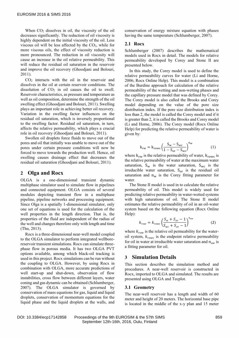
The near-well reservoir has a length and width of 60

meter and height of 20 meters. The horizontal base pipe

is located in the middle of the x-y plan and 15 meter



above the bottom of the reservoir. Figure 2 presents a

schematic overview of the simulated reservoir.

The water drive pressure from the bottom of the

reservoir is 320 bar and the pressure in the base pipe is

varied from 300 to 317 bar. Differential pressures of 3,

5, 10, 15 and 20 bars were used as the driving force for

oil production in the simulation. The pressure at the

outer boundary of the reservoir was constant at 320 bars,

since the reservoir is considered to be infinitely large.

The grid was set to (nx, ny, nz) = (3, 31, 20).

3.2 Reservoir Conditions

Reservoir characteristics were chosen according to the

Grane oil field in the North Sea. Grane was selected for

this research since this is the first field that started to

produce heavy crude oil in Norway (Fath and

Pouranfard, 2014). The reservoir is characterized as

homogeneous reservoir without gas-cap and with high

porosity (0.33) and permeability (up to 10 D). The oil

viscosity at reservoir conditions reaches 12 cP with

19°API gravity.

According to Fath and Pouranfard (2014), MMP for

carbon dioxide and oil (20° API) is 320 bar (at 121 °C).

The reservoir pressure in the Grane field is 176 bar.

However, in order to simulate the miscible CO2-EOR

method, the reservoir pressure was set to 320 bar and the

temperature to 121 °C. The rock is defined as sandstone,

and the thermal properties was chosen from data given

by Eppelbaum et al (2014). The reservoir characteristics

of the Grane field and the reservoir characteristics used

in this study are listed in Table 1.

Figure 2. Schematic overview of the near-well reservoir.

Table 1. Reservoir characteristics of Grane field and the

simulated reservoir.

Parameter Grane field

reservoir

The simulated

reservoir

Oil viscosity 10-12 cp @ 76

°C and 176 bar

12 cp @ 76 °C

and 176 bar

Oil specific

gravity

0.876 (19°

API)

0.876 (19°

API)

Porosity 0.33 0.33

Permeability Up to 10 D

x and y-

directions: 7 D

z-direction

(gravity): 0.7 D

Area 25.5 km2 1860 m2

(60X31)

Thickness 31 m 20 m

Gas Oil Ratio 14-18

Sm3/Sm3 15 Sm3/Sm3

Reservoir

pressure 176 bar 320 bar

Reservoir

temperature 76 °C 121 °C

Rock

compressibility Not found 0.00001 1/bar

Rock heat

conductivity Not found 1.7 W/mK

Rock heat

capacity Not found 737 J/kgK

Rock density Not found 2198 kg/m3

Initial oil

saturation Not found 1

Irreducible

water

saturation

Not found 0.18

Residual oil

saturation Not found

0.3 (before CO2

breakthrough)

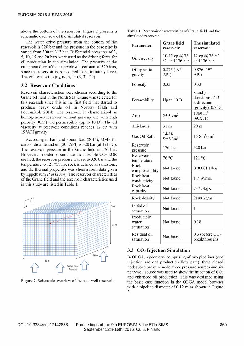
3.3 CO2 Injection Simulation

In OLGA, a geometry comprising of two pipelines (one

injection and one production flow path), three closed

nodes, one pressure node, three pressure sources and six

near-well source was used to show the injection of CO2

and enhanced oil production. This was designed using

the basic case function in the OLGA model browser

with a pipeline diameter of 0.12 m as shown in Figure

3.



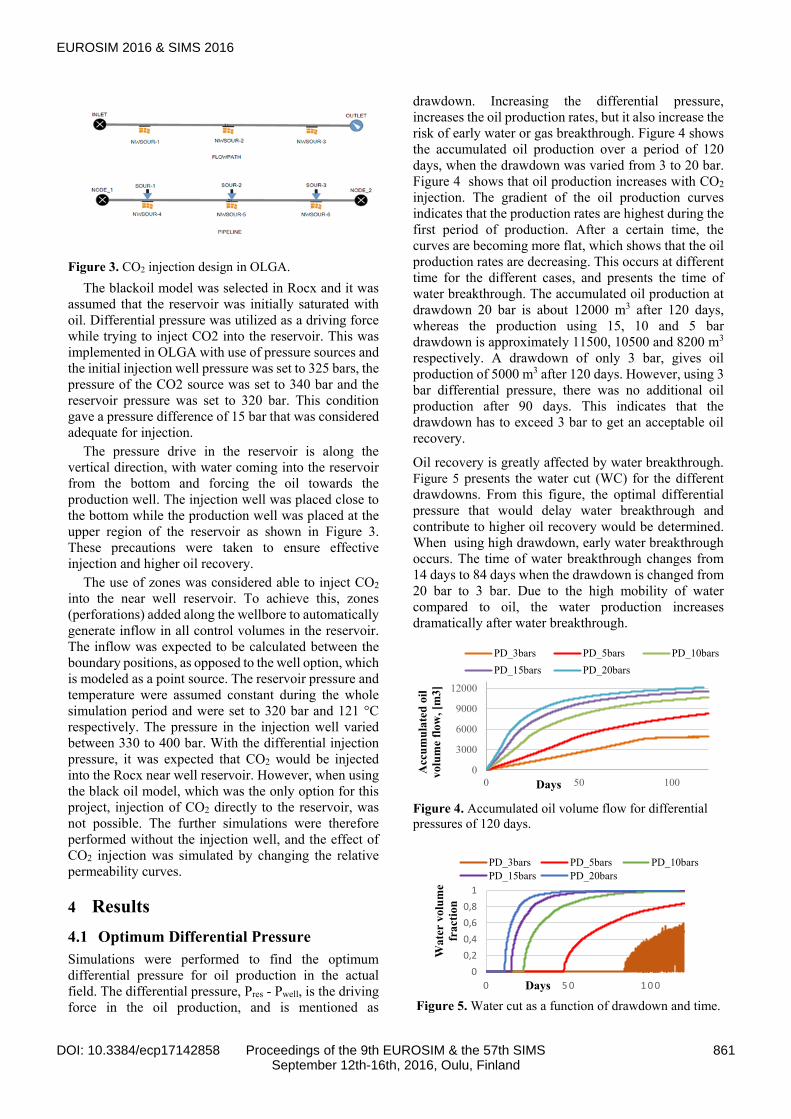
Figure 3. CO2 injection design in OLGA.

The blackoil model was selected in Rocx and it was

assumed that the reservoir was initially saturated with

oil. Differential pressure was utilized as a driving force

while trying to inject CO2 into the reservoir. This was

implemented in OLGA with use of pressure sources and

the initial injection well pressure was set to 325 bars, the

pressure of the CO2 source was set to 340 bar and the

reservoir pressure was set to 320 bar. This condition

gave a pressure difference of 15 bar that was considered

adequate for injection.

The pressure drive in the reservoir is along the

vertical direction, with water coming into the reservoir

from the bottom and forcing the oil towards the

production well. The injection well was placed close to

the bottom while the production well was placed at the

upper region of the reservoir as shown in Figure 3.

These precautions were taken to ensure effective

injection and higher oil recovery.

The use of zones was considered able to inject CO2

into the near well reservoir. To achieve this, zones

(perforations) added along the wellbore to automatically

generate inflow in all control volumes in the reservoir.

The inflow was expected to be calculated between the

boundary positions, as opposed to the well option, which

is modeled as a point source. The reservoir pressure and

temperature were assumed constant during the whole

simulation period and were set to 320 bar and 121 °C

respectively. The pressure in the injection well varied

between 330 to 400 bar. With the differential injection

pressure, it was expected that CO2 would be injected

into the Rocx near well reservoir. However, when using

the black oil model, which was the only option for this

project, injection of CO2 directly to the reservoir, was

not possible. The further simulations were therefore

performed without the injection well, and the effect of

CO2 injection was simulated by changing the relative

permeability curves.

4 Results

4.1 Optimum Differential Pressure

Simulations were performed to find the optimum

differential pressure for oil production in the actual

field. The differential pressure, Pres - Pwell, is the driving

force in the oil production, and is mentioned as

drawdown. Increasing the differential pressure,

increases the oil production rates, but it also increase the

risk of early water or gas breakthrough. Figure 4 shows

the accumulated oil production over a period of 120

days, when the drawdown was varied from 3 to 20 bar.

Figure 4 shows that oil production increases with CO2

injection. The gradient of the oil production curves

indicates that the production rates are highest during the

first period of production. After a certain time, the

curves are becoming more flat, which shows that the oil

production rates are decreasing. This occurs at different

time for the different cases, and presents the time of

water breakthrough. The accumulated oil production at

drawdown 20 bar is about 12000 m3 after 120 days,

whereas the production using 15, 10 and 5 bar

drawdown is approximately 11500, 10500 and 8200 m3

respectively. A drawdown of only 3 bar, gives oil

production of 5000 m3 after 120 days. However, using 3

bar differential pressure, there was no additional oil

production after 90 days. This indicates that the

drawdown has to exceed 3 bar to get an acceptable oil

recovery.

Oil recovery is greatly affected by water breakthrough.

Figure 5 presents the water cut (WC) for the different

drawdowns. From this figure, the optimal differential

pressure that would delay water breakthrough and

contribute to higher oil recovery would be determined.

When using high drawdown, early water breakthrough

occurs. The time of water breakthrough changes from

14 days to 84 days when the drawdown is changed from

20 bar to 3 bar. Due to the high mobility of water

compared to oil, the water production increases

dramatically after water breakthrough.

Figure 4. Accumulated oil volume flow for differential

pressures of 120 days.

Figure 5. Water cut as a function of drawdown and time.

0

0,2

0,4

0,6

0,8

1

0 50 100

Wate

r volu

me

fra

ctio

n

Days

PD_3bars PD_5bars PD_10bars

PD_15bars PD_20bars

0

3000

6000

9000

12000

0 50 100

Acc

um

ula

ted

oil

volu

me

flow

, [m

3]

Days


PD_15bars PD_20bars



The Figure 5 shows that when using drawdown of 15

or 20 bars, the water cut reach a value close to unity after

very short time. The cases with lower drawdown give a

more moderate increase in the WC. However, it can

clearly be seen that with 3 bar drawdown, big

fluctuations occur. This is mainly due to numerical

problems when the drawdown becomes too low. When

choosing the optimum drawdown, both the

breakthrough time, the water cut and the oil production

rate have to be considered.

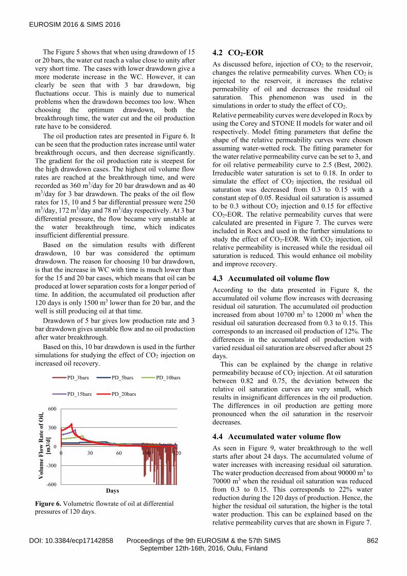
The oil production rates are presented in Figure 6. It

can be seen that the production rates increase until water

breakthrough occurs, and then decrease significantly.

The gradient for the oil production rate is steepest for

the high drawdown cases. The highest oil volume flow

rates are reached at the breakthrough time, and were

recorded as 360 m3/day for 20 bar drawdown and as 40

m3/day for 3 bar drawdown. The peaks of the oil flow

rates for 15, 10 and 5 bar differential pressure were 250

m3/day, 172 m3/day and 78 m3/day respectively. At 3 bar

differential pressure, the flow became very unstable at

the water breakthrough time, which indicates

insufficient differential pressure.

Based on the simulation results with different

drawdown, 10 bar was considered the optimum

drawdown. The reason for choosing 10 bar drawdown,

is that the increase in WC with time is much lower than

for the 15 and 20 bar cases, which means that oil can be

produced at lower separation costs for a longer period of

time. In addition, the accumulated oil production after

120 days is only 1500 m3 lower than for 20 bar, and the

well is still producing oil at that time.

Drawdown of 5 bar gives low production rate and 3

bar drawdown gives unstable flow and no oil production

after water breakthrough.

Based on this, 10 bar drawdown is used in the further

simulations for studying the effect of CO2 injection on

increased oil recovery.

Figure 6. Volumetric flowrate of oil at differential

pressures of 120 days.

4.2 CO2-EOR

As discussed before, injection of CO2 to the reservoir,

changes the relative permeability curves. When CO2 is

injected to the reservoir, it increases the relative

permeability of oil and decreases the residual oil

saturation. This phenomenon was used in the

simulations in order to study the effect of CO2.

Relative permeability curves were developed in Rocx by

using the Corey and STONE II models for water and oil

respectively. Model fitting parameters that define the

shape of the relative permeability curves were chosen

assuming water-wetted rock. The fitting parameter for

the water relative permeability curve can be set to 3, and

for oil relative permeability curve to 2.5 (Best, 2002).

Irreducible water saturation is set to 0.18. In order to

simulate the effect of CO2 injection, the residual oil

saturation was decreased from 0.3 to 0.15 with a

constant step of 0.05. Residual oil saturation is assumed

to be 0.3 without CO2 injection and 0.15 for effective

CO2-EOR. The relative permeability curves that were

calculated are presented in Figure 7. The curves were

included in Rocx and used in the further simulations to

study the effect of CO2-EOR. With CO2 injection, oil

relative permeability is increased while the residual oil

saturation is reduced. This would enhance oil mobility

and improve recovery.

4.3 Accumulated oil volume flow

According to the data presented in Figure 8, the

accumulated oil volume flow increases with decreasing

residual oil saturation. The accumulated oil production

increased from about 10700 m3 to 12000 m3 when the

residual oil saturation decreased from 0.3 to 0.15. This

corresponds to an increased oil production of 12%. The

differences in the accumulated oil production with

varied residual oil saturation are observed after about 25

days.

This can be explained by the change in relative

permeability because of CO2 injection. At oil saturation

between 0.82 and 0.75, the deviation between the

relative oil saturation curves are very small, which

results in insignificant differences in the oil production.

The differences in oil production are getting more

pronounced when the oil saturation in the reservoir

decreases.

4.4 Accumulated water volume flow

As seen in Figure 9, water breakthrough to the well

starts after about 24 days. The accumulated volume of

water increases with increasing residual oil saturation.

The water production decreased from about 90000 m3 to

70000 m3 when the residual oil saturation was reduced

from 0.3 to 0.15. This corresponds to 22% water

reduction during the 120 days of production. Hence, the

higher the residual oil saturation, the higher is the total

water production. This can be explained based on the

relative permeability curves that are shown in Figure 7.

-600

-300

0

300

600

0 30 60 90 120

Volu

me

Flo

w R

ate

of

Oil

,

[m3/d

]

Days


PD_15bars PD_20bars



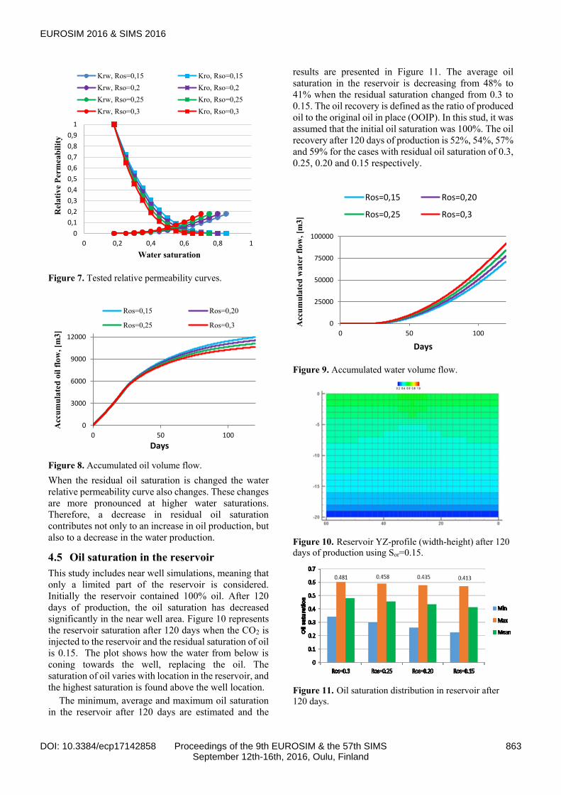
Figure 7. Tested relative permeability curves.

Figure 8. Accumulated oil volume flow.

When the residual oil saturation is changed the water

relative permeability curve also changes. These changes

are more pronounced at higher water saturations.

Therefore, a decrease in residual oil saturation

contributes not only to an increase in oil production, but

also to a decrease in the water production.

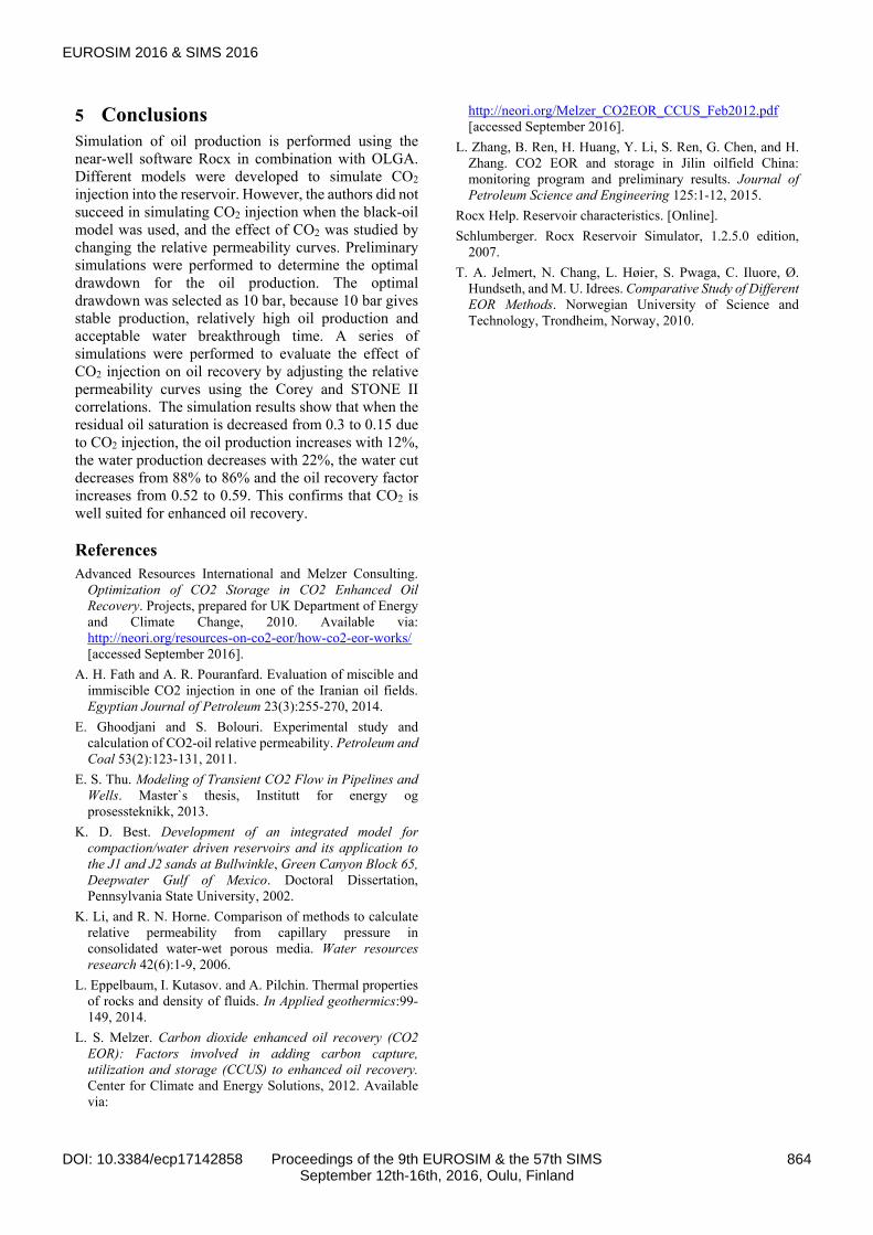
4.5 Oil saturation in the reservoir

This study includes near well simulations, meaning that

only a limited part of the reservoir is considered.

Initially the reservoir contained 100% oil. After 120

days of production, the oil saturation has decreased

significantly in the near well area. Figure 10 represents

the reservoir saturation after 120 days when the CO2 is

injected to the reservoir and the residual saturation of oil

is 0.15. The plot shows how the water from below is

coning towards the well, replacing the oil. The

saturation of oil varies with location in the reservoir, and

the highest saturation is found above the well location.

The minimum, average and maximum oil saturation

in the reservoir after 120 days are estimated and the

results are presented in Figure 11. The average oil

saturation in the reservoir is decreasing from 48% to

41% when the residual saturation changed from 0.3 to

0.15. The oil recovery is defined as the ratio of produced

oil to the original oil in place (OOIP). In this stud, it was

assumed that the initial oil saturation was 100%. The oil

recovery after 120 days of production is 52%, 54%, 57%

and 59% for the cases with residual oil saturation of 0.3,

0.25, 0.20 and 0.15 respectively.

Figure 9. Accumulated water volume flow.

Figure 10. Reservoir YZ-profile (width-height) after 120

days of production using Sor=0.15.

Figure 11. Oil saturation distribution in reservoir after

120 days.

0

3000

6000

9000

12000

0 50 100

Acc

um

ula

ted

oil

flo

w, [m

3]

Days

Ros=0,15 Ros=0,20

Ros=0,25 Ros=0,3 0

25000

50000

75000

100000

0 50 100

Acc

um

ula

ted

wate

r fl

ow

, [m

3]

Days

Ros=0,15 Ros=0,20

Ros=0,25 Ros=0,3

0

0,1

0,2

0,3

0,4

0,5

0,6

0,7

0,8

0,9

1

0 0,2 0,4 0,6 0,8 1

Rel

ati

ve P

erm

eab

ilit

y

Water saturation

Krw, Ros=0,15 Kro, Rso=0,15

Krw, Rso=0,2 Kro, Rso=0,2





5 Conclusions

Simulation of oil production is performed using the

near-well software Rocx in combination with OLGA.

Different models were developed to simulate CO2

injection into the reservoir. However, the authors did not

succeed in simulating CO2 injection when the black-oil

model was used, and the effect of CO2 was studied by

changing the relative permeability curves. Preliminary

simulations were performed to determine the optimal

drawdown for the oil production. The optimal

drawdown was selected as 10 bar, because 10 bar gives

stable production, relatively high oil production and

acceptable water breakthrough time. A series of

simulations were performed to evaluate the effect of

CO2 injection on oil recovery by adjusting the relative

permeability curves using the Corey and STONE II

correlations. The simulation results show that when the

residual oil saturation is decreased from 0.3 to 0.15 due

to CO2 injection, the oil production increases with 12%,

the water production decreases with 22%, the water cut

decreases from 88% to 86% and the oil recovery factor

increases from 0.52 to 0.59. This confirms that CO2 is

well suited for enhanced oil recovery.

References

Advanced Resources International and Melzer Consulting.

Optimization of CO2 Storage in CO2 Enhanced Oil

Recovery. Projects, prepared for UK Department of Energy

and Climate Change, 2010. Available via:

http://neori.org/resources-on-co2-eor/how-co2-eor-works/

[accessed September 2016].

A. H. Fath and A. R. Pouranfard. Evaluation of miscible and

immiscible CO2 injection in one of the Iranian oil fields.

Egyptian Journal of Petroleum 23(3):255-270, 2014.

E. Ghoodjani and S. Bolouri. Experimental study and

calculation of CO2-oil relative permeability. Petroleum and

Coal 53(2):123-131, 2011.

E. S. Thu. Modeling of Transient CO2 Flow in Pipelines and

Wells. Master`s thesis, Institutt for energy og

prosessteknikk, 2013.

K. D. Best. Development of an integrated model for

compaction/water driven reservoirs and its application to

the J1 and J2 sands at Bullwinkle, Green Canyon Block 65,

Deepwater Gulf of Mexico. Doctoral Dissertation,

Pennsylvania State University, 2002.

K. Li, and R. N. Horne. Comparison of methods to calculate

relative permeability from capillary pressure in

consolidated water‐wet porous media. Water resources

research 42(6):1-9, 2006.

L. Eppelbaum, I. Kutasov. and A. Pilchin. Thermal properties

of rocks and density of fluids. In Applied geothermics:99-

149, 2014.

L. S. Melzer. Carbon dioxide enhanced oil recovery (CO2

EOR): Factors involved in adding carbon capture,

utilization and storage (CCUS) to enhanced oil recovery.

Center for Climate and Energy Solutions, 2012. Available

via:

http://neori.org/Melzer_CO2EOR_CCUS_Feb2012.pdf

[accessed September 2016].

L. Zhang, B. Ren, H. Huang, Y. Li, S. Ren, G. Chen, and H.

Zhang. CO2 EOR and storage in Jilin oilfield China:

monitoring program and preliminary results. Journal of

Petroleum Science and Engineering 125:1-12, 2015.

Rocx Help. Reservoir characteristics. [Online].

Schlumberger. Rocx Reservoir Simulator, 1.2.5.0 edition,

2007.

T. A. Jelmert, N. Chang, L. Høier, S. Pwaga, C. Iluore, Ø.

Hundseth, and M. U. Idrees. Comparative Study of Different

EOR Methods. Norwegian University of Science and

Technology, Trondheim, Norway, 2010.



http://neori.org/resources-on-co2-eor/how-co2-eor-works/

http://neori.org/Melzer_CO2EOR_CCUS_Feb2012.pdf

Documents

Simulation of CO2 for Enhanced Oil Recovery2 Olga and Rocx or OLGA is a one-dimensional transient dynamic multiphase simulator used to simulate flow in pipelines and connected equipment