SIMULATION OF CO STORAGE IN SALINE AQUIFERSscience.uwaterloo.ca/~mauriced/earth691-duss/CO2_General CO2... · SIMULATION OF CO 2 STORAGE IN SALINE AQUIFERS ... Institute of Petroleum

SIMULATION OF CO2 STORAGE IN SALINE AQUIFERS

S. GHANBARI†, Y. AL-ZAABI‡, G. E. PICKUP, E. MACKAY�, F. GOZALPOUR and A. C. TODD

Institute of Petroleum Engineering, Heriot-Watt University, Edinburgh, UK

This paper evaluates key parameters in CO2 storage in saline aquifers. A reservoirsimulator was used to simulate 30 years of CO2 injection followed by 470 years ofshut in. Two retention mechanisms were modelled: hydrodynamic and solubility trap-

ping. Solubility trapping was found to be the most important means for storing CO2. Thiseffect was enhanced by the creation of convective flow patterns which lead to a greaterdissolution of CO2. Tests were carried out on a homogeneous model, and the effects ofCO2 diffusion in brine, vertical to horizontal permeability ratio, residual saturations, salinityand injection well completion interval were investigated. Results were compared with thosefrom other studies to develop a more general understanding of factors affecting CO2 storage.

To increase the realism of this study, the effect of geological heterogeneity was also exam-ined. Three types of heterogeneity were investigated: low level random variations in sand-stone permeability, stochastic shale layers and a fault. The low level heterogeneity did nothave a large effect, although it distorted the convective pattern, while the presence ofshales did have a large effect. CO2 tends to become trapped beneath the shale layers increas-ing the lateral migration. The amount of dissolved CO2 was largest in the models with anintermediate amount of shale. It was found that the fault did not affect the pressure distri-bution in the aquifer, unless the transmissibility was very low. However, the distribution ofCO2 was affected by the location of the well relative to the fault.

Keywords: CCS; CO2 storage; saline aquifers; geological heterogenity; resevoir simulation;convection; sensitivity studies.

INTRODUCTION

There has been a growing concern about the use of fossilfuels and its adverse effects on the atmosphere. With the‘business-as-usual’ projection of consumption of fossilfuels, the amount of CO2 in the atmosphere is likely torise dramatically, with serious consequences for the cli-mate. The growing concern in the global effects of green-house gases has resulted in several agreements betweengovernments. This is illustrated by international agreementssuch as the UN climate convention in Rio (1992), Kyoto(1997) and Buenos Aires (1998), committing the industrialcountries to reduce their emissions by approximately 5%compared with the 1990 level. This situation creates newtechnical and economic perspectives for the fossil fuelindustries.Under the current political and economic outlook it is

very unlikely that the dependency on fossil fuels (especiallyin developing countries with increasing populations) willdecrease. Therefore there is an urgent need to develop inno-vative strategies for CO2 stabilization to reduce emissionthrough improved energy efficiency and/or mitigate themthrough waste stream capture and storage. This approach

currently stands alone as a practical near-term means of sig-nificant storage of CO2 emissions.

Carbon dioxide abatement is a process by which carbondioxide is captured from large point sources and storedindefinitely. Geological storage is one the promisingoptions for storage of significant quantities of CO2 forlong-term time scales (Bentham and Kirby, 2005;Chadwick et al., 2001; Lindeberg and Bergmo, 2002).Carbon dioxide can be pumped into underground coal, oiland gas reservoirs and into saline aquifers. There isample evidence to suggest that these techniques canreliably retain stored carbon dioxide, as many naturallyformed carbon dioxide accumulations have been foundthroughout the world.

Deep saline aquifers seem to be the most promising sitesfor CO2 storage as they are widely distributed, underliemost point sources of CO2 emission and they are not lim-ited by the reservoir size, unlike depleted oil and gasreservoirs.

CO2 DISPOSAL IN SALINE AQUIFERS: PROCESSOVERVIEW

To avoid the problems with two phase flow within theinjection line and associated injection facilities CO2 isoften injected at supercritical conditions. The critical temp-erature and pressure for CO2 are 31.048C and 7.382 MParespectively. Therefore a minimum aquifer depth of

�Correspondence to: Dr E. Mackay, Herior-Watt University, Institute ofPetroleum Engineering, Riccarton, Edinburgh, EH14 4AS, UK.E-mail: [email protected]†Current address: National Iranian Oil Company, Iran.‡Current address: PDO, Oman.

764

0263–8762/06/$30.00+0.00# 2006 Institution of Chemical Engineers

www.icheme.org/cherd Trans IChemE, Part A, September 2006doi: 10.1205/cherd06007 Chemical Engineering Research and Design, 84(A9): 764–775

800 m is required to sustain supercritical pressure (Pruesset al., 2003). At conditions typical in the North Sea(pressure around 30 MPa and temperature of 808C) CO2

is supercritical with liquid-like properties and it is lessdense than the formation water (Pearce et al., 2000).The first and the only commercial scale project for CO2

disposal into the aquifer to-date is the Sleipner Vest project.It is operated by Statoil and is located in the Norwegiansector of the North Sea. The rich gas of the Sleipner Vestfield contains sizeable amounts of CO2 (9%), but the gassales contract limits the maximum amount of CO2 in theexported gas stream to 2.5%. CO2 is removed using an acti-vated amine and is injected into a large deep saline aquifer(Utsira formation) (Chadwick et al., 2002; Nghiem et al.,2004; Zweigel et al., 2001). This formation is locatedapproximately 800 m below the seabed. The CO2 injectionrate in this project is around 1 Mt per year since 1996 (Torpand Gale, 2003). Since then CO2 has been injected at thisrate without any significant operational problems.

CARBON DIOXIDE RETENTION MECHANISMS

A review of geological storage of CO2, including storagein brine aquifers, is presented by Orr (2004), and modellingstudies have been undertaken to simulate the process(Kumar et al., 2005; Lindeberg et al., 2001; Lindebergand Bergmo, 2002; Nghiem et al., 2004). Since CO2 isless dense than the brine, it will also rise, until it reachesa low permeability barrier (or cap rock). On the otherhand, CO2 is soluble in brine, and the resulting brine mix-ture is heavier than fresh brine, and so this mixture sinks. Aconvective process may occur, in which heavier brine withdissolved CO2 falls, and fresh brine rises (Ennis-King andPaterson, 2005). This process increases the amount ofCO2 dissolution, as it increases the contact area of freshbrine with CO2.There are several ways in which CO2 may be trapped.

Firstly, there is hydrodynamic trapping (e.g., Nghiem et al.,2004) where CO2, as a separate phase, is trapped beneathan impermeable cap rock. In addition, CO2 may be trappedat the pore-scale (Kumar et al., 2005). This mechanismoccurs in when the brine flows into a region previouslyinvaded by CO2 (which is an imbibition process). Theamount of trapping is influenced by the CO2-brine relativepermeability curves, including hysteresis and the residualCO2 saturation, which in turn depends on the rockcomposition and may vary from location to location.The second type of trapping is solubility trapping, men-

tioned above (e.g., Pruess et al., 2003). The phase beha-viour of the formation water–CO2 mixture controlsstorage in solution, and this depends on the water salinity,temperature and pressure. For example, the solubility ofCO2 in formation water at the prevailing temperature andpressure in the Utsira formation is reported to be approxi-mately 53 kg m23 (Torp and Gale, 2003).Thirdly, mineral trapping may occur. As CO2 dissolves

into the brine, the acidity increases leading to the dissol-ution of some rock minerals and the precipitation of sec-ondary minerals (e.g., Pruess et al., 2003; Kumar et al.,2005). Although mineral trapping is the most permanentretention mechanism, it takes place over longer timescales than considered in this study, so we do not considerit further in this paper.

NUMERICAL MODELLING APPROACH

Aquifer Model Description

In this study CO2 storage in a saline aquifer is modelled,using a reactive transport reservoir simulator (ComputerModelling Group, 2005). It is assumed that dissolutionoccurs instantaneously, therefore the CO2 gas rich phase isalways in equilibrium with the water phase with which it isin contact. We also assumed isothermal conditions of 378C.In the first part of this work, we have used a homogeneousmodel to study the effects of the following parameters onCO2 storage: CO2 diffusion in brine, vertical to horizontalpermeability ratio (kv/kh), residual gas and water saturation,salinity and injection well completion interval. Additionaltests on a heterogeneous model are described later.

The dimensions of the aquifer model were 8 km � 8 kmwith a thickness of 200 m. The horizontal permeability (kh)was 4000 md, the vertical permeability (kv) was 400 mdand the porosity was 37%. The model was specified to beinitially in static equilibration, with an initial aquiferpressure of 6.205 MPa at a depth of 620 m. The initialwater saturation was 100% and the salinity of the formationwater is assumed to be 3.2% by weight. There was nodissolved gas in the aqueous phase at the beginning ofthe simulation. The aquifer model was uniformly griddedin the three principal directions with 35 cells in x- andy-directions and 25 cells in the z-direction. The modeldetails are summarized in Table 1.

One injectorwas placed in the centre of the aquifermodel atblock (18,18). Pure CO2 was injected for 30 years into layer10, and this was followed by a 470 year shut-in periodwhere density differences provide the driving force. The injec-tion ratewas set to 1.46 � 104 m3 day21) (approx. 10 kt y21).

All calculations presented here are based on solubilitydata by Torp and Gale (2003). In fact, data that is more

Table 1. Details of the homogeneous model.

Grid 35 � 35 � 25Length 8 kmWidth 8 kmThickness 200 mDip angle 08Horizontal permeability 4000 mDVertical permeability 400 mDPorosity 37%Depth of top structure 620 mInitial pressure

(at datum 620 m)6.205 MPa

Initial temperature 378CInitial water saturation 100%Residual water saturation 0.105Water end point relative

permeability0.595

Residual gas saturation 0.05Gas end point relative

permeability1.0

Brine salinity 3.2% by weightInjection rate 1.46 � 104 m3 day21

(0.514 MMscf/d)Injection point cell (18, 18, 10)Components H2O CO2

Molecular weight 18.0 g gmole21 44.0 g gmole21

Mass density at6.205 MPa and 378C

1.019 � 103 kg m23 1.256 � 103 kg m23

Critical pressure 22.05 MPa 7.38 MPaCritical temperature 374.158C 31.18C

Trans IChemE, Part A, Chemical Engineering Research and Design, 2006, 84(A9): 764–775

SIMULATION OF CO2 STORAGE IN SALINE AQUIFERS 765

representative over wider temperature and pressure rangesis available in the literature (e.g., Duan and Sun, 2003),although in this case the emphasis of this work is on devel-oping a qualitative rather than quantitative understanding ofthe process. The viscosity of water with dissolved CO2 wascalculated through an internal algorithm within the soft-ware, and an allowance was made for the correction ofwater viscosity due to the effect of salinity. In this studythe effect of capillary pressure was ignored.

Relative Permeability Data

Among different proposed relative permeability curvesfor CO2–water–rock systems, the following sets of relativepermeability models, which have been developed for atypical sand system, were used (Pruess et al., 2003):

krl ¼ffiffiffiffiffiS�

p1� (1� ½S��1=m)m� �2

krg ¼ (1�

�

S)2(1�

�

S2)

where

S� ¼ (Sl � Slr)=(1� Slr)

�

S ¼ (Sl � Slr)=(1� Slr � Sgr)

Sl is the irreducible water saturation, which was set to0.105. The residual CO2 saturation, Sgr was 0.05, and theparameter m was equal to 0.6269. In this study, we usedthe same relative permeability curves to model CO2 displa-cing water and water displacing CO2 (no hysteresis in rela-tive permeability). Figure 1 shows the relative permeabilitycurves.

Simulation Results for Homogeneous Model

For the homogeneous model, offtake at the outer bound-ary of the model was simulated by means of productionwells. These wells maintain reservoir pressure constant,effectively removing brine at the same (downhole) rate as

gas is injected. Gas does not reach the outer boundary ofthe model within the time frame of the simulations—thusall injected gas is conserved within the system. The resultsare presented as a series of figures which show thedistribution of the following quantities: the gas saturation,the CO2 mole fraction in the aqueous phase, the aqueousphase density, the pH value. Figures 2, 3 and 4 illustratethe profiles at the time of shut-in, 100 years after shut-inand at the end of the simulation (500 years). In allof these figures, the model was cut-off in the J-directionat J ¼ 18, the plane containing the injector, so that thedistribution of the various quantities can be clearly seen.

Free Gas Profile [Figures 2(a), 3(a) and 4(a)]

During the injection period, the gas plume rises andimmiscible CO2 reaches the top of the model within thefirst year. Once at the top of the model, the CO2 migrateslaterally. After shut-in, the free gas in the plume movesup and the residual gas dissolves. At 22 years after shutin, all the free gas is in the top layer.

Dissolved CO2 [Figures 2(b), 3(b) and 4(b)]

The dissolution of CO2 into the saline water leads to anincrease in the density of the mixture in the order of 2–3%compared with fresh brine. Therefore the CO2 saturatedaqueous phase sinks, and as it does so, fresh formationwater rises and comes into contact with the gas cap. Thispromotes the process of dissolution. Note that this is a con-vective process similar to convective heat transfer (Ennis-King and Paterson, 2005).

There is significant solubility trapping within the gasplume. The residual water saturation within thegas plume is in equilibrium with the gaseous phase andthe mole fraction of the CO2 in the residual water ishigher than elsewhere in the aquifer, since the gas andresidual water are in direct contact.

The structure of the top of the aquifer may have a signifi-cant influence on the results. If the aquifer has a structuraltrap like a dome, then the gas may concentrate in this small

Figure 1. The relative permeability curves.


766 GHANBARI et al.

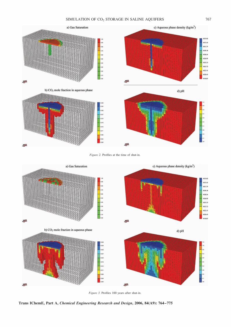
Figure 2. Profiles at the time of shut-in.

Figure 3. Profiles 100 years after shut-in.



region, and this will tend to reduce the amount of CO2

dissolution. However, if the top of the aquifer is extendedlaterally, more gas will migrate laterally, leading to anincrease in the aerial contact between the gas and water,so more CO2 may dissolve. But, in this case, there maybe a danger of gas leakage through the lateral boundariesof the aquifer.

Fine-Scale Distribution and Flow Patterns

It is interesting to examine the distribution of free anddissolved gas in more detail. Figure 5 shows a plot of thegas saturation in the top layer after 500 years, as a functionof distance from a point directly above the injection well. Itcan be seen that the saturation fluctuates. This distributionis similar along any radius moving outwards from cell(18,18,1), so the gas saturation in the top layer is in theform of rings (Figure 6). This pattern of rings may beunderstood by studying the flows of gas and water. Wehave examined the flows in the top layer of the modeland in the vertical plane at J ¼ 18, and summarize thesein a schematic diagram in Figure 7.The movement of water is best described in terms of a 2D

vertical cross section. Note that in 2D, the gas forms a ‘T’shape. After shut-in the gas starts to dissolve into thebrine, making it heavier so that it slumps. As it slumps, itmixes with fresh brine which dilutes it. The dilutiondecreases the velocity of the slumping (due to a decreasein density) and therefore the rate of CO2 dissolutiondecreases. This makes the horizontal bar of the T-shape

relatively stable. However, at the borders of this region,the gas is in contact with more brine, and the brine migrateslaterally inwards. At the edge of the T-shape there is there-fore more dissolution of CO2 in brine and more slumping.This is why the T-shape droops at the sides.

Also there is a large amount of water slumping in thecentre of the model (the vertical part of the T-shape andbelow it). As CO2 is injected, it rises, and partly dissolvesin the brine, which becomes heavier and then slumps. Thisshows that there are two main regions where slumpingoccurs: one in the centre of the model, and the other atthe edge of the T-shape. However, there is also a smallamount of slumping halfway between the centre and

Figure 4. Profiles after 500 years.

Figure 5. Gas saturation profile at the top layer at the end of simulation(after 500 years).


768 GHANBARI et al.

the edge of the T-shape (Figure 7). This suggests that con-vection is developing in a manner predicted by Ennis-Kingand Paterson (2005). [In fact, as noted by Ennis-King andPaterson (2005), a finer grid may resolve more fingersof descending CO2-rich brine.] In plain view from thetop, this convection gives rise to rings of high and lowgas saturations, as shown in Figure 6.In the base case calculation, 55.8% of the total injected

CO2 was dissolved in the water phase after 500 years. Ofthe fraction of CO2 remaining in the gas phase, some istrapped as residual gas, and some is free gas that hasmigrated to the top of the structure.A series of sensitivity studies was performed to

determine the effect of the diffusion coefficient, the kv/khratio, the residual gas and water saturations, salinity and the

location of the injection well completion. The values of theparameters used in these tests are shown in Table 2.

Effect of CO2 Diffusion in Water

The dissolution of CO2 into the brine induces CO2 con-centration gradients, which in turn causes CO2 to diffusewithin the aquifer. The results indicate that after 500years more gas has been immobilized in the form ofsolubility trapping. Due to the diffusion process the CO2

concentration in each grid block is higher than CO2 concen-tration in the base case model. The diffusion promotes thetransportation of CO2 in any grid block leading to dissol-ution of more CO2 and consequently enhances the effec-tiveness of solubility trapping.

Figure 6. Aerial view of gas saturation profile after 500 years. The legend shows the gas saturation, and the concentric rings indicate the maxima and minimain the gas saturation distribution.

Table 2. Values of parameters used in the sensitivity study and impact ondissolved CO2 in water after 500 years.

Sensitivity calculations CO2 dissolved in waterafter 500 years

CO2 diffusionWithout diffusion (base case) 55.8%With diffusionDiffusion coefficient for CO2 at 378C2.6 � 1029 m2 s21

79.1%

kv/kh ratiokv/kh ¼ 0.1 (base case) 55.8%kv/kh ¼ 1.0 76.5%kv/kh ¼ 0.01 37.4%

Residual water (Swr) and gas (Sgr) saturationsSwr ¼ 0.105; Sgr ¼ 0.05 (base case) 55.8%Swr ¼ 0.3; Sgr ¼ 0.3 52.4%

Salinity3.2% by weight (base case) 55.8%10.0% by weight 39.2%

Injection pointCell (18,18,10) (base case) 55.8%Cell (18,18,1) 45.1%

Figure 7. Schematic diagram of flows of brine after 100 years shut in. Thethickness of the arrows indicates the flux. Dark blue arrows show thedescent of brine and dissolved CO2, light blue arrows indicate the scentof fresh brine. The small black circle in the centre shows the location ofthe injector. The coloured squares at the top of the model indicate thegas saturation, with red representing a high gas saturation. (Note thatonly part of the model is shown for clarity.)



Effect of kv/kh Ratio

An increase in the kv/kh ratio increases the amount ofcarbon dioxide which is immobilized due to solubility trap-ping. As this ratio increases the rate of vertical migration ofgas during injection period increases. After shut-in, thewater–CO2 mixture starts to slump, and the rate of slump-ing will be greater the higher kv/kh, leading to yet moredissolution. Therefore the amount of dissolution is muchhigher in the high kv/kh case. As the kv/kh ratio decreases,the lateral migration will become dominant and ultimatelythere might be a concern about possible gas leakagethrough the aquifer boundaries.

Effect of Residual Gas and Water Saturations

The effect of increasing the residual water saturation isbeneficial in terms of ultimate storage capacity of the aqui-fer. As the gas is being injected it displaces the waterthrough immiscible displacement in the top layer andoccupies its place. However, a residual amount of watersaturation remains. This water is in direct contact withgas and is in equilibrium with gas at that pressure andtemperature. The concentration of carbon dioxide in theresidual water in this region is the highest throughout theaquifer. Therefore an increase in the residual watersaturation is beneficial in terms of dissolving largerquantities of gas within the gas plume.The effect of increasing the residual gas saturation is to

immobilize larger quantities of gas within the gas plume.It is in fact beneficial because while at the same time itdecreases the effectiveness of solubility trapping mechan-isms, it offers a promising alternative to immobilize largequantities of gas in the form of residual gas saturation.In the cases studied here, we increased both Swr and Sgr,

and the overall result was a slight decrease in the amount ofCO2 dissolved.

Effect of Salinity

As the salinity increases two effects contribute to reducethe effectiveness of solubility trapping. The first effect isthe reduction in solubility of CO2 in formation water.The second effect is the increase in the partial molarvolume of water. As the salinity increases, the differencebetween partial molar volume of water and CO2 decreases.Therefore the effectiveness of convective flow mixingdecreases significantly. Therefore, the increase in salinitysignificantly decreases the solubility.

Effect of Injection Well Completion Interval

When the well was completed in layer 10, the gas satur-ation around the injection well was still very high, around0.9 after 500 years. However when the well was completedin the top layer, contrary to expectations, the simulationshowed that the gas saturation was much lower, around0.1. Also, comparison between this model and the basecase model shows that, after 500 years, less CO2 is trappedin the form of solubility trapping when the well is com-pleted in the top layer. These results can be explainedusing Figure 8, which illustrates the direction of waterflow within the aquifer when the well is completed in toplayer. Completing the well in the top layer causes the

injected gas to spread away from the injector almost instan-taneously and therefore there is no water slumping at thecentre of the plume. However, in this case water slumpingat the borders of the gas plume is dominant. After slumpingto the base of the model, water starts to return upward fromthe centre of the gas cap and simultaneously sweeps the gasoutward and at the same time dissolves it. As illustrated inFigure 9, after 500 years gas is swept outward from theinjection zone in the top layer completion model. In thissituation the solubility trapping has been decreased. How-ever at the same time gas has been pushed away from theinjection zone. This is very beneficial in terms of the qual-ity of the cement job. If after, for instance, 500 years thereis some leakage due to the failure of the cement, the gassaturation around the injection zone has been decreasedconsiderably and there is less danger compared to whenthe gas saturation around the injection well is about 0.9.

COMPARISON WITH OTHER RESULTS

The simulation of CO2 injection into saline aquifers hasbeen performed by a number of different research groups(e.g., Pruess et al., 2003; Nghiem et al., 2004; Kumaret al., 2005; Hovorka et al., 2004). While there is broadagreement between authors, there are some differences,and it is worth comparing the results. For example, thesimulations by Nghiem et al. (2004) and Ennis-King andPaterson (2005) show evidence of convection due to thebrine with dissolved CO2 being denser than pure brine.However, Pruess et al. (2003) and Kumar et al. (2005) donot show this effect. In the case of Pruess et al. (2003),this is because they do not model any change in the densityof brine with dissolved CO2. Since Hovorka et al. (2004)(mentioned below) use the same fluid properties as Pruesset al. (2003), they do not demonstrate any convectioneither. On the other hand, Kumar et al. (2005) do takeaccount of the increase in the density of brine with dissol-ution of CO2. They point out that this increase in densitydecreases with increasing salinity. However, in their basecase model, the density difference is about 1%, which isthe same as the value used by Ennis-King and Paterson

Figure 8. Schematic diagram of the flow of brine in the case where thewell is in the top layer. The thickness of the arrows indicates the flux.Dark blue arrows show the descent of brine and dissolved CO2, lightblue arrows indicate the scent of fresh brine. The small black circle inthe centre shows the location of the injector. The coloured squares at thetop of the model indicate the gas saturation, with red representing a highgas saturation. (Note that only part of the model is shown for clarity.)


770 GHANBARI et al.

(2005) for studying convection. It may be that, in the caseof Kumar et al. (2005), their low value of kv/kh (for thebase case) has suppressed convection, or that the highlevel of heterogeneity in some of their models has dispersedthe descending fingers of high density brine.Note that while Pruess et al. (2003) conclude that the

effectiveness for CO2 storage decreases with increasingkv/kh, Ennis-King and Paterson (2005) conclude that a highkv/kh ratio is more beneficial, because this encouragesconvective mixing.

THE EFFECT OF HETEROGENEITY

Rocks are naturally heterogeneous, and this has to betaken into account when modelling CO2 storage. Differenttypes of heterogeneities arise in different depositionalenvironments. In this study we focus on rocks similar tothose in the Utsira Formation, which is the formationused for CO2 injection near the Sleipner Field. An introduc-tion to the geology of this formation is given by Zweigelet al. (2004). Although there is some dispute as the todepositional environment of the Utsira formation, it isusually assumed that the Utsira sandstone was depositedas massflows or turbidite sands. The sandstone is unconso-lidated and has a high porosity and permeability, with akv/kh ratio of approximately 1. However, several thinshale layers (�1 m thick) have been detected in seismicand wireline measurements. These are expected to havevery low permeability, so that they act as baffles or partialbaffles. They are not expected to be continuous, though, sothat CO2 can migrate around them.Additional studies on the effect of geological heterogeneity

have been carried out by Hovorka et al. (2004), using the Friosandstone in Texas as an example. Some of the models theyconsidered include shale layers, and they point out that hetero-geneity can aid the storage of CO2, by dispersing the flowpaths, bringing the CO2 into contact with more brine.In the present work, three types of heterogeneity were

investigated, the first two being related to the Utsira for-mation. Firstly, we examined the effect of low levelrandom variations in the permeability of the high per-meability sandstone, and secondly we added stochasticshales to the model. In the third case, we investigated the

effect of a fault, although no large-scale faulting has beendetected in the Utsira formation. In all the models used forthe heterogeneity study the grid size was 32 � 32 � 24,and the horizontal dimensions for each cell were243.8 m � 243.8 m. In the models for the random heteroge-neities and the fault, the cells were of uniform thickness of6.55 m. In the shale models, the total thickness of themodel was the same, but the thickness was 7.62 m for thesandstone layers and 1.22 m for the shale layers.

Effect of Random Permeability Variations

Stochastic permeability and porosity models were cre-ated using sequential Gaussian simulation (Journel andHuijbrechts, 1978). Several models were generated, asshown in Table 3. In each case the average permeabilitywas 4000 mD and the porosity, f, was calculated byassuming that it was proportional to log permeability, k,using the following equation:

f ¼ 0:01þ 0:1 � log10 (k) (10)

An example of one of the models is shown in Figure 10.The results for one of these models are shown in

Figure 11. (The results for the other models were broadlysimilar.) They indicate that this level of heterogeneitydoes not have a large effect on the distribution of freeCO2 gas, or dissolved CO2. The gas plume still risesto the top of the model [Figure 11(a)]. However, theT-shape is distorted, as one might expect [Figure 11(b)],because flow through the model will be concentrated onhigh permeability flow paths. Also the ring pattern in thegas saturation in the top layer is distorted [Figure 11(c)].

Table 3. The standard deviations and correlation lengths used in thestochastic sandstone models.

Modelnumber

Standarddeviation (mD)

Correlation lengths (m)

Horizontal Vertical

1 1000 1951 26.22 1000 975 13.13 300 1951 26.24 300 975 13.1

Figure 9. Gas saturation in top layer after 500 years. [Well completed in layer 10 shown on left (base case model) and well completed in top layer on right.]



Although the standard deviations in these models appearto be large (1000 mD and 300 mD), these models are not, infact high heterogeneity models. The coefficient of variation,Cv, is defined as standard deviation/average. In the modelshere, Cv in permeability is 0.25 and 0.075, whereas in veryheterogeneous models, it may be greater than 1. However,this level of heterogeneity is quite typical of massive highpermeability sandstones, such as the Utsira sandstone.

Effect of Shale Layers

Reservoirs frequently contain shale layers, and it isknown from studies of the Utsira aquifer that there areshale layers present (e.g., Zweigel et al., 2004). For thisstudy, a set of models were generated with four horizontalshaley layers (Al-Saaidi, 2004), using the method devel-oped by Stephen et al. (2001). All the models had thesame dimensions as the previous model. In each model, adifferent percentage of shale was specified for the layers:

Model 1: 90% shale in each ‘shale’ layer,Model 2: 50% shale in each ‘shale’ layer,Model 3: 25% shale in each ‘shale’ layer.

Each shale layer was 1.22 m thick and the cells with shalewere assigned zero porosity and zero permeability. Theremainder of each model consisted of high permeabilitysandstone of 4000 mD, with kv/kh ¼ 1. In all cases, CO2

was injected into the centre of the bottom layer.In general, the shale layers prevent the gas moving up

vertically, and also prevent the water saturated with CO2

moving vertically down, so there is therefore more lateralmovement. The degree to which this occurs depends onthe percentage of shale, as discussed below.

The results for the 90% shale case are shown inFigure 12. It can be seen that the shale has prevented theCO2 gas from reaching the top of the model[Figure 12(a)], and the saturation is highest in two ‘gascaps’ beneath shales in the first and second shaley layers.It can be seen that CO2 saturated brine is distributedbeneath the CO2 gas caps. There are no T-shapes in thiscase, but this may be because the model is not fineenough to resolve them.

When the percentage of shale is reduced to 50%, thereare more gaps in the shales and so the CO2 gas can migratefurther, although it does not reach the top of the model[Figure 13(a)]. The CO2 saturated brine is distributedfairly uniformly in the regions invaded by the gas[Figure 13(b)].

Figure 14 shows the results for the 25% shale model. Inthis case there are sufficient gaps in the shales for the gas toreach the top of the model by the time of shut-in[Figure 12(a)]. The CO2 saturated brine is distributedfairly uniformly in a block which extends from the top tothe bottom of the model [Figure 14(b)].

Note that we have only shown the results for one realis-ation of each model here. Different realisations will havegaps in the shales in different places, so the distributionsof free and dissolved CO2 will vary. However, the overallpicture is clear: an impermeable shale body will stop thevertical rise of the CO2 gas, and will encourage lateralmovement of the gas beneath the shale. This lateral move-ment will continue until a gap in the shale is encountered(unless the lateral movement has stopped because the

Figure 10. Example of one of the models with random heterogeneities (toplayer only). This model had a short correlation length and high standarddeviation.

Figure 11. The simulation results for themodel in Figure 10, after 289 years.


772 GHANBARI et al.

injection has ceased, or the CO2 has all dissolved in thebrine). The higher the percentage shale the more likelythe gas will become trapped beneath one of the lowershales. The effect of the shales on the distribution of dis-solved CO2 is to inhibit the downward movement of theheavier brine, and again encourage more lateral movement.The characteristic T-shape which develops in the homo-geneous model is no longer present, and the CO2 saturatedbrine seems to have a more uniform distribution in theregions invaded by the CO2 gas. However, this may bepartly due to lack of resolution in the model.

Effect of a Fault

In the third heterogeneous model, a fault was placedin the plane I ¼ 14. It had a throw of 6.55 m, and was1 cell thick in the I-direction, and extended across thewhole model in the J- and K-directions. The cells on theleft of the model were shifted down relative to the cellson the right. The transmissibility of the fault was variedfrom 0 (complete barrier) to 1 (no effect). The well wasinitially placed at location I ¼ 16, J ¼ 16 and completedin layer K ¼ 10.Figure 15 shows the pressure in the well block as a func-

tion of time for different fault transmissibilities. Asexpected the greatest increase in pressure occurs whenthe fault transmissibility is zero—i.e., the fault is comple-tely sealing. When injection stops after 30 years, the

Figure 13. The results for the 50% shale model. Top: the free gas satur-ation at the time of shut-in. Bottom: the CO2 mole fraction in the aqueousphase, 100 years after shut-in.Figure 12. The results for the 90% shale model. Top: the free gas satur-

ation at the time of shut-in. Bottom: the CO2 mole fraction in the aqueousphase, 100 years after shut-in.

Figure 14. The results for the 25% shale model. Top: the free gas satur-ation at the time of shut-in. Bottom: the CO2 mole fraction in the aqueousphase, 100 years after shut-in.



pressure decreases due to the dissolution of CO2 in brine.The largest decrease occurs in the case of the sealing fault.When the transmissibility is non-zero, one would expect

that the CO2 gas would flow across the fault. However, asshown in Figure 16, the well is in the upper of the two com-partments, so the gas stays in this compartment because ofbuoyancy. It is only when the well is moved to the left(lower) side of the fault that the gas plume forms on bothsides of the fault (Figure 17).The distribution of dissolved CO2 therefore depends cri-

tically on the location of the well. If the well is on the rightside of the fault (upper compartment), the dissolved CO2

forms largely in that compartment, even when the transmis-sibility is high. On the other hand, when the well is on theleft side of the fault (lower compartment), the dissolvedCO2 is distributed on both sides of the fault, because thegas plume is on both sides.

CONCLUSIONS

In this paper CO2 storage in a deep saline aquifer hasbeen presented, with emphasis on the hydrodynamic andsolubility trapping mechanisms. The convective flow-mixing pattern within the homogeneous aquifer due to theincrease in the CO2-brine density has been shown to playthe most important role in the ultimate fate of CO2 as itpromotes further dissolution of carbon dioxide.

The effect of CO2 diffusion rate in brine was found to bevery important with respect to the ultimate distribution ofCO2 between various phases. Also the kv/kh ratio had a signifi-cant effect: at low kv/kh ratios where there is more lateralmigration of the gas and the efficiency of vertical slumpingprocess decreases significantly, while an increase in thisratio is beneficial as it enhances the convective flow patternwithin the aquifer leading to more CO2 trapped in the formof dissolution trapping. Salinity was found to decrease theeffectiveness of solubility trapping drastically and leaves ahigh percentage of CO2 in the gas phase. Increase in theresidual gas saturation was found to be very beneficial interms of immobilizing large quantities of CO2 while at the

Figure 15. The pressure in the well block as a function of time for differentfault transmissibilities.

Figure 16. The results for the well in the upper block. The fault transmis-sibility was 0.5. Top: the free gas saturation at shut-in. Bottom: the molefraction of CO2 in the aqueous phase, 100 years after shut-in.

Figure 17. The results for the well in the lower block. The fault transmis-sibility was 0.5. Top: the free gas saturation at shut-in. Bottom: the molefraction of CO2 in the aqueous phase, 290 years after shut-in.


774 GHANBARI et al.

same time decreasing the solubility of CO2 in brine. Increasein residual water saturation is in fact beneficial as it allowsmore of the CO2 in the gas plume to dissolve. The effect ofcompleting the well in the middle or bottom layers givesbenefit in terms of increasing the solubility of CO2 in brine;however it leaves high gas saturation even after 500 yearsaround the injection well.

CONCLUSIONS FROM HETEROGENEITY STUDY

The low level heterogeneity did not have much effect,although it did distort the pattern in the gas saturationwhich was seen in the homogeneous case.The presence of shales did, however, have a large effect. As

the percentage of shale increases, theCO2 gas tends to becometrapped beneath the lower layers of shale and moves laterallyrather than vertically. The amount of dissolved CO2 tends tobe larger in the models with an intermediate amount of shale.A fault does not affect the pressure distribution in the

aquifer, unless the transmissibility is very low (tending tozero). However the distribution of the free and dissolvedCO2 was affected by the location of the well, even whenthe transmissibility was 1, when it might be expected tohave no effect. If the well was placed in the upper compart-ment, the gas only rose upwards in this compartment, anddissolved CO2 stayed mainly in this compartment.

IMPLICATIONS FOR GEOLOGICAL STORAGEOF CO2 IN HETEROGENEOUS AQUIFERS

The first part of this paper compared the importance ofdifferent mechanisms for CO2 trapping as a function ofvarious parameters. It was shown that the most importanttrapping mechanism at time scales of a few 100 years issolubility trapping, depending on the assumptions madeabout diffusion and the impact of reservoir properties,such as kv/kh, residual saturation, formation brine salinityand the location of the injection point, although hydro-dynamic trapping is also significant under all the scenariosstudied. The dissolution of CO2 is enhanced by the fact thatconvective movement is set up in the aquifer with freshbrine moving upwards and CO2-saturated brine movingdownwards. Therefore the best type of aquifer for storingCO2 is one where solubility trapping is maximized.

NOMENCLATURE

k absolute permeability (mD) [L2]kv absolute permeability in the vertical direction (mD) [L2]kh absolute permeability in the horizontal direction (mD) [L2]kr relative permeability (dimesionless)S saturation (dimensionless)Swr irreducible water saturation (dimensionless)Sgr residual gas saturation (dimensionless)f porosity (dimensionless)

REFERENCES

Al-Saaidi, F., 2004, Co2 storage in heterogeneous rocks, MSc thesis,Heriot-Watt University.

Bentham, M. and Kirby, G., 2005, CO2 Storage in Saline Aquifers, Oil &Gas Science and Technology—Revue de l’Institut Francais du Petrole,60(3): 559–567.

Chadwick, A., Kirby, G., Holloway, S., Zweigel, P. and Arts, R., 2001,The case for underground carbon dioxide sequestration in Northern

Europe, European Union of Geosciences, 2001 meeting, Strasbourg(FR), abstract volume 172.

Chadwick, R.A., Zweigel, P., Gregersen, U., Kirby, G.A., Holloway, S.and Johannessen, P.N., 2002, Geological characterisation of CO2

Storage sites: Lessons from Sleipner, Northern North Sea, GHGT-6Proceedings, October 2002, Kyoto.

Computer Modelling Group, 2005, STARS User’s Guide.Duan, Z. and Sun, R., 2003, An improved model calculating CO2 solubility

in pure water and aqueous NaCl solutions from 273 to 533 K and from 0to 2000 bar, Chemical Geology, 193: 257–271.

Ennis-King, J. and Paterson, L., 2005, Role of convective mixing in thelong-term storage of carbon dioxide in deep saline formations, SPEJournal, 10(3): 349–356.

Hovorka, S.D., Doughty, C., Benson, S.M., Pruess, K. and Knox, P.R.,2004, The impact of geological heterogeneity on CO2 storage in brineformations: A case study form the Texas Gulf Coast, in Baines, S.J.and Worden, R.H. (eds). Geological Storage of Carbon Dioxide,Specials Publications, 233: 147–163. (Geological Society, London).

Journel, A.G. and Huijbrechts, C.J., 1978,Mining Geostatistics (AcademicPress, London, UK).

Kumar, A., Ozah, R., Noh, M., Pope, G.A., Bryant, S., Sephehrnoori, K.and Lake, L.W., 2005, Reservoir simulation of CO2 storage in deepsaline aquifers, SPE Journal, 10(3): 336–348.

Lindeberg, E. and Bergmo, P., 2002, The long-term fate of CO2 injectedinto an aquifer, in Proceeding of the 6th International GreenhouseGas Control Technologies, Kyoto, October 2002.

Lindeberg, E., Zweigel, P., Bergmo, P., Ghaderi, A. and Lothe, A., 2001,A prediction of CO2 dispersal pattern improved by geology and reser-voir simulation and verified by time lapse seismic, in: Williams, D.,Duri, B., McMullan, P. and Paulson, C. (eds). Greenhouse Gas ControlTechnologies 5, (CSIRO Publishing, Australia).

Nghiem, L., Sammon, P., Grabenstetter, J. and Ohkuma, H., 2004,Modeling CO2 storage in aquifers with a fully coupled geochemicalEOS compositional simulator, SPE 89474, presented at the SPE/DOEConference on Improved Oil Recovery, Tulsa, Oklahoma, 17–21April 2004.

Orr, F.M. Jr, 2004, Storage of carbon dioxide in geologic formations, J PetTech, (Sept. 2004): 90–97.

Pearce, J.M., Czernichowski-Lauriol, I., Rochelle, C.A., Springer, N.,Brosse, E., Sanjuan, B., Bateman, K. and Lanini, S., 2000, How willreservoir and caprock react with injected CO2 at Sleipner? Preliminaryevidence from experimental investigations, 5th International Confer-ence on Greenhouse Gas Control Technologies, Cairns (Australia),August 2000.

Pruess, K., Xu, T., Apps, J. and Garcia, J., 2003, Numerical modeling ofaquifer disposal of CO2, SPE Journal, 8(1): 49–60.

Stephen, K.D., Clark, J.D. and Gardiner, A.R., 2001, Outcrop based sto-chastic modelling of turbidite amalgamations and its effects on hydro-carbon recovery, Petroleum Geoscience, 7: 163–172.

Torp, T.A. and Gale, J., 2003, Demonstrating storage of CO2 in geologicalreservoirs: The Sleipner and SACS projects, in Vol. 1, J. Gale, J. andKaya, Y. (eds). Greenhouse Gas Control Technologies, 311–316(Elsevier, Amsterdam).

Zweigel, P., Arts, R., Bidstrup, T., Chadwick, A., Eiken, O., Gregersen, U.,Hamborg,M., Johanessen, P., Kirby, G., Kristensen, L. and Lindeberg, E.,2001, Results and experiences from the first industrial scale under-ground CO2 sequestration case (Sleipner field, North Sea), AmericanAssociation of Petroleum Geologists Annual Meeting, Denver (CO),abstract volume (CD).

Zweigel, P., Arts, R., Lothe, A.E. and Lindberg, E.B.G., 2004, Reservoirgeology of the Utsira formation at the first industrial-scale undergroundCO2 storage site (Sleipner area, North Sea), in Baines, S.J. andWorden, R.H. (eds). Geological Storage of Carbon Dioxide, SpecialsPublications, 233: 165–180 (Geological Society, London).

ACKNOWLEDGEMENTS

The authors would like to thank Karl Stephen for providing the softwarefor generating the stochastic shale model, and Faisal Al-Saaidi for creatingthese models. Computer Modelling Group are thanked for use of theSTARS simulation software in these calculations. Scottish FundingCouncil are thanked for financial support for the Scottish Centre forCarbon Storage Research Projects.

The manuscript was received 13 January 2006 and accepted forpublication after revision 23 May 2006.



Documents

SIMULATION OF CO STORAGE IN SALINE AQUIFERSscience.uwaterloo.ca/~mauriced/earth691-duss/CO2_General CO2... · SIMULATION OF CO 2 STORAGE IN SALINE AQUIFERS ... Institute of Petroleum