Embed Size (px)
Citation preview

SIMULATION OF A FLEXIBLE MANUFACTURING SYSTEM: A PILOT IMPLEMENTATION
A THESIS SUBMITTED TO THE GRADUATE SCHOOL OF NATURAL AND APPLIED SCIENCES
OF MIDDLE EAST TECHNICAL UNIVERSITY
BY
NECATİ DENİZ YÜCEL
IN PARTIAL FULFILLMENT OF THE REQUIREMENTS FOR
THE DEGREE OF MASTER OF SCIENCE IN
MECHANICAL ENGINEERING
SEPTEMBER 2005

Approval of the Graduate School of Natural and Applied Sciences
Prof. Dr. Canan ÖZGEN
Director
I certify that this thesis satisfies all the requirements as a thesis for the degree of Master of Science.
Prof. Dr. Kemal İDER Head of the Department
This is to certify that we have read this thesis and that in our opinion it is fully adequate, in scope and quality, as a thesis for the degree of Master of Science.
Prof. Dr. Sadık Engin KILIÇ Supervisor
Examining Committee Members Prof. Dr. O. Cahit ERALP (METU,ME) Prof. Dr. S. Engin KILIÇ (METU,ME) Prof. Dr. Mustafa İlhan GÖKLER (METU,ME) Prof. Dr. Y. Samim ÜNLÜSOY (METU,ME) Assoc. Prof. Dr. Tayyar D. ŞEN (METU,IE)

I hereby declare that all information in this document has been obtained and
presented in accordance with academic rules and ethical conduct. I also declare
that, as required by these rules and conduct, I have fully cited and referenced
all material and results that are not original to this work.
Necati Deniz YÜCEL
iii

ABSTRACT
SIMULATION OF A FLEXIBLE MANUFACTURING SYSTEM:
A PILOT IMPLEMENTATION
Yücel, Necati Deniz
M. Sc., Department of Mechanical Engineering
Supervisor: Prof. Dr. S. Engin KILIÇ
September 2005, 116 pages
Manufacturing industry has made extensive use of simulation as a means of trying to
model the impact of variability on manufacturing system behavior and to explore
various ways of coping with change and uncertainty. Simulation helps find optimal
solutions to a number of problems at both design and application stages of Flexible
Manufacturing Systems (FMS’s) serving to improve the “flexibility” level
The flexibility requirement of FMS necessitates the dissemination of every activity
that concerns production, throughout all the levels of a company forcing almost
every level of employee face with simulation software, either in terms of preparing
models, modifying runs or evaluating results. This problem of inadequate capability
of personnel to utilize simulation effectively can be overcome through the design of
custom interfaces and integration of simulation software with everyday-use
programs.
This research mainly focuses on realizing the modeling and simulation of FMS’s by
the use of the existing system in Middle East Technical University, Mechanical
Engineering Department, Computer Integrated Manufacturing Laboratory as a test-
bed. Additionally, the means of integration of simulation with auxiliary programs is
iv

demonstrated. The models developed throughout the study using ARENA® are used
to come up with different scenarios of production. Sample results and decisions
about production issues that can be attained through the use of simulation are
provided. The described model creation procedures, the generated models, and result
assessments are expected to act as a guideline for other simulations regarding
FMS’s.
Keywords: Simulation, Modeling, Flexible Manufacturing Systems, Integration of
Simulation, ARENA®
v

ÖZ
ESNEK İMALAT SİSTEMLERİNİN SİMÜLASYONU:
PİLOT UYGULAMA
Yücel, Necati Deniz
Yüksek Lisans, Makina Mühendisliği Bölümü
Tez Yöneticisi: Prof. Dr. S. Engin KILIÇ
Eylül 2005, 116 sayfa
Üretim endüstrisi, simülasyonu değişkenliğin üretim sistemi davranışları üzerindeki
etkisini modelleyebilme aracı olarak ve değişim ve belirsizliklerle başa çıkmak için
çeşitli yollar araştırmak amaçlarıyla kapsamlı bir şekilde kullanmıştır. Simülasyon,
Esnek İmalat Sistemlerinin tasarım ve uygulama aşamalarında karşılaşılabilecek bir
çok problemin optimum çözümlerinin bulunmasına yardımcı olurken “esneklik”
düzeyinin arttırılmasına hizmet eder.
Esnek imalat sistemlerinin esneklik gereksinimleri, üretimi ilgilendiren her etkinliğin
işletmenin her seviyesine yayılmasını gerektirmekte, her kademeden çalışanın model
hazırlama, yürütüm değiştirme ya da sonuç değerlendirme gibi durumlarda
simülasyon yazılımlarıyla karşı karşıya gelmesine sebep olmaktadır. Simülasyondan
çalışanların yetenek yetersizliği sebebiyle etkin bir şekilde yararlanılamaması
probleminin üstesinden, özel arayüz tasarımları ve simülasyon yazılımlarının her gün
kullanılan programlarla bütünleştirilmesi yolu ile gelinebilir
Bu çalışma ile, Ortadoğu Teknik Üniversitesi Makina Mühendisliği Bölümü
Bilgisayar Tümleşik Üretim Laboratuvarı’ndaki sistem pilot çalışma ortamı olarak
kullanılarak esnek imalat sistemlerinin modellenmesi ve simülasyonunun yapılması
hedeflenmektedir. Buna ilaveten, simülasyonun çevresel programlarla tümleştirilme
vi

metotları örneklerle gösterilmiştir. Çalışma süresince ARENA® kullanılarak
geliştirilen modeller, farklı üretim senaryoları ileri sürmek için kullanılmış;
simülasyon kullanılarak, üretimi ilgilendiren konulara dair elde edilebilecek sonuç ve
karar örnekleri sunulmuştur. Anlatılan model oluşturma süreçlerinin, geliştirilen
modellerin, ve sonuç değerlendirmelerinin esnek imalat sistemlerini ilgilendiren
diğer simülasyon çalışmalarında yol gösterici olması beklenmektedir.
Anahtar Kelimeler: Simülasyon, Modelleme, Esnek İmalat Sistemleri, Simülasyon
Tümleştirme, ARENA®
vii

To My Lovely Family
viii

ACKNOWLEDGMENTS
I would like to express my gratefulness and appreciation to my thesis supervisor
Prof. Dr. S. Engin KILIÇ for his continuous support and supervision throughout the
completion of this work. In addition to his useful advice regarding academic issues,
he has given me invaluable guidance in shaping my personal life and future.
I would like to thank to my experienced colleagues Burak Sarı and Yusuf Başıbüyük,
in Integrated Manufacturing Technologies Research Group (IMTRG) for their
endless support and valuable comments all through this hard work.
Finally, my greatest thanks go to my family who shaped me with their never ending
patience.
ix
TABLE OF CONTENTS
ABSTRACT..................................................................................................................iv
ÖZ .................................................................................................................................vi
ACKNOWLEDGMENTS ............................................................................................ix
TABLE OF CONTENTS...............................................................................................x
LIST OF TABLES ..................................................................................................... xiii
LIST OF FIGURES ....................................................................................................xiv
CHAPTERS
1 INTRODUCTION..................................................................................1
1.1 Motivation and Scope ................................................................2
1.2 Outline........................................................................................3
2 LITERATURE SURVEY ......................................................................5
2.1 Simulation ..................................................................................5
2.1.1 Simulation Process..........................................................6
2.1.2 Model Types ...................................................................8
2.1.3 Simulation Benefits.........................................................8
2.1.4 Disadvantages of Simulation ..........................................9
2.1.5 Future of Simulation .....................................................10
2.1.6 Application Areas .........................................................10
2.1.6.1 Production and Manufacturing .......................11
2.1.6.2 Other Areas.....................................................13
2.1.7 Simulation Tools...........................................................15
2.2 ARENA® ..................................................................................16
2.2.1 ARENA® Tools and Features .......................................17
2.2.2 ARENA® Integration and Customization.....................18
2.2.2.1 ActiveX® Automation.....................................19
2.2.2.2 Visual Basic for Applications (VBA).............20
2.3 Flexible Manufacturing Systems..............................................21
x

2.3.1 IMTRG and FMS..........................................................22
2.3.2 FMS Simulation............................................................23
3 MODELED SYSTEM AND MODEL STRUCTURE.........................27
3.1 Present System .........................................................................27
3.1.1 METUCIM Test-bed.....................................................28
3.2 Simulation Structure.................................................................31
3.2.1 Entities ..........................................................................32
3.2.2 Attributes ......................................................................33
3.2.3 Activities and Events ....................................................38
3.2.4 Resources ......................................................................41
3.2.5 Global Variables ...........................................................42
3.2.6 Random Number Generator..........................................43
3.2.7 Event Calendar..............................................................44
3.2.8 Statistics Collectors.......................................................44
3.2.9 Animation .....................................................................48
3.3 Model development..................................................................50
3.3.1 Part Creation Submodel ................................................50
3.3.2 Routing and Assignment Submodel .............................51
3.3.3 Selection Rule Submodel..............................................52
3.3.4 AGV Loading and Unloading Submodel......................52
3.3.5 Stations Submodels.......................................................53
3.3.6 Machining Operations Submodel .................................53
3.3.7 Part Disposal Submodel................................................54
3.3.8 Data Submodel..............................................................54
4 INTEGRATION OF SIMULATION MODELS..................................56
4.1 Overview ..................................................................................56
4.2 Import Data Module.................................................................57
4.3 Export Data Module.................................................................60
4.4 VBA Modules ..........................................................................64
4.5 Interface Module ......................................................................65
5 TEST RUNS.........................................................................................67
xi

5.1 Test Scenarios ..........................................................................67
5.1.1 First Come Served ........................................................68
5.1.2 First Come First Served ................................................69
5.1.3 Earliest Due Date ..........................................................69
5.1.4 Longest and Shortest Process Times ............................70
5.1.5 Priority ..........................................................................70
5.2 Run Parameters ........................................................................71
5.2.1 Determination of Run Lengths .....................................71
5.2.2 Determination of Arrival Schedules .............................71
5.2.3 Determination of Due Dates .........................................72
5.3 Run Results ..............................................................................73
6 CONCLUSION AND FUTURE WORKS...........................................77
REFERENCES.............................................................................................................81
APPENDICES
A RUN RESULTS ...................................................................................86
B MODELED SYSTEM..........................................................................93
C SUB-MODELS.....................................................................................96
D SAMPLE CODE ................................................................................102
D.1 Import Data Module:..............................................................102
D.2 Export Data Module:..............................................................104
D.3 VBA Modules: .......................................................................110
D.4 Interface Module ....................................................................112
E PART PROCESS PLANS..................................................................114
F FLOWCHART ...................................................................................116
xii

LIST OF TABLES
TABLES
2.1 Simulation software on the market ..............................................................16
3.1 The attributes used in the system, their brief descriptions and types...........34
3.2 Variables used in the system, their brief descriptions and types..................43
3.3 The list of the statistics collected, their brief descriptions and types...........45
5.1 Averages of performance measures. ............................................................73
5.2 Number of occurrences for important performance measures.....................74
5.3 Number of schedules for hardware components..........................................74
5.4 Maximum values for important performance measures. .............................75
A.1 Part dependent simulation results................................................................92
E.1 Part types, process sequences and durations. ............................................114
xiii

LIST OF FIGURES
FIGURES
2.1 The life cycle of a simulation study by Balci (1990).....................................7
3.1 Layout of FMC.............................................................................................29
3.2 Attribute assignment for statistical purposes ...............................................35
3.3 Attribute assignment after completion of a task. .........................................36
3.4 Functional usage of Program Attributes ......................................................37
3.5 Logic activities using system state variables ...............................................40
3.6 Statistics collection using counters. .............................................................46
3.7 Statistics calculated in the simulated system with the addition of the
operands of DStats Element.......................................................................47
3.8 A screenshot from the animation .................................................................49
4.1 The details of file element in advanced process panel.................................58
4.2 Connection string for Excel with headings using ADO...............................58
4.3 The ReadWrite module to access the Import Data file ................................59
4.4 Developed interface for worksheet preparation ...........................................60
4.5 Simulation-Run VBA events .......................................................................61
4.6 Sample chart prepared by the program for data export module...................62
4.7 The outputs from the Data Export Module ..................................................63
4.8 Placement of VBA blocks............................................................................64
4.9 Part arrival interface.....................................................................................66
A.1 Graphical results for LPT scenario. ............................................................86
A.2 Additional graphical results for LPT scenario. ...........................................87
A.3 Machining times of parts under the LPT scenario. .....................................88
A.3 Machining times of parts under the LPT scenario. .....................................88
A.4 Time in system for parts under the LPT scenario. ......................................88
A.5 Summary of statistics under the LPT scenario............................................89
xiv
B.1 The general view of the system under operation.........................................93
B.2 The CNC turning machine ..........................................................................94
B.3 The CNC milling machine ..........................................................................94
B.4 The Robot on PLRD and the conveyor .......................................................95
B.5 The Stationary buffer modeled as AGV......................................................95
C.1 Part creation sub-model...............................................................................96
C.2 Routing and assignment sub-model. ...........................................................97
C.3 Selection rule sub-model. ............................................................................98
C.4 Station 11 sub-model...................................................................................98
C.5 Station 15 sub-model...................................................................................98
C.6 Station 12 sub-model...................................................................................99
C.7 AGV loading and unloading sub-model....................................................100
C.8 Part Disposal sub-model............................................................................101
F.1 Basic Flowchart of events for the models..................................................117
xv

CHAPTER 1
1 INTRODUCTION
The business of manufacturing and production has evolved to a system dependent
activity from a “process only” activity through history. This evolution has brought
up dramatic improvements in systems, for manufacturing to excel. Accordingly,
manufacturing systems have developed from job-shop manufacturing into flow-shop
manufacturing, arriving at the most advanced expression; the Flexible Manufacturing
System (FMS).
The first applications of flexible manufacturing systems in early 1960’s have
introduced the philosophy of flexibility in manufacturing; the key term to attain a
cost effective production, with emphasis on quality and customer oriented
production with shorter product delivery times.
Actually, the need for flexible processes is to permit rapid low cost switching from
one product line to another. This is possible with flexible workers whose multiple
skills would develop the ability to switch easily from one kind of task to another. As
main resources, flexible processes and flexible workers would create flexible plants
which can adapt to changes in real time, using movable equipment, knockdown walls
and easily accessible and re-routable utilities.
The process of constructing an FMS is costly as it requires heavy capital investment
in machinery and equipment. Because of that, the design of FMS’s requires an
intensive work on planning an efficient and effective system. Simulation shows up at
this stage providing managers with a tool that helps to evaluate the results of
different configurations of hardware and software for the production of a variety of
1

available products. Simulation helps find optimal solutions to a number of problems
at both design and application stages serving to improve the “flexibility” of FMS’s.
Since 1970’s, manufacturing industry has made extensive use of discrete event
simulation as a means of trying to model the impact of variability on manufacturing
system behavior and to explore various ways of coping with change and uncertainty.
Simulation has provided means to support longer term decisions involving resource
requirements, equipment needs and sensitivities to a variety of product demand as
well as to shorter term decisions such as shop order releases, and shop floor control
decisions.
Although the application of simulation into FMS’s is inevitable due to its benefits, it
is not an easy one. The stages of modeling can be considered as art rather than
science and therefore it is the task of experienced modelers. However, the flexibility
requirement of FMS necessitates the dissemination of every activity that concerns
production throughout the levels of a company. Due to this fact simulation models
are in interaction with almost every level of employee starting from workers and
craftsmen, up to higher levels in the management, either in terms of preparing
models or evaluating results. This problem of enterprises can be overcome through
the use of custom interfaces and integration of simulation software with everyday-
use programs.
1.1 Motivation and Scope
Manufacturing management needs to be equipped with new and effective tools due
to the rapidly changing and highly competitive nature of today’s global markets.
New generation hardware and software, tailored into specific applications are being
developed each and everyday, however a success in reducing costs, increasing
efficiency and improving quality is not easy until an application based integration of
these components is attained. A modern Flexible Manufacturing System (FMS) with
2
a concrete system model design and the use of information technologies answers
these requirements (Yücel, 2004).
In this study, the computer simulation study performed in a pilot Flexible
Manufacturing Cell to investigate the application of simulation into Flexible
Manufacturing Systems is presented. The complete integration of the existing system
with the developed simulation models is not currently realized however it is
proposed as a future development. The concentration is devoted to the integration
with auxiliary programs to ensure usability of the developed models by
inexperienced users. The feasibility of integration at this stage is demonstrated by
designing, developing, and implementing and showing that it can be customized to
be used for simulation in FMS. The simulation part is realized by using SIMAN and
ARENA 7.0 and the integration is carried out using Visual Basic 6.0.
In addition to those, the performance of the existing flexible manufacturing system
under different dispatching rules is discussed, providing a means to apply these
dispatching rules into computer simulation models of flexible manufacturing
systems.
1.2 Outline
Chapter 2 is dedicated to a sound literature survey to provide information about
simulation basics and past and current application areas. The modeling and
simulation tool used in the study, namely ARENA®, is introduced and finally the
Flexible Manufacturing Systems and their relation with simulation is given.
In Chapter 3, the modeling and simulation efforts realized are discussed. The context
starts with the actual system to be modeled. The simulation and modeling parameters
follow.
3

Chapter 4 includes the programming efforts for the integration of simulation with
auxiliary software. In this chapter, the means of interacting simulation models with
users is discussed.
In Chapter 5, the preparation of sample simulation runs regarding different
production philosophies and their results are given with comments on these results
about production issues.
A discussion with concluding remarks and recommendations for future studies
completes the thesis in Chapter 6.
4

CHAPTER 2
2 LITERATURE SURVEY
In this chapter the related literature and the historical background for simulation will
be presented with an emphasis on the applications in scientific and industrial areas.
The tool used in the study, namely ARENA® of Systems Modeling Corporation will
be examined, providing the features of the software briefly. The final part of the
literature survey will be dedicated to the manufacturing systems, especially to the
flexible manufacturing systems considering the applications of simulation.
2.1 Simulation
One of the gurus of simulation Robert E. Shannon (1975) historically defined
simulation as “the process of designing a model of a real or imaginary system and
conducting experiments with this model for the purpose either of understanding the
behavior of the system or of evaluating various strategies (within the limits imposed
by a criterion or set of criteria) for the operation of the system.” This primitive
definition highlights the general framework of simulation principles and gives a clue
of the roadmap that simulation has gone through within the last century. Each and
every word and phrase in the definition should be further emphasized for exact
comprehension of the term simulation.
The first sentence of the definition mentions the types of systems that simulation
studies can be conducted on. The systems can be “real” or “imaginary”, which
means that there can exist a physical facility or a process to be modeled, or the
model can be a modification of the existing system or it can be totally imaginary.
The imaginary systems refer to the ones that are planned as alternatives to existing
systems and entirely original systems.
5

2.1.1 Simulation Process
As Shannon states simulation is a continuous “process” rather than a one time create-
and-use application. Especially computer simulation is an iterative method that
includes several stages as Kelton et al (2004) identifies. A simulation study starts
with efforts on understanding the system in addition with the identification of the
goals of the study. The next step is creating the formulation of the model
representation usually in terms of mathematical models or flowcharts. Subsequently,
the created formulation needs to be transferred into modeling software using
programming languages or with specific software tailored into the needs of a
simulation study. Once a program is created, it is necessary to verify the program, in
the sense that right things occur with expected inputs. The following stage is to
validate the program with someone familiar to the represented system so that the
program works in accordance with the conceptual model faithfully, supporting the
validation work with statistical tests can be of critical importance at this stage.
Experimentation on the developed model is the following phase, which includes
designing experiments to identify the critical performance measures to be used with
adequate confidence and running these designed experiments by using the computers
effectively. The last stages take account of analyzing the results, getting insight of
the results to evaluate the outcomes of the results and to assess the potential benefits.
Finally, documentation is necessary for the inheritance of the work done for other
simulation staff and also to clearly transfer the findings and recommendations to
related management levels with precision and confidence.
The life cycle of a simulation study has also been identified in detail by Balci (1990).
This life cycle has been divided into 10 processes, 10 phases and 13 credibility
assessment stages. Figure 2.1 provides the details of those identifications and the
precedence and succession relations between them. The author addresses that
attention must be devoted to every credibility assessment stage for simulation study
to be successful and sufficient effort must be dedicated to every process of the life
cycle. In addition to the mentioned concepts of the cycle, it is recommended to
6

consider the additional indicators that are specific to the area of application wherever
possible.
Figure 2.1 The life cycle of a simulation study by Balci (1990)
7

All those steps mentioned seem troublesome and time consuming, however success
in simulation is difficult to attain without following these steps. It is necessary to
identify what success is at this stage. According to (Sadowski 1999) a successful
simulation project is the one that delivers useful information at the appropriate time
to support a meaningful decision, which implies that there are three key elements of
success in simulation; decision, timing and information.
2.1.2 Model Types
One deficiency of the definition provided by Shannon is that it does not provide a
clue about the discrimination between the “real” and “imaginary” models, which
addresses simulations done with different types of models. As outlined by Kelton et
al (2004) the most realistic type of all, physical models include the tabletop models
that act like the miniature versions of the actual facility or system, full scale versions
of existing facilities used as mock-ups for experimentation, or flight or control room
simulators used for training and emergency planning. On the other hand, the
imaginary models comprise the mathematical and/or logical models that can also be
transferred into analogous computer programs. These consequent programs resulting
from the models come with a set of approximations and assumptions to represent the
behavior of systems to be modeled.
2.1.3 Simulation Benefits
Simulation has many benefits for the users as outlined by J. Banks (2000). First of
all, it lets users choose correctly among the possible alternatives, provides time
compression and expansion according to the type of the simulated event, equips the
managers with the tools to understand “why?” certain phenomena occur in a real
system, allows the user to explore possibilities of new policies, operating procedures
or methods. With simulation, one can diagnose problems of complex systems that
are almost impossible to deal within the real environment, identify constraints that
act as a bottleneck for operations, visualize the plan using the animation capabilities
of the software used that results in a more presentable design. Simulation is also
8

beneficial to build consensus among the members of the decision makers and to
prepare for changes by considering the possible “what if” scenarios. Virtual Reality
(VR) support creates training environments for production team, it can also be used
to specify requirements for capabilities of equipment and carry out wise investments
using all those properties.
In accordance with this definition and benefits, simulation has been extensively used
as an off-line decision making tool for helping the management with production
planning issues such as efficient capacity utilization, sequencing and scheduling and
allocation of resources in manufacturing and production.
2.1.4 Disadvantages of Simulation
As outlined in the previous section simulation has many benefits and advantages,
however despite these advantages, there are things one should consider carefully on
carrying out simulation studies. It is a probability that simulation may not be the
perfect tool for all types of system analysis.
Banks (2000) underlines four main disadvantages of simulation. The first
disadvantage is that model building requires special training and it is highly unlikely
that models generated by different modelers about the same system will be the same.
The second disadvantage is about the simulation results’ being difficult to interpret.
As most simulation outputs are essentially random variables based on random inputs,
it may be hard to determine whether an observation is a result of system
interrelationships or randomness. The third disadvantage is that simulation modeling
and analysis can be time consuming and expensive especially when enough resource
is not allocated for modeling and analysis, resulting in a simulation model and/or
analysis that is not sufficient to the task. A final disadvantage is that simulation may
be used inappropriately, especially in some cases when an analytical solution is
possible or even preferable.
9

2.1.5 Future of Simulation
The future of simulation is believed to be different from the past. According to J.
Carson and D. Brunner (2000) there will be an increase in simulation becoming
embedded in other larger software applications and simulation will be more widely
used for real-time decision making rather than the traditional off-line methods.
The general literature suggests that the interoperability of simulation software with
other software is crucial. The data formats of the simulation software used to model
and predict the behavior of manufacturing systems and the applications about design,
manufacturing engineering, and production management need to be the same.
Neutral interface specifications that would permit quick and easy integration of
commercial off-the-shelf software should be developed.
One other important prediction about the future of the simulation is about the
development of new simulation interface standards that would help the deployment
of simulation technology. Currently, the simulation model development process is
labor intensive, perhaps more of an art than science, an approach that leaves
considerable work and creative responsibility to the simulation analyst.
One of the promising ideas for expanding simulation to a broader set of users is the
concept of having pre-built models or model components that can be plugged
together to form a model of the system to be modeled. The idea is to select the
components from a library and use them directly. The goal is to build each model
component once, verify its operation, and the make it available in a library to be used
in many different applications.
2.1.6 Application Areas
Simulation has found a great deal of application areas both in the academic and
industrial fields of work. The field of application of simulation includes but is not
10

limited to manufacturing facilities, bank or similar other personal-service operations,
transportation, logistics and distribution operation, hospital facilities, computer
network, freeway system, business process, criminal justice system, chemical plants,
fast-food restaurants, supermarkets, theme parks, emergency response systems, etc.
The following sections give examples from the literature about several applications
of simulation. The topic is studied under two main headings, dividing the
applications as manufacturing and production and others. Although this study is in
the field of manufacturing and production, other applications in different fields
provide insight for different aspects of simulation
2.1.6.1 Production and Manufacturing
One of the largest application areas for simulation modeling is that of manufacturing
systems, with the first uses dating back to at least the early 1960’s. Since then, it has
been used effectively in the design and analysis of manufacturing systems. Law
(1999) has identified specific issues that simulation is used to address in
manufacturing as follows:
The need for and the quantity of equipment and personnel
• Number, type, and layout of machines for a particular objective
• Requirements for transporters, conveyors, and other support equipment (e.g.,
pallets and fixtures)
• Location and size of inventory buffers
• Evaluation of a change in product volume or mix
• Evaluation of the effect of a new piece of equipment on an existing
manufacturing system
• Evaluation of capital investments
• Labor-requirements planning
• Number of shifts
11

Performance evaluation
• Throughput analysis
• Time-in-system analysis
• Bottleneck analysis
Evaluation of operational procedures
• Production scheduling
• Inventory policies
• Control strategies [e.g., for an automated guided vehicle system (AGVS)]
• Reliability analysis (e.g., effect of preventive maintenance)
• Quality-control policies
As seen from the above discussion, manufacturing and production offers a huge
number of issues to deal with. Some of the recent applications of simulation and
modeling in this area are given below. It should be noted that there are thousands of
studies in this field, but the following are important as they mostly make examples of
using ARENA® in simulation.
The work of Williams (2002) is important as it presents the usefulness of simulation
in studying the impacts of system failures and delays on the output and cycle time of
finished parts. Also, the similarity of the robotic work cell used as the modeling
medium to our environment is worth mentioning. The case study illustrates a
modeling approach with system verification and validation revealing fundamental
system design flaws.
Patel et al (2002) have used discrete event simulation for analyzing the issues of first
time success rate, repair and service routing logic, process layout, operator staffing,
capacity of testing equipment and random equipment breakdown in automobile
manufacturing processes. They offer concepts and methods for discrete
manufacturing processes especially for the Final Process System for optimizing
resources and identifying constraints.
12

The studies in literature include the auxiliary programs for simulation, as well.
Rogers (2002) has used OptQuest for ARENA® for applying optimum-seeking
simulation tools to manufacturing system design and control problems. The author
describes the software as a tool that can be broadly applied to find optimal values of
controllable parameters for systems being analyzed via simulation.
Altinkilic (2004) has presented a use of simulation to improve shop floor
performance. The performance of the existing system is evaluated by using
ARENA®. Due to the motivation for redesigning the shop flow, manufacturing cells
are performed and the performance of the new system is evaluated and compared
with that of the current system. As a result, based on a simulation analysis, several
recommendations are made to the management of the mentioned job shop production
system.
The literature about the use of simulation extends back for about two decades
comprising different aspects of manufacturing and production, considering
scheduling, capacity and production planning, warehousing and storing, sales and
after sale services, etc.
2.1.6.2 Other Areas
The example studies given below provide a reflection of the usage areas of
simulation apart from manufacturing and production, and of typical results those can
be attained. It is known for sure that both the number and range of the point at issue
is almost unlimited, but these studies are important to provide a basic understanding
of simulation applications.
Chen (2002) has used simulation to come up with an application to provide a critical
decision support tool in a chemical plant for logistics activities. Using the simulation
model, the authors have determined capital equipment requirements and assessed
alternative strategies for logistics operations, such as the number and size of storage
13

silos for the chemical plant. Although the authors do not propose a new concept, the
object oriented approach they have used and their discrete event model to simulate
continuous production flow is worth mentioning.
One of the mentioned application areas was policy. Simulation has been widely used
to help public policy makers evaluate decisions on subjects such as traffic,
emergency planning and health management. An application of simulation involves
the discussion of traffic management for İstanbul district and advises on the future of
the city taking marine traffic into consideration (Köse 2003). Land traffic and air
traffic has also been subject to individual symposiums and editorials in several
journals.
In their studies Hill (2001) and Standridge (1999) have studied the applications of
simulation in the fields of military problems and health care applications,
respectively. Both studies address wide ranging issues in their respective areas with
sample applications to come up with invaluable comments and results about
simulation studies in general. Graves and Higgins (2002) has combined logistics and
military requirements in a single simulation study. With the applications described in
the study, the potential impact that simulation can have on army logistical systems
have been illustrated in the fields of supply, transportation and maintenance.
Business processes in service industries have also been comprised in simulation
applications (Dennis et al 2000). Customer service of a telecommunication company
was subject to a simulation study to define the service vision, operating principles,
processes and other enablers that formed the business architecture. Using the
developed simulation model it was possible to predict what effects the proposed
solutions would have on things such as resourcing, quality of service, cost and
process efficiency. In addition to those, simulation has also been used for testing
several future scenarios.
14

The work of Nsakanda and Turcotte (2004) illustrates the use of simulation for
evaluating and analyzing air cargo operations at one of the new state-of-the-art cargo
facilities at Toronto Pearson Airport. A brief description of the airline’s cargo
operations has been described as well as the simulation modeling approach. They
have showed that the simulation-based tool they have proposed could be effectively
used in its current level of development to quantitatively evaluate and compare
different policies, business practices and procedures within a given set of operational
and business constraints.
2.1.7 Simulation Tools
There are several methods to create simulation models on computer. General
programming languages such as FORTRAN, Basic, or C/C++ can be used with some
routines to be found from the literature (Law and Kelton 1991) or one of the several
commercially available simulation tools can be utilized.
These tools can be divided into three basic classes as follows: general-purpose
simulation languages, simulation front-ends and simulation packages. The general-
purpose simulation languages require the user to be a proficient programmer as well
as a competent simulationist. The simulation front-ends are essentially interface
programs between the user and the simulation language being used. The most
advanced of all, the simulation packages of today utilize constructs and terminology
common to the manufacturing community, and offer graphical presentation and
animation.
Information about some major simulation software can be found from the following
web addresses on Table 2.1, however it should be noted that there are also other
software or simulation languages on the market. The programs provided in this table
are chosen among the software that has a considerable share in the market.
15

Table 2.1 Simulation software on the market
Name of The Simulation Tool Web Address for Further Information
Automod http://www.autosim.com
Promodel http://www.promodel.com
Arena http://www.arenasimulation.com
AweSim http://www.pritsker.com/
Witness http://www.lanner.com/
Flexsim http://www.flexsim.com/
Extend http://www.imaginethatinc.com/
GoldSim http://www.goldsim.com/
Mast http://www.cmsres.com/
SimCad http://www.createasoft.com/
2.2 ARENA®
The ARENA® modeling system from Systems Modeling Corporation is a flexible
and powerful tool that allows analysts to create animated simulation models that
accurately represent virtually any system. First released in 1993, ARENA® employs
an object-oriented design for entirely graphical model development. Simulation
analysts place graphical objects, called modules, on a layout in order to define
system components such as machines, operators, and material handling devices.
ARENA® is built on the SIMAN simulation language. After creating a simulation
model graphically, ARENA® automatically generates the underlying SIMAN model
used to perform simulation runs (Takus, 1997). This brief description provided by a
senior software developer of the program owning company, emphasizes the
graphical interface, and ease of programming that arises as a result.
The ARENA® product suite is designed for use throughout an enterprise, from
strategic business decisions, such as locating capacity in a supply chain planning
initiative, down to operational planning improvements, such as establishing
16

production line operating rates (Bapat, 2000). To achieve enterprise wide top-down
scalability and ease of use by all levels of an enterprise, ARENA® has many unique
properties, which are described in brief below.
ARENA® has a natural and consistent modeling methodology due to its flowchart
style model building regardless of detail or complexity. Even the flowcharts of
systems created by Microsoft Visio® can be imported and used directly. It is
extendable and customizable, which results in a re-creatable, reusable and
distributable templates tailored to specific applications. The scalable architecture of
ARENA® provides a modeling medium that is easy enough to suit the needs of the
beginner, and powerful enough to satisfy the demands of the most advanced users.
This makes it a perfect tool for continuously improving modeling studies as the
modeler’s capability and experience increase as the study progresses. One other
advantage of ARENA® is that it is open to interaction with many applications such
as Microsoft Access and Excel with its built-in spreadsheet data interface.
Furthermore, with Visual Basic for Applications (VBA®) support there is virtually
no limit on creating interfaces and programs. With those mentioned advantages
ARENA® has become the academic standard, which is thought in most Industrial
Engineering schools worldwide, which also encouraged the Integrated
Manufacturing Technologies Research Group to obtain an academic license of the
program.
2.2.1 ARENA® Tools and Features
ARENA® provides an integrated framework for building simulation models in a
wide variety of applications. An entire simulation project may be completed within
the ARENA® system, whereby integrated support is provided for all of the functions
necessary to complete a successful simulation (including input data analysis, model
building, interactive execution, animation, execution tracing, model verification, and
output analysis) (Hammann, 1995).
17

ARENA® Input Analyzer can be used to process and classify the obtained data for
input data analysis. Appropriate probability distributions can be obtained to for being
used in the models. The model building window of ARENA lets the users easily
convert flowcharts into functional models due to its natural modeling methodology.
For execution tracing and verification of models, ARENA lets the user use
breakpoints in the developed program code and tracing variables to inquire on the
validity of the programs developed. Similar to input Analysis, Output Analyzer lets
the user carry out statistical analysis on the results obtained. And finally, the Process
Analyzer helps to examine the selected outcomes of several different alternatives
dependent on selected controls on the system.
The most attractive feature of a simulation study is the animation that accompanies
the model. Most people are interested in watching animated actions and graphs
rather than straight numbers and texts. ARENA® has a powerful animation tool to
help the user to pass his/her ideas, studies and results to the audience easily.
ARENA® animations can be run concurrently with the executing simulation model.
Animations can be created in several ways: they can be created entirely using
Arena’s graphics drawing tools, they can be created from AutoCAD® or other .DXF
file formats, they can be created in other tools and imported to ARENA® via Active
X (formerly known as OLE), they can be created by using other Windows®-
compliant drawing systems that can be pasted into Arena layouts, or any
combination of the above. Arena includes various animation options for real time
display of model statistics. The user can place dynamic plots, histograms, levels, and
time clocks directly within a simulation in order to illustrate system status as the
model performs. This information is displayed on a real-time basis as well as on a
post-process basis in the Arena statistical summary report (Takus, 1997).
2.2.2 ARENA® Integration and Customization
The power afforded by Arena extends to its ability to integrate with other
technologies, such as databases, drawing/modeling products, or spreadsheets.
18
ActiveX™ and Visual Basic® for Applications (VBA), Microsoft’s key technology
backbone for desktop application integration, are fully implemented in all ARENA®
products, enabling ARENA® to utilize existing enterprise models and data hosted in
applications such as Microsoft Office, Visio®, Oracle®, etc. (Swets, 2001).
ActiveX™ and VBA are Microsoft’s strategic technologies for desktop application
integration. This standard, open architecture provides insurance against future
change in corporate information resources. VBA further enables the creation of
custom interfaces and applications using a widely adopted programming engine.
2.2.2.1 ActiveX TM Automation
ActiveX™ Automation is a loosely defined set of technologies developed by
Microsoft® for sharing information among different applications. ActiveX™ allows
applications to control each other and themselves via a programming interface. It is
an outgrowth of two other Microsoft® technologies called OLE (Object Linking and
Embedding) and COM (Component Object Model). ActiveX™ Automation is a
“hidden” framework provided by Windows®, accessible through a programming
language (such as Visual Basic®) that has been designed to use the ActiveX™
capabilities.
The types of actions that an application supports are defined by what’s called an
object model. The designers of an application build this object model to provide and
interface so that programming languages can cause the application to do what a user
would do interactively with a mouse and keyboard. The object model includes the
following.
• a list of application objects that can be controlled (e.g., Excel
worksheet, ARENA® modules);
• the properties of these objects that can be examined or modified (e.g.,
the name of a worksheet, the value of a variable in an assign block)
19

• the methods (or actions) that can be performed on the objects or that
they can perform (e.g. delete a worksheet, remove a module)
When an application that contains an object model is installed, its setup process
registers the object model via the operating system. Then, if the application’s
functionality is desired to be utilized through a programming language, a reference
to its object model can be established and its objects can be programmed directly.
Many desktop applications can be automated (i.e. controlled by another application),
including Microsoft Office, AutoCAD®, Visio® and ARENA®. Many programming
languages like C++, Visual Basic, or Java can be used to create the program that
controls the application.
2.2.2.2 Visual Basic for Applications® (VBA)
Visual Basic for Applications® is an implementation of Microsoft’s Visual Basic
which is built into all Microsoft Office® applications, some other Microsoft
applications such as Visio and is at least partially implemented in some other
applications such as AutoCAD® and MSWord®. It supersedes and expands on the
capabilities of earlier application-specific macro programming languages such as
Word’s WordBasic, and can be used to control almost all aspects of the host
application.
Visual Basic for Applications® provides a complete integrated development
environment (IDE) that features the same elements familiar to developers using
Microsoft Visual Basic, including a project window, a properties window, and
debugging tools. VBA also includes support for Microsoft forms, for creating
custom dialog boxes, and ActiveX Controls, for rapidly building user interfaces.
Integrated directly into a host application, VBA offers the advantages of fast, in-
process performance, tight integration with the host application (code behind
documents, cells, and so forth), and the ability to build solutions without the use of
additional tools.
20

As its name suggests, VBA is closely related to Visual Basic, but it can normally
only run code from within a host application rather than as a standalone application.
It can however be used to control one application from another.
2.3 Flexible Manufacturing Systems
Increasing expectations of today’s customers involving the quality and variety of
produced goods are becoming more and more critical on the market. The fast
changing tendencies on the market results in a shortened life cycle for products and a
competitive market that forces the manufacturers to explore new markets to sell the
goods. The requirements of the market necessitate the introduction of changes in the
organization of production processes, through the launch of automation, computer
aided design and manufacturing works and management, and the development of
modern multi-stand machining systems, such as Flexible Manufacturing Systems
(FMS).
FMS is defined as a computer-controlled configuration of semi-dependent
workstations and material-handling systems designed to efficiently manufacture
various part types with low to medium volume (Luggen 1991). It is an integrated
production system composed by a set of independent machining centers. An
automatic part handling system interconnects the machining centers to a group of
part-storage locations such as loading/unloading positions and input/output buffers.
An automatic tool handling system interconnects the machining centers to a group of
tool-storage locations as tool magazines, tool rooms, exchangers and spindles. Either
the part handling system or tool handling system mechanisms consist of one or more
automated guided vehicles (AGVs) or transporters. A central supervisor (the FMS
control software) monitors and manages the whole system (Anglani et al, 2002).
Operator interdiction is discouraged by FMS. As jobs are changed, the computer is
reprogrammed to handle new requirements. The workpieces in FMS are usually
complex, and can require complicated manufacturing steps. Production of the
21

various parts requires processing by different combinations of manufacturing, but
FMS is versatile and can perform different operations on a variety of products. Often
an FMS machine can perform many processing steps. The process begins with a
robot or operator loading or unloading a Computer Numeric Controlled (CNC)
machine in the FMS. After processing in FMS, the robot returns the semifinished or
finished part to the conveyor.
FMS is integrated with computer-aided design (CAD) and manufacturing (CAM).
CAM, for example, limits the number of tools to a preset number, such that the
factory does not store more than a specific number. Another approach finds the
number of tools and then reduces that number by cost control methods.
Standardization of tools, their kind and quantity, and specifications are a natural
development of FMS (Ostwald and Muñoz 1997).
2.3.1 IMTRG and FMS
Integrated Manufacturing Research Group has been interested in Flexible
Manufacturing Systems since the first day of its foundation. To start with, an FMS
control software was developed as an M.Sc. thesis, which forms the main structure
of the control software that currently runs in the pilot FMS system of Middle East
Technical University (METU) Mechanical Engineering (ME) Department Computer
Integrated Manufacturing (METUCIM) laboratory (Ünver, 1996). A Ph.D. thesis
was completed based on a new planning and scheduling software, which can be
integrated to the pilot FMS control software (Ünver, 2000). One other
implementation is developing a computer aided quality control software to integrate
coordinate measuring machine (CMM) with the FMS (Başıbüyük, 1999). In July
2000, a M.Sc. thesis was completed related to Agent Based Shop Floor Control
System using Distributed Internet Applications (DNA) technology (Cangar, 2000).
This was a web-based cell controller, which gives the full control of METUCIM
equipment to manufacture parts and manage the enterprise over the web.
22

As seen from the above paragraph the IMTRG of METU has especially dealt with
providing non-traditional ways to manage FMS. The test-bed used as an FMS cell to
realize all these mentioned work will be described in Chapter 3.
2.3.2 FMS Simulation
Simulation has found a great deal of concern in FMSs. Usually the need of
simulation arises with the questions to be answered when planning an FMS. Some of
these problems concern the design of the system, while others relate to its operation.
It is important, especially when building simulation models of systems, to recognize
that different types of problems necessitate different types of models. Consequently,
a framework within which the various problems can be placed so that similar
problems can be addressed with similar types of model is needed. One of the most
appropriate in the present context is that by Van Looveren et al. (1986) who identify
six problems and three levels of planning.
Strategic Planning:
The screening problem, a preliminary economic evaluation of alternatives to
eliminate inefficient designs.
The selection problem, to identify the alternative with the highest net savings,
considering both technical and economic factors.
Tactical Planning:
The batching problem, organizing production so that orders are completed on
time, taking into account the limited numbers of pallets and fixtures.
The loading problem, determining which operations will be performed in
which machines and with what tools.
Operational Planning:
The release problem, controlling the flow of work into the system taking the
overall allocation of resources to part types, and the current status of the
system, into account
23
The dispatching problem, concerning the routing of the parts through the
system, taking advantage of any alternatives which exist.
The different levels of planning are concerned with different time scales, dealing
with long-term prospects, medium-term sales forecasts and current system status
respectively. However, it is difficult to draw a clear division between the levels of
planning. They are bound to overlap.
At the strategic planning level, a simulation model will have to use approximate
estimates of production requirements, routings and operation times. As the lower
levels are tackled, the simulation model will have to become more detailed and the
knowledge of operating practices gets much more specific. In building a simulation
model of a system one should be explicit about the decision rules which are used,
even although no clear information to base them exists. The rules can be altered and
refined as the project proceeds to more detailed planning levels. Strictly, it is not
until the strategic plans have been made that simulation has a major contribution to
play, because until a system design has been suggested it cannot be modeled.
Simulation can help to evaluate the alternative designs, but the model builder will
often have to make assumptions about the decision rules, which are really in the
realm of tactical planning.
The main contribution of simulation will be in the area of tactical planning, for it is
at this level of planning that the decision rules are decided. There are several
contributions to the literature dealing with tactical planning of FMS. For example,
Stecke (1981) gave a hierarchy of five planning problems:
1: The Part Type Selection Problem: From the set of part types that have production
requirements, determine a subset for immediate and simultaneous processing.
2: The Machine Grouping Problem: Partition the machines into machine groups in
such a way that each machine in a particular group is able to perform the same set of
operations.
24

3: The Production Ratio Problem: Determine the relative ratios at which the selected
part types will be produced.
4: The Resource Allocation Problem: Allocate the limited number of pallets and
fixtures of each type among the selected part types.
5: The Loading Problem: Allocate the operations and required tools of the selected
part types among the machine groups, subject to technological and capacity
constraints of the FMS.
Among the outputs of the tactical planning process there is the basic data concerning
the organization of the FMS. This will include a list of the operations needed on each
part, the machine group where each operation is to be done, its duration, the list of
the tools required and the cutting time of each cutting tool.
At the operational level, the system manager is concerned with the release of parts
onto the system, and the relative properties of parts in buffers, vehicle scheduling
and so on. Simulation may have reduced role to play at this level, since it deals with
the current status of the system. Few simulation models are able to access the current
status of a system. Therefore, setting up the initial conditions in the model may be
highly time-consuming for personnel managing the system to make much use of
simulation. Instead, operating procedures which these personnel should adapt may be
established by off-line simulation modeling, usually as a part of the tactical planning
process. Indeed, since rules of this type will normally be built into the system control
software, it is essential that they are established in advance of building the system.
An important question is the extent to which the system software provides facilities
for the manager to override the system’s normal logic. The recent studies and
application of simulations show that, it is possible for simulation tools to take part as
a part of the real-time software for controlling the FMS. (Ruiz-Torrez, 1998;
Versteegt, 2002; Yalcin, 2005)
In practice the role of simulation lies at two levels, which support Von Looveren’s
hierarchy:
25

System Design: Addressing the system design problems, and ensuring that the
system has sufficient capacity to meet its production targets. Simulation modeling at
this stage aims to assist in the strategic planning problems, but most consider the
decision rules to be used at the tactical level.
System Operation: At this stage the design of the system has been determined, and
simulation can assist in determining the best operating procedures for machine
grouping, sequencing rules and so on. Thus, simulation is concerned with the
interface between tactical decisions and operating procedures (Carrie, 1988).
26

CHAPTER 3
3 MODELED SYSTEM AND MODEL STRUCTURE
This chapter includes the modeling efforts performed for carrying out simulation on
Flexible Manufacturing Cell in hand. The first sections describe the present system
as a Flexible Manufacturing System and the following sections give the details of the
simulation structure and the models developed with and emphasis on Flexible
Manufacturing System concepts.
3.1 Present System
Being a test-bed for many previous studies, the flexible manufacturing cell in Middle
East Technical University (METU) Mechanical Engineering (ME) Department
Computer Integrated Manufacturing (METUCIM) laboratory serves as the basis of
the model in this study as well. Before emphasizing the modeled details of the FMS,
it is necessary to mention the existing software and hardware capabilities of the
system.
The present, agent based FMC control model has been implemented by Integrated
Manufacturing Technologies Research Group (IMTRG) in METU, and it was
developed using the three-tiered model of Windows DNA (Ünver et al., 2000). User,
Business, and Data Services of the "Agent" has been mostly written under Visual
Basic 6.0. For the communication and event driven messaging of agents, Microsoft
Message Queue Server (MSMQ) has been used; stateless objects for database search
and update has been deployed in Microsoft Transaction Server (MTS). The common
database of the "Agent" has been constructed using SQL Server 7.0. Internet
Information Server (IIS) has been used to grant access to the web sites as ASP and
27

HTML pages, which are designed in Visual InterDev 6.0, a product of Microsoft
Visual Studio.
Additional information about the working principles, control model, hardware and
software components and database architecture can be obtained from Cangar et al
(2000) and METU ME Integrated Manufacturing Technologies Research Group
Agent web site (www.imtrg.me.metu.edu.tr). Using this web site, real-time
manufacturing orders can be given for being realized by the Flexible Manufacturing
Cell
3.1.1 METUCIM Test-bed
In order to discuss the models developed for the FMS in hand, it is necessary to
identify the system in advance. To start with, a sketch that shows the positions of the
components of the system is given in Figure 3.1. As demonstrated in the figure, the
FMS basically consists of a single manufacturing cell. The main material handling
system utilized in the system is composed of a closed loop buffer and a 6 axis robot.
The conveyor which has 14 cups for placement of parts is used as an intermediate
storage and for intercell movements between Computer Numerical Controlled
(CNC) Turning-Milling Machines and the static buffer. The static buffer is used for
loading and unloading parts to the system. It offers different places for accepted and
rejected parts. The movement of the robot between the CNC Turning- and CNC
Milling Machine is accomplished by a Pneumatic Linear Robot Drive (PLRD).
PLRD lets the robot move linearly between Part load-unload and CNC Turning and
CNC Milling Stations. CNC Turning and Milling Machines are loaded and unloaded
using the robot. A Coordinate Measuring Machine (CMM) whose complete
integration to the system is not realized is omitted during the design of the simulation
system.
28
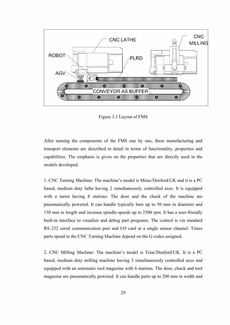
Figure 3.1 Layout of FMS
After naming the components of the FMS one by one, these manufacturing and
transport elements are described in detail in terms of functionality, properties and
capabilities. The emphasis is given on the properties that are directly used in the
models developed.
1. CNC Turning Machine: The machine’s model is Mirac/Denford/UK and it is a PC
based, medium duty lathe having 2 simultaneously controlled axes. It is equipped
with a turret having 8 stations. The door and the chuck of the machine are
pneumatically powered. It can handle typically bars up to 50 mm in diameter and
150 mm in length and increase spindle speeds up to 2500 rpm. It has a user-friendly
built-in interface to visualize and debug part programs. The control is via standard
RS 232 serial communication port and I/O card at a single sensor channel. Times
parts spend in the CNC Turning Machine depend on the G codes assigned.
2. CNC Milling Machine: The machine’s model is Triac/Denford/UK. It is a PC
based, medium duty milling machine having 3 simultaneously controlled axes and
equipped with an automatic tool magazine with 6 stations. The door, chuck and tool
magazine are pneumatically powered. It can handle parts up to 200 mm in width and
29
500 mm in length and the spindle speeds can be increased up to 2500 rpm. It also has
a user friendly built-in interface to visualize and debug part programs. The control is
via standard RS 232 serial communication port and I/O card at a single sensor
channel. Times parts spend in the CNC Milling Machine depend on the G codes
assigned.
3. Closed Loop Buffer: The model of the conveyor is SKF/UK. It is a unidirectional,
constant speed, closed loop buffer having 14 cups. Typically, it can handle
cylindrical parts up to 50 mm in diameter. It is driven by a motor with gearbox. The
control is via 48 channel I/O card. The conveyor has one operate channel and one
counter channel. When the operate channel is ON, it starts to rotate and stops when
the channel is OFF, the counter channel is used to count the cups passed. The
conveyor has a speed of 87 mm/sec and a total length of about 7100 mm’s. As a
consequence it makes a full rotation in about 82 seconds.
4. Robot: The robot is a Movemaster EX/Mitsubishi/Japan. It is a 6 axis controlled
material handling robot. The robot is capable of handling bars of 50 mm in diameter
and has a weight of approximately 3 kg’s. The control of the robot is realized by
storing positions taught by the user in its EPROM and these programmed positions
can be executed by external triggering of program commands through RS232
connection from the computer. ADSR (data set ready) signal from the serial port
indicates that there is no active program running or the task is finished. Each
operation carried out by the robot such as loading or unloading of machines and
conveyor lasts approximately 30 seconds.
5. Pneumatic Linear Robot Drive (PLRD): The PLRD is a product of
FESTO/Germany. It acts as a pneumatically powered linear drive for the robot and
has a movement range of 2 meters. The only stop positions of the PLRD are at both
ends only. In METUCIM configuration it is used to move the robot from CNC
Turning to CNC Milling neighborhood. The control is via 48 channel I/O card. The
PLRD has two operate- and two sensor channels. When the first operate channel is
30

triggered and immediately released it moves to right and vice versa for the second.
Sensor channels on the left- and right positions indicate ON when the robot is at left
and right ends of its range respectively. The traversing speed of the robot is not
constant during the 2 meter movement as it accelerates during starting and stopping,
keeping this fact in mind an assumption is made taking an average time for the robot
motion on PLRD, the motion is assumed to last a constant time of 5 seconds.
6. Static Buffer (AGV): The stationary buffer is used to import parts to the cell and
export the finished parts. It has 3 input and 3 output stations which can handle bars
of 70-90-100 millimeters. Actually, the buffer is not physically connected or driven
by a computer and it has no control or moving capabilities, however it is modeled as
an AGV in the system.
Figures B.2-B.5 in Appendix B are dedicated to the photographs of the components
of the system that show these components one by one. In addition to those
photographs, a photograph that shows the entire system when it is in operation is
provided as well in Figure B.1.
3.2 Simulation Structure
Systems to be simulated are quite diverse in terms of size and complexity. However,
regardless of how complex a discrete-event system may be, it is likely to contain
some basic components that are also common to flexible manufacturing systems.
The structural components of a discrete-event simulation include entities, activities
and events, resources, global variables, a random number generator, a calendar,
statistics collectors and animation (Ingalls 2001). These structural elements and their
relations with flexible manufacturing systems are described in the following
sections. The models generated throughout the study are used as examples to
demonstrate the methods of application for modeling and simulation.
31

3.2.1 Entities
The most essential elements of a simulation are the entities that move around
dynamically and cause changes in the state of the simulation. The changes are
generated through altering the resources, affecting or being affected by other entities
or by entering or leaving the system. Without entities, nothing would happen in a
simulation.
There are two possible types of entities, referred to as external entities and internal
entities (Schriber 2001). External entities are those whose creation and movement is
explicitly arranged for by the modeler. This type of entities usually has a “real”
equivalent in the system to be simulated. In our case, examples to this type of entities
are the parts to be processed. There exist several types of parts, explained in detail in
Appendix E requiring different processing and routing, which have different
properties assigned to them. In FMS, the most common external entities are those
that correspond to parts to be entered into the system.
In contrast to the external entities, internal entities are created and manipulated
implicitly by the simulation software itself or designed by the modeler to take care of
certain modeling operations. They may be used to account for logic operations
within the system such as changing the state of a resource at some certain time (e.g. a
machine failure, a capacity increase due to a shift). In our study an internal dummy
entity is created in the file reading and writing module to create a continuous loop to
keep on reading entity arrival times and properties from a text file.
Most of the programming effort required to account for logic operations using
internal entities in simulation, has been transferred to simulation packages with the
use of advanced simulation tools. Specially tailored built-in modeling constructs
used in ARENA® such as the modules named Failure and Schedule are examples to
internal entity creating modules.
32

3.2.2 Attributes
Entities retrieve their unique identities with the attached attributes to them. Perfect
analogous objects in literature to attributes are the adjectives. An attribute is a
common characteristic of the same type of entities, but with different values
assigned, they can differ from one entity to another, distinguishing one entity of a
type from another. These assigned values of attributes provide the basis to calculate
statistics and also offer programming flexibilities for the modeler.
The most important thing to remember about attributes is that their values are tied to
specific entities. These values can be assigned to entities at the beginning of a run or,
they can be assigned at special times during model run. The assigned values for
attributes are subject to change as the simulation run progresses and these values can
be used at any time during the run or even after the simulation run is complete.
The list of attributes used in simulation of the pilot FMS and their brief purpose of
usage in the developed models is given in Table 3.1. This table gives an essential
idea on the use of attributes and provides the modeler with a list to start with for
modeling a FMS. It should be noted that several other attributes may exist depending
on the complexity and specialty of the FMS to be modeled and depending on the
modeler and his/her programming skills..
The last column of the table is reserved to the type of the attribute used. The
attributes, although they belong to the same group in terms of simulation structure,
can have different application areas according to the purpose of assignment. In this
study attributes are collected under four main types as statistical, program, animation
and fundamental attributes. These attribute types are described in detail, in the
following paragraphs.
33

Table 3.1 The attributes used in the system, their brief descriptions and types. (Anim
stands for Animation, Fund for fundamental, Pro for Program and Stat for Statistical)
Name of Attribute Description Type
Check Operation
Traces the completion of individual machining operations
Pro
DueDate The parts due date is assigned to this attribute Fund
Entity.Picture The pictures used in the animation are assigned to this attribute
Anim
Entity.Sequence The entity follows the sequence defined in this attribute Fund
JOBFINISHED Traces the completion of all operations of the part within the system
Pro
Milling Time The Value of Milling Time is assigned to this attribute Fund
MilStart Marks the starting time of milling operation Stat
Part Index Part Type is assigned to this attribute Fund
Timein Marks the entities entry time into the system Stat
Turning Time The Value of Turning Time is assigned to this attribute Fund
TurnStart Marks the starting time of turning operation Stat
Statistical attributes are the ones that constitute the elementary basis for statistics
collection. Statistics such as average machining times or time in system are
calculated using each entity’s corresponding values. These values are assigned in the
following way. Before an entity is on the verge of a specific action in simulation
(entering a queue, start being conveyed, being grabbed by a transporter, or at the
initiation of machining, etc.), the entry time is marked to an attribute. ARENA® has
a built-in variable called TNOW, which returns the current simulation time. A
sample assignment code and the idea behind are demonstrated in Figure 3.2.
34

Figu
oper
corr
Upo
attac
actio
show
a)
re 3.2 At
ation b)
esponding
n comple
hed attrib
n, which
s the ass
)
; M; 32$
b
odel statements for module: Assign 22
c)tribute assignment for statistical purposes a) assign block before turning
assignment of the current time to the attribute TurnStart c)
SIMAN code.
tion of the related task, the time is recorded and using the previously
ute, a new attribute is assigned that has the information of the required
will be used at the end of the run for statistics collection. Figure 3.3
ignment code at this stage.
ASSIGN: TurnStart=TNOW:NEXT(49$);
35

a)
)
Figure
time u
corres
Funda
The in
usuall
inform
planni
part m
genera
the sim
Progra
model
a simu
Usual
Then
fundam
progra
; Model statements for module: Assign 20
b
3.3 Attribute assignment after completion of a task a) Assignment of Turning
sing current simulation time and the previously assigned attribute TurnStart b)
ponding SIMAN code.
mental attributes offer the means to attach basic information to the entities.
formation that is carried by this type of entities is known beforehand and is not
y subject to change during the simulation run. Attributes that store the
ation of machining times, part types, colors, features and other production
ng related predefined data such as sequences, costs, priorities, due dates and
achine relations are in this group. The assignments on this type of entities are
lly done at the beginning of the run, as soon as the newly created entity enters
ulation model.
m entities are used in simulation to offer some modeling flexibilities to the
er. It is not always easy to mimic the unique properties of the real system with
lation and modeling language as it is with general programming languages.
ly the modeler is forced to use branches to compensate for the entity related If-
structures and the variable used within the structure is either a program or a
ental attribute. An application of branching in the simulation by the use of a
m entity is shown in Figure 3.4. An entity that arrives in the Robot Exit
; 30$ ASSIGN: Turning Time=Turning Time + TNOW-TurnStart:
36

Station is first assigned a global variable, and afterwards it is either sent to the
conveyor to seize a place or the conveyor is stopped for the entity to leave according
to the value of the program attribute JOBFINISHED. This attribute has an initial
value of “0” at the beginning of the simulation and after the completion of all
manufacturing operations on the part the value is incremented to “1”.
Figure 3.4 Functional usage of program attributes
The last group of attributes is the Animation Attributes. As the name implies, these
entities are used to represent the pictures of the entities. These pictures are subject to
change as the part gets machined within the system. In the pilot simulated system,
Entity.Picture, the internal variable of ARENA®, is used to assign the pictures of the
entities.
In addition to the ones listed above, ARENA® keeps track of some attributes
automatically, to calculate its own statistics. Priorities and incurred costs to produce
parts can also be taken into account in FMS and attributes about them can also be
assigned to entities.
37

3.2.3 Activities and Events
Activities are the processes and logic that are defined in the simulated system.
Entities that interact with the activities constitute events and cause changes in the
state of the system. There are mainly three types of activities defined for simulation;
delays, queues and logic.
Delays are due to the detaining of the entities for a definite amount of time in the
systems. The length of this waiting time is either fixed or randomly generated by
using statistical distributions. The events related to a delay occur at the beginning
and the end of the delay, where the entity arrives at and leaves from the delay block.
An entity that successfully seizes a resource undergoes a delay, so it can be told that
every type of activity in an FMS that require a resource results in a delay. These
delay activities include but are not limited to machining, storage, inspection, and
transfers in FMS.
In the pilot application, delays are due to the processes defined in the system (turning
and milling) and the transferring of entities from one station to another (robot
loading and unloading). Robot loading and unloading delay is treated as a constant
value as it does not change from one part type to another, whereas the machining
times are taken from different triangular distributions for each type of part,
considering a pessimistic, optimistic and most likely time. This approach can be
modified considering fixed times for machining operations, as in FMS the
uncertainty in machining times is lower when compared to conventional machining
systems.
Queues also make the entities wait but the main difference from delays is that the
waiting period is unknown in advance. Waitings in queues mainly occur in one of
the following two conditions: Either waiting to seize for a resource, or waiting for a
system condition to occur such as storing the parts to be taken out of the queue when
38

the right conditions exist. Queues can have capacities representing a limited buffer
capacity.
In FMS, queues have also an important role on determining the production
philosophy. Queue selection rules are utilized to select parts from queues to
determine the next part that will get service from the available resources. In the pilot
FMS simulation queues that reflect the properties of both types of queues exist. The
queue WAIT FOR BATCHING.Queue is an infinite hold type queue and the entities
are forced to wait until a number of five finished parts in the queue exist. This type
of operation does not really exist in the existing FMS but added for demonstration
purposes for packaging applications and condition type queues.
Considering the queues that occur because of competing parts for resources, there
are many examples in the pilot FMS system. However, due to the nature of the
conveyor utilized in the system, queues that have capacities larger than 1 arise either
to seize a space in the conveyor or to be grabbed by the robot to enter the system. So,
the only real queue is the WAIT FOR SYSTEM.Queue that is for the entrance of the
parts to the system. For the other queues, the conveyor itself works as a buffer that
has a capacity of 14 and each part that is able to ask for being machined by the
turning or milling machines have no competing rivals waiting in the same queue as
the capacity of the conveyor at turning and milling stations is only 1.
Finally, logic activities allow the entities to help carry out decisions in order to
follow specific routes in the system. By interacting with the system state variables
and user defined variables and attributes, several logic operations can be realized.
The decision stages in the flowcharts can be directly transferred into simulation
models once the flowchart of the operations within the flexible manufacturing
system is determined. In addition to the logic operations that originate from the
flowcharts, logic activities can arise due to modeling necessities such as statistics
collection and attribute assignment.
39

In our pilot implementation, several examples to logic activities exist in every
sample model. Figure 3.4 in the previous section shows a logic activity in addition to
the functional application of attributes. Another equally important application of
logic activities is considering the system state variables. In the logic activity
demonstrated in Figure 3.5 the number of entities in WAIT FOR BATCHING.Queue
is used to collect a number of five entities for batching. The parts that arrive in the
Branch block are transferred in to WAIT FOR BATCHING.Queue until the number
of parts in the queue is 4. The next entity that arrives in the queue is used to remove
the entities in the queue in order to let the parts proceed within the model for
batching purposes.
Figure 3.5 Logic activities using system state variables
Similarly, branching operations in models due to assignments of specific attributes to
parts and statistics collection are also present in models. Picture assignment
according to part type and type of manufacturing process completed is realized by
branching and also statistics collection that is consistent with the type of completed
operations makes use of this logic approach.
40

3.2.4 Resources
In simulation, resources represent service providers with restricted capacity for
whom the entities compete with each other. Considering FMS’s, the extent of the
things that the term represents, contract to mainly machinery and equipment,
personnel or space in a storage area of a limited size. The resources are allocated to
entities when an entity successfully seizes that resource and released when the
required operations are finished.
An entity can seize more than one resource at the same time and also a single
resource can represent a group of several individual servers and can serve many
entities. An example to the first case is a part that seizes both a machine and an
operator at the same time. A machine or an area that has a capacity of more than one
is an example to the latter case. In addition to machines and operators, material
handling devices act like resources in the simulation of FMS. Conveyors, automated
guided vehicles (AGV) and other transporters are among the complex resources that
generally exist in FMS.
Several resources are used in the pilot simulation considering the real system and
possible alternatives to the existing configuration. Evidently, the main resources
simulated in the study are the existing CNC turning and milling machines. They have
a fixed capacity of one part for servicing and assumed to work without problems
except randomly determined breakdowns. The machining times of the parts are
determined considering the part types and the idle/busy times of the machines are
animated and discriminated with changing color of the lights above them.
One other resource in the system is the conveyor. It is modeled considering its
original speed, its 14 spaces for part storage and transport. The segments of the
conveyor are defined according to the distances between loading, unloading and
machining stations. The other resource is the robot that is modeled as a transporter.
This mobile robot is analogous to many AGV’s that possibly exist in any FMS. It is
41

modeled considering the distance it moves between the two loading stations and the
loading and unloading actions from the stationary buffer to the conveyor, from
conveyor to the machines, from machines to conveyor and from the conveyor to the
buffer.
3.2.5 Global Variables
Variables are the means to store information that reflects some characteristic of the
simulated system. They are used to track just about anything that is of interest to the
entire simulation. Coarsely, three usage areas can be defined for variables. The
modeler can define system state variables to control the entity flow and guide
simulation (Control variables) as well as to collect information on addressing certain
areas (Information variables). Besides, values that are subject to change during a
simulation run can be assigned to variables and this provides ease of access and
manipulation (Access Variables).
In addition to the user defined variables regarding the state of the system, the
simulation software itself usually keeps track of various variables. Average,
maximum and minimum values of attributes, numbers in queues and simulation
clock are examples to the variables internally kept by ARENA®. Considering such
similarities between attributes and variables, one question may arise at this stage,
about the difference of attributes from variables. The main difference is that
variables return the values, which pertain to the system as a whole, whereas
attributes carry entity specific information.
Once FMS are considered, there is no distinctive difference from other simulation
environments about the use of global variables. Variables used in the pilot study will
give a basic idea for advanced applications. Table 3.2 shows examples to each type
of variables used and brief descriptions. These variables are selected from different
models generated to provide an idea on application methods.
42

Table 3.2 Variables used in the system, their brief descriptions and types. (Acc stands for Access, Con for Control, Inf for Information) Name of Variable Description Type
Robot Transfer The time that loading and unloading action takes place is assigned to this variable
Acc
STATESYS It is a control variable that indicates that there is at least one entity in the system. The variable is used to accept entities when there is no part being processed in the system.
Con
Number in AGV Traces the number of waiting entities in the stationary buffer.
Inf
Scancontrol Traces whether there is an active entity seizing for a free space in the conveyor and robot
Con
Max Conveyor Traces the position of the parts on the conveyor Inf
Station2,10,11,15…
Traces whether there exists an entity in the associated station or not
Con
removed The value assigned to this variable determines the entity to be removed from the conveyor animation
Con
i Incremental counter Con
Variables are usually just numbers, however according to the requirements of the
modelers, vectors or even matrices can be assigned as variables.
3.2.6 Random Number Generator
A simulation study usually depends on random variables rather than pre-defined well
known events. Most of the processing times, entity arrivals and transfer times are
taken from statistical distributions and also machine failures are assumed to occur
randomly. In order to carry out these statistical procedures, each simulation package
has an internal software routine that generates a random number between 0 and 1
that is used in sampling random distributions, which is called a random number
43

generator. Everything that is random in a simulation uses the random number
generator as an input to determine values.
Today’s simulation packages have their own random number generators. ARENA®
has its own random number generator as well. The program has 10 built in random
number streams and lets the user use any of them or define his/her own.
3.2.7 Event Calendar
The calendar keeps a list of the events that are scheduled to occur in the future. The
detail of the event calendar’s data structure is of no interest when this thesis is
concerned, but it should be noted that when the logic of simulation calls for it, a
record of information for a future event is placed in the event calendar. One other
importance of event calendar is that the simulation clock is updated according to the
events at the calendar, rather than flowing continuously. Finally, it is worth
mentioning that it is an ending condition for a simulation run when there are no
events remaining in the event calendar and event calendar is kept internally by
ARENA®.
3.2.8 Statistics Collectors
The most tangible outputs of a simulation study are the statistical outputs as output
performance measures. A modeler should keep track of several statistical-collector
variables as the simulation progresses to come up with the necessary outputs at the
end. There are three different types of statistics, namely counters, time-persistent
statistics and tallies. Table 3.3 as a list addresses the statistic collectors defined
within the models, their brief descriptions and types. It should be noted that
ARENA® itself keeps track of almost any statistics available in the model; however
it is burdensome to select the required statistics among thousands of available ones
in a middle sized model.
44

Table 3.3 The list of the statistics collected, their brief descriptions and types (Cnt stands for Counters, Per for Time-persistent statistics and Tal for Tallies)
Name of Statistics Description Type
NumberOut1..4 Counts the number of parts of each type Cnt
Turning Scheduled Counts the number of times the turning machine is scheduled.
Cnt
Milling Scheduled Counts the number of times the milling machine is scheduled.
Cnt
Robot Scheduled Counts the number of times the robot is scheduled. Cnt
No of Batches Counts the number of batches produced Cnt
Timeinsystem Traces the time parts spend in system Tal
Lateness Traces the lateness of parts Tal
Earliness Traces the earliness of parts Tal
Turning Times Traces durations of turning operations Tal
Milling Times Traces durations of milling operations Tal
Machining Times Traces durations of total machining operations Tal
Turning Utilization Measures the utilization of turning machine Per
Milling Utilization Measures the utilization of milling machine Per
Conveyor Utilization Measures the utilization of the conveyor Per
Robot Utilization Measures the utilization of the robot Per
Number in AGV Measures the number of waiting entities in the AGV Per
Counters, as the name implies, are used to count occasions of a specific event. In
FMS, number of parts produced in a given time period and/or at a given cell is
usually of interest. The number of occurrence of specific events such as failures of
45

machinery or number of schedules of equipment also needs attention. Initially the
counters are set to 0 and these counters are updated on relevant occasions.
Figure 3.6 demonstrates the use of counters. A counter block is placed at the desired
point of counting in the model, before the disposal of entities to count part types at
this case. The specified counter ID is incremented according to the specified value.
As seen in the figure, Part Index is assigned to counter ID. Actually Part Index is an
attribute that takes values from 1 to 4 according to the part type. The counter
corresponding to the Part Index is incremented, which corresponds to counting each
part separately under different counters.
Figure 3
)
b
a)
.6 Statistics collection using counters. a) Count block in the model b) Details of count block
46

Time persistent statistics are those that give the time weighted values of some
variables in the simulation. The representation of these statistics involves the area
under a plotted curve, time being on the x axis, which is an integral representation. In
FMS utilizations of machinery and workers and also the number of entities waiting
in queues are included under this type of statistics.
Time persistent statistics are kept externally in the model using DStats element of
ARENA®. The simulation software has built in operands to calculate variables
regarding resources and queues. In Figure 3.7 the full list of the statistics kept is
given. The operands that calculate the time persistent statistics can be seen under the
DStats Element.
Figure 3.7 Statistics calculated in the simulated system with the addition of the operands of DStats Element
The first four address the utilizations of milling and turning machines, conveyor and
the robot respectively. The last line under the DStats element is for the number in
queue for two queues, which in reality refers to the number of parts on AGV.
Tally statistics are created using the values collected at single occasions from taking
the average, minimum or maximum of a list of numbers (usually attributes) without
47

regard to the time between the observations. The statistics are usually the times spent
during various events such as time spent in system, on machinery and material
handling devices or waiting in a specific queue. Other time related statistics such as
earliness and lateness are also of concern.
3.2.9 Animation
Animation in simulation of FMS is excellent for communication and adding
realization to models and it can also be used to debug the simulation program.
Validation of simulation models usually require a well set up animation component
for the modeler to observe the responses of the model to extreme conditions.
Animation can be divided into two main headings as animation of processes and
animation of statistics. Both are important in terms of helping the decision makers
grab the necessary outcomes out of the simulation study.
The amount of time and effort decided to invest on animation depends on the level of
detail required. However, FMS necessitate a sounder animation component when
compared to other systems because of the autonomy they involve. In ARENA,
animations can be created by several methods. ARENA has its own graphic tools,
and built in pictures to be assigned to entities and resources and also, animation
medium of ARENA accepts exported pictures and drawings to be used as
background images.
In Figure 3.8 a screenshot from the animation of one of the models is given. The
states of the robot, conveyor and the machines can be traced from the instant. Also
the positions of the existing parts in the system are clearly defined. There are 4 parts
of 2 different types in the stationary buffer waiting for station 10 to be emptied to be
able to enter the conveyor. There is a part being machined on the milling machine
and a finished part in the AGV in addition to one positioned on the conveyor. The
robot and the conveyor are stationary at the moment the capture is taken. A green
light on the machine indicates that it is busy whereas a red light indicates that it is
idle. Simulation clock is also added to the animation for ease of tracing time.
48

Figure 3.8 A screenshot from the animation
The significance of the collection of statistics was well discussed before in Section
3.2.8. In addition to the acquisition of statistics at the end of runs, the tracing of the
intermediate values of these statistics is of equal importance to identify the exact
characteristics of the system. ARENA® provides various animation options for
concurrent display of model statistics as the simulation run progresses.
In the pilot study, each model has an animation component that shows mentioned
statistics dynamically. Dynamic plots are used to show time-persistent statistics such
as number in queues, time being in the x axis. Utilizations are demonstrated with
levels. Histograms are applied to tallies and counters are visualized. Sample results
on the animation screen of statistics are demonstrated on Appendix A on Figures A-1
and A-2 with other simulation results.
49

3.3 Model development
In this study, ARENA® Simulation Tool is used to develop models. The capabilities
of the software, discussed in Chapter 2, are utilized effectively to come up with
models that are as realistic as possible. The flowchart of events given in Appendix F
is used as a guide for model preparation. During model verification stage, each step
of the execution has been traced extensively using both the ARENA®’s and Visual
Basic®’s interactive debuggers and the detected errors in the models and modeling
logic have been removed.
The generated models are different in terms of queuing methodologies however the
structures of the developed models are common up to some extent. The submodels
developed to construct the entire model are part creation, routing and assignment,
AGV loading/unloading, selection rule, machining operations, stations, part disposal
and data. Each submodel is discussed in the following sections and the modules and
blocks of ARENA that are used to develop these sub models are provided as
screenshot views in Appendix C.
3.3.1 Part Creation Submodel
The Part Creation submodel is responsible for the introduction of the parts to the
models. The nature of this submodel is arranged so that it allows the selection of part
arrivals either from a statistical distribution or from a Microsoft EXCEL® file. The
selection procedure will be discussed in detail in Section 4.2 when describing the
import data module.
In the first option the parts are generated from an exponential distribution of with a
mean value of 5 minutes. This value may seem unrealistic when the nature of the
FMS in hand is considered as it is not used intermittently; however if it were to be
used continuously with work orders following one another, the parts that arrive in
this time intervals would result in a steady state system. A creation limit of 180 parts
50

is used, limiting the number of parts to arrive at the system for a day. The ASSIGN
block next to the CREATE block is used to assign the attributes such as due dates
and part indexes, to identify the created part.
The second option at this stage is letting the user use the values entered to an
EXCEL® file as part arrival data. A single control entity is generated at the
beginning of the simulation if this option is selected. This entity is responsible for
reading the values of part arrival times, the associated part indexes, due dates and
priorities. The duplicated entity enters the system with attached data and the control
entity keeps on looping until the last part data. Once the last line of data is input from
the file, the control entity is disposed. Figure C.1 shows the submodel’s blocks and
modules.
3.3.2 Routing and Assignment Submodel
As the name implies, routing submodel is responsible for routing the parts that arrive
or that are expected to arrive at the AGV station. Firstly, the assignments are made
providing the part with some values necessary for simulation. Next, it is decided
whether the part is a new part that is trying to leave the AGV or whether it is a part
trying to reach AGV. According to the decision, if the part has just entered the
system, the position of the furthermost entity on the conveyor is checked and if there
is a free space in the conveyor the status of the conveyor is set to available and the
part is transferred to a queue where the selection from the queue depends on the
utilized selection rule. The duplicated entity leaves the submodel to trigger the
selection rule submodel. The part that returns through selection submodel seizes the
robot and is sent to loading and unloading AGV submodel.
The other possibility for a part to enter the routing submodel is a part that is to leave
the system to be stored in the AGV. After realizing that the part is to leave the
conveyor for AGV, the part is removed from the conveyor and sent for part disposal
submodel.
51

3.3.3 Selection Rule Submodel
For most of the models, there is a selection rule submodel that is used to pick up
parts from the waiting queue according to the desired production philosophy. The
duplicated entity in routing module is used to search within the queue. The part that
satisfies the search condition (i.e. earliest due date, longest processing time, etc.) is
sent back to the routing module and initially duplicated entity is disposed. Figure C.3
demonstrates the submodel.
3.3.4 AGV Loading and Unloading Submodel
This submodel shown in Figure C.7 corresponds to the station 10 of the actual FMS
which is used for loading and unloading the AGV. A part can reach this submodel in
three occasions. A part that has recently entered the system that is sent through the
routing submodel, a part that has completed its operations and waiting to leave for
AGV or a part that has first entered the milling station and passing through the
unloading station to be delivered to the turning station.
In the case of a finished part, the action to be taken is straightforward. Using the
Branch block, an entity whose JOBFINISHED attribute is set to 1 is sent to the
routing submodel. That part will further be sent to the job disposal submodel for
being removed from the system.
For the case of a new part, the part is allowed to seize a place on the conveyor. The
robot is freed after the part is allocated a place on the conveyor. The procedure after
is the same for the remaining case also. After making the assignments for station
numbers that determine the position of the parts, the availability of the robot and the
turning machine is scanned and when appropriate conditions exist, the part is sent to
the station depending on the sequence determined in Sequences element of ARENA®
as the part process plan.
52

3.3.5 Stations Submodels
The flow of the parts on the conveyor is controlled through effective usage of
stations. There are three station submodels controlling the positions of the parts on
the conveyor two of which are between turning and milling stations and one before
the loading / unloading station. At each station, the assignment regarding the position
of the part is made initially and when the appropriate conditions exist, the part is
conveyed to the station in sequence. Figures C. 4-5-6 show the associated modules
and blocks to model these stations.
3.3.6 Machining Operations Submodel
Machining submodels that comprise the turning and milling operations in the system
form the core of the developed models. The parts are delivered to this submodel
through other submodels and the sequence of the turning and milling operations
depend on the production plan of the part. Once all the operations are finished the
parts are directed to AGV loading and unloading submodel.
A part that arrives at the Turning Station in Machining operations submodel is
checked, considering the production plan and the completed operations after the
assignment of station numbers. The parts with a turning operation to be realized
initially request the robot, then they are delayed for unloading time. Next, they leave
the conveyor and access to the Turning Machine. The robot is freed and after the
operation that lasts according to the part type the assignment of work in process
pictures is done. After the seizing of the robot, the turning machine is released and
the part gains access to the conveyor. Finally, the robot is freed and the part is
conveyed for the operation in sequence.
In the developed models, milling station operations are similar to turning station
operations. The parts that arrive from the station submodels reach the milling station
and the parts that require milling are sent to milling routines. These routines are
almost the same as the turning routines, the only difference being the allocation of
53

milling machine instead of the turning machine. The parts that do not require milling
are sent to the stations in sequence in their production plan.
The routines of a part accessing and leaving the conveyor are included in the
submodel where necessary, to trace the parts on the conveyor and their locations.
Also counters are utilized in the submodel to count the number of schedules for the
machines and the robot.
3.3.7 Part Disposal Submodel
Once the parts complete operations in the machining operations submodel, and leave
the routing submodel to be disposed, part disposal submodel is in action. Firstly, the
statistics are collected according to part types, milling times are collected for only
milled parts, turning times are collected for only turned parts. Machining times are
collected for every part. Once the parts reach the Exit system station, time spent in
system for every part is calculated in addition to the lateness / earliness values.
Counters are utilized for counting the parts by part type and VBA codes are executed
to transfer these values into environmental applications, which is the subject of
Chapter 4.
The last operation done in the model is collecting the parts in to batches of 5 pieces
and disposing all the entities that represent the parts after counting them. Figure C.8
of Appendix C shows the submodel in modules and blocks.
3.3.8 Data Submodel
Data modules define the characteristics of various process elements, like entities,
resources, and queues. They can also set up variables and other types of numerical
values and expressions that pertain to the whole model. Icons for data modules in the
Project Bar look like little spreadsheets. The Basic Process panel's data modules are
Entity, Queue, Resource, Variable, Schedule, and Set; the Advanced Transfer panel
includes Sequence, Conveyor, Segment, Transporter and Distance. Entities don't
54

flow through data modules, and data modules aren't dragged into the model window;
rather, data modules exist "behind the scenes" in a model to define different kinds of
values, expressions, and conditions.
The modules on the Advanced Transfer Panel are used to define the part process
sequences, conveyor and transporter properties such as the conveyor type, velocity
and cell and segment distances. The modules of the Basic Process Panel are used to
define entity types, queues and queue types, resources and capacities, initial values
of variables and part picture sets.
55
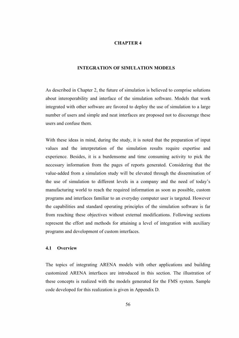
CHAPTER 4
4 INTEGRATION OF SIMULATION MODELS
As described in Chapter 2, the future of simulation is believed to comprise solutions
about interoperability and interface of the simulation software. Models that work
integrated with other software are favored to deploy the use of simulation to a large
number of users and simple and neat interfaces are proposed not to discourage these
users and confuse them.
With these ideas in mind, during the study, it is noted that the preparation of input
values and the interpretation of the simulation results require expertise and
experience. Besides, it is a burdensome and time consuming activity to pick the
necessary information from the pages of reports generated. Considering that the
value-added from a simulation study will be elevated through the dissemination of
the use of simulation to different levels in a company and the need of today’s
manufacturing world to reach the required information as soon as possible, custom
programs and interfaces familiar to an everyday computer user is targeted. However
the capabilities and standard operating principles of the simulation software is far
from reaching these objectives without external modifications. Following sections
represent the effort and methods for attaining a level of integration with auxiliary
programs and development of custom interfaces.
4.1 Overview
The topics of integrating ARENA models with other applications and building
customized ARENA interfaces are introduced in this section. The illustration of
these concepts is realized with the models generated for the FMS system. Sample
code developed for this realization is given in Appendix D.
56

The import data module presents a module in which scheduled arrival times, part
types, due dates and priorities are read from an external file. The set-up of the file,
communication means and data imports are discussed.
Export data module is for the formation of a report file in which several statistics are
presented in terms of charts and tables. The following context is dedicated to setting
up of the file, creation of the charts, modifications on the format of the files and data
exportation means.
Interface module presents the preparation and usage of custom interfaces to edit,
modify and change several parameters of models created. The discussions are about
the creation of forms and execution of controls on these forms.
VBA modules present the collection of statistics and exportation of these data to
files. The discussion about VBA modules is about the placing of these modules
inside the models created and the codes generated to achieve the collection of
required statistics.
All those mentioned modules are realized through two Microsoft® Windows®
operating system technologies that ARENA® exploits for integrating directly with
other programs, ActiveX® Automation and Visual Basic® for Applications (VBA).
For data access to a variety of data stores, as in the case of the import data module,
ActiveX® Data Objects (ADO), which is also a Microsoft technology, is used.
4.2 Import Data Module
The successful operation of an FMS starts with the work orders. There are several
methods to model these working orders, such as taking samples to determine the
statistical distribution behind and use random arrival times according to this
distribution, or letting the user of the model to input the required values. The models
57

developed throughout the study let the user select from these two options. The
selection procedure will be explained in detail in the following sections, but initially
the development of a user friendly import module is discussed.
The file reading operation in ARENA starts with the definition of the file to be
accessed in File Element in the Advanced Process Panel of ARENA. The name,
Access Type, Connection String and the Recordsets that the file possesses are
defined here as shown in Figure 4.1. Two different methods are proposed for reading
arrival data. First, data are read in from a text file that contains the Part Type, Time
of Arrival, Due Date and Priority information in rows separated by tabs. However,
considering the difficulty of preparing a file directly in the above format another
alternative is proposed.
Figure 4.1 The details of File element in advanced process panel
The same information is kept in an Excel® file with headings above each type of
information. The field that stores the data is kept as a Recordset and a Connection
String that allows data transfer between the file and the ARENA model. Figure 4.2
gives the ActiveX Data Objects (ADO) Connection String that allows the use of
Excel with the support of headings used in the developed models.
Figure 4.2 Connection string for Excel with headings using ADO
58

After the arrangement of the files element, it is necessary to adapt the file reading
and writing module into the developed model, which is a modeling concept rather
than integration. It should be noted that the Recordset ID specified in ReadWrite
module should be the same with the Recordset Name in the File element. Once an
entity passes from this module data in the Excel file under the headings will be
assigned to this entity’s specified attributes. Figure 4.3 shows the ReadWrite module.
Figure 4.3 The ReadWrite module to access the Import Data file
So far, the methods to communicate the model with the prepared Excel file are
discussed. In addition to the integration of ARENA and Excel, a program with an
interface that will help the user to submit work orders is prepared. This interface
shown in Figure 4.4 helps to create the necessary worksheet to be used directly by
ARENA® as a data source. The user can easily add new work orders using this
program or directly manipulate on the previously defined work orders by opening the
work sheet that stores the accompanying data.
59

Figure 4.4 Developed interface for worksheet preparation
The working principle of the program is as follows. The user enters the part type,
arrival time, due time and priority of the part to be entered to the model as a work
order following the instructions. Upon pressing the load button, entered data is taken
into the worksheet and a sorting operation is realized to sort the work orders in the
order of increasing arrival time. Clear all data button is used to clear all previous
work orders. The space above this button is reserved for messages. If any erroneous
data is entered in the cells, data cannot be loaded to the work sheet and an error
message of “Erroneous Data” appears. On the case of a successful loading of work
order data, “Data Loaded” message appears. The code developed for the realization
of above tasks is given in Appendix D
4.3 Export Data Module
Upon completion of simulation runs, ARENA® itself creates reports about almost
every component of the model, including resources, queues, attributes and variables
transporters, conveyors, etc. However, these reports are of hundreds of pages long
and although being classified under main headings by ARENA®, it is a tough task to
reach the required information in a small amount of time. The reports created by
ARENA® have deliverability, but it is not possible for the end users to manipulate on
those reports to make the necessary changes.
60

Creating customized outputs require programming efforts. For this purpose, the
export data module is created by Visual Basic applications with the utilization of
ARENA® Objects and ARENA®’s built-in VBA events. ARENA®’s built in VBA
events fall into three broad categories as pre-run events, ARENA-initiated run events
and model/user-initiated run events. However, most of the programming effort is
concentrated about the simulation run. Figure 4.5 shows the sequence of ARENA
actions and VBA events that occur with the start of a simulation run. This figure also
points out to an important aspect, regarding the type of data that are available for
VBA codes. According to these timing options components of the module are placed
as seen in the same figure.
Figure 4.5 Simulation-Run VBA events
The functioning of the data export module starts with the creation of an Excel file in
the ModelLogic_RunBeginSimulation event of ARENA. After the creation of the
file, worksheets to be used for data submission are created and the headers of each
61

page are prepared. Although the values for attributes are generated throughout a
simulation run, each worksheet is expected to have standard text values specified for
specific cells such as headers and identifiers. The assignments of these text values
are done at this stage, preparing the general layout of worksheets.
ModelLogic_RunBeginReplication event is used to create replication dependent
sheets to the previously created file. The formatting of these sheets is also done at
this stage. By formatting, the creation of row headings and definition of fonts and
number formats is meant.
As the simulation run progresses, the columns prepared beforehand, are filled with
the values that are transferred from the simulation run via VBA blocks. The details
of the VBA modules will be discussed in the following section.
After each replication run is completed, ModelLogic_RunEndReplication event is
called. At this stage the averages of the replication dependent values in columns are
calculated and charts are created that demonstrate the trends of the traced attributes.
Statistics that count on the DSTATS module of the ARENA® template (time-
persistent statistics) are also calculated at this stage and transferred into the prepared
sheets. Figure 4.6 shows one of the output charts of the data export module.
Time In System
0
20
40
60
80
100
1 6 11 16 21 26 31 36 41 46 51 56 61 66 71 76 81 86 91 96 101
Parts
Syst
em ti
mes
in
min
utes
Figure 4.6 Sample chart prepared by the program for data export module
62

As seen in the developed web pages on Figure 4.7, the export data module prints the
values of production related attributes of each part such as part type, priority, system
entrance time, exit time, time spent in system, the earliness or lateness according to
the due date, the individual turning and milling times and the total machining time.
In another worksheet, counter based statistics are printed out, such as the number of
parts produced, the number of schedules of turning and milling machines and the
robot. Resource, conveyor and robot utilizations and the average number in queue
for the AGV station are also provided in statistics worksheet. The other two
worksheets seen in the tabs are the charts dedicated to the Time in System and
Machining Times attribute values, similar to Figure 4.6.
Figure 4.7 The outputs from the Data Export Module
63

The idea presented here is that almost every statistics that is naturally kept by
ARENA® can also be externally calculated and presented to the end user with the
tools he/she is already familiar with. The modeler should specify the type and
amount of necessary information considering the needs of the end user and
customize the data export module accordingly.
4.4 VBA Modules
When a simulation run is started, ARENA® checks and initializes the model placing
the model in a run state. During the run, the values of variables, resource states,
statistics, etc. can be reached, examined and changed through ARENA®’s run
controller and through VBA codes. VBA codes can be utilized before, after and
during the run, according to the type of the tools used. As described before, the
timing of the events on the data export module was determined according to the
built-in events of ARENA®, however with the use of VBA modules the occurrence
of events is synchronized with special events in the simulation.
The VBA module operations in ARENA® start with the placement of a VBA block
inside the model on appropriate location. The place of the block determines the time
of execution of the associated VBA code. There are three VBA blocks associated
with each model in the developed simulation models. Figure 4.8 shows the
placement of one of the VBA modules inside the model. The VBA block is placed as
if it is one of the other modules or blocks with one enter and one exit point.
Figure 4.8 Placement of VBA blocks
64

The three VBA blocks are placed within the model for the updating of fields in the
excel worksheet created by the Data Export Module. The first VBA block is placed
at the system exit, where the parts leave the system. At this point, the
VBA_Block_1_Fire() procedure is called for each entity. This procedure is
responsible for inputting the values of the attributes of the part that passes through
the block to the corresponding fields on the Excel sheet named “Simulation Results”.
In addition to that the part numbers in “Statistics” sheet is incremented accordingly.
The other two VBA blocks are placed after a part is machined on one of the
machines to indicate the number of schedules of each machine. Whenever an entity
passes through the VBA module, the counter values kept in the simulation run are
transferred to the corresponding cells in the “Statistics” work sheet.
4.5 Interface Module
The necessity of development of custom interfaces for simulation was discussed on
several occasions before. The purpose of the interface module is to interact with the
users who are running ARENA® models, while allowing the user to make simple
manipulations without delving into the details of the model. Several kinds of
interfaces can be built providing the user with options to select from about the
general parameters of the simulation run or about specific data regarding the model.
Also, interfaces that let the user to interact with and modify the model on the
occurrence of specific occasions can be developed.
An interface that allows a choice to be made to use either part arrivals generated
from a random process or from a file when the model runs is developed to assess the
feasibility of the concept. Figure 4.9 shows the pop up window that is displayed at
the beginning of the run providing the options. The user selects the desired option by
clicking on the appropriate option button, then clicks OK button to allow the
simulation run to commence.
65

Figure 4.9 Part arrival interface
The first step for preparing this kind of an interface is to set up the model so that it
can perform all of the operations offered as options to the user. In other words, when
the developed interface is considered the model should be modified to generate
entities from both the random arrival process and the input file. The details of this
operation were described in Chapter 3 on the development of sub-models. The VBA
Userform is prepared as the second step, inserting the option and command buttons
and labels. The next step is writing the Visual Basic® code that runs according to
user’s choices and makes the changes on the modules in the model.
The timing of the interface is arranged according to the placement of the show option
for the form, frmArrivalTypeSelection.Show, for our case. The form can be
associated with VBA blocks in the model or with built-in ARENA® events. Part
Arrivals interface is functional at the start of a run so, it is displayed under the
ModelLogic_RunBegin event of ARENA®.
The idea presented here is that by the development of custom interface, the modeling
capabilities of an advanced modeler can be transferred to an average end user
through the use of programming techniques.
66

CHAPTER 5
5 TEST RUNS
In order to check the credibility of the developed models several runs are realized
under different scenarios. The results obtained after these runs provide a scientific
basis to evaluate the optimal sequencing algorithm for parts to enter the system. The
scenarios of the runs, run parameters used in the test runs, and the results of these
runs are described in the following paragraphs.
5.1 Test Scenarios
One of the main objectives of this work is to create a system that enables making
comparisons between different production philosophies. A specially tailored bidding
algorithm or a well known and easy to apply heuristic, each philosophy come with
its own advantages and disadvantages. Before being applied to the real system,
possible outcomes of the changes in scheduling philosophy can be seen in advance
of using the scenarios developed.
The agent based system in hand, as the name implies, uses agents to decide on the
sequence of the jobs. The algorithm used in the system for realizing the tasks is
called “bid preparation algorithm” and can be summarized as follows (Cangar 2000).
The customer agent identifies and announces a task to be done and criteria for bids.
The bidding server agents send bids for the announced task to the costumer agents.
The bid, satisfying the given criteria is awarded and the task is given to the selected
server.
The algorithm proposed is resource driven and operational if there are competing
resources (servers in agent terminology). With this in mind, one can realize that the
67

scheduling system do not take the properties of the work orders such as due dates or
parts with different process plans into consideration, and these work orders are
processed in the order of arrival.
An improved version of the algorithm contributed by Alataş (2003) can deal with
urgent work orders and the concept of assigned priorities is introduced. In this
method it is possible to reorder the compartments of the queue using these
properties. The parts with same priorities are dealt with the simple First Come First
Served (FCFS) rule.
The following sections are dedicated to the developed alternative scenarios for the
realization of a given production plan. These philosophies are discussed briefly and
application methods are discussed.
5.1.1 First Come Served
The simplest of all kinds, FCS (First Come Served), is considered as the first
alternative to provide a basis for comparisons. The philosophy is simple and
straightforward as the name implies; the first part to come to the system is served
first and the other parts are delayed until the completion of the tasks, or in other
words considering the purpose of our production system, FCS refers the one by one
processing of parts in the order of arrival.
FCS is applied in the system in the following manner. The first work order that
arrives in the Automated Guided Vehicle (AGV) triggers the system and the robot is
utilized to transfer the part to a free cell in the conveyor. The part is then processed
in the specified order according to the assigned process plan. The other parts that
belong to other work plans are kept in the AGV until the work order that is currently
processed is completed. After the completion of all the processes of the work order,
the part is conveyed to unloading station and the robot is finally utilized once again
to unload the part. The sequence is repeated until all the work orders waiting in the
68

AGV are processed. The first part to enter the system is decided according to the
order of arrival by AGV.
5.1.2 First Come First Served
The next alternative methodology to consider is First Come First Served (FCFS).
This philosophy differs from the previous one, from the point of allowance of
multiple numbers of parts in the system simultaneously. It indicates the policy of a
particular establishment to serve the parts in the order that they have arrived, without
other biases or preferences.
The application of FCFS to the simulation system is similar to FCS. The first work
order that arrives in the AGV triggers the system and the robot loads the part from
the AGV to the conveyor. When a new part arrives to the system at this time, that
part is also transferred considering the current state of the robot the conveyor and the
machines. The selection of the entering part among the parts waiting in the AGV is
realized by FCFS rule. The inherent properties of the Hold module of ARENA®,
directly selects parts accordingly.
5.1.3 Earliest Due Date
As another alternative methodology, due dates of the parts are considered. Earliest
Due Date (EDD) indicates the policy to accept the part with the earliest due date to
the system, without considering any other property of the parts. In EDD, multiple
numbers of parts are allowed in the system at the same time as in the case of FCFS.
The application of EDD to the simulation system is similar to FCFS. The first work
order that arrives in the AGV is directly taken into the system and the other parts that
arrive afterwards are temporarily kept in the AGV before being transferred to the
conveyor. The selection of the entering part among the parts waiting in the AGV is
realized by EDD rule. For this purpose a selection rule submodel is added to the
69

developed model to search among the parts waiting in the AGV for the part with the
earliest due date.
5.1.4 Longest and Shortest Process Times
Two other alternative methodologies consider the remaining process times of the
parts. Longest Process Times (LPT) and Shortest Process Times (SPT) indicate the
policy to accept parts according to the total time for turning and milling operations
with longest process time first and shortest process time first, respectively. SPT is
generally regarded as an efficient rule in that it tends to reduce average waiting time,
and hence average flow time.
The applications of LPT and SPT to the simulation system is similar to the
mentioned other methodologies. The parts waiting in the AGV are reordered as new
parts arrive in the cell, moving the parts with longest or shortest process times to the
front of the queue according to the selected rule. The submodel developed for EDD
case has been modified to account for selection of the appropriate parts with the
desired attribute.
5.1.5 Priority
Priority is a term that refers to precedence; that is the status established in order of
importance or urgency. Each work order comes with a defined priority value. The
work orders are queued according to their priority values so the part with higher
priority can be manufactured before the others. The queuing list is dynamic that, it is
updated by a decreasing priority, each time a new work order is added to the queuing
list.
The application of priority to the models requires the assignment of priorities to the
parts, before a part enters to the AGV. Then the work orders that are delayed in the
AGV are accepted to the system considering these assigned priority values, being the
70

part with the highest value the first. A modified version of the previously developed
selection rule submodel is used for this case as well.
5.2 Run Parameters
For each simulation run, it is necessary to define some parameters beforehand. These
parameters include, simulation dependent parameters such as run lengths, and model
dependent parameters such as arrival schedules and due dates. Different values
specified for these parameters can affect the outcomes from a study drastically.
5.2.1 Determination of Run Lengths
The system analyzed in this study is inherently a non-terminating system. In a non
terminating system, there is no event that causes the system to return a fixed initial
condition. Hence, there is no natural basis for selecting either the starting conditions
or the length of the runs.
For the cases of input data reading from prepared files, the run length phenomenon is
out of consideration as the simulation terminates when there are no existing entities
in the system, which is completely based on the number of parts given in the input
data files.
For the cases of input arrival times from statistical distributions a run length of 24
hours is specified, keeping the unmanned nature of FMS’s in mind. This value is
subject to change according to the modeling horizon and modeling objectives of
another FMS.
5.2.2 Determination of Arrival Schedules
As stated before in the preceding chapters, the models can accept two types of data
for part arrivals. Under operating conditions for the models, the data input for part
71

arrivals is expected from the user through the input data module; however for sample
runs a data input file is generated. The file includes 100 parts from different part
types with associated arrival times, due dates and priorities which are all created
randomly.
When part arrivals from statistical distributions case is concerned, one should carry
out statistical data analysis and distribution fitting techniques to obtain statistical
distributions to represent the patterns of part arrivals. However, when the working
principles of the modeled FMS are concerned it should be noted that the system
completely works on deterministic part arrival schemes under the consent of the
system administrators. So the selection of part arrival statistical distributions is done
considering the other model parameters taking into account the machining times of
the parts, not to end up with a system that will extensively be populated with parts
and contrarily, not to have a few parts traveling in the system. The exponential
distribution is used to model inter arrival times in random arrivals of parts with a
mean value of 10 minutes.
5.2.3 Determination of Due Dates
As in the case of part arrival times, due dates are also subject to two methods for
being attached to the parts that enter the system. Under normal operating conditions
the user inputs due date values together with the part arrival schedules using the data
input module. In the case of our runs the due dates are arranged according to a
Uniform distribution. A random number is selected between 0 and 100 and it is
added to the system entrance time of a part to be used as a due date. This value is
consistent with average times spent in systems and provides the basis for the
calculation of lateness and earliness values.
In the case of selecting arrivals from random distributions, due dates are calculated
in the same way as in the case of the sample test runs.
72

5.3 Run Results
Test runs are made by using the specified parameters in the preceding section. Part
process plans used in the runs are given in Appendix E. The statistical results of the
runs under 6 different scheduling algorithms are given on the following tables. Table
5.1 gives the average values for the selected performance measures. These values are
taken from the Export Data Module’s of the corresponding models. Further results
can be examined in Appendix A.
Table 5.1 Averages of performance measures. FCS FCFS EDD SPT LPT PRI.
(in minutes) TALLY VARIABLES
Lateness Value 66.261 48.517 34.492 36.571 56.545 39.800
Earliness Value 19.120 63.181 30.451 30.541 30.782 31.810
Turning Times 6.683 6.675 6.678 6.687 6.687 6.685
Milling Times 3.496 3.505 3.505 3.501 3.501 3.496
Machining Times 7.634 7.635 7.638 7.641 7.641 7.632
Time in System 102.830 56.814 57.897 57.094 75.363 63.518
Total Makespan 1236.55 1159.46 1157.99 1151.01 1155.15 1151.95
DISCRETE-CHANGE VARIABLES
Milling Utilization 0.212 0.255 0.253 0.256 0.254 0.254
Turning Utilization 0.405 0.442 0.445 0.447 0.449 0.448
Conveyor Utilization 0.020 0.227 0.237 0.236 0.258 0.223
Robot Utilization 0.243 0.331 0.324 0.333 0.333 0.334
Number in AGV 7.323 0.903 0.871 0.825 2.086 1.570
73
In addition to the average values of the performance measures, some of the statistics
are important from the point of number of occurrences such as the number of late
parts and early parts. Each delivers different costs to production, although it is out of
scope of this study.
Table 5.2 Number of occurrences for important performance measures. FCS FCFS EDD SPT LPT PRI.
TALLY VARIABLES
Lateness Value 85 41 60 57 65 57
Earliness Value 15 59 40 43 35 43
Additionally, the numbers of schedules for the robot and the turning and milling
machines is important. The scheduling of the components can incur fixed costs and
from maintenance point of view they need to be traced. As the number of parts and
their respective plans are same for all the scenarios these values are also the same for
all runs.
Table 5.3 Number of schedules for hardware components. Turning Machine Milling Machine Robot.
Number Scheduled 75 75 500
Some statistics are important considering the resulting maximum values. The
maximum time parts spend in system and the maximum lateness values are
important for tracing the system performance and the maximum number of parts on
the AGV is important to define the incoming part capacity for the static buffer.
74

Table 5.4 Maximum values for important performance measures. FCS FCFS EDD SPT LPT PRI.
(in minutes) TALLY VARIABLES
Lateness Value 138.52 138.39 109.79 168.14 285.37 153.00
Time in System 154.28 163.71 170.12 225.33 297.06 246.53
DISCRETE-CHANGE VARIABLES
Number in AGV 12 6 6 5 10 13
More of the results obtained are provided in Appendix A as they are prepared in
export data module. In these demonstrative test runs of the developed models it is
observed that the results obtained can be used effectively to decide on the parameters
of the FMS both in terms of hardware components and production philosophies.
Sample comments depending on these results are as follows:
When the tardiness values are concerned it is observed that the EDD principle
provides the minimum average for lateness values, which is an expected result. The
long waiting times in SPT and LPT algorithms increase the time in system values for
specific part types, which in turn increases the lateness values. The “only one part in
system” principle of FCS results in elevated values for all time dependent statistics
except earliness values. The use of EDD does not guarantee the minimum number of
tardy jobs. This fact is seen on Table 5.2 as the minimum number of tardy jobs is
attained in the FCFS rule. This is not a surprising result as the due dates are
dependent on the system entrance time.
Turning, milling and consequently the machining times are almost equal for all
sample runs as the part numbers and types used in all the runs are the same. The
importance of this statistics arises when the total manufacturing times are compared
with makespans of the parts. In the best configuration that minimizes the time in
75

system of the parts, FCFS rule, the average manufacturing time is about 14% of the
average makespan of the parts. In the most unfortunate case this value drops to about
7.5 %. The effect of this fact demonstrates itself through low utilizations of
machines.
The utilization of turning and milling machines are about 45% and 25% respectively
and do not differ in significant amounts from one scenario to another. This is also an
expected result, as the scenarios directly affect the system entrance sequences for
parts and there is no machine dependent sequencing. Another fact identified through
these utilization and machining times values is that the system is highly
transportation and storage means dependent as most of the time parts spend in the
system are due to waiting on the conveyor.
The number in AGV statistic is important to identify the AGV capacity. As
expected, The FCS scenario results in the most number of both average and
maximum parts on the AGV as only one part is accepted into the system. The LPT
and priority scenarios also cause elevated number of parts waiting on AGV as less
prior parts or, parts with short processing times are forced to stay on the AGV for
long times. The maximum number of parts on AGV is also important as the capacity
is directly dependent on this value. The SPT scenario results in the least number of
both maximum and average entities on AGV.
It is obvious that the results obtained are production order dependent and are subject
to change. Considering all those results, an objective function can be determined
according to the requirements of the management of the FMS. Before realizing the
production orders on the actual FMS, these orders can be processed on the models
and according to the results of the runs a production scheme can be figured out.
76
CHAPTER 6
6 CONCLUSION AND FUTURE WORKS
This research on Computer Integrated Manufacturing is mainly focused on the
implementation of a flexible, re-configurable simulation and modeling system. It
focuses on realizing the modeling and simulation of Flexible Manufacturing Systems
by the use of the hardware in Middle East Technical University, Mechanical
Engineering Department, Computer Integrated Manufacturing Laboratory
(METUCIM), Ankara, Turkey as a test-bed. In addition to that, the means of
integration of simulation with auxiliary programs is demonstrated. The models
developed throughout the study are used to come up with different scenarios of
production and sample results and decisions about production issues that can be
attained through the use of simulation are provided.
Simulation has historically found a great deal of applications in FMS’s. The need of
simulation arises with the questions to be answered when planning of an FMS at the
design or operation stages. As it can be seen in the outline of the thesis; the first part
of this study deals with the identification and implementation of structural simulation
components on FMS. These components are defined and explained in detail by the
use of examples taken from the developed models. Subsequently, the model
development procedure is explained with the introduction of sub-models. These
concepts are important to provide a guideline for the development of simulation
models for other FMS’s.
Simulation is expected to increase its strength and area of application through
integration with other tools. These other tools will include spreadsheets, statistical
analysis software, mathematical optimizers, programmable logic designers, robotic
77

software, or process flow layout and analysis tools. With this motivation in mind, the
scope of the work is extended to comprise the development of methods and
applications to be used for linking a simulation package, ARENA®, to less advanced
programs such as text editors and Microsoft Office® programs with the development
of custom interfaces to provide a fast and effective decision support tool for every
level of a company. This combination provides the users with a tool that is fast to use
and easy to maintain for the assessment of performance measures for FMS.
The actual aim to be expected from a simulation study is its supplying a scientific
basis for making decisions about the modeled system. The developed software
provides the infrastructure and it is the management’s task to analyze the results and
respond to the facts of the system. As the final component of the study, sample
simulation runs under different scenarios of production are presented. The
preparation procedure of the runs and the interpretation of the results obtained
through the developed software are important to provide an idea on the effective use
of simulation in manufacturing systems.
The scope of the thesis comprises both a modeling and application approach. It
provides guidelines on the determination of modeling parameters for FMS and
integration of the models with other programs. Although attentive work is employed
on the subject, the approach has certain limitations and drawbacks. These can be
summarized as:
The results of the models can not be directly verified with the existing agent
based system as the system is limited considering the number of work orders
that can be processed at the same time. The verification is done by comparing
the responses of the system with the responses of the models.
The bidding times those contribute to the overall systems times in the actual
FMS are neglected through the modeling approaches. Actually the response
of the system under heavy work loads is unpredictable due to computer crash
78

problems. So bidding times that contribute to less than %1 of task makespans
is neglected during modeling.
The animation component of the models can be improved so that the
accompanying graphic quality of the simulation is enhanced. Currently, only
a 2-D animation is present
As the scope of the thesis is widespread through the topics of both application and
methodology, the presented study offers strong prospects for future research
integrated with other ongoing research topics in the Integrated Manufacturing
Technologies Research Group (IMTRG). By the work done in the current research,
following possible future improvements can be deducted:
The models can be used to provide a basis for the application of bid
preparation algorithms to the existing FMS. The performance of several
different algorithms can be first examined on the models and then be
implemented to the FMS.
Developed models can be improved and extended to account for extended
scenarios beyond the current capabilities of the existing system, to provide a
basis for the improvement of the FMS.
The concept of integrating simulation models with other manufacturing
software, such as Computer Aided Manufacturing and production planning
programs can be investigated to disseminate the use of simulation into other
application areas.
A level of integration can be attained for driving the models in interaction
with the existing agent based software. The states of the components of the
FMS can be fed into the developed models and the models can be run
simultaneously with the system.
79

A second level of integration that can be attained on the shop floor of FMS is
on the control of the “Agent” system. Once a two way interaction between
the simulation models and the existing hardware is established simulation can
be directly used to control the ongoing manufacturing operations to get the
desired outputs on performance variables. The advantage of fast computing
times of today’s computers can be utilized to give manufacturing orders
according to the result of the simulation model.
80

REFERENCES
Alatas, B. (2003), “Development of a web-based dynamic scheduling methodology for a flexible manufacturing cell using agent based distributed internet applications”, Masters Thesis, Graduate School of Natural and Applied Sciences, Mechanical Engineering Department, Middle East Technical University Altinkilic, M., (2004), “Simulation-based layout planning of a production plant”, Proceedings of the 2004 Winter Simulation Conference, pp 1079-1084 Anglani, A.,Grieco, A., Pacella, M., Tolio, T., (2002), “Object-oriented modeling and simulation of flexible manufacturing systems: a rule-based procedure”, Simulation Modeling Practice and Theory, Vol 10, pp 209- 234. Balci, O., (1990), “Guidelines for successful simulation studies”, Proceedings of the 1990 Winter Simulation Conference, pp 25-32. Banks, J., (2000), “Introduction to simulation”, Proceedings of the 2000 Winter Simulation Conference, pp 9-16. Bapat,V., Swets, N., “The Arena® product family: enterprise modeling solutions”, Proceedings of the 2000 Winter Simulation Conference , 2000, pp 163-169. Başıbüyük, Y., (1999), Development of a computer aided quality control software for the integration of coordinate measuring machine (CMM) in METUCIM, Masters Thesis, Graduate School of Natural and Applied Sciences, Mechanical Engineering Department, Middle East Technical University Cangar,T., 2000, Development of an agent based flexible manufacturing cell controller using distributed internet applications, Masters Thesis, Graduate School of Natural and Applied Sciences, Mechanical Engineering Department, Middle East Technical University Cangar, T., Ünver, H. Ö., Anlagan, Ö. and Kiliç, E., (2000), “Agent based flexible manufacturing cell framework: A pilot implementation” Proceedings of 11th DAAAM International Symposium, Opatija, Croatia
81

Carria, A., 1988, Simulation of Manufacturing Systems, p. 176-180, Wiley, Essex Carson, J., Brunner, D., (2000), “Simulation in the future: a panel discussion”, Proceedings of the 2000 Winter Simulation Conference, pp 1568-1576 Chen, J.E., Lee, Y.M., Selikson, P.L.(2002), "A simulation study of logistics activities in a chemical plant”, Simulation Modelling Practice and Theory, Vol.10, No.3-4, pp 235-245. Dennis, S, King, B., Hind, M., Robinson, S. , (2000), ”Applications of business process simulation and lean techniques in British Telecommunications PLC”, Proceedings of the 2000 Winter Simulation Conference, pp 2015-2021 Graves, G. H., Higgins, J. L., (2002), ”Applications of simulation in logistics combat developments”, Proceedings of the 2002 Winter Simulation Conference, pp 911-916 Hammann, J.E., Markovitch, N.A., “Introduction to ARENA®”, Proceedings of the 1995 Winter Simulation Conference , 1995, pp 519-523. Hill, R. R., Miller, J. O., McIntyre, G. A., (2001), ”Applications of discrete event simulation modeling to military problems”, Proceedings of the 2001 Winter Simulation Conference, pp 780-788 Ingalls, R. G., (2001), ”Introduction to simulation”, Proceedings of the 2001 Winter Simulation Conference, pp 158-168 Kelton, W. D. , Sadowski R.P., and Sturnock, D. T., (2004), Simulation with Arena, 3rd International Edition, McGraw - Hill, New York Köse,E., Basar, E., Demirci, E., Güneroğlu A, Erkebay, Ş., (2003), "Simulation of marine traffic in Istanbul Strait”, Simulation Modelling Practice and Theory, Vol.11, No.7-8, pp 597-608. Law, A.M., Kelton, W.D.,(1991) "Simulation Modeling and Analysis”, 2nd ed., McGraw-Hill International, New York.
82

Law, A.M., McComas, M.G.,(1999) "Simulation of manufacturing systems”, Proceedings of the 1999 Winter Simulation Conference, pp 56-59. Luggen, W. W., 1991, Flexible Manufacturing Cells and Systems, Prentice Hall, p. 19-378 Nsakanda, A. L., Turcotte, M., (2004), ”Air cargo operations evaluation and analysis through simulation”, Proceedings of the 2004 Winter Simulation Conference, pp 1790-1798 Ostwald, P., F., Muñoz J., (1997), Manufacturing Processes and Systems, 9th ed., New York, John Wiley & Sons, Patel, V., Ashby, J., Ma, J., (2002) "Discrete event simulation in automotive final process system”, Proceedings of the 2002 Winter Simulation Conference, pp 1030-1034. Rogers, P., (2002), “Optimum-seeking simulation in the design and control of manufacturing systems: experience with OptQuest for ARENA”, Proceedings of the 2002 Winter Simulation Conference, pp 1142-1150. Ruiz-Torrez, A. J., Nakatani, K., (1998), “Application of real-time simulation to assign due dates on logistic-manufacturing networks”, Proceedings of the 1998 Winter Simulation Conference, pp 1205-1210. Sadowski, D. A., Grabau, M. R.,(1999), ”Tips for successful practice of simulation”, Proceedings of the 1999 Winter Simulation Conference, pp 60-66 Schriber, T. J., Brunner, D. T., (2001), ”Inside discrete-event simulation software: How it works and why it matters.”, Proceedings of the 2001 Winter Simulation Conference, pp 7-16 Shannon, R.E. (1975), “Systems Simulation: The Art and Science”, Prentice-Hall. Standridge, C. R., (1999), ”A tutorial on simulation in health care: Applications and issues”, Proceedings of the 1999 Winter Simulation Conference, pp 49-55
83

Stecke, K.E., Production planning problems for flexible manufacturing Systems, Ph.D. Dissertation, Purdue University, West Lafayette, 1981. Swets, R.J., Drake, G.R., “The ARENA product family: Enterprise modeling solutions” Proceedings of the 2001 Winter Simulation Conference, 2001, pp 201-208. Takus, D.A, Profozich, D.M., “Arena® software tutorial”, Proceedings of the 1997 Winter Simulation Conference , Sewickley, Pennsylvania, USA, 1997, pp 541-543. Ünver, H. Ö., (1996), An object oriented approach to design of a modular shop floor controller, Masters Thesis, Graduate School of Natural and Applied Sciences, Mechanical Engineering Department, Middle East Technical University Ünver, H. Ö., (2000), A systems framework and structured methodology fro design and development of manufacturing control systems using n-tier client/server technology, Ph.D. Thesis, Graduate School of Natural and Applied Sciences, Mechanical Engineering Department, Middle East Technical University Ünver, H. Ö., Cangar, T., Anlagan, Ö., Kiliç, E., (2000), “A structured methodology for development of heterarchical control software for manufacturing cell using Windows DNA", Proceedings of Intelligent Control Systems (ICS 2000), Honolulu, Hawaii Van Looveren, A.J., Gelders, L.F. and Van Wassenhove, L.N., A review of FMS planning models in modeling and design of FMS, edited by A. Kusiak, pp3-31, Elsevier, Amsterdam, 1986 Versteegt, C., Verbraeck, A., (2002), “The extended use of simulation in real-time control systems of AGVs and automated material handling systems”, Proceedings of the 2002 Winter Simulation Conference, pp 1660-1666. Williams, C.R., Chompuming, P., (2002) "A simulation study of robotic welding system with parallel and serial processes in the metal fabrication industry”, Proceedings of the 2002 Winter Simulation Conference, pp 1018-1025.
84

Yalçın, A., Namballa, R. K., (2005), “An object-oriented simulation framework for real-time control of automated flexible manufacturing systems”, Computers & Industrial Engineering, Vol 48, pp 111 - 127. Yücel, N.D., Şen, D.T., Kılıç, S.E., (2004), “Integrating an agent based flexible manufacturing cell framework with simulation: A pilot implementation”, Proceedings of The Eleventh International Conference on Machine Design and Production, pp 653-662
85

APPENDIX A
A RUN RESULTS
ARENA® itself provides the user with the opportunity to view several reports,
comprising a great number of statistics kept within the system. However, the
classification and interpretation of these is a time consuming and burdensome
activity for the potential users that are not interested in details of the simulation
models. The following results are taken from the models’ export data modules. The
results of LPT scenario are supplied for demonstrative purposes. Figures A.1 and
A.2 are from the animation submodel and show the results in a graphical form.
Figure A.1 Graphical results for LPT scenario
86

Figure A.1 shows the final counter values, the time dependent change of the number
of parts on the AGV Queue, and histograms of earliness and lateness values. Figure
A-2 shows the final utilizations of machines conveyor and the robot. The times parts
spend in system and machining times are supplied as histograms. The production
plan parameters can be clearly seen in the figures.
Figure A.2 Additional graphical results for LPT scenario
The data export modules supply the same information in a more formal and
structured way, in terms of sheets and charts. Figures A.3 and A.4 are the charts that
are prepared automatically in Excel® to show the individual times for times part
spend in system and the machining times. The machining times are grouped under 4
main values, each corresponding to a specific part type. The time in system values
reach a peak value of about 300 minutes. It is not a surprising fact that the
corresponding machining time for that part is only about 3 minutes which is one of
the shortest values. The LPT rule forces that part to wait in the queue for a long time.
87

Machining Times
0
2
4
6
8
10
12
14
16
18
1 7 13 19 25 31 37 43 49 55 61 67 73 79 85 91 97
Parts
Mac
hini
ng ti
mes
in m
inut
es
Figure A.3 Machining times of parts under the LPT scenario
Time In System
0
50
100
150
200
250
300
350
1 7 13 19 25 31 37 43 49 55 61 67 73 79 85 91 97
Parts
Syst
em ti
mes
in m
inut
es
Figure A.4 Time in system for parts under the LPT scenario
88

The same information on part statistics that is graphically available on Figures A.1
and A.2 is also supplied in worksheets under the “statistics” tab. Figure A.5 shows
those results of the LPT scenario According to the production plan 25 parts of each
types is produced scheduling the turning and milling machines for 75 times and the
robot for 500 times. The average number of parts on the AGV queue is about 2. The
utilizations of the machinery is almost the same with the other production scenarios.
PART QUANTITIES BY TYPE SCHEDULED RESOURCES PART TYPE QUANTITY RESOURCE NAME TIMES
1 25 TURNING 752 25 MILLING 753 25 ROBOT 5004 25
FINAL UTILIZATIONS (%) AVERAGE NUMBER IN QUEUE RESOURCE NAME VALUE QUEUE NAME QUANTITY TURNING 44,85 AGV QUEUE 2,086MILLING 25,45 CONVEYOR 25,78 ROBOT 33,31
Figure A.5 Summary of statistics under the LPT scenario
The “simulation results” tab supplies information for all of the parts that are
processed in the system in worksheets. The averages of the statistics which is
important to calculate the average machining times, time parts spend in system and
earliness and lateness values are also presented at the end of Table A.1.
The pattern of the results shows that parts of the same type are prone to be taken into
the system consequently as their production times are almost the same. After the first
a few parts that enter the system because of the non-existence of other types of parts,
parts with longer processing times are accepted to the system (Types 3 and 4).
During this time the other parts that enter the system are forced to wait in the AGV
89

queue. As an example Part no 15, with a part type of 1, enters the system at 25th
minute however waits until the 220th minute for the other parts with longer
processing times. Accordingly, the times those parts with shorter machining times
spend in system is longer compared to parts with longer machining times.
Table A.1 Part dependent simulation results. No Type Start End Duration Earliness Lateness Turning Milling Machining
1 1 7,83 98,92 91,08 43,74 2,48 1,48 3,962 2 13,02 119,74 106,72 28,76 2,87 2,873 3 17,52 131,45 113,93 67,70 7,35 7,354 4 23,57 138,58 115,01 56,56 10,26 6,02 16,285 3 27,66 139,18 111,51 53,92 7,71 7,716 4 29,01 141,60 112,60 62,12 9,99 6,01 16,007 4 65,68 155,94 90,26 33,07 10,37 6,17 16,558 3 46,59 156,53 109,94 100,27 7,65 7,659 3 73,92 157,13 83,20 6,87 7,26 7,26
10 4 98,04 169,35 71,31 26,12 10,13 5,96 16,0911 3 109,87 169,94 60,08 23,86 7,59 7,5912 4 130,79 196,34 65,54 65,44 10,31 6,14 16,4513 3 158,02 207,63 49,61 26,92 7,44 7,4414 4 165,38 219,49 54,11 4,77 10,20 5,91 16,1115 1 25,25 221,91 196,67 145,43 2,55 1,54 4,0916 2 41,84 230,60 188,76 112,31 3,15 3,1517 1 71,04 249,50 178,46 94,17 2,53 1,53 4,0618 2 108,38 261,19 152,81 96,35 3,09 3,0919 1 100,76 271,40 170,64 112,39 2,53 1,52 4,0420 1 139,34 276,15 136,80 91,29 2,52 1,49 4,0121 1 39,89 291,20 251,31 170,48 2,48 1,46 3,9422 1 203,48 301,06 97,58 31,66 2,51 1,56 4,0623 4 232,81 310,90 78,09 75,61 10,04 6,02 16,0624 3 215,20 311,49 96,29 69,20 7,57 7,5725 2 26,55 323,62 297,07 212,26 3,08 3,0826 2 252,48 332,52 80,04 73,76 3,03 3,0327 4 274,14 339,73 65,60 32,29 10,05 6,25 16,3028 3 269,43 342,95 73,52 1,29 7,67 7,6729 4 296,23 346,47 50,24 49,46 9,94 5,88 15,8230 3 278,49 347,07 68,58 3,97 7,51 7,5131 1 251,28 356,81 105,53 40,16 2,50 1,48 3,9832 2 73,81 370,31 296,49 236,08 2,99 2,9933 3 345,75 383,51 37,76 25,72 7,46 7,4634 2 277,03 384,10 107,07 50,94 2,99 2,99
90

Table A.1 (continued)
35 1 317,78 402,82 85,04 33,98 2,48 1,45 3,9336 1 275,06 403,41 128,35 30,96 2,42 1,48 3,8937 2 338,18 416,70 78,52 70,27 2,98 2,9838 4 365,19 428,61 63,42 30,42 10,25 6,03 16,2839 3 390,96 440,52 49,57 0,48 7,40 7,4040 2 379,50 441,12 61,62 29,50 3,04 3,0441 4 403,00 441,90 38,90 29,05 10,34 5,95 16,3042 2 207,15 442,68 235,53 231,27 2,95 2,9543 2 157,60 446,84 289,24 285,37 2,88 2,8844 1 366,76 447,62 80,86 16,88 2,51 1,57 4,0845 1 405,00 448,97 43,97 28,49 2,56 1,47 4,0346 2 449,82 463,66 13,84 1,69 3,11 3,1147 3 451,68 464,44 12,77 12,53 7,42 7,4248 4 470,10 492,96 22,85 10,30 10,10 5,90 16,0049 1 488,01 502,99 14,97 21,69 2,59 1,54 4,1350 2 496,69 507,28 10,59 40,12 3,04 3,0451 3 512,84 542,90 30,07 14,50 7,24 7,2452 4 517,80 545,24 27,44 5,12 9,77 5,90 15,6753 1 522,02 553,29 31,27 48,29 2,46 1,51 3,9754 2 548,22 557,55 9,32 66,21 2,99 2,9955 3 562,22 598,04 35,83 10,06 7,46 7,4656 4 567,52 598,64 31,12 10,45 10,26 5,63 15,8957 2 578,00 606,51 28,52 54,14 3,04 3,0458 3 588,16 607,30 19,13 2,16 7,44 7,4459 1 569,97 607,89 37,92 3,16 2,48 1,49 3,9660 4 625,52 647,14 21,61 59,94 9,99 5,97 15,9661 1 689,15 700,16 11,01 64,68 2,45 1,59 4,0462 2 700,90 708,55 7,65 6,51 2,99 2,9963 3 716,17 727,03 10,87 20,69 7,55 7,5564 4 716,63 749,39 32,76 50,28 10,23 5,97 16,2065 2 751,10 817,24 66,14 22,82 2,99 2,9966 1 737,07 824,05 86,98 44,26 2,49 1,54 4,0367 3 754,30 824,65 70,35 16,27 7,39 7,3968 4 756,92 825,24 68,32 58,67 9,86 6,26 16,1269 4 783,70 832,15 48,45 10,15 10,26 5,70 15,9670 3 782,80 832,75 49,94 37,74 7,36 7,3671 2 780,26 835,27 55,01 13,73 3,12 3,1272 1 758,23 849,21 90,98 80,36 2,53 1,42 3,9573 2 820,50 870,76 50,25 17,09 3,07 3,0774 1 817,42 893,11 75,69 18,48 2,53 1,49 4,0275 3 834,71 893,70 59,00 11,71 7,49 7,4976 4 836,57 903,16 66,60 8,45 10,17 5,79 15,9677 4 860,47 913,60 53,13 29,34 9,85 5,94 15,79
91

Table A.1 (continued)
78 3 860,44 914,20 53,76 7,93 7,38 7,3879 2 843,02 918,73 75,71 3,97 2,93 2,9380 1 839,19 919,52 80,33 75,23 2,45 1,51 3,9681 1 890,06 920,87 30,81 31,93 2,47 1,45 3,9182 2 923,23 930,87 7,64 77,35 2,98 2,9883 3 939,91 963,67 23,76 73,71 7,38 7,3884 4 948,57 971,64 23,07 55,81 9,73 6,20 15,9385 1 963,52 982,09 18,57 21,37 2,52 1,50 4,0286 2 978,31 986,70 8,40 16,84 3,08 3,0887 3 991,78 1015,39 23,61 21,84 7,30 7,3088 4 997,78 1027,69 29,91 6,50 10,16 6,18 16,3489 2 1015,06 1033,75 18,69 15,26 3,00 3,0090 1 998,26 1034,54 36,28 59,44 2,57 1,53 4,1091 3 1050,41 1140,14 89,73 13,63 7,47 7,4792 4 1052,17 1140,74 88,56 1,31 10,01 5,95 15,9693 4 1070,62 1141,43 70,81 66,67 10,19 5,79 15,9994 3 1069,97 1147,23 77,26 33,75 7,76 7,7695 2 1060,89 1147,92 87,03 44,18 3,06 3,0696 3 1102,26 1152,02 49,76 2,85 7,40 7,4097 2 1090,55 1152,70 62,15 17,47 3,02 3,0298 4 1117,94 1153,68 35,74 63,82 9,89 5,92 15,8199 1 1057,40 1154,37 96,96 54,24 2,44 1,49 3,94
100 1 1077,00 1155,15 78,15 4,55 2,50 1,56 4,06AVERAGES 520,80 596,16 75,36 30,78 56,55 6,69 3,50 7,64
92

APPENDIX B
B MODELED SYSTEM
Chapter 3’s first section was devoted to the details of the modeled FMS. Although a
sketch of the system was given at that stage in Figure 3.1, the photographs of the
system in action is also provided here to help the reader grasp the main
characteristics of the system. The first picture is the operating system in general; the
other figures are the pictures of the system components.
Figure B.1 The general view of the system under operation
93

Figure B.2 The CNC turning machine
Figure B.3 The CNC milling machine
94

Figure B.4 The Robot on PLRD and the conveyor
Figure B.5 The Stationary buffer modeled as AGV
95

APPENDIX C
C SUB-MODELS
In Chapter 3, the detailed explanations for the sub-models developed were given.
This appendix comprises the screenshots of the sub-models developed in ARENA®.
The models can be seen in the accompanying disk, and the sub-models can be
identified through the labels over them. It is not possible to print the models of
turning and milling sub-models due to space restrictions, so the interested reader
expected to open and review the models for the details. It should be kept in mind that
the figures supplied here only give the outlines of the modules and each module has
details which can be reached by double-clicking on them.
Figure C.1 Part creation sub-model
96

Figu
re C
.2 R
outin
g an
d as
sign
men
t Sub
-mod
el
97

Figure C.3 Selection rule sub-model
Figure C.4 Station 11 sub-model
Figure C.5 Station 15 sub-model
98

Figu
re C
.6 S
tatio
n 12
Sub
-mod
els
99

Figu
re C
.7 A
GV
load
ing
and
unlo
adin
g su
b-m
odel
100
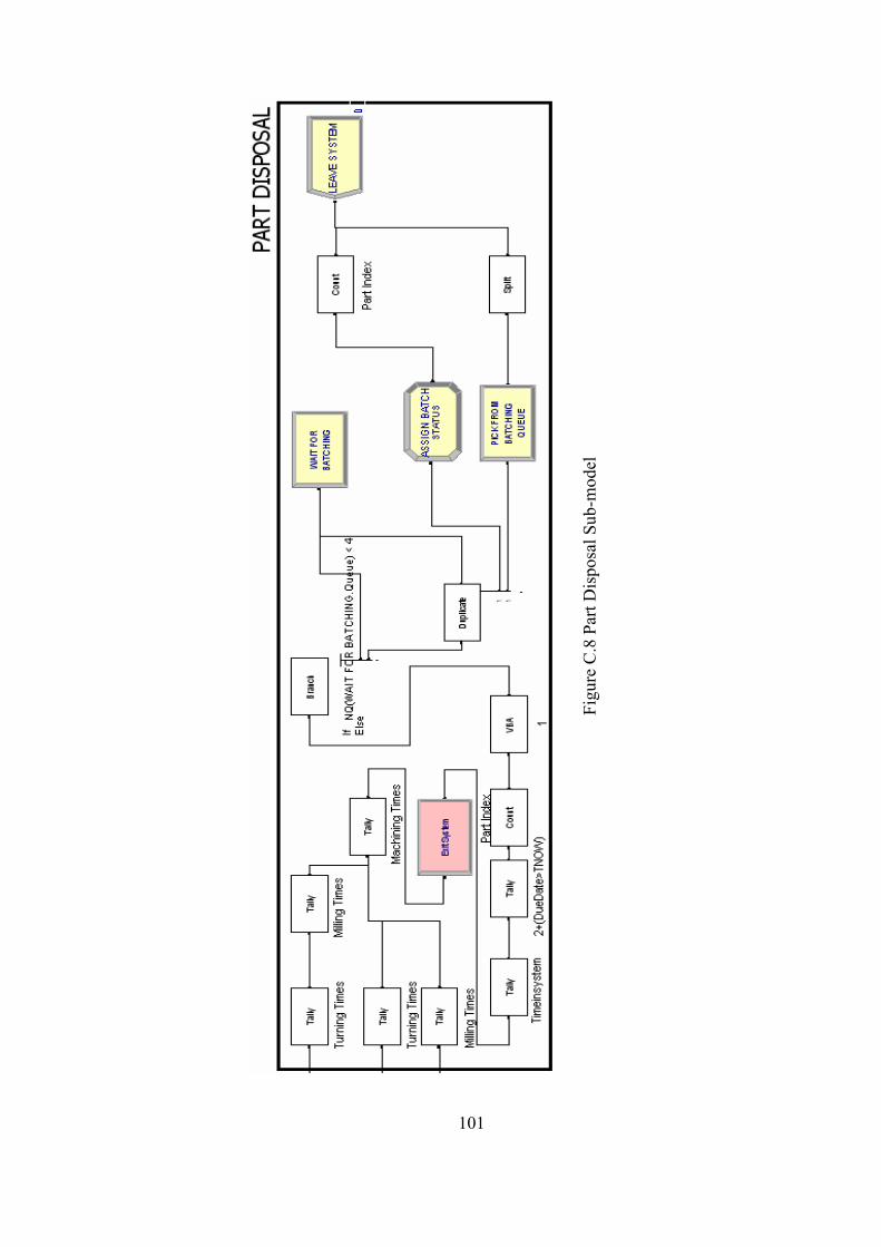
Figu
re C
.8 P
art D
ispo
sal S
ub-m
odel
101

APPENDIX D
D SAMPLE CODE
The following pieces of code are of sample code developed through the realization
of integration of simulation models with external applications. The code and the
associated module are given consecutively.
D.1 Import Data Module:
Private Sub CommandButton1_Click() Dim i, FreeRow, RowValue As Integer
Dim oWorksheet As Excel.Worksheet
FreeRow = 1 i = 0
Sheets("DATA").Select Set oWorksheet = ActiveSheet
With oWorksheet
If .Cells(2, 1) <> 0 Then
Do While i < FreeRow
RowValue = .Cells(i + 2, 1).Value i = i + 1
If RowValue > 0 Then
FreeRow = FreeRow + 1 End If Loop q = "A2: D" & FreeRow Range(q).Select Selection.Delete Shift:=xlUp
102
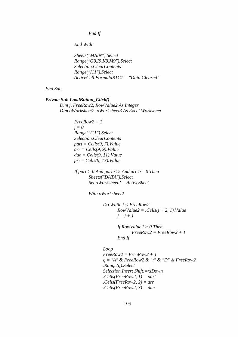
End If
End With
Sheets("MAIN").Select Range("G9,I9,K9,M9").Select Selection.ClearContents Range("I11").Select ActiveCell.FormulaR1C1 = "Data Cleared"
End Sub Private Sub LoadButton_Click()
Dim j, FreeRow2, RowValue2 As Integer Dim oWorksheet2, oWorksheet3 As Excel.Worksheet
FreeRow2 = 1 j = 0 Range("I11").Select Selection.ClearContents part = Cells(9, 7).Value arr = Cells(9, 9).Value due = Cells(9, 11).Value pri = Cells(9, 13).Value
If part > 0 And part < 5 And arr >= 0 Then
Sheets("DATA").Select Set oWorksheet2 = ActiveSheet With oWorksheet2
Do While j < FreeRow2
RowValue2 = .Cells(j + 2, 1).Value j = j + 1 If RowValue2 > 0 Then
FreeRow2 = FreeRow2 + 1 End If
Loop FreeRow2 = FreeRow2 + 1 q = "A" & FreeRow2 & ":" & "D" & FreeRow2 .Range(q).Select Selection.Insert Shift:=xlDown .Cells(FreeRow2, 1) = part .Cells(FreeRow2, 2) = arr .Cells(FreeRow2, 3) = due
103

.Cells(FreeRow2, 4) = pri q = "A1: D" & FreeRow2 q2 = "D" & FreeRow2 .Rows("2:" & FreeRow2).Select Selection.Sort Key1:=Sheets("DATA").Range("B2"), Order1:=xlAscending, Header:=xlNo, OrderCustom:=1, MatchCase:=False, Orientation:=xlTopToBottom, DataOption1:=xlSortNormal
End With
Sheets("MAIN").Select Range("G9,I9,K9,M9").Select Selection.ClearContents Range("I11").Select ActiveCell.FormulaR1C1 = "Data Loaded"
Else
Range("I11").Select ActiveCell.FormulaR1C1 = "Erroneous Data"
End If
End Sub D.2 Export Data Module:
Option Explicit Dim oSIMAN As Arena.SIMAN, nArrivalTimeAttrIndex, nDueDateAttrIndex, nTurnTimeAttrIndex, nMillTimeAttrIndex, nPartTypeIndex, nPriorityIndex, nMaximumConveyor, nConveyorNumber As Long Dim nConveyorTrace(1 To 25) As Long Dim nNextRow As Long, nColumnA, nColumnB, nColumnC, nColumnD, nColumnE, nColumnF, nColumnG, nColumnH, nColumnZ, nColumnY, nColumnP As Long Dim dTurnScheduled, dMillScheduled As Integer Dim nMaxTime As Long Dim oExcelApp As Excel.Application, oWorkbook As Excel.Workbook, oWorksheet, oWorksheet2 As Excel.Worksheet Private Sub ModelLogic_RunBeginReplication() Dim nReplicationNum As Long, i As Integer
104
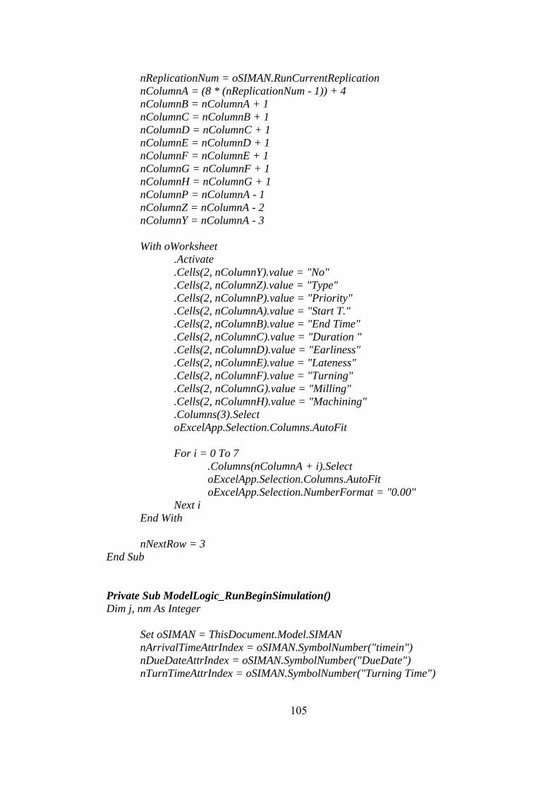
nReplicationNum = oSIMAN.RunCurrentReplication nColumnA = (8 * (nReplicationNum - 1)) + 4 nColumnB = nColumnA + 1 nColumnC = nColumnB + 1 nColumnD = nColumnC + 1 nColumnE = nColumnD + 1 nColumnF = nColumnE + 1 nColumnG = nColumnF + 1 nColumnH = nColumnG + 1 nColumnP = nColumnA - 1 nColumnZ = nColumnA - 2 nColumnY = nColumnA - 3
With oWorksheet
.Activate
.Cells(2, nColumnY).value = "No"
.Cells(2, nColumnZ).value = "Type"
.Cells(2, nColumnP).value = "Priority"
.Cells(2, nColumnA).value = "Start T."
.Cells(2, nColumnB).value = "End Time"
.Cells(2, nColumnC).value = "Duration "
.Cells(2, nColumnD).value = "Earliness"
.Cells(2, nColumnE).value = "Lateness"
.Cells(2, nColumnF).value = "Turning"
.Cells(2, nColumnG).value = "Milling"
.Cells(2, nColumnH).value = "Machining"
.Columns(3).Select oExcelApp.Selection.Columns.AutoFit
For i = 0 To 7
.Columns(nColumnA + i).Select oExcelApp.Selection.Columns.AutoFit oExcelApp.Selection.NumberFormat = "0.00"
Next i End With
nNextRow = 3
End Sub Private Sub ModelLogic_RunBeginSimulation() Dim j, nm As Integer
Set oSIMAN = ThisDocument.Model.SIMAN nArrivalTimeAttrIndex = oSIMAN.SymbolNumber("timein") nDueDateAttrIndex = oSIMAN.SymbolNumber("DueDate") nTurnTimeAttrIndex = oSIMAN.SymbolNumber("Turning Time")
105

nMillTimeAttrIndex = oSIMAN.SymbolNumber("Milling Time") nPartTypeIndex = oSIMAN.SymbolNumber("Part Index") nPriorityIndex = oSIMAN.SymbolNumber("Priority Index") nConveyorNumber = oSIMAN.SymbolNumber("Conveyor 1") nMaximumConveyor = oSIMAN.SymbolNumber("Max Conveyor")
For nm = 1 To 25 nConveyorTrace(nm) = oSIMAN.SymbolNumber("Conveyor Trace", nm, 1) Next nm
Set oExcelApp = CreateObject("Excel.Application") oExcelApp.Visible = False oExcelApp.SheetsInNewWorkbook = 1 Set oWorkbook = oExcelApp.Workbooks.Add Set oWorksheet = oWorkbook.ActiveSheet
'Worksheet 1
With oWorksheet .PageSetup.CenterHeader = "&""Arial,Bold""&16SIMULATION
RESULTS, TALLIES" .PageSetup.LeftMargin = 45 .PageSetup.RightMargin = 45 .Name = "Simulation Results" .Rows(1).Select oExcelApp.Selection.Font.Bold = True oExcelApp.Selection.Font.color = RGB(255, 0, 0) .Rows(2).Select oExcelApp.Selection.Font.Bold = True oExcelApp.Selection.Font.color = RGB(0, 0, 255)
End With 'Worksheet 2
oWorkbook.Sheets.Add Set oWorksheet2 = oWorkbook.ActiveSheet
With oWorksheet2
.PageSetup.CenterHeader = "&""Arial,Bold""&16SIMULATION RESULTS, COUNTERS AND STATISTICS"
.PageSetup.LeftMargin = 45
.PageSetup.RightMargin = 45
.Name = "Statistics"
.Rows(2).Select oExcelApp.Selection.Font.Bold = True oExcelApp.Selection.Font.color = RGB(0, 0, 255)
106

oExcelApp.Selection.Font.Size = 12 .Rows(3).Select oExcelApp.Selection.Font.Bold = True oExcelApp.Selection.Font.color = RGB(255, 0, 0) oExcelApp.Selection.Font.Size = 12 .Rows(10).Select oExcelApp.Selection.Font.Bold = True oExcelApp.Selection.Font.color = RGB(0, 0, 255) oExcelApp.Selection.Font.Size = 12 .Rows(4).Select oExcelApp.Selection.Font.Bold = True .Rows(5).Select oExcelApp.Selection.Font.Bold = True .Rows(6).Select oExcelApp.Selection.Font.Bold = True .Rows(7).Select oExcelApp.Selection.Font.Bold = True .Rows(11).Select oExcelApp.Selection.Font.Bold = True oExcelApp.Selection.Font.color = RGB(255, 0, 0) oExcelApp.Selection.Font.Size = 12 .Rows(12).Select oExcelApp.Selection.Font.Bold = True .Rows(13).Select oExcelApp.Selection.Font.Bold = True .Rows(14).Select oExcelApp.Selection.Font.Bold = True .Rows(15).Select oExcelApp.Selection.Font.Bold = True .Cells(2, 1).value = "PART QUANTITIES BY TYPE" .Cells(3, 1).value = "PART TYPE" .Cells(4, 1).value = "1" .Cells(5, 1).value = "2" .Cells(6, 1).value = "3" .Cells(7, 1).value = "4" .Cells(3, 3).value = "QUANTITY" .Cells(10, 1).value = "FINAL UTILIZATIONS (%)" .Cells(11, 1).value = "RESOURCE NAME" .Cells(12, 1).value = "TURNING" .Cells(13, 1).value = "MILLING" .Cells(14, 1).value = "CONVEYOR" .Cells(15, 1).value = "ROBOT" .Cells(11, 3).value = "VALUE" .Cells(2, 6).value = "SCHEDULED RESOURCES" .Cells(3, 6).value = "RESOURCE NAME" .Cells(3, 8).value = "TIMES" .Cells(4, 6).value = "TURNING"
107

.Cells(5, 6).value = "MILLING"
.Cells(6, 6).value = "ROBOT"
.Cells(10, 6).value = "AVERAGE NUMBER IN QUEUE"
.Cells(11, 6).value = "QUEUE NAME"
.Cells(12, 6).value = "AGV QUEUE" .Cells(11, 8).value = "QUANTITY"
End With End Sub Private Sub ModelLogic_RunEndSimulation() Dim i As Integer
oWorksheet2.Cells(12, 3).value = oSIMAN.DStatAverage(2) * 100 oWorksheet2.Cells(13, 3).value = oSIMAN.DStatAverage(1) * 100 oWorksheet2.Cells(14, 3).value = oSIMAN.DStatAverage(3) * 100 oWorksheet2.Cells(15, 3).value = oSIMAN.DStatAverage(4) * 100 oWorksheet2.Cells(12, 8).value = oSIMAN.DStatAverage(5) oWorksheet2.Columns(2).ColumnWidth = 12.14 oWorksheet2.Columns(7).ColumnWidth = 12.14
With oWorksheet
.Cells(nNextRow, nColumnA).value = "=AVERAGE(R[-" & nNextRow - 3 & "]C:R[-1]C)"
.Cells(nNextRow, nColumnB).value = "=AVERAGE(R[-" & nNextRow - 3 & "]C:R[-1]C)"
.Cells(nNextRow, nColumnC).value = "=AVERAGE(R[-" & nNextRow - 3 & "]C:R[-1]C)"
.Cells(nNextRow, nColumnD).value = "=AVERAGE(R[-" & nNextRow - 3 & "]C:R[-1]C)"
.Cells(nNextRow, nColumnE).value = "=AVERAGE(R[-" & nNextRow - 3 & "]C:R[-1]C)"
.Cells(nNextRow, nColumnF).value = "=AVERAGE(R[-" & nNextRow - 3 & "]C:R[-1]C)"
.Cells(nNextRow, nColumnG).value = "=AVERAGE(R[-" & nNextRow - 3 & "]C:R[-1]C)"
.Cells(nNextRow, nColumnH).value = "=AVERAGE(R[-" & nNextRow - 3 & "]C:R[-1]C)"
.Rows(nNextRow).Select oExcelApp.Selection.Font.Bold = True oExcelApp.Selection.Font.color = RGB(0, 0, 255) .Columns(nColumnZ).Select oExcelApp.Selection.Columns.AutoFit .Columns(nColumnY).Select oExcelApp.Selection.Columns.AutoFit .Cells(nNextRow, nColumnY).value = "AVERAGES"
End With
108

'Time In System Chart
oWorkbook.Sheets("Simulation Results").Select oWorksheet.Range(oWorksheet.Cells(3, nColumnC),
oWorksheet.Cells(nNextRow, nColumnC)).Select oExcelApp.Charts.Add
With oExcelApp.ActiveChart
.ChartType = xlLineMarkers
.SetSourceData Source:=oWorksheet.Range(oWorksheet.Cells(3, nColumnC), oWorksheet.Cells(nNextRow, nColumnC)), PlotBy:=xlColumns .SeriesCollection(1).XValues = "" .Location Where:=xlLocationAsNewSheet, Name:="Time In System" .HasTitle = True .HasAxis(xlValue) = True .HasAxis(xlCategory) = True .HasLegend = False .ChartTitle.Characters.Text = "Time In System" .Axes(xlValue).HasTitle = True .Axes(xlValue).AxisTitle.Characters.Text = "System times in minutes" .Axes(xlCategory).HasTitle = True .Axes(xlCategory).AxisTitle.Characters.Text = "Parts"
End With 'Machining Times Chart
oWorkbook.Sheets("Simulation Results").Select oWorksheet.Range(oWorksheet.Cells(3, nColumnH),
oWorksheet.Cells(nNextRow, nColumnH)).Select oExcelApp.Charts.Add
With oExcelApp.ActiveChart
.ChartType = xlLineMarkers
.SetSourceData Source:=oWorksheet.Range(oWorksheet.Cells(3, nColumnH), oWorksheet.Cells(nNextRow, nColumnH)), PlotBy:=xlColumns .SeriesCollection(1).XValues = "" .Location Where:=xlLocationAsNewSheet, Name:="Machining Times" .HasTitle = True .HasAxis(xlValue) = True .HasAxis(xlCategory) = True .HasLegend = False .ChartTitle.Characters.Text = "Machining Times" .Axes(xlValue).HasTitle = True .Axes(xlValue).AxisTitle.Characters.Text = "Machining times in minutes"
109

.Axes(xlCategory).HasTitle = True
.Axes(xlCategory).AxisTitle.Characters.Text = "Parts" End With
oWorkbook.Sheets("Simulation Results").Select With oExcelApp
.Visible = True
.DisplayAlerts = False End With
' SAVE AS HTML
oWorkbook.SaveAs ThisDocument.Model.Path & "Results2.htm", FileFormat:=xlHtml, ReadOnlyRecommended:=False, CreateBackup:=False oWorkbook.SaveAs ThisDocument.Model.Path & "Results.xls"
End Sub D.3 VBA Modules:
Private Sub VBA_Block_1_Fire() Dim dCreateTime As Double, dCurrentTime As Double Dim dDueDate, dTurnTime, dMillTime As Double Dim dPartIndex, dPriorityIndex As Integer
dCreateTime = oSIMAN.EntityAttribute(oSIMAN.ActiveEntity, nArrivalTimeAttrIndex) dCurrentTime = oSIMAN.RunCurrentTime dDueDate = oSIMAN.EntityAttribute(oSIMAN.ActiveEntity, nDueDateAttrIndex) dTurnTime = oSIMAN.EntityAttribute(oSIMAN.ActiveEntity, nTurnTimeAttrIndex) dMillTime = oSIMAN.EntityAttribute(oSIMAN.ActiveEntity, nMillTimeAttrIndex) dPartIndex = oSIMAN.EntityAttribute(oSIMAN.ActiveEntity, nPartTypeIndex) dPriorityIndex = oSIMAN.EntityAttribute(oSIMAN.ActiveEntity, nPriorityIndex)
‘ assign part no create time current time and time in system
With oWorksheet .Cells(nNextRow, nColumnY).value = nNextRow - 2 .Cells(nNextRow, nColumnA).value = dCreateTime
110

.Cells(nNextRow, nColumnB).value = dCurrentTime
.Cells(nNextRow, nColumnC).value = dCurrentTime - dCreateTime
.Cells(nNextRow, nColumnH).value = dMillTime + dTurnTime
.Cells(nNextRow, nColumnZ).value = dPartIndex
.Cells(nNextRow, nColumnP).value = dPriorityIndex
If dPartIndex = 1 Then .Cells(nNextRow, nColumnZ).Interior.color = RGB(255, 255,
0) ElseIf dPartIndex = 2 Then
.Cells(nNextRow, nColumnZ).Interior.color = RGB(128, 128, 0) ElseIf dPartIndex = 3 Then
.Cells(nNextRow, nColumnZ).Interior.color = RGB(128, 0, 0) Else
.Cells(nNextRow, nColumnZ).Interior.color = RGB(255, 0, 0) End If
End With ' assign earliness and lateness
If (dDueDate >= dCurrentTime) Then oWorksheet.Cells(nNextRow, nColumnD).value = dDueDate -
dCurrentTime Else
oWorksheet.Cells(nNextRow, nColumnE).value = dCurrentTime - dDueDate End If
' assign Turning and Milling times If dTurnTime > 0 Then oWorksheet.Cells(nNextRow, nColumnF).value =
dTurnTime If dMillTime > 0 Then oWorksheet.Cells(nNextRow, nColumnG).value =
dMillTime If (dCurrentTime - dCreateTime) > nMaxTime Then nMaxTime =
(dCurrentTime - dCreateTime)
nNextRow = nNextRow + 1 oWorksheet2.Cells(6, 8).value = oSIMAN.CounterValue(8) oWorksheet2.Cells(4, 3).value = oSIMAN.CounterValue(1) oWorksheet2.Cells(5, 3).value = oSIMAN.CounterValue(2) oWorksheet2.Cells(6, 3).value = oSIMAN.CounterValue(3) oWorksheet2.Cells(7, 3).value = oSIMAN.CounterValue(4)
End Sub Private Sub VBA_Block_2_Fire() oWorksheet2.Cells(4, 8).value = oSIMAN.CounterValue(6)
111

End Sub Private Sub VBA_Block_3_Fire() oWorksheet2.Cells(5, 8).value = oSIMAN.CounterValue(7) End Sub D.4 Interface Module
Private Sub ModelLogic_RunBegin() frmArrivalTypeSelection.Show End Sub Private Sub cmdOK_Click() Dim nCreateRandomProcessIndex As Long Dim oCreateRandomProcessModule As Arena.Module Dim nCreateFileIndex As Long Dim oCreateFileModule As Arena.Module Dim oModel As Arena.Model Dim nSoundfileIndex As Long
Set oModel = ThisDocument.Model nCreateRandomProcessIndex = oModel.Modules.Find(smFindTag, "Create
from random process") If nCreateRandomProcessIndex = 0 Then
MsgBox "No Module with tag 'Create from random process'" frmArrivalTypeSelection.Hide Exit Sub
End If Set oCreateRandomProcessModule = oModel.Modules(nCreateRandomProcessIndex) nCreateFileIndex = oModel.Modules.Find(smFindTag, "Create from file")
If nCreateFileIndex = 0 Then
MsgBox "No Module with tag 'Create from file'" frmArrivalTypeSelection.Hide Exit Sub
End If Set oCreateFileModule = oModel.Modules(nCreateFileIndex)
112

If optFromRandomProcess.value = False Then
oCreateRandomProcessModule.Data("Max Batches") = "0" oCreateFileModule.Data("Max Batches") = "1"
Else oCreateFileModule.Data("Max Batches") = "0" oCreateRandomProcessModule.Data("Max Batches") = "180"
End If frmArrivalTypeSelection.Hide Exit Sub End Sub
113

APPENDIX E
E PART PROCESS PLANS
The layout of METUCIM system was described in detail in Chapter 3. According to
this layout, a part can have four possible process plans assuming that all operations
of one single type (milling or turning) can be finished in one pass. The parts can
have only one milling / turning operation or milling can follow turning or vice versa.
Part variability can be obtained by assigning different processing times for
operations in the machines. The representation of entities that belong to the
mentioned types is based on coloring in the simulation. Each type is shown with a
different color and parts take the color of the type that they belong to. The types,
associated colors and assigned machining sequences are given on Table E.1
Table E.1 Part types, process sequences and durations
PART TYPE TURNING MILLING COLOR
1 2 / TRIA (2.4, 2.5, 2.6) 1 / TRIA (1.4, 1.5, 1.6) YELLOW
2 - 1 / TRIA (2.8, 3.0, 3.2) BRONZE
3 1 / TRIA (7.2, 7.5, 7.8) - RUBY
4 1 / TRIA (9.6, 10, 10.4) 2 / TRIA (5.6, 6, 6.4) RED
In addition to coloring the parts, the completed level of the process plan can be
followed on the parts. Each part that has finished its task on one of the machines
takes a letter over its representing picture (M for Milling and T for Turning), which
114

shows the completed tasks on the part. A part that has completed both of the
operations has both T and M letters on it.
115

APPENDIX F
F FLOWCHART
The basic flowchart of events for the developed models is given on Figure F.1.
Figure F.1 Basic Flowchart of events for the models.
116