Simulation Modelling Practice and Theory 69 (2016) 80–91

Contents lists available at ScienceDirect

Simulation Modelling Practice and Theory

journal homepage: www.elsevier.com/locate/simpat

A simulation analysis of part launching and order collection

decisions for a flexible manufacturing system

Yi-Chi Wang

a , ∗, Toly Chen

a , Hsiangtsai Chiang

b , Hui-Chen Pan

a

a Department of Industrial Engineering and Systems Management, Feng Chia University, No. 100, Wenhwa Rd., Seatwen, Taichung 40724,

Taiwanb Department of Accounting, Feng Chia University, No. 100, Wenhwa Rd., Seatwen, Taichung 40724, Taiwan

a r t i c l e i n f o

Article history:

Received 18 July 2015

Revised 24 May 2016

Accepted 19 September 2016

Keywords:

Simulation

Part launching

Order collection

Flexible manufacturing system

a b s t r a c t

In a dynamic flexible manufacturing system (FMS) environment jobs arrive randomly, and

in most of the existing studies the due date for a single part is set individually. However,

when the due date is set for an order that consists of multiple parts, some completed

parts may have to wait for the rest of the order to be completed. This paper studied the

scheduling problem in the FMS in which orders require the completion of different parts

in various quantities. The orders arrive randomly and continuously, and all have prede-

termined due dates. Two scheduling decisions were considered in this study: launching

parts into the system for production, and determining the order sequence for collecting

the completed parts. A new part-launching rule, named the Tardiness Estimating Method

(TEM) was proposed. A discrete-event simulation model of the FMS was developed and

used as a test-bed for experiments under various system conditions. The proposed part

launch rule was capable of providing good performance regarding minimum mean tardi-

ness and maximum service level, but provided only a moderate flow time when compared

with the other five rules commonly used in the literature. In addition, three order collec-

tion rules were tested in the experiments. Collecting parts for the order with the earliest

due date (EDD) was found better than the other rules for tardiness related measures.

© 2016 Published by Elsevier B.V.

1. Introduction

Given the increased level of global competition, the common challenge is that every modern manufacturing enterprise

must be capable of making customized high-quality products with small lot sizes and short lead times in order to survive

in today’s competitive market. A flexible manufacturing system (FMS) is a computerized and highly automated production

system that is designed to produce a mid-volume and a mid-variety of products at a high level of efficiency. This type of

production system combines the efficiency of a mass production line with the flexibility of a job shop and is the best fit

for modern manufacturing enterprises to boost their productivity and competitiveness [1] . Since the successful implemen-

tation of the first flexible manufacturing system (FMS) in the 1960s, an abundance of FMS issues have been studied. A FMS

usually consists of a set of computer numerically controlled machines (CNCs) linked with an automated material handling

system. One of the characteristics distinguishing the FMS from other manufacturing systems is that the FMS provides routing

∗ Corresponding author. Fax: + 886 4 24510240.

E-mail addresses: wangyc@fcu.edu.tw , wang_yichi@yahoo.com.tw (Y.-C. Wang).

http://dx.doi.org/10.1016/j.simpat.2016.09.006

1569-190X/© 2016 Published by Elsevier B.V.

Y.-C. Wang et al. / Simulation Modelling Practice and Theory 69 (2016) 80–91 81

flexibility because of the capability of modern CNC machines, essentially allowing the design of alternative process plans for

a job. This flexibility and level of automation make the FMS an extremely complex, large-scale modern production system.

A large amount of research has been conducted to solve problems such as loading, scheduling, automated guided vehicle

(AGV) dispatching, or cutting tools management in FMSs. Most of the existing literature treats a job as a single order when

released into the FMS, and each job in the shop normally represents a single type of part. The problem investigated in this

study is that an order may require to complete different parts, each part in different quantities. Contrary to launching a part

with a production due date, this problem involves two decisions as follows:

(1) Part launch: this refers to the selection of the parts to be loaded onto a pallet with at the loading/unloading end of

the FMS for subsequent processing in the system.

(2) Order collection: since there may be many different parts that must be completed in the output buffer of FMS, they

must be collected to form a completed order for shipment. This decision refers to deciding the order of collecting the

completed parts and the subsequent shipment.

The purpose of this paper is to provide a simulation analysis by examining the above two decisions when operating

a dynamic FMS. A discrete-event simulation model for a make-to-order FMS was developed and used as a test-bed for

experiments under various system conditions. The remainder of this paper is organized as follows. Section 2 reviews the

literature on scheduling as well as FMS control issues. Section 3 details the FMS simulation model used in the present

research. Section 4 describes the order collection rules and the part launch rules as well as the experimental conditions in

this study. Section 5 discusses the simulation results. Finally, in Section 6 conclusions are drawn and directions for future

research are provided.

2. Literature review

A large amount of literature has been devoted on the examination of the effects of the planning and scheduling strategies

of the FMS, both from an operational and a control point of view. To implement a FMS, the following issues must be taken

into consideration [2] :

• Sequencing of the parts to be loaded into the system. • Part routing. • Sequence the parts waiting in each machine to be processed. • Sequence those parts that require transportation. • Allocate material handling devices to fulfill the transportation requirements of the parts.

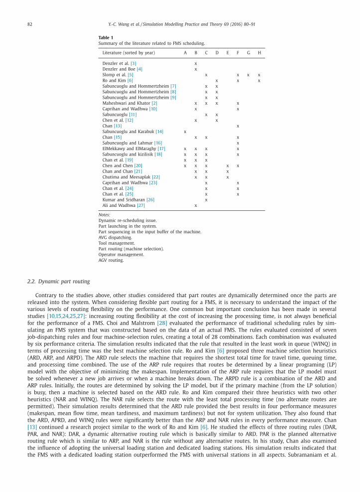
These five issues can be further classified into eight scheduling problems. Table 1 provides a summary of the literature

focusing on these eight problems. It is obvious that the top three are part launching (B), part routing (F), and part sequencing

in the machine buffer (C).

2.1. Fixed part routing

In some studies, the part routes were determined in the FMS planning phase. In these studies the focus was on schedul-

ing problems other than the dynamic part routing problem. For example, Sabuncuoglu and Hommertzheim [7] examined

the effects of the dispatching rules used for prioritizing the jobs waiting for processing in the machine queue, and the

rules to dispatch an automated guided vehicle (AGV) under various experimental conditions. They found that the smallest

modified operation due-date (MOD) was the best rule for sequencing the jobs in the machine queue, and that the largest

queue size (LQS) was the preferred rule for the dispatching an AGV for various due-date criteria. For different criteria, like

minimizing the mean flow time, these researchers indicated that the shortest processing time (SPT) combined with any AGV

rule tended to be suitable [8] . Among the AGV rules examined, LQS and STD (shortest travel distance) in combination with

any machine rule proved to be the best rules. These authors also investigated the performance of the rules under various

approaches of setting the internal due dates in a FMS [9] . They found that the ‘flow-allowance is proportional to the total

work’ (TWK) rule outperformed other due-date setting rules by minimizing the mean tardiness for most of the conditions

tested. Sabuncuoglu [11] extended their earlier work to measure the sensitivity of the machine and the AGV scheduling rules

to the processing time distributions, loading levels, and machine and AGV breakdowns. The results of their study showed

that the performance of scheduling rules is affected by the variances of the distribution of the operating time, the different

system loading levels, as well as the machine downtime percentage.

Sabuncuoglu and Lahmar [16] compared two operation grouping policies: aggregation and disaggregation. In the aggre-

gation case, all the operations required for making a part are performed at a single machine. The machine does not release

a part until all the operations required are completed. Disaggregation is the process of assigning the operations required on

a part to various machines. In short, aggregation is the case of a single-stage multi-machine FMS [26] , while disaggregation

is the case of a normal FMS. Their study concluded that although FMS managers may advocate the aggregation approach in

order to reduce the number of setups, the aggregation approach is not always advantageous in a variety of FMS environ-

ments. They also concluded that the disaggregation approach is only suitable for FMSs composed of non-identical machines,

and especially under heavy loading conditions.

82 Y.-C. Wang et al. / Simulation Modelling Practice and Theory 69 (2016) 80–91

Table 1

Summary of the literature related to FMS scheduling.

Literature (sorted by year) A B C D E F G H

Denzler et al. [3] x

Denzler and Boe [4] x

Slomp et al. [5] x x x x

Ro and Kim [6] x x x

Sabuncuoglu and Hommertzheim [7] x x

Sabuncuoglu and Hommertzheim [8] x x

Sabuncuoglu and Hommertzheim [9] x x

Maheshwari and Khator [2] x x x x

Caprihan and Wadhwa [10] x x

Sabuncuoglu [11] x x

Chen et al. [12] x x

Chan [13] x

Sabuncuoglu and Karabuk [14] x

Chan [15] x x x

Sabuncuoglu and Lahmar [16] x

ElMekkawy and ElMaraghy [17] x x x x

Sabuncuoglu and kizilisik [18] x x x x

Chan et al. [19] x x x

Chen and Chen [20] x x x x x

Chan and Chan [21] x x x

Chutima and Meesaplak [22] x x x

Caprihan and Wadhwa [23] x x

Chan et al. [24] x x

Chan et al. [25] x x

Kumar and Sridharan [26] x

Ali and Wadhwa [27] x

Notes:

Dynamic re-scheduling issue.

Part launching in the system.

Part sequencing in the input buffer of the machine.

AVG dispatching.

Tool management.

Part routing (machine selection).

Operator management.

AGV routing.

2.2. Dynamic part routing

Contrary to the studies above, other studies considered that part routes are dynamically determined once the parts are

released into the system. When considering flexible part routing for a FMS, it is necessary to understand the impact of the

various levels of routing flexibility on the performance. One common but important conclusion has been made in several

studies [10,15,24,25,27] : increasing routing flexibility at the cost of increasing the processing time, is not always beneficial

for the performance of a FMS. Choi and Malstrom [28] evaluated the performance of traditional scheduling rules by sim-

ulating an FMS system that was constructed based on the data of an actual FMS. The rules evaluated consisted of seven

job-dispatching rules and four machine-selection rules, creating a total of 28 combinations. Each combination was evaluated

by six performance criteria. The simulation results indicated that the rule that resulted in the least work in queue (WINQ) in

terms of processing time was the best machine selection rule. Ro and Kim [6] proposed three machine selection heuristics

(ARD, ARP, and ARPD). The ARD rule selects the machine that requires the shortest total time for travel time, queuing time,

and processing time combined. The use of the ARP rule requires that routes be determined by a linear programing (LP)

model with the objective of minimizing the makespan. Implementation of the ARP rule requires that the LP model must

be solved whenever a new job arrives or when a machine breaks down. The ARPD rule is a combination of the ARD and

ARP rules. Initially, the routes are determined by solving the LP model, but if the primary machine (from the LP solution)

is busy, then a machine is selected based on the ARD rule. Ro and Kim compared their three heuristics with two other

heuristics (NAR and WINQ). The NAR rule selects the route with the least total processing time (no alternate routes are

permitted). Their simulation results determined that the ARD rule provided the best results in four performance measures

(makespan, mean flow time, mean tardiness, and maximum tardiness) but not for system utilization. They also found that

the ARD, APRD, and WINQ rules were significantly better than the ARP and NAR rules in every performance measure. Chan

[13] continued a research project similar to the work of Ro and Kim [6] . He studied the effects of three routing rules (DAR,

PAR, and NAR): DAR, a dynamic alternative routing rule which is basically similar to ARD. PAR is the planned alternative

routing rule which is similar to ARP, and NAR is the rule without any alternative routes. In his study, Chan also examined

the influence of adopting the universal loading station and dedicated loading stations. His simulation results indicated that

the FMS with a dedicated loading station outperformed the FMS with universal stations in all aspects. Subramaniam et al.

Y.-C. Wang et al. / Simulation Modelling Practice and Theory 69 (2016) 80–91 83

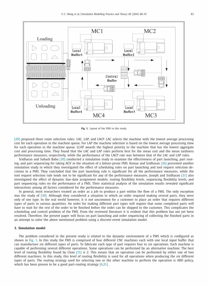
Fig. 1. Layout of the FMS in this study.

[29] proposed three route selection rules: LAC, LAP, and LACP. LAC selects the machine with the lowest average processing

cost for each operation in the machine queue. For LAP the machine selection is based on the lowest average processing time

for each operation in the machine queue. LCAP awards the highest priority to the machine that has the lowest aggregate

cost and processing time. They found that the LAC and LAP rules perform best for the mean cost and the mean tardiness

performance measures, respectively, while the performance of the LACP rule was between that of the LAC and LAP rules.

Sridharan and Subash Babu [30] conducted a simulation study to examine the effectiveness of part launching, part rout-

ing, and part sequencing for taking AGV in the situation of a failure-prone FMS. Kumar and Sridharan [26] presented another

simulation study in which they investigated the effect of scheduling rules on part launching and tool request selection de-

cisions in a FMS. They concluded that the part launching rule is significant for all the performance measures, while the

tool request selection rule tends not to be significant for any of the performance measures. Joseph and Sridharan [31] also

investigated the effect of dynamic due-date assignment models, routing flexibility levels, sequencing flexibility levels, and

part sequencing rules on the performance of a FMS. Their statistical analysis of the simulation results revealed significant

interactions among all factors considered for the performance measures.

In general, most researchers treated an order as a job to produce a part within the flow of a FMS. The only exception

was the study of [30] . Although they considered a situation in which an order required making several parts, they were

only of one type. In the real world however, it is not uncommon for a customer to place an order that requires different

types of parts in various quantities. An order for making different part types will require that some completed parts will

have to wait for the rest of the order to be finished before the order can be shipped to the customer. This complicates the

scheduling and control problem of the FMS. From the reviewed literature it is evident that this problem has not yet been

resolved. Therefore, the present paper will focus on part launching and order sequencing of collecting the finished parts in

an attempt to solve the above mentioned problem using a discrete-event simulation model.

3. Simulation model

The problem considered in the present study is related to the dynamic environment of a FMS which is configured as

shown in Fig. 1 . In this study the FMS is comprised of four different CNC machines each with one local input buffer that

can manufacture six different types of parts. To fabricate each type of part requires four to six operations. Each machine is

capable of performing several different operations. Some operations can be performed by an alternative machine. The best

level of routing flexibility found by Chan [15] is 2. This means that an operation can be performed by either one of two

different machines. In this study, this level of routing flexibility is used for all operations when producing the six different

types of parts. The routing strategy used for selecting one or the other machine to perform the operation is ARD policy,

which has been proven to be a good part-routing strategy [6,21] .

84 Y.-C. Wang et al. / Simulation Modelling Practice and Theory 69 (2016) 80–91

Table 2

Process plan for part types/processing times and required fixtures

(unit: minutes).

Part type Operation Machine Fixture type

1 2 3 4

A 1 7 3 — — 3

2 — 11 — 1 3

3 — 6 6 — 1

4 1 — — 7 2

B 1 5 — 10 — 1

2 — — 9 2 2

3 — 8 — 4 2

4 8 — 7 — 3

5 5 — — 9 2

6 — — 7 11 1

C 1 6 — 8 — 1

2 — — 4 7 2

3 8 — — 4 3

4 6 10 — — 1

5 — 9 — 7 2

D 1 — — 7 8 3

2 9 8 — — 1

3 — 1 3 — 2

4 10 — 9 — 2

5 — 7 — 8 1

E 1 3 — 5 — 1

2 — 1 — 10 3

3 10 — — 8 1

4 — 2 7 — 2

5 4 6 — — 2

6 — — 7 2 1

F 1 2 — 6 — 3

2 7 — — 5 3

3 — 4 2 — 1

4 — — 5 11 2

Chan and Chan [21] conducted a comprehensive survey on scheduling issues of the FMS. They found that most of re-

searchers focused on only a few decision points. Modeling a complex FMS with multiple decisions points may be difficult,

but it is necessary to make the model as close as possible to reality. They also pointed out that some authors considered

only time-processing-based rules and ignored due-date based rules. From the summary they provided, it is evident that only

a scant few authors consider more than one scheduling problem like part dispatching problems, machine selection prob-

lems, and AGV scheduling problems simultaneously in their simulation models. Raj et al. [1] reviewed some implementation

issues of the FMS and pointed out that there is a wide gap between research on the FMS and the actual implementation

of a FMS. They addressed the importance of including the issues of AGV dispatching, the machining tools and equipment

management. Thus, in our simulation model, the AGV transportation time, the pallets and the dedicated fixtures for the

parts are all taken into consideration.

When a particular operation of a part is completed by a machine, that part will then be sent to the central buffer and

stays there until it is transported to another machine for its next operation. If a fixture replacement is necessary, the part

will be sent to the loading area and re-enter the system after the proper fixture for the next operation is successfully

installed. All transportation is handled by four AGVs. The transportation times are calculated based on the distance between

the facilities involved (shown in Table 2 ) and the AGV’s travelling speed. When a part requires transportation, only the AGVs

that are free at that time are taken into consideration. If there is more than one AGV free at the same time, then the request

will be sent to the AGV closest to where the part is. This is the STD rule which is suggested from the study of Sabuncuoglu

and Hommertzheim [8] . Each AGV may receive several requests from parts. It may be worth trying various AGV dispatching

rules like MOD, LQS, et cetera. Since AGV dispatching is not our focus in this study, FCFS (first come first served) is employed

in the transportation request selection for an AGV.

In this study the simulated FMS is developed on the following assumptions:

• Each machine can carry out only one operation at a time. • A part in the loading area is available for launching into the system when a pallet and a proper fixture are available. • Operation preemption is not allowed. • Processing times for each operation are deterministic. All the processing times are presented in Table 3. • The part may revisit the same machine before completing all its manufacturing steps. • Machines may break down. The mean time between failures is set at 34,200 min and the mean time for repairing the

broken machine is set at 18 min.

Y.-C. Wang et al. / Simulation Modelling Practice and Theory 69 (2016) 80–91 85

Table 3

Distances between the facilities (unit: meter).

To/From L/UL MC1 MC2 MC3 MC4 WIP

L/UL — 12.15 18 36 41.85 24.3

MC1 41.85 — 5.85 23.85 29.7 12.15

MC2 36 41.85 — 18 23.85 21.15

MC3 18 30.15 36 — 5.85 12.15

MC4 12.15 24.3 30.15 48.15 — 21.15

WIP 9 21.15 27 12.15 21.15 —

Table 4

Notation used in this study.

SCT Simulation Clock Time.

P k The estimated processing time per piece for operation k . This value is determined by averaging two of the

processing times performed by two different machines.

ETPT i The estimated total processing time for order i . This is computed by summing all the estimated processing

times for the required operations.

IC j Inter-completion time of the last two completed parts (for part type j ).

IQ j The quantity of part type j that has been launched for production.

Q j The required quantity of part type j .

ETM j The estimated total processing time for all the remaining quantity of part type j .

ET j The estimated tardiness for part type j .

D Due date for a certain order.

• All pallets are general-purpose pallets. The capacity of each pallet is one part and the total number of pallets is limited

to fifteen. • Dedicated fixtures are used for each operation (i.e. an operation can only be performed using a dedicated fixture). The

number of each fixture type is limited to ten. • Parts may return to the input buffer of the system if changing to a proper fixture is required. • A part must leave the system and vacate its pallet and the fixture when all their operations are finished. • Local buffer capacity for each machine is limited and is set at 5. • No collisions occur along the AGV path. • There is no scrap produced by the machines. • Once the order is placed, no cancelation is allowed.

4. Operational and control strategies in the FMS

The most difficult part of the present problem is that each order requires making different parts in various quantities.

Making a part requires the completion of a series of operations. In the FMS model, each operation can be performed with

one of two machines and the system is capable of making 6 different types of parts. Once several orders have arrived it is

time for the production launch. Logically, the decision in which order the production will be launched should be determined

before sequencing the part for launching into the system. However, the manufacturing lead time for the different parts

varies based on processing time, resource (machines/AGVs) availability, equipment (pallet/fixture) usage, and levels of part

congestion in the system. This also makes it difficult to control the production of different part types in different quantities.

In that case, the sequence for part launching is based on the output of the FMS. In other words, we first determine the order

for the complete part collection. With this information we then decide which part type should be launched for production.

4.1. Order collection rules

As mentioned above, the first decision that must be made is determining for which order to collect the completed parts.

The notations used in this paper are presented in Table 4 . The three scheduling rules employed in the present study are

described as follows.

• Early Due Date (EDD): Collect the completed parts for the order with the earliest due date. • Critical Ratio (CR): The critical ratio (CR i ) for order i is defined as follows:

C R i = ( D i − SCT ) /ET P T i (1)

With this rule, the highest priority is given to the order with the smallest CR value.

• Minimum Slack Time (MST): The remaining slack in order i , defined as ( D i − ETPT i – SCT ), is computed. The order with

the minimum remaining slack time will be selected for completed part collection.

86 Y.-C. Wang et al. / Simulation Modelling Practice and Theory 69 (2016) 80–91

With any of these three order collection rules, order pre-emption is allowable in this study. In other words, the operators

may be forced to change the order they use for collecting the completed parts. When this happens, those parts that have

been collected will be used for the new order.

4.2. Part launching rules

A part launch rule is used to select the next part type for a production launch in the FMS. The proposed part launch rule

as well as the other 5 rules commonly used in the literature is described as follows:

• TEM (Tardiness Estimation Method): The proposed part launch rule is designed to estimate tardiness ( ET j ) for each part

type and to choose the part type with the largest estimated tardiness value for the production launch. The value of ET j is computed as follows.

E T j = ( SCT + ET M j ) − D (2)

Where ET M j = ( Q j − I Q j ) × I C j (3)

• LRPQ (Largest Remaining Production Quantity): The part type with the largest remaining production work is assigned

the highest priority for the next production launch. • LRPQ/TPQ (Largest Ratio of Remaining Production Quantity over Total Production Quantity): The part type with the

largest remaining production quantity over the total production quantity is assigned the highest priority for the next

production cycle. • LTRW (Longest Total Remaining Production Work): The part type with the largest remaining production work is assigned

the highest priority for the next production cycle. Production work refers to the total processing time for making the

quantity of parts ordered. • LRUW/TRPQ (Smallest Ratio of Unit Production Work over Total Remaining Production Quantity): The part type with the

smallest ratio of the unit production work divided by the remaining production quantity. • RANDOM: Randomly select one of six types of parts.

4.3. Performance measures

Four performance measures are used for evaluation as follows:

• Mean tardiness: Tardiness is the positive difference between the completion time of an order and its due date. • Maximum tardiness: This measure is important because customers may tolerate a small amount of tardiness but may be

very upset for larger ones. • Service rate: The ratio of the number of no-tardy orders to the total number of orders completed. • Mean flow time: The average time orders spend in the FMS; from launching the first part for production to the last part

being completed.

5. Experimental results

The simulation model was developed using the discrete-event simulation technique. It was programed in C ++ language

and was implemented on a personal computer. The elements in the FMS such as machines, orders, parts, and AGVs, are all

developed using objects. With such modulized elements (objects), this simulation model can easily be extended to as many

stages (machining processes) and many elements in the stage of the FMS as needed. This simulation model logically mimics

the interactions within the elements of the FMS and can be used to see how the output performance measures are affected

by exercising numerically the model for the inputs. The model was verified and validated by the techniques recommended

by Law and Kelton [32] . The model may also be constructed with the multi-agent distributed modeling technique [33] . A

horizon of 10,0 0 0 order completions was determined to be an appropriate run length under all conditions to guarantee that

the system had reached a steady state. After these 10,0 0 0 orders were completed as a system warm-up, 50 0 0 additional

orders were processed for computing the performance measures. In this study, two phases of simulation analysis were

conducted. In Phase I, we adopted EDD as the only rule for completed parts collection, and compared the six part launching

rules described earlier under four different system conditions. These four system conditions were set by varying the mean

inter-arrival time of the orders in the system and the tightness of the due date. The time between the orders arriving in the

system follows an exponential distribution, with a mean of 800 min representing a heavy loading condition and 900 min a

light loading condition. The due date of the order was determined based on the following equation:

Due date = Arrival time + Allowance factor ( K ) ×Estimated total processing time

The allowance factor was drawn from the uniform distribution between 0.65 and 1.45, U (0.65, 1.45), for orders with tight

due dates and between 1.65 and 2.45, U (1.65, 2.45), for orders with loose due dates. The settings are shown in Table 5 .

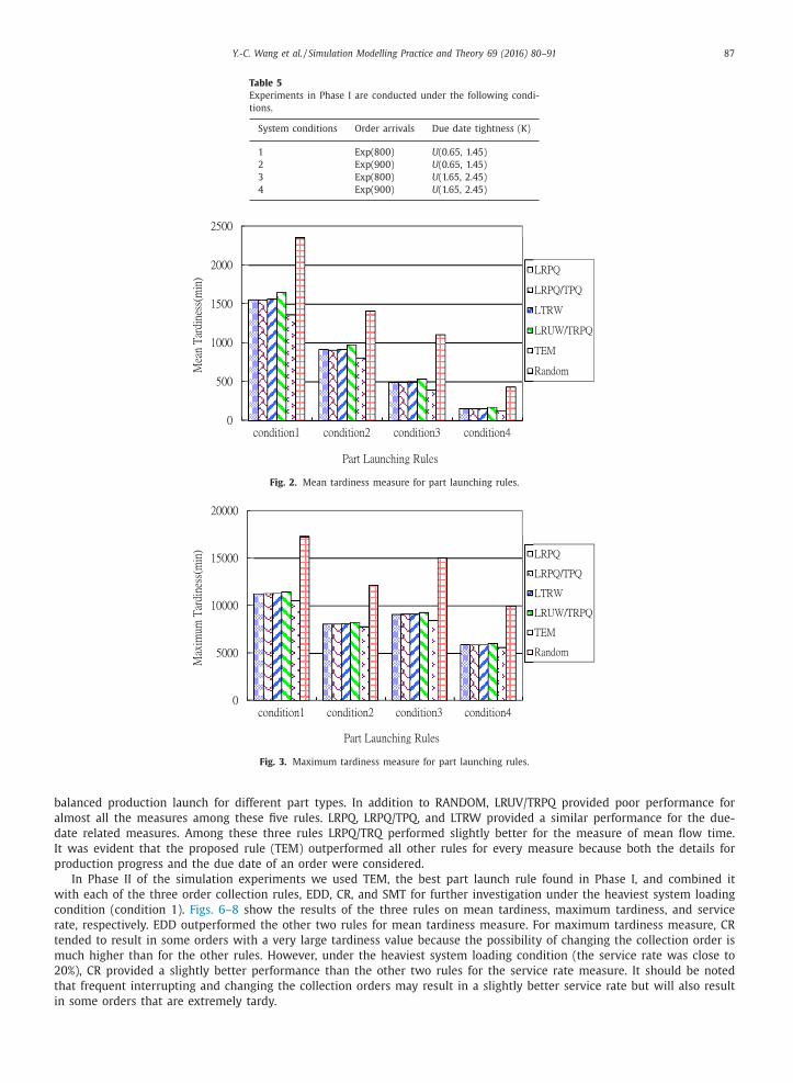
Figs. 2 –5 show the simulation results for the mean tardiness, maximum tardiness, service rate, and mean flow time

measures, respectively. Randomly selecting a part type for the production launch proved to be a bad idea for the three due

date related measures compared with the other five rules. It however did give a shorter mean flow time because of the

Y.-C. Wang et al. / Simulation Modelling Practice and Theory 69 (2016) 80–91 87

Table 5

Experiments in Phase I are conducted under the following condi-

tions.

System conditions Order arrivals Due date tightness (K)

1 Exp(800) U (0.65, 1.45)

2 Exp(900) U (0.65, 1.45)

3 Exp(800) U (1.65, 2.45)

4 Exp(900) U (1.65, 2.45)

Fig. 2. Mean tardiness measure for part launching rules.

Fig. 3. Maximum tardiness measure for part launching rules.

balanced production launch for different part types. In addition to RANDOM, LRUV/TRPQ provided poor performance for

almost all the measures among these five rules. LRPQ, LRPQ/TPQ, and LTRW provided a similar performance for the due-

date related measures. Among these three rules LRPQ/TRQ performed slightly better for the measure of mean flow time.

It was evident that the proposed rule (TEM) outperformed all other rules for every measure because both the details for

production progress and the due date of an order were considered.

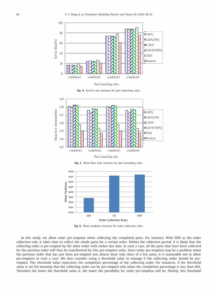
In Phase II of the simulation experiments we used TEM, the best part launch rule found in Phase I, and combined it

with each of the three order collection rules, EDD, CR, and SMT for further investigation under the heaviest system loading

condition (condition 1). Figs. 6 –8 show the results of the three rules on mean tardiness, maximum tardiness, and service

rate, respectively. EDD outperformed the other two rules for mean tardiness measure. For maximum tardiness measure, CR

tended to result in some orders with a very large tardiness value because the possibility of changing the collection order is

much higher than for the other rules. However, under the heaviest system loading condition (the service rate was close to

20%), CR provided a slightly better performance than the other two rules for the service rate measure. It should be noted

that frequent interrupting and changing the collection orders may result in a slightly better service rate but will also result

in some orders that are extremely tardy.

88 Y.-C. Wang et al. / Simulation Modelling Practice and Theory 69 (2016) 80–91

Fig. 4. Service rate measure for part launching rules.

Fig. 5. Mean flow time measure for part launching rules.

Fig. 6. Mean tardiness measure for order collection rules.

In this study, we allow order pre-emption when collecting the completed parts. For instance, With EDD as the order

collection rule, it takes time to collect the whole parts for a certain order. Within the collection period, it is likely that the

collecting order is pre-empted by the other order with earlier due date. In such a case, all the parts that have been collected

for the previous order will then be transformed for this pre-emptive order. Since order pre-emption may be a problem when

the previous order that has just been pre-empted was almost done only short of a few parts, it is reasonable not to allow

pre-emption in such a case. We thus consider using a threshold value to manage if the collecting order should be pre-

empted. This threshold value represents the completion percentage of the collecting order. For instances, if the threshold

value is set 0.6 meaning that the collecting order can be pre-empted only when the completion percentage is less than 60%.

Therefore the lower the threshold value is, the lower the possibility for order pre-emption will be. Shortly, this threshold

Y.-C. Wang et al. / Simulation Modelling Practice and Theory 69 (2016) 80–91 89

Fig. 7. Maximum tardiness measure for order collection rules.

Fig. 8. Service rate measure for order collection rules.

Fig. 9. Mean tardiness measure of using various threshold values to manage order preemption.

value determines how much likely order pre-emption may occur. In order to evaluate how this threshold value may affect

those performance measures. We test the system only under the system condition 1. Under this condition, the due date

allowance factor is determined according to U (0.65, 1.45). Such high variations for the due date allowance factor will cause

more order pre-emption if the threshold value is also set high. Figs. 9 and 10 show how different levels of the threshold

value for managing order pre-emption affect the performance measures on mean tardiness and service level, respectively.

In Fig. 9 , it is evident that setting the threshold value 0.8 offers the best performance on mean tardiness measure. While, In

Fig. 10 , the lower the threshold value is, the higher the service level can be reached.

90 Y.-C. Wang et al. / Simulation Modelling Practice and Theory 69 (2016) 80–91

Fig. 10. Service level measure of using various threshold values to manage order preemption.

6. Conclusions

This paper presented a simulation study that was conducted to analyze the part launch and order collection decisions

in the FMS. All the decisions were examined in the two phases of the experiments. The part launch rules considered for

experimentation included LRPQ, LQPQ/TPQ, LTRW, LRUW/TRPW, and the proposed TEM in addition to the RANDOM rule. The

simulation results in Phase I of the experiments revealed that the proposed TEM rule outperformed the other rules in all the

performance measures. Three order collection rules, EDD, CR, and MST were tested under a heavy loading system condition.

EDD outperformed the others for almost all the measures. The significance of frequently changing the order (pre-emption)

of the part collection was addressed in the simulation analysis in Phase II of the experiments.

Acknowledgments

This study was financially supported by the National Science Council of Taiwan under Contract no. NSC 100-2221-E-035-

076-MY3 .

References

[1] T. Raj , R. Shankar , M. Suhaib , A review of some issues and identifications of some barriers in the implementation of FMS, Int. J. Flex. Manuf. Syst. 19

(2007) 1–14 . [2] S.K. Maheshwari , S.K. Khator , Simultaneous evaluation and selection of strategies for loading and controlling machines and material handling system

in FMS, Int. J Comput. Integr. Manuf. 8 (1995) 340–356 . [3] D.R. Denzler , W.J. Boe , D. Edward , An experimental investigation of FMS scheduling rules under uncertainty, J. Oper. Manag. 7 (1987) 139–151 .

[4] D.R. Denzler , W.J. Boe , Experimental investigation of flexible manufacturing system scheduling decision rules, Int. J. Prod. Res. 25 (1987) 979–994 .

[5] J. Slomp , G.J.C. Gaalman , W.M. Nawijn , Quasi on-line scheduling procedures for flexible manufacturing systems, Int. J. Prod. Res. 26 (1988) 585–598 . [6] I.-K. Ro , J.I. Kim , Multi-criteria operational control rules in flexible manufacturing systems (FMSs), Int. J. Prod. Res. 28 (1990) 47–63 .

[7] I. Sabuncuoglu , D.L. Hommertzheim , Experimental investigation of FMS machine and AGV scheduling rules against the mean flow-time criterion, Int.J. Prod. Res. 30 (1992) 1617–1635 .

[8] I. Sabuncuoglu , D.L. Hommertzheim , Experimental investigation of an FMS due-date scheduling problem: Evaluation of machine and AGV schedulingrules, Int. J. Flex. Manuf. Syst. 5 (1993) 301–323 .

[9] I. Sabuncuoglu , D.L. Hommertzheim , Experimental investigation of an FMS due-date scheduling problem: An evaluation of due-date assignment rules,

Int. J. Comput. Integr. Manuf. 8 (1995) 133–144 . [10] R. Caprihan , S. Wadhwa , Impact of routing flexibility on the performance of an FMS – A simulation study, Int. J. Flex. Manuf. Syst. 9 (1997) 273–298 .

[11] I. Sabuncuoglu , A study of scheduling rules of flexible manufacturing systems: A simulation approach, Int. J. Prod. Res. 36 (1998) 527–546 . [12] F.F. Chen , J. Huang , M.A. Centeno , Intelligent scheduling and control of rail-guided vehicles and load/unload operations in a flexible manufacturing

system, J. Intell. Manuf. 10 (1999) 405–421 . [13] F.T.S. Chan , Evaluations of operational control rules in scheduling a flexible manufacturing system, Robot. Comput. Integr. Manuf. 15 (1999) 121–132 .

[14] I. Sabuncuoglu , S. Karabuk , Rescheduling frequency in an FMS with uncertain processing times and unreliable machine, J. Manuf. Syst. 18 (1999)

268–283 . [15] F.T.S. Chan , The effects of routing flexibility on a flexible manufacturing system, Int. J. Comput. Integr. Manuf. 14 (2001) 431–445 .

[16] I. Sabuncuoglu , M. Lahmar , An evaluative study of operation grouping policies in an FMS, Int. J. Flex. Manuf. Syst. 15 (2003) 217–239 . [17] T.Y. ElMekkawy , H.A. ElMaraghy , Real-time scheduling with deadlock avoidance in flexible manufacturing systems, Int. J. Adv. Manuf. Technol. 22

(2003) 259–270 . [18] I. Sabuncuoglu , O.B. Kizilisik , Reactive scheduling in a dynamic and stochastic FMS environment, Int. J. Prod. Res. 41 (2003) 4211–4231 .

[19] F.T.S. Chan , H.K. Chan , H.C.W. Lau , R.W.L. Ip , Analysis of dynamic dispatching rules for a flexible manufacturing system, J. Mater. Process. Technol. 138

(2003) 325–331 . [20] J. Chen , F.F. Chen , Adaptive scheduling in random flexible manufacturing systems subject to machine breakdowns, Int. J. Prod. Res. 41 (2003)

1927–1951 . [21] F.T.S. Chan , H.K. Chan , Analysis of dynamic control strategies of an FMS under different scenarios, Robot. Comput. Integr. Manuf. 20 (2004) 423–437 .

[22] P. Chutima , C. Meesaplak , Operational control decisions in FMS under expediting conditions, Thammasat Int. J. Sci. Technol. 9 (2004) 37–46 . [23] R. Caprihan , S. Wadhwa , Scheduling of FMSs with information delays: A simulation study, Int. J. Flex. Manuf. Syst. 17 (2005) 39–65 .

Y.-C. Wang et al. / Simulation Modelling Practice and Theory 69 (2016) 80–91 91

[24] F.T.S. Chan , R. Bhagwat , S. Wadhaw , Increase in flexibility: Productivity or counterproductivity? A study on the physical and operating characteristicsof a flexible manufacturing system, Int. J. Prod. Res. 44 (2006) 1431–1445 .

[25] F.T.S. Chan , R. Bhagwat , S. Wadhwa , Flexibility performance: Taguchi’s method study of physical system and operating control parameters of FMS,Robot. Comput. Integr. Manuf. 23 (2007) 25–37 .

[26] N.S. Kumar , R. Sridharan , Simulation modeling and analysis of part and tool flow control decisions in a flexible manufacturing system, Robot. Comput.Integr. Manuf. 25 (2009) 829–838 .

[27] M. Ali , S. Wadhwa , The effect of routing flexibility on a flexible system of integrated manufacturing, Int. J. Prod. Res. 48 (2010) 5691–5709 .

[28] R.H. Choi , E.M. Malstrom , Evaluation of traditional work scheduling rules in a flexible manufacturing system with a physical simulator, J. Manuf. Syst.7 (1988) 33–45 .

[29] V. Subramaniam , G.K. Lee , T. Ramesh , G.S. Hong , Y.S. Wong , Machine selection rules in a dynamic jog shop, Int. J. Adv. Manuf. Technol. 16 (20 0 0)902–908 .

[30] R. Sridharan , A. Subash Babu , Multi-level scheduling decisions in a class of FMS using simulation based metamodels, J. Oper. Soc. 49 (1998) 591–602 .[31] O.A. Joseph , R. Sridharan , Analysis of dynamic due-date assignment models in a flexible manufacturing system, J. Manuf. Syst. 30 (2011) 28–40 .

[32] A.M. Law , W.D. Kelton , Simulation Modeling and Analysis, McGraw Hill, 20 0 0 . [33] F. Cicirelli , A. Furfaro , L. Nigro , Modelling and simulation of complex manufacturing systems using statechart-based actors, Simul. Model. Pract. Theory

19 (2011) 685–703 .