www.elsevier.com/locate/foreco

Forest Ecology and Management 214 (2005) 65–90

Simulation and quantification of the fine-scale spatial pattern and

heterogeneity of forest canopy structure: A lacunarity-based

method designed for analysis of continuous canopy heights

Gordon W. Frazer a,*, Michael A. Wulder b, K. Olaf Niemann a

a Department of Geography, University of Victoria, P.O. Box 3050, STN CSC, Victoria, BC, Canada V8W 3P5b Canadian Forest Service, Pacific Forestry Centre, 506 West Burnside Road, Victoria, BC, Canada V8Z 1M5

Received 21 January 2005; received in revised form 12 March 2005; accepted 16 March 2005

Abstract

Forests canopies are dynamic, continuously varying, three-dimensional structures that display substantial heterogeneity in

their spatial arrangement at many scales. At the stand-level, fine-scale spatial heterogeneity influences key canopy processes and

contributes to the diversity of niche space and maintenance of forest biodiversity. We present a quantitative method that we

developed based on a novel application of two well-established statistical techniques – lacunarity analysis and principal

component analysis (PCA) – to determine the fine-scale (0.5–33 m) spatial heterogeneity found in the outer surface of a forest

canopy. This method was specifically designed for the analysis of continuous canopy height data generated by airborne LiDAR

systems or digital photogrammetry; however, in this study we demonstrate our method using a large, well-documented dataset

composed of simulated canopy surfaces only. We found that the magnitude of the lacunarity statistic was strongly associated

with canopy cover (R2 = 0.85) and gap volume (R2 = 0.84), while the pattern of decline in lacunarity across discrete

measurement scales was related to many size- and density-related attributes of stand and canopy structure

(0.27 � R2 � 0.58) and their diverse vertical and horizontal spatial distributions. PCA uncovered two major gradients of

spatial heterogeneity from the 10 dimensions of our original lacunarity dataset. The stronger of these two gradients reflected the

continuous variation in canopy cover and gap volume, while a second, more subtle gradient was associated with the array of

possible vertical and horizontal spatial configurations that might define any one measure of canopy cover. We expect that this

quantitative method can be used to support a broad range of practical applications in sustainable forest management, long-term

ecological monitoring, and forest science. Further research is required to understand how these statistical estimates and gradients

of measured spatial heterogeneity relate to other ecologically relevant patterns of forest composition, structure, and function.

# 2005 Elsevier B.V. All rights reserved.

Keywords: Canopy height models; Canopy structure; Forest structure; Lacunarity analysis; Laser remote sensing; LiDAR; Principal

component analysis; Spatial heterogeneity; Spatial pattern analysis

* Corresponding author. Tel.: +1 250 656 4852; fax: +1 250 721 6216.

E-mail addresses: gfrazer@uvic.ca (G.W. Frazer), mwulder@pfc.forestry.ca (M.A. Wulder), oniemann@office.geog.uvic.ca

(K.O. Niemann).

0378-1127/$ – see front matter # 2005 Elsevier B.V. All rights reserved.

doi:10.1016/j.foreco.2005.03.056

G.W. Frazer et al. / Forest Ecology and Management 214 (2005) 65–9066

Nomenclature

BA basal area (m2) per hectare (ha)

CC canopy cover (%)

CD quadratic mean crown diameter (m)

CHM canopy height model

CW quadratic mean crown width (m)

DBH diameter at breast height (cm)

GAP gap volume (%)

HL Lorey’s mean stand height (m)

LiDAR light detection and ranging

PC1 first principal component

PC2 second principal component

PCA principal component analysis

PO modified Pollard’s nearest-neighbour

statistic

QMD quadratic mean diameter (cm)

r box size of gliding window (grid-cell

units)

RD Curtis’ relative density

s box size of gliding window (m)

SD stand density (n/ha)

SHDI Shannon’s Height Diversity Index

VOL stand volume (m3/ha)

L(r) lacunarity statistic measured at box size

r

LTOTAL normalized lacunarity statistic inte-

grated across all scales r

1. Introduction

Heterogeneity is an inherent, ubiquitous, and

critical property of ecological systems, and is thought

to sustain many aspects of ecosystem function and

biodiversity across space and through time (Kolasa

and Pickett, 1991; Caldwell and Pearcy, 1994; Pickett

et al., 1997). Heterogeneity, as an ecological concept

and system property, has many definitions, occurs in

many forms (Kolasa and Rollo, 1991), and is strongly

dependent on the spatiotemporal scales of observation

and methods of measurement (Legendre and Fortin,

1989; Gardner, 1998; Gustafson, 1998; Dale, 1999).

Forest ecosystems are often described by attributes of

composition, structure, and function (Franklin et al.,

2002), and heterogeneity arises when any or all of

these attributes vary in space, time, or both (Dutilleul

and Legendre, 1993; Li and Reynolds, 1995; Franklin

and Van Pelt, 2004).

A precise definition of spatial heterogeneity

depends upon the nature of the ecological pattern

and entities of interest (Dutilleul and Legendre, 1993;

Gustafson, 1998). For example, discontinuous spatial

phenomena (e.g., individual tree locations, nest sites,

etc.) form distinctive point patterns that are a result of

their distribution throughout a region of space (Dale,

1999). In this case, spatial heterogeneity is defined by

variability in density of the discrete objects or entities

(referred to as events in point pattern literature) in

space, and by their degree of departure from

complete spatial randomness (CSR) towards aggre-

gation or overdispersion (regularity or uniformity).

CSR occurs when discrete events are dispersed both

randomly and independently of one another (Diggle,

2003). Many ecological processes and system

attributes, on the other hand, occur more continu-

ously over space or time (e.g., photosynthesis,

temperature, humidity, canopy density, etc.). Con-

tinuous spatial phenomena are considered to be

heterogeneous when one or more ecosystem attri-

butes vary across discrete subregions of space in an

irregular or non-random manner (Dutilleul and

Legendre, 1993). Measures of spatial heterogeneity

are almost always tied to variability in time, because

ecosystems are by definition inherently dynamic in

both space and time (Gustafson, 1998).

Forest canopies are dynamic, continuously varying,

three-dimensional (3-D) spatial structures composed

mostly of leaves, twigs, branches, and the open spaces

(gaps) among them (Parker, 1995). Canopies are

shaped by all components of stand structure including

live tree-size and age distributions, stem density,

species composition, crown widths and depths, leaf

area and density, growth form, and the spatial

arrangement of individual boles (Spies, 1998). The

fine-scale spatial structure of forest canopies is often

conceptualized within a hierarchical framework

(Fournier et al., 1997), where individual leaves are

organized into increasingly coarser-scale structures,

such as shoots or twigs, branches, whorls, crowns, and

finally into spatial neighbourhoods of individual

crowns (Parker, 1995; Song et al., 1997; Cescatti,

1998). At coarser spatial scales, discrete neighbour-

G.W. Frazer et al. / Forest Ecology and Management 214 (2005) 65–90 67

1 Second-order stationarity exists when an attribute of interest is

normally distributed with the same mean and variance over the

entire sampling area (Legendre and Legendre, 1998). Under con-

ditions of second-order stationarity, covariance between a pair of

random variables is only dependent on the distance of separation

between sample points and not on location within the study area.

Spatial stationarity is often an unreasonable assumption for hetero-

geneous forest canopies because of continuously varying local and

regional influences of resource and environmental heterogeneity,

community composition, successional processes, and disturbance

regimes on all aspects of stand and canopy structure.

hoods of individual crowns coalesce to form homo-

geneous stands (patches), which may be similar in

disturbance history, age class, species composition,

and site productivity, and between-patch rather than

within-patch spatial heterogeneity emerges as the

dominant characteristic of forest structure (Lertzman

and Fall, 1998).

Fine-scale canopy structure and its vertical and

horizontal spatial heterogeneity play key roles in

regulating the spatial and temporal variability of stand

microclimate (Chen et al., 1999), light interception,

photosynthesis, carbon gain, and primary production

(Parker, 1995), atmosphere–biosphere exchanges of

energy, matter, and trace gases (Parker et al., 2004a),

nutrient and hydrological cycles (Prescott, 2002;

Nadkarni and Sumera, 2004), stand dynamics (Can-

ham et al., 1994; Herwitz et al., 2000), and

biodiversity (Carey, 2003; Ishii et al., 2004; Spies,

2004). Fine-scale canopy patterns, processes, and

dynamics naturally scale across larger aggregates of

time and space, and therefore also contribute to

broader-scale ecological patterns, processes, and

dynamics (Ehleringer and Field, 1993; Saunders

et al., 1998).

Despite the significance of spatial heterogeneity in

theoretical and applied ecology, few methods exist to

determine this key attribute of forest canopy structure.

Quantification of spatial heterogeneity has been

hampered in the past by four main factors. First,

consensus on an operational definition of spatial

heterogeneity did not exist in ecology until recently

(Kolasa and Rollo, 1991; Dutilleul and Legendre,

1993; Li and Reynolds, 1995). Second, those relying

on analytical techniques that measure spatial pattern

or texture at only one, arbitrarily defined, observation

scale have ignored the fact that pattern is often highly

scale-dependent (Gardner, 1998; Dale, 1999). Third,

limited access to the forest canopy has forced many

researchers to rely on ground-based sampling, datasets

of restricted dimensionality (i.e., points and transects),

and aspatial metrics (e.g., Shannon’s Index; Staud-

hammer and LeMay, 2001) to characterize the spatial

heterogeneity associated with 3-D patterns of canopy

structure. Last, many of the statistical techniques (e.g.,

semivariance, Moran’s I, Geary’s c, and Grey Level

Co-occurrence Matrix) commonly used to quantify

spatial pattern in ecological or remotely sensed data

depend, in varying degrees, on the unlikely assump-

tion of second-order stationarity1 to remain unbiased

(Henebry and Kux, 1995; Weishampel et al., 2001;

Perry et al., 2002).

Efforts to quantify the spatial heterogeneity of

forest canopies have focused on three distinct

methodological approaches. The first approach relies

on skyward-looking, ground-based optical instru-

ments such as solar radiation sensors (Baldocchi

and Collineau, 1994; Brown and Parker, 1994;

Montgomery and Chazdon, 2001), fisheye photogra-

phy (Walter and Himmler, 1996; Trichon et al., 1998;

Frazer et al., 2000), and range-finding lasers (Parker

et al., 2004b) to characterize canopy structure.

Aspatial statistical descriptions of these field data

include mean values of key canopy variables (e.g., gap

fraction, openness, leaf area index) and their variances

(Trichon et al., 1998; Frazer et al., 2000), and diversity

indices describing vertical distributions of canopy

elements (Parker et al., 2004b). The scale-dependent

structure of sunflecks, gaps, leaf area, and canopy

height over a given spatial domain has been

investigated using semivariance, spectral analysis,

wavelets, and local quadrat variances (Bradshaw and

Spies, 1992; Baldocchi and Collineau, 1994; Walter

and Himmler, 1996; Bartemucci et al., 2002).

The second methodological approach utilizes the

simulated or real point pattern of tree locations

coupled with 3-D crown models or spatial tessellations

(e.g., Zenner and Hibbs, 2000) to explore the

continuously varying structure of forest canopies

(Van Pelt and North, 1996; Song et al., 1997; Chen and

Bradshaw, 1999; Van Pelt and Franklin, 2000;

Silbernagel and Moeur, 2001; Song et al., 2004;

Van Pelt and Nadkarni, 2004). In forest research,

nearest-neighbour and Ripley’s K statistical analyses

are commonly used to determine if a pattern of

discrete events (stem locations) or points between the

G.W. Frazer et al. / Forest Ecology and Management 214 (2005) 65–9068

events are spatially random, aggregated, or over-

dispersed (Moeur, 1993; Stoyan and Penttinen, 2000).

Ripley’s K was specifically designed to identify the

scale dependence of these point patterns. In addition,

vertical and hemispherical projections of canopy

crown models (Van Pelt and North, 1996; Song et al.,

1997; Silbernagel and Moeur, 2001) and the size

distribution of patches (polygons) generated by spatial

tessellation (Zenner and Hibbs, 2000) have facilitated

the measurement of canopy patchiness in the

horizontal domain. Sampling 3-D canopy models in

the vertical dimension has been used to determine the

spatial variability of intercrown gaps and crown

volume from the top of forest canopy to the forest floor

(Van Pelt and North, 1996; Song et al., 2004).

Finally, the fine-scale spatial pattern and structure

of forest canopies have been studied from above

using air- and spaceborne optical (Cohen et al.,

1990; Treitz and Howarth, 2000), radar (Sun and

Ranson, 1998), and laser (light detection and

ranging, LiDAR) remote sensing (Drake and

Weishampel, 2000; Weishampel et al., 2000; Ollier

et al., 2003; Parker and Russ, 2004). Small-footprint,

discrete-return LiDAR has been identified as a

particularly useful remote sensing technology in

forest studies (Lefsky et al., 2002; Lim et al., 2003),

because of its unique ability to accurately measure

fine-scale (<1 m) canopy structure in both vertical

and horizontal spatial domains (Zimble et al., 2003;

Koukoulas and Blackburn, 2004; Parker et al.,

2004a; Parker and Russ, 2004).

The main purpose of this paper is to describe a

quantitative method that we devised for measuring the

fine-scale (<50 m) spatial heterogeneity or texture

found in the surface topography of a forest canopy.

This technique is based on a novel application of two

well-established statistical techniques: lacunarity

analysis and principal component analysis. We used

the lacunarity statistic as a scale-dependent estimate of

canopy texture and spatial non-stationarity, while PCA

facilitated the separation of individual sample units

along unique gradients of spatial pattern and canopy

structure based on differences in lacunarity measured

at nine discrete spatial scales. Our method was

designed specifically for the analysis of two-dimen-

sional (2-D) canopy height models extracted from

airborne LiDAR data; however, in this study we

demonstrate its application using simulated canopy

surfaces only. We have five principal objectives in this

paper:

(1) T

o provide a brief introduction to lacunarity as a

concept and analytical method, and to describe its

potential application to 2-D quantitative canopy

height data.

(2) T

o present a detailed case study illustrating the

scale-dependent response of the lacunarity statis-

tic to five different simulated canopy surface

patterns.

(3) T

o demonstrate how lacunarity analysis and PCA

can be combined to effectively separate a large

number of canopy surface patterns in reduced

ordination space based on cross-scale differences

in spatial heterogeneity.

(4) T

o identify specific attributes of canopy structure

that contributed to the unique spatial and

structural gradients uncovered by lacunarity

analysis and PCA.

(5) T

o suggest a number of potential ecological

applications for this research.

2. Spatial pattern analysis

2.1. Lacunarity as a scale-dependent measure of

spatial heterogeneity in forest canopies

Lacunarity derives from the Latin word, lacuna,

meaning ‘gap’, and was first introduced by Mandel-

brot (1983, p. 310) to describe the ‘gapiness’ or texture

of fractals. The concept of lacunarity, however, applies

equally to non-fractals (Allain and Cloitre, 1991), and

is more formally defined as the scale-dependent

deviation of a geometrical object or pattern from

translational invariance or homogeneity (Geffen et al.,

1983; Cheng, 1997). Geometrical patterns with low

lacunarity are finely textured and homogeneous

with respect to the size distribution and spatial

arrangement of gaps. In contrast, coarsely textured

patterns that show substantial heterogeneity in the size

distribution and spatial arrangement of gaps are

described as being highly ‘lacunar’ (Blumenfeld and

Mandelbrot, 1997). Statistical estimates of lacunarity

are strongly dependent on both the spatial scale (i.e.,

grain or resolution) and extent of observation

(Plotnick et al., 1993; Dale, 2000). For example, a

G.W. Frazer et al. / Forest Ecology and Management 214 (2005) 65–90 69

spatial pattern that is heterogeneous at one observation

scale may appear homogeneous at finer or coarser

measurement scales. Similarly, one region of space

may reveal a very different scale-dependent pattern of

heterogeneity than another region. Lacunarity has

therefore become a useful concept and analytical

technique to study the scale-dependent heterogeneity

of a broad range of spatiotemporal phenomena in

ecology and remote sensing (e.g., Plotnick et al., 1996;

Sun and Ranson, 1998; Weishampel et al., 2000;

Saunders et al., 2005).

The spatial pattern and structure of the outer surface

of a forest canopy is determined by the size, shape,

abundance, and spatial distribution of canopy trees (or

overstory), as well as by the varied gap sizes found

within and among tree crowns. Spatial heterogeneity in

the height of the outer canopy surface can be observed at

many different scales. For example, leaf display, branch

geometry, and within-crown gaps contribute to the finest

scales of canopy height variation. At coarser spatial

scales, heterogeneity is created by differences in the size

and geometry of individual crowns and intercrown gaps.

Finally, local variations in stem density, species

composition, and spatial aggregation among crowns

of similar size and height (patches of regeneration,

biological legacies, or dominant canopy trees), and

major tree-fall gaps produce the coarsest scales of stand-

level spatial heterogeneity in forest canopy height.

We created two separate sets of simulated

50 m � 50 m (0.25 ha) forest canopy height models

(CHM) to demonstrate how lacunarity analysis can be

used to examine the cross-scale spatial pattern and

heterogeneity of forest canopies. The first simulated

dataset included 5 CHMs, while the second consisted of

187 separate CHMs. The size of each of these datasets

was arbitrarily chosen. We utilized the first dataset to

briefly illustrate and explain the scale-dependent

response of the lacunarity statistic to a few simple

and complex canopy surface patterns. We then used the

larger, second dataset to show how lacunarity analysis

and PCA facilitated the separation and comparison of

sample units in reduced ordination space based on

cross-scale differences in canopy surface pattern. We

chose a 3-D simulation approach rather than LiDAR-

generated CHMs to develop this quantitative method,

because simulation permitted us strict control over the

composition and spatial arrangement of stand structure,

and it also allowed us to quickly generate a large, well-

documented dataset covering a broad range of canopy

surface patterns. Nevertheless, we recognize that

simulated CHMs lack the fine-scale detail (i.e., foliage

and branch architecture, and within-crown gaps) and

coarse-scale realism of natural forest patterns (i.e.,

dispersion of tree locations), as well as the measurement

error or noise inherent in all remotely sensed data.

However, our intent here was not to derive an ecological

interpretation of these simulated data, but rather only to

illustrate and explain the statistical behaviour of

lacunarity as a potentially useful quantitative measure

of spatial heterogeneity in forest canopy research.

2.2. Lacunarity analysis using the ‘gliding-box’

algorithm and 2-D quantitative data

The ‘gliding-box’ algorithm (see Plotnick et al.,

1993, 1996 for description) was first introduced by

Allain and Cloitre (1991) to compute the lacunarity of

random or deterministic fractal sets composed of binary

(i.e., occupied (M = 1) or unoccupied (M = 0)) patterns.

However, the method was later expanded to include

scale-dependent measures of lacunarity for fractal and

non-fractal sets (binary patterns) and fields (quantita-

tive spatial data) of one or more Euclidean dimensions

(Plotnick et al., 1996; Cheng, 1997; Kirkpatrick and

Weishampel, in press). Here, we use the gliding-

box algorithm to compute lacunarity at discrete

measurement scales s (0.5 � s � 33 m) by sampling

the distribution of mass across a regularized m

(columns) � n (rows) grid of quantitative canopy

heights xij. In this application, mass M (box mass) is

defined as the sum or integral of all canopy heights xkl

contained within a square gliding box of linear size r,

where r is the box size measured in grid-cell units (i.e.,

r = 1, 2, 3, . . .), and subscripts k and l are unique column

and row identifiers for each cell height xij summed

within the bounds of the gliding box. The frequency

distribution of mass at box size r is sampled by gliding a

box of size r one grid-cell position at a time starting at

the origin of the grid until all columns i and rows j of the

m � n grid have been sampled. The total number of

boxes N(r) of size r required to cover the entire m � n

grid is given by Sun and Ranson (1998):

NðrÞ ¼ ðm � r þ 1Þðn � r þ 1Þ (1)

The frequency distribution of mass M at box size r

is converted to a probability function Q(M, r) by

G.W. Frazer et al. / Forest Ecology and Management 214 (2005) 65–9070

dividing the frequency of each mass M by N(r) (Allain

and Cloitre, 1991). The first and second statistical

moments of the probability function Q(M, r) are

estimated using the following equations (Cheng, 1997;

Dale, 2000):

Zð1ÞQ ðrÞ ¼ 1

NðrÞXm�rþ1

i¼1

Xn�rþ1

j¼1

Xiþr�1

k¼1

Xjþr�1

l¼1

xkl (2)

Xm�rþ1 Xn�rþ1 Xiþr�1 Xjþr�1 !2

Zð2ÞQ ðrÞ ¼ 1

NðrÞi¼1 j¼1 k¼1 l¼1

xkl (3)

Finally, lacunarity at box size r is computed as a

dimensionless statistic using the equation:

LðrÞ ¼Zð2ÞQ ðrÞ

½Zð1ÞQ ðrÞ2

¼ 1 þs2

QðrÞ½Zð1Þ

Q ðrÞ2(4)

where s2QðrÞ is the sample variance and Z

ð1ÞQ ðrÞ is the

mean of the probability function Q(M, r) (Plotnick

et al., 1996; Cheng, 1997). Repeating the lacunarity

calculations at box sizes ranging from r = 1 to some

proportion of the shortest length of the grid map

reveals a unique scale-dependent pattern of decline

in the logarithm of the lacunarity statistic when plotted

against the logarithm of box size.

2.3. Five examples illustrating the application of

lacunarity analysis to forest CHMs

Canopy surface patterns have been simulated by

others using a combination of spatial point processes

and 3-D crown modeling techniques (e.g., Song et al.,

2004; Van Pelt and Nadkarni, 2004). Three of the five

simulated CHMs presented here are examples of

random, aggregated, and uniform (overdispersed)

point patterns each composed of 100 trees (Fig. 1;

Table 1). The first three examples (Fig. 1A–C) are

represented by different point patterns with identical

tree heights and crown dimensions, while the last two

examples (Fig. 1D and E) have the same random

pattern as Fig. 1A, but with variable tree heights and

crown sizes. In the last example (Fig. 1E), the stand

table used to generate Fig. 1D was spatially sorted so

that tree height increased with decreasing distance

along the X dimension of the plot.

Lacunarity analyses of these five CHMs produce

very distinct curves when logarithmic transforms of

lacunarity L(r) and box size r are plotted against one

another (Fig. 2). All double-log curves show a decline

in lacunarity with increase in box size; however, all

curves differ in magnitude at their maxima, some

decline more rapidly than others (e.g., A, C, F), and all

show subtle breaks in slope at different measurement

scales. Self-similar fractals produce lacunarity curves

that are straight lines, with slopes equal to fractal

dimension D minus Euclidean dimension E (Allain

and Cloitre, 1991; Plotnick et al., 1996). Lacunarity is

determined by the proportion of the grid map covered

by vegetative canopy, and by the mean and variance of

the distribution of canopy heights across the plot

(Feagin, 2003). Dividing each value of lacunarity L(r)

by L(1) eliminates the effect of the first statistical

moment (mean), thereby normalizing the lacunarity

curve to a common Y-intercept of 1 (Plotnick et al.,

1996; Feagin, 2003). Normalization of the lacunarity

statistic L(r) allows direct comparison of curves

between sample plots of different canopy height,

cover, and spatial pattern (bottom graph, Fig. 2).

Three general characteristics of the lacunarity

statistic L(r) emerge from analysis of these five CHMs

and through other published studies (e.g., Plotnick

et al., 1996; Dale, 2000). First, lacunarity at box size

r = 1 will increase as the percentage of canopy cover

decreases and gap volume increases. For example,

Model B (Fig. 1B) has the highest lacunarity

(L(1) = 3.669), lowest canopy cover (32.9%), and

highest gap volume (77.6%) of all five models, while

Model D (Fig. 1D) has the lowest lacunarity

(L(1) = 1.733), highest canopy cover (68.5%), and

lowest gap volume (37.7%). In general, larger values

of the lacunarity statistic observed at a given spatial

scale imply greater spatial heterogeneity, texture, or

‘patchiness’ of the canopy surface at that scale. On the

other hand, lacunarity values approaching 1 indicate

low spatial variability in canopy heights and therefore

greater translational invariance or homogeneity in the

canopy surface at that scale of measurement.

Second, the rate of decline in lacunarity with

increasing box size depends on the presence and

heterogeneity of coarser-scale patterns. Lacunarity

curves that decline more slowly with increasing spatial

scale indicate the occurrence of coarser-scale patterns

(Plotnick et al., 1993, 1996). Alternatively, lacunarity

curves showing a rapid decline with increasing box

size imply spatial randomness or uniformity at coarser

G.W. Frazer et al. / Forest Ecology and Management 214 (2005) 65–90 71

Fig. 1. Five examples of simulated 3-D stand models (top graphic) and canopy height models (middle and bottom graphics) developed for: (A)

random, (B) aggregated, and (C) uniform distributions of tree locations. We used the stem locations generated for the random model to create two

other more complex canopy patterns by (D) randomly assigning a range of tree sizes to the random stem locations and (E) by spatially sorting

these variable tree sizes so that tree height increased with decreasing distance along the X-axis of the plot. All five canopy height models contain

the same number of trees (n = 100), and have a spatial-resolution of 0.5 m.

G.W. Frazer et al. / Forest Ecology and Management 214 (2005) 65–9072

Fig. 1. (Continued )

G.W. Frazer et al. / Forest Ecology and Management 214 (2005) 65–90 73

Fig. 1. (Continued ).

measurement scales. Dale (2000) suggests using

randomization procedures (see Manly, 1997) and

CSR as the null model if tests of statistical significance

are required. Lacunarity curves B and E are examples

of curve forms that diminish more slowly with

increasing spatial scale (Fig. 2). These curves decline

more slowly in response to the aggregation of crowns

at various levels of organization within the two CHMs

(Models B and E). Model E (Fig. 1E), for example,

was constructed using a random pattern of stem

locations; however, tree heights were spatially sorted

to create a strong gradient of canopy height, density,

and gap size along the X dimension of the plot. As a

result, all of the largest canopy trees coalesce to form a

very dense, tall canopy on the left side of the plot,

while the right side is dominated by a sparse, low

canopy composed of short trees, small crowns, and

large intercrown gaps. Models A and C are represented

by lacunarity curves that decline more rapidly with

increasing scale due to the random and uniform

distributions of stem positions and tree sizes of

identical height and crown form. Lacunarity curve F

(CSR) was generated by analyzing the pseudo-

randomized canopy heights of Model D.

Third, breaks in slope along the lacunarity curve

mark scale-dependent peaks in variance that signify

the transition from one discrete scale of pattern to

another (Plotnick et al., 1996; Dale, 2000). Here,

pattern is formed by the alternating patches of local

high points surrounded by low points (outliers), and

local low points surrounded by high points (inliers).

Variation in pattern across scale is strongly linked to

the hierarchical clumping of foliage into individual

crowns of variable sizes and shapes, and the

aggregation of trees of similar size into distinct

neighbourhoods (e.g., regeneration in tree-fall gaps).

Patterns of foliage clumping also influence the

presence and spatial character of canopy gaps, and

so discrete scales of pattern are a consequence of the

spatial structure contributed by both foliage clumps

and canopy gaps (Dale, 2000). Scale-dependent peaks

in variance (and lacunarity) occur when the scale of

measurement approximately matches the mean size

and mass of unique structural features present within

the canopy surface (Marceau et al., 1994; Dale, 2000).

For example, all canopy models, with the exception of

the pseudo-randomized model (CSR), are represented

by lacunarity curves that remain relatively high over

G.W. Frazer et al. / Forest Ecology and Management 214 (2005) 65–9074

Table 1

Stand attributes and spatial characteristics of five simulated forest canopies

Stand attributes Examples of simulated canopy height models

Random Aggregated Uniform Diverse Sorted

Tree height (m)

Minimum 20.00 20.00 20.00 4.14 4.14

Maximum 20.00 20.00 20.00 36.00 36.00

Averagea 20.00 20.00 20.00 19.35 19.35

COVb 0 0 0 0.37 0.37

DBH (cm)

Minimum 23.50 23.50 23.50 4.02 4.02

Maximum 23.50 23.50 23.50 58.60 58.60

Averagea 23.50 23.50 23.50 24.89 24.89

COVb 0 0 0 0.48 0.48

Crown diameter (m)

Minimum 5.32 5.32 5.32 2.08 2.08

Maximum 5.32 5.32 5.32 9.57 9.57

Averagea 5.32 5.32 5.32 5.37 5.37

COVb 0 0 0 0.31 0.31

Crown depth (m)

Minimum 9.00 9.00 9.00 1.48 1.48

Maximum 9.00 9.00 9.00 17.11 17.11

Averagea 9.00 9.00 9.00 8.24 8.24

COVb 0 0 0 0.42 0.42

No. of trees 100 100 100 100 100

Stem density (n/ha) 400 400 400 400 400

Lorey’s heightc (m) 20.00 20.00 20.00 25.26 25.26

Basal area (m2/ha) 17.35 17.35 17.35 23.90 23.90

Pollard’s statisticd 1.009 3.546 0.119 1.006 1.049

SHDIe 0 0 0 2.41 2.41

Canopy coverf (%) 41.55 32.87 52.00 68.46 60.95

Gap volumeg (%) 73.04 77.63 69.04 37.69 49.48a Arithmetic mean.b Coefficient of variation (standard deviation divided by the mean).c Lorey’s height is the basal area-weighted mean stand height.d Origin-to-point nearest-neighbour statistic (random: PO 1; aggregated: PO > 1; uniform: PO < 1).e Shannon’s Height Diversity Index (values > 0 indicate increasing height diversity).f Number of canopy heights > 2 m divided by total number of grid-cells times 100%.g Percentage volume of empty (gap) space between the height of the tallest tree and the height of the upper canopy surface (see Table 2).

the first few box sizes because of the clumping of

foliage into discrete crowns. In the case of Model B,

small crowns are further aggregated into small clumps

of randomly distributed trees, and these clumps are in

turn randomly distributed within the plot. As a result,

the normalized lacunarity curve for Model B reveals a

subtle break in the slope at approximately box size

ln(r) = 3.1, due to the aggregation of tree clusters in

the lower half of the plot. Model E also shows a similar

break in slope at box size ln(r) = 3.5, due to the

clumping of large trees in one-half of the plot.

3. Forest canopy simulation and pattern

ordination

3.1. Development of simulated CHMs

We constructed all of our 3-D stand models and

their derivative CHMs from simulated stand tables that

described the stem location, height, and diameter,

crown width and depth, and species for each tree

contained in the list. We chose Pseudotsuga menziesii

(Mirb.) Franco var. menziesii (Douglas-fir) as the

G.W. Frazer et al. / Forest Ecology and Management 214 (2005) 65–90 75

Fig. 2. Line- and scatterplots showing the natural logarithm of the

lacunarity statistic plotted against the natural logarithm of box size r.

The top graphic reveals the true magnitude of the lacunarity statistic

at each measurement scale and the overall shape of the lacunarity

curve, while the normalized lacunarity curve (bottom graphic)

removes the effect of the first statistical moment (mean) and allows

direct comparison of all six curve shapes. Lacunarity curves that

decline more slowly with increasing box size indicate the presence

of spatial structure or pattern at coarser measurement scales (e.g.,

curves B and E). In contrast, lacunarity curves exhibiting rapid

decline imply randomness or uniformity at coarser spatial scales

(e.g., curves A, C, and F). We derived lacunarity curve F from the

analysis of a spatially randomized model (CSR) generated from

Model D.

dominant and only tree species to include in these

stand tables for two reasons: (1) this study was part of

a larger research project designed to evaluate the

utility of airborne LiDAR as a potential forest

inventory and ecological monitoring tool in the

coastal Pseudotsuga-Tsuga forests of southeastern

Vancouver Island, British Columbia, and (2) use of a

single tree species greatly simplified the modeling

process without compromising any of our objectives.

We created four distinct stand classes based largely on

differences in median height and standard deviation

(S.D.): Short (7.89 m � 0.25S.D.; n = 48), Medi-

um (19.70 m � 4.79S.D.; n = 56), Tall (27.73 m �10.07S.D.; n = 48), and Natural (14.19 m � 4.22S.D.;

n = 35) classes. Unlike other stand classes, the Natural

class was constructed using the unpublished tree

heights, diameters, and crown depths sampled by the

senior author in 12 young (35 years) to old (>250

years), 0.25 ha forest plots established in managed and

natural Pseudotsuga-Tsuga forests on southeastern

Vancouver Island, BC.

We manipulated three stand attributes to simulate

a wide range of canopy surface patterns: the spatial

point pattern of tree locations, tree-height distribu-

tion, and stand density. We used the binomial,

Poisson clustering, and Sequential Spatial Inhibition

models implemented in S + SpatialStats Version 2.0

(Kaluzny et al., 1998) to compute a variety of

random, aggregated, and uniform point patterns,

respectively. We assigned stem heights to each tree

in the stand table using pseudo-random heights

drawn from normal, uniform, and Weibull distribu-

tions generated by random variate functions in

SYSTAT Version 10.2. Diameter at breast height

(DBH) and crown depth were predicted for each tree

using linearized forms of a combined exponential

and power function:

lnðDBHÞ ¼ �0:05318 þ 0:96275 lnðHTÞ

þ 0:01872 HT (5)

and multiplicative model:

lnðCDÞ ¼ �1:08100 þ 0:35274 lnðDBHÞ

þ 0:69334 lnðHTÞ (6)

where DBH is the stem diameter at breast height

(1.4 m) in centimetre, HT the tree height in metre,

and CD is the crown depth in metre. Both models

were fit by ordinary least squares regression using a

subset of the unpublished heights, diameters, and

crown depths mentioned above for 830 sampled

Douglas-fir trees ranging in height from 1.3 to

55 m. The coefficients of determination, R2, asso-

ciated with Equations (5) and (6) were 0.91 and 0.77,

respectively. Maximum crown widths were predicted

using two published equations developed from 925

G.W. Frazer et al. / Forest Ecology and Management 214 (2005) 65–9076

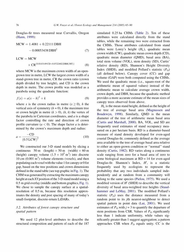
Douglas-fir trees measured near Corvallis, Oregon

(Hann, 1999):

MCW ¼ 1:4081 þ 0:22111 DBH

� 0:00053438 DBH2 (7)

LCW ¼ MCW

� CRð0:0143149 CDþ0:0722402ðDBH=HTÞÞ (8)

where MCW is the maximum crown width of an open-

grown tree in metre, LCW the largest crown width of a

stand-grown tree in metre, CR the crown ratio (crown

depth divided by tree height), and CD is the crown

depth in metre. The crown profile was modeled as a

parabola using the quadratic function:

f ðxÞ ¼ aðx � hÞ2 þ k (9)

where x is the crown radius in metre (x � 0), h the

vertical axis of symmetry (h = 0), k the maximum tree

or crown height in metre (k > 0), (h, k) the vertex of

the parabola in Cartesian coordinates, and a is a shape

factor controlling the rate and direction of crown

profile curvature (a < 0). The shape factor a is deter-

mined by the crown’s maximum depth and radius:

a ¼ �CD

ð0:5 LCWÞ2(10)

We constructed our 3-D stand models by slicing a

continuous 50 m (length) � 50 m (width) � 60 m

(height) canopy volume (1.5 � 105 m3) into discrete

10 cm (0.001 m3) volume elements (voxels), and then

populating eachvoxelwith thevalue1 forcanopyor0 for

gap, based on the tree positions and crown dimensions

defined in the stand table (see top graphic in Fig. 1). The

CHM was generated by extracting the maximum canopy

height at each XY position of the 3-D stand model using a

0.5 m grid overlay (middle and bottom graphics, Fig. 1).

We chose to sample the canopy surface at a spatial-

resolution of 0.5 m, because this resolution approx-

imates the density and post spacing of many of today’s

small-footprint, discrete-return LiDARs.

3.2. Attributes of forest canopy structure and

spatial pattern

We used 12 plot-level attributes to describe the

structural composition and pattern of each of the 187

simulated 0.25 ha CHMs (Table 2). Ten of these

attributes were calculated directly from the stand

tables, while the remaining two were extracted from

the CHMs. Those attributes calculated from stand

tables were Lorey’s height (HL), quadratic mean

crown width (CW), quadratic mean crown depth (CD),

quadratic mean diameter (QMD), basal area (BA),

total stem volume (VOL), stem density (SD), Curtis’

relative density (RD), Shannon’s Height Diversity

Index (SHDI), and modified Pollard’s statistic (PO)

(all defined below). Canopy cover (CC) and gap

volume (GAP) were both computed using the CHMs.

We used the quadratic mean (i.e., square-root of the

arithmetic mean of squared values) instead of the

arithmetic mean to calculate average crown width,

crown depth, and DBH, because the quadratic method

provides a more accurate estimate of the mean sizes of

canopy trees observed from above.

HL is the mean stand height, defined as the height of

the tree of average basal area (Magnussen and

Boudewyn, 1998). Similarly, QMD is the mean

diameter of the tree of arithmetic mean basal area

(Curtis and Marshall, 2000). BA, VOL, and SD are

frequently used estimates of stand occupancy mea-

sured on a per hectare basis. RD is a diameter-based

measure of stand density developed for even-aged

coastal Douglas-fir, commonly defined as the average

area available to the tree of average basal area relative

to either an open-grown condition or ‘‘normal’’ stand

density (Curtis, 1982). RD varies along a continuous

scale ranging from zero for a basal area of zero to

some biological maximum at RD = 14 for even-aged

Douglas-fir. Shannon’s Index, H0, is a statistic

frequently used by ecologists to represent the

probability that any two individuals sampled inde-

pendently and at random from a community will

belong to the same species (Pielou, 1975). We used a

modified version of H0 (SHDI) to describe the vertical

diversity of basal area-weighted tree heights (Staud-

hammer and LeMay, 2001). The modified Pollard’s

statistic (PO) uses the distance measured from a

random point to its jth nearest-neighbour to detect

spatial pattern in point data (Lui, 2001). We used

estimates of PO with j = 3 to quantify the departure of

stem positions from CSR. Values of PO significantly

less than 1 indicate uniformity, while values sig-

nificantly greater than 1 suggest aggregation; a pattern

approaches CSR when PO equals unity. CC is the

G.W. Frazer et al. / Forest Ecology and Management 214 (2005) 65–90 77

Table 2

Formulae for plot-level attributes used to describe forest canopy structure

Attribute (unit) Formula

Lorey’s height (m)HL ¼

Pn

i¼1d2

i hiPn

i¼1d2

i

Quadratic mean (m, cm)QM ¼

ffiffiffiffiffiffiffiffiffiffiffiffiffiffiffiffiffiffi1n

Pni¼1b2

i

qBasal area (m2/ha) BA ¼ p

40000

� �� 1

a

Pni¼1d2

i

� �Total volume (m3/ha) VOL ¼ 1

a

Pni¼3

13p 0:5di

100

� �2hi

Stem density (n/ha) SD ¼ na

Curtis’ relative density (m2/(ha/cm)) RD ¼ BAQMD0:5

Shannon’s Height Diversity Index SHDI ¼ �PH

z¼1 pz ln pz

Pollard’s statisticPO ¼ 12l2v v ln

Pv

k¼1x2

kl=vð Þ�

Pv

k¼1lnðx2

klÞ½

ð6lvþvþ1Þðv�1Þ

Canopy cover (%) CC ¼ 1 � ng

ngþnc

h i� 100

Gap volume (%)GAP ¼

Ps

q¼1

Pt

r¼1ðhmax�hqrÞPs

q¼1

Pt

r¼1hmax

" #� 100

Note: n, s, t, and v are total number of samples; di is the diameter at breast height (DBH, cm) of tree i; hi is the height (m) of tree i; bi is the crown

width (m), crown depth (m), or DBH (cm) of tree i; a is the sample plot area (a = 0.25 ha in this study); QMD is the quadratic mean diameter

(cm); pz is the proportion of basal area found in each height class z, and H is the total number of height classes (2 m height classes were used in

this study); xkl is the linear distance from the kth random point to its lth nearest-neighbour; l is the first to third nearest-neighbour (stem position)

to random point k; v is the total number of random points k overlaid on the stem map (k = 175 in this study); ng is the total number of grid-cells

with a canopy height � 2 m (classified as ground); nc is the total number of grid-cells with a canopy height > 2 m (classified as canopy); hmax is

the maximum canopy height (m) within the sample plot, and hqr is the canopy height at column q and row r of the canopy height model.

fraction of horizontal ground surface covered by the

vertical projection of tree crowns (Jennings et al.,

1999). In this study, CC was estimated as the

percentage of heights in the CHM greater than some

arbitrary height threshold (i.e., 2 m; Brokaw, 1982).

GAP is the empty intercrown space that exists between

the height of the tallest tree and the top of the outer

canopy surface, expressed as a percentage of the total

gap plus canopy volumes. Thus, GAP is the

volumetric equivalent of the intercrown canopy gap

fraction.

3.3. Statistical analyses

We used principal component analysis, Pearson

correlation, and linear and non-linear regression

analyses to facilitate the comparison and interpreta-

tion of the scale-dependent lacunarity statistics

generated for each of the 187 simulated canopies.

PCA was specifically used to create a smaller number

of uncorrelated composite variables (components)

from a linear combination of the lacunarity statistic

estimated at different spatial scales. Pearson correla-

tion and regression analyses were used to examine the

statistical relationship between each of these new

synthetic components and the 12 attributes of stand

structure and spatial pattern described above. Princi-

pal components were extracted directly from a

correlation matrix derived from an original data table

that consisted of n sample units (187 rows) by p

variables (10 columns). Where, p is one of nine scale-

dependent estimates of lacunarity L(r) measured at

approximately equal-log intervals of box size r (r = 1,

2, 3, 5, 9, 15, 24, 40, 66 in grid-cell units), and n

identifies the corresponding CHM for which these p

variables have been measured. The 10th variable that

we included in the main data table was a simple

integrated measure of cross-scale spatial heterogene-

ity, computed as the sum of the normalized lacunarity

statistic estimated at 9 discrete box sizes r:

LTOTAL ¼ 1

Lð1ÞX

LðrÞ (11)

where L(r) is the lacunarity statistic computed at the

nine box sizes listed above, and L(1) is the lacunarity

statistic estimated for box size r = 1. Small values of

G.W. Frazer et al. / Forest Ecology and Management 214 (2005) 65–9078

LTOTAL (<3.25) generally indicate uniformity or ran-

domness in canopy heights at coarser spatial scales,

while larger values (>4.25), in contrast, denote the

presence of spatial structure at coarser scales. Theses

two values of LTOTAL correspond to the 25th and 75th

percentiles of the sampled statistic, respectively. We

transformed all 10 variables independently of one

another using a rank-preserving (monotonic) power

transformation to improve linearity and normality. We

subsequently rescaled each of the transformed vari-

ables to a mean of 0 and variance of 1, so that all 10

variables had equivalent weight in the PCA. We used

PC-ORD Version 4.27 (McCune and Mefford, 1999)

for PCA and SYSTAT Version 10.2 for correlation and

regression analyses. All other spatial modeling and

analysis software used in this study was developed by

the senior author.

4. Results

4.1. Structural characteristics of the simulated

3-D stand models and derived CHMs

All four stand classes (i.e., Short, Medium, Tall,

and Natural) exhibited substantial variation in

structural composition and spatial pattern, thus

contributing to marked overlap between most classes

for many of the 12 attributes of stand and canopy

structure (Fig. 3). There were, however, a number of

distinct structural characteristics that distinguished

these four stand classes from one another. For

example, the Short class had the lowest median and

narrowest range of HL, CW, CD, QMD, BA, VOL, and

SHDI, and also showed the greatest variation in SD,

CC, and PO. Approximately 25% of the stand models

found within the Short class had PO values that

exceeded 4, indicating that some CHMs in this class

had substantially higher levels of nearest-neighbour

spatial aggregation than those in other stand classes.

Simulated CHMs within the Medium class also

exhibited substantial variation in CC, PO, and SHDI,

and had the greatest range of GAP values. Although

this stand class was limited in its range of HL, it still

displayed moderate variability in CW and CD. The

Tall class contained CHMs with the largest HL, CW,

CD, and QMD, and also revealed substantial variation

in CW, CD, QMD, BA, VOL, RD, CC, and GAP. RD,

CC, and GAP all varied considerably within the Tall

class, despite the narrow range and low median value

of SD. The Natural class produced the highest median

BA, VOL, RD, SHDI, and CC; however, the range of

SHDI and CC within this class was extremely limited,

and more so than any other stand class. The Natural

class also had the lowest median and narrowest range

of GAP, because of its very high median CC and

generally uniform to random (0.21 � PO � 1.38) stem

point patterns.

4.2. Scale-dependent estimates of the lacunarity

statistic

Minimum, maximum, and median estimates of the

lacunarity statistic computed at box size r = 1 for all

187 simulated CHMs were 1.01, 11.92, and 1.54,

respectively. The lacunarity statistic was always at its

maximum value at the finest scale of measurement

(i.e., box size r = 1), indicating that all CHMs

generally became more spatially homogeneous at

coarser measurement scales. The rate and pattern of

decline in lacunarity at larger measurement scales was

solely determined by the canopies’ hierarchical spatial

structure and scale-dependent patchiness (i.e., the

clumping of foliage into individual crowns and then

into groups of crowns of variable sizes and patterns).

The Short class exhibited the widest range of

lacunarity estimates across the first seven measure-

ment scales (0.5 � s � 12 m), indicating substantial

variation in the magnitude and pattern of spatial

aggregation at these finer spatial scales (Fig. 4). In

contrast, the Natural class had the narrowest range and

lowest median value of the lacunarity statistic at all

nine measurement scales, largely because of their

characteristic high levels of canopy cover (density)

and the limited size and depth of intercrown gaps. The

Medium class also revealed substantial variation in

lacunarity across the first five measurement scales

(0.5 � s � 4.5 m), but the median and range of the

lacunarity statistic were more similar to the Short and

Tall classes at coarser spatial scales.

Minimum, maximum, and median values of

LTOTAL computed in this study were, respectively,

1.74, 5.56, and 3.89. Larger values of LTOTAL

generally denote both the presence and persistence

of spatial structure or aggregation at increasingly

coarser measurement scales. The Tall class displayed

G.W. Frazer et al. / Forest Ecology and Management 214 (2005) 65–90 79

Fig. 3. Boxplots summarizing the frequency distributions of 12 different attributes of stand and canopy structure stratified by stand class. The

lower and upper bounds of the boxplot represent the 25th and 75th percentiles, the horizontal line within the box is the median value of the

distribution, and box whiskers identify the range of extreme values.

the largest median value of LTOTAL (4.29), followed in

descending order by the Natural (3.92), Medium (3.60),

and Short (3.22) classes. The Medium class revealed the

greatest range of variation in LTOTAL (1.74 �LTOTAL � 5.35), while the Natural class showed the

least amount of variation (3.09 �LTOTAL � 4.60). The

larger values of LTOTAL exhibited by the Tall and

Natural classes are due to their coarser-scale structure

(bigger crowns and gaps) and greater variation in crown

and gap sizes. The wide variation in LTOTAL associated

G.W. Frazer et al. / Forest Ecology and Management 214 (2005) 65–9080

Fig. 4. Boxplots showing the frequency distributions of the lacunarity statistic L(r) stratified by linear box size r and stand class. Measurement

scale is identified in grid-cell units on the Y-axis and as an absolute unit of measure (metre) in the top left-hand corner of each graph. LTOTAL is a

simple integrated measure of cross-scale spatial heterogeneity.

G.W. Frazer et al. / Forest Ecology and Management 214 (2005) 65–90 81

Table 3

Principal component loadings and Pearson correlations between principal components and lacunarity statistics

Attributea PC1 PC2

Loadingsb R R2 Loadingsb R R2

L(1) �0.317 �0.946 0.896 0.337 0.321 0.103

L(2) �0.320 �0.956 0.913 0.306 0.292 0.085

L(3) �0.323 �0.964 0.928 0.278 0.264 0.070

L(5) �0.330 �0.978 0.956 0.212 0.202 0.041

L(9) �0.333 �0.994 0.988 0.078 0.074 0.006*

L(15) �0.333 �0.995 0.990 �0.058 �0.055 0.003*

L(24) �0.329 �0.984 0.969 �0.157 �0.150 0.022

L(40) �0.322 �0.963 0.927 �0.222 �0.211 0.045

L(66) �0.311 �0.930 0.865 �0.243 �0.231 0.053

LTOTAL �0.236 �0.704 0.496 �0.727 �0.689 0.474a All attributes except LTOTAL were log transformed.b Principal component loadings (eigenvector coefficients) of the original variables.* Not significant at 0.05 level.

with Medium class was due to substantial spatial

variability in vertical and horizontal canopy structure

as indicated by the broad ranges of CC, GAP, SHDI,

and PO. The range of LTOTAL estimates was limited

in the Natural class, due to very high levels of

canopy cover, the limited size and depth of

intercrown gaps, and their predominantly random

to uniform stem patterns.

Fig. 5. Ordination diagram showing the distribution of sample points in re

separated sample units in the multi-dimensional space of the original descr

likely to have similar scale-dependent spatial patterns. The labels marked

CHMs shown in Fig. 7.

4.3. Ordination of scale-dependent lacunarity

data using PCA

The first two principal components accounted for

98.4% of the total variance found in the original scale-

dependent lacunarity data, with 89.3 and 9.1% of total

variance explained by the first (PC1) and second (PC2)

principal components, respectively. The third princi-

duced ordination space. PCA attempts to preserve the distances that

iptors, therefore CHMs located in close proximity of one another are

P1, P3, etc., correspond to the 15 selected examples of simulated

G.W. Frazer et al. / Forest Ecology and Management 214 (2005) 65–9082

Fig. 6. Overlay plot summarizing the relationship between attributes of stand and canopy structure and the first and second principal

components. The diameter of the circular plot symbol is proportional to magnitude of the attribute. Gradients of variation in these structural

attributes are defined by a monotonic increase or decrease in symbol size. The direction of this change defines the statistical association between

the variable and each of the two principal components.

G.W. Frazer et al. / Forest Ecology and Management 214 (2005) 65–90 83

Table 4

Pearson correlations between principal components and attributes of

stand structure

Attributes PC1 PC2

R R2 R R2

HL 0.061 0.004* �0.703 0.495

CWa 0.164 0.027 �0.629 0.395

CDa 0.179 0.032 �0.660 0.436

QMDa 0.143 0.020* �0.663 0.440

BAa 0.669 0.448 �0.682 0.465

VOLa 0.521 0.271 �0.739 0.546

SDa 0.594 0.352 0.107 0.011*

RDa 0.764 0.584 �0.595 0.354

SHDIb 0.109 0.012* �0.652 0.425

POa �0.479 0.229 �0.046 0.002*

CC 0.921 0.848 �0.320 0.102

GAP �0.918 0.842 0.294 0.087a Transformed using natural log.b Zero values of SHDI excluded from correlation.* Not significant at 0.05 level.

pal component (PC3) accounted for only 1.1% of the

total variance, and was therefore excluded from

further analyses. PC1 had a strong negative correlation

with the lacunarity statistic at all nine discrete spatial

scales (0.865 � R2 � 0.990), and moderate negative

correlation (R2 = 0.496) with LTOTAL (Table 3). The

sign and strength of the Pearson coefficient of

correlation, R, between the scale-dependent lacunarity

statistic and PC2 declined from a low positive value of

R = 0.321 at scale r = 1, to R = 0.074 at scale r = 7,

and finally to a small negative value of R = �0.231 at

scale r = 60. LTOTAL was also moderately negatively

correlated with PC2 (R2 = 0.474). Three main con-

clusions were drawn from these patterns of correla-

tion. First, strong negative correlations between PC1

and lacunarity at all spatial scales indicated that PC1

scores declined as the magnitude of the lacunarity

statistic increased. Second, PC2 scores increased and

decreased when simulated CHMs were dominated by

fine-scale and coarse-scale spatial patterns, respec-

tively. Third, PC1 and PC2 scores both declined when

the cross-scale spatial heterogeneity (LTOTAL) exhib-

ited by the CHMs increased.

A scatterplot of PC1 versus PC2 scores revealed

the spatial distribution of simulated CHMs in reduced

ordination space (Fig. 5). PCA attempts to preserve

the relative Euclidean distances that separated sample

units in the multi-dimensional space of the original

descriptors (Legendre and Legendre, 1998). There-

fore, simulated CHMs found at close proximity in

ordination space will likely have lacunarity curves of

similar magnitude and shape, while those far apart

will have curves that are dissimilar in these same two

characteristics. Despite the substantial overlap among

the 4 different stand classes for many of the 12

attributes of stand and canopy structure, each stand

class occupied a relatively distinct region of ordina-

tion space. For example, stand classes tended to

stratify vertically, with the Short class dominating the

top of the scatterplot, the Medium class in the middle,

and the Tall and Natural classes on the bottom. The

Short, Medium, and Tall classes occupied the largest

regions of ordination space, largely because these

classes varied widely in CC, GAP, SHDI, and PO. In

contrast, the Natural class was limited in its ranges of

these same four attributes, and therefore filled a

relatively small, but unique region of ordination

space.

4.4. Correlations between principal components,

lacunarity, and attributes of forest stand and

canopy structure

PCA uncovered a number of gradients in the

original lacunarity dataset that were associated with

the vertical and horizontal patchiness (texture) of the

canopy and other more specific size- and density-

related attributes of stand and canopy structure

(Fig. 6). We found that PC1 was strongly positively

correlated with estimates of CC (R2 = 0.848) and

negatively correlated with GAP (R2 = 0.842)

(Table 4). For example, P99 and P100 are two paired

examples of simulated CHMs having the highest PC1

scores, while P19 and P43 are characterized by the two

lowest PC1 scores (Fig. 7). P99 recorded the lowest

L(1) statistic (1.01), highest CC (99.99%), and lowest

GAP (10.2%) of all simulated CHMs, while P43, in

contrast, had the highest L(1) statistic (11.92), lowest

CC (11.10%), and highest GAP (94.3%). Regression

analyses revealed a strong negative linear relationship

between the logarithm of L(1) and logarithm of CC

(R2 = 0.982), and a strong positive exponential

relationship between the logarithm of L(1) and

GAP (R2 = 0.959). PC1 was poorly correlated with

many of the size-related attributes such as HL, CW,

CD, and QMD (0.004 � R2 � 0.032), but positively

correlated (0.271 � R2 � 0.584) with density-related

attributes of stand structure, such as RD, BA, SD, and

G.W. Frazer et al. / Forest Ecology and Management 214 (2005) 65–9084

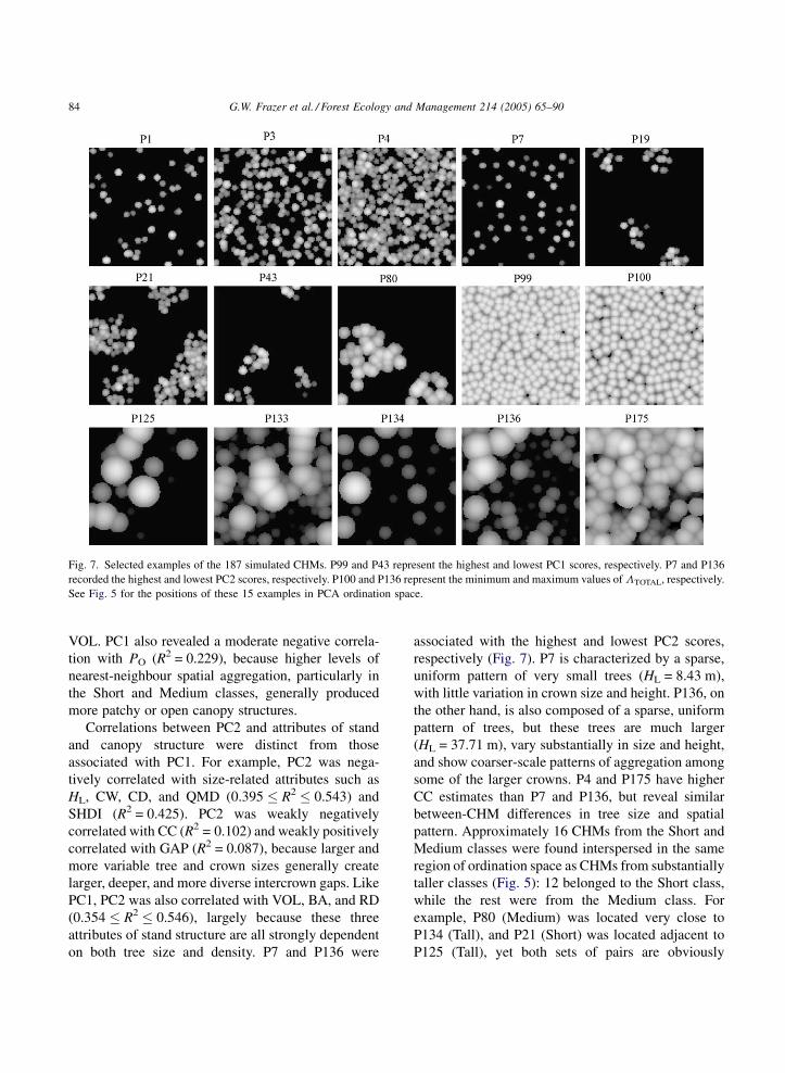
Fig. 7. Selected examples of the 187 simulated CHMs. P99 and P43 represent the highest and lowest PC1 scores, respectively. P7 and P136

recorded the highest and lowest PC2 scores, respectively. P100 and P136 represent the minimum and maximum values of LTOTAL, respectively.

See Fig. 5 for the positions of these 15 examples in PCA ordination space.

VOL. PC1 also revealed a moderate negative correla-

tion with PO (R2 = 0.229), because higher levels of

nearest-neighbour spatial aggregation, particularly in

the Short and Medium classes, generally produced

more patchy or open canopy structures.

Correlations between PC2 and attributes of stand

and canopy structure were distinct from those

associated with PC1. For example, PC2 was nega-

tively correlated with size-related attributes such as

HL, CW, CD, and QMD (0.395 � R2 � 0.543) and

SHDI (R2 = 0.425). PC2 was weakly negatively

correlated with CC (R2 = 0.102) and weakly positively

correlated with GAP (R2 = 0.087), because larger and

more variable tree and crown sizes generally create

larger, deeper, and more diverse intercrown gaps. Like

PC1, PC2 was also correlated with VOL, BA, and RD

(0.354 � R2 � 0.546), largely because these three

attributes of stand structure are all strongly dependent

on both tree size and density. P7 and P136 were

associated with the highest and lowest PC2 scores,

respectively (Fig. 7). P7 is characterized by a sparse,

uniform pattern of very small trees (HL = 8.43 m),

with little variation in crown size and height. P136, on

the other hand, is also composed of a sparse, uniform

pattern of trees, but these trees are much larger

(HL = 37.71 m), vary substantially in size and height,

and show coarser-scale patterns of aggregation among

some of the larger crowns. P4 and P175 have higher

CC estimates than P7 and P136, but reveal similar

between-CHM differences in tree size and spatial

pattern. Approximately 16 CHMs from the Short and

Medium classes were found interspersed in the same

region of ordination space as CHMs from substantially

taller classes (Fig. 5): 12 belonged to the Short class,

while the rest were from the Medium class. For

example, P80 (Medium) was located very close to

P134 (Tall), and P21 (Short) was located adjacent to

P125 (Tall), yet both sets of pairs are obviously

G.W. Frazer et al. / Forest Ecology and Management 214 (2005) 65–90 85

dissimilar in stand structure and pattern (Fig. 7).

Interestingly, all of these 16 plots exhibited an

unusually strong hierarchical arrangement of crowns

into discrete randomly distributed clusters (2.76 �PO � 7.95; see Fig. 6J).

5. Discussion and conclusions

Lacunarity is a quantitative measure of texture

increasingly used to characterize the cross-scale

heterogeneity associated with a broad range of

spatiotemporal phenomena. We used the lacunarity

statistic estimated at 9 discrete measurement scales to

examine the spatial heterogeneity found in the outer

canopy surface of 187 simulated CHMs. The lacunarity

statistic has a theoretical range from a minimum value

of 1 to some infinite positive number, where 1

represents spatial homogeneity (zero spatial variance),

and increasingly larger values of the statistic imply

increasing heterogeneity. We found that the magnitude

of the lacunarity statistic was strongly associated with

canopy cover and gap volume, while the pattern of

decline in lacunarity across discrete measurement

scales was related to many size- and density-related

attributes of stand and canopy structure and their

diverse vertical and horizontal spatial distributions.

These general findings are supported by other published

studies that have reported a strong positive correlation

between stand-level canopy texture or patchiness and

scale-dependent estimates of lacunarity (Sun and

Ranson, 1998; Weishampel et al., 2000).

We used PCA explicitly to uncover gradients of

scale-dependent spatial heterogeneity in the surface

pattern and structure of our simulated CHMs. PCA

revealed that a substantial portion (98.34%) of the total

variance contained in the 10 dimensions of the original

lacunarity dataset could be explained by 2 synthetic,

orthogonal components. The first component (PC1)

captured 89.3% of the total variance in the original

lacunarity data, while the second (PC2) accounted for

the remaining 9.1%. Pearson correlation showed that

PC1 scores were largely determined by the magnitude

of the lacunarity statistic estimated at each of nine

discrete measurement scales (0.865 � R2 � 0.990). In

contrast, PC2 showed very little correlation with the

lacunarity statistic at any of the measurement scales

(0.003 � R2 � 0.103), and was instead related to rates

of decline, subtle breaks in slope, and other scale-

dependent variations in the shape of the lacunarity

curve. Further analyses showed that PC1 and the

magnitude of the lacunarity statistic at box size r = 1

were both strongly correlated with canopy cover and

gap volume, while PC2 was negatively correlated with

size-related attributes of stand structure (i.e., mean

height, crown width and depth, DBH, and height

diversity). Both PC1 and PC2 were moderately

correlated with density-related attributes of stand

structure (i.e., volume, basal area, and relative density),

because all of these forest measurements are influenced

by both tree size and stem density. Even though most of

the variance (approximately 75%) found in the original

lacunarity dataset could be explained solely by canopy

cover or gap volume, a sufficient amount of variance

still remained to effectively separate CHMs in

ordination space along other diverse gradients of forest

canopy structure and scale-dependent spatial pattern.

Detailed 3-D views of the forest canopy looking

down from above have helped to reshape our thinking

about canopy structure and the ways in which it can be

quantified and studied. Measures of canopy cover have

traditionally been regarded as dichotomous (i.e.,

canopy or gap), rather than reflecting the true

continuous nature of canopy height, depth, density,

porosity, and pattern (Lieberman et al., 1989; Dial

et al., 2004). In this study, the forest canopy was

treated as a continuous surface of varying height,

where gaps were physically defined by the empty

spaces of variable depth, width, and shape that

separated neighbouring crowns. Consequently, the

hierarchical arrangement of canopy elements in both

vertical and horizontal spatial domains determined the

size, shape, and patchy distribution of filled and empty

canopy spaces, and therefore the kind, magnitude, and

scale of spatial heterogeneity. Two distinctively

different, yet complementary gradients of spatial

heterogeneity emerged from analyses of these canopy

height data. The stronger of these two gradients

reflected the continuous variation in canopy cover and

intercrown gap volume, while a second, more subtle

gradient was associated with the array of possible

vertical and horizontal spatial configurations that

might define any one measure of canopy cover.

Canopy cover and other related measures of site

occupancy (e.g., stem density, basal area, volume,

etc.) are well known to be negatively correlated with

G.W. Frazer et al. / Forest Ecology and Management 214 (2005) 65–9086

mean values of the understory light environment

(Baldocchi and Collineau, 1994; Lieffers et al., 1999).

Vertical and horizontal spatial distributions of canopy

cover, on the other hand, play key roles in structuring

spatiotemporal patterns of light and other critical

forest resources (Trichon et al., 1998; Wirth et al.,

2001; Parker et al., 2002), and have therefore been

considered an important driver of many key ecosystem

processes and functions, including stand dynamics

(Canham et al., 1994; Nicotra et al., 1999; Van Pelt

and Franklin, 2000; Herwitz et al., 2000), stand

productivity, niche diversification, and biodiversity

(Franklin et al., 2002; Carey, 2003; Ishii et al., 2004).

Spatial characteristics of canopy structure are also

known to vary markedly throughout stand succession,

with the most substantial and unique patterns of

vertical and horizontal spatial heterogeneity often

occurring in the later stages of stand development

(Brown and Parker, 1994; Franklin and Van Pelt, 2004;

Parker and Russ, 2004).

The kinds of spatiotemporal pattern that we are able

to observe in nature are constrained by the grain

(resolution) and extent of our measurements (Marceau

et al., 1994; Gardner, 1998; Dale, 1999). The horizontal

extent of our simulated forest canopy view was

restricted to 50 m � 50 m (0.25 ha), and the grain of

our measurements ranged from 0.5 to 33 m. We would,

however, expect different scale-dependent patterns of

spatial heterogeneity to emerge if the grain or extent of

our models and measurements of lacunarity were

reduced or enlarged. Larger sample plots, for example,

are generally expected to exhibit substantially more

spatial heterogeneity in canopy structure over the same

fixed range of measurement scales than smaller plots

(Zenner, 2005). In real forests, stand structure and

species composition vary considerably both locally and

regionally in response to fine- and coarse-scale

variations in edaphic factors, disturbance regime, and

successional processes (Franklin et al., 2002). Conse-

quently, increasing the spatial extent over which canopy

heights and lacunarity are measured is likely to reveal

different scale-dependent patterns of spatial hetero-

geneity. It is, therefore, imperative that both the grain

and extent of spatial observation, measurement, and

analysis match as closely as possible the ecological

phenomenon of interest.

Accurate, high-spatial-resolution (<1 m) canopy

heights can be readily acquired with airborne LiDAR

instruments (Lefsky et al., 2002; St-Onge et al., 2003)

or from high-resolution aerial photos and digital

photogrammetry (Miller et al., 2000). We propose two

different potential sampling strategies to extract fine-

scale estimates of lacunarity from a regularly spaced,

rectangular array of quantitative canopy heights. First,

a sample window (quadrat) of fixed size and geometry

could be moved in either an overlapping or non-

overlapping manner to cover an entire array of canopy

heights. The sample quadrat may be equivalent in size

to the 50 m � 50 m (0.25 ha) horizontal footprint of

the simulated CHMs used in this study, or it could be

smaller or larger depending on the objectives of the

research and the grain and extent of the data. At each

quadrat position, the lacunarity statistic is then

estimated at a number of discrete spatial scales within

the bounds of the quadrat. Alternatively, forest cover

maps identifying the distinct boundaries of individual

stands may provide the spatial context for undertaking

a stratified-random-sampling approach. For example,

sample quadrats of some predetermined size could be

randomly placed within the confines of each stand

boundary to avoid the arbitrariness and boundary

issues inherent in the first sampling approach. Spatial

boundaries or ecotones can, however, represent a

legitimate and interesting ecological phenomenon.

Therefore, both sampling strategies will likely have

merit depending on the study objectives.

Lacunarity provides a simple conceptual and

methodological framework to study the scale-depen-

dent spatial heterogeneity of forest canopies. Ordina-

tion techniques, especially those that are

unconstrained and distance-preserving, facilitate the

comparison of cross-scale spatial heterogeneity by

separating CHMs in reduced ordination space along

unique gradients of pattern and structure. When used

together, these two techniques provide substantial

opportunity for forest scientists to study a broad range

of ecological and forest management problems. For

example, pooling scale-dependent lacunarity esti-

mates collected from local managed and natural

forests into a single statistical ordination would allow

forest managers to assess the potential impact of

specific silvicultural practices on both fine- and

coarse-scale patterns of spatial heterogeneity. Ordina-

tion diagrams are helpful in this respect, because they

show the overall variation of points in sample space, as

well as identify both the distance and direction

G.W. Frazer et al. / Forest Ecology and Management 214 (2005) 65–90 87

separating any two sample units or classes of interest.

Target plots representing some kind of ideal structural

condition or habitat may be identified prior to analysis,

as a way to establish a frame of reference to compare

all other sample units in reduced ordination space.

The current shift towards an ecosystem-based

approach to sustainable forest management in North

America has created a demand for cost-effective forest

measurement and monitoring technologies, analytical

methods, and relevant scientific data (Lindenmayer and

Franklin, 2002). We expect that our novel methodo-

logical approach could be used in conjunction with

high-spatial-resolution airborne LiDAR data or digital

photogrammetry to support a broad range of ecological

applications. For example, this method could be used to

study the fine-scale spatial heterogeneity of ‘natural’

forest canopies as a blueprint for developing new stand-

level gap- or retention-based silvicultural systems (see

Coates and Burton, 1997). Second, homogeneous or

heterogeneous forest patterns may be identified as

targets for structural restoration or retention, respec-

tively (see Carey, 2003). Third, this technique could be

used to monitor stand-level spatial aspects of forest

canopies for adaptive forest management and certifica-

tion purposes (see Kremsater et al., 2003). Fourth,

quantitative estimates of scale-dependent spatial

heterogeneity may help to identify unique ecosystems

or wildlife habitats (e.g., riparian or old-growth forests,

etc.) suitable for designation as special management

areas or reserves. Fifth, this method would facilitate the

segmentation of LiDAR or other kinds of remotely

sensed data into unique structural classes based on

quantitative estimates of fine-scale spatial heterogene-

ity. Last, because lacunarity is well-correlated with

more traditional measurements of stand structure (i.e.,

canopy cover, height, crown size, volume, basal area,

and relative density), we expect that synthetic variables

generated by PCA from the original lacunarity dataset

may become useful predictors of stand structure in

regression analyses when combined with some

percentile of canopy height.

Studies in ecology, spatial pattern analysis, and

remote sensing have demonstrated that there is no

single, ‘optimum’ scale or window size that can be

prescribed to analyze the complex spatial patterns and

hierarchical structure of heterogeneous forest canopies

(Marceau et al., 1994; Coburn and Roberts, 2004). In

this study, we found that the spatial heterogeneity

associated with canopy heights varied substantially

with measurement scale, and it was this cross-scale

pattern of variation that distinguished one CHM from

another. Lacunarity analysis appears to offer several

advantages over other spatial statistical approaches.

First, lacunarity is a multi-scaled method and does not

depend on the existence of a single, ‘optimum’

measurement scale. Second, lacunarity does not require

the unlikely assumption of spatial stationarity to remain

unbiased. Third, lacunarity is computed simply and

efficiently, and is easily applied to binary or quantitative

datasets of any Euclidean dimension. Last, when

applied to 2-D quantitative canopy heights, lacunarity

becomes an integrated, scale-dependent measure of

vertical and horizontal spatial heterogeneity. Further

research is required to understand how these statistical

estimates and gradients of measured heterogeneity

relate to other ecologically relevant patterns of forest

composition, structure, and function.

Acknowledgements

We thank Drs. Richard Fournier and Ken Lertzman

for many insightful comments and discussions during

the preparation of this manuscript. Drs. Fangliang He

and Roy Plotnick provided technical advice on

modeling spatial point processes and the application

of lacunarity analysis to quantitative data, respectively.

We also thank the two anonymous reviewers for their

helpful suggestions on ways to improve the manuscript.

Funding for this research was provided by British

Columbia Forest Innovation Investment, Science

Council of British Columbia, Weyerhaeuser BC Coastal

Group, Canadian Forest Service (Pacific Forestry

Centre, Victoria, BC), and the British Columbia

Advanced Systems Institute under an industrial partner-

ship grant sponsored by Terra Remote Sensing Inc.,

Sidney, BC.

References

Allain, C., Cloitre, M., 1991. Characterizing the lacunarity of

random and deterministic fractal sets. Phys. Rev. A 44, 3552–

3558.

Baldocchi, D., Collineau, S., 1994. The physical nature of solar

radiation in heterogeneous canopies: spatial and temporal attri-

butes. In: Caldwell, M.M., Pearcy, R.W. (Eds.), Exploitation of

G.W. Frazer et al. / Forest Ecology and Management 214 (2005) 65–9088

Environmental Heterogeneity by Plants: Ecophysiological Pro-

cesses Above- and Below Ground. Academic Press, San Diego,

pp. 21–71.

Bartemucci, P., Coates, K.D., Harper, K.A., Wright, E.F., 2002. Gap

disturbances in northern old-growth forests of British Columbia,

Canada. J. Veg. Sci. 13, 685–696.

Blumenfeld, R., Mandelbrot, B.B., 1997. Levy dusts, Mittag–Leffler

statistics, mass fractal lacunarity, and perceived dimension.

Phys. Rev. E 56, 112–118.

Bradshaw, G.A., Spies, T.A., 1992. Characterizing canopy gaps in

forests using wavelet analysis. J. Ecol. 80, 205–215.

Brokaw, N.V.L., 1982. The definition of treefall gap and its effect on

measures of forest dynamics. Biotropica 14, 158–160.

Brown, M.J., Parker, G.G., 1994. Canopy light transmittance in a

chronosequence of mixed-species deciduous forests. Can. J. For.

Res. 24, 1694–1703.

Caldwell, M.M., Pearcy, R.W., 1994. Exploitation of Environmental

Heterogeneity by Plants: Ecophysiological Processes Above-

and Below Ground. Academic Press, San Diego.

Canham, C.D., Finzi, A.C., Pacala, S.W., Burbank, D.H., 1994.

Causes and consequences of resource heterogeneity in forests:

interspecific variation in light transmission by canopy trees. Can.

J. For. Res. 24, 337–349.

Carey, A.B., 2003. Biocomplexity and restoration of biodiversity

in temperate coniferous forests: inducing spatial heteroge-

neity with variable-density thinning. Forestry 76, 127–

136.

Cescatti, A., 1998. Effects of needle clumping in shoots and crowns

on the radiative regime of a Norway spruce canopy. Ann. Sci.

For. 55, 89–102.

Chen, J., Bradshaw, G.A., 1999. Forest structure in space: a

case study of an old growth spruce-fir forest in Changbaishan

Natural Reserve, PR China. For. Ecol. Manage. 120, 219–

233.

Chen, J., Saunders, S.C., Crow, T.R., Naiman, R.J., Brosofske, K.D.,

Mroz, G.D., Brookshire, B.L., Franklin, J.F., 1999. Microclimate

in forest ecosystem and landscape ecology. BioScience 49, 288–

297.

Cheng, Q., 1997. Multifractal modeling and lacunarity analysis.

Math. Geol. 29, 919–932.

Coates, K.D., Burton, P.J., 1997. A gap-based approach for devel-

opment of silvicultural systems to address ecosystem manage-

ment objectives. For. Ecol. Manage. 99, 337–354.

Coburn, C.A., Roberts, A.C.B., 2004. A multiscaled texture analysis

procedure for improved stand classification. Int. J. Remote Sens.

20, 4287–4308.

Cohen, W.B., Spies, T.A., Bradshaw, G.A., 1990. Semivariograms of

digital imagery for analysis of conifer canopy structure. Remote

Sens. Environ. 34, 167–178.

Curtis, R.O., 1982. A simple index of stand density for Douglas-fir.

For. Sci. 28, 92–94.

Curtis, R.O., Marshall, D.D., 2000. Why quadratic mean diameter?

West. J. Appl. For. 15, 137–139.

Dale, M.R.T., 1999. Spatial Pattern Analysis in Plant Ecology.

Cambridge University Press, Cambridge, UK.

Dale, M.R.T., 2000. Lacunarity analysis of spatial pattern: a com-

parison. Landscape Ecol. 15, 467–478.

Dial, R., Bloodworth, B., Lee, A., Boyne, P., Heys, J., 2004. The

distribution of free space and its relation to canopy composition

at six forest sites. For. Sci. 50, 312–325.

Diggle, P.J., 2003. Statistical Analysis of Spatial Point Patterns.

Oxford University Press, New York, NY.

Drake, J.B., Weishampel, J.F., 2000. Multifractal analysis of canopy

height measures in a longleaf pine savanna. For. Ecol. Manage.

128, 121–127.

Dutilleul, P., Legendre, P., 1993. Spatial heterogeneity against

heteroscedasticity: an ecological paradigm versus a statistical

concept. Oikos 66, 152–171.

Ehleringer, J.R., Field, C.B., 1993. Scaling Physiological Processes:

Leaf to Globe. Academic Press, San Diego, CA.

Feagin, R.A., 2003. Relationship of second-order lacunarity, Hurst

exponent, Brownian motion, and pattern organization. Physica A

328, 315–321.

Fournier, R.A., Rich, P.M., Landry, R., 1997. Hierarchical charac-

terization of canopy architecture for boreal forests. J. Geophys.

Res. 102, 29445–29454.

Franklin, J.F., Spies, T.A., Van Pelt, R., Carey, A.B., Thornburgh,

D.A., Berg, D.R., Lindenmayer, D.B., Harmon, M.E., Keeton,

W.S., Shaw, D.C., Bible, K., Chen, J., 2002. Disturbances and

structural development of natural forest ecosystems with silvi-

cultural implications, using Douglas-fir as an example. For.

Ecol. Manage. 155, 399–423.

Franklin, J.F., Van Pelt, R., 2004. Spatial aspects of structural

complexity in old-growth forests. J. For. 102, 22–28.

Frazer, G.W., Trofymow, J.A., Lertzman, K.P., 2000. Canopy open-

ness and leaf area in chronosequences of coastal temperate

rainforests. Can. J. For. Res. 30, 239–256.

Gardner, R.H., 1998. Pattern, process, and the analysis of spatial

scales. In: Peterson, D.L., Parker, V.T. (Eds.), Ecological Scale:

Theory and Applications. Columbia University Press, New

York, pp. 17–34.

Geffen, Y., Meir, Y., Mandelbrot, B.B., Aharony, A., 1983. Geo-

metric implementation of hypercubic lattices with noninteger

dimensionality by use of low lacunarity fractal lattices. Phys.

Rev. Lett. 50, 145–148.

Gustafson, E.J., 1998. Quantifying landscape spatial pattern: what is

the state of the art? Ecosystems 1, 143–156.

Hann, D.W., 1999. An adjustable predictor of crown profile for

stand-grown Douglas-fir trees. For. Sci. 45, 217–225.

Henebry, G.M., Kux, H.J.H., 1995. Lacunarity as a texture measure

for SAR imagery. Int. J. Remote Sens. 16, 565–571.

Herwitz, S.R., Slye, R.E., Turton, S.M., 2000. Long-term survivor-

ship and crown area dynamics of tropical rain forest canopy

trees. Ecology 81, 585–597.

Ishii, H.T., Tanabe, S., Hiura, T., 2004. Exploring the relation-

ships among canopy structure, stand productivity, and biodi-

versity of temperate forest ecosystems. For. Sci. 50, 342–

355.

Jennings, S.B., Brown, N.D., Sheil, S., 1999. Assessing forest

canopies and understorey illumination: canopy closure, canopy

cover and other measures. Forestry 72, 59–73.

Kaluzny, S.P., Vega, S.C., Cardoso, T.P., Shelly, A.A., 1998.

S + SpatialStats, User’s Manual for Windows1 and Unix1.

Springer-Verlag, New York, NY.

G.W. Frazer et al. / Forest Ecology and Management 214 (2005) 65–90 89

Kirkpatrick, L.A., Weishampel, J.F. Quantifying spatial structure of

volumetric neutral models. Ecol. Model., in press.

Kolasa, J., Pickett, S.T.A., 1991. Ecological Heterogeneity.

Springer-Verlag, New York.

Kolasa, J., Rollo, C.D., 1991. Introduction: the heterogeneity of

heterogeneity: a glossary. In: Kolasa, J., Pickett, S.T.A. (Eds.),

Ecological Heterogeneity. Springer-Verlag, New York, pp. 1–

23.

Koukoulas, S., Blackburn, G.A., 2004. Quantifying the spatial

properties of forest canopy gaps using LiDAR imagery and

GIS. Int. J. Remote Sens. 25, 3049–3071.

Kremsater, L., Bunnell, F., Huggard, D., Dunsworth, G., 2003.

Indicators to assess biological diversity: Weyerhaeuser’s coastal

British Columbia forest project. For. Chronicle 79, 590–

601.

Lefsky, M.A., Cohen, W.B., Parker, G.G., Harding, D.J., 2002.

LiDAR remote sensing for ecosystem studies. BioScience 52,

19–30.

Legendre, P., Fortin, M.-J., 1989. Spatial pattern and ecological

analysis. Vegetatio 80, 107–138.

Legendre, P., Legendre, L., 1998. Numerical Ecology. Elsevier

Science, Amsterdam.

Lertzman, K.P., Fall, J.G., 1998. From forest stands to landscapes:

spatial scales and the roles of disturbance. In: Peterson, D.L.,

Parker, V.T. (Eds.), Ecological Scale: Theory and Applications.

Columbia University Press, New York, pp. 339–367.

Li, H., Reynolds, J.F., 1995. On definition and quantification of

heterogeneity. Oikos 73, 280–284.

Lieberman, M., Lieberman, D., Peralta, R., 1989. Forests are not just

Swiss cheese: canopy stereogeometry of non-gaps in tropical

forests. Ecology 70, 550–552.

Lieffers, V.J., Messier, C., Stadt, K.J., Gendron, F., Comeau, P.G.,

1999. Predicting and managing light in the understory of boreal

forests. Can. J. For. Res. 29, 796–811.

Lim, K., Treitz, P., Wulder, M., St-Onge, B., Flood, M., 2003.

LiDAR remote sensing of forest structure. Prog. Phys. Geogr. 27,

88–106.

Lindenmayer, D.B., Franklin, J.F., 2002. Conserving Forest Biodi-

versity: A Comprehensive Multiscaled Approach. Island Press,

Washington, DC.

Lui, C., 2001. A comparison of five distance-based methods for

spatial pattern analysis. J. Veg. Sci. 12, 411–416.

Magnussen, S., Boudewyn, P., 1998. Derivations of stand heights

from airborne laser scanner data with canopy-based quantile

estimators. Can. J. For. Res. 28, 1016–1031.

Mandelbrot, B.B., 1983. The Fractal Geometry of Nature. W.H.

Freeman and Company, New York, NY.

Manly, B.F.J., 1997. Randomization, Bootstrap and Monte Carlo

Methods in Biology. Chapman and Hall, London.

Marceau, D.J., Howarth, P.J., Gratton, D.J., 1994. Remote sensing

and the measurement of geographical entities in a forested

environment. 1. The scale and spatial aggregation problem.

Remote Sens. Environ. 49, 93–104.

McCune, B., Mefford, M.J., 1999. PC-ORD Version 4 for Win-

dows1. MjM Software Design, Gleneden, OR.

Miller, D.R., Quine, C.P., Hadley, W., 2000. An investigation of the

potential of digital photogrammetry to provide measurements of

forest characteristics and abiotic damage. For. Ecol. Manage.

135, 279–288.

Moeur, M., 1993. Characterizing spatial patterns of trees using stem-

mapped data. For. Sci. 39, 756–775.

Montgomery, R.A., Chazdon, R.L., 2001. Forest structure, canopy

architecture, and light transmittance in tropical wet forests.

Ecology 82, 2707–2718.

Nadkarni, N.M., Sumera, M.M., 2004. Old-growth forest canopy

structure and its relationship to throughfall interception. For. Sci.

50, 290–298.

Nicotra, A.B., Chazdon, R.L., Iriarte, S., 1999. Spatial heterogeneity

of light and woody seedling regeneration in tropical wet forests.

Ecology 80, 1908–1926.

Ollier, S., Chessel, D., Couteron, P., Pelissier, R., Thioulouse, J.,

2003. Comparing and classifying one-dimensional spatial pat-

terns: an application to laser altimeter profiles. Remote Sens.

Environ. 85, 453–462.

Parker, G.G., 1995. Structure and microclimate of forest canopies.

In: Lowman, M.D., Nadkarni, N.M. (Eds.), Forest Canopies.

Academic Press, Orlando, FL, pp. 73–98.

Parker, G.G., Davis, M.M., Chapotin, S.M., 2002. Canopy light

transmittance in Douglas-fir—western hemlock stands. Tree

Physiol. 22, 147–157.

Parker, G.G., Russ, M.E., 2004. The canopy surface and stand

development: assessing forest canopy structure and complexity

with near-surface altimetry. For. Ecol. Manage. 189, 307–315.

Parker, G.G., Harding, D.J., Berger, M.L., 2004b. A portable LiDAR

system for rapid determination of forest canopy structure. J.

Appl. Ecol. 41, 755–767.

Parker, G.G., Harmon, M.E., Lefsky, M.A., Chen, J., Van Pelt, R.,

Weiss, S.B., Thomas, S.C., Winner, W.E., Shaw, D.C., Franklin,

J.F., 2004a. Three-dimensional structure of an old-growth Pseu-

dotsuga-Tsuga canopy and its implications for radiation balance,

microclimate, and gas exchange. Ecosystems 7, 440–453.

Perry, J.N., Liebhold, A.M., Rosenberg, M.S., Dungan, J., Miriti,

M., Jakomulska, A., Citron-Pousty, S., 2002. Illustrations and

guidelines for selecting statistical methods for quantifying spa-

tial pattern in ecological data. Ecography 25, 578–600.

Pickett, S.T.A., Ostfeld, R.S., Shachak, M., Lickens, G.E., 1997. The

Ecological Basis of Conservation: Heterogeneity, Ecosystems,

and Biodiversity. Chapman and Hall, New York.

Pielou, E.C., 1975. Ecological Diversity. John Wiley & Sons Inc.,

New York, NY.

Plotnick, R.E., Gardner, R.H., Hargrove, W.W., Prestegaard, K.,

Perlmutter, M., 1996. Lacunarity analysis: a general technique

for the analysis of spatial pattern. Phys. Rev. E 53, 5461–5468.

Plotnick, R.E., Gardner, R.H., O’Neill, R.V., 1993. Lacunarity

indices as measures of landscape texture. Landscape Ecol. 8,

201–211.

Prescott, C.E., 2002. The influence of the forest canopy on nutrient

cycling. Tree Physiol. 22, 1193–1200.

Saunders, S.C., Chen, J., Crow, T.R., Brosofske, K.D., 1998. Hier-

archical relationships between landscape structure and tempera-

ture in a managed forest landscape. Landscape Ecol. 13, 381–

395.

Saunders, S.C., Chen, J., Drummer, T.D., Gustafson, E.J., Bro-

sofske, K.D., 2005. Identifying scales of pattern in ecological

G.W. Frazer et al. / Forest Ecology and Management 214 (2005) 65–9090

data: a comparison of lacunarity, spectral and wavelet analyses.

Ecol. Complex. 2, 87–105.

Silbernagel, J., Moeur, M., 2001. Modeling canopy openness and

understory gap patterns based on image analysis and mapped

tree data. For. Ecol. Manage. 149, 217–233.

Song, B., Chen, J., Desenker, P.V., Reed, D.D., Bradshaw, G.A.,

Franklin, J.F., 1997. Modeling canopy structure and heteroge-

neity across scales: from crowns to canopy. For. Ecol. Manage.

96, 217–229.

Song, B., Chen, J., Silbernagel, J., 2004. Three-dimensional canopy

structure of an old-growth Douglas-fir forest. For. Sci. 50, 376–

386.

Spies, T.A., 1998. Forest structure: a key to ecosystems. In: Tro-

fymow, J.A., MacKinnon, A. (Eds.), Structure, Process, and

Diversity in Successional Forests of Coastal British Columbia,

Northwest Science, vol. 72. pp. 34–39.

Spies, T.A., 2004. Ecological concepts and diversity of old-growth

forests. J. For. 102, 14–20.

Staudhammer, C., LeMay, V., 2001. Introduction and evaluation of

possible indices of stand structural diversity. Can. J. For. Res. 31,

1105–1115.

St-Onge, B., Treitz, P., Wulder, M.A., 2003. Tree and canopy height

estimation with scanning LiDAR. In: Wulder, M.A., Franklin,

S.E. (Eds.), Remote Sensing of Forest Environments: Concepts

and Case Studies. Kluwer Academic Publishers, Boston, pp.

489–509.

Stoyan, D., Penttinen, A., 2000. Recent applications of point process

methods in forestry statistics. Stat. Sci. 15, 61–78.

Sun, G., Ranson, K.J., 1998. Radar modeling of forest spatial

patterns. Int. J. Remote Sens. 19, 1769–1791.

Treitz, P., Howarth, P., 2000. High spatial resolution remote sensing

data for forest ecosystem classification: an examination of

spatial scale. Remote Sens. Environ. 72, 268–289.

Trichon, V., Walter, J.-M., Laumonier, Y., 1998. Identifying spatial

patterns in tropical rainforest structure using hemispherical

photographs. Plant Ecol. 137, 227–244.

Van Pelt, R., Franklin, J.F., 2000. Influence of canopy structure on

the understory environment in tall, old-growth, conifer forests.

Can. J. For. Res. 30, 1231–1245.

Van Pelt, R., Nadkarni, N.M., 2004. Development of canopy struc-

ture in Pseudotsuga menziesii forests in the southern Washington

Cascades. For. Sci. 50, 326–341.

Van Pelt, R., North, M.P., 1996. Analyzing canopy structure in

Pacific Northwest old-growth forests with a stand-scale crown

model. Northwest Sci. 70, 15–30.

Walter, J.-M., Himmler, C.G., 1996. Spatial heterogeneity of a Scots

pine canopy: an assessment by hemispherical photographs. Can.

J. For. Res. 26, 1610–1619.

Weishampel, J.F., Blair, J.B., Knox, R.G., Dubayah, R., Clark, D.B.,

2000. Volumetric LiDAR return patterns from an old-growth

tropical rainforest canopy. Int. J. Remote Sens. 21, 409–415.

Weishampel, J.F., Godin, J.R., Henebry, G.M., 2001. Pantropical

dynamics of ‘intact’ rain forest canopy texture. Global Ecol.

Biogeogr. 10, 389–397.

Wirth, R., Weber, B., Ryel, R.J., 2001. Spatial and temporal

variability of canopy structure in a tropical moist forest. Acta

Oecol. 22, 235–244.

Zenner, E.K., Hibbs, D.E., 2000. A new method for modeling the

heterogeneity of forest structure. For. Ecol. Manage. 129, 75–87.

Zenner, E.K., 2005. Investigating scale-dependent stand heteroge-

neity with structure-area-curves. For. Ecol. Manage. 209, 87–

100.

Zimble, D.A., Evans, D.L., Carlson, G.C., Parker, R.C., Grado, S.C.,

Gerard, P.D., 2003. Characterizing vertical forest structure using

small-footprint airborne LiDAR. Remote Sens. Environ. 87,

171–182.