Simulation and Animation of Fire and Other Natural ...physbam.stanford.edu/~fedkiw/papers/stanford2003-11.pdf · Simulation and Animation of Fire and Other Natural Phenomena in the

Simulation and Animation of Fire and OtherNatural Phenomena in the Visual EffectsIndustry

Duc Nguyen1, Doug Enright2 and Ron Fedkiw3

1 Computer Science Department, Stanford University, [email protected] Mathematics Department, University of California, Los Angeles,

[email protected] Computer Science Department, Stanford University, [email protected]

1 Abstract

In this article, we give a brief overview of methods that are currently used tosimulate and animate fire and other natural phenomena for the special effectsindustry. First, we discuss the use of the ghost fluid method to treat thin flamefronts. Then, we illustrate the use of this method to model and animate fire forcomputer graphics purposes. Next, we discuss the use of the one phase, two-dimensional Euler equations to model highly detailed large scale phenomenasuch as the nuclear explosions seen in the movie “Terminator 3: Rise of theMachines”. We also briefly touch upon the use of more traditional (in acomputer graphics sense) particle-based techniques for modeling flames andexplosions. Finally, we close the article with the particle level set method andits application to the animation and rendering of complex water surfaces.

2 Introduction

The modeling of natural phenomena remains a challenging problem in thevisual effects community. Natural looking animation of “fluid-like” behavior,e.g. smoke, water, and fire, is highly desirable and hard to achieve. Virtualfire effects are desirable due to the dangerous nature of this phenomenon.The complexity of the motion exhibited by these natural phenomena defiesthe ability of animators to produce realistic animations by hand. The everincreasing use of computer animation in feature films to create photorealisticeffects has motivated researchers in computer graphics (CG) to examine theextensive computational fluid dynamics (CFD) literature for algorithms thatcan be adapted for use in an animation environment.

Researchers have used numerical techniques to solve partial differentialequations describing physical phenomena for many years. Consider multi-phase incompressible flow including the effects of viscosity, surface tensionand gravity. Any numerical approach to this problem needs both a methodfor tracking (or capturing) the interface location as well as a method for en-forcing the appropriate boundary conditions at the interface. See [46, 2, 44]

2 Duc Nguyen, Doug Enright and Ron Fedkiw

for numerical methods that used front tracking, volume of fluid and level setmethods respectively for modeling the location of the interface. These meth-ods all extend the δ-function formulation of [33] to treat the jump conditionspresent in multiphase incompressible flow. A drawback of the δ-function for-mulation is that it regularizes physically discontinuous quantities at the inter-face, producing a numerically continuous profile for the density, viscosity andpressure. This numerical smearing can be problematic, e.g a continuous pres-sure profile does not adequately model surface tension forces, prompting theuse of additional source terms in order to numerically model these forces. Analternate strategy for enforcing the interface boundary conditions is basedupon the ghost fluid method (GFM) of Fedkiw et al. [12]. Discontinuitiesare implicitly enforced with the GFM, avoiding any numerical smoothing ofdiscontinuous quantities across the interface. The ghost fluid method andrelated techniques have been used to model discontinuities in compressibleand incompressible flows [12, 23, 3], flames and detonations [29, 13], solidfluid coupling [11] and Stefan problems [18, 17, 4]. A newly proposed, fullyconservative ghost fluid method has been used to track material interfaces,inert shocks and detonation waves [27].

For multiphase incompressible flow, the interface moves with local fluidvelocity only and individual fluid particles do not cross the interface. However,when we consider interfaces where a chemical reaction is taking place, theinterface moves with the local unreacted fluid velocity plus a reaction termthat accounts for the conversion of one fluid into the other. As an example,consider combustion in premixed flames. Assuming that the flame front isinfinitely thin allows one to treat the flame front as a discontinuity separat-ing two incompressible flows. The unreacted material undergoes reaction asit crosses the interface, producing a lower density (larger volume) reactedmaterial. The material must instantaneously expand as it crosses the inter-face, implying that the normal velocity is discontinuous across the interfacein addition to the discontinuities in the density, viscosity and pressure. Thisdiscontinuity in the normal velocity can also be seen when a material under-goes a phase transition at the interface. The methods in [22, 34, 39, 47] are allbased on a δ-function formulation and thus incorrectly force the discontinuousvelocity field to be continuous. This smearing can be quite problematic sinceit adds a compressible character to the flow field near the interface, i.e. thedivergence free condition is not exactly satisfied in each separate subdomain.Partial solutions to these problems where proposed in [20] where the authorswere able to remove the numerical smearing of the normal velocity, thus ob-taining a sharp interface profile. However, the method in [20] is excessivelycomplicated and cannot support merging of discontinuities or interfaces withhigh curvature. In [29], Nguyen et al. combined the ghost fluid method andthe irregular boundary Poisson pressure treatment of [25] to treat two phaseincompressible flow with a phase change at the interface. This new approachmaintains a sharp interface representation similar to [20], but is simpler to

Simulation and Animation of Fire 3

implement and readily treats both regions of high curvature and topologicalchanges in the interface. The level set method [31] was used to capture thelocation of the interface.

Accurate modeling of the motion of a contact discontinuity itself, forincompressible flows, has been a challenge for level set methods. Recently, anew method, the “particle level set method” [7], has been used to accuratelytrack contact discontinuities for incompressible flows [9]. The particle level setmethod conserves mass to an accuracy comparable to explicit front trackingand volume of fluid methods while maintaining the flexibility and ease of useof the original level set method.

Due to the robustness and ease of programming of these interface methodsin three spatial dimensions combined with the ever increasing speed and mem-ory of desktop computers, visual effects companies have used physics-basedanimation algorithms to model fire and water. These methods also producerealistic looking behavior on the coarse computational grids commonly usedin a production animation environment.

3 Low-Speed Flames

3.1 Governing Equations

We ignore viscous effects and consider the equations for inviscid incompress-ible flow,

Vt + (V · ∇)V +∇p

ρ= 0, (1)

where equation 1 holds independently in each fluid. In addition, we assumethat ∇ · V = 0 in each fluid, including near the interface. The interfacevelocity is W = DN, where D is the normal component of the interfacevelocity defined by D = (VN )u + S with the “u” subscript indicating thatthe normal velocity is calculated using the velocity of the unreacted materialonly. This is important to note since VN is discontinuous across the interface.A curvature dependent flame speed is assumed, i.e. S = So + σκ where So

and σ are constants and κ is the local curvature of the interface.Conservation of mass and momentum imply the standard Rankine-Hugoniot

jump conditions across the interface,

[ρ(VN −D)] = 0 (2)

[ρ(VN −D)2 + p

]= 0 (3)

as well as the continuity of the tangential velocities, [VT1 ] = [VT2 ] = 0, as-suming that S 6= 0. Denoting the mass flux in a reference frame moving withspeed D by


M = ρr ((VN )r −D) = ρu ((VN )u −D) (4)

allows us to rewrite equation 2 as [M ] = 0. The “r” subscript denotes areacted material quantity. Substitution of D = (VN )u + S into equation 4yields M = −ρuS.

Equation 3 can be rewritten as[M2

ρ+ p

]= 0 (5)

or as

[p] = −M2

[1ρ

](6)

using [M ] = 0.Starting with [D] = 0,

[ρVN − ρ(VN −D)

ρ

]= 0 (7)

[ρVN −M

ρ

]= 0 (8)

and

[VN ] = M

[1ρ

](9)

where the last equation follows since [M ] = 0. It is often more convenient towrite

[V] = M

[1ρ

]N (10)

using the fact that [VT1 ] = [VT2 ] = 0.

3.2 Level Set Equation

The level set equation

φt + W · ∇φ = 0 (11)

is used to keep track of the interface location as the set of points where φ = 0.The unreacted and reacted materials are then designated by the points whereφ > 0 and φ ≤ 0 respectively. To keep the values of φ close to those of a signeddistance function, i.e. |∇φ| = 1, the reinitialization equation


φτ + S(φo) (|∇φ| − 1) = 0 (12)

is iterated for a few steps in fictitious time, τ . The level set function is usedto compute the normal

N =∇φ

|∇φ| (13)

and the curvature

κ = −∇ ·N (14)

in a standard fashion. For more details on the level set function see therecently published book by Osher and Fedkiw [30].

3.3 Projection Method

First, V? = 〈u?, v?, w?〉 is defined by

V? −Vn

4t+ (V · ∇)V = 0 (15)

and then the velocity field at the new time step, Vn+1 =⟨un+1, vn+1, wn+1

⟩,

is defined by

Vn+1 −V?

4t+∇p

ρ= 0 (16)

so that by combining equations 15 and 16 to eliminate V? results in a velocityfield which satisfies equation 1. Taking the divergence of equation 16 gives

∇ ·(∇p

ρ

)=∇ ·V?

4t(17)

after setting ∇ ·Vn+1 to zero. Equations 16 and 17 can be rewritten as

Vn+1 −V? +∇p?

ρ= 0 (18)

and

∇ ·(∇p?

ρ

)= ∇ ·V? (19)

eliminating their dependence on 4t by using a scaled pressure, p? = p4t.See [5] for more details.


3.4 Treating the Jump Conditions

Since the normal velocity is discontinuous across the interface, one has touse caution when applying numerical discretizations near the interface. Forexample, when discretizing the unreacted fluid velocity near the interface,one should avoid using values of the reacted fluid velocity (and vice versa).Following the ghost fluid methodology, a band of ghost cells on the reactedside of the interface is populated with unreacted ghost velocities that can beused in the discretization of the unreacted fluid velocity. Similarly, reactedghost velocities are defined on a band of ghost cells on the unreacted side ofthe interface and used in the discretization of the reacted fluid velocity. Thisis done using equation 10 to obtain

uGu = ur −M

(1ρr− 1

ρu

)n1 (20)

vGu = vr −M

(1ρr− 1

ρu

)n2 (21)

and

wGu = wr −M

(1ρr− 1

ρu

)n3 (22)

where N = (n1, n2, n3) is the local unit normal. n1, n2 and n3 are computedat the appropriate grid locations using simple averaging, e.g. (n1)i+ 1

2 ,j,k =(n1)i,j,k+(n1)i+1,j,k

2 . Similarly, reacted ghost velocities are calculated at unre-acted grid locations using

uGr = uu + M

(1ρr− 1

ρu

)n1 (23)

vGr = vu + M

(1ρr− 1

ρu

)n2 (24)

and

wGr = wu + M

(1ρr− 1

ρu

)n3. (25)

When solving equation 19, the jump in pressure given by equation 6 as

[p∗] = −∆tM2

(1ρr− 1

ρu

)(26)

is accounted for using the techniques developed in [25, 23].


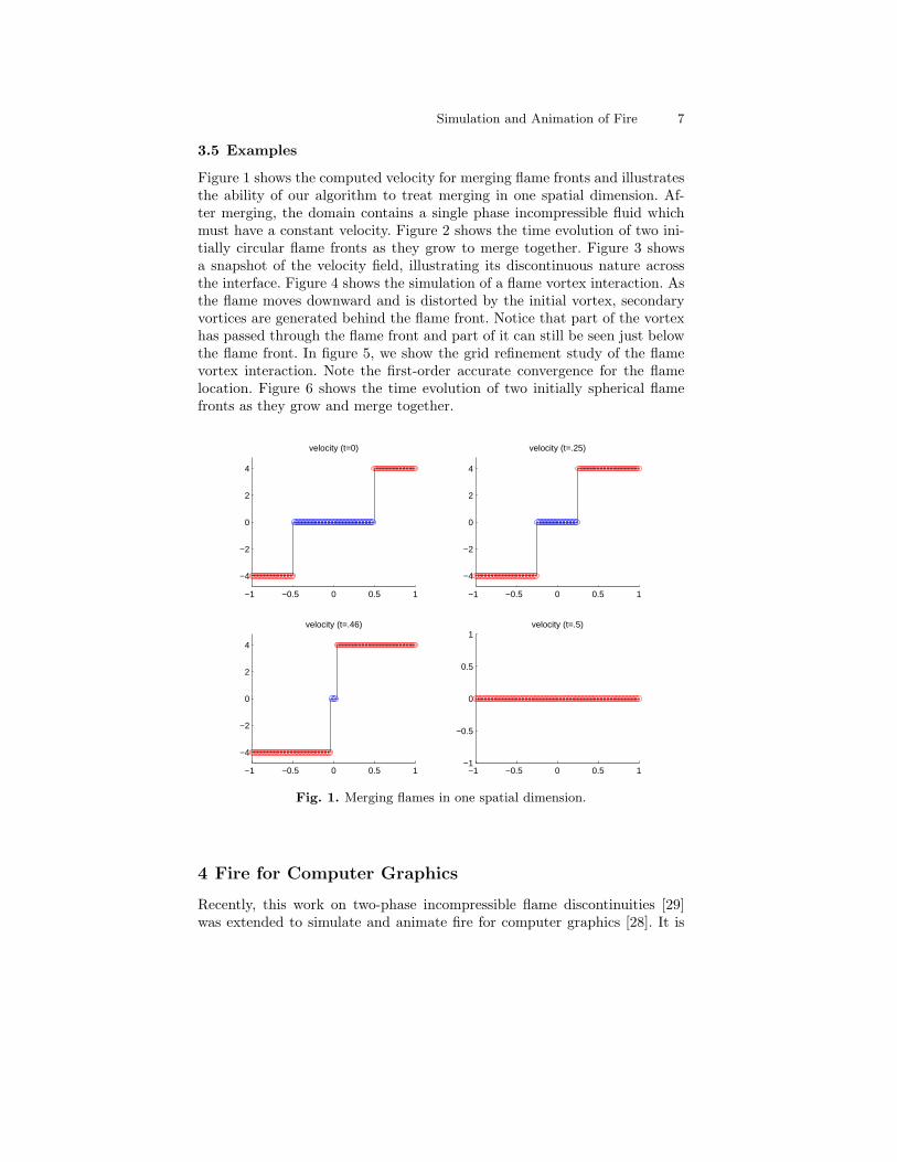
3.5 Examples

Figure 1 shows the computed velocity for merging flame fronts and illustratesthe ability of our algorithm to treat merging in one spatial dimension. Af-ter merging, the domain contains a single phase incompressible fluid whichmust have a constant velocity. Figure 2 shows the time evolution of two ini-tially circular flame fronts as they grow to merge together. Figure 3 showsa snapshot of the velocity field, illustrating its discontinuous nature acrossthe interface. Figure 4 shows the simulation of a flame vortex interaction. Asthe flame moves downward and is distorted by the initial vortex, secondaryvortices are generated behind the flame front. Notice that part of the vortexhas passed through the flame front and part of it can still be seen just belowthe flame front. In figure 5, we show the grid refinement study of the flamevortex interaction. Note the first-order accurate convergence for the flamelocation. Figure 6 shows the time evolution of two initially spherical flamefronts as they grow and merge together.

−1 −0.5 0 0.5 1

−4

−2

0

2

4

velocity (t=0)

−1 −0.5 0 0.5 1

−4

−2

0

2

4

velocity (t=.25)

−1 −0.5 0 0.5 1

−4

−2

0

2

4

velocity (t=.46)

−1 −0.5 0 0.5 1−1

−0.5

0

0.5

1velocity (t=.5)

Fig. 1. Merging flames in one spatial dimension.

4 Fire for Computer Graphics

Recently, this work on two-phase incompressible flame discontinuities [29]was extended to simulate and animate fire for computer graphics [28]. It is


0 0.5 1 1.50

0.1

0.2

0.3

0.4

0.5

0.6

0.7

0.8

0.9

1level set contour

t=0

t=.01

t=.02

t=.03

t=.04

t=.05

Fig. 2. Time evolution of two initially circular flame fronts as they grow to mergetogether.

0 0.5 1 1.50

0.1

0.2

0.3

0.4

0.5

0.6

0.7

0.8

0.9

1

velocity field (t=.05)

Fig. 3. Discontinuous velocity field depicted shortly after the two flame frontsmerge.

suitable for both smooth (laminar) and turbulent flames and it can be used toanimate the burning of both solid or gaseous fuels. The incompressible Eulerequations are used to independently model both the vaporized fuel and thehot gaseous products. A physically based model is used for the expansion thattakes place when a vaporized fuel reacts to form hot gaseous products, and arelated model is used for the similar expansion that takes place when a solidfuel is vaporized into a gaseous state. In addition to the hot gaseous products,smoke and soot rise under the influence of buoyancy and are rendered usinga blackbody radiation model. The method also models and renders the bluecore that results from the free radicals in the chemical reaction zone wherefuel is converted into products. The method also allows for the flame frontand smoke to interact with objects, with flammable objects able to catch onfire.

Buoyancy forces were added as body forcing terms to equation 1 to modelrising flames, i.e.

Vt + (V · ∇)V +∇p

ρ= f . (27)


0 1 2 3 4 54

5

6

7

8

9

10vorticity contour (t=1.5)

.5 .5

1.0

1.5 1.0

.5

−.5

−1.0

−1.5

−2.0

Fig. 4. Flame vortex interaction - secondary vorticity generation.

0 1 2 3 4 50

1

2

3

4

5

6

7

8

9

10level set contour

t=0

t=.5

t=1.0

t=1.5

t=2.0

t=2.5

t=3.0

t=3.5

Fig. 5. Flame vortex interaction - grid refinement.


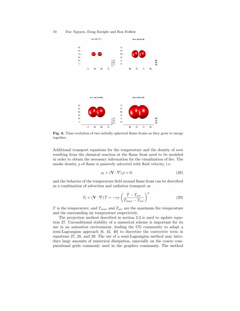
Fig. 6. Time evolution of two initially spherical flame fronts as they grow to mergetogether.

Additional transport equations for the temperature and the density of sootresulting from the chemical reaction at the flame front need to be modeledin order to obtain the necessary information for the visualization of fire. Thesmoke density ρ of flame is passively advected with fluid velocity, i.e.

ρt + (V · ∇) ρ = 0, (28)

and the behavior of the temperature field around flame front can be describedas a combination of advection and radiation transport as

Tt + (V · ∇) T = −cT

(T − Tair

Tmax − Tair

)4

. (29)

T is the temperature, and Tmax and Tair are the maximum fire temperatureand the surrounding air temperature respectively.

The projection method described in section 3.3 is used to update equa-tion 27. Unconditional stability of a numerical scheme is important for itsuse in an animation environment, leading the CG community to adopt asemi-Lagrangian approach [6, 42, 40] to discretize the convective term inequations 27, 28, and 29. The use of a semi-Lagrangian method may intro-duce large amounts of numerical dissipation, especially on the coarse com-putational grids commonly used in the graphics community. The method


of choice to reduce this dissipation is the “vorticity confinement” methodof Steinhoff [43]. This method was first introduced to the computer graph-ics community in [10]. The vorticity confinement body force adds additionalsmall scale rolling features characteristic of fire and smoke in a numericallyconsistent manner. This is accomplished by adding a swirling body forcein regions of the flow which posses large amounts of vorticity and are thussensitive to excessive amounts of artificial dissipation.

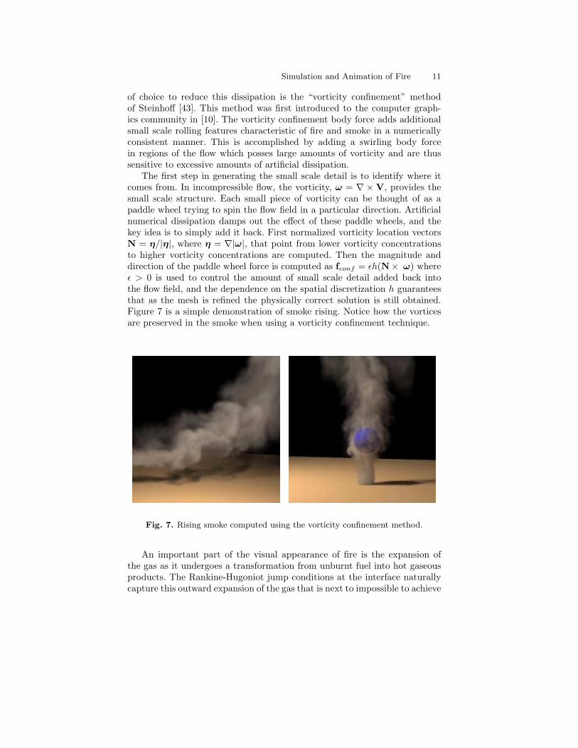
The first step in generating the small scale detail is to identify where itcomes from. In incompressible flow, the vorticity, ω = ∇ ×V, provides thesmall scale structure. Each small piece of vorticity can be thought of as apaddle wheel trying to spin the flow field in a particular direction. Artificialnumerical dissipation damps out the effect of these paddle wheels, and thekey idea is to simply add it back. First normalized vorticity location vectorsN = η/|η|, where η = ∇|ω|, that point from lower vorticity concentrationsto higher vorticity concentrations are computed. Then the magnitude anddirection of the paddle wheel force is computed as fconf = εh(N× ω) whereε > 0 is used to control the amount of small scale detail added back intothe flow field, and the dependence on the spatial discretization h guaranteesthat as the mesh is refined the physically correct solution is still obtained.Figure 7 is a simple demonstration of smoke rising. Notice how the vorticesare preserved in the smoke when using a vorticity confinement technique.

Fig. 7. Rising smoke computed using the vorticity confinement method.

An important part of the visual appearance of fire is the expansion ofthe gas as it undergoes a transformation from unburnt fuel into hot gaseousproducts. The Rankine-Hugoniot jump conditions at the interface naturallycapture this outward expansion of the gas that is next to impossible to achieve


using the low level hacks and random numbers usually resorted to by thecomputer graphics animation community.

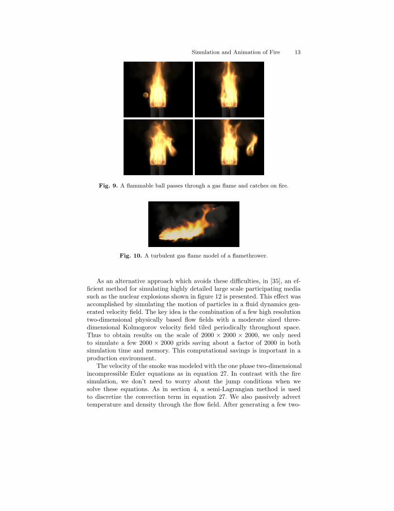
Figure 8 (left) shows two different blue cores with a differing flame speedS. The zero level set is used to represent this blue core with the unreactedgas inside the blue core. Figure 8 (right) shows three different flames withdifferent density ratios of unreacted and reacted gases. This density ratio in-creases from left to right, making the flame appear fuller and more turbulent.Figure 9 shows the ability of our model to interact with objects. In this ex-ample, a flammable ball flies through the fire and catches on fire. Figure 10illustrates the use of a turbulent flame model to simulate a flamethrower.Finally, figure 11 shows two burning logs that are placed on the ground andused to emit fuel. The crossways log on the top is not lit so the flame is forcedto flow around it.

Fig. 8. Blue reaction zone cores (left) and CG fire (right).

5 Smoke Simulation for Large Scale Phenomena

Large scale phenomena such as nuclear explosions are challenging to animaterealistically. For example, it is difficult to simulate the nuclear destructionof an entire city with the level of detail necessary for a feature film. More-over, reference video footage tends to be of low quality and resolution, socomputer simulations of these phenomena are preferable. The previously dis-cussed methods can produce near real time results on small grids and inter-active results on moderate sized grids. However, on very large grids of thescale 2000 × 2000 × 2000, these methods are impractical. In fact, a grid ofthis size would require about 120GB of memory just to store the density andvelocity field as floats (and twice that much for doubles), which is well beyondthe capability of a high end workstation. Besides these storage limitations,a fully three dimensional compressible flow simulation of this phenomenonis not suitable for use in a production environment due to the small timestep requirement resulting from the large sound speed in the compressibleequations.


Fig. 9. A flammable ball passes through a gas flame and catches on fire.

Fig. 10. A turbulent gas flame model of a flamethrower.

As an alternative approach which avoids these difficulties, in [35], an ef-ficient method for simulating highly detailed large scale participating mediasuch as the nuclear explosions shown in figure 12 is presented. This effect wasaccomplished by simulating the motion of particles in a fluid dynamics gen-erated velocity field. The key idea is the combination of a few high resolutiontwo-dimensional physically based flow fields with a moderate sized three-dimensional Kolmogorov velocity field tiled periodically throughout space.Thus to obtain results on the scale of 2000 × 2000 × 2000, we only needto simulate a few 2000 × 2000 grids saving about a factor of 2000 in bothsimulation time and memory. This computational savings is important in aproduction environment.

The velocity of the smoke was modeled with the one phase two-dimensionalincompressible Euler equations as in equation 27. In contrast with the firesimulation, we don’t need to worry about the jump conditions when wesolve these equations. As in section 4, a semi-Lagrangian method is usedto discretize the convection term in equation 27. We also passively advecttemperature and density through the flow field. After generating a few two-


Fig. 11. A CG campfire.

dimensional velocity fields, we define a three-dimensional velocity field viainterpolation. Parallel and cylindrical interpolations give nice results, how-ever the method is not limited to these two interpolation schemes.

Since we build a three-dimensional velocity field from multiple two-dimensional solutions of Euler equations, it is desirable to add a fully three-dimensional component to the velocity field. This is accomplished using aKolmogorov spectrum which is described in detail in [41] and used in manyapplications, e.g. to model fire in [24]. The main idea is to use random num-bers to construct an energy spectrum in Fourier space that subsequentlydetermines the structure of the velocity field. After constructing an energyspectrum in Fourier space, one enforces the divergence free condition and usesan inverse FFT to obtain a velocity field full of small scale eddies. Since thevelocity field is periodic, a single grid can be used as a tiling of all of space.Moreover, one can use two grids of different sizes to increase the period ofrepetition to the least common multiple of their lengths alleviating visuallytroublesome spatial repetition (although this is a minor point for us since weblend the Kolmogorov velocity field with the non-periodic CFD/interpolationgenerated velocity field). We also fill the time domain by constructing a fewKolmogorov velocity fields, assigning each one to a different point in time,and interpolating between them at intermediate times. In practice, two spec-trums are usually enough and we alternate between them every 24 frames (24frames equals one second for film). Finally, at any point in space and time,we define the total velocity field as a linear combination of the Kolmogorov


Fig. 12. A CG Nuclear Explosion.

velocity field and the CFD/interpolation generated velocity field. Again, westress that we do not use this to construct a three-dimensional velocity field,but instead compute the velocity at a point in space and time on the fly usingthe Kolmogorov velocity field, the two-dimensional CFD generated velocityfields, and chosen interpolation rules.

Once we have implicitly defined our flow field at every point of interestin space and time, we can passively advect particles through the flow usingxt = u where x is the particle position for the rendering purpose. The par-ticle attributes include temperature, density of smoke, velocity and position.If desired, copies of two-dimensional flow fields and the three-dimensionalKolmogorov velocity field can be distributed to multiple processors whereparticles can be passively evolved with no intercommunication requirements.This allows one to generate an incredibly large numbers of particles, althoughwe have found that even one processor can readily generate enough particlesto move the bottleneck to the rendering stage.

6 Alternative Techniques

Particle-based techniques have been quite popular for the animation of fire.Starting with the early use of a particle system for a visual effects shot inthe Genesis sequence in “Star Trek II: The Wrath of Khan” [36], particle sys-tems continue to provide a simple, yet quite effective way to model “fuzzy”


natural phenomena, including smoke and fire. We briefly review two recentlyproposed particle-based methods to model fire for computer graphics pur-poses. Feldman et al. [14] coupled a particle system with an appropriatelymodified one-phase Navier-Stokes solver for the purpose of animating sus-pended particle explosions. Lamorlette and Foster [24], focused on developinga method which provides a great degree of user control over the flame behav-ior, including imposing non-physically based behavior, while still preservingthe essentially “chaotic” nature of fire.

In [14], the authors used a one phase incompressible fluid model. However,instead of using a divergence free condition for incompressible flow, the typicaldivergence free condition was modified to model the expansion of gas aftera chemical reaction happens. Particles are used to keep track of the motionof particulate fuel and soot, and interact with the underlying fluid systemthrough the transfer of momentum and heat.

Specifically, a single phase three-dimensional incompressible Euler equa-tion (as in equation 27) is used to model the hot gas and products combined.The divergence free condition is modified as

∇ ·V = φ (30)

where φ is zero except where the detonation process and subsequent expan-sion is taking place. In order to enforce equation 30, a modified version ofequation 19 is solved, i.e.

4p? = ρ (∇ ·V? − φ) , (31)

to determine the pressure field. Note that the density is spatially constant andhas been moved to the right hand side. The fluid temperature is described as

Tt + (V · ∇) T = −cr

(T − Ta

Tmax − Ta

)4

+ ck∇2T +1

ρcvHt (32)

where Ta is the ambient temperature, and H is the heat energy transferredto the fluid from the reacting particles.

A particle model is used to represent the fuel and solid combustion prod-ucts (i.e. soot). A particle possesses attributes including its position, velocity,mass, temperature, thermal mass, volume, and type. The particle is governedby

xtt =fm

and Yt =Ht

cm, (33)

where x denotes the location of the particle, H is the heat energy transferredto the particle or generated by combustion, Y is the particle temperature,and cm is the particle’s thermal mass.

The underlying fluid and the particles interact through the transfer ofmomentum and heat energy. When the particle moves through the fluid,a constant coefficient drag force law is imposed. This force is given by


f = αdr2(u − xt) ‖ u − xt ‖, where αd is the drag coefficient, r is the

particle radius, and u is the fluid velocity interpolated to the location of theparticle. Similarly, Ht = αhr2(T − Y ) governs the thermal transfer betweenthe particles and the fluid. A fuel particle will ignite when its temperaturerises above an ignition point. The burning particles generate heat at the rateHt = bhz, where bh denotes the amount of heat released per unit combustedmass of the fuel and z is the burning rate. While a particle is burning, thegaseous products produced from the combustion process are accounted for inthe fluid by modifying the φ value of the cell in which the particle resides,i.e. ∆φ = 1

V bgz, where V is the volume of the cell and bg denotes the volumeof gas released per unit combusted mass less the volume of gas consumed.

While this technique is effective in providing a physically plausible modelto capture the visual after-effects of an explosive process while avoiding thenumerical difficulties and small time steps associated with a fully featuredgrid-based compressible flow model [49], the flame (explosion) is discretelydefined by particles resulting in a spatially incoherent front. In the case ofexploding fireballs, the lack of a spatially coherent interface is visually accept-able, but as indicated by the authors in [14], their method has difficulty indealing with flame fronts with a higher degree of spatial structure such as seenin burning liquid fuels. The use of a spatially coherent interface technique,e.g. a level set method, avoids this visually disturbing feature as illustratedby the simulation of a flamethrower using the method of Nguyen et al. infigure 10.

Lamorlette and Foster [24] noted that fire can be used in feature filmsas a dramatic element, thus requiring the maximum level of control while atthe same time maintaining a believable appearance. An example of the use offire in this manner is the stylized fire-breathing dragon in the movie “Shrek”.To provide the degree of control required to model fire-breathing dragons,Lamorlette and Foster proposed a particle-based fire animation tool utiliz-ing many of the classical computer graphics techniques for simulating naturalphenomena, including stochastic methods, procedural noise, Kolmogorov tur-bulent noise, artificial wind fields, and flame control curves.

In [24], the basic structural element of the flame is given by particlesconnected together into an interpolating B-spline curve. The particles areaffected by arbitrary wind fields, Brownian diffusion, the motion of the firesource (with velocity Vp), and thermal buoyancy. After defining these variousflame behaviors, the motion of a given interpolating particle with temperatureTp is given by

dxp

dt= w(xp, t) + d(Tp) + Vp + c(Tp, t; tp), (34)

where w(xp, t) is the controlling wind field, d(Tp) is the amount of randomBrownian motion modeling diffusive processes, and c(Tp, t; tp) represents thethermal buoyancy with tp indicating a functional dependence on the overalllifetime of the particle. To avoid modeling a temperature field over the entire


domain, the thermal buoyancy is made to depend upon the lifetime of theparticle, i.e. c(Tp, t; tp) = −βg(To − Tp)t2p, with To the ambient temperatureand β the coefficient of thermal expansion. An explicit Runge-Kutta methodis used to advance equation 34 in time. The spline is resampled after eachtime step with the particles redistributed to ensure no aliasing features arepresent. Individual flame strands are allowed to pinch off after reaching a setlength at a rate given by a statistical model. The size of the separated flameis determined according to a normal distribution. An ad hoc estimate of theamount of fuel left in a separated flame is made in order to control how longit remains visible.

To provide visual fullness, a model of the actual visible flame region is nec-essary. A volumetric model is used, with the volume defined by a shape offsetvolume-of-revolution technique. A simple, two-dimensional profile is chosenfrom a library of shapes and rotated about the B-spline based particle back-bone of the flame. A volumetric 1/r2 light density function motivated bythe combustion process actually occurring at the flame front is then definedaccording to the position of the swept out parametric surface. This densityfunction is statistically point sampled to easily allow for additional deforma-tion and noise fields to be added. To provide for additional detail which ismissing from the simple volumetric flame model discussed above, two levelsof structural noise are added to the model. The first models fluctuations inthe combustion process at the base of the flame. These fluctuations propagateup the structural backbone of the flame, causing the volumetrically sampledpoints to be displaced. Perlin’s flow noise model [32] is used to determine thesize of the fluctuations. For a finer, more turbulence driven perturbation ofthe sample points, Kolmogorov noise is added. The volumetric description ofthe flame readily allows for merging of neighboring flames, as in the level setmethod. After performing all of these operations, the particles are rendered.The color of each volumetric flame particle is not physically based, ratherit is taken from a reference photograph texture mapped to the swept outtwo-dimensional library profile. The intensity of the light is based upon the1/r2 falloff light density function previously discussed. This entire procedureis repeated each time step, with no frame-to-frame coherency informationretained. For further details about this technique, the reader is referred tothe original paper [24]. Overall, this method for flame animation allows fora much finer degree of control than a purely physics-based model at the costof sacrificing the ability to procedurally capture many of the subtle effectswhich visually define fire.

7 A Few Comments on Water

In contrast to the modeling and simulation of the physically complex phenom-ena which describe low speed flame propagation, the tracking of a passivelyadvected interface between two liquid phases, e.g. air and water, is almost


simple by comparison. However, unlike fire which is visually defined by thevolume of soot and the hot gaseous products produced during the combus-tion process, the defining characteristic of water is the thin, smooth contactdiscontinuity between the water and air. This fact places a host of stringentrequirements on any method used to represent this interface, i.e. the methodneeds to: accurately track the underlying flow characteristics, readily allowfor changes in the topology of the interface (pinching and merging), be com-putationally tractable, and not suffer from excessive amounts of numericaldiffusion while maintaining a spatially and temporally smooth interface.

Lagrangian based interface techniques [19, 45] partially satisfy some ofthese requirements, exhibiting an excellent ability to track underlying flowcharacteristics without significant amounts of numerical diffusion. However,the use of a discrete, marker particle based method to represent the fluid doesnot readily allow for a visually smooth interface to be reconstructed from thefluid particles. Moreover, a connected marker particle approach requires theuse of complex remeshing algorithms to deal with topological changes.

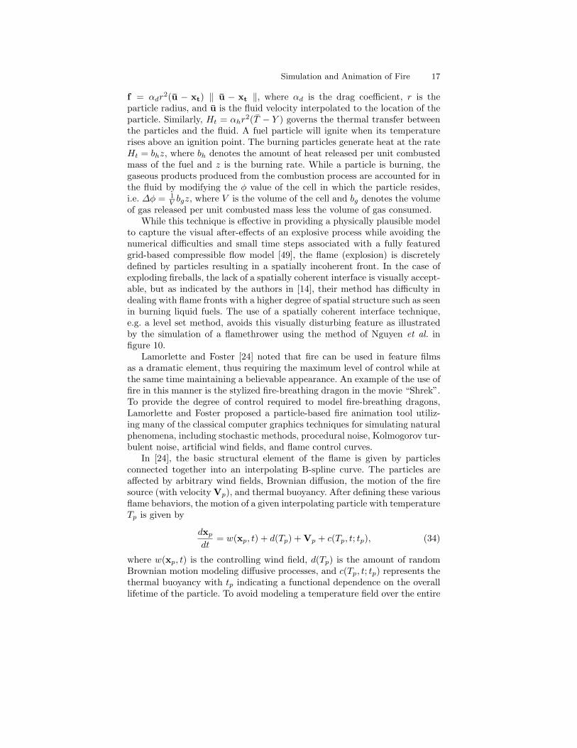
Eulerian based methods, e.g. Volume of Fluid (VOF) [21, 37] and level setmethods [31], readily allow for topological changes due to the underlying gridrepresentation used. However, these schemes are all subject to large amountsof mass loss and can be computationally expensive due to the embedding ofthe lower-dimensional interface in a higher-dimensional grid. VOF schemesattempt to cure the mass loss problem by imposing an artifical mass con-servation constraint. In VOF schemes, regions of high curvature and thin,filamentary regions of the interface have difficulty in accurately sampling theunderlying flow field, causing small pieces of “flotsam” and “jetsam” to formand move in visually unnatural ways. Alternatively, level set methods canmaintain a smooth interface due to the signed distance property of the levelset function. High order accurate HJ-WENO schemes [38] along with periodicreinitialization [44] can alleviate the diffusion of large scale interface features,but numerical dissipation makes it difficult to maintain small scale features.An example of the adverse effects of numerical dissipation can be seen infigure 13, where the notched disk in figure 13(a) undergoes a rigid body ro-tation. After one rotation of the disk the level set function has experiencedan excessive amount of nonphysical diffusion in the corners and throughoutthe thin notch as seen in figure 13(b). A recently proposed interface captur-ing technique, the particle level set method [7], combines the strengths ofLagrangian and Eulerian methods.

The interface in the particle level set method is represented as the zero iso-contour of a signed distance function φ. Massless marker particles are placedin a band about the interface to act as a diffusion control mechanism. The re-sults of the particle level set method can be seen in figure 13(c) where the thinnotch along with the sharp corners have maintained their original shape withlittle to no diffusion. The particles move according to dxp/dt = V(xp), andeach particle possesses a radius rp and a sign sp. Since the level set is tracking


30 35 40 45 50 55 60 65 7055

60

65

70

75

80

85

90

95

x

y

(a) Initial

30 35 40 45 50 55 60 65 7055

60

65

70

75

80

85

90

95

x

y

(b) Level Set Only

30 35 40 45 50 55 60 65 7055

60

65

70

75

80

85

90

95

x

y

(c) Particle Level Set

Fig. 13. Rigid body rotation of a notched disk.

a contact discontinuity, particles which correspond to the φ > 0 region shouldalways remain in the φ > 0 region and vice versa, however excessive amountsof numerical diffusion can cause positive particles, i.e. particles with sp = +1,to end up in a φ < 0 region according to the level set function. These parti-cles are said to have “escaped” from their respective side of the interface andindicate that a first order error in the location of the interface has occurred.This first order accurate error in φ can be corrected for by the particles sincethe radius of each particle defines a local level set function, φp, which wecan compare against φ at the corners of the grid cell containing the particle.After iterating through all the escaped particles and determining corrected φvalues, the particles then resample their distance to the interface and adjusttheir radii accordingly. This error reduction technique can also be used tocorrect errors made when φ is reinitialized to be a signed distance function.In this case the particle velocity is assumed to be zero since the interfaceshould not move. A complete description of this error reduction techniquecan be found in [7].

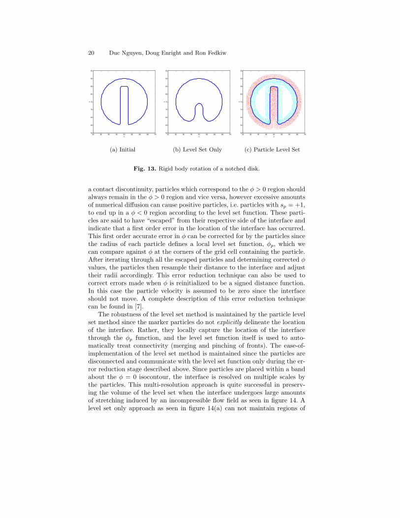
The robustness of the level set method is maintained by the particle levelset method since the marker particles do not explicitly delineate the locationof the interface. Rather, they locally capture the location of the interfacethrough the φp function, and the level set function itself is used to auto-matically treat connectivity (merging and pinching of fronts). The ease-of-implementation of the level set method is maintained since the particles aredisconnected and communicate with the level set function only during the er-ror reduction stage described above. Since particles are placed within a bandabout the φ = 0 isocontour, the interface is resolved on multiple scales bythe particles. This multi-resolution approach is quite successful in preserv-ing the volume of the level set when the interface undergoes large amountsof stretching induced by an incompressible flow field as seen in figure 14. Alevel set only approach as seen in figure 14(a) can not maintain regions of


��

(a) Level Set Only

��

(b) Particle Level Set

Fig. 14. 3D deformation test.

high curvature and the thin (approximately one grid cell thick) pancake re-gion formed during the deformation process. On the other hand, the particlelevel set method can resolve these regions on the 1003 grid used. Also, whiletearing of the interface is seen in the thin pancake region with the particlelevel set method, particles which remain escaped are not deleted and cancontribute to the rebuilding of the interface as seen in the last row of framesin figure 14(b). The sphere, which loses over 80% of its volume by the endof the deformation process when represented with a level set only method,loses only 2% of its volume with the particle level set method. The addi-tional cost of placing particles near the interface is offset by the ability touse much coarser volumetric grids when calculating the pressure during flowcalculations without sacrificing a faithful representation of the interface.

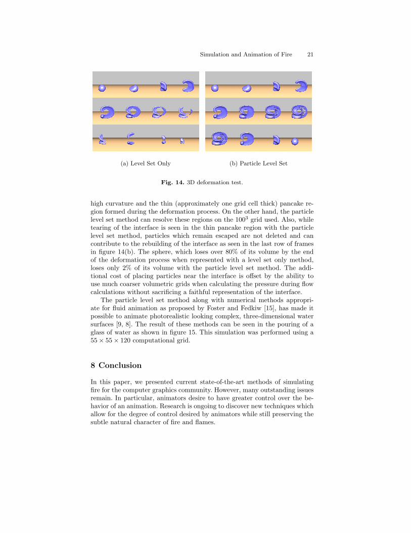
The particle level set method along with numerical methods appropri-ate for fluid animation as proposed by Foster and Fedkiw [15], has made itpossible to animate photorealistic looking complex, three-dimensional watersurfaces [9, 8]. The result of these methods can be seen in the pouring of aglass of water as shown in figure 15. This simulation was performed using a55× 55× 120 computational grid.

8 Conclusion

In this paper, we presented current state-of-the-art methods of simulatingfire for the computer graphics community. However, many outstanding issuesremain. In particular, animators desire to have greater control over the be-havior of an animation. Research is ongoing to discover new techniques whichallow for the degree of control desired by animators while still preserving thesubtle natural character of fire and flames.


Fig. 15. Pouring of a glass of water.

9 Acknowledgments

Research supported in part by an ONR YIP and PECASE award (ONRN00014-01-1-0620), a Packard Foundation Fellowship, a Sloan Research Fel-lowship, ONR N00014-03-1-0071, NSF DMS-0106694 and NSF ITR-0121288.In addition, D.E. was supported in part by an NSF postdoctoral fellowship(NSF DMS-0202459).

References

1. Adalsteinsson, D. and Sethian, J., A Fast Level Set Method for PropagatingInterfaces, J. Comp. Phys. 118, 269–277 (1995).

2. Brackbill, J., Kothe, D. and Zemach, C., A Continuum Method for ModelingSurface Tension, J. Comp. Phys. 100, 335–354 (1992).

3. Caiden, R., Fedkiw, R. and Anderson, C., A Numerical Method For Two-Phase Flow Consisting of Separate Compressible and Incompressible Regions ,J. Comp. Phys. 166, 1–27 (2001).

4. Chen, S., Merriman, B., Kang, M., Caflisch, R., Ratsch, C., Cheng, L.-T.,Gyure, M., Fedkiw, R., Anderson, C. and Osher, S., Level Set Method for ThinFilm Epitaxial Growth, J. Comp. Phys. 167, 475–500 (2001).

5. Chorin, A. J., Numerical Solution of the Navier-Stokes Equations , Math. Comp.22, 745–762 (1968).

6. Courant, R., Issacson, E. and Rees, M., On the Solution of Nonlinear HyperbolicDifferential Equations by Finite Differences , Comm. Pure and Applied Math5, 243–255 (1952).

7. Enright, D., Fedkiw, R., Ferziger, J. and Mitchell, I., A Hybrid Particle LevelSet Method for Improved Interface Capturing , J. Comp. Phys. 183, 83–116(2002).

8. Enright, D., Marschner, S. and Fedkiw, R., Animation and Rendering of Com-plex Water Surfaces, ACM Trans. on Graphics (SIGGRAPH 2002 Proceedings)21, 736–744 (2002).


9. Enright, D., Nguyen, D., Gibou, F. and Fedkiw, R., Using the Particle Level SetMethod and a Second Order Accurate Pressure Boundary Condition for FreeSurface Flows, in Kawahashi, M., Ogut, A. and Tsuji, Y., eds., Proceedingsof the 4th ASME-JSME Joint Fluids Engineering Conference , FEDSM2003–45144, ASME, 2003.

10. Fedkiw, R., Stam, J. and Jensen, H. W., Visual Simulation of Smoke, in Fiume,E., ed., Proceedings of SIGGRAPH 2001 , Computer Graphics Proceedings,Annual Conference Series, pp. 15–22, ACM, ACM Press / ACM SIGGRAPH,2001.

11. Fedkiw, R. P., Coupling an Eulerian Fluid Calculation to a Lagrangian SolidCalculation with the Ghost Fluid Method , J. Comp. Phys. 175, 200–224 (2002).

12. Fedkiw, R. P., Aslam, T., Merriman, B. and Osher, S., A Non-oscillatory Eule-rian Approach to Interfaces in Multimaterial Flows (The Ghost Fluid Method),J. Comp. Phys. 152, 457–492 (1999).

13. Fedkiw, R. P., Aslam, T. and Xu, S., The Ghost Fluid Method for Deflagrationand Detonation Discontinuities , J. Comp. Phys. 154, 393–427 (1999).

14. Feldman, B. E., O’Brien, J. F. and Arikan, O., Animating Suspended ParticleExplosions, ACM Transactions on Graphics 22, 708–715 (2003).

15. Foster, N. and Fedkiw, R., Practical Animation of Liquids , in Fiume, E., ed.,Proceedings of SIGGRAPH 2001 , Computer Graphics Proceedings, AnnualConference Series, pp. 23–30, ACM, ACM Press / ACM SIGGRAPH, 2001.

16. Foster, N. and Metaxas, D., Modeling the Motion of a Hot, Turbulent Gas ,in Proceedings of SIGGRAPH 1997 , Computer Graphics Proceedings, AnnualConference Series, pp. 181–188, ACM, ACM Press / ACM SIGGRAPH, 1997.

17. Gibou, F., Fedkiw, R., Caflisch, R. and Osher, S., A Level Set Approach forthe Numerical Simulation of Dendritic Growth , J. Sci. Comput. 19, 183–199(2003).

18. Gibou, F., Fedkiw, R. P., Cheng, L.-T. and Kang, M., A Second–Order–Accurate Symmetric Discretization of the Poisson Equation on Irregular Do-mains, J. Comp. Phys. 176, 205–227 (2002).

19. Harlow, F. and Welch, J., Numerical Calculation of Time-Dependent ViscousIncompressible Flow of Fluid with Free Surface, Phys. Fluids 8, 2182–2189(1965).

20. Helenbrook, B. and Law, C., A numerical Method for Solving InocmpressilbeFlow Problems with a Surface of Discontinuity , J. Comp. Phys. 148, 366–396(1999).

21. Hirt, C. and Nichols, B., Volume of Fluid (VOF) Method for the Dynamics ofFree Boundaries, J. Comp. Phys. 39, 201–225 (1981).

22. Juric, D. and Tryggvason, G., Computations of Boiling Flows , J. Comp. Phys.24, 387–410 (1998).

23. Kang, M., Fedkiw, R. and Liu, X.-D., A Boundary Condition Capturing Methodfor Multiphase Incompressible Flow , J. Sci. Comput. 15, 323–360 (2000).

24. Lamorlette, A. and Foster, N., Structural Modeling of Natural Flames , ACMTransactions on Graphics 21, 729–735 (2002).

25. Liu, X.-D., Fedkiw, R. and Kang, M., A Boundary Condition Capturing Methodfor Poisson’s Equation on Irregular Domains , J. Comp. Phys. 160, 151–178(2000).

26. Neff, M. and Fiume, E., A Visual Model for Blast Waves and Fracture, in Pro-ceedings of SIGGRAPH 1999 , Computer Graphics Proceedings, Annual Con-ference Series, pp. 193–202, ACM, ACM Press / ACM SIGGRAPH, 1999.


27. Nguyen, D., Gibou, F. and Fedkiw, R., A Fully Conservative Ghost FluidMethod and Stiff Detonation Waves , in 12th International Detonation Sym-posium, ONR, 2002.

28. Nguyen, D. Q., Fedkiw, R. and Jensen, H. W., Physically Based Modeling andAnimation of Fire, ACM Trans. on Graphics (SIGGRAPH 2002 Proceedings)21, 721–728 (2002).

29. Nguyen, D. Q., Fedkiw, R. P. and Kang, M., A Boundary Condition CapturingMethod for Incompressible Flame Discontinuities , J. Comp. Phys. 172, 71–98(2001).

30. Osher, S. and Fedkiw, R., Level Set Methods and Dynamic Implicit Surfaces ,Springer-Verlag, New York, 2002.

31. Osher, S. and Sethian, J., Fronts Propagating with Curvature Dependent Speed:Algorithms Based On Hamiliton-Jacobi Formulations , J. Comp. Phys. 79, 12–49 (1988).

32. Perlin, K. and Neyret, F., Flow Noise, in SIGGRAPH Technical Sketches andApplications, ACM, 2001.

33. Peskin, C., Numerical Analysis of Blood flow in the Heart , J. Comp. Phys. 25,220–252 (1977).

34. Quian, J., Tryggvason, G. and Law, C., A Front Method for the Motion ofPremixed Flames, J. Comp. Phys. 144, 52–69 (1998).

35. Rasmussen, N., Nguyen, D., Geiger, W. and Fedkiw, R., Smoke SimulationFor Large Scale Phenomena, in Proceedings of SIGGRAPH 2003 , ComputerGraphics Proceedings, Annual Conference Series, pp. 703–707, ACM, ACMPress / ACM SIGGRAPH, 2003.

36. Reeves, W., Particle Systems - A Technique for Modeling a Class of FuzzyObjects, in Computer Graphics (Proceedings of SIGGRAPH 83), volume 17,pp. 359–376, ACM, 1983.

37. Rider, W. and Kothe, D., Reconstructing Volume Tracking , J. Comp. Phys.141, 112–152 (1998).

38. Shu, C. and Osher, S., Efficient Implementation of Essentially Non-OscillatoryShock Capturing Schemes , J. Comp. Phys. 77, 439–471 (1988).

39. Son, G. and Dir, V., Numerical Simulation of Film Boiling near Critical Pres-sures with a Level Set Method , J. Heat Transfer 120, 183–192 (1998).

40. Stam, J., Stable Fluids, in Proceedings of SIGGRAPH 99 , Computer GraphicsProceedings, Annual Conference Series, pp. 121–128, ACM, ACM SIGGRAPH/ Addison Wesley Longman, 1999.

41. Stam, J. and Fiume, E., Turbulent Wind Fields for Gaseous Phenomena , inProceedings of SIGGRAPH 1993 , Computer Graphics Proceedings, AnnualConference Series, pp. 369–376, ACM, ACM Press / ACM SIGGRAPH, 1993.

42. Staniforth, A. and Cote, J., Semi-Lagrangian Integration Schemes for Atmo-spheric Models - A Review , Monthly Weather Review 119, 2206–2223 (1991).

43. Steinhoff, J. and Underhill, D., Modification of the Euler Equations for ”vor-ticity confinement”: Application to the computation of interacting vortex rings ,Phys. Fluids 6, 2738–2744 (1994).

44. Sussman, M., Smereka, P. and Osher, S., A Level Set Approach for ComputingSolutions to Incompressible Two-Phase Flow , J. Comp. Phys. 114, 146–159(1994).

45. Tryggvason, G., Bunner, B., Esmaeeli, A., Juric, D., Al-Rawahi, N., Tauber, W.,Han, J., Nas, S. and Jan, Y.-J., A Front-Tracking Method for the Computationsof Multiphase Flow , J. Comp. Phys. 169, 708–759 (2001).


46. Unverdi, S. and Tryggvason, G., A Front-Tracking Method for Vicous, Incom-pressible, Multi-Fluid Flows , J. Comp. Phys. 100, 25–37 (1992).

47. Welch, S. and Wilson, J., A Volume of Fluid Based Method for Fluid Flowswith Phase Change, J. Comp. Phys. 160, 662–682 (2000).

48. Yngve, G. and O’Brien, J., Animating Explosions , in Proceedings of SIG-GRAPH 2000 , Computer Graphics Proceedings, Annual Conference Series, pp.29–36, ACM, ACM Press / ACM SIGGRAPH, 2000.

49. Yngve, G. D., O’Brien, J. F. and Hodgins, J. K., Animating Explosions, in Pro-ceedings of ACM SIGGRAPH 2000 , Computer Graphics Proceedings, AnnualConference Series, pp. 29–36, 2000.

50. Zhang, Y., Yeo, K., Khoo, B. and Wang, C., 3D Jet Impact and Toroidal Bub-bles, J. Comp. Phys. 166, 336–360 (2001).

Documents

Simulation and Animation of Fire and Other Natural ...physbam.stanford.edu/~fedkiw/papers/stanford2003-11.pdf · Simulation and Animation of Fire and Other Natural Phenomena in the