Embed Size (px)
Citation preview
Simulation and Analysis of LEACH for Wireless Sensor
Networks in Agriculture
Latifah Munirah Kamarudin
*, R. Badlishah Ahmad
School of Computer and Communication Engineering,
Universiti Malaysia Perlis (UniMAP),
02600, Malaysia
Email: [email protected]
Email: [email protected]
*Corresponding author
David L. Ndzi
School of Engineering,
University of Portsmouth,
Portsmouth, PO1 3DJ, UK
Email: [email protected]
Ammar Zakaria, Kamarulzaman Kamarudin
Centre of Excellence for Advanced Sensor Technology
Universiti Malaysia Perlis
02600, Malaysia
E-mail: [email protected]
Email: [email protected]
Mohamed Elshaikh Elobaid Said Ahmed
School of Computer and Communication Engineering,
Universiti Malaysia Perlis (UniMAP),
02600, Malaysia
Email: [email protected]
Abstract: The challenges in deploying robust Wireless Sensor Networks (WSNs) in
agricultural environments are limited power supply and variability of wireless propagation
channel that restrict performance. Proposed protocols do not meet the challenges for
realistic simulation and evaluation of WSN for agricultural applications. The design of
LEACH protocol is, for the most part, efficient for many applications. It achieves energy
efficiency through a clustering technique with TDMA based MAC layer algorithms and
data aggregation method. Analysis performed shows that LEACH uses simple radio
propagation and energy models that are unrealistic. This paper focuses on the performance
analysis of LEACH protocol for agricultural environments.
Keywords: wireless sensor networks; LEACH; vegetation propagation model; clustering
protocol; MAC layer protocol, internet of things
Reference to this paper should be made as follows:
2
Latifah Munirah Kamarudin
Biographical notes: Latifah Munirah Kamarudin received her Ph.D from Universiti Malaysia
Perlis and her MSc from University of Porstmouth. She is a professional member of British
Computer Society. Her research interests include wireless sensor network, internet of things,
radio propagation modelling, wireless communication and network.
R. Badlishah Ahmad
Biographical notes: R. Badlishah Ahmad obtained his Ph.D and MSc from University of
Strathclyde. His research interests are in computer and telecommunication network modeling
using discrete event simulators (OMNeT++), optical networking and embedded system based on
GNU/Linux.
David L. Ndzi
Biographical notes: David L. Ndzi graduated with a PhD from University of Portsmouth. His
research covers wideband and narrow band wireless communication, channel characterization,
channel estimation and wireless sensor networks.
Ammar Zakaria
Biographical notes: Ammar Zakaria obtained his Ph.D from University Malaysia Perlis. His
research interests include data fusion, Intelligence sensing system and Bio-inspired sensor
system.
Kamarulzaman Kamarudin is a Ph.D. student at the CEASTech, Universiti Malaysia Perlis in the
field of Mechatronics and Robotics. He obtained B.Eng. in Mechatronics Engineering from
University of Canterbury, New Zealand. His main research interests are mobile robot olfaction,
image processing, sensors technologies and wireless sensor network (WSN).
Mohamed Elshaikh Elobaid Said Ahmed
Biographical notes: Mohamed Elshaikh received his MSc. from University Technology Petronas
(Malaysia), and currently pursuing his Ph.D at University Malaysia Perlis. He is also a
professional member at British Computer Society. His research interest includes Wireless
Network Protocols, network modeling and simulation, and internet of things.
1. Introduction
Wireless Sensor Networks (WSNs) have emerged as the next wave of wireless technology
particularly in internet of things (IoT), allowing unbounded physical environment to be
monitored and control. A WSN consists of spatially distributed sensory devices that are small in
size and able to sense, process data, and communicate with each other wirelessly. Networks of
hundreds to thousands of the sensor nodes are envisioned to allow monitoring of a wide variety
of phenomena with outstanding quality and scale. WSNs applications range from medical care
3
[1], environmental monitoring, such as early disaster warning [1-4], to precision agriculture [5-
7]. Recently, there has been a significant expansion of land use for plantations such as oil palm
[8], rubber and other commercially cultivated crops such as mangoes, which requires WSNs as
the enabling technology to improve post harvest production, quality assessment, control crop
growing conditions and automate agricultural process[9,10].
The technological challenges for developing and deploying WSNs in agriculture are
daunting. Applications in agriculture usually involve wide area monitoring, in the absence of
electrical power supply, harsh microclimate where degradable wireless links are unavoidable.
Wireless signal propagating inagricultural environments such as in oil palm plantations are
subject to many propagation losses due to blockage by trunks and/or shadowing in a hilly terrain,
diffraction losses and scattering by trees which lead to reduced communication range and packet
losses due to channel temporal variability.Thus, the application of WSN in agriculture needs to
be carefully planned in terms of sensor nodes placements, network topology and communication
protocols to ensure the system durable under a range of environmental stresses, including short
and long term degradation due to weather conditions. WSNs systems are expected to provide
continuous monitoring for long periods of time. Furthermore, network topology should be
carefully designed to avoid data losses due to lost connectivity between nodes, since the typical
propagation environment is characterized by the presence of trees, rocks and hills, which
attenuates radio waves. Depending on the application, data from the sensor nodes are sent to the
base station at seconds, minutes or hourly intervals or triggered by events [11,12]. To conserve
energy for longer network lifetime, a suitable protocol is needed at MAC level to provide
effective sleep and wake up patterns. The percentage of time each node is awake is known as the
node’s duty cycle, and a variety of approaches are available for achieving low duty-cycle
operation. The routing protocol implemented is another important consideration since the area is
large with densely deployed nodes. Therefore, the routing protocol used must be energy efficient
to deliver data from the nodes to the base station.
Several research studies in WSN have proposed various algorithms and protocols [13].
Their main aim is to optimize energy consumption and prolong network lifetime since in some
applications battery replacement can be difficult and node failure can be costly. Clustering
technique has been proven to be energy efficient and scalable [14]. Various cluster based routing
protocols have been proposed for WSNs in the past few years. Although many of them produced
results in some form of energy efficient clusters, only a few carefully considered the target
4
applications scenarios such as the effects of different physical propagation mechanisms in the
environment when forming clusters.
Low Energy Adaptive Clustering Hierarchy (LEACH) proposed by Heinzelman et al.
[14] is a well-known clustering protocol for WSNs that has been used widely in the literatures.
LEACH has attracted intensive attention because of its energy efficiency, simplicity and load
balancing properties. LEACH combines the cluster-based routing and MAC-layer techniques
along with application specific data aggregation to prolong network lifetime. In LEACH, cluster
head role is rotated among the nodes to prevent energy draining of a single node. There is
another variation of LEACH, which is named as LEACH-C. In this scheme, the cluster
formation and the cluster head selection are centralized and implemented by the base station,
after getting all the information of the sensor nodes in every round. LEACH assumes that all
nodes are within reach of each other and all nodes are eligible to be a cluster head. This protocol
shows a significant improvement in energy efficiency compared to non-clustered based routing
technique [14].The design and performance of LEACH is proven to be efficient and this protocol
is used as a benchmark for the evaluation of protocols in various research studies [15,16].
However, the routing and MAC-layer requirements for communications in WSN must be
optimized depending on the target application. To the best of author’s knowledge, there is no
paper that discusses and simulates LEACH protocols for agriculture environment and analyzes
the performance of the algorithm and the evaluation method. This paper shows how the
unrealistic models and evaluation method affect the performance of the communication protocol.
In this paper, LEACH protocol is modeled and evaluated to study the performance of this
protocol using OMNeT++ in agriculture. To model the agriculture environment in a simulation
platform, vegetation propagation model is used as described in previous work [17,18]. The paper
is organized as follows: Section 2 gives an overview of LEACH protocol and Section 3 describes
the simulation and modeling processes carried out. Section 4 evaluates and discusses the benefits
and limitations of LEACH protocol with respect to WSNs in agriculture and conclusions of the
study are drawn in Section 5.
2. Overview of LEACH Protocol
The idea of LEACH [14] is to divide the system operation into fixed intervals called rounds as
shown in Figure 1, with two phases in each round; setup and steady state phase. A round is
defined as the period from one instance of clustering phase to the next cluster head selection. The
number of rounds in LEACH is determined as �/�, where � is the number of nodes, and � is
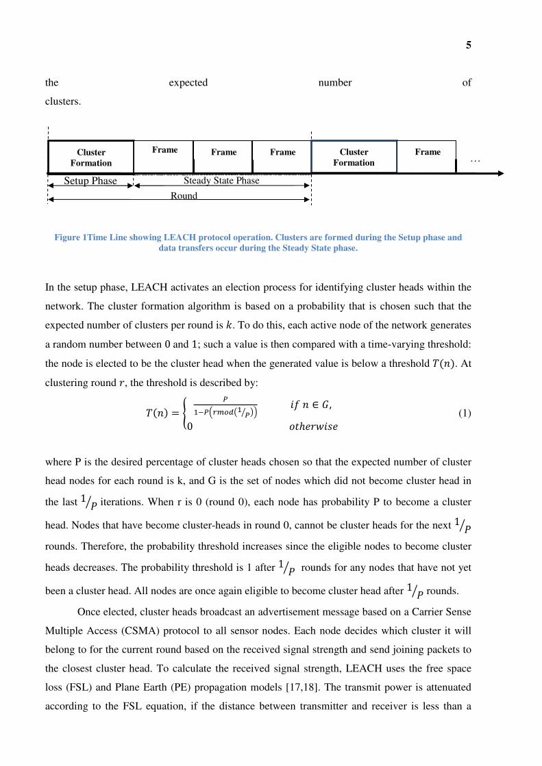
5
the expected number of
clusters.
Figure 1Time Line showing LEACH protocol operation. Clusters are formed during the Setup phase and
data transfers occur during the Steady State phase.
In the setup phase, LEACH activates an election process for identifying cluster heads within the
network. The cluster formation algorithm is based on a probability that is chosen such that the
expected number of clusters per round is �. To do this, each active node of the network generates
a random number between 0 and 1; such a value is then compared with a time-varying threshold:
the node is elected to be the cluster head when the generated value is below a threshold ��. At
clustering round �, the threshold is described by:
�� � ����������� �� �� �� � �,
0 !"#�$�%#& (1)
where P is the desired percentage of cluster heads chosen so that the expected number of cluster
head nodes for each round is k, and G is the set of nodes which did not become cluster head in
the last 1 '� iterations. When r is 0 (round 0), each node has probability P to become a cluster
head. Nodes that have become cluster-heads in round 0, cannot be cluster heads for the next 1 '�
rounds. Therefore, the probability threshold increases since the eligible nodes to become cluster
heads decreases. The probability threshold is 1 after 1 '� rounds for any nodes that have not yet
been a cluster head. All nodes are once again eligible to become cluster head after 1 '� rounds.
Once elected, cluster heads broadcast an advertisement message based on a Carrier Sense
Multiple Access (CSMA) protocol to all sensor nodes. Each node decides which cluster it will
belong to for the current round based on the received signal strength and send joining packets to
the closest cluster head. To calculate the received signal strength, LEACH uses the free space
loss (FSL) and Plane Earth (PE) propagation models [17,18]. The transmit power is attenuated
according to the FSL equation, if the distance between transmitter and receiver is less than a
Frame Cluster
Formation
Frame
…
Setup Phase Steady State Phase
Round
Frame Cluster
Formation
Frame
6
certain cross-over distance. If the distance is greater than a cross-over distance, the transmit
power is attenuated according to the two-ray ground reflection propagation model [14]. The
cross-over point is defined as:
()��**�+,� -.√01231435 (2)
where L is the system loss, "67 and "87 is the transmitting and receiving antenna heights,
respectively, and 9 is the wavelength.
The cluster head receives all join packets and creates a TDMA schedule to specify each
node's time slot to send packets. The cluster creation is performed without taking into
consideration bandwidth limitations. At the end of the setup phase and the network topology
creation, steady state phase begins where nodes are ready to operate: data are acquired from
sensors and forwarded to the cluster head according to the defined TDMA slot schedule.
As illustrated in Figure 1, the steady state operation is divided into several frames for
intra-cluster communication and inter-cluster communication phases. Sensor nodes in each
cluster send data to the cluster head at most once per frame during the allocated time slot. The
duration of each slot is constant, thus the frame duration depends on the number of nodes in the
cluster. If the cluster consists of a larger number of nodes, the frame duration will be longer. The
cluster heads stay awake at all times while the sensor nodes may sleep until its allocated
transmission slot and after transmission over.
In order to reduce energy, each non-cluster head node uses power control to set the
transmit power level. The energy consumed by a transmitter over a short distance (below cross-
over distance) is proportional to the square of the distance between the transceivers, (:, whereas
the energy consumed in a data transmission across longer distances (such as from a cluster head
to the base station) is proportional to (-.
3. Model Validation
To validate the model, various parameters have been studied and simulated results are compared
with the result presented by Heinzelmanet al. [14]. A total of 100 nodes are placed in a grid
topology in an area with dimensions of 100 ; < 100 ; with 10 ; spacing between nodes. The
node placement is based on the tree planting schemes widely used in the plantations where trees
are planted in straight uniformly spaced rows, using a fixed distance between trees within a row
[19]. Based on the tree species, the distance vary and for the purpose of this research, 10m is
selected based on the distance suitable for oil palm and mango plantation [20]. An assumption is
made that each trees in the area needs monitoring, and thus sensor nodes are placed at each tree.
7
The transmitter and receiver antenna height is set to 0.5m ( "= "� 0.5 ;�.Omni-directional
antennas are used at the base station and sensor nodes; that is�= �� 0 (@� with no system
loss A 1�. The wireless channel bit rate is set to 250 kbps at 2.4 �DE radio frequency which
has a wavelength of 0.125 ;. The base station is located in the middle of network topology. All
nodes are initially configured to have a maximum transmission power of 1mW and a receiver
sensitivity value of -85dBm based on Chipcon CC2420 transceiver device specification
[21].Initial battery capacities for all nodes are set to 250 ;F", while base station has unlimited
power supply. Each scenario is evaluated based on the vegetation propagation models to
represents agriculture environments as presented in previous work [17,18]. For each scenario, 10
different seeds are used to simulate the network based on Marsenne twister pseudo-random
number generator.
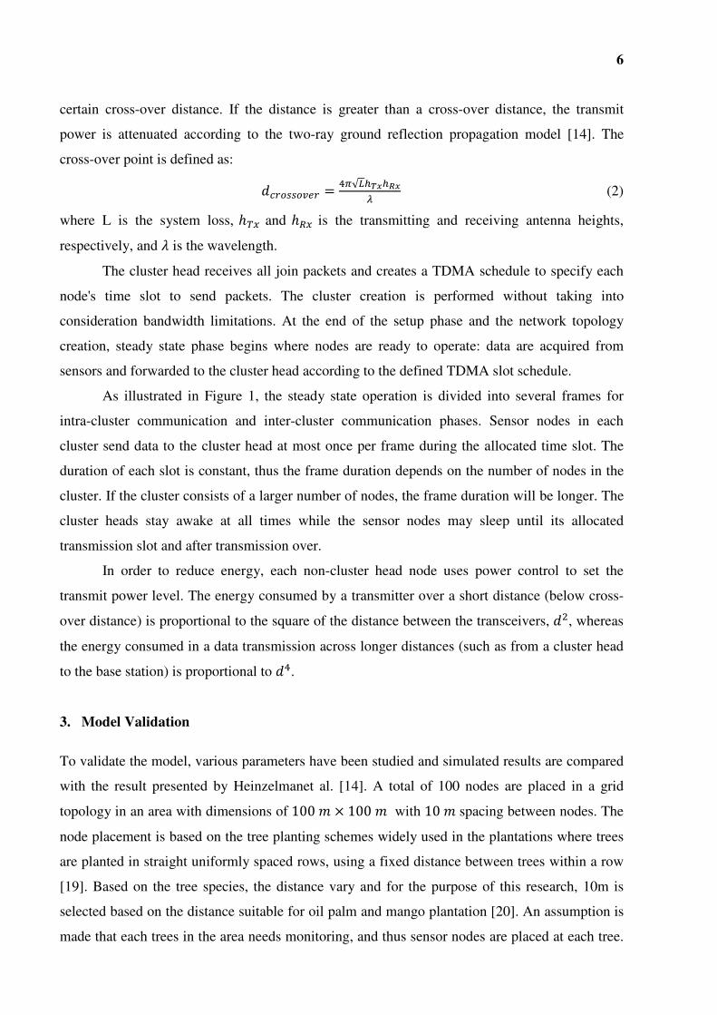
Figure 2, retrieved from Heinzelman et al. [14], shows that the optimal numbers of
clusters in a network of 100 nodes are between 3 and 5. For a verification of LEACH algorithm
that has been implemented in OMNeT++, simulation studies have been performed to evaluate
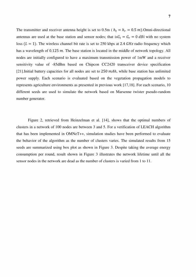
the behavior of the algorithm as the number of clusters varies. The simulated results from 15
seeds are summarized using box plot as shown in Figure 3. Despite taking the average energy
consumption per round, result shown in Figure 3 illustrates the network lifetime until all the
sensor nodes in the network are dead as the number of clusters is varied from 1 to 11.
8
Figure 3 Network Lifetime of LEACH protocol simulated in OMNeT++ until all nodes in the network are
dead as the Number of Cluster varied between 1 and 11
From Figure 3, it is clear that the highest network lifetime is achieved when the number
of clusters is 5 which comply with the results of the original proposed LEACH protocol as
shown in Figure 2. LEACH shows that energy dissipated per round is significantly increased
when the number of clusters is 6 and above. Generated results from OMNeT++, as shown in
Figure 3, illustrates a slower rate of decreasing network lifetime after the number of clusters is 6
when compared to LEACH. This is due to the fact that LEACH implemented in OMNeT++ is
simulated on top of different underlying models such as the radio energy model and radio
Figure 2 Average energy dissipated per round in conventional LEACH protocols retrieved from Heinzelman et al.
[14] as the number of clusters is varied between 1 and 11.
9
propagation model. Nevertheless, it can be observed from the figures that LEACH protocol
implemented in OMNeT++ follows the same behavior as the original LEACH protocol presented
by Heinzelmanet al [14].
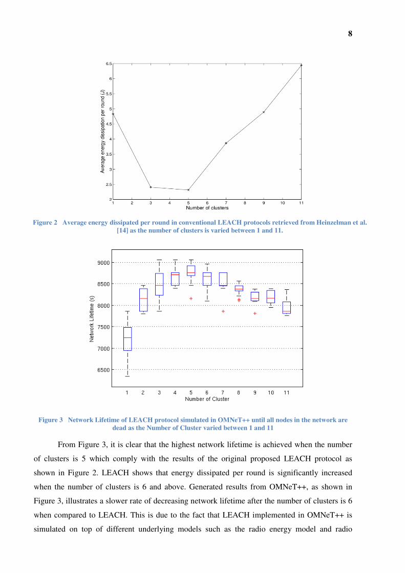
Figure 4 shows the probability threshold, T(n) for the nodes to become cluster head in
each round based on LEACH cluster head selection algorithm simulated in OMNeT++. The
simulated results is based on P=0.05. The probability of each node to become a cluster head is
0.05 when the round is 0. As the number of round increases, the probability increases and
becomes 1 at round 19. At round 19, all sensor nodes that have not yet become cluster head are
selected as the cluster heads. After this round, the probability is once again 0.05.
Figure 4The value of probability threshold, T(n) based on LEACH cluster head selection algorithm when the
percentage of cluster head, P=0.05
4. Protocol Analysis and Discussion
The design of LEACH protocol is, for the most part, efficient and valid and, has been used in
various research works. However, some concerns are raised as to the validity of the evaluation
techniques taken in Heinzelman et al. [14]. This section presents the analysis of LEACH
protocol specifically targeted for agriculture applications.
10
4.1. Radio Propagation Model
The radio propagation model used in LEACH assumes no obstacles in the propagation path and
the received signal power is only affected by the distance between the transmitter and receiver.
All the simulations are based on the FSL and PE propagation models with no consideration of
losses due to the existence of obstacles such as trees in the radio propagation channel. If the
distance between the transmitter and receiver is less than ()��**�+,�, the attenuation is based on
FSL model, and if the distance is greater than ()��**�+,�, the PE model is used. The calculation
for ()��**�+,� is presented in Equation 2.As described in previous studies [17], FSL is suitable
for predicting the signal strength at the receiving node when there is a clear Line of Sight (LOS)
path between the transmitting and receiving nodes [22,23]. The received signal power decreases
with increasing distance between the transceivers. On the other hand, the PE model assumes that
the received signal strength is the sum of the direct LOS propagation path and one ground
reflected component between the source and the destination nodes. However, for obstructed
paths such as in the agriculture application, where there are trees it is not adequate to simply use
FSL and PE propagation models to predict the signal strength. In the previous study reported in
[17,18], it is observed that propagation model used significantly affect the network performance.
When there is vegetation in the radio waves propagation path, the signal undergoes
scattering, absorption and blockage. The congruent effect is additional attenuation of the signal
when compared to losses predicted using FSL or PE models. Based on the studies reported by
Ndzi et al. [18], vegetation attenuation models can be used to model the behavior of radio waves
in agriculture application such as in mango and oil palm plantation. Findings show that in the 2.4
GHz band, FITU-R gives good estimates for low density vegetative environments. For higher
vegetation density environment in a mango plantation, the Non-Zero Gradient (NZG) model
provides consistently low Root Mean Square Error (RMSE) values. Although the NZG model
provides good estimates, it requires more input parameters and is computationally intensive.
Thus, the second best fit model, COST235, can be used to represent this type of environment. In
oil palm plantation, results show that the COST235 model provides consistently low RMSE
values in very high density environments, where there are trees in the line-of-sight path. For
measurements between two rows of palm trees, the path loss can be predicted using FSL model.
The applications of WSNs technology in agriculture includes monitoring various type of
commercially cultivated crops in plantations such as oil palm and rubbers, and also monitoring
high value crops such as medicinal plants and fruits cultivated in artificial conditions. Thus, the
11
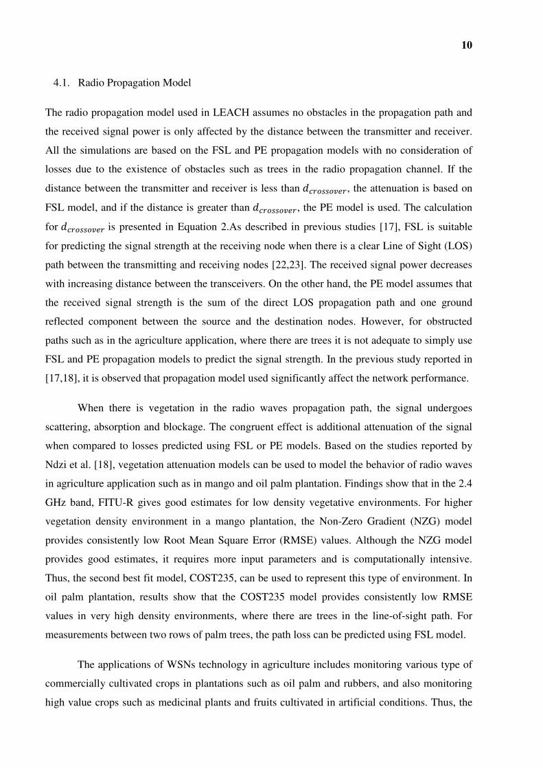
environmental sensors are deployed maybe homogeneously in a mono-crop plantation or
heterogeneously in mixed crops farm area with multiple types of vegetation as shown in Figure
5. A realistic radio propagation model, especially model that can represent the target
environment is important to accurately estimate the performance of algorithms and protocols.
Inaccurate radio propagation models used in simulation to estimate the performance of WSNs
protocols will result in inaccurate performance metrics such as network connectivity, energy
consumptions and network lifetime.
Figure 5 Examples of WSNs node placement in agriculture monitoring
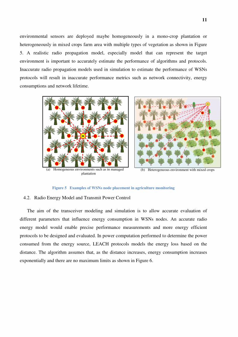
4.2. Radio Energy Model and Transmit Power Control
The aim of the transceiver modeling and simulation is to allow accurate evaluation of
different parameters that influence energy consumption in WSNs nodes. An accurate radio
energy model would enable precise performance measurements and more energy efficient
protocols to be designed and evaluated. In power computation performed to determine the power
consumed from the energy source, LEACH protocols models the energy loss based on the
distance. The algorithm assumes that, as the distance increases, energy consumption increases
exponentially and there are no maximum limits as shown in Figure 6.
(a) Homogeneous environments such as in managed
plantation (b) Heterogeneous environment with mixed crops
12
Figure 6 Energy Consumption during transmission based on LEACH Energy Model
Thus, to transmit an G-bit message at distance d, the energy that the radio expends can be
calculated using equation (3).
H67 IGH,J,) K GLM*(: ( N ()��**�+,�GH,J,) K GL�O(- ( P ()��**�+,� & (3)
where the parameters LM* is based on FSL equations meanwhile, L�O is calculated based on PE
model.To transmit over a short distance (below cross-over distance), the energy consumption is
proportional to the square distance between the transceivers, (:, and based on FSL model. On
the other hand, the energy consumed in a data transmission across longer distances (such as from
a cluster head to the base station) is proportional to (- and calculated based on PE model. Based
on Equation 2, the crossover distance for the experiments described in this research (assuming no
system loss (L=1), transmitting and receiving antenna height of 0.5m and 2.4 GHz radio
frequency) is 21.5m. The power level needed to transmit for a successful reception of data
packets is adjusted based on the distance as given by equation (4).
'67 IQ�'*,R*S=S+S=T(: ( N ()��**�+,�Q:'*,R*S=S+S=T(- ( P ()��**�+,� & (4)
Where Q� -.�UV23V435U, Q: �
V23V43123143 and '*,R*S=S+S=Tis the receiver sensitivity level.
13
It is worth noting that in the conventional LEACH model, energy consumption increases
exponentially with distance and there are no maximum limits. In reality, the transmit power level
of a sensor node can only be adjusted to discrete values that may result in one transmit power
level for multiple distances. Therefore, the resulting energy consumption for two links of
different distances can be equivalent. As discussed in previous study in [24], power consumption
in WSN nodes can be divided into two parts: energy consumed by the on-board electronics
(sensors, display, CPU, etc) and energy consumed by the communication unit. Research has
identified the radio communication unit (in all its modes: transmitting, receiving, idle, listening,
and sleeping) as the main energy consumer [25-27]. The energy required for data transmission is
the orders of magnitude higher than the power spent on data processing. According to Pottie and
Kaiser [25], the amount of energy spent to transmit 1 kb of data to a node located 100 meters
away is equivalent to the energy expended executing 3 million instructions on a general purpose
100 MIPS/W processor. Energy consumption in most devices is non-linear, as part is dissipated
as heat, thermal noise and a fraction is channeled to accomplish the task [27,28]. The former two
energy consumptions are difficult to standardize and they are assumed to be constant.
The total energy, HWXY consumed by �=1 sensor node in Joules is:
HWXY ∑ H*=[=,*=[=, ∑ '*=[=, < !*=[=,�*=[=, (5)
where the index state refers to the operational state of the mote: Sleep, Transmit (Tx),
Receive(Rx) or Idle. Pstate is the power consumed (in Watt) in each state based on the transceiver
specification which can be computed using:
'*=[=, \ < ]*=[=, (6)
The term ]*=[=, denotes the current used by the node in Amperes (A) and V represents the
supply voltage. !*=[=,is the time spent in the corresponding state, which depends on the amount
of information being transmitted or received. This can be calculated using:
!*=[=, 0^_`abc8dYc (7)
whereA�[)e,= is the packet length in bits, and fgS= is the data rate in bps. Table 1 shows
the example of power consumption value and energy consumed by the nodes when transmitting
100 bytes packet based on Chipcon CC2420 radio transceiver [21]. Since the radio
communication unit is the main consumer of the battery power, the energy consumptions of the
14
device’s circuitry (sensors, CPU and display) can reasonably be assumed to be a non-variant
constant.
Table 1Power consumption in each state based on Chipcon CC2420 radio transceiver. Example of energy
consumption, ETxcalculated by setting V=1.8V and L=100 bytes
State Plevel(dBm) Ilevel(mA) PTx(mW) ETx(mJ) Transmit -25 8.53 15.3 0.049
-15 9.64 17.35 0.056 -10 10.68 19.22 0.062 -7 11.86 21.35 0.068 -5 13.11 23.60 0.075 -3 14.09 25.36 0.081 -1 15.07 27.13 0.087 0 16.22 29.20 0.093
Receive - 19.7 35.46 0.113 Sleep - 0.08 0.144 -
4.3. Optimum Number of Cluster
Cluster heads normally spend more energy than cluster member. Therefore, LEACH
proposes to select cluster heads periodically in which each sensor node takes its turn to be a
cluster head. If the probability to become, a cluster head is set high, more nodes will become
cluster heads and the rate of energy consumption also becomes high. However, if the probability
is too low, the size of each cluster becomes large and the average distance between members and
their respective cluster heads increases, which then increases energy consumption. Therefore,
there is a trade-off between the number of clusters and the energy consumption in LEACH.
Figure 2 shows that the optimum number of clusters is between 3 and 5. The network lifetime is
shorter when the number of clusters is below 3. When the number of clusters is less than 3, the
size of each cluster is large, and consequently, the non-cluster head nodes expend more energy to
communicate with the cluster head. LEACH shows that the maximum network lifetime is
achieved when the number of cluster is 5.On the other hand, when the number of clusters is
larger than 6, the number of members in each cluster is small thus, increasing the frequency of
packets transmission from the nodes to the cluster head. As a consequence, the sensor nodes
consume more energy to transmit more data which reduces the sleeping time and the cluster
heads consume more energy to receive more data. Therefore, the network lifetime is reduced
significantly as the number of clusters increases.
4.4. Cluster number variability
The cluster head selection algorithm proposed by LEACH was created to ensure that the
expected number of clusters per round is k. The parameter k was pre-determined to ensure
15
minimum energy dissipation in the network as shown in Figure 2. However, the number of
clusters generated by LEACH in each round varies in a large range around the optimal value,
which shortens the lifetime of the network.
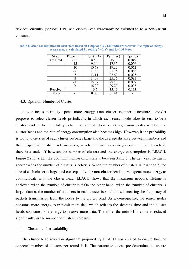
Considering a network of 100 nodes and assuming that the desired number of cluster heads is
5; the desired percentage of cluster head, P, is set to 0.05. Figure 7 shows the distribution of the
number of cluster heads. It can be seen that the number of cluster heads varies in a large range
between 0 and 11. The percentage of rounds that the number of cluster heads is equal to the
target value, 5, is approximately 18% which is less than 25%. In worst cases, there is no cluster
head selected.
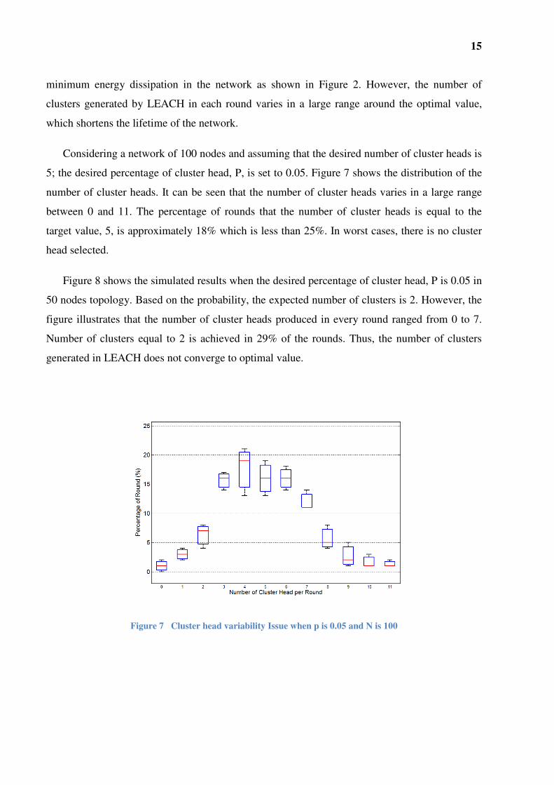
Figure 8 shows the simulated results when the desired percentage of cluster head, P is 0.05 in
50 nodes topology. Based on the probability, the expected number of clusters is 2. However, the
figure illustrates that the number of cluster heads produced in every round ranged from 0 to 7.
Number of clusters equal to 2 is achieved in 29% of the rounds. Thus, the number of clusters
generated in LEACH does not converge to optimal value.
Figure 7 Cluster head variability Issue when p is 0.05 and N is 100
16
Figure 8 Cluster head variability Issue when p is 0.05 and N is 50
4.5. Cluster Distribution
Based on LEACH cluster head selection algorithm, it could be assumed that a selection of
favorable cluster heads in earlier round may result in an unfavorable cluster heads selection
in later rounds since LEACH tries to distribute energy consumption among all nodes. For
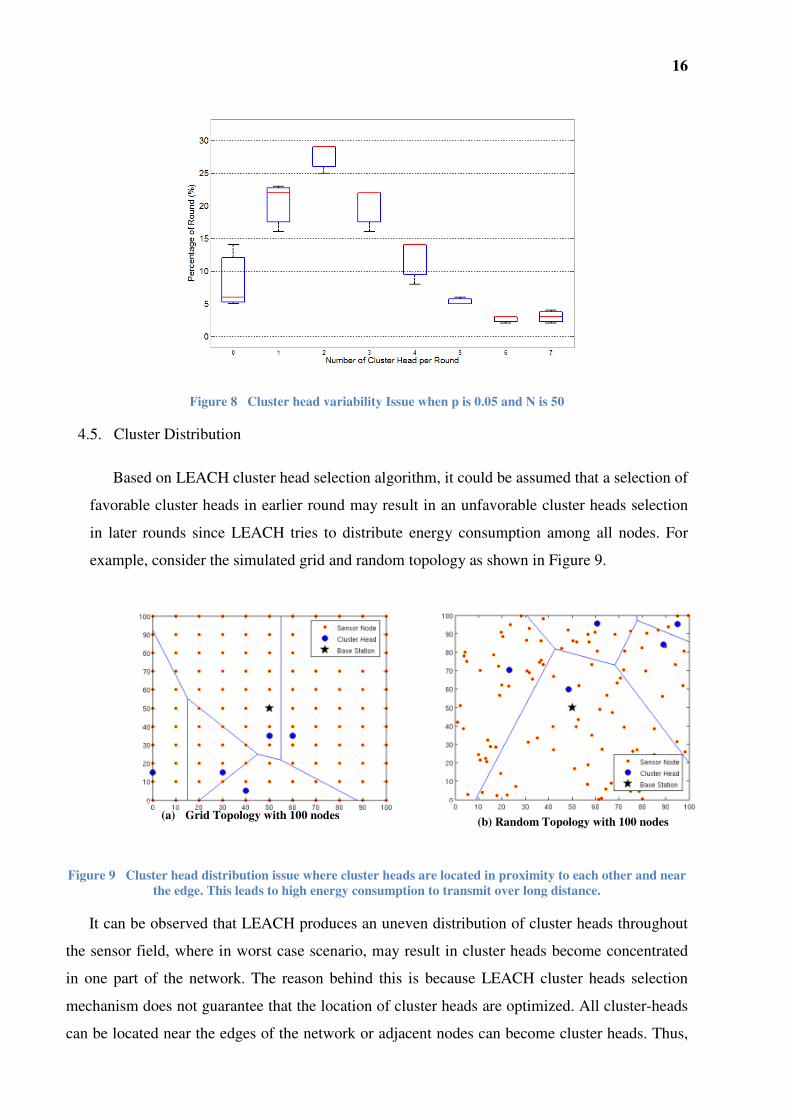
example, consider the simulated grid and random topology as shown in Figure 9.
Figure 9 Cluster head distribution issue where cluster heads are located in proximity to each other and near
the edge. This leads to high energy consumption to transmit over long distance.
It can be observed that LEACH produces an uneven distribution of cluster heads throughout
the sensor field, where in worst case scenario, may result in cluster heads become concentrated
in one part of the network. The reason behind this is because LEACH cluster heads selection
mechanism does not guarantee that the location of cluster heads are optimized. All cluster-heads
can be located near the edges of the network or adjacent nodes can become cluster heads. Thus,
(a) Grid Topology with 100 nodes (b) Random Topology with 100 nodes
17
there could be a number of sensor nodes which are located far from the cluster heads, and as a
result, these nodes will deplete their energy more rapidly as they need higher power to transmit
successfully to their cluster heads. Furthermore, as shown in Figure 9, LEACH protocol does not
also guarantee that nodes are evenly distributed amongst the cluster head nodes [14]. Thus, the
number of member nodes in each cluster is highly variable in LEACH.
4.6. LEACH MAC Layer Protocol
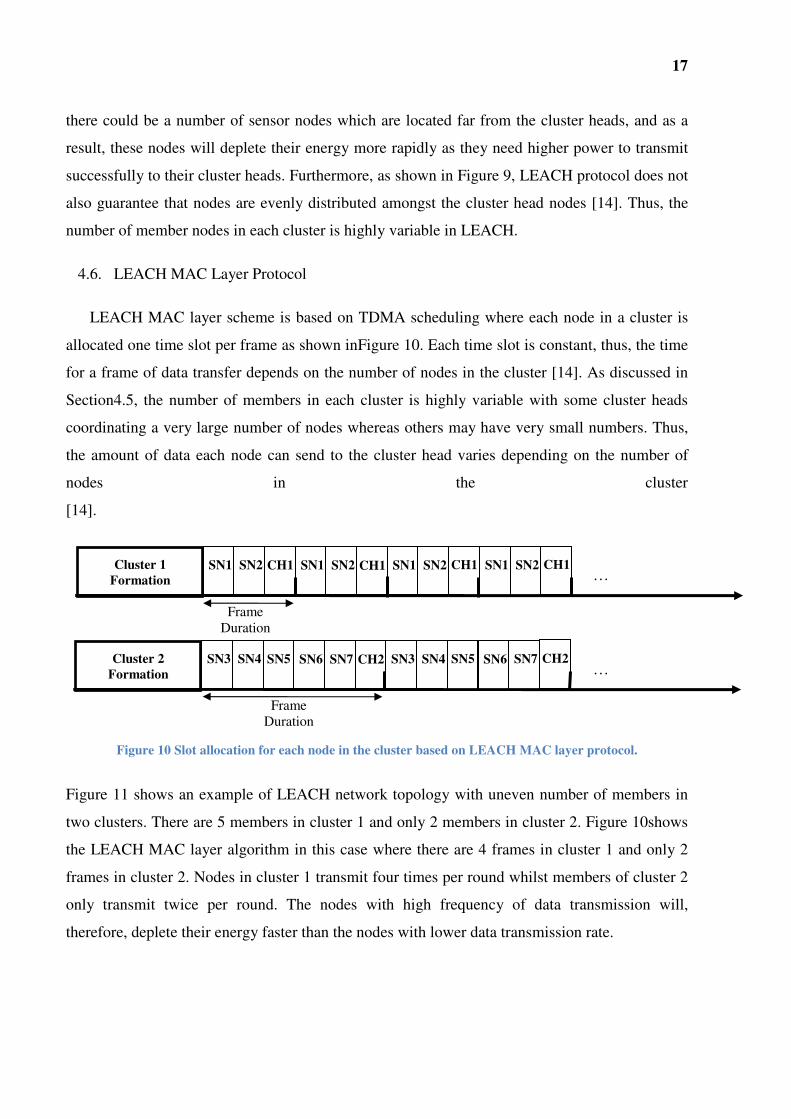
LEACH MAC layer scheme is based on TDMA scheduling where each node in a cluster is
allocated one time slot per frame as shown inFigure 10. Each time slot is constant, thus, the time
for a frame of data transfer depends on the number of nodes in the cluster [14]. As discussed in
Section4.5, the number of members in each cluster is highly variable with some cluster heads
coordinating a very large number of nodes whereas others may have very small numbers. Thus,
the amount of data each node can send to the cluster head varies depending on the number of
nodes in the cluster
[14].
Figure 10 Slot allocation for each node in the cluster based on LEACH MAC layer protocol.
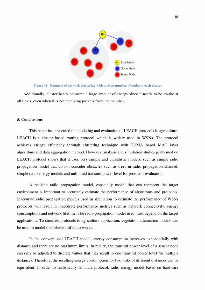
Figure 11 shows an example of LEACH network topology with uneven number of members in
two clusters. There are 5 members in cluster 1 and only 2 members in cluster 2. Figure 10shows
the LEACH MAC layer algorithm in this case where there are 4 frames in cluster 1 and only 2
frames in cluster 2. Nodes in cluster 1 transmit four times per round whilst members of cluster 2
only transmit twice per round. The nodes with high frequency of data transmission will,
therefore, deplete their energy faster than the nodes with lower data transmission rate.
Cluster 2
Formation
Cluster 1
Formation
SN1 SN2 CH1 SN1 SN2 CH1 SN1 SN2 CH1 SN1 SN2 CH1
SN3 SN4 SN5 SN6 SN7 CH2 SN3 SN4 SN5 SN6 SN7 CH2
…
…
Frame
Duration
Frame
Duration
18
Figure 11 Example of network clustering with uneven number of nodes in each cluster
Additionally, cluster heads consume a large amount of energy since it needs to be awake at
all times, even when it is not receiving packets from the member.
5. Conclusions
This paper has presented the modeling and evaluation of LEACH protocols in agriculture.
LEACH is a cluster based routing protocol which is widely used in WSNs. The protocol
achieves energy efficiency through clustering technique with TDMA based MAC layer
algorithms and data aggregation method. However, analysis and simulation studies performed on
LEACH protocol shows that it uses very simple and unrealistic models, such as simple radio
propagation model that do not consider obstacles such as trees in radio propagation channel,
simple radio energy models and unlimited transmit power level for protocols evaluation.
A realistic radio propagation model, especially model that can represent the target
environment is important to accurately estimate the performance of algorithms and protocols.
Inaccurate radio propagation models used in simulation to estimate the performance of WSNs
protocols will result in inaccurate performance metrics such as network connectivity, energy
consumptions and network lifetime. The radio propagation model used must depend on the target
applications. To simulate protocols in agriculture application, vegetation attenuation models can
be used to model the behavior of radio waves.
In the conventional LEACH model, energy consumption increases exponentially with
distance and there are no maximum limits. In reality, the transmit power level of a sensor node
can only be adjusted to discrete values that may result in one transmit power level for multiple
distances. Therefore, the resulting energy consumption for two links of different distances can be
equivalent. In order to realistically simulate protocol, radio energy model based on hardware
19
specifications such as CC2420 can be used to estimate the power consumptions during
transmission, reception, idle listening and sleeping. The radio energy model specifies the
maximum transmit power level and hence limit the sensor node range based on the propagation
environment.
Even though LEACH protocols stated that the optimum number of cluster to prolong
network lifetime is between 3 and 5 in 100 nodes network, the cluster head selection algorithm
shows that the number of cluster heads in each round varies between 0 and 11. In worst case
scenarios, there is no cluster head elected in the round. This indicates that the number of clusters
generated in LEACH does not converge to an optimal value which shortens the lifespan of the
network. Additionally, in agriculture various types of crops exist in the same plantation area.
Each crop needs different types of parameters to be observed and control at different time
intervals. Some of the crops need to be monitored at minute(s) intervals whilst data from other
type of crops are needed only twice a day. This leads to the necessity for a large number of
clusters that are specific to different systems for better farm management.
In some cases, LEACH cluster head selection algorithm produced uneven distribution of
clusters within the network area. All clusterheads can be located near the edges of the network or
adjacent nodes can become cluster heads. In addition, the node scheduling pattern in the LEACH
MAC layer algorithm is not optimized resulting in nodes in different cluster having different data
transmission rates to the cluster head. Therefore, the nodes that have to transmit data to cluster
heads at shorter time intervals deplete their energy faster than the nodes with lower data
transmission rate.
References and Notes
1. Pang, Z., Zheng, L., Tian, J., Kao-Walter, S., Dubrova, E., Chen, Q. Design of a terminal solution for
integration of in-home health care devices and services towards the Internet-of-Things(2015)
Enterprise Information Systems, 9 (1), pp. 86-116.
2. Ramesh, M.V. Design, development, and deployment of a wireless sensor network for detection of
landslides (2014) Ad Hoc Networks, 13 (PART A), pp. 2-18.
3. EmanueleIntrieri, Giovanni Gigli, Francesco Mugnai, Riccardo Fanti, Nicola Casagli, Design and
implementation of a landslide early warning system, Engineering Geology, Volumes 147–148, 12
October 2012, Pages 124-136, ISSN 0013-7952
4. Chiu, J.-C., Dow, C.-R., Lin, C.-M., Lin, J.-H., Hsieh, H.-W.A watershed-based debris flow early
warning system using sensor web enabling techniques in heterogeneous environments(2012) IEEE
Journal of Selected Topics in Applied Earth Observations and Remote Sensing, 5 (6), art. no.
6151221, pp. 1729-1739.
5. Kumar, A., Hancke, G.P. A zigbee-based animal health monitoring system (2015) IEEE Sensors
Journal, 15 (1), art. no. 6945920, pp. 610-617.

20
6. Bitella, G., Rossi, R., Bochicchio, R., Perniola, M., Amato, M. A novel low-cost open-hardware
platform for monitoring soil water content and multiple soil-air-vegetation parameters (2014) Sensors
(Switzerland), 14 (10), pp. 19639-19659.
7. Lloret, J., Garcia, M., Sendra, S., Lloret, G. An underwater wireless group-based sensor network for
marine fish farms sustainability monitoring (2014) Telecommunication Systems, 18 p. Article in
Press
8. Luskin, M.S.; Potts, M.D. Microclimate and habitat heterogeneity through the oil palm lifecycle.
Basic and Applied Ecology,2011, 12, 540-551.
9. Zakaria, A.; Shakaff, A.Y.M.; Masnan, M.J.; Saad, F.S.A.; Adom, A.H.; Ahmad, M.N.; Jaafar, M.N.;
Abdullah, A.H.; Kamarudin, L.M. Improved Maturity and Ripeness Classifications of
MagniferaIndicacv.Harumanis Mangoes through Sensor Fusion of an Electronic Nose and Acoustic
Sensor. Sensors2012, 12, 6023-6048.
10. Zakaria, A.; Shakaff, A.Y.M.; Adorn, A.H.; Ahmad, M.N.; Jaafar, M.N.; Abdullah, A.H.; Fikri, N.A.;
Kamarudin, L.M. Magniferaindica cv. harumanis classification using e-nose. Sensor Letters2011, 9,
359-363.
11. Richard, B.; Dan, T.; Pat, B., Report from the Field: Results from an Agricultural Wireless Sensor
Network. In Proceedings of the 29th Annual IEEE International Conference on Local Computer
Networks, IEEE Computer Society: 2004, Tampa, Florida, U.S.A.
12. Robert, S.; Alan, M.; Joseph, P.; John, A.; David, C., An analysis of a large scale habitat monitoring
application. In Proceedings of the 2nd international conference on Embedded networked sensor
systems, ACM: Baltimore, MD, USA, 2004, 214-226.
13. Kanakaris, V.; Ndzi, D.L.; Ovaliadis, K.; Yang, Y. A new RREQ message forwarding technique
based on Bayesian probability theory, EURASIP Journal on Wireless Communications and
Networking, 2012, 2012:318, 1-12.
14. Heinzelman, W.B.; Chandrakasan, A.P.; Balakrishnan, H. An application-specific protocol
architecture for wireless microsensor networks. Wireless Communications, IEEE Transactions on
2002, 1, 660-670.
15. Huang, B.; Hao, F.; Zhu, H.; Tanabe, Y.; Baba, T. Low-Energy Static Clustering Scheme for
Wireless Sensor Network,International Conference on Wireless Communications, Networking and
Mobile Computing2006, 1-4, Wuhan City, China.
16. Abdul Latiff, N.M.; Tsimenidis, C.C.; Sharif, B.S.; Ladha, C. Dynamic clustering using binary multi-
objective Particle Swarm Optimization for wireless sensor networks.IEEE 19th International
Symposium on Personal, Indoor and Mobile Radio Communications2008, 1-5, Cannes, France.
17. Kamarudin, L.M.; Ahmad, R.B.; Ong, B.L.; Zakaria, A.; Ndzi, D. Modeling and simulation of near-
earth wireless sensor networks for agriculture based application using OMNeT.International
Conference on Computer Applications and Industrial Electronics (ICCAIE)2010, 131-136.
18. Ndzi, D. L.; Kamarudin, L.M.; Muhammad Ezanuddin, A.A; Zakaria, A; Ahmad, R.B; Malek,
M.F.A; Shakaff, A.Y.M; Jafaar, M.N. Vegetation attenuation measurements and modeling in
plantations for wireless sensor network planning, Progress In Electromagnetics Research B2012, 36,
283-301.
19. Wray, P.H. Tree Planting: Planning. Iowa State University Extension 2004, Iowa, U.S.A.
20. Augstburger,F.; Berger, J.; Censkowsky,U.; Heid,P.; Milz, J.; Streit, C. Organic Farming in the
Tropics and Subtropics: Mango. Naturlande.V.2001, 109-118.
21. Chipcon S.R. CC2420 2.4 GHz IEEE 802.15.4 / ZigBee-ready RF Transceiver, 2004,
http://www.ti.com/lit/ds/symlink/cc2420.pdf, accessed 4 July 2015.
22. Seybold, J.S. Introduction to RF Propagation; John Wiley & Sons, 2005, Hoboken, New Jersey.
23. Rappaport, T. Wireless Communications: Principles and Practice(2nd ed.). Prentice Hall PTR, Upper
Saddle River, NJ, USA, 2001.
24. Kamarudin, L.M.; Ahmad, R.B.; Ndzi, D.; Zakaria, A.; Ong, B.L.; Kamarudin, K.; Harun, A.;
Mamduh, S.M. Modeling and Simulation of WSNs for Agriculture Applications Using Dynamic
Transmit Power Control Algorithm.Third International Conference on Intelligent Systems, Modelling
and Simulation (ISMS)2012, 616-621.
25. Pottie, G.J.; Kaiser, W.J. Wireless integrated network sensors. Commun. ACM 2000, 43, 51-58.
26. Förster, A. Teaching Networks How to Learn: Data Dissemination in Wireless Sensor Networks with
Reinforcement Learning; SudwestdeutscherVerlag Fur Hochschulschriften AG: 2009.

21
27. Alan, M.; David, C.; Joseph, P.; Robert, S.; John, A., Wireless sensor networks for habitat
monitoring. In Proceedings of the 1st ACM international workshop on Wireless sensor networks and
applications, ACM: Atlanta, Georgia, USA, 2002, 88-97.
28. Alejandro,M.S.; Jose-Maria,M.G.P; Esteban, E.L; Javier, V.A; Leandro, J.L; Joan, G.H.; An
accurate radio channel model for wireless sensor networks simulation . Communication and Signal
Processing in Sensor Networks2005, 7, 401 - 407.