Seediscussions,stats,andauthorprofilesforthispublicationat:https://www.researchgate.net/publication/260293862

SimulatingCropPhenologicalResponsestoWaterStressUsingthePhenologyMMSSoftwareProgram

ARTICLEinAPPLIEDENGINEERINGINAGRICULTURE·MARCH2013

ImpactFactor:0.41·DOI:10.13031/2013.42654

CITATIONS

3

READS

56

5AUTHORS,INCLUDING:

D.A.Edmunds

UnitedStatesDepartmentofAgriculture

10PUBLICATIONS48CITATIONS

SEEPROFILE

D.C.Nielsen

UnitedStatesDepartmentofAgriculture

119PUBLICATIONS2,158CITATIONS

SEEPROFILE

P.V.VaraPrasad

KansasStateUniversity

149PUBLICATIONS2,909CITATIONS

SEEPROFILE

Allin-textreferencesunderlinedinbluearelinkedtopublicationsonResearchGate,

lettingyouaccessandreadthemimmediately.

Availablefrom:P.V.VaraPrasad

Retrievedon:11February2016

Applied Engineering in Agriculture

Vol. 29(2): 233-249 American Society of Agricultural and Biological Engineers ISSN 0883-8542 233

SIMULATING CROP PHENOLOGICAL RESPONSES TO WATER STRESS USING THE PHENOLOGYMMS

SOFTWARE PROGRAM

G. S. McMaster, J. C. Ascough II, D. A. Edmunds, D. C. Nielsen, P. V. V. Prasad

ABSTRACT. Crop phenology is fundamental for understanding crop growth and development, and increasingly influences many agricultural management practices. Water deficits are one environmental factor that can influence crop phenology through shortening or lengthening the developmental phase, yet the phenological responses to water deficits have rarely been quantified. The objective of this article is to describe the science and general evaluation of a decision support technology software tool, PhenologyMMS (Modular Modeling Software) V1.2. PhenologyMMS was developed to simulate the phenological response of different crops to varying levels of soil water. The program is intended to be simple to use, requires minimal information for calibration, and can be easily incorporated into other crop simulation models. New and revised developmental sequences of the shoot apex correlated with phenological events and the response to soil water availability are provided for proso millet (Panicum milaceum L.), hay/foxtail millet [Setaria italica (L.) P. Beauv.], sunflower (Helianthus annuus L.), and sorghum (Sorghum bicolor L.). Model evaluation consisted of testing algorithms using “generic” default phenology parameters for a crop (i.e., no calibration for specific cultivars was used) for a variety of field experiments to predict developmental events such as seedling emergence, floral initiation, flowering, and physiological maturity. Additionally, an application of the program predicting mean dates of winter wheat (Triticum aestivum L.) phenology across the Central Great Plains based on historical weather records is presented. Results demonstrated that PhenologyMMS has general applicability for predicting crop phenology and offers a simple and easy to use approach to predict and understand how phenology responds to varying water deficits. PhenologyMMS software may be downloaded from http://www.ars.usda.gov/services (select “Software”) or http://arsagsoftware.ars.usda.gov.

Keywords. Crop development, Crop management, Decision support systems, Phenology, Plant growth, Simulation model.

henology, or the sequence and timing of developmental events or stages, is fundamental in understanding crop development and growth. Farmers increasingly are basing management on

crop developmental stages to enhance economic crop yields while maintaining environmental quality. For instance, as non-agricultural demand for water increases, timing limited irrigation water application with critical developmental stages to maximize yield is receiving much interest. Of similar importance, accurate prediction of developmental stages is needed in crop simulation models and decision support tools. Fortunately, a long history of research in plant development and phenology has created significant understanding and ability to predict developmental events.

This is founded on the fundamental concept that plant development is orderly and predictable (Rickman and Klepper, 1995; McMaster, 2005). The genetics of the plant determines the sequence of development (e.g., Distelfeld et al., 2009; Moragues and McMaster, 2011), and environmental conditions (temperature, photoperiod, nutrients, water availability, etc.) can alter the developmental rates (e.g., White et al., 2008).

Most efforts to predict developmental events have focused on the dominant role of temperature, with numerous approaches for quantifying temperature proposed under the general term of thermal time. Several deficiencies remain in accurately predicting phenology in variable environments and management systems. One deficiency is that few studies have examined the impacts of water deficits (degree, timing, and history) on crop phenology (McMaster et al., 2008b), despite the obvious influence of water deficits on some developmental phases (e.g., germination, emergence, grain filling). Furthermore, phenological responses to water deficits vary among crops, cultivars, and developmental events. With few exceptions, crop phenology simulation models do not consider the influence of water deficits on phenology. Compounding the problem of variable phenological responses to water deficits is that for most crops the complete developmental sequence of the shoot apex has not been summarized and quantified or correlated with readily observed

Submitted for review in July 2012 as manuscript number SW 9852;

approved for publication by the Soil & Water Division of ASABE inJanuary 2013.

The authors are Gregory S. McMaster, Research Agronomist,James C. Ascough II, ASABE Member, Research Hydrologic Engineer,Debora A. Edmunds, Research Technician, USDA-Agricultural ResearchService, Agricultural Systems Research Unit, Fort Collins, Colorado USA;David C. Nielsen, Research Agronomist, USDA-ARS-NPA, Central Plains Resource Management Unit, Central Great Plains Research Station,Akron, Colorado USA; and P. V. Vara Prasad, Associate Professor,Department of Agronomy, Kansas State University, Manhattan, KansasUSA. Corresponding author: Gregory S. McMaster, USDA-Agricultural Research Service, Agricultural Systems Research Unit, 2150 Centre Ave.,Bldg. D, Suite 200, Fort Collins, CO 80526 USA; phone: 970-492-7340; e-mail: greg.mcmaster@ars.usda.gov.

P

234 APPLIED ENGINEERING IN AGRICULTURE

developmental stages. These relationships have been developed for a few crops, e.g., wheat, barley, and corn (McMaster et al., 2005), and provide a template to build upon for other crops. Without this fundamental knowledge of development and quantification of phenological responses to water deficits for specific crops, a suitable foundation does not exist for predicting crop development under variable environmental conditions and sharing this knowledge with scientists, producers, and other practitioners.

Such a foundation to transfer knowledge would also aid in developing decision support technologies and parameterization of crop growth sub-models in agroecosystem models such as EPIC (Williams et al., 1989), WEPP (Flanagan et al., 1995), WEPS (Hagen, 1991; Wagner, 1996), SWAT (Arnold et al., 1995), ALMANAC (Kiniry et al., 1992), and GPFARM (McMaster et al., 2002a, 2003a; Ascough et al., 2007). In addition, mechanistic models for certain crops with detailed phenology sub-models such as DSSAT (Jones et al., 2003), APSIM (McCown et al., 1996; Keating et al., 2003), Sirius (Jamieson et al., 1998a, 1998b), and AFRCWHEAT2 (Porter 1984, 1993; Weir et al., 1984) could improve their ability to simulate the effects of environmental factors such as limited soil water. The PhenologyMMS (Modular Modeling Software) V1.2 decision support software tool has recently been developed to simulate the phenology of different crops for varying levels of soil water. McMaster et al. (2011) discussed the interface and provided a general overview of PhenologyMMS; the primary objective of this article is to describe and validate the PhenologyMMS science simulation model. New developmental sequences for sunflower, proso millet, and hay millet that expand on similar developmental sequences previously developed for wheat, barley (Hordeum vulgare L.), corn (Zea mays L.; McMaster et al., 2005) and sorghum (revised from McMaster et al., 2008b) are provided. In addition, general output responses and resultant statistical evaluation of the PhenologyMMS science model are presented, and an application for predicting regional phenology dates for winter wheat is shown.

METHODS AND MATERIALS PHENOLOGYMMS SOFTWARE PROGRAM

To achieve the primary goal of predicting crop phenology, PhenologyMMS software program development focused on three goals: 1) to be as simple as possible to use (i.e., require minimal information or calibration by the user) to facilitate adoption by a variety of users, 2) to incorporate standard programming practices and modularization approaches into the design and programming of the science simulation model (to expedite incorporation into other crop simulation models), and 3) to serve as a learning tool through presentation of detailed crop phenology information to the user. The software program consists of a Java graphical user interface (GUI) integrated with a FORTRAN 95-based simulation model describing crop phenological responses to deficit water

conditions. The GUI has a series of screens to provide default input and parameter databases that can be modified by the user, runs the science simulation model to predict the occurrence of specific developmental stages, and allows users to view the output results. Access to information such as the developmental sequence diagrams of crops, growth staging scales, and supporting documentation is accessed through the interface system and help buttons.

The PhenologyMMS GUI is first used to select the crop and weather file for a site or load a previously created scenario. The following crops are simulated in PhenologyMMS V1.2: winter and spring wheat, winter and spring barley, corn, sorghum, proso millet, hay/foxtail millet, and sunflower. Historical weather data for a variety of sites in the Great Plains are provided (ASCII format), but users may create their own weather files if desired using a pre-defined file template requiring the input of daily maximum/minimum air temperature (in °C) and precipitation (in mm). Required parameter input values (e.g., fig. 1, tables 1-2) are set (based on default values for northeastern Colorado) for each crop upon selection in the PhenologyMMS GUI and discussed in the PhenologyMMS Simulation Model section. However, inputs for certain agronomic practices vary for many reasons and should be changed for the site-specific conditions to be simulated (planting practices are the most likely inputs to modify). The user must select one of four available soil water categories at the time of planting for the depth the seed is planted: optimum, medium, dry, and planted in dust.

Two methods are currently available in PhenologyMMS V1.2 for calculating thermal time as represented by growing degree-days (GDD, °C•day). Once the user has selected a crop, the default method is set based on the most typical approach used for that crop. Regardless of the method for calculating GDD, certain crop-specific (and likely variety-specific) cardinal temperatures are used in the calculations, with default values provided for the base, optimal, and upper/maximum temperatures. Although crops and varieties vary in their rate of leaf appearance (Frank and Bauer, 1995), a default value is provided for each crop and based on the default method for calculating GDD. The final input that can be modified is the maximum potential canopy height of the crop that is used in the canopy height sub-model (discussed in the Phenology Science Simulation model section). Default values for each crop are provided, but the maximum potential canopy height is highly dependent on crop variety. This is particularly true for crops such as wheat and barley with considerable differences between varieties based on the presence or absence of semi-dwarfing genes. However, this input does not influence phenology, so it is not critical if unknown and the user is only interested in simulating phenology.

After selecting a crop, a “generic” cultivar is assumed as the default for each species. Figure 1 illustrates the main inputs needed for the science simulation. If the default generic cultivar is not desired, and depending on the crop, options are provided to select from either a list of varieties or maturity groups using the Variety button at the bottom of the screen. The general layout of this screen is similar for

29(2): 233-249 235

all crops and allows for simulating the progress from one stage to another using either the more common thermal time (“Growing Degree-Days”) or the more developmentally-based (“Number of Leaves”) approaches, both described in the Phenology Science Simulation model section. The other important selection is to choose among the extremes of water stress. The “No Stress” option refers to non-limiting water conditions of soil water availability and should be selected for irrigated or high rainfall conditions. The “Stressed” option refers to conditions of extreme water deficits, but not leading to terminal stress (i.e., just above permanent wilting point). This option

should be selected for most dryland situations where soil water is often severely limiting. Because conditions are often between the “No Stress” and “Stressed” options, either the user can estimate which option is closest to the conditions to be simulated and select that option, or change the default values of one of the options to be intermediate between the two extremes. The default selection for the screen is to use the “No Stress” option and “Growing Degree-Days” method. Any combination of the four options within a row may be selected regardless of selections in the other rows.

Figure 1. Set Growth Stages screen (the default parameters for developmental stages for a generic winter wheat plant are shown). From McMaster et al. (2011).

Table 1. Generic crop default cardinal temperatures and method used to calculate thermal time. Crop

Cardinal Temperatures Winter Wheat

Spring Wheat Corn

Winter Barley

Spring Barley Sunflower Sorghum

Proso Millet

Hay Millet

Base temperature (°C) 0 0 10 0 0 7 10 0 0 Optimal temperature (°C) 18 18 25 18 18 28 25 18 18 Upper threshold temperature °C)[a] NA NA 30 NA NA 30 30 NA NA Method of determining thermal time[b] 1 1 2 1 1 2 2 1 1 [a] NA indicates not used in the thermal time calculation. [b] A description of methods (either 1 or 2) used to calculate thermal time are presented in the Methods section.

Table 2. Germination and seedling elongation rate parameters for specific crops and seedbed conditions. Crop

Soil Moisture Winter Wheat

Spring Wheat

Corn

Winter Barley

Spring Barley

Sunflower

Sorghum

Proso Millet

Hay Millet

Germination (°C•day)[a] Optimum[b] Medium

80.0 90.0

80.0 90.0

30.0 40.0

80.0 90.0

80.0 90.0

40.0 50.0

40.0 50.0

80.0 90.0

80.0 90.0

Dry Dust[c]

110.0 700.0

110.0 700.0

60.0 500.0

110.0 700.0

110.0 700.0

70.0 500.0

70.0 500.0

110.0 700.0

110.0 700.0

Elongation rate (mm °C•day-1) Optimum 0.50 0.50 1.3 0.50 0.50 1.5 1.5 0.50 0.50 Medium 0.40 0.40 1.1 0.40 0.40 1.0 1.0 0.40 0.40 Dry 0.33 0.33 0.7 0.33 0.33 0.6 0.6 0.33 0.33 Dust 0.0 0.0 0.0 0.0 0.0 0.0 0.0 0.0 0.0 Planting depth (cm) 5 4 4.5 4 4 5 5 2 2 [a] Accumulated growing degree-days (GDD) required to initiate germination. [b] Seedbed conditions are based on % water-filled pore space: optimum (>45%), medium (35%-45%), dry (25%-35%), and dust (<25%). [c] Soil moisture in this category is below the minimum threshold to initiate imbibition processes.

236 APPLIED ENGINEERING IN AGRICULTURE

When the simulation model is run, an Output screen is automatically generated. This screen shows the predicted timing of all developmental events (e.g., calendar date, days, and growing degree-days after planting or emergence), the number of leaves produced by the main shoot at the time each developmental event occurred, and final canopy height. Additionally, all information on the initial inputs and parameter values selected is echoed back into the Output screen. The user can save the output screen and also save the simulation scenario (i.e., values selected) if desired, and then retrieve this scenario for further simulation at a later time. A much more extensive description of the PhenologyMMS V1.2 GUI, including all input and output screens, can be found in McMaster et al. (2011).

PHENOLOGYMMS SIMULATION MODEL The primary purpose of the PhenologyMMS V1.2 GUI

is to input the parameters and drivers (e.g., weather) used by the standalone FORTRAN 95 science simulation model. The simulation model is primarily based on:

• Simplifying an earlier and more detailed phenology model for wheat and barley (SHOOTGRO, McMaster et al., 1992b; Zalud et al., 2003), and

• Summarizing and quantifying the entire developmental sequence of the shoot apex of crops and correlating the sequences with commonly used growth stage scales. Particular emphasis was focused on how water deficits impact the phenology of the crop. The template for this synthesis was based on that developed by McMaster et al. (1992a).

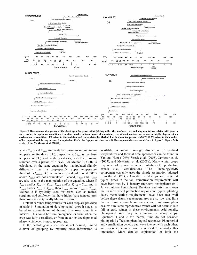
A series of steps were used to create the Set Growth Stages screen (fig. 1) for each crop, which is critical for accurately simulating phenology. An overview describing the steps is provided here. The initial step was to use the entire developmental sequence of the winter wheat shoot apex correlated with developmental stages from commonly used growth stage scales as a template (McMaster, 1997). Once the basic template was developed noting phases such as when leaf primordia are initiated and growing, when new shoots appear, the initiation of inflorescence primordia and internode growth, flowering/anthesis, and physiological maturity, the template could relatively easily be adapted to new crops (particularly grass crops). Developmental sequences for wheat, barley, and corn have been published with supporting documentation (McMaster et al., 2005). The primary difficulties in modifying the template to a new crop were identifying and quantifying when the developmental processes begin and end within the developmental sequence. New developmental sequence diagrams for crops not previously published are presented here for proso millet (fig. 2a), hay millet (fig. 2b), sunflower (fig. 2c), and sorghum (fig. 2d, modified from McMaster et al., 2008b). For proso and hay millet, little developmental information was available; however both crops have developmental sequences very similar to wheat and barley (McMaster et al., 2005) so the wheat template was used. More data were available to create the sunflower developmental sequence, and extensive emphasis was

placed on sources such as Schneiter (1994; 1997), North Dakota State University and Kansas State University Extension information, experts with extensive experience in sunflower production, and unpublished data of the authors. Growth stage scales have been developed for most crops, or are usually easily adapted from another similar crop. For proso millet and hay millet, combinations of the Feekes (Large, 1954), Haun (1973), Waldron and Flowerday (1979), and Zadoks et al. (1974) growth stage scales were used, and sunflower was based on Schneiter and Miller (1981) and Schneiter et al. (1998). The sorghum developmental sequence diagram originally published in McMaster et al. (2008b) estimated the time of jointing too late and this was revised as shown in figure 2d. We also added the developmental stage for the beginning of tiller initiation (TI).

Once the developmental sequence diagrams under optimal conditions were created for a generic crop (e.g., figs. 2a-d), the relationship between developmental stages considered by growth stage scales and additional developmental stages occurring at the shoot apex were established. It was then necessary to determine the sequential phenological responses of all developmental events to water deficits. Templates for these diagrams for proso millet, hay millet, sunflower, and sorghum (figs. 3a-d) were based on those previously developed for wheat, barley, and corn (McMaster et al., 2005). General phenological data for proso and hay millet were not readily available, and particularly were limited for phenological responses to water deficits. Therefore, relationships were quantified largely based on wheat. More data were available for sunflower and a number of sources (e.g., Goyne et al., 1977; Yegappan et al., 1980; Marc and Palmer, 1981; Unger, 1983; Connor and Jones, 1985; Schneiter, 1997; Aiken, 2005; others listed above, and citations within these sources) provided some of the required information. The overall sequence was then reviewed by experts in sunflower development and compared to general expectations when particular key developmental stages were expected within a region as a general test. The phenological responses to water deficits diagrams (figs. 3a-d) were then used to develop the Set Growth Stages screen (fig. 1) in the PhenologyMMS program, and new crops can be readily added based on these diagrams.

The Set Growth Stages screen (fig. 1) uses the thermal time method selected by the user. Currently two methods for calculating thermal time are allowed in PhenologyMMS and further described in McMaster and Wilhelm (1997). Although both methods are very similar, with few differences in accuracy between them for programs such as PhenologyMMS, differences up to 30% in accumulated thermal time as calculated in growing degree-days (GDD,

°C•day) can occur between the two methods. The GDD calculated according to Method 1 is:

1

02

nmax,i min,i

basei

T TGDD T GDD

=

+ = − ≥

(1)

29(2): 233-249 237

where Tmax,i and Tmin,i are the daily maximum and minimum temperature for day i (°C), respectively, Tbase is the base temperature (°C), and the daily values greater than zero are summed over a period of n days. For Method 2, GDD is calculated by the same equation but manipulated slightly differently. First, a crop-specific upper temperature threshold (Tupper, °C) is included, and additional GDD above Tupper are not accumulated. Second, Tbase and Tupper are also used in the manipulation of the equation, where if Tmax,i and/or Tmin,i < Tbase, Tmax,i and/or Tmin,i = Tbase and if Tmax,i and/or Tmin,i > Tupper, then Tmax,i and/or Tmin,i = Tupper. Method 2 is typically used for crops such as maize, sorghum, and sunflower that have higher base temperatures than crops where typically Method 1 is used.

Default cardinal temperatures for each crop are provided in table 1. Simulation of developmental growth stages is based on accumulation of thermal time over some time interval. This could be from emergence, or from when the crop was fully vernalized, or from an earlier developmental phase, whichever is most appropriate.

If the default generic cultivar is not desired, limited cultivar or grouping by maturity class information is

available. A more thorough discussion of cardinal temperatures and thermal time approaches can be found in Yan and Hunt (1999), Streck et al. (2003), Jamieson et al. (2007), and McMaster et al. (2008a). Many winter crops require a cold period to induce initiation of reproductive events (i.e., vernalization). The PhenologyMMS component currently uses the simple assumption adopted from the SHOOTGRO model that if crops are planted at typical times in the fall, vernalization requirements will have been met by 1 January (northern hemisphere) or 1 July (southern hemisphere). Previous analysis has shown that in most wheat production regions and typical planting dates, vernalization requirements have been met well before these dates, yet temperatures are so low that little thermal time accumulation occurs and this assumption ensures simulated reproductive events will not occur in late fall or early winter in these environments. Additionally, photoperiod sensitivity is common in many crops. Equations 1 and 2 for thermal time do not consider photoperiod effects on phenological responses. Photoperiod and vernalization genetic pathways interact with each other, and various methods have been used to consider this interaction. More detailed explanation of both the

Figure 2. Developmental sequence of the shoot apex for proso millet (a), hay millet (b), sunflower (c), and sorghum (d) correlated with growth stage scales for optimum conditions. Question marks indicate areas of uncertainty, significant cultivar variation, or highly dependent on environmental conditions. TT refers to thermal time and is calculated by Method 1 with a base temperature of 0°C. #LVS refers to the number of leaves produced during interval (or equivalent if after leaf appearance has ceased). Developmental events are defined in figure 3. Figure 2d is revised from McMaster et al. (2008b).

(a) (b)

(c) (d)

238 APPLIED ENGINEERING IN AGRICULTURE

vernalization and photoperiod equations are available in Jamieson et al. (2007) and McMaster et al. (2008a).

Although most crop simulation models use some form of a thermal time approach, a more developmentally-based approach using the phyllochron (defined as the thermal time required between the appearance of successive leaves on a shoot) has gained acceptance among developmental physiologists. In this approach, rather than use a static thermal time estimate between developmental events, the number of leaves formed between the developmental events is used. Although very similar to the thermal time approach, the phyllochron approach is more dynamic as it can change both during the ontogeny of the plant and among planting dates and seems to be a better integrator of shoot developmental events (Rickman and Klepper, 1995). Unfortunately, information and knowledge on the phyllochron isn’t always readily available for many crops/cultivars. The PhenologyMMS component uses a constant phyllochron throughout the life cycle provided as a default parameter (determined by literature searches). If the number of leaves required between two developmental events is not known, then the thermal time equivalent is used and divided by the phyllochron to obtain the number of leaves. Although equations to predict the phyllochron

have been proposed for certain crops such as wheat, accuracy of predictions are often poor (e.g., McMaster and Wilhelm, 1995).

If the PhenologyMMS simulation model is incorporated into a plant growth model with a soil water balance component, then the user does not need to select between the “No Stress”, intermediate, or “Stressed” conditions previously described. Rather, a simulated water stress factor can be used to adjust between the extreme values. Simple linear regressions are used to interpolate between the default “No Stress” and “Stressed” values (fig. 4). Threshold values for a water stress factor are set at 0.8, where it is assumed that plant water deficits above this are not limiting, and at 0.4, below which no further adjustment to water deficits is expected. Determining the 0-1 water stress factor can be done many ways, but some common methods are to predict the ratios of actual evapotranspiration/potential evapotranspiration or available soil water/potential available soil water.

OTHER PHENOLOGYMMS SIMULATION COMPONENTS Two other science modules are included in

PhenologyMMS: seedling emergence and canopy height. The seedling emergence model is a simplified version of

Figure 3. Proso millet (a), hay millet (b), sunflower (c), and sorghum (d) phenological responses to water availability. TT refers to “thermal time” and #LVS refers to the “number of leaves” produced during interval (or equivalent if after leaf appearance has ceased). Figure 3d is revised from McMaster et al. (2008b).

(a)

(c) (d)

(b)

29(2): 233-249 239

that incorporated into the SHOOTGRO model (Wilhelm et al., 1993). The period from sowing to emergence consists of two distinct sub-phases: the start of imbibition leading to germination and protrusion of the radicle from the seed resulting in appearance of the cotyledons above the soil surface (Bewley and Black, 1985). As Connor and Hall (1997) note, agronomic experiments rarely distinguish among these sub-phases making interpretation of experimental results difficult. Yet differentiating among the two sub-phases is important in developing a module that is robust across variable environments. PhenologyMMS considers three factors to control the date of seedling emergence: soil moisture near the seed, temperature, and planting depth. For most crops, soil moisture primarily controls the first sub-phase of the beginning of imbibition and thermal time to germination (Germ, °C•day):

( )GDDreq

ii planting day

Germ GDD=

= (2)

where the daily growing degree-days (GDDi, °C•day) is summed from planting day until the required number of growing degree-days for germination to occur, based on the soil moisture conditions of the seedbed zone, is reached (GDDreq, °C•day). Table 2 presents the default crop-specific values for GDDreq, and GDD are currently calculated using either Method 1 (eq. 1) or 2 selected for the crop. Precisely determining these parameters is difficult

for various reasons. In addition to limited data measuring germination under field conditions, general classifications of soil moisture in the top soil layer usually do not reflect the micro-environment of the seed within the soil layer. Numerous seed germination experiments have shown that under conditions with excellent contact of the seed with water and high humidity as found in petri dishes, imbibition for some crops can occur and the radicle begin to appear within a day (e.g., Hernandez and Orioli, 1985 for sunflower; Wilhelm et al., 1993 for wheat; and unpublished data of McMaster for wheat). Yet the authors have never observed this in the field, and generally under “optimal” water conditions it takes at least a couple days for germination to occur. Other crops can have longer periods required for imbibition to occur depending on many factors, particularly whether dormancy is present which is not considered in this module. Based on this general knowledge and observations, parameters for the thermal time required for germination under optimal conditions (GDDreq) were often set to be at least half of the thermal time required from sowing to emergence expected for a crop.

Once germination has occurred, temperature primarily drives the daily elongation (Elongationi, cm) of the shoot from the seed:

( /10)i i iElongation ElongRate GDD= ∗ (3)

where ElongRatei is the shoot elongation rate (mm °C•day-1) for day i based on the soil water content (see table 2 for default crop-specific values) and GDDi is as previously defined. Seedling emergence occurs when the cumulative elongation is ≥ planting depth. When data could be found, the shoot growth elongation rate parameters were derived from germination studies giving the rate of radicle elongation for given temperatures.

Crop-specific parameters for germination and elongation rate in table 2 are based on four general categories of soil moisture in the seedbed layer: optimum (> 45% water-filled pore space), medium (35%-45%), dry (25%-35%), and planted in dust (< 25%). These values do not need to be precisely estimated; rather the user can choose the category based on general conditions. The stand-alone version of PhenologyMMS does not have a soil water balance module, so a surrogate approach to vary soil moisture conditions while simulating seedling emergence is to use precipitation during this time period. Daily rainfall amounts from 5- to 7-mm increments the soil moisture category to the next higher level of soil moisture. If rainfall events are from 7 to 12 mm, the soil moisture category is incremented two levels. If the starting level of soil moisture is planted in dust, then accumulation of thermal time does not begin until the soil moisture category is at least dry.

The canopy height module allows for two phases of canopy growth. Depending on the crop, these two phases may not be completely distinct, but for crops such as winter wheat and winter barley the first phase applies to the prostrate growth habit from emergence in the fall until the beginning of internode elongation in the spring. The second phase is the period of greatest increase in plant height

Figure 4. Adjusting thermal time or number of leaves required toreach a developmental event as a function of water stress. Inputvalues for the thermal time (as growing degree-days, GDD) or leafnumber required for the extreme conditions of non-limiting water deficits “No stress”) or water-limiting deficits (i.e., just abovepermanent wilting point; “Stress”) are adjusted for intermediatevalues of water stress. Water stress is represented by a 0-1 water stress factor that can be calculated many ways. Figure 4a shows thecase where water stress results in the developmental event occurringearlier (i.e., fewer GDD required); figure 4b shows the opposite casewhere water stress delays the developmental event.

240 APPLIED ENGINEERING IN AGRICULTURE

resulting from internode elongation pushing the shoot apex (i.e., the developing spike) through the whorl of leaves and above the leaf canopy. For simplicity, a linear daily growth rate in canopy height (CanopyHti, cm) is assumed during each phase as:

1i i i iCanopyHt CanopyHt ( HtRate GDDday )−= + ∗ (4)

where CanopyHti for day i is determined by the daily increase in canopy height (HtRatei, cm °C•day-1) and the growing degree-days for the day (GDDdayi, °C•day). HtRatei is calculated for day i during each phase as:

j

ij

FinalMaxHtHtRate

GDDsum= (5)

where the final maximum potential height (FinalMaxHtj , cm) of each phase (j = 1 or 2) is an input parameter and GDDsumj (°C•day) is the sum of the growing degree-days for phase 1 or 2 (based on figs. 1 and 3). Phase 2 for most crops (e.g., wheat, barley, corn, sorghum, millet) should normally begin at the start of internode elongation (just before the stage of jointing when the first node appears above the soil surface) and end near the time of flowering/anthesis. However, for ease of obtaining data and simplicity, the model is set to begin Phase 2 at the stage of jointing and end at the beginning of flowering/anthesis. Currently the growth rate is not reduced by water deficits, so the maximum potential canopy height is simulated. The maximum potential canopy height at the end of Phase 2 is very genotype dependent, and parameter values often are readily available from seed companies.

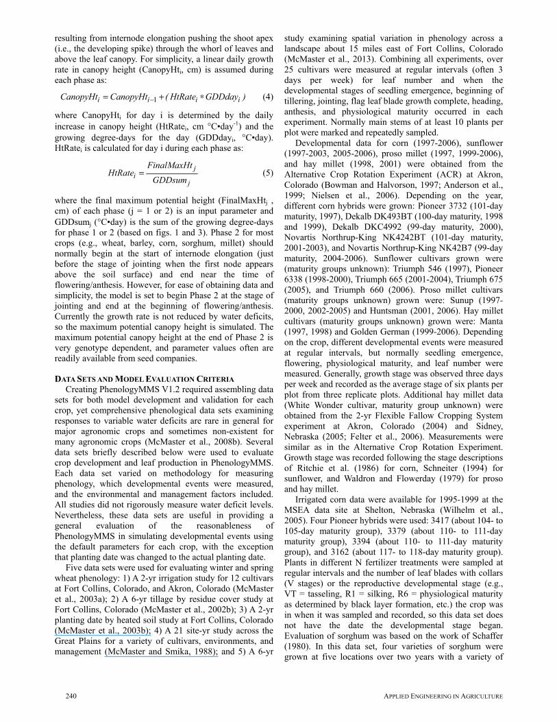
DATA SETS AND MODEL EVALUATION CRITERIA Creating PhenologyMMS V1.2 required assembling data

sets for both model development and validation for each crop, yet comprehensive phenological data sets examining responses to variable water deficits are rare in general for major agronomic crops and sometimes non-existent for many agronomic crops (McMaster et al., 2008b). Several data sets briefly described below were used to evaluate crop development and leaf production in PhenologyMMS. Each data set varied on methodology for measuring phenology, which developmental events were measured, and the environmental and management factors included. All studies did not rigorously measure water deficit levels. Nevertheless, these data sets are useful in providing a general evaluation of the reasonableness of PhenologyMMS in simulating developmental events using the default parameters for each crop, with the exception that planting date was changed to the actual planting date.

Five data sets were used for evaluating winter and spring wheat phenology: 1) A 2-yr irrigation study for 12 cultivars at Fort Collins, Colorado, and Akron, Colorado (McMaster et al., 2003a); 2) A 6-yr tillage by residue cover study at Fort Collins, Colorado (McMaster et al., 2002b); 3) A 2-yr planting date by heated soil study at Fort Collins, Colorado (McMaster et al., 2003b); 4) A 21 site-yr study across the Great Plains for a variety of cultivars, environments, and management (McMaster and Smika, 1988); and 5) A 6-yr

study examining spatial variation in phenology across a landscape about 15 miles east of Fort Collins, Colorado (McMaster et al., 2013). Combining all experiments, over 25 cultivars were measured at regular intervals (often 3 days per week) for leaf number and when the developmental stages of seedling emergence, beginning of tillering, jointing, flag leaf blade growth complete, heading, anthesis, and physiological maturity occurred in each experiment. Normally main stems of at least 10 plants per plot were marked and repeatedly sampled.

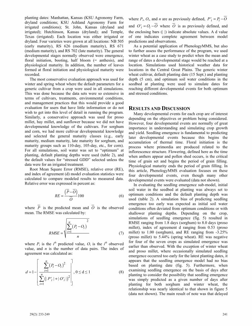
Developmental data for corn (1997-2006), sunflower (1997-2003, 2005-2006), proso millet (1997, 1999-2006), and hay millet (1998, 2001) were obtained from the Alternative Crop Rotation Experiment (ACR) at Akron, Colorado (Bowman and Halvorson, 1997; Anderson et al., 1999; Nielsen et al., 2006). Depending on the year, different corn hybrids were grown: Pioneer 3732 (101-day maturity, 1997), Dekalb DK493BT (100-day maturity, 1998 and 1999), Dekalb DKC4992 (99-day maturity, 2000), Novartis Northrup-King NK4242BT (101-day maturity, 2001-2003), and Novartis Northrup-King NK42B7 (99-day maturity, 2004-2006). Sunflower cultivars grown were (maturity groups unknown): Triumph 546 (1997), Pioneer 6338 (1998-2000), Triumph 665 (2001-2004), Triumph 675 (2005), and Triumph 660 (2006). Proso millet cultivars (maturity groups unknown) grown were: Sunup (1997-2000, 2002-2005) and Huntsman (2001, 2006). Hay millet cultivars (maturity groups unknown) grown were: Manta (1997, 1998) and Golden German (1999-2006). Depending on the crop, different developmental events were measured at regular intervals, but normally seedling emergence, flowering, physiological maturity, and leaf number were measured. Generally, growth stage was observed three days per week and recorded as the average stage of six plants per plot from three replicate plots. Additional hay millet data (White Wonder cultivar, maturity group unknown) were obtained from the 2-yr Flexible Fallow Cropping System experiment at Akron, Colorado (2004) and Sidney, Nebraska (2005; Felter et al., 2006). Measurements were similar as in the Alternative Crop Rotation Experiment. Growth stage was recorded following the stage descriptions of Ritchie et al. (1986) for corn, Schneiter (1994) for sunflower, and Waldron and Flowerday (1979) for proso and hay millet.

Irrigated corn data were available for 1995-1999 at the MSEA data site at Shelton, Nebraska (Wilhelm et al., 2005). Four Pioneer hybrids were used: 3417 (about 104- to 105-day maturity group), 3379 (about 110- to 111-day maturity group), 3394 (about 110- to 111-day maturity group), and 3162 (about 117- to 118-day maturity group). Plants in different N fertilizer treatments were sampled at regular intervals and the number of leaf blades with collars (V stages) or the reproductive developmental stage (e.g., VT = tasseling, R1 = silking, R6 = physiological maturity as determined by black layer formation, etc.) the crop was in when it was sampled and recorded, so this data set does not have the date the developmental stage began. Evaluation of sorghum was based on the work of Schaffer (1980). In this data set, four varieties of sorghum were grown at five locations over two years with a variety of

29(2): 233-249 241

planting dates: Manhattan, Kansas (KSU Agronomy Farm, dryland conditions; KSU Ashland Agronomy Farm for irrigated conditions); St. John, Kansas (dryland and irrigated); Hutchinson, Kansas (dryland); and Temple, Texas (irrigated). Each location was either irrigated or dryland. Four varieties were grown at all locations: NB 505 (early maturity), RS 626 (medium maturity), RS 671 (medium maturity), and RS 702 (late maturity). The general developmental stages normally observed were emergence, floral initiation, booting, half bloom (= anthesis), and physiological maturity. In addition, the number of leaves formed at floral initiation and physiological maturity were recorded.

The most conservative evaluation approach was used for winter and spring wheat where the default parameters for a generic cultivar from a crop were used in all simulations. This was done because the data sets were so extensive in terms of cultivars, treatments, environmental conditions, and management practices that this would provide a good evaluation for users that have little information or do not wish to get into this level of detail in running the program. Similarly, a conservative approach was used for proso millet, hay millet, and sunflower because we did not have developmental knowledge of the cultivars. For sorghum and corn, we had more cultivar developmental knowledge and selected the general maturity classes (e.g., early maturity, medium maturity, late maturity for sorghum, and maturity groups such as 110-day, 105-day, etc., for corn). For all simulations, soil water was set to “optimum” at planting, default planting depths were used (table 2), and the default values for “stressed GDD” selected unless the data were for an irrigated treatment.

Root Mean Square Error (RMSE), relative error (RE), and index of agreement (d) model evaluation statistics were calculated to compare modeled results to measured data. Relative error was expressed in percent as:

( )

100P O

REO

−= (6)

where P is the predicted mean and O is the observed mean. The RMSE was calculated by:

( )2

1

n

i ii

P O

RMSEn

=−

=

(7)

where Pi is the ith predicted value, Oi is the ith observed value, and n is the number of data pairs. The index of agreement was calculated as:

( )

( )

2

1

2

1

1

n

i ii

n

i ii

P O

d

| P' | | O' |

=

=

−

= − +

, 0 ≤ d ≤ 1 (8)

where Pi, Oi, and n are as previously defined, i iP' P O= −

and i iO' O O= − where O is as previously defined, and

the enclosing bars (| |) indicate absolute values. A d value of one indicates complete agreement between model predictions and observations.

As a potential application of PhenologyMMS, but also to further assess the performance of the program, we used winter wheat as a case study to predict when the mean and range of dates a developmental stage would be reached at a location. Simulations used historical weather data for locations in the Central Great Plains. The generic winter wheat cultivar, default planting date (15 Sept.) and planting depth (5 cm), and optimum soil water conditions in the seedbed at planting were used to simulate dates for reaching different developmental events for both optimum and stressed conditions.

RESULTS AND DISCUSSION Many developmental events for each crop are of interest

depending on the objectives or problem being considered. However, four developmental events are normally of great importance in understanding and simulating crop growth and yield. Seedling emergence is fundamental to predicting later developmental events because this begins the accumulation of thermal time. Floral initiation is the process where primordia are produced related to the inflorescence structure. Flowering, defined here as the time when anthers appear and pollen shed occurs, is the critical time of grain set and begins the period of grain filling. Physiological maturity ends the period of grain filling. In this article, PhenologyMMS evaluation focuses on these four developmental events, even though many other developmental events were evaluated (data not shown).

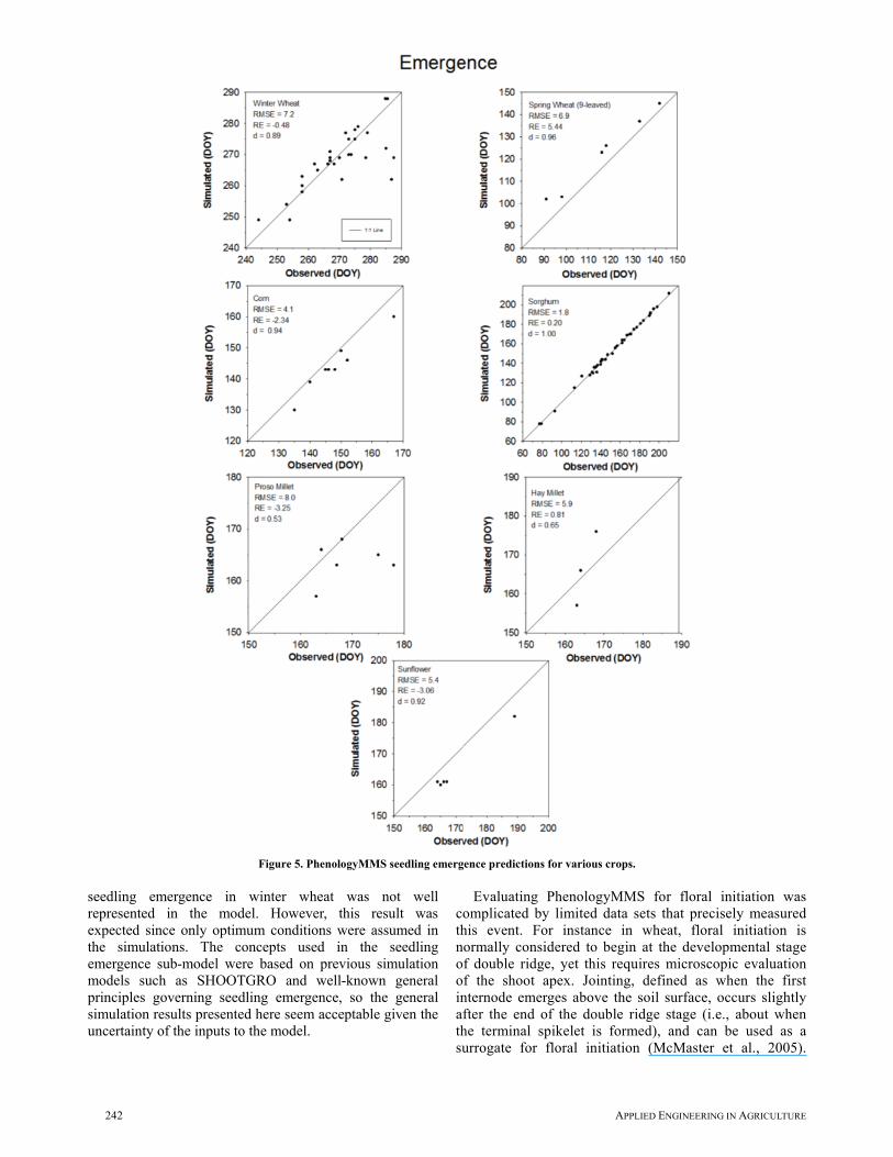
In evaluating the seedling emergence sub-model, initial soil water in the seedbed at planting was always set to optimum conditions and the default planting depth was used (table 2). A simulation bias of predicting seedling emergence too early was expected as initial soil water conditions often deviated from optimum conditions or with shallower planting depths. Depending on the crop, simulations of seedling emergence (fig. 5) resulted in RMSE ranging from 1.8 days (sorghum) to 8.0 days (proso millet), index of agreement d ranging from 0.53 (proso millet) to 1.00 (sorghum), and RE ranging from -3.25% (proso millet) to 5.44% (spring wheat). RE was negative for four of the seven crops as simulated emergence was earlier than observed. With the exception of winter wheat and proso millet, where occasionally simulated seedling emergence occurred too early for the latest planting dates, it appears that the seedling emergence model had no bias based on planting date (fig. 5). Furthermore, when examining seedling emergence on the basis of days after planting to consider the possibility that seedling emergence was simply predicted as a given number of days after planting for both sorghum and winter wheat, the relationship was nearly identical to that shown in figure 5 (data not shown). The main result of note was that delayed

242 APPLIED ENGINEERING IN AGRICULTURE

seedling emergence in winter wheat was not well represented in the model. However, this result was expected since only optimum conditions were assumed in the simulations. The concepts used in the seedling emergence sub-model were based on previous simulation models such as SHOOTGRO and well-known general principles governing seedling emergence, so the general simulation results presented here seem acceptable given the uncertainty of the inputs to the model.

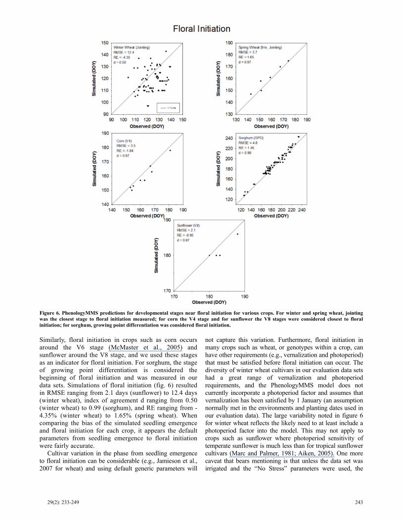
Evaluating PhenologyMMS for floral initiation was complicated by limited data sets that precisely measured this event. For instance in wheat, floral initiation is normally considered to begin at the developmental stage of double ridge, yet this requires microscopic evaluation of the shoot apex. Jointing, defined as when the first internode emerges above the soil surface, occurs slightly after the end of the double ridge stage (i.e., about when the terminal spikelet is formed), and can be used as a surrogate for floral initiation (McMaster et al., 2005).

Figure 5. PhenologyMMS seedling emergence predictions for various crops.

29(2): 233-249 243

Similarly, floral initiation in crops such as corn occurs around the V6 stage (McMaster et al., 2005) and sunflower around the V8 stage, and we used these stages as an indicator for floral initiation. For sorghum, the stage of growing point differentiation is considered the beginning of floral initiation and was measured in our data sets. Simulations of floral initiation (fig. 6) resulted in RMSE ranging from 2.1 days (sunflower) to 12.4 days (winter wheat), index of agreement d ranging from 0.50 (winter wheat) to 0.99 (sorghum), and RE ranging from -4.35% (winter wheat) to 1.65% (spring wheat). When comparing the bias of the simulated seedling emergence and floral initiation for each crop, it appears the default parameters from seedling emergence to floral initiation were fairly accurate.

Cultivar variation in the phase from seedling emergence to floral initiation can be considerable (e.g., Jamieson et al., 2007 for wheat) and using default generic parameters will

not capture this variation. Furthermore, floral initiation in many crops such as wheat, or genotypes within a crop, can have other requirements (e.g., vernalization and photoperiod) that must be satisfied before floral initiation can occur. The diversity of winter wheat cultivars in our evaluation data sets had a great range of vernalization and photoperiod requirements, and the PhenologyMMS model does not currently incorporate a photoperiod factor and assumes that vernalization has been satisfied by 1 January (an assumption normally met in the environments and planting dates used in our evaluation data). The large variability noted in figure 6 for winter wheat reflects the likely need to at least include a photoperiod factor into the model. This may not apply to crops such as sunflower where photoperiod sensitivity of temperate sunflower is much less than for tropical sunflower cultivars (Marc and Palmer, 1981; Aiken, 2005). One more caveat that bears mentioning is that unless the data set was irrigated and the “No Stress” parameters were used, the

Figure 6. PhenologyMMS predictions for developmental stages near floral initiation for various crops. For winter and spring wheat, jointing was the closest stage to floral initiation measured; for corn the V4 stage and for sunflower the V8 stages were considered closest to floralinitiation; for sorghum, growing point differentiation was considered floral initiation.

244 APPLIED ENGINEERING IN AGRICULTURE

“Stressed” parameters used represented the extreme phenological responses to water deficits and would also lead to a slightly earlier or later prediction of floral initiation depending on whether water deficits hasten or delay floral initiation of the crop.

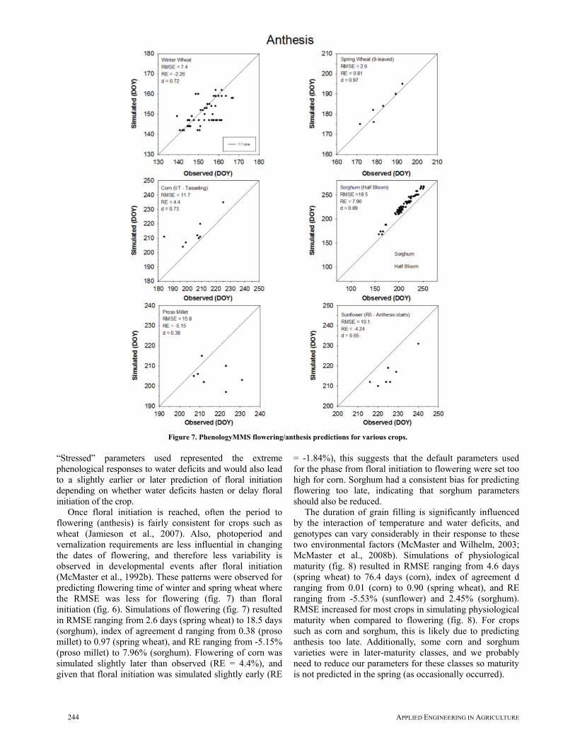
Once floral initiation is reached, often the period to flowering (anthesis) is fairly consistent for crops such as wheat (Jamieson et al., 2007). Also, photoperiod and vernalization requirements are less influential in changing the dates of flowering, and therefore less variability is observed in developmental events after floral initiation (McMaster et al., 1992b). These patterns were observed for predicting flowering time of winter and spring wheat where the RMSE was less for flowering (fig. 7) than floral initiation (fig. 6). Simulations of flowering (fig. 7) resulted in RMSE ranging from 2.6 days (spring wheat) to 18.5 days (sorghum), index of agreement d ranging from 0.38 (proso millet) to 0.97 (spring wheat), and RE ranging from -5.15% (proso millet) to 7.96% (sorghum). Flowering of corn was simulated slightly later than observed (RE = 4.4%), and given that floral initiation was simulated slightly early (RE

= -1.84%), this suggests that the default parameters used for the phase from floral initiation to flowering were set too high for corn. Sorghum had a consistent bias for predicting flowering too late, indicating that sorghum parameters should also be reduced.

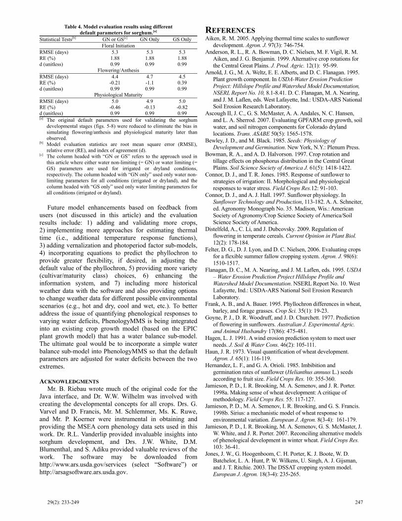
The duration of grain filling is significantly influenced by the interaction of temperature and water deficits, and genotypes can vary considerably in their response to these two environmental factors (McMaster and Wilhelm, 2003; McMaster et al., 2008b). Simulations of physiological maturity (fig. 8) resulted in RMSE ranging from 4.6 days (spring wheat) to 76.4 days (corn), index of agreement d ranging from 0.01 (corn) to 0.90 (spring wheat), and RE ranging from -5.53% (sunflower) and 2.45% (sorghum). RMSE increased for most crops in simulating physiological maturity when compared to flowering (fig. 8). For crops such as corn and sorghum, this is likely due to predicting anthesis too late. Additionally, some corn and sorghum varieties were in later-maturity classes, and we probably need to reduce our parameters for these classes so maturity is not predicted in the spring (as occasionally occurred).

Figure 7. PhenologyMMS flowering/anthesis predictions for various crops.

29(2): 233-249 245

Absolute RE was less than 8% for all crop developmental event simulations, with index of agreement d greater than 0.7 for the majority of simulations. For the emergence and floral initiation developmental event simulations, RMSE was less than 10 days with the exception of floral initiation for winter wheat (RMSE = 12.4 days). Based on the statistical evaluation results, PhenologyMMS simulated the emergence and floral initiation developmental events more accurately than the anthesis and maturity events (where simulation results indicated that the default parameters needed slight adjustment). However, given the limited information for precise determination of initial inputs and based on the model evaluation statistics, we feel that PhenologyMMS demonstrates reasonable accuracy in predicting crop development and therefore the decision tool can be used in a number of applications. One potential application of PhenologyMMS is to conduct simulations using historical weather data at different sites and estimate the mean and range of dates for different developmental events. Therefore, we ran PhenologyMMS for ten locations in the Central Great Plains and focused on the three developmental stages of jointing (near floral initiation), anthesis, and physiological maturity (table 3). Several patterns were observed in this application. First, as expected the mean date of all three developmental events occurred increasingly later as latitude

increased due to slower accumulation of thermal time. The deviation in this trend for the Fort Collins, Colorado location is due to the higher elevation and proximity to the foothills that results in cooler temperatures than found at comparable latitudes to the east (e.g., Akron and Sterling, Colo.). Second, comparing stressed to optimal conditions, the mean date of a developmental stage under stressed conditions occurred increasingly earlier for jointing to anthesis to maturity. Third, typically the range around the mean decreased from jointing to anthesis to maturity for both stressed and optimal conditions. Further applications of PhenologyMMS could explore different possible or projected changes in climate, although particular caution is warranted until photoperiod and vernalization factors are included in the model.

As previously stated, with few exceptions crop phenology simulation models do not consider the influence of water deficits on phenology. To further investigate whether the approach used in PhenologyMMS improved the accuracy of phenological predictions (by incorporating the influence of water deficits), we selected sorghum for further evaluation because a fairly even balance between dryland and irrigated data sets were available. Before beginning the analysis, we reduced the parameters predicting flowering and physiological maturity (figs. 7 and 8) to eliminate the model bias of predicting these

Figure 8. PhenologyMMS physiological maturity predictions for various crops. Two data points for a late-maturing corn hybrid that were simulated to occur in the spring are not shown in the graph to allow easier reading of the graph.

246 APPLIED ENGINEERING IN AGRICULTURE

developmental stages late. PhenologyMMS was then run using different combinations of default parameters for limiting or non-limiting conditions. The first approach was that used in this article where either the parameters for non-limiting (fig. 3d) or water-limiting conditions were selected based on whether the site was irrigated or dryland, respectively (figs. 5-8). The second and third approaches were based on the approach common in plant growth models where a static parameter is used regardless of water deficits. In our case, either the water non-limiting parameters were used for all sites, whether dryland or irrigated, or the water-limiting parameters were used for all sites.

Results of the three sets of runs are presented in table 4. No difference between the sets was found for the developmental stage of floral initiation due to equal thermal time from emergence to floral initiation for both non-limiting and limiting conditions (= 450 GDD for a medium maturity cultivar). Predicting flowering using a mixture of non-limiting and limiting parameters resulted in a lower RMSE (4.4 days) than either using only non-limiting (4.7 days) or limiting parameters (4.5 days), and the RE was also the lowest. Predicting maturity showed no difference in the RMSE (5.0 days) between using a mixture of non-limiting and limiting parameters and using only limiting parameters, although the RE was slightly less when using a mixture (-0.46%) than only limiting (-0.82%) parameters. However, using only non-limiting parameters had the lowest RMSE (4.9 days) and RE (-0.13). Therefore, using a mixture of non-limiting and limiting parameters resulted in more accurate simulation of flowering and maturity than using only limiting parameters. Although using only non-limiting parameters resulted in better prediction of maturity than using a mixture of non-limiting and limiting parameters (RMSE was reduced by 0.1 day

and RE was reduced by 0.33%), the mixture predicted anthesis more accurately than using only non-limiting parameters (RMSE was reduced by 0.3 day and RE was reduced by 0.89%). This suggests there was benefit to the approach being used in PhenologyMMS of having parameters that reflect differences in environmental conditions.

CONCLUSIONS AND FUTURE RESEARCH Modeling of environmental systems is challenging in

part because process interaction often spans several disciplines, making it difficult to model integrated system response. PhenologyMMS is intended to provide a simple and easy to use program to predict and understand crop phenology and how phenology responds to varying water deficits. Version 1.2 largely meets this objective, yet further work is needed as the statistical evaluation results presented herein suggest that the default parameters for certain crops and developmental stages should be adjusted slightly for the developmental events of emergence, floral initiation, flowering, and maturity. To some extent, the evaluation results indicate the degree of accuracy provided by PhenologyMMS (at least for the data sets evaluated). However, it is challenging to extrapolate these results to future PhenologyMMS applications as the model degree of accuracy is almost certainly location/crop dependent and also varies depending on the statistical evaluation criteria of choice. Because of this uncertainty, it is also difficult to explicitly state the PhenologyMMS applications for which a particular degree of simulation accuracy should be expected; however, based on the evaluation results the model should perform within 10-15% RE for multiple locations and crop developmental events.

Table 3. Mean simulated dates and range of days for a “generic” wheat variety to reach certain growth stages under optimal (i.e., irrigated) and stressed conditions (i.e., dryland) for various locations in the Great Plains, USA (adapted from McMaster and Wilhelm, 2010) [a].

Mean Date and Range (number of days) 2 Leaves Jointing Anthesis Maturity

Location/Latitude # years Optimal Optimal Stress Optimal Stress Optimal Stress Durant, Okla./ 33.99° N, 96.37° W

74 30 Sep

(-3 to 4) 9 March

(-24 to 30) 9 March

(-24 to 30) 12 April

(-22 to 24) 8 April

(-21 to 24) 21 May

(-16 to 22) 9 May

(-18 to 20) Walsh, Colo./ 37.39° N, 102.28° W

12 6 Oct

(-5 to 4) 7 April

(-8 to 15) 7 April

(-8 to 14) 14 May

(-11 to 10) 10 May

(-11 to 10) 21 June

(-7 to 8) 9 June

(-9 to 9) Rocky Ford, Colo./ 38.05° N, 103.71° W

28 8 Oct

(-5 to 23) 14 April

(-20 to 14) 14 April

(-21 to 13) 18 May

(-20 to 17) 14 May

(-20 to 13) 25 June

(-15 to 16) 13 June

(-17 to 14) Stratton, Colo./ 39.30° N, 102.60° W

19 8 Oct

(-3 to 4) 21 April

(-10 to 16) 21 April

(-11 to 16) 27 May

(-10 to 11) 23 May

(-10 to 11) 3 July

(-7 to 10) 22 June

(-7 to 10) Colby, Kan./ 39.40° N, 101.05° W

21 8 Oct

(-5 to 9) 18 April

(-17 to 19) 17 April

(-16 to 19) 22 May

(-14 to 14) 18 May

(-13 to 14) 27 June

(-8 to 12) 16 June

(-9 to 13) Akron, Colo./ 40.16° N, 103.21° W

29 10 Oct

(-6 to 11) 28 April

(-19 to 21) 27 April

(-19 to 22) 2 June

(-13 to 14) 29 May

(-15 to 15) 9 July

(-9 to 12) 28 June

(-10 to 12) Fort Collins, Colo./ 40.59° N, 105.08° W

30 14 Oct

(-10 to 10) 1 May

(-24 to 12) 1 May

(-24 to 12) 5 June

(-25 to 8) 1 June

(-25 to 8) 13 July

(-18 to 9) 1 July

(-19 to 9) Sterling, Colo./ 40.63° N, 103.21° W

13 10 Oct

(-5 to 3) 27 Apr

(-11 to 9) 26 Apr

(-10 to 10) 31 May

(-11 to 7) 27 May

(-11 to 7) 7 July

(-8 to 7) 26 June (-9 to 8)

Shelton, Neb./ 40.78° N, 98.73° W

14 9 Oct

(-4 to 4) 27 April

(-12 to 14) 26 April

(-12 to 15) 29 May

(-11 to 11) 25 May

(-11 to 11) 3 July

(-4 to 10) 22 June

(-7 to 10) Sidney, Neb./ 41.14° N, 102.98° W

23 14 Oct

(-7 to 9) 3 May

(-13 to 17) 3 May

(-14 to 16) 6 June

(-14 to 12) 2 June

(-14 to 13) 13 July

(-7 to 9) 2 July

(-8 to 9) [a] Initial inputs assumed a 15 September planting date, optimal soil water at planting (table 2 values), 5-cm seeding depth, and Method 1 for calculating

thermal time with a 0°C base temperature. The number of historical years of weather data used for each location (arranged in order of increasing latitude) are noted.

29(2): 233-249 247

Future model enhancements based on feedback from users (not discussed in this article) and the evaluation results include: 1) adding and validating more crops, 2) implementing more approaches for estimating thermal time (i.e., additional temperature response functions), 3) adding vernalization and photoperiod factor sub-models, 4) incorporating equations to predict the phyllochron to provide greater flexibility, if desired, in adjusting the default value of the phyllochron, 5) providing more variety (cultivar/maturity class) choices, 6) enhancing the information system, and 7) including more historical weather data with the software and also providing options to change weather data for different possible environmental scenarios (e.g., hot and dry, cool and wet, etc.). To better address the issue of quantifying phenological responses to varying water deficits, PhenologyMMS is being integrated into an existing crop growth model (based on the EPIC plant growth model) that has a water balance sub-model. The ultimate goal would be to incorporate a simple water balance sub-model into PhenologyMMS so that the default parameters are adjusted for water deficits between the two extremes.

ACKNOWLEDGMENTS Mr. B. Riebau wrote much of the original code for the

Java interface, and Dr. W.W. Wilhelm was involved with creating the developmental concepts for all crops. Drs. G. Varvel and D. Francis, Mr. M. Schlemmer, Ms. K. Ruwe, and Mr. P. Koerner were instrumental in obtaining and providing the MSEA corn phenology data sets used in this work. Dr. R.L. Vanderlip provided invaluable insights into sorghum development, and Drs. J.W. White, D.M. Blumenthal, and S. Adiku provided valuable reviews of the work. The software may be downloaded from http://www.ars.usda.gov/services (select “Software”) or http://arsagsoftware.ars.usda.gov.

REFERENCES Aiken, R. M. 2005. Applying thermal time scales to sunflower

development. Agron. J. 97(3): 746-754. Anderson, R. L., R. A. Bowman, D. C. Nielsen, M. F. Vigil, R. M.

Aiken, and J. G. Benjamin. 1999. Alternative crop rotations for the Central Great Plains. J. Prod. Agric. 12(1): 95-99.

Arnold, J. G., M. A. Weltz, E. E. Alberts, and D. C. Flanagan. 1995. Plant growth component. In USDA-Water Erosion Prediction Project: Hillslope Profile and Watershed Model Documentation, NSERL Report No. 10, 8.1-8.41. D. C. Flanagan, M. A. Nearing, and J. M. Laflen, eds. West Lafayette, Ind.: USDA-ARS National Soil Erosion Research Laboratory.

Ascough II, J. C., G. S. McMaster, A. A. Andales, N. C. Hansen, and L. A. Sherrod. 2007. Evaluating GPFARM crop growth, soil water, and soil nitrogen components for Colorado dryland locations. Trans. ASABE 50(5): 1565-1578.

Bewley, J. D., and M. Black. 1985. Seeds: Physiology of Development and Germination. New York, N.Y.: Plenum Press.

Bowman, R. A., and A. D. Halvorson. 1997. Crop rotation and tillage effects on phosphorus distribution in the Central Great Plains. Soil Science Society of America J. 61(5): 1418-1422.

Connor, D. J., and T. R. Jones. 1985. Response of sunflower to strategies of irrigation: II. Morphological and physiological responses to water stress. Field Crops Res.12: 91-103.

Connor, D. J., and A. J. Hall. 1997. Sunflower physiology. In Sunflower Technology and Production, 113-182. A. A. Schneiter, ed. Agronomy Monograph No. 35. Madison, Wis.: American Society of Agronomy/Crop Science Society of America/Soil Science Society of America.

Distelfeld, A., C. Li, and J. Dubcovsky. 2009. Regulation of flowering in temperate cereals. Current Opinion in Plant Biol. 12(2): 178-184.

Felter, D. G., D. J. Lyon, and D. C. Nielsen, 2006. Evaluating crops for a flexible summer fallow cropping system. Agron. J. 98(6): 1510-1517.

Flanagan, D. C., M. A. Nearing, and J. M. Laflen, eds. 1995. USDA – Water Erosion Prediction Project Hillslope Profile and Watershed Model Documentation. NSERL Report No. 10. West Lafayette, Ind.: USDA-ARS National Soil Erosion Research Laboratory.

Frank, A. B., and A. Bauer. 1995. Phyllochron differences in wheat, barley, and forage grasses. Crop Sci. 35(1): 19-23.

Goyne, P. J., D. R. Woodruff, and J. D. Churchett. 1977. Prediction of flowering in sunflowers. Australian J. Experimental Agric. and Animal Husbandry 17(86): 475-481.

Hagen, L. J. 1991. A wind erosion prediction system to meet user needs. J. Soil & Water Cons. 46(2): 105-111.

Haun, J. R. 1973. Visual quantification of wheat development. Agron. J. 65(1): 116-119.

Hernandez, L. F., and G. A. Orioli. 1985. Imbibition and germination rates of sunflower (Helianthus annuus L.) seeds according to fruit size. Field Crops Res. 10: 355-360.

Jamieson, P. D., I. R. Brooking, M. A. Semenov, and J. R. Porter. 1998a. Making sense of wheat development: A critique of methodology. Field Crops Res. 55: 117-127.

Jamieson, P. D., M. A. Semenov, I. R. Brooking, and G. S. Francis. 1998b. Sirius: a mechanistic model of wheat response to environmental variation. European J. Agron. 8(3-4): 161-179.

Jamieson, P. D., I. R. Brooking, M. A. Semenov, G. S. McMaster, J. W. White, and J. R. Porter. 2007. Reconciling alternative models of phenological development in winter wheat. Field Crops Res. 103: 36-41.

Jones, J. W., G. Hoogenboom, C. H. Porter, K. J. Boote, W. D. Batchelor, L. A. Hunt, P. W. Wilkens, U. Singh, A. J. Gijsman, and J. T. Ritchie. 2003. The DSSAT cropping system model. European J. Agron. 18(3-4): 235-265.

Table 4. Model evaluation results using different default parameters for sorghum.[a]

Statistical Tests[b] GN or GS[c] GN Only GS Only Floral Initiation

RMSE (days) 5.3 5.3 5.3 RE (%) 1.88 1.88 1.88 d (unitless) 0.99 0.99 0.99

Flowering/Anthesis RMSE (days) 4.4 4.7 4.5 RE (%) -0.21 -1.1 0.39 d (unitless) 0.99 0.99 0.99

Physiological Maturity RMSE (days) 5.0 4.9 5.0 RE (%) -0.46 -0.13 -0.82 d (unitless) 0.99 0.99 0.99 [a] The original default parameters used for validating the sorghum

developmental stages (figs. 5-8) were reduced to eliminate the bias insimulating flowering/anthesis and physiological maturity later thanobserved.

[b] Model evaluation statistics are root mean square error (RMSE),relative error (RE), and index of agreement (d).

[c] The column headed with “GN or GS” refers to the approach used inthis article where either water non-limiting (= GN) or water limiting (=GS) parameters are used for irrigated or dryland conditions,respectively. The column headed with “GN only” used only water non-limiting parameters for all conditions (irrigated or dryland), and the column headed with “GS only” used only water limiting parameters forall conditions (irrigated or dryland).

248 APPLIED ENGINEERING IN AGRICULTURE

Keating, B. A., P. S. Carberry, G. L. Hammer, M. E. Probert, M. J. Robertson, D. Holzworth, N. I. Huth, J. N. G. Hargreaves, H. Meinke, Z. Hochman, G. McLean, K. Verburg, V. Snow, J. P. Dimes, M. Silburn, E. Wang, S. Brown, K. L. Bristow, S. Asseng, S. Chapman, R. L. McCown, D. M. Freebairn, and C. J. Smith. 2003. An overview of APSIM, a model designed for farming systems simulation. European J. Agron. 18(3-4): 267-288.

Kiniry, J. R., J. R. Williams, P. W. Gassman, and P. Debaeke. 1992. A general process-oriented model for two competing plant species. Trans. ASAE 35(3): 801-810.

Large, E. C. 1954. Growth stages in cereals. Illustration of the Feekes scale. Plant Pathology 3(4): 128–129.

Marc, J., and J. H. Palmer. 1981. Photoperiodic sensitivity of inflorescence initiation and development in sunflower. Field Crops Res. 4: 155-164.

McCown, R. L., G. L. Hammer, J. N. G. Hargreaves, D. P. Holzworth, and D. M. Freebairn. 1996. APSIM: A novel software system for model development, model testing and simulation in agricultural systems research. Agric. Systems 50(3): 255-271.

McMaster, G. S. 1997. Phenology, development, and growth of the wheat (Triticum aestivum L.) shoot apex: A review. Advances in Agron. 59: 63-118.

McMaster, G. S. 2005. Phytomers, phyllochrons, phenology and temperate cereal development. J. Agric. Sci. 143(2-3): 137-150.

McMaster, G. S., and D. E. Smika. 1988. Estimation and evaluation of winter wheat phenology in the central Great Plains. Agric. and Forest Meteorology 43(1): 1-18.

McMaster, G. S., and W. W. Wilhelm. 1995. Accuracy of equations predicting the phyllochron of wheat. Crop Sci. 35(1): 30-36.

McMaster, G. S., and W. W. Wilhelm. 1997. Growing degree-days: One equation, two interpretations. Agric. and Forest Meteorology 87(4): 291-300.

McMaster, G. S., and W. W. Wilhelm. 2003. Phenological responses of wheat and barley to water and temperature: Improving simulation models. J. Agric. Sci. 141(2): 129-147.

McMaster, G. S., and W. W. Wilhelm. 2010. The wheat plant: Development, growth, and yield. In Wheat Production and Pest Management for the Great Plains Region, 7-16. F. B. Peairs, ed. Colorado State University Extension XCM235. Fort Collins, Colo.: Colorado State University.

McMaster, G. S., J. A. Morgan, and W. W. Wilhelm. 1992a. Simulating winter wheat spike development and growth. Agric. and Forest Meteorology 60(3-4): 193-220.

McMaster, G. S., W. W. Wilhelm, and J. A. Morgan. 1992b. Simulating winter wheat shoot apex phenology. J. Agric. Sci. 119(1): 1-12.

McMaster, G. S., J. C. Ascough II, G. A. Dunn, M. A. Weltz, M. Shaffer, D. Palic, B. Vandenberg, P. Bartling, D. Edmunds, D. Hoag, and L. R. Ahuja. 2002a. Application and testing of GPFARM: A farm and ranch decision support system for evaluating economic and environmental sustainability of agricultural enterprises. Acta Horticulturea 593: 171-177.

McMaster, G. S., D. B. Palic, and G. H. Dunn. 2002b. Soil management alters seedling emergence and subsequent autumn growth and yield in dryland winter wheat-fallow systems in the Central Great Plains on a clay loam soil. Soil & Tillage Res. 65(2): 193-206.

McMaster, G. S., J. C. Ascough II, M. J. Shaffer, L. A. Deer-Ascough, P. F. Byrne, D. C. Nielsen, S. D. Haley, A. A. Andales, and G. A. Dunn. 2003a. GPFARM plant model parameters: Complications of varieties and the genotype x environment interaction in wheat. Trans. ASAE 46(5): 1337-1346.

McMaster, G. S., W. W. Wilhelm, D. B. Palic, J. R. Porter, and P. D. Jamieson. 2003b. Spring wheat leaf appearance and temperature: Extending the paradigm? Annals of Botany 91(6): 697-705.

McMaster, G. S., W. W. Wilhelm, and A. B. Frank. 2005. Developmental sequences for simulating crop phenology for water-limiting conditions. Australian J. Agric. Res. 56(11): 1277-1288.

McMaster, G. S., J. W. White, L. A. Hunt, P. D. Jamieson, S. S. Dhillon, and J. I. Ortiz-Monasterio. 2008a. Simulating the influence of vernalization, photoperiod, and optimum temperature on wheat developmental rates. Annals of Botany 102(4): 561-569.

McMaster, G. S., J. W. White, W. W. Wilhelm, P. D. Jamieson, P. S. Baenziger, A. Weiss, and J. R. Porter. 2008b. Simulating crop phenological responses to water deficits. In Response of Crops to Limited Water: Understanding and Modeling Water Stress Effects on Plant Growth Processes (Advances in Agricultural Systems Research, Synthesis, and Applications: Trans-disciplinary Research, Synthesis, and Applications), 277-300. Vol. 1. L. R. Ahuja, V. R. Reddy, S. A. Anapalli, and Q. Yu, eds. Madison, Wis.: ASA-SSSA-CSSA.

McMaster, G. S., D. A. Edmunds, W. W. Wilhelm, D. C. Nielsen, P. V. V. Prasad, and J. C. Ascough II. 2011. PhenologyMMS: A program to simulate crop phenological responses to water stress. Computers and Electronics in Agric. 77(1): 118-125.

McMaster, G. S., T. R. Green, R. H. Erskine, D. A. Edmunds, and J. C. Ascough II. 2012. Spatial interrelationships between wheat phenology, thermal time, and terrain attributes. Agron. J. 104(4): 1110-1121.

McMaster, G. S., J. C. Ascough II, D. A. Edmunds, L. E. Wagner, F. A. Fox, K. C. DeJonge, and N. C. Hansen. 2013 Simulating unstressed crop development and growth using the Unified Plant Growth Model (UPGM). Environmental Modeling & Assessment (In review).

Moragues, M., and G. S. McMaster. 2011. Crop development related to temperature and photoperiod in temperate cereals. In Encyclopedia of Sustainability Science and Technology. R. A. Meyers, ed. Heidelberg, Germany: Springer-Verlag. Available at: www.springerreference.com/docs/html/chapterdbid/226420.html.

Nielsen, D. C., M. F. Vigil, and J. G. Benjamin. 2006. Forage yield response to water use for dryland corn, millet, and triticale in the Central Great Plains. Agron. J. 98(4): 992-998.

Porter, J. R. 1984. A model of canopy development in winter wheat. J. Agric. Sci. 102(2): 383-392.

Porter, J. R. 1993. AFRCWHEAT2: A model of the growth and development of wheat incorporating responses to water and nitrogen. European J. Agron. 2: 64-77.

Rickman, R. W., and B. Klepper. 1995. The phyllochron: Where do we go in the future? Crop Sci. 35(1): 44-49.

Ritchie, S. W., J. J. Hanway, and G. O. Benson. 1986. How a Corn Plant Develops. Iowa State Univ. Coop. Ext. Spec. Rep. No. 48 (revised). Ames, Iowa: Iowa State Univ.

Schaffer, J. A. 1980. The effect of planting date and environment on the phenology and modeling of grain sorghum, Sorghum bicolor (L.) Moench. PhD diss. Manhattan, Kan.: Department of Agronomy, Kansas State University.

Schneiter, A. A. 1994. Introduction. In Sunflower Production. D. R. Berglund, ed. North Dakota State Univ. Ext. Bull. 25 (revised). Fargo, N.D.: North Dakota State Univ.

Schneiter, A. A., ed. 1997. Sunflower Technology and Production. Madison, Wis.: American Society of Agronomy/Crop Science Society of America/Soil Science Society of America.

Schneiter, A. A., and J. F. Miller. 1981. Description of sunflower growth stages. Crop Sci. 21(6): 901-903.

Schneiter, A. A., J. F. Miller, and D. R. Berglund. 1998. Stages of sunflower development. North Dakota State University Extension Service Publication A-1145. Available at: www.ag.ndsu.edu/pubs/plantsci/rowcrops/a1145.pdf. Accessed 3 November 2012.

29(2): 233-249 249

Streck, N. A., A. Weiss, Q. Xue, and P. S. Baenziger. 2003. Incorporating a chronology response into the prediction of leaf appearance rate in winter wheat. Annals of Botany 92(2): 181-190.

Unger, P. W. 1983. Irrigation effect on sunflower growth, development, and water use. Field Crops Res. 7: 181-194.

Wagner, L. E. 1996. An overview of the wind erosion prediction system. In Proc. Intl. Conf. on Air Pollution from Agricultural Operations, 73-75. Ames, Iowa: Midwest Plan Service.

Waldren, R. P., and A. D. Flowerday. 1979. Growth stages and distribution of dry matter, N, P, and K in winter wheat. Agron. J. 71(3): 391-397.

Weir, A. H., P. L. Bragg, J. R. Porter, and J. H. Rayner. 1984. A winter wheat crop simulation model without water or nutrient limitations. J. Agric. Sci. 102(2): 371-382.

White, J. W., M. Herndl, L. A. Hunt, T. S. Payne, and G. Hoogenboom. 2008. Simulation-based analysis of effect of Vrn and Ppd loci on flowering in wheat. Crop Sci. 48(2): 678-687.

Wilhelm, W. W., G. S. McMaster, R. W. Rickman, and B. Klepper. 1993. Above-ground vegetative development and growth of winter wheat as influenced by nitrogen and water availability. Ecological Modelling 68(3-4): 183-203.

Wilhelm, W. W., G. E. Varvel, and J. S. Scheppers. 2005. Corn stalk nitrate concentration profile. Agron. J. 97(6): 1502-1507.

Williams, J. R., C. A. Jones, J. R. Kiniry, and D. A. Spanel. 1989. The EPIC crop growth model. Trans. ASAE 32(2): 497-511.

Yan, W., and L. A. Hunt. 1999. An equation for modelling the temperature response of plants using only the cardinal temperatures. Annals of Botany 84(5): 607-614.

Yegappan, T. M., D. B. Paton, C. T. Gates, and W. J. Muller. 1980. Water stress in sunflower (Helianthus annuus L.): I. Effect on plant development. Annals of Botany 46(1): 61-70.

Zadoks, J. C., T. T. Chang, and C. F. Konzak. 1974. A decimal code for the growth stages of cereals. Weed Res. 14(6): 415-421.

Zalud, Z., G. S. McMaster, and W. W. Wilhelm. 2003. Evaluating SHOOTGRO 4.0 as a potential winter wheat management tool in the Czech Republic. European J. Agron. 19(4): 495-507.