Date:

Leibniz Centre for Agricultural Landscape Research (ZALF)

Simulating crop canopy temperature

Heidi Webber, Jeff White, Bruce Kimball, Frank Ewert,Senthold Asseng, Ehsan Rezaei, Jim Pinter, JerryHatfield, Matthew Reynolds, Behnam Ababaei,,Marco Bindi, Jordi Doltra, Roberto Ferrise, HenningKage, Belai Kassie, KC Kersebaum, Adam Luig,Jorgen Olesen, Micha Semenov, PierreStratonovitch, Arne Ratjen, Robert LaMorte, StephenLeavitt, Doug Hunsaker, Gerard Wall, Pierre Martre

19.10.2020

Temperature impacts on global crop yields

Grain yield changes (%) with 1 °C increase

(Zhao et al, 2017)

Which temperature should be used to assess temperature effects?

How different are air and crop temperatures?

(Prasher and Jones, 2014)- plots have same air temperature recorded at weather station- air temperature can not distinguish irrigated and rainfed plots

• Cooler canopies under heat & drought stress correlate with higher yields

• Indirect indicator of water use• Modelling could allow to test GxE:

WSC vs deeper roots?

Wheat grain yield response to crop temperature

(Lopes and Reynolds, 2010)

2007

2008

Indicator of heat & drought resistance

Crop temperature better explains current yield variability

Spanish irrigated maize (1982 – 2014)

(Siebert et al., 2017)

Tair

Tc

Error in simulated heat stress under climate change

Change in heat stress

Tair Tc ΔYTair - Δ YTcan

ΔY difference

Irrigated maize (2080, RCP8.5, HadGEM2-ES)

(Siebert et al., 2017)

How to account for in crop models?

𝛾∗ = 𝛾 1 + &𝑟( 𝑟)

𝑇( = 𝑇) +𝑅, − 𝐺

𝜌𝑐1𝛾∗

∆ + 𝛾∗𝑟) −

𝑉𝑃𝐷∆ + 𝛾∗

Canopy resistance (CO2, water, nitrogen, …)

Evaporative cooling

Aerodynamic resistance𝑟) = 𝑓 𝑤𝑖𝑛𝑑, ℎ𝑒𝑖𝑔ℎ𝑡, 𝐿𝐴𝐼, 𝑠𝑡𝑎𝑏𝑖𝑙𝑖𝑡𝑦 = 𝑓 𝑇(

Radiative heatingAir temp

Highly non-linear, analytical solution not possible

….complexity makes a case for RS data for calibration

1. Energy balance with stability corrections (EBSC)2. Energy balance with neutral stability (EBN)3. Empirical (EMP)

Approaches to simulate canopy temperature

• Empirical approaches did very well• Little improvement in yield simulation with Tc

• Good yield simulation with poor Tc sims

Reflect on models & test for more conditions

CW (Reginato et al, 1988)– 2-years, 2-water – non-limiting N– Dataset is 30-

years old, many uncertainties

– Has Ta > 31°C at 3-sites

FACE (Kimball et al, 1996, 2000)– 4-years – 2 – [CO2], 2-N & 2-

irrigation– Minimal Ta > 31°

2017

2018

9Results

Correlation across production conditions and CO2

Tc model

type

CW Water FACE Water FACE Nitrogen FACE CO2

Model Irr Rain Full Irr Semi Irr High Low Amb Elev

REF-E HU 0.40 0.48 0.52 0.22 0.51 0.45 0.51 0.53

EMP DN 0.27 0.14 0.31 - 0.23 0.28 0.24 0.24

EMP FA 0.20 0.12 0.12 0.15 0.25 - 0.19 0.17

EBN HE 0.14 - 0.25 0.04 0.27 0.25 0.20 0.22

EBN SQ 0.16 - 0.32 0.08 0.27 0.21 0.24 0.27

EBN SS - 0.10 0.28 0.13 0.29 0.22 0.28 0.26

EBN S2 0.13 - 0.03 - 0.07 - 0.08 0.04

EBSC L5 0.27 0.27 0.49 0.03 0.34 0.51 0.34 0.32

EBSC SP 0.41 0.30 0.36 0.13 0.37 0.31 0.37 0.34

# obs 53 52 357 122 368 110 239 240

1- EBSC best; 2- variation within types

10Results

Where do the models succeed and fail?

Type 1 Sequential Sums of Squares (% of total variation)

Very large residuals… What is going on the with data?

FACE China Wheat

11Results

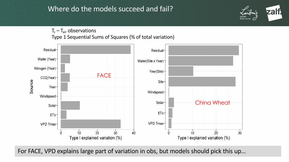
Where do the models succeed and fail?

Tc – Tair observationsType 1 Sequential Sums of Squares (% of total variation)

For FACE, VPD explains large part of variation in obs, but models should pick this up…

FACE

China Wheat

12CT2: Results

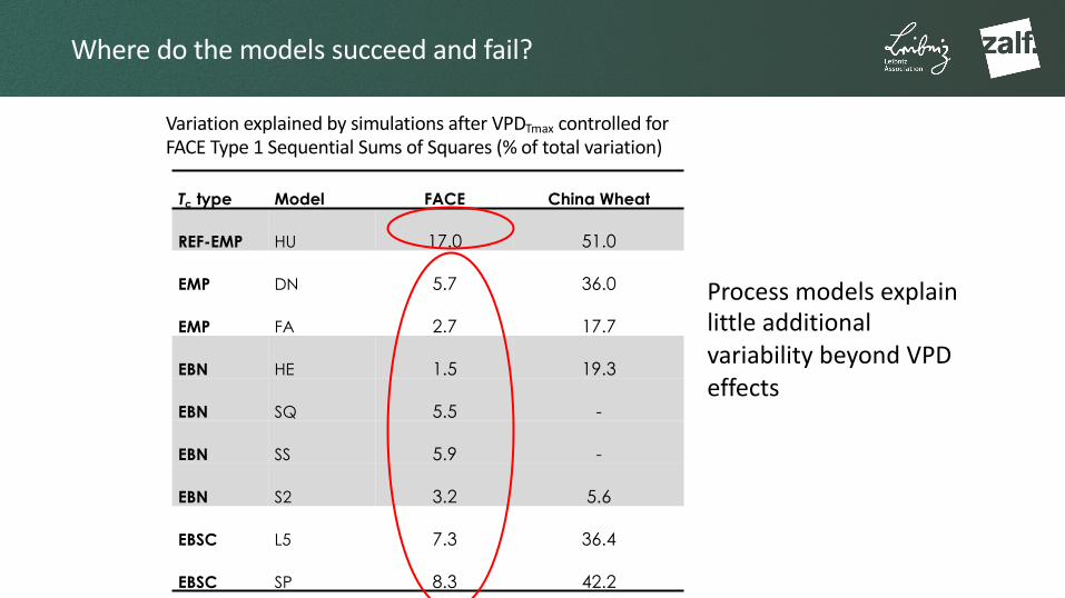
Where do the models succeed and fail?

Variation explained by simulations after VPDTmax controlled forFACE Type 1 Sequential Sums of Squares (% of total variation)

Process models explain little additional variability beyond VPD effects

Tc type Model FACE China Wheat

REF-EMP HU 17.0 51.0

EMP DN 5.7 36.0

EMP FA 2.7 17.7

EBN HE 1.5 19.3

EBN SQ 5.5 -

EBN SS 5.9 -

EBN S2 3.2 5.6

EBSC L5 7.3 36.4

EBSC SP 8.3 42.2

13

Where do the models succeed and fail?

Response to CO2 over all observations

14Summary

Summary

§ Models explain up to 50% of variation in observations § Stability correction improves model skill § Each type could explain CO2

Next steps§ Understand cause of high residual error (Jeff White)§ Need for high volume, high quality datasets

§ Improve ET simulations§ Extend to all growth processes§ 2 source energy balance

§ Distinguish varietal differences§ Develop hybrid RS & crop models combinations to allow less intrusive

quantification of crop water use