Simulated and experimental results on heat recovery from hot steel beams in a cooling bed applying modified solar absorbers

Joana Tarrésa*P, Stefan Maasa, Frank Scholzena, Arno Zürbesb,

a Faculty of Science, Technology and Communication. University of Luxembourg. 6, Rue de Coudenhove Kalergi. 1359 Luxembourg. Luxembourg

b Fachhochschule Bingen. Berlinstras. 109. 5541 Bingen, Germany

*Corresponding author: Tel: +352 466644 5222. Fax: +352 466644 5200 Email address: ; joana.tarres@uni.lu, joana.tarres@gmail.com

ABSTRACT1

In recent years, the steel industry has undertaken efforts to increase energy efficiency by reducing energy consumption and recover otherwise lost heat. About 60% of the energy consumed in a steel plant is lost in cooling beds where the hot steel beams are cooled down by natural convection and radiation. In this paper, the potential of heat recovery by radiation in a cooling bed was determined. Firstly, numerical simulations of the heat flux were done and validated with experimental measures. Secondly, a pilot test to recover the heat with modified solar absorbers was installed at the side of the cooling bed. The standard solar panels were painted with high absorption paint in the wavelength range of the hot beams. The results showed that up to 1 kW/m2 could be recovered with a temperature of 70°C at the side of the cooling bed, with a thermal efficiency of approximately 40%. As the experimental results were promising, further research is suggested to find an adequate selective coating and glazing. This would maximize the absorption at the wavelength range of the hot beams and minimize the emissivity at operational temperature of the absorber (100°C). Additionally, it would be of interest to find the optimum position for the absorbers in the cooling bed, which maximizes the heat recovery and does not interfere in the production process.

KEYWORDS: heat recovery, solar absorbers, steel production, cooling bed, steel beams, thermal solar technology, radiation, heat transfer, wavelength

1. Introduction

The iron and steel industry is an intensive energy consumer. In Europe it uses 19% of the final energy consumed in industry (Eurostat, 2009). In recent years, the iron and steel industry has

1 Abbreviations : NIR; Near infrared; MIR, Mid infrared; FIR, Far infrared; DAQ, data acquisition system; IR, Infrared; PVD, Physical Vapor Deposition; CSP,Concentrating Solar Panel; DM, double meander; BC, black chrome, HP, Harp absorber; ORC, Organic Rankine Cycle

1

done efforts to reduce the energy consumption and to recover otherwise lost heat. Some of the technologies under research can have an important impact to the reduction of CO2 emissions in European industry, according to the bottom up model presented by Moya and Pardo (Moya and Pardo, 2013).

The production of steel is divided in integrated steelmaking and electric steelmaking. The first route produces steel from iron ore in blast furnaces and in the second route an electric arc furnace melts scrap. The integrated steelmaking route consumes five times the primary energy consumed for electric steelmaking according to Kirschen (Kirschen et al., 2009).

This paper is focusing in a Luxembourgish electric steel plant. An energy audit was established in order to identify the main waste heat sources. The main energy consumers are the furnaces: the electric arc furnace to melt the steel and the two reheating furnaces to reheat the semi-finished products (beam blanks) before milling. Approximately 60% of the energy used to heat up the steel is lost in three cooling beds in the steel plant (Tarres Font et al., 2011).

In literature there are several references about waste heat recovery in steel industry especially for high and medium grade waste heat. However the rate of recuperation is only 2% for low grade waste heat (temperatures below 150°C) according to Ma (Ma et al., 2012). Several authors highlight the potential of recovering low grade residual energy by technologies like Organic Rankine Cycle (ORC), thermophotovoltaics, heat pipes and thermoelectric technology among others. The captured heat recovered can be used for electricity generation, heating and cooling in the same industry or in the surroundings (Ammar et al., 2012), (Andrews and Pearce, 2011), (Dong et al., 2013).

However not many references have been found regarding the recovery of heat lost in cooling beds. One experience is described in a report from the Iron Office Research of Sweden (Jernkontorets Forskning). Experiments in two cooling beds were conducted by Nilsson (Nilsson, 2003), involving recovery of convective and radiant heat by means of a hoover and solar collectors recovering up to 3 kWh/t. These experiments were mentioned as well by Johansson (Johansson and Söderström, 2011) and Broberg Viklund (Broberg Viklund and Johansson, 2014).

The possibility to use solar panels to recover the heat lost in the cooling bed is analysed in this paper, focusing in a Luxembourgish steel plant. The challenge is to adapt a standard solar absorber to the near and mid infrared radiation emitted by the hot steel beams. It has to be considered that standard solar absorbers have a low reflection at wavelengths below 3μm and high reflection above this value, being thatthe main characteristic of spectrally selective surfaces (Kennedy, 2002).

In a first step the radiation flux available around the cooling bed was simulated together with the emission wavelength . In a second step, a heat recovery pilot test was installed. It consisted of a solar panel with a closed water circuit..

2

Along this paper the simulations, tests and measurement methodologies are described, as well as the results obtained and the possible full scale application. The objective is to determine the amount of heat which can be recovered with solar panels from cooling beds, as well as to identify the achievable temperature and analyze possible usage.

2. Simulations

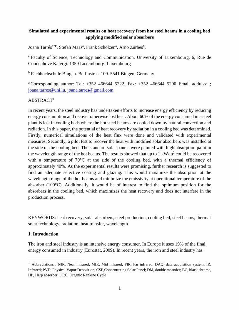
The cooling bed under study cools down steel beams from 800°C to 80°C in approximately 80 min, as can be seen in Figure 1. During the first eight minutes, the beam loses 300°C, approximately 35°C per minute. The heat lost is approximately 91 GWh/y.

The cooling bed is placed after the rolling mill.The rolling mill rolls beams double T, U and angle profiles from 100 to 550 mm height. Once cooled down, the beams pass through a straightening machine before they are cut to the required lengths. The dimensions of the cooling bed are 106 m x 23 m. The cooling of the beams is done by natural convection. The hot beam enters the cooling bed and it is displaced laterally until it reaches the exit roll. Every time a new beam enters, displacement takes place in the cooling bed.

Figure 1: Measured decrease of the steel surface temperature in the cooling bed for different profiles

A model to simulate the heat flux between the hot steel beams in the cooling bed and solar absorbers placed at different positions around the cooling bed was created using MATLAB.

The model was based in the situation represented in Figure 2 and Figure 3. The emitting bodies considered were the first five beams of the cooling bed, corresponding to approximately the first ten minutes from 800°C to 500°C (Figure 1). The distance between beams varies according the profile. The simulated receiving surface was a solar panel of area 1 m2. The solar panels were simulated in different locations: at the hot side of the cooling bed, at the top of the cooling bed

0

100

200

300

400

500

600

700

800

900

1000

0 20 40 60 80

Stee

l bea

m te

mpe

ratu

re [°

C]

Time [min]

3

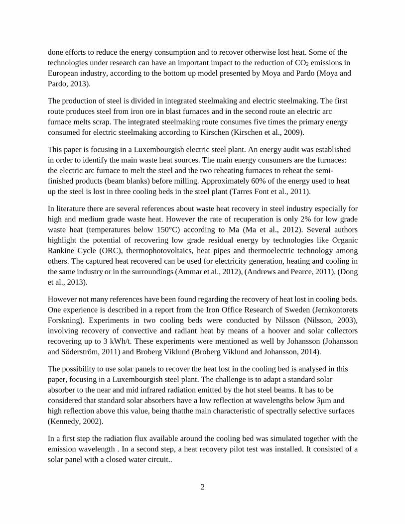
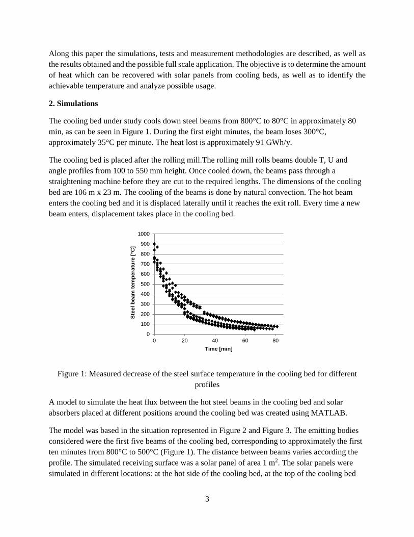
and at the arc surrounding the first beam. For the first case, four different heights and nine angular variations of α=0° till α=80° were simulated (Figure 2). For the second and third case five different heights were assumed and angular variation of σ=10° were considered in the arc (Figure 3).

Figure 2: Scheme of the cooling bed and the solar panels next to the column (distances in mm)

Figure 3: Scheme of the cooling bed and the solar panels at the top and at the arc of the first beam

In order to determine the temperature of the simulated panels, a set of temperature sensors attached to steel plates were installed at the side of the cooling bed. The registers obtained as well as the ambient temperature inside and outside the hall were inputs for the heat flux simulations. .

4

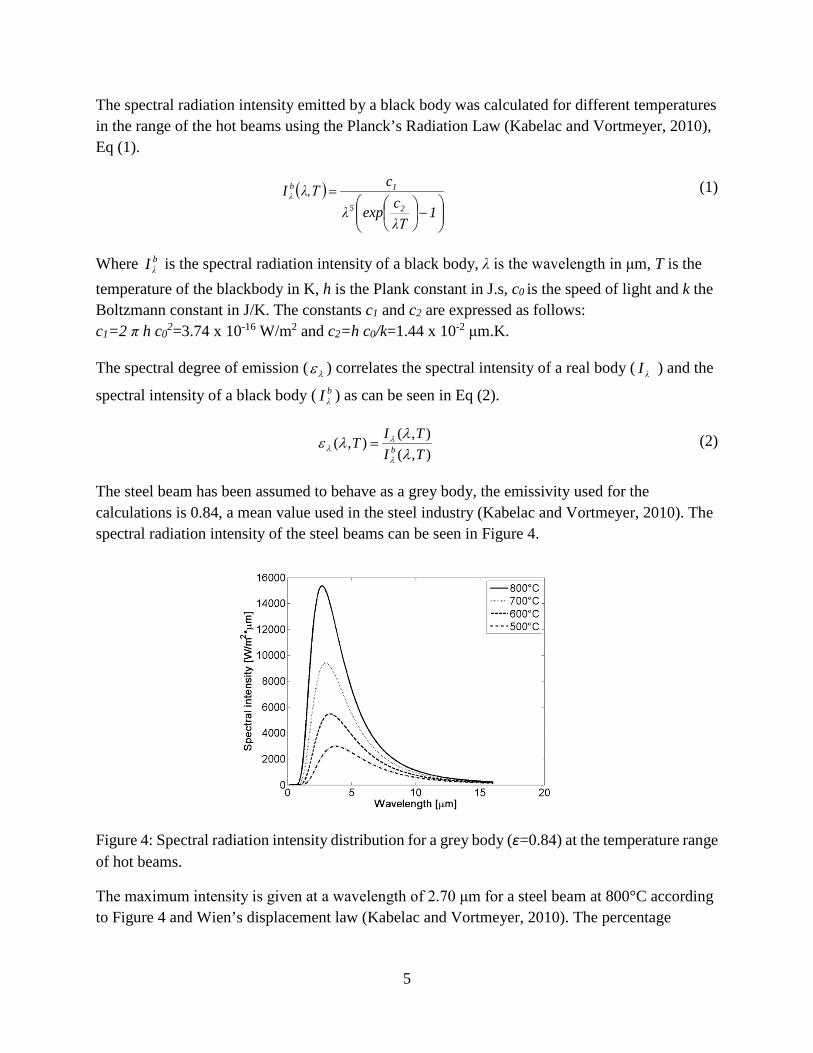
The spectral radiation intensity emitted by a black body was calculated for different temperatures in the range of the hot beams using the Planck’s Radiation Law (Kabelac and Vortmeyer, 2010), Eq (1).

( )

−

=1

λTcexpλ

cλ,TI25

1bλ

(1)

Where bλI is the spectral radiation intensity of a black body, λ is the wavelength in μm, T is the

temperature of the blackbody in K, h is the Plank constant in J.s, c0 is the speed of light and k the Boltzmann constant in J/K. The constants c1 and c2 are expressed as follows: c1=2 π h c0

2=3.74 x 10-16 W/m2 and c2=h c0/k=1.44 x 10-2 μm.K.

The spectral degree of emission ( λε ) correlates the spectral intensity of a real body ( λI ) and the

spectral intensity of a black body ( bλI ) as can be seen in Eq (2).

),(),(),(

TITIT b λ

λλε

λ

λλ = (2)

The steel beam has been assumed to behave as a grey body, the emissivity used for the calculations is 0.84, a mean value used in the steel industry (Kabelac and Vortmeyer, 2010). The spectral radiation intensity of the steel beams can be seen in Figure 4.

Figure 4: Spectral radiation intensity distribution for a grey body (ε=0.84) at the temperature range of hot beams.

The maximum intensity is given at a wavelength of 2.70 μm for a steel beam at 800°C according to Figure 4 and Wien’s displacement law (Kabelac and Vortmeyer, 2010). The percentage

5

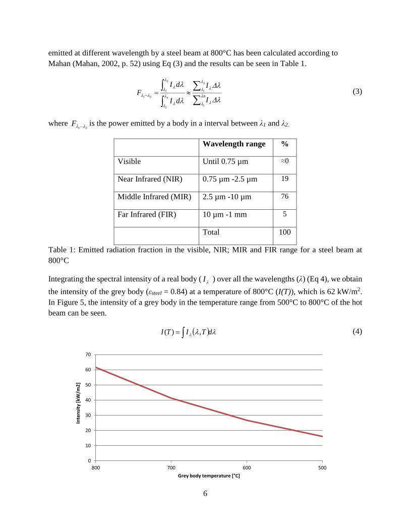
emitted at different wavelength by a steel beam at 800°C has been calculated according to Mahan (Mahan, 2002, p. 52) using Eq (3) and the results can be seen in Table 1.

∑∑

∫∫

≈=− nI

I

dI

dIF

n λ

λ λ

λ

λ λ

λ

λ λ

λ

λ λ

λλλ∆

λ∆

λ

λ

1

2

1

1

2

1

21 (3)

where 21 λλ −F is the power emitted by a body in a interval between λ1 and λ2.

Wavelength range %

Visible Until 0.75 µm ≈0

Near Infrared (NIR) 0.75 µm -2.5 µm 19

Middle Infrared (MIR) 2.5 µm -10 µm 76

Far Infrared (FIR) 10 µm -1 mm 5

Total 100

Table 1: Emitted radiation fraction in the visible, NIR; MIR and FIR range for a steel beam at 800°C

Integrating the spectral intensity of a real body ( λI ) over all the wavelengths (λ) (Eq 4), we obtain the intensity of the grey body (εsteel = 0.84) at a temperature of 800°C (I(T)), which is 62 kW/m2. In Figure 5, the intensity of a grey body in the temperature range from 500°C to 800°C of the hot beam can be seen.

( ) λλλ dTITI ∫= ,)( (4)

0

10

20

30

40

50

60

70

500600700800

Inte

nsity

[kW

/m2]

Grey body temperature [°C]

6

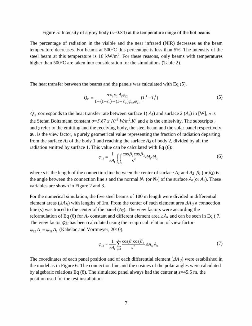
Figure 5: Intensity of a grey body (ε=0.84) at the temperature range of the hot beams

The percentage of radiation in the visible and the near infrared (NIR) decreases as the beam temperature decreases. For beams at 500°C this percentage is less than 5%. The intensity of the steel beam at this temperature is 16 kW/m2. For these reasons, only beams with temperatures higher than 500°C are taken into consideration for the simulations (Table 2).

The heat transfer between the beams and the panels was calculated with Eq (5).

)()1()1(1

42

41

211221

1212112 TTAQ −

−−−−=

ϕϕεεϕεεσ (5)

12Q corresponds to the heat transfer rate between surface 1( A1) and surface 2 (A2) in [W], σ is the Stefan Boltzmann constant σ=5.67 x 10-8 W/m2.K4 and ε is the emissivity. The subscripts 1 and 2 refer to the emitting and the receiving body, the steel beam and the solar panel respectively. φ12 is the view factor, a purely geometrical value representing the fraction of radiation departing from the surface A1 of the body 1 and reaching the surface A2 of body 2, divided by all the radiation emitted by surface 1. This value can be calculated with Eq (6):

21221

112

1 2

coscos1 dAdAsA A A

∫ ∫=ββ

πϕ (6)

where s is the length of the connection line between the center of surface A1 and A2. β1 (or β2) is the angle between the connection line s and the normal N1 (or N2) of the surface A1(or A2). These variables are shown in Figure 2 and 3.

For the numerical simulation, the five steel beams of 100 m length were divided in differential element areas (ΔA1j) with lengths of 1m. From the center of each element area ΔA1j a connection line (s) was traced to the center of the panel (A2). The view factors were according the reformulation of Eq (6) for A2 constant and different element area ΔA1 and can be seen in Eq ( 7. The view factor φ21 has been calculated using the reciprocal relation of view factors

221112 AA ϕϕ = (Kabelac and Vortmeyer, 2010).

∑=

≈n

jj AA

sA 1212

21

112

coscos1 ∆ββπ

ϕ (7)

The coordinates of each panel position and of each differential element (ΔA1j) were established in the model as in Figure 6. The connection line and the cosines of the polar angles were calculated by algebraic relations Eq (8). The simulated panel always had the center at z=45.5 m, the position used for the test installation.

7

sNsN

1

11cos =β (8)

Figure 6: Geometrical representation and coordinate system used for the simulation

The temperatures of the beams used for simulations can be found in table 2. The emissivity of the steel considered was ε1 =0.84 and the emissivity of the panel ε2 =0.94.

Beam number 1 2 3 4 5

Time in the cooling bed min 0 2 4 6 8

Temperature °C 800 730 660 590 520

Table 2: Beam temperature used in simulations

To simplify the calculations, the beams have been assumed to be a rectangular box of H x B dimensions instead of having the real H or I shape of the profile (Figure 6). For each beam the energy emitted for surface H and surface B has been analyzed separately as the view factors vary accordingly. Each connecting line between a beam side and a panel is checked automatically to see if it interferes with another beam. If it does so, the heat flux exchange between this beam side and the panel is not considered. The heat transfer between each beam side interacting with the same panel is summed to find the total heat transfer received by the panel.

3. Experimental pilot test

A pilot test to recover the radiation heat lost by the steel beams was designed with standard equipment for thermal solar installations. The system composed of two closed water circuits. In the first circuit the water heated in the absorbers and exchanged its heat in a water tank. The circuit was driven by a pump with three speeds. The water in the tank circulated in a second

8

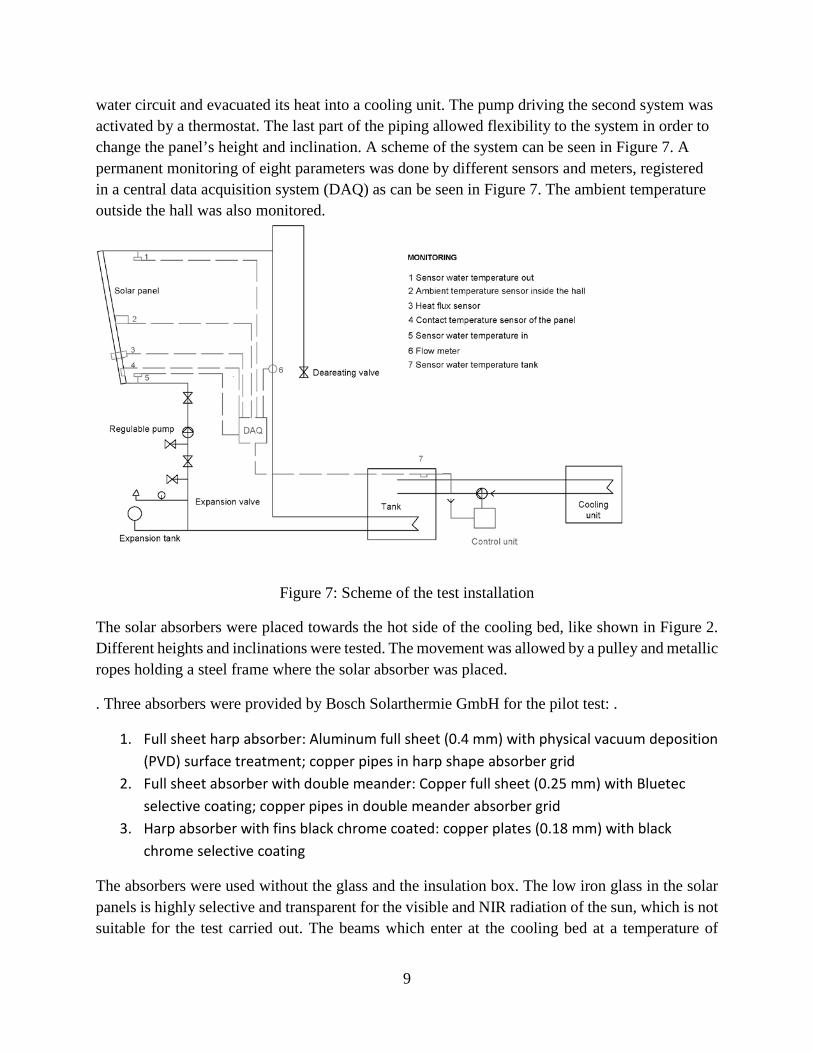
water circuit and evacuated its heat into a cooling unit. The pump driving the second system was activated by a thermostat. The last part of the piping allowed flexibility to the system in order to change the panel’s height and inclination. A scheme of the system can be seen in Figure 7. A permanent monitoring of eight parameters was done by different sensors and meters, registered in a central data acquisition system (DAQ) as can be seen in Figure 7. The ambient temperature outside the hall was also monitored.

Figure 7: Scheme of the test installation

The solar absorbers were placed towards the hot side of the cooling bed, like shown in Figure 2. Different heights and inclinations were tested. The movement was allowed by a pulley and metallic ropes holding a steel frame where the solar absorber was placed.

. Three absorbers were provided by Bosch Solarthermie GmbH for the pilot test: .

1. Full sheet harp absorber: Aluminum full sheet (0.4 mm) with physical vacuum deposition (PVD) surface treatment; copper pipes in harp shape absorber grid

2. Full sheet absorber with double meander: Copper full sheet (0.25 mm) with Bluetec selective coating; copper pipes in double meander absorber grid

3. Harp absorber with fins black chrome coated: copper plates (0.18 mm) with black chrome selective coating

The absorbers were used without the glass and the insulation box. The low iron glass in the solar panels is highly selective and transparent for the visible and NIR radiation of the sun, which is not suitable for the test carried out. The beams which enter at the cooling bed at a temperature of

9

approximate 800°C have a maximum of emission at a wavelength of 2.7 µm and only 19% is emitted in the NIR wavelengths (Table 1). Hence the low iron glass would reflect most of the incident radiation. The absorber was insulated at the back side by a box of rock wool and placed in a steel frame for the test purposes.

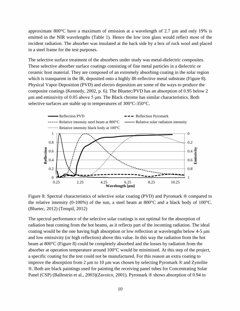
The selective surface treatment of the absorbers under study was metal-dielectric composites. These selective absorber surface coatings consisting of fine metal particles in a dielectric or ceramic host material. They are composed of an extremely absorbing coating in the solar region which is transparent in the IR, deposited onto a highly IR-reflective metal substrate (Figure 8). Physical Vapor Deposition (PVD) and electro deposition are some of the ways to produce the composite coatings (Kennedy, 2002, p. 6). The Bluetec/PVD has an absorption of 0.95 below 2 μm and emissivity of 0.05 above 5 μm. The Black chrome has similar characteristics. Both selective surfaces are stable up to temperatures of 300°C-350°C.

Figure 8: Spectral characteristics of selective solar coating (PVD) and Pyromark ® compared to the relative intensity (0-100%) of the sun, a steel beam at 800°C and a black body of 100°C. (Bluetec, 2012) (Tempil, 2012)

The spectral performance of the selective solar coatings is not optimal for the absorption of radiation heat coming from the hot beams, as it reflects part of the incoming radiation. The ideal coating would be the one having high absorption or low reflection at wavelengths below 4-5 μm and low emissivity (or high reflection) above this value. In this way the radiation from the hot beam at 800°C (Figure 8) could be completely absorbed and the losses by radiation from the absorber at operation temperature around 100°C would be minimized. At this step of the project, a specific coating for the test could not be manufactured. For this reason an extra coating to improve the absorption from 2 μm to 10 μm was chosen by selecting Pyromark ® and Zynolite ®. Both are black paintings used for painting the receiving panel tubes for Concentrating Solar Panel (CSP) (Ballestrin et al., 2003)(Zavoico, 2001). Pyromark ® shows absorption of 0.94 in

0

0.2

0.4

0.6

0.8

10

0.2

0.4

0.6

0.8

1

0.25 2.25 4.25 6.25 8.25 10.25

Emiss

ivity

Ref

lect

ion

Wavelength [μm]

Reflection PVD Reflection PyromarkRelative intensity steel beam at 800°C Relative solar radiation intensityRelative intensity black body at 100°C

10

wavelengths from 0.3 to 26 μm, as can be seen in Figure 8. The absorption is very high for the wavelengths in the infrared, which makes it suitable to absorb the heat from the hot beams. However, the thermal losses of the panel at 100°C will not be reduced with Pyromark ®, as it is not selective.

The heat recovered by the collector can be described using Eq (9) according to Foster (Foster et al., 2009), not considering the losses by radiation:

)(0 aminu TTUqq −−= η (9)

Where uq is the heat recovered by the collector in W/m2, inq is the incoming heat flux on collector plane in W/m2, the 0η is the optical efficiency and U is the overall heat loss coefficient due to convection and conduction (W/m2.K). Ta refers to ambient temperature and Tm is the mean collector temperature defined as Tm=(Tout-Tin)/2, where Tout and Tin are the water temperature out and in of the panel. The efficiency of the panel is:

in

aminu q

TTUqq

)(/ 0

−−== ηη (10)

The heat recovered by the panel was measured experimentally according Eq (11).

)( inoutpu TTcmqw

−= ∫ (11)

Where m is the mass flow in kg/s, wpc is the specific heat of water

wpc = 4.18 kJ/kg.K. Tout and

Tin are the water temperature out and in of the panel measured by the temperature sensors 1 and 5 in Figure 7.

4. Simulation results

The temperature registered in the preliminary sensors at the side of the cooling bed oscillated between 100°C and 140°C at 4.5 m. Stops in the mill due to change of the profile or technical problems were reflected in the temperature measurement. The usual stops were lasting from 2 min till 40 min. The temperature decreased 80°C in 20 minutes. The data registered has been cross checked with the production data showing changes in the temperature registered according to the profile milled. The bigger the profile, the higher the temperature registered.

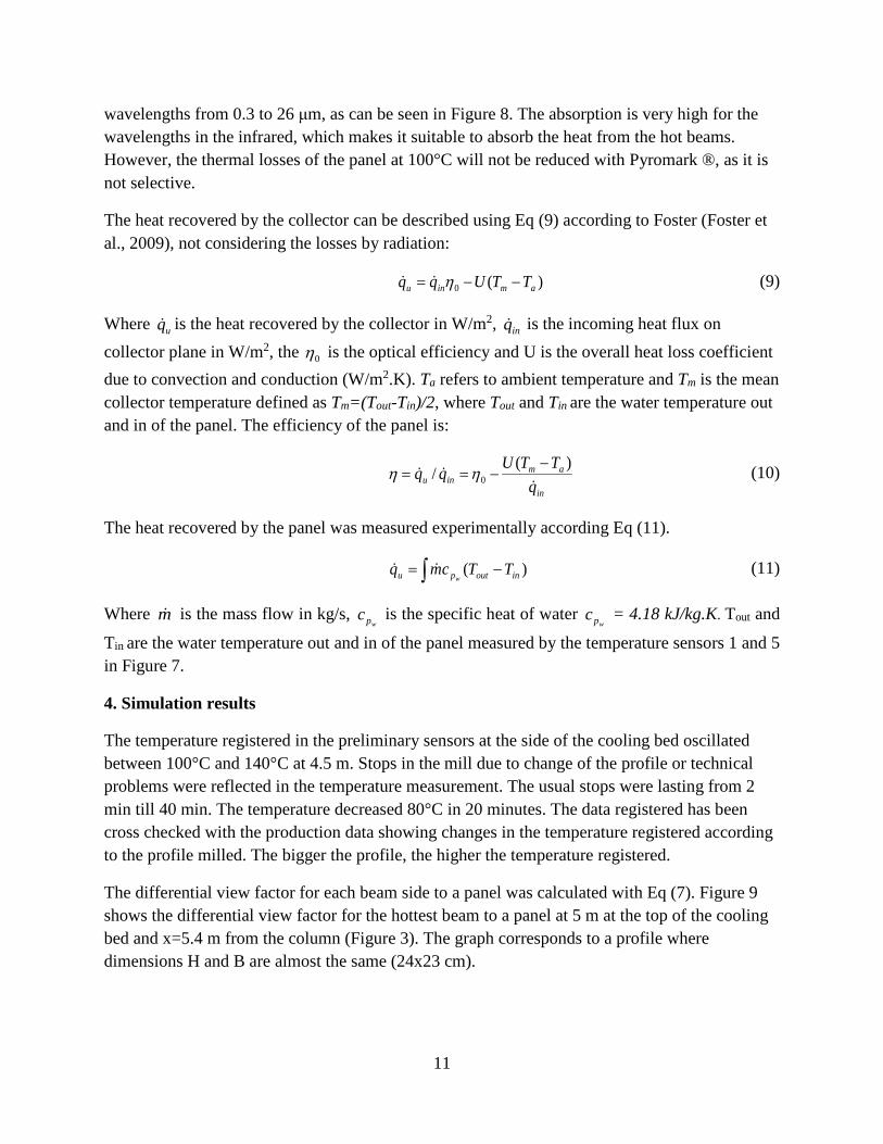
The differential view factor for each beam side to a panel was calculated with Eq (7). Figure 9 shows the differential view factor for the hottest beam to a panel at 5 m at the top of the cooling bed and x=5.4 m from the column (Figure 3). The graph corresponds to a profile where dimensions H and B are almost the same (24x23 cm).

11

Figure 9: Differential view factors 12ϕ for the first beam horizontal and vertical sides to a panel in the top of the cooling bed

The differential view factor of two thirds of the beam is negligible. Only the central 30 m of the beam transfer heat with the simulated panel. The differential view factors from the horizontal side of the beam are nine times higher than the ones for the vertical side. The horizontal side of the beam is a parallel plane from the panel, and the vertical side has a polar angle close to β1= 82°. In the case of panels situated parallel to the cooling bed (Figure 10) the influence of the vertical sideis four times bigger than the horizontal side. The vertical side has a polar angle of β1= 13°, and the horizontal side has a polar angle of β1= 78°. Figure 10 shows the differential view factors of the first beam to a panel situated at x=0 and at a height from the floor of 2.5 m and α=0° are presented (Figure 2). The more the height of the panel increases ; the more similar the influence of the two beam side as the polar angles β1 and β2 get closer. However the maximum differential view factor is lower.

12

Figure 10: Differential view factors for the first beam horizontal and vertical sides to a panel in the side of the cooling bed

The heat flux received by the panels at the side of the cooling bed was simulated for different heights and inclinations. Treating all the data for all the profiles, the maximum heat flux received by the panel from the biggest and the smallest beam is achieved at 3.5 m and 4.5 m at α=20° and α=30°. Figure 11 shows the panel inclination for each height with the maximum heat flux received by the panel. According to these results the simulated heat flux is very similar for the four different heights simulated. The profiles are organized by decreasing beam perimeter. However beams with the same perimeter can have different height and width dimensions resulting in a different heat flux arriving to the panel what explains the existence of the peaks in the curves.

Figure 11: Simulated heat flux for the most favourable heights and inclinations

00.5

11.5

22.5

33.5

44.5

1.92

1.71

1.64

1.53

1.51

1.49

1.38

1.29

1.27

1.21

1.17

1.07

1.00

0.93

0.90

0.80

0.70

Hea

t flu

x [k

W/m

2]

Beam perimeter [m]

2.5m 3.5m 4.5m 5.5mα=10° α=20° α=30° α=30°

13

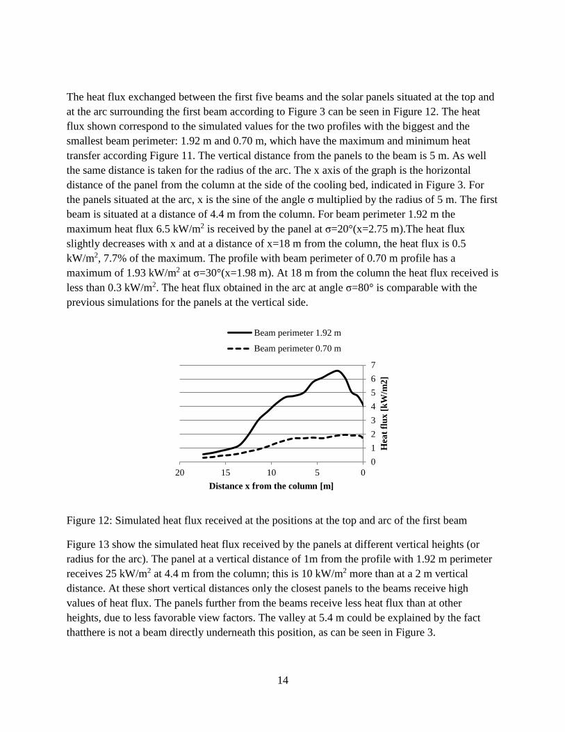
The heat flux exchanged between the first five beams and the solar panels situated at the top and at the arc surrounding the first beam according to Figure 3 can be seen in Figure 12. The heat flux shown correspond to the simulated values for the two profiles with the biggest and the smallest beam perimeter: 1.92 m and 0.70 m, which have the maximum and minimum heat transfer according Figure 11. The vertical distance from the panels to the beam is 5 m. As well the same distance is taken for the radius of the arc. The x axis of the graph is the horizontal distance of the panel from the column at the side of the cooling bed, indicated in Figure 3. For the panels situated at the arc, x is the sine of the angle σ multiplied by the radius of 5 m. The first beam is situated at a distance of 4.4 m from the column. For beam perimeter 1.92 m the maximum heat flux 6.5 kW/m2 is received by the panel at σ=20°(x=2.75 m).The heat flux slightly decreases with x and at a distance of x=18 m from the column, the heat flux is 0.5 kW/m2, 7.7% of the maximum. The profile with beam perimeter of 0.70 m profile has a maximum of 1.93 kW/m2 at σ=30°(x=1.98 m). At 18 m from the column the heat flux received is less than 0.3 kW/m2. The heat flux obtained in the arc at angle σ=80° is comparable with the previous simulations for the panels at the vertical side.

Figure 12: Simulated heat flux received at the positions at the top and arc of the first beam

Figure 13 show the simulated heat flux received by the panels at different vertical heights (or radius for the arc). The panel at a vertical distance of 1m from the profile with 1.92 m perimeter receives 25 kW/m2 at 4.4 m from the column; this is 10 kW/m2 more than at a 2 m vertical distance. At these short vertical distances only the closest panels to the beams receive high values of heat flux. The panels further from the beams receive less heat flux than at other heights, due to less favorable view factors. The valley at 5.4 m could be explained by the fact thatthere is not a beam directly underneath this position, as can be seen in Figure 3.

01234567

05101520

Hea

t flu

x [k

W/m

2]

Distance x from the column [m]

Beam perimeter 1.92 m

Beam perimeter 0.70 m

14

Figure 13: Simulated heat flux received at the positions at the top and arc for 5 vertical distances (Beam perimeter 1.92m)

As a conclusion, the simulated heat flux arriving to the panels at the side of the cooling bed (Fig. 11) is similar for all the different heights tested. The panels at height of 3.5m and 4.5m receive slightly more heat flux. The simulated heat flux received by the panels at the top of the cooling bed is higher than the heat flux received by the panels at the side of the cooling bed. At 5 m the heat flux is only 1.5 times more. However, for shorter distances is up to seven times higher, 25 kW/m2 for the bigger profiles and 7 kW/m2 for the smaller profiles. The maximum values are achieved at the panel at 4.4 m from the column at the top of the cooling bed as well as in the higher positions of the arc.

5. Experimental results

The different absorbers were tested for several heights and inclinations. Different flows and temperatures of the water flowing into the panel were analyzed. The objective was to find the optimum conditions for recovering the maximum amount of energy at the highest temperature level. The measurement period studied was 131 days. During this period there were 18 days were a non painted panel has been tested and the rest of the 113 days with Pyromark ® painted panels.

Table 3 presents a summary of the heat and temperature values for the different panels (according Fig. 2). The average is the pondered average of all the profiles produced during each test period.

Panel h α Time Energy recovered

Energy recovered

per ton

Average Heat

recovered

Max. Heat

recovered

Average Temp.

Out

Maximum Temp.

Out

Average Heat

received

Efficiency

m ° H kWh/m2 kWh/t.m2 kW/m2 kW/m2 °C °C kW/m2

HP 4.5 0 339 142 0.0039 0.42 0.88 52 70 n.a. n.a.

0

5

10

15

20

25

30

05101520

kW/m

2

Distance x from the column [m]

5m 4m 3m 2m 1m

15

DM 3.5 0 350 305 0.0073 0.86 1.53 73 95 n.a. n.a.

DM 4.5 0 279 249 0.0072 0.87 1.53 75 101 n.a. n.a.

DM 5.0 0 90 64 0.0079 0.69 1.36 70 93 n.a. n.a.

DM 3.5 0 169 157 0.0066 0.96 1.49 74 95 2.3 0.42

TOTAL DM 888 775 0.0072 0.87 1.53 74 101 n.a. n.a.

BC 4.5 0 110 111 0.0083 0.96 1.50 67 95 1.9 0.51

BC 2.5 0 330 206 0.0077 0.61 1.31 51 84 1.66 0.37

BC 3.5 20 280 225 0.0063 0.79 1.50 57 84 2.08 0.38

BC 3.5 0 190 124 0.0053 0.63 1.01 77 104 1.98 0.32

BC 4.5 20 345 233 0.0057 0.67 1.08 80 119 1.90 0.35

BC 4.5 0 201 142 0.0035 0.7 1.05 81 117 2 0.35

TOTAL BC 1456 1041 0.0067 0.73 1.50 69 119 1.95 0.36

TOTAL PAINTED 2344 1816 0.0060 0.77 1.53 70 119 1.97 0.39

n.a.=not available HP:Full sheet harp absorber (Not painted)

DM: Full sheet absorber with double meander (Painted with Pyromark ®) BC: Harp absorber with fins black chrome coated (Painted with Pyromark ®)

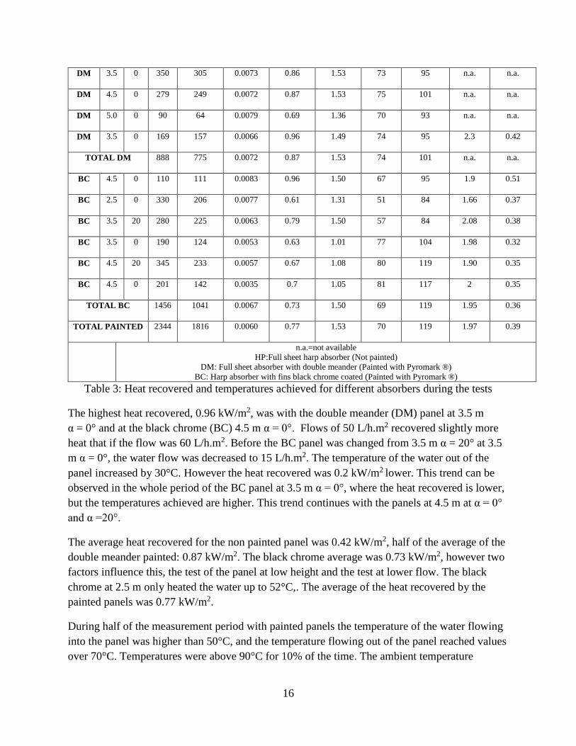
Table 3: Heat recovered and temperatures achieved for different absorbers during the tests

The highest heat recovered, 0.96 kW/m2, was with the double meander (DM) panel at 3.5 m α = 0° and at the black chrome (BC) 4.5 m α = 0°. Flows of 50 L/h.m2 recovered slightly more heat that if the flow was 60 L/h.m2. Before the BC panel was changed from 3.5 m α = 20° at 3.5 m α = 0°, the water flow was decreased to 15 L/h.m2. The temperature of the water out of the panel increased by 30°C. However the heat recovered was 0.2 kW/m2 lower. This trend can be observed in the whole period of the BC panel at 3.5 m α = 0°, where the heat recovered is lower, but the temperatures achieved are higher. This trend continues with the panels at 4.5 m at α = 0° and α =20°.

The average heat recovered for the non painted panel was 0.42 kW/m2, half of the average of the double meander painted: 0.87 kW/m2. The black chrome average was 0.73 kW/m2, however two factors influence this, the test of the panel at low height and the test at lower flow. The black chrome at 2.5 m only heated the water up to 52°C,. The average of the heat recovered by the painted panels was 0.77 kW/m2.

During half of the measurement period with painted panels the temperature of the water flowing into the panel was higher than 50°C, and the temperature flowing out of the panel reached values over 70°C. Temperatures were above 90°C for 10% of the time. The ambient temperature

16

registered was over 60°C during half of the period of measurements. The temperatures on the panel reached 90°C during half of the time.

More than 0.8 kW/m2 was recovered during half time of the test period with painted panels. The incident heat flux measured values were 2 kW/m2 with peaks of 4 kW/m2. The heat recovered values are slightly lower than the 1.03 kW/m2 recovered in Nilsson (Nilsson, 2003). If the tests are compared in terms of energy recovered per tonne of steel, the difference is of 6 times, 0.05 kWh/(t.m2) and 0.008 kWh/(t.m2), Swedish and Luxembourgish results respectively. This means that with less tonnage the Swedish test recovered more heat.

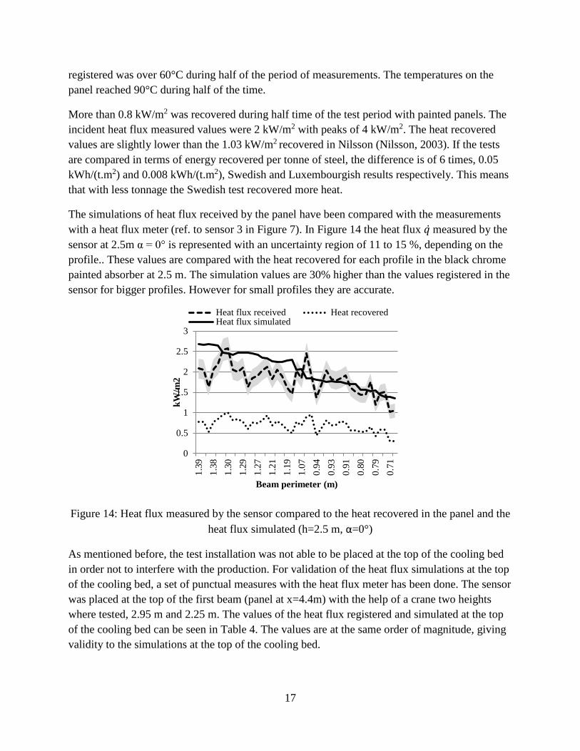
The simulations of heat flux received by the panel have been compared with the measurements with a heat flux meter (ref. to sensor 3 in Figure 7). In Figure 14 the heat flux 𝑞𝑞 ̇ measured by the sensor at 2.5m α = 0° is represented with an uncertainty region of 11 to 15 %, depending on the profile.. These values are compared with the heat recovered for each profile in the black chrome painted absorber at 2.5 m. The simulation values are 30% higher than the values registered in the sensor for bigger profiles. However for small profiles they are accurate.

Figure 14: Heat flux measured by the sensor compared to the heat recovered in the panel and the heat flux simulated (h=2.5 m, α=0°)

As mentioned before, the test installation was not able to be placed at the top of the cooling bed in order not to interfere with the production. For validation of the heat flux simulations at the top of the cooling bed, a set of punctual measures with the heat flux meter has been done. The sensor was placed at the top of the first beam (panel at x=4.4m) with the help of a crane two heights where tested, 2.95 m and 2.25 m. The values of the heat flux registered and simulated at the top of the cooling bed can be seen in Table 4. The values are at the same order of magnitude, giving validity to the simulations at the top of the cooling bed.

0

0.5

1

1.5

2

2.5

3

1.39

1.38

1.30

1.29

1.27

1.21

1.19

1.07

0.94

0.93

0.91

0.80

0.79

0.71

kW/m

2

Beam perimeter (m)

Heat flux received Heat recoveredHeat flux simulated

17

Location Heat flux measured Heat flux simulated

kW/m2 kW/m2

Y=4.5 m

X=0 m

3 2.36

Y=2.95

X=4.75

4.25 4.36

Y=2.25

X=4.75

5.95 5.63

Table 4: Heat flux measures at the top of the cooling bed compared to the simulated values

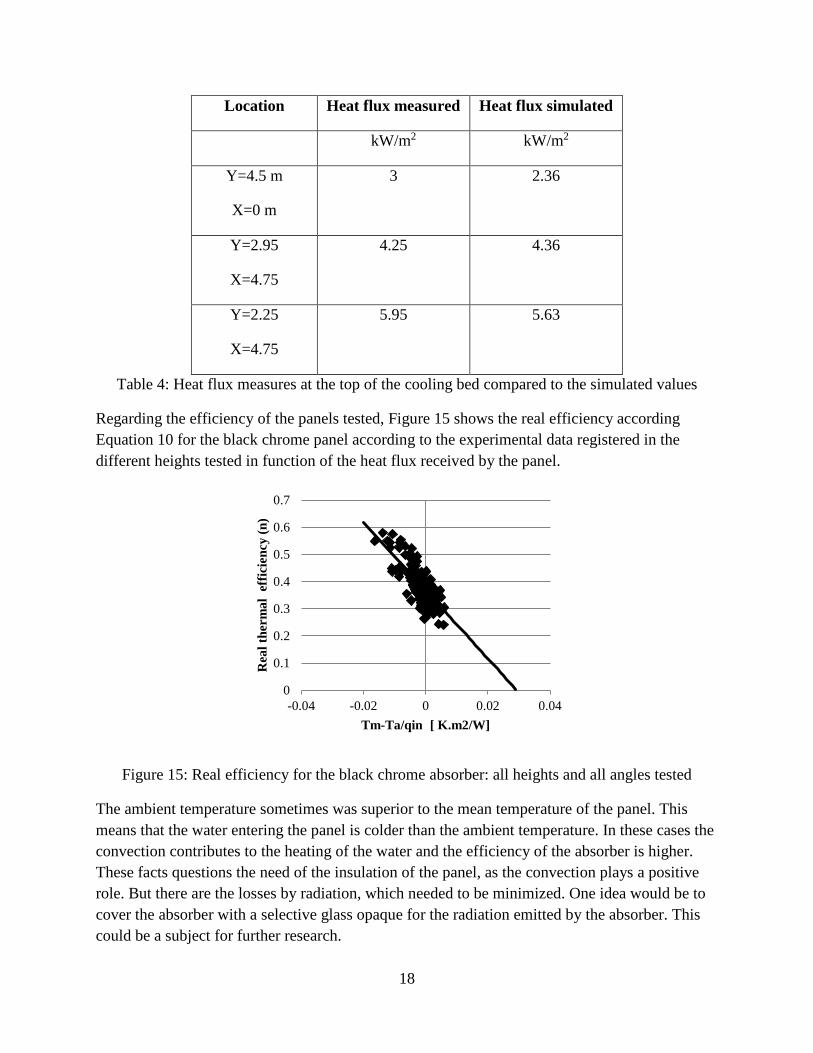
Regarding the efficiency of the panels tested, Figure 15 shows the real efficiency according Equation 10 for the black chrome panel according to the experimental data registered in the different heights tested in function of the heat flux received by the panel.

Figure 15: Real efficiency for the black chrome absorber: all heights and all angles tested

The ambient temperature sometimes was superior to the mean temperature of the panel. This means that the water entering the panel is colder than the ambient temperature. In these cases the convection contributes to the heating of the water and the efficiency of the absorber is higher. These facts questions the need of the insulation of the panel, as the convection plays a positive role. But there are the losses by radiation, which needed to be minimized. One idea would be to cover the absorber with a selective glass opaque for the radiation emitted by the absorber. This could be a subject for further research.

0

0.1

0.2

0.3

0.4

0.5

0.6

0.7

-0.04 -0.02 0 0.02 0.04

Rea

l the

rmal

eff

icie

ncy

(n)

Tm-Ta/qin [ K.m2/W]

18

The trendline obtained in Figure 15 can be expressed:

in

am

q

TTmW

)(56.12368.0

2 −−=η (12)

Hence the collector has an optical efficiency (η0) of 0.368≈37% which is rather low and an U value of 12.6 W/m2.K, which is very high. These values clearly indicate that the collector is not well designed for the targeted heat source compared to the standard solar collectors as can be seen in Figure 16.

Figure 16: Efficiency of the absorber tested compared to efficiencies of typical solar collectors (Nielsen, 2006)

The potential heat recovered at different panel locations has been calculated combining simulated heat flux values and the efficiency curve obtained in the experimental tests (Eq (12). Different flow configurations and temperatures were simulated by iteration. The panels were considered to have a surface of 1m2. Two panel location scenarios have been considered: panels at the side of the cooling bed and panels at the top of the cooling bed at a vertical distance of 3 m.

The panels at the side of the cooling bed were assumed to be situated from 15 m to 85 m parallel to the cooling bed. The panels would be placed up to 4 meters high, from 2.5 m to 6.5 m as can be seen in Figure 2. Figure 9 and 10 shows that the maximum heat transfer between the beam and the panel is between the center point of the panel and 15 m of beam in both sides. Therefore the first panel was assumed to be placed at 15 m from the beginning of the cooling bed and the last panel at 15 m from the end of the cooling bed. A total of 280 m2 of panels working in parallel were considered for the iterative calculations.

0.00

0.20

0.40

0.60

0.80

1.00

0 0.05 0.1 0.15

Effic

ienc

y [-

]

Tm-Ta/qin [K.m2/W]

Evacuated tube Flat plateUn-glazed Collector tested

19

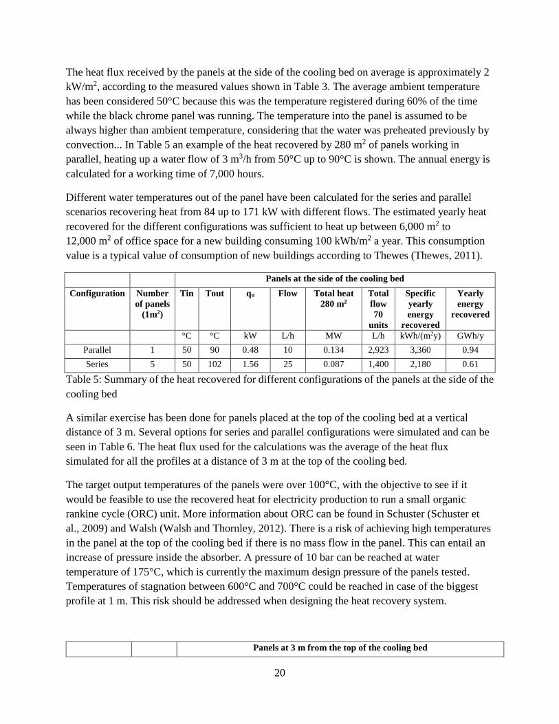
The heat flux received by the panels at the side of the cooling bed on average is approximately 2 kW/m2, according to the measured values shown in Table 3. The average ambient temperature has been considered 50°C because this was the temperature registered during 60% of the time while the black chrome panel was running. The temperature into the panel is assumed to be always higher than ambient temperature, considering that the water was preheated previously by convection... In Table 5 an example of the heat recovered by 280 m2 of panels working in parallel, heating up a water flow of 3 m3/h from 50°C up to 90°C is shown. The annual energy is calculated for a working time of 7,000 hours.

Different water temperatures out of the panel have been calculated for the series and parallel scenarios recovering heat from 84 up to 171 kW with different flows. The estimated yearly heat recovered for the different configurations was sufficient to heat up between 6,000 m2 to 12,000 m2 of office space for a new building consuming 100 kWh/m2 a year. This consumption value is a typical value of consumption of new buildings according to Thewes (Thewes, 2011).

Panels at the side of the cooling bed Configuration Number

of panels (1m2)

Tin Tout qu Flow Total heat 280 m2

Total flow 70

units

Specific yearly energy

recovered

Yearly energy

recovered

°C °C kW L/h MW L/h kWh/(m2y) GWh/y Parallel 1 50 90 0.48 10 0.134 2,923 3,360 0.94 Series 5 50 102 1.56 25 0.087 1,400 2,180 0.61

Table 5: Summary of the heat recovered for different configurations of the panels at the side of the cooling bed

A similar exercise has been done for panels placed at the top of the cooling bed at a vertical distance of 3 m. Several options for series and parallel configurations were simulated and can be seen in Table 6. The heat flux used for the calculations was the average of the heat flux simulated for all the profiles at a distance of 3 m at the top of the cooling bed.

The target output temperatures of the panels were over 100°C, with the objective to see if it would be feasible to use the recovered heat for electricity production to run a small organic rankine cycle (ORC) unit. More information about ORC can be found in Schuster (Schuster et al., 2009) and Walsh (Walsh and Thornley, 2012). There is a risk of achieving high temperatures in the panel at the top of the cooling bed if there is no mass flow in the panel. This can entail an increase of pressure inside the absorber. A pressure of 10 bar can be reached at water temperature of 175°C, which is currently the maximum design pressure of the panels tested. Temperatures of stagnation between 600°C and 700°C could be reached in case of the biggest profile at 1 m. This risk should be addressed when designing the heat recovery system.

Panels at 3 m from the top of the cooling bed

20

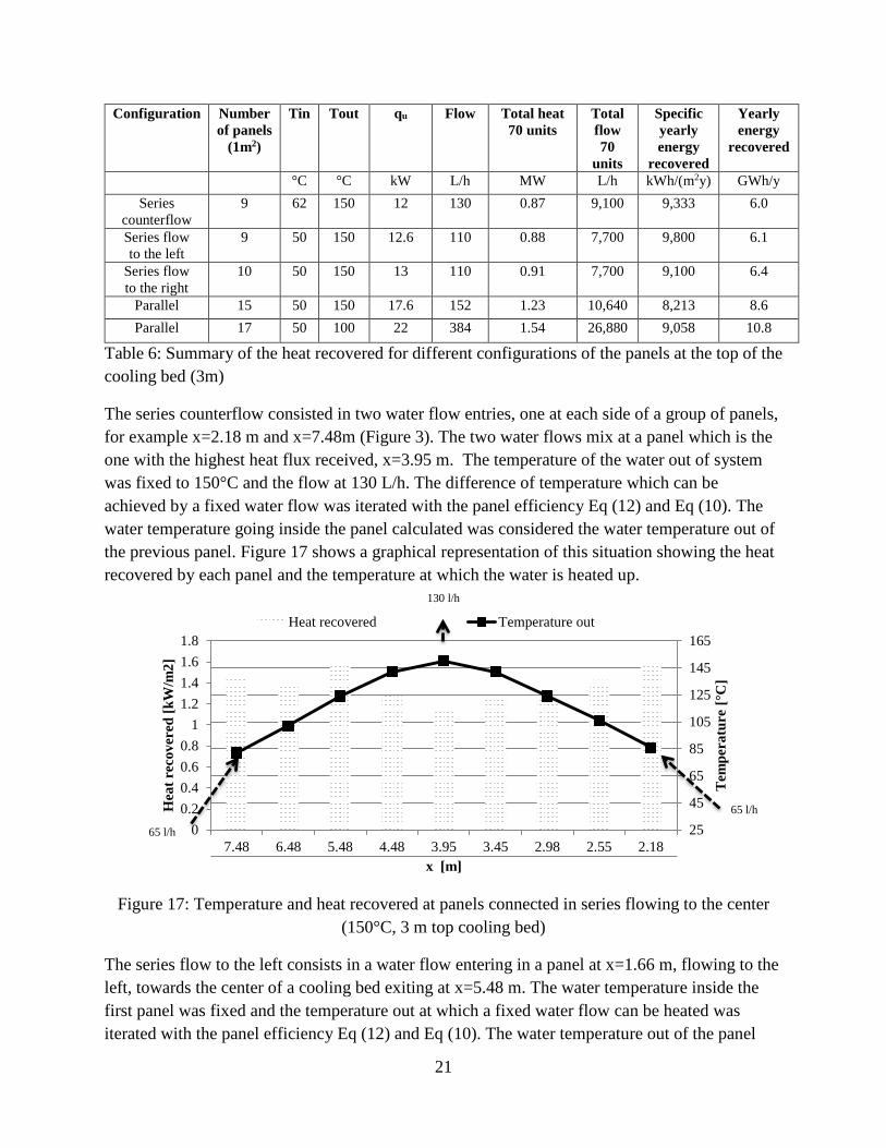
Configuration Number of panels

(1m2)

Tin Tout qu Flow Total heat 70 units

Total flow 70

units

Specific yearly energy

recovered

Yearly energy

recovered

°C °C kW L/h MW L/h kWh/(m2y) GWh/y Series

counterflow 9 62 150 12 130 0.87 9,100 9,333 6.0

Series flow to the left

9 50 150 12.6 110 0.88 7,700 9,800 6.1

Series flow to the right

10 50 150 13 110 0.91 7,700 9,100 6.4

Parallel 15 50 150 17.6 152 1.23 10,640 8,213 8.6 Parallel 17 50 100 22 384 1.54 26,880 9,058 10.8

Table 6: Summary of the heat recovered for different configurations of the panels at the top of the cooling bed (3m)

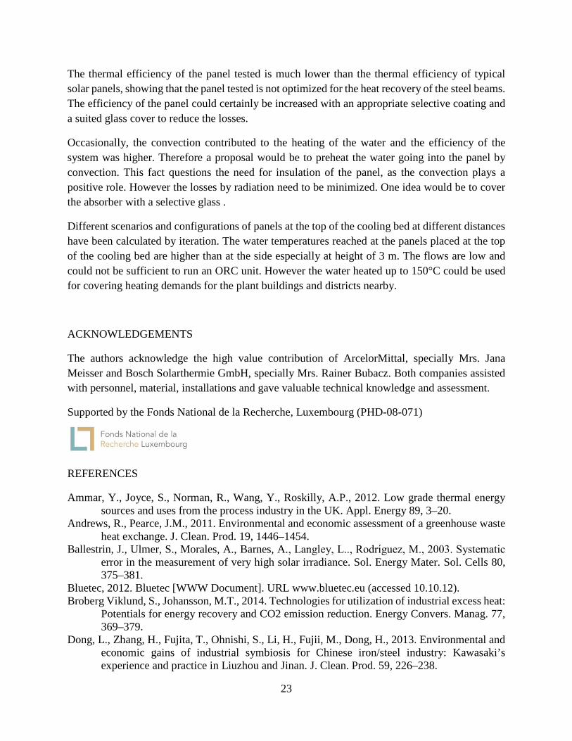
The series counterflow consisted in two water flow entries, one at each side of a group of panels, for example x=2.18 m and x=7.48m (Figure 3). The two water flows mix at a panel which is the one with the highest heat flux received, x=3.95 m. The temperature of the water out of system was fixed to 150°C and the flow at 130 L/h. The difference of temperature which can be achieved by a fixed water flow was iterated with the panel efficiency Eq (12) and Eq (10). The water temperature going inside the panel calculated was considered the water temperature out of the previous panel. Figure 17 shows a graphical representation of this situation showing the heat recovered by each panel and the temperature at which the water is heated up.

Figure 17: Temperature and heat recovered at panels connected in series flowing to the center (150°C, 3 m top cooling bed)

The series flow to the left consists in a water flow entering in a panel at x=1.66 m, flowing to the left, towards the center of a cooling bed exiting at x=5.48 m. The water temperature inside the first panel was fixed and the temperature out at which a fixed water flow can be heated was iterated with the panel efficiency Eq (12) and Eq (10). The water temperature out of the panel

00.20.40.60.8

11.21.41.61.8

25

45

65

85

105

125

145

165

2.182.552.983.453.954.485.486.487.48

Hea

t rec

over

ed [k

W/m

2]

Tem

pera

ture

[°C

]

x [m]

Heat recovered Temperature out

130 l/h

65 l/h

65 l/h

21

was considered to be the water temperature inside the next panel. The same exercise was done from panel at x=7.48 m and flowing to the right until panel at x=1.88m. At the parallel configuration, each panel heated up a certain flow of water to a fixed temperature according to the heat flux received and the efficiency of the panel.

The calculated yearly heat recovered is sufficient to heat 25,000 m2 up to 250,000 m2 of office space. In the coldest month energy of 0.6 up to 1.8 GWh could be delivered, covering the building heating needs of the steel plant studied for this month. The specific yearly energy recovered (kWh/m2/year) is significantly higher than a typical flat solar absorber in Luxembourg around 350 kWh/m2/year and of a vacuum absorber around 450 kWh/m2/year.

As a summary of this section, elevated water temperatures can be reached if panels are placed at the top of the cooling bed, especially at height of 3 m. The flows obtained are low and could not be sufficient to run an ORC unit. However the water heated up to 150°C could be used for covering heating demands for the plant buildings and the districts nearby. The panels on the side of the cooling bed, offer less heat recovery potential, heating only up to 100°C and with lower flows.

For further research, a detailed study of the interaction of the heat recovery in the panels with the cooling process of the beam is proposed. The cooling by natural convection of the cooling bed would be affected by the placement of panels on the top. These panels need to be placed at an angle to allow the air to flow between them. As well the cooling by radiation would also be affected. The heat exchange between the beam and the panel will be different than the current heat exchange of the beam with the environment.

6.Conclusions

A system to recover the radiative heat lost by the beams in the cooling bed was devised and a pilot test installed in one of the cooling beds of the plant.

Simulations of the heat flux exchanged with solar absorbers at different orientations, heights and inclinations were validated by experimental results. The simulations are accurate for small profiles. The heat flux received by the panels next to the cooling bed is similar for the different heights. However, the heat flux received by the panels at short distance at the top of the cooling bed are up to seven times higher than at the side.

A test installation with standard solar absorbers slightly modified, was placed at the side of the cooling bed and the average heat recovered was 0.77 kW/m2, during the whole period where the absorbers were painted with Pyromark ®. For certain water flows and heights, averages of 0.96 kW/m2 were achieved. This value is similar to the heat recovered in the rolling mill example in Nilsson (Nilsson, 2003). Regarding temperatures, half of the time the temperatures were above 70°C, and 10% of the time at 90°C.

22

The thermal efficiency of the panel tested is much lower than the thermal efficiency of typical solar panels, showing that the panel tested is not optimized for the heat recovery of the steel beams. The efficiency of the panel could certainly be increased with an appropriate selective coating and a suited glass cover to reduce the losses.

Occasionally, the convection contributed to the heating of the water and the efficiency of the system was higher. Therefore a proposal would be to preheat the water going into the panel by convection. This fact questions the need for insulation of the panel, as the convection plays a positive role. However the losses by radiation need to be minimized. One idea would be to cover the absorber with a selective glass .

Different scenarios and configurations of panels at the top of the cooling bed at different distances have been calculated by iteration. The water temperatures reached at the panels placed at the top of the cooling bed are higher than at the side especially at height of 3 m. The flows are low and could not be sufficient to run an ORC unit. However the water heated up to 150°C could be used for covering heating demands for the plant buildings and districts nearby.

ACKNOWLEDGEMENTS

The authors acknowledge the high value contribution of ArcelorMittal, specially Mrs. Jana Meisser and Bosch Solarthermie GmbH, specially Mrs. Rainer Bubacz. Both companies assisted with personnel, material, installations and gave valuable technical knowledge and assessment.

Supported by the Fonds National de la Recherche, Luxembourg (PHD-08-071)

REFERENCES

Ammar, Y., Joyce, S., Norman, R., Wang, Y., Roskilly, A.P., 2012. Low grade thermal energy sources and uses from the process industry in the UK. Appl. Energy 89, 3–20.

Andrews, R., Pearce, J.M., 2011. Environmental and economic assessment of a greenhouse waste heat exchange. J. Clean. Prod. 19, 1446–1454.

Ballestrin, J., Ulmer, S., Morales, A., Barnes, A., Langley, L.., Rodrı́guez, M., 2003. Systematic error in the measurement of very high solar irradiance. Sol. Energy Mater. Sol. Cells 80, 375–381.

Bluetec, 2012. Bluetec [WWW Document]. URL www.bluetec.eu (accessed 10.10.12). Broberg Viklund, S., Johansson, M.T., 2014. Technologies for utilization of industrial excess heat:

Potentials for energy recovery and CO2 emission reduction. Energy Convers. Manag. 77, 369–379.

Dong, L., Zhang, H., Fujita, T., Ohnishi, S., Li, H., Fujii, M., Dong, H., 2013. Environmental and economic gains of industrial symbiosis for Chinese iron/steel industry: Kawasaki’s experience and practice in Liuzhou and Jinan. J. Clean. Prod. 59, 226–238.

23

Eurostat, E.C., 2009. Energy, transport and environment indicators. Office for official publications of the European communities, Luxembourg, Luxembourg.

Foster, R., Ghassemi, M., Cota, A., 2009. Solar Energy: Renewable Energy and the Environment, 1st ed. CRC Press, Boca Raton, Fla. USA.

Johansson, M.T., Söderström, M., 2011. Options for the Swedish steel industry – Energy efficiency measures and fuel conversion. Energy 36, 191–198.

Kabelac, S., Vortmeyer, D., 2010. K1 Radiation of Surfaces, in: VDI Heat Atlas, VDI-Buch. Springer Berlin Heidelberg, Germany, pp. 945–960.

Kennedy, C.E., 2002. Review of mid-to-high-temperature solar selective absorber materials. National Renewable Energy Laboratory. U.S.Department of Energy, Oak Ridge, TN, USA.

Kirschen, M., Risonarta, V., Pfeifer, H., 2009. Energy efficiency and the influence of gas burners to the energy related carbon dioxide emissions of electric arc furnaces in steel industry. Energy 34, 1065–1072.

Ma, G., Cai, J., Zeng, W., Dong, H., 2012. Analytical Research on Waste Heat Recovery and Utilization of China’s Iron & Steel Industry. Energy Procedia 14, 1022–1028.

Mahan, J.R., 2002. Radiation Heat Transfer: A Statistical Approach. John Wiley & Sons. Moya, J.A., Pardo, N., 2013. The potential for improvements in energy efficiency and CO2

emissions in the EU27 iron and steel industry under different payback periods. J. Clean. Prod. 52, 71–83.

Nielsen, J.E., 2006. Efficiency program_SK_test. ESTIF. Available at: www.estif.org/solarkeymarknew/.

Nilsson, J., 2003. Heat recovery from cooling beds in the iron & steel industry. 100 times better than solar [Värmeåtervinning från svalbäddar inom järnoch stålindustrin: Värme från svalbäddar e 100 gånger bättre än solvärme] ( No. 809). Jerkontorets Forskning [in Swedish], Sweden.

Schuster, A., Karellas, S., Kakaras, E., Spliethoff, H., 2009. Energetic and economic investigation of Organic Rankine Cycle applications. Appl. Therm. Eng. 29, 1809–1817.

Tarres Font, J., Maas, S., Scholzen, F., Zürbes, A., Meisser, J., 2011. Integrative analysis of the energy flow in a steel plant and a comprehensive approach to increase the energy efficiency, in: Proceedings METEC InSteelCON 2011. Presented at the 1st International Conference on Energy Efficiency and CO2 Reduction in the Steel Industry, Düsseldorf, p. Session 14. Pages 1–10.

Tempil, 2012. Tempil [WWW Document]. URL www.tempil.com/products/pyromark/ (accessed 1.2.12).

Thewes, A., 2011. Energieeffizienz neuer Schul- und Bürogebäude in Luxemburg basierend auf Verbrauchsdaten und Simulationen, 1., Aufl. ed. Shaker, Germany.

Walsh, C., Thornley, P., 2012. The environmental impact and economic feasibility of introducing an Organic Rankine Cycle to recover low grade heat during the production of metallurgical coke. J. Clean. Prod. 34, 29–37.

Zavoico, A.B., 2001. Solar Power Tower. Design Basis Document. Sandia National Laboratories. United States Department of Energy, Albuquerque, New Mexico, USA.

24