Experimental investigation of heat recovery from R744 ...418902/FULLTEXT01.pdf · Experimental investigation of heat ... Experimental investigation of heat recovery from R744 based

Experimental investigation of heat recovery from R744 based

refrigeration system

ZAHID ANWAR

Master of Science Thesis

KTH School of Industrial Engineering and Management

Energy Technology EGI-2011-02MSC

Division of Applied thermodynamics & Refrigeration

SE-100 44 STOCKHOLM

iii

Experimental investigation of heat recovery

from R744 based refrigeration system

Zahid Anwar

Master of Science Thesis Energy Technology 2011:02MSC

KTH School of Industrial Engineering and Management

Division of Applied Thermodynamic and Refrigeration

SE-100 44 STOCKHOLM

iv

v

Master of Science Thesis EGI 2011/ETT:02MSC

Experimental investigation of heat recovery from

R744 based refrigeration system

Zahid Anwar

Approved

Date

Examiner

Professor Per Lundqvist

Supervisor

Yang Chen

Commissioner

Contact person

Abstract

With increasing energy price and concern on environmental impacts, more attention has been

paid to refrigeration and heat pump systems. Several regulations have already been applied

on the choice of refrigerants and the search for more energy efficient system solutions has

been intensified. Due to these reasons, CO2 as an environmental benign natural refrigerant

has attracted great interest since 1990s.

Due to its low critical temperature (31.1 oC) and high critical pressure(73.8 bar), CO2

refrigeration cycle works as a transcritical cycle, which means part of the cycle is located in

supercritical region, where the temperature is independent of the pressure. Depending on the

heat sink fluid temperature profile the temperature glide of CO2 in the supercritical region

makes it possible for the CO2 refrigeration cycle to have less irreversibility in a heat recovery

process than traditional refrigeration cycles.

A new CO2 refrigeration/heat pump test rig is built at the division of Applied

Thermodynamics and Refrigeration to investigate CO2 refrigeration/heat pump systems. With

the newly built test rig following main tasks were performed in this thesis work,

Overall system performance on various imposed operating conditions.

Second law analysis of the system by exergy and entropy balance methods

Basic components testing, namely the heat exchangers and the compressor.

Uncertainty analysis.

vi

vii

Table of Contents

Table of Contents ..................................................................................................................... vii

List of Figures ........................................................................................................................... ix

Nomenclature ............................................................................................................................ xi

Chapter 1 .................................................................................................................................... 1

1.1 Heat pump basics ................................................................................................................. 1

1.1.1 Heat Pump ..................................................................................................................... 1

1.1.2 Heat pump classification ............................................................................................... 1

1.1.3 Why heat pump ............................................................................................................. 2

1.2 Heat pump water heater (HPWH) ........................................................................................ 3

Chapter 2 .................................................................................................................................... 5

CO2 and the transcritical cycle ................................................................................................... 5

2.1 Refrigerant progression history........................................................................................ 5

2.1.1 Ozone Layer Depletion ............................................................................................. 5

2.1.2 Global warming ........................................................................................................ 5

2.2 CO2 as refrigerant ............................................................................................................ 6

2.2.1 History of CO2 .......................................................................................................... 8

2.3 CO2 Transcritical cycle .................................................................................................... 9

2.4 CO2 heat pump water heater case studies ...................................................................... 11

Chapter No 3 ............................................................................................................................ 15

3.1 System performance Evaluation ........................................................................................ 15

3.1.1 Coefficient of Performance (COP) ............................................................................. 15

3.2 References for Transcritical cycle ................................................................................. 16

3.2.1 The modified Lorenz cycle ..................................................................................... 16

3.2.2 Ideal Lorentzen cycle .............................................................................................. 17

3.2.3 Real Lorentzen cycle ............................................................................................... 17

Chapter No 4 ............................................................................................................................ 19

Heat Pump testing at KTH ....................................................................................................... 19

4.1 CO2 heat pump at KTH (system layout) ........................................................................ 19

4.1.1 System modifications .............................................................................................. 20

4.2 Working principle .......................................................................................................... 20

4.2.1 Methodology ........................................................................................................... 21

4.2.2 Direct and Indirect mass flow measurement ........................................................... 21

4.3 Results ............................................................................................................................ 23

4.3.1 Overall system performance from meter reading ................................................... 23

Case A .......................................................................................................................... 23

Case B .......................................................................................................................... 26

Case C Part 1 ................................................................................................................ 28

Case C Part 2 ................................................................................................................ 30

Case D .......................................................................................................................... 32

viii

4.3.2 Results based on the compressor data ..................................................................... 34

Case A .......................................................................................................................... 34

Case B .......................................................................................................................... 35

Case C Part 1 ................................................................................................................ 36

Case C Part 2 ................................................................................................................ 36

Case D .......................................................................................................................... 37

4.3.3 Results for the components testing ......................................................................... 39

4.3.3.1 Heat exchanger effectiveness ........................................................................... 39

4.3.3.1.1 For the 1ST

heat exchanger ........................................................................ 39

4.3.3.1.2For the 3RD

heat exchanger ........................................................................ 41

4.4.4 Second law analysis of the transcritical cycle ......................................................... 44

Chapter 5 .................................................................................................................................. 49

Uncertainty Analysis ................................................................................................................ 49

5.1 Uncertainty in the measurement of heating capacity ..................................................... 49

5.1.1 Uncertainty in temperature measurement ............................................................... 49

5.1.2 Uncertainty in the mass flow measurement ............................................................ 50

5.2 Uncertainty in COP ........................................................................................................ 50

5.3 Uncertainty in the effectiveness ..................................................................................... 51

Conclusion ............................................................................................................................... 53

References ................................................................................................................................ 55

ix

List of Figures

Figure 1 Working principle of heat pump.................................................................................. 1

Figure 2 Classification of heat pump ......................................................................................... 2

Figure 3 Energy saving by using heat pump .............................................................................. 3

Figure 4 Annual heat pump sales within Europe [17] ............................................................... 4

Figure 5 Distribution based on heating capacity [17] ................................................................ 4

Figure 6 GWP and ODP for various refrigerants....................................................................... 6

Figure 7 Pressure temperature diagram for CO2 ....................................................................... 7

Figure 8 P_h and T_s diagram for R744 .................................................................................... 7

Figure 9 CO2 as refrigerant, usage history [4] .......................................................................... 9

Figure 10 P_h and T_s diagram for subcritical vapor compression cycle ................................. 9

Figure 11 P_h and T_s diagram for transcritical vapor compression cycle with R744 ........... 10

Figure 12 T_Q diagrams for water heating application ........................................................... 10

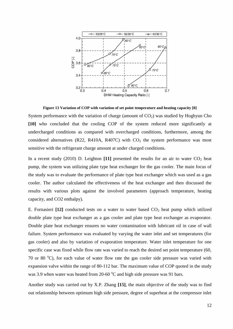
Figure 13 Variation of COP with variation of set point temperature and heating capacity [8]

.................................................................................................................................................. 12

Figure 14 Single stage CO2 heat pump cycle with decreasing gas cooler outlet temperature 16

Figure 15 T_s diagram for modified Lorentz cycle ................................................................. 16

Figure 16 T_s diagram for ideal Lorentzen cycle .................................................................... 17

Figure 17 T_s diagram for real Lorentzen cycle ...................................................................... 18

Figure 18 Schematic of CO2 heat pump at KTH ..................................................................... 19

Figure 19 CO2 heat pump after modification ........................................................................... 20

Figure 20 CO2 density variation with gas cooler outlet temperature and pressure .................. 21

Figure 21 Variation of volumetric efficiency with gas cooler pressure ................................... 23

Figure 22 COP and heating capacity with the variation of gas cooler side pressure ............... 24

Figure 23 T_h diagram for 1st Heat exchanger ....................................................................... 25

Figure 24 Lorenz efficiency (enthalpic mean temperature) with gas cooler side pressure ..... 25

Figure 25 COP and heating capacity variation with gas cooler side pressure ......................... 27

Figure 26 T_h diagram for 3rd heat exchanger ....................................................................... 28

Figure 27 Variation of Lorenz efficiency with gas cooler pressure ......................................... 28

Figure 28 Variation of COP and heating capacity with gas cooler pressure and set point

temperature .............................................................................................................................. 29


Figure 30 COP and heating capacity with gas cooler pressure ................................................ 30

Figure 31 T_h diagram (1st and 3rd heater in operation) ........................................................ 31


Figure 33 Variation of COP and heating capacity with gas cooler side pressure .................... 32

Figure 34 T_h diagram (with all three heat exchangers in operation) ..................................... 33


Figure 36 Variation of COP with approach temperature ......................................................... 34

Figure 37 Variation in COP with CO2 mass flow from compressor data ............................... 35

Figure 38 COP and variation in COP with gas cooler pressure ............................................... 35



x

Figure 41 COP and variation in COP with gas cooler side pressure ....................................... 37

Table 1 Comparative results from previous experimental studies ........................................... 38

Figure 42 Gas cooler effectiveness with approach temperature at gas cooler outlet (CO2 side)

.................................................................................................................................................. 39

Figure 43 Gas cooler effectiveness with variation in heating capacity ................................... 40

Figure 44 cooling and heating profiles with variation in approach temperature ..................... 40

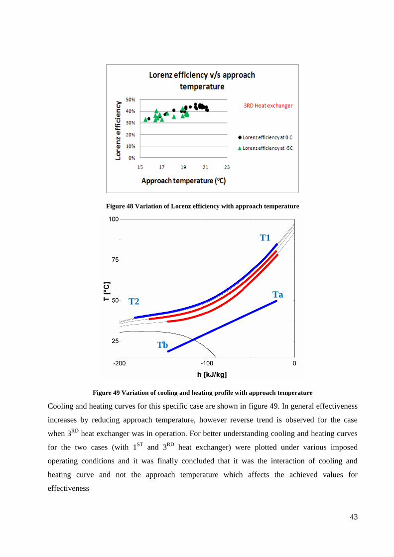
Figure 45 Lorenz efficiency with approach temperature ......................................................... 41

Figure 46 Effectiveness with approach temperature for 3RD heat exchanger ........................ 42

Figure 47 Effectiveness with heating capacity for 3RD heat exchanger ................................. 42

Figure 48 Variation of Lorenz efficiency with approach temperature .................................... 43

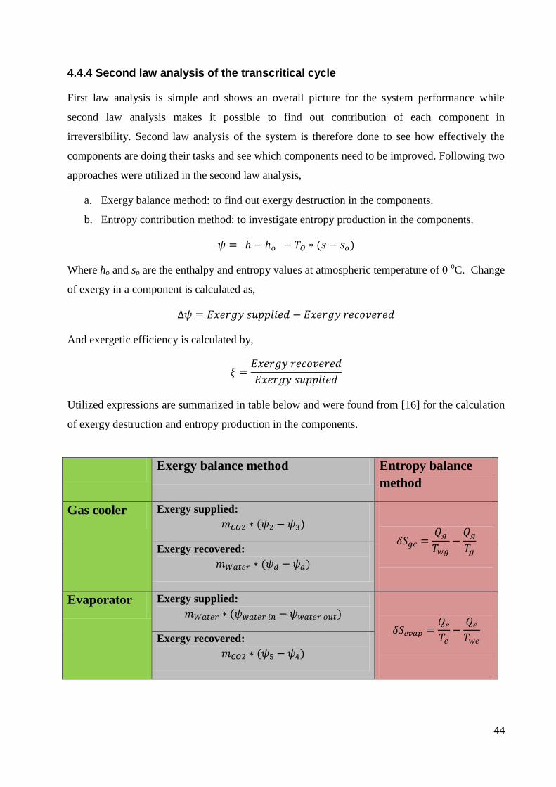
Figure 49 Variation of cooling and heating profile with approach temperature ...................... 43

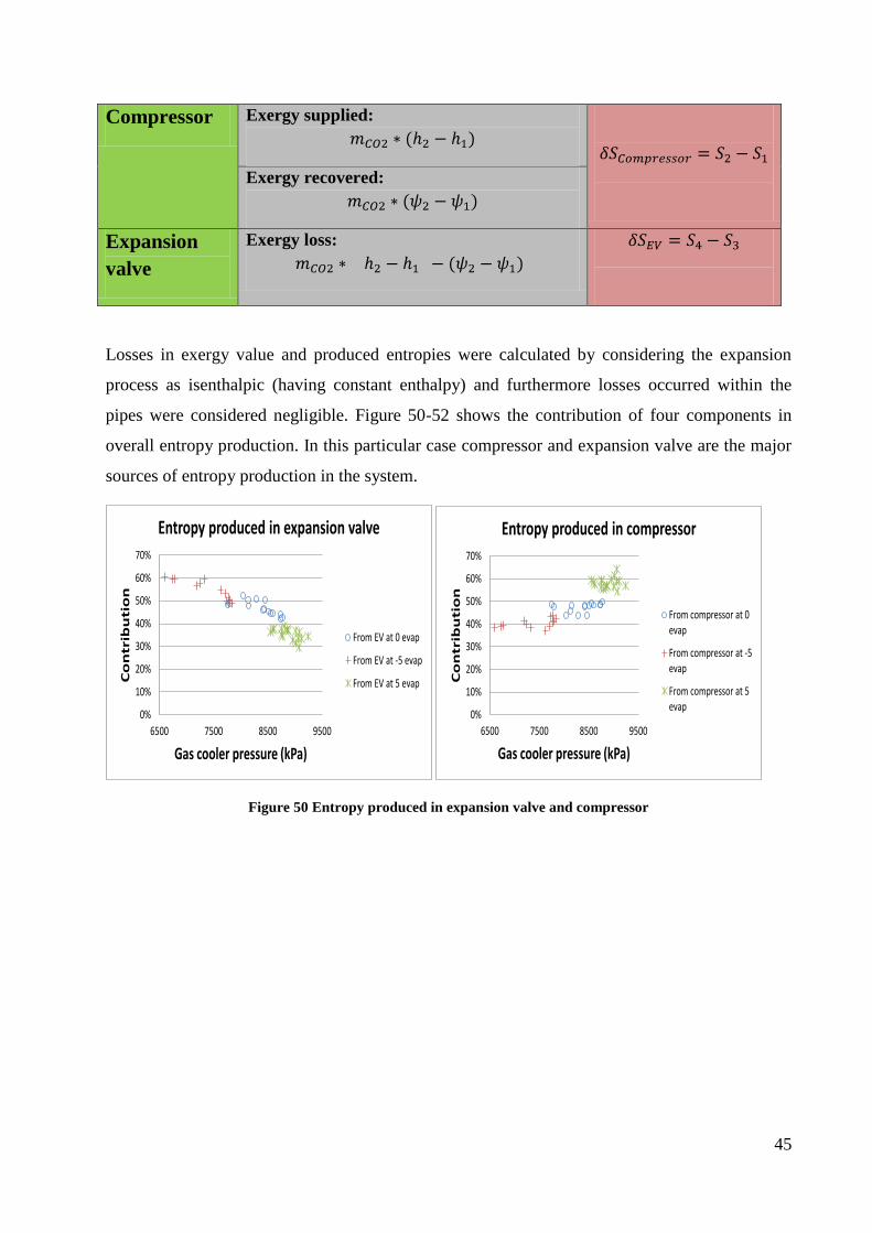
Figure 50 Entropy produced in expansion valve and compressor ........................................... 45

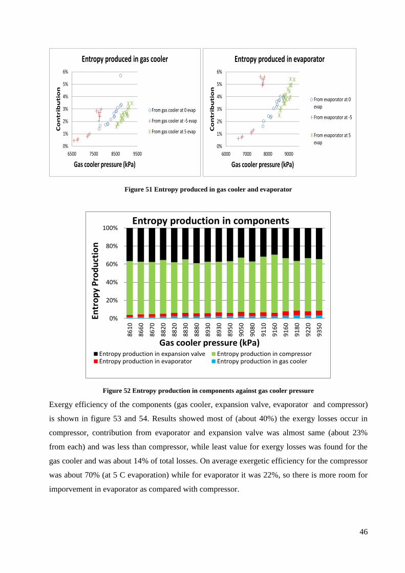
Figure 51 Entropy produced in gas cooler and evaporator ...................................................... 46

Figure 52 Entropy production in components against gas cooler pressure ............................. 46

Figure 53 Variation of exergy efficiency for compressor and expansion valve ...................... 47

Figure 54 Variation of exergy efficiency for gas cooler and evaporator ................................. 47

xi

Nomenclature

CFC Chlorofluorocarbon

HFC Hydrofluorocarbon

HCFC Hydrochloroflurocarbon

COP Coefficient of performance

HPWH Heat pump water heater

ODP Ozone depletion potential

GWP Global warming potential

TEWI Total equivalent warming impact

DHW District heating water

kW Kilowatt

Ph-diagram pressure enthalpy diagram

Ts-diagram Temperature entropy diagram

TQ-diagram Temperature heat transfer diagram

EES Engineering equation solver

RPM Revolution per minute

FS Accuracy Full scale accuracy

PR Pressure ratio

HEx Heat exchanger

Cp Specific heat

Isentropic efficiency

Volumetric efficiency

ΔT Temperature difference

Density of water

volume flow rate of water

mass flow rate of water

xii

mass flow rate of CO2

Work input to the compressor

Heat energy taken by water

Energy gain by CO2 in motor

Energy losses in the oil cooler portion

Effectiveness of the gas cooler

Swept volume flow rate of the compressor

Mean temperature (CO2) during the gas cooling process

COP based on Lorenz cycle

Lorenz efficiency

1

Chapter 1

1.1 Heat pump basics

1.1.1 Heat Pump

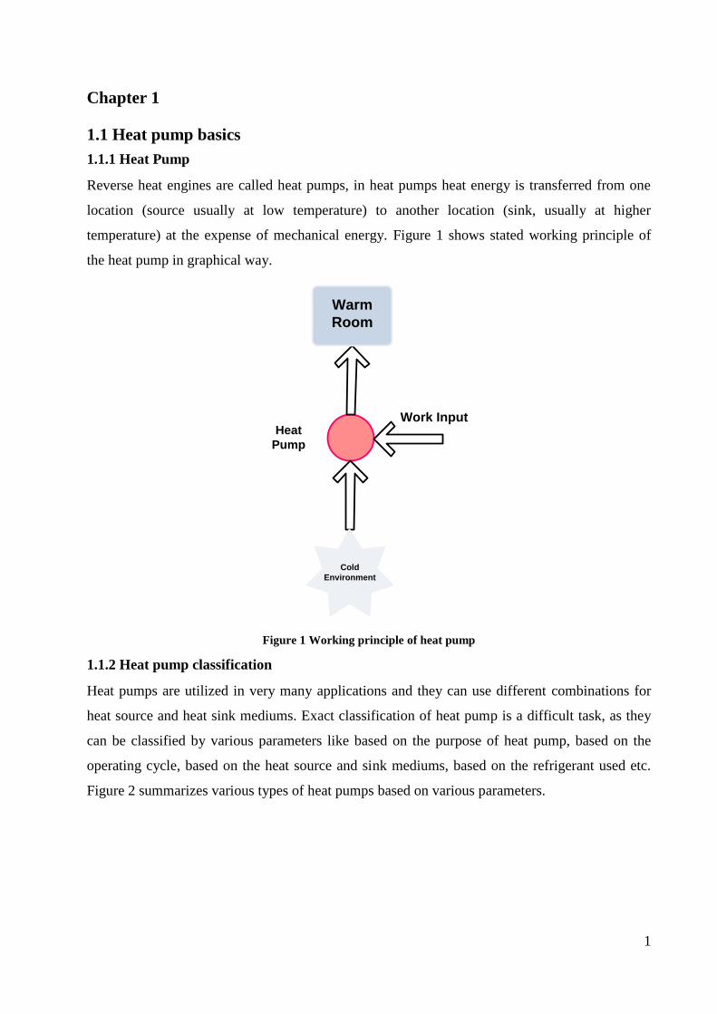
Reverse heat engines are called heat pumps, in heat pumps heat energy is transferred from one

location (source usually at low temperature) to another location (sink, usually at higher

temperature) at the expense of mechanical energy. Figure 1 shows stated working principle of

the heat pump in graphical way.

Cold

Environment

Warm

Room

Work InputHeat

Pump

Figure 1 Working principle of heat pump

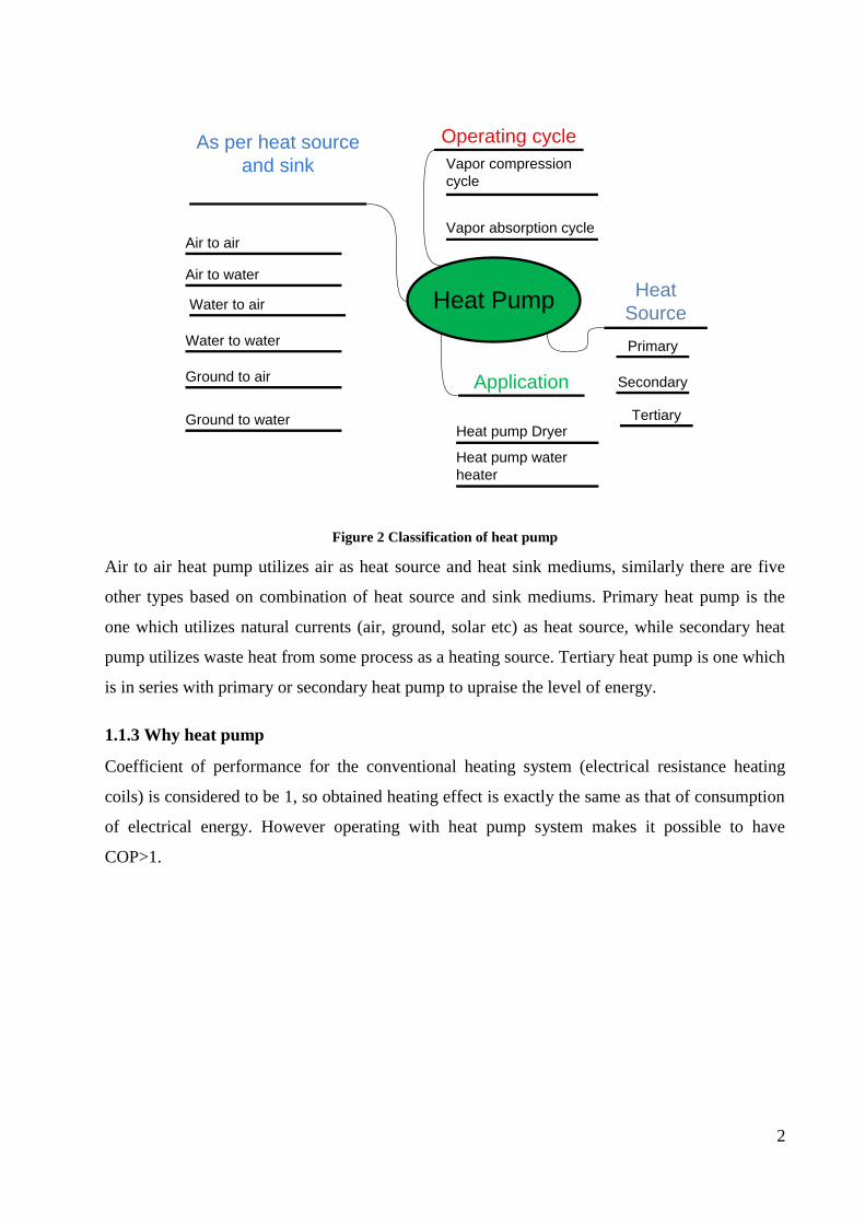
1.1.2 Heat pump classification

Heat pumps are utilized in very many applications and they can use different combinations for

heat source and heat sink mediums. Exact classification of heat pump is a difficult task, as they

can be classified by various parameters like based on the purpose of heat pump, based on the

operating cycle, based on the heat source and sink mediums, based on the refrigerant used etc.

Figure 2 summarizes various types of heat pumps based on various parameters.

2

Heat Pump

As per heat source

and sink

Air to air

Air to water

Water to air

Water to water

Ground to air

Ground to water

Operating cycle

Vapor compression

cycle

Vapor absorption cycle

Application

Heat pump Dryer

Heat pump water

heater

Heat

Source

Primary

Secondary

Tertiary

Figure 2 Classification of heat pump

Air to air heat pump utilizes air as heat source and heat sink mediums, similarly there are five

other types based on combination of heat source and sink mediums. Primary heat pump is the

one which utilizes natural currents (air, ground, solar etc) as heat source, while secondary heat

pump utilizes waste heat from some process as a heating source. Tertiary heat pump is one which

is in series with primary or secondary heat pump to upraise the level of energy.

1.1.3 Why heat pump

Coefficient of performance for the conventional heating system (electrical resistance heating

coils) is considered to be 1, so obtained heating effect is exactly the same as that of consumption

of electrical energy. However operating with heat pump system makes it possible to have

COP>1.

3

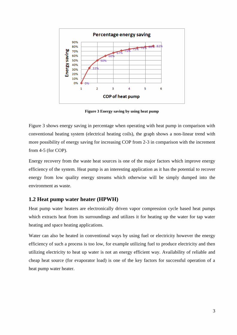
Figure 3 Energy saving by using heat pump

Figure 3 shows energy saving in percentage when operating with heat pump in comparison with

conventional heating system (electrical heating coils), the graph shows a non-linear trend with

more possibility of energy saving for increasing COP from 2-3 in comparison with the increment

from 4-5 (for COP).

Energy recovery from the waste heat sources is one of the major factors which improve energy

efficiency of the system. Heat pump is an interesting application as it has the potential to recover

energy from low quality energy streams which otherwise will be simply dumped into the

environment as waste.

1.2 Heat pump water heater (HPWH)

Heat pump water heaters are electronically driven vapor compression cycle based heat pumps

which extracts heat from its surroundings and utilizes it for heating up the water for tap water

heating and space heating applications.

Water can also be heated in conventional ways by using fuel or electricity however the energy

efficiency of such a process is too low, for example utilizing fuel to produce electricity and then

utilizing electricity to heat up water is not an energy efficient way. Availability of reliable and

cheap heat source (for evaporator load) is one of the key factors for successful operation of a

heat pump water heater.

4

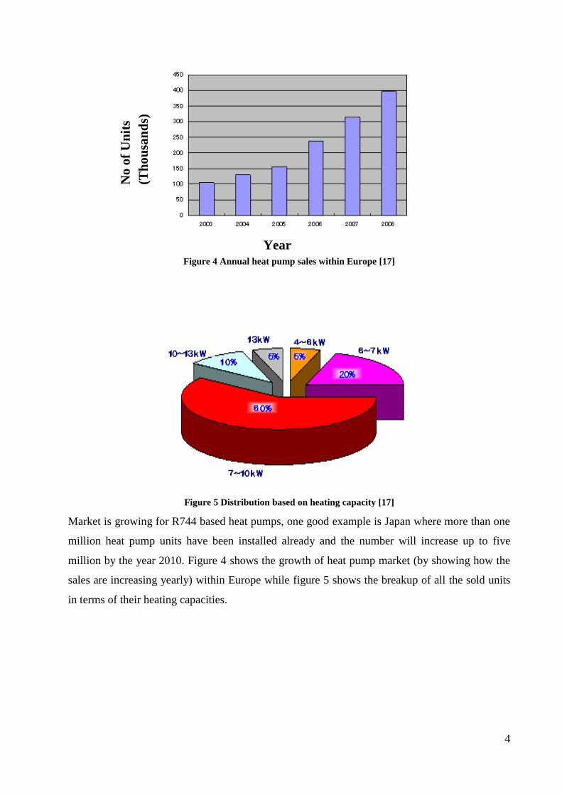
Figure 4 Annual heat pump sales within Europe [17]

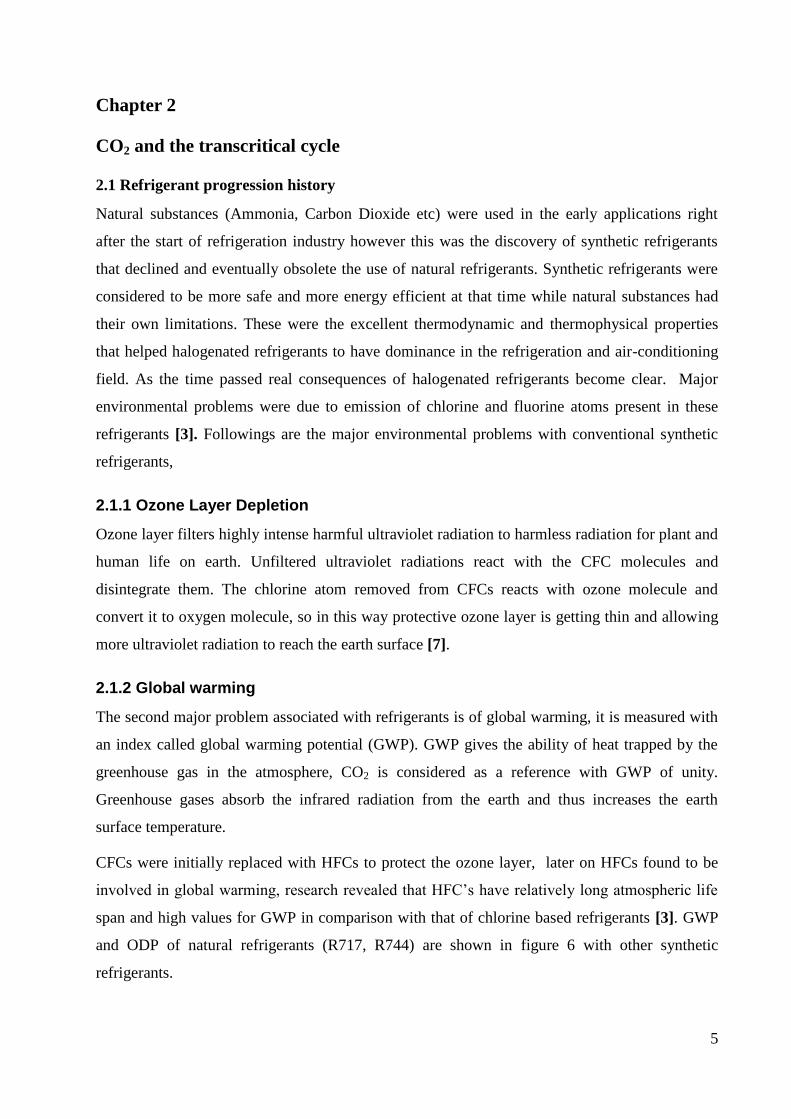
Figure 5 Distribution based on heating capacity [17]

Market is growing for R744 based heat pumps, one good example is Japan where more than one

million heat pump units have been installed already and the number will increase up to five

million by the year 2010. Figure 4 shows the growth of heat pump market (by showing how the

sales are increasing yearly) within Europe while figure 5 shows the breakup of all the sold units

in terms of their heating capacities.

No

of

Un

its

(Th

ou

san

ds)

Year

5

Chapter 2

CO2 and the transcritical cycle

2.1 Refrigerant progression history

Natural substances (Ammonia, Carbon Dioxide etc) were used in the early applications right

after the start of refrigeration industry however this was the discovery of synthetic refrigerants

that declined and eventually obsolete the use of natural refrigerants. Synthetic refrigerants were

considered to be more safe and more energy efficient at that time while natural substances had

their own limitations. These were the excellent thermodynamic and thermophysical properties

that helped halogenated refrigerants to have dominance in the refrigeration and air-conditioning

field. As the time passed real consequences of halogenated refrigerants become clear. Major

environmental problems were due to emission of chlorine and fluorine atoms present in these

refrigerants [3]. Followings are the major environmental problems with conventional synthetic

refrigerants,

2.1.1 Ozone Layer Depletion

Ozone layer filters highly intense harmful ultraviolet radiation to harmless radiation for plant and

human life on earth. Unfiltered ultraviolet radiations react with the CFC molecules and

disintegrate them. The chlorine atom removed from CFCs reacts with ozone molecule and

convert it to oxygen molecule, so in this way protective ozone layer is getting thin and allowing

more ultraviolet radiation to reach the earth surface [7].

2.1.2 Global warming

The second major problem associated with refrigerants is of global warming, it is measured with

an index called global warming potential (GWP). GWP gives the ability of heat trapped by the

greenhouse gas in the atmosphere, CO2 is considered as a reference with GWP of unity.

Greenhouse gases absorb the infrared radiation from the earth and thus increases the earth

surface temperature.

CFCs were initially replaced with HFCs to protect the ozone layer, later on HFCs found to be

involved in global warming, research revealed that HFC’s have relatively long atmospheric life

span and high values for GWP in comparison with that of chlorine based refrigerants [3]. GWP

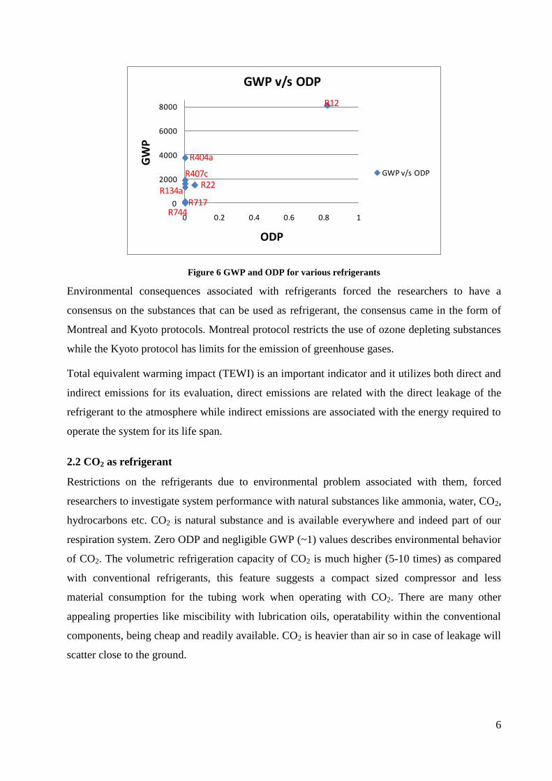
and ODP of natural refrigerants (R717, R744) are shown in figure 6 with other synthetic

refrigerants.

6

Figure 6 GWP and ODP for various refrigerants

Environmental consequences associated with refrigerants forced the researchers to have a

consensus on the substances that can be used as refrigerant, the consensus came in the form of

Montreal and Kyoto protocols. Montreal protocol restricts the use of ozone depleting substances

while the Kyoto protocol has limits for the emission of greenhouse gases.

Total equivalent warming impact (TEWI) is an important indicator and it utilizes both direct and

indirect emissions for its evaluation, direct emissions are related with the direct leakage of the

refrigerant to the atmosphere while indirect emissions are associated with the energy required to

operate the system for its life span.

2.2 CO2 as refrigerant

Restrictions on the refrigerants due to environmental problem associated with them, forced

researchers to investigate system performance with natural substances like ammonia, water, CO2,

hydrocarbons etc. CO2 is natural substance and is available everywhere and indeed part of our

respiration system. Zero ODP and negligible GWP (~1) values describes environmental behavior

of CO2. The volumetric refrigeration capacity of CO2 is much higher (5-10 times) as compared

with conventional refrigerants, this feature suggests a compact sized compressor and less

material consumption for the tubing work when operating with CO2. There are many other

appealing properties like miscibility with lubrication oils, operatability within the conventional

components, being cheap and readily available. CO2 is heavier than air so in case of leakage will

scatter close to the ground.

0

2000

4000

6000

8000

0 0.2 0.4 0.6 0.8 1

GW

P

ODP

GWP v/s ODP

GWP v/s ODP

R12

R404a

R22R134a

R717R744

R407c

7

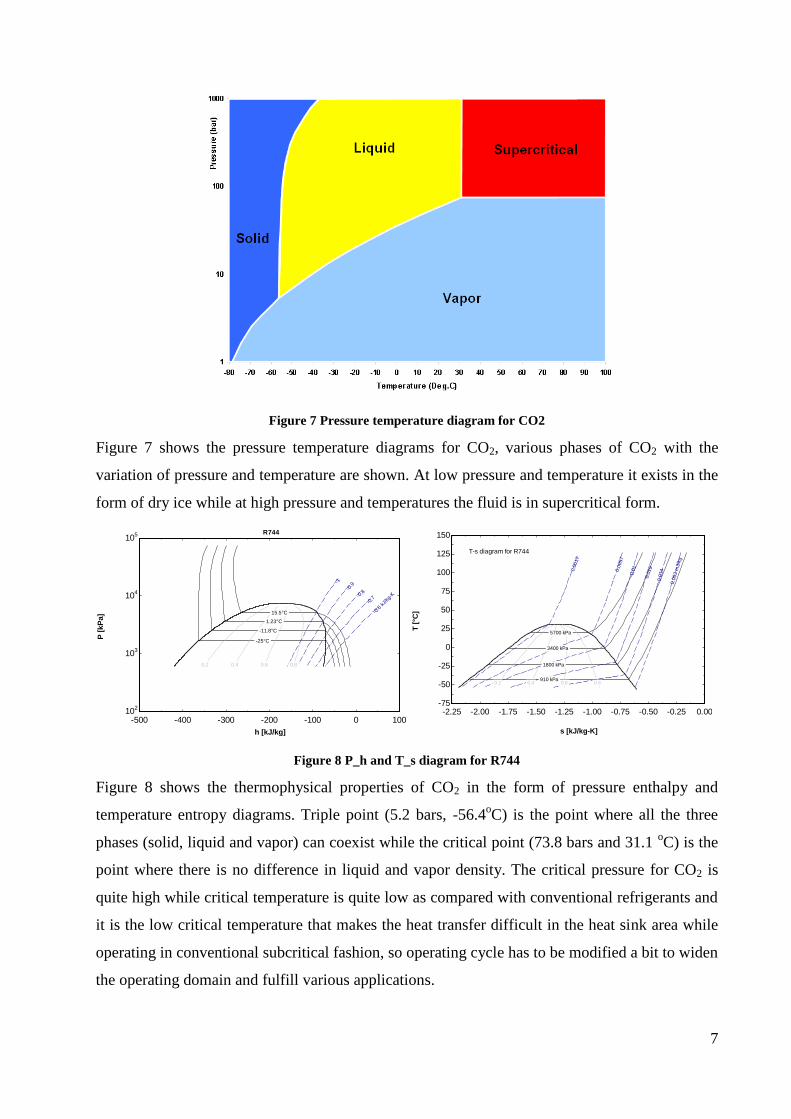
Figure 7 Pressure temperature diagram for CO2

Figure 7 shows the pressure temperature diagrams for CO2, various phases of CO2 with the

variation of pressure and temperature are shown. At low pressure and temperature it exists in the

form of dry ice while at high pressure and temperatures the fluid is in supercritical form.

Figure 8 P_h and T_s diagram for R744

Figure 8 shows the thermophysical properties of CO2 in the form of pressure enthalpy and

temperature entropy diagrams. Triple point (5.2 bars, -56.4oC) is the point where all the three

phases (solid, liquid and vapor) can coexist while the critical point (73.8 bars and 31.1 oC) is the

point where there is no difference in liquid and vapor density. The critical pressure for CO2 is

quite high while critical temperature is quite low as compared with conventional refrigerants and

it is the low critical temperature that makes the heat transfer difficult in the heat sink area while

operating in conventional subcritical fashion, so operating cycle has to be modified a bit to widen

the operating domain and fulfill various applications.

-500 -400 -300 -200 -100 0 10010

2

103

104

105

h [kJ/kg]

P [

kP

a] 15.5°C

1.23°C

-11.8°C

-25°C

0.2 0.4 0.6 0.8

-1

-0.9

-0.8

-0.7

-0.6

kJ/kg

-K

R744

-2.25 -2.00 -1.75 -1.50 -1.25 -1.00 -0.75 -0.50 -0.25 0.00-75

-50

-25

0

25

50

75

100

125

150

s [kJ/kg-K]

T [

°C]

5700 kPa

3400 kPa

1800 kPa

910 kPa 0.2 0.4 0.6 0.8

0.0

017

0.0

057

0.0

1

0.0

19

0.0

34

0.0

63 m

3/k

g

T-s diagram for R744

8

The trade name for the CO2 in the refrigeration industry is R744, where R is for refrigerant

application and the number 7 indicates the refrigerant family (Natural refrigerant) and the last

two digits 44 shows the molecular weight of CO2. The refrigerant CO2 used in the refrigeration

industry is basically a waste product of various industrial processes, and is extracted and

processed by different companies to be used as refrigerant.

2.2.1 History of CO2

CO2 is an old refrigerant and it is one of those which were used in the early application right

after the start of refrigeration industry. J&E Hall a British company, made the first two stage CO2

machine in 1889. CO2 was used in diverse applications and the most important application area

at that time was marine refrigeration where other refrigerants (like ammonia) could not be used

due to flammability and toxicity problems. Commonly stated problems at that time were,

High pressure containment with the available technology at that time.

Low COP and capacity loss at high heat rejection pressures.

Old working fluids were replaced by CFC’s which were introduced in 1930’s and 1940’s, they

were considered more safe than ammonia and SO2. Factors like low working pressure, better

efficiency, low cost assembly and aggressive marketing of CFC’s replaced CO2 as well.

As the problems associated with the CFC’s (Ozone Depletion) become clear, again there was

search for reliable refrigerants. In 1989 Professor Gustav Lorentzen devised a system utilizing

transcritical CO2 cycle, one promising application for that system was found in automobile air

conditioning (a dominant sector in refrigerant emission) which needs a non-toxic and non

flammable refrigerant. Professor Lorentzen compared the performance of CO2 with R-12 and

although CO2 was less efficient but several practical considerations made the actual efficiencies

of the two systems to be comparable. These were the results found by Professor Lorentzen and

others which again raised interest in CO2 as refrigerant, now a number of research projects (both

from industry and research sectors) are in process.

9

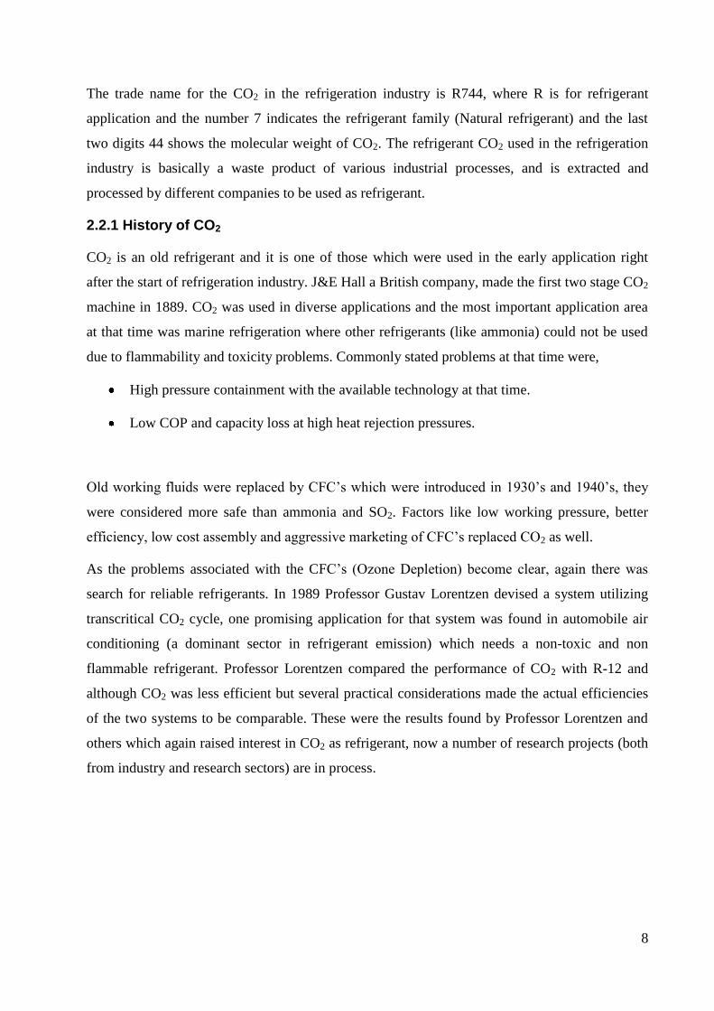
Figure 9 CO2 as refrigerant, usage history [4]

Figure 9 shows the early rise, decline and then revival in the usage of CO2 in twentieth century.

2.3 CO2 Transcritical cycle

The operating cycle with CO2 is simple vapor compression cycle however when working with

CO2, the low critical temperature limits the heat transfer process across the heat sink area. To

facilitate the heat transfer from CO2 across the heat sink, system has to be operated at above

critical conditions (31.1 oC and 73.8 bars). The resulting operating cycle will be called as

transcritical cycle, with supercritical conditions for CO2 across the heat sink and subcritical

conditions for CO2 across the heat source. Transcritical cycle was proposed for air conditioning

and heat pump applications by Prof. Gustav Lorentzen.

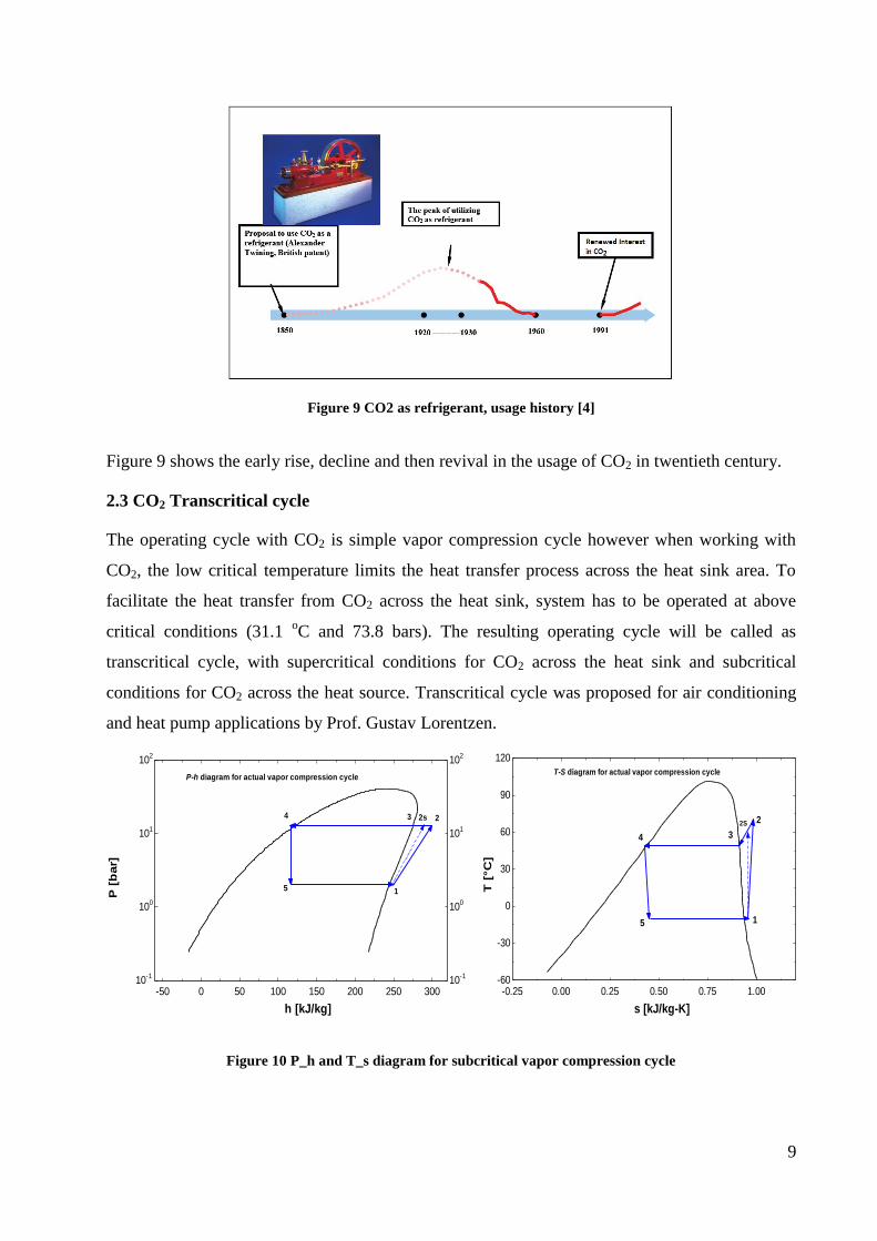
Figure 10 P_h and T_s diagram for subcritical vapor compression cycle

-50 0 50 100 150 200 250 30010

-1

100

101

102

10-1

100

101

102

h [kJ/kg]

P [

bar]

P-h diagram for actual vapor compression cycle

1

22s34

5

-0.25 0.00 0.25 0.50 0.75 1.00-60

-30

0

30

60

90

120

s [kJ/kg-K]

T [

°C

]

T-S diagram for actual vapor compression cycle

1

2

34

5

2S

10

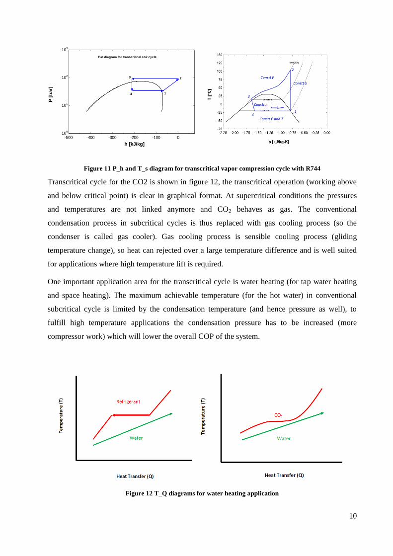
Figure 11 P_h and T_s diagram for transcritical vapor compression cycle with R744

Transcritical cycle for the CO2 is shown in figure 12, the transcritical operation (working above

and below critical point) is clear in graphical format. At supercritical conditions the pressures

and temperatures are not linked anymore and CO2 behaves as gas. The conventional

condensation process in subcritical cycles is thus replaced with gas cooling process (so the

condenser is called gas cooler). Gas cooling process is sensible cooling process (gliding

temperature change), so heat can rejected over a large temperature difference and is well suited

for applications where high temperature lift is required.

One important application area for the transcritical cycle is water heating (for tap water heating

and space heating). The maximum achievable temperature (for the hot water) in conventional

subcritical cycle is limited by the condensation temperature (and hence pressure as well), to

fulfill high temperature applications the condensation pressure has to be increased (more

compressor work) which will lower the overall COP of the system.

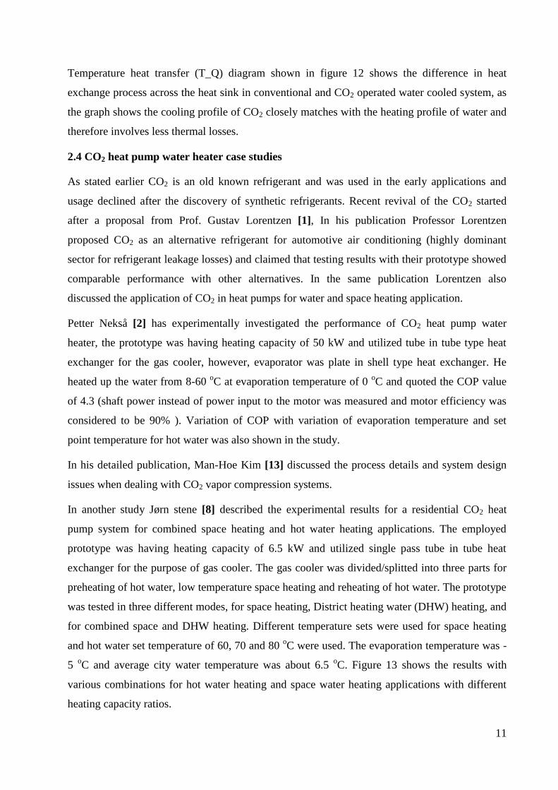
Figure 12 T_Q diagrams for water heating application

-500 -400 -300 -200 -100 010

0

101

102

103

h [kJ/kg]

P [

bar]

P-h diagram for transcritical co2 cycle

1

23

4

11

Temperature heat transfer (T_Q) diagram shown in figure 12 shows the difference in heat

exchange process across the heat sink in conventional and CO2 operated water cooled system, as

the graph shows the cooling profile of CO2 closely matches with the heating profile of water and

therefore involves less thermal losses.

2.4 CO2 heat pump water heater case studies

As stated earlier CO2 is an old known refrigerant and was used in the early applications and

usage declined after the discovery of synthetic refrigerants. Recent revival of the CO2 started

after a proposal from Prof. Gustav Lorentzen [1], In his publication Professor Lorentzen

proposed CO2 as an alternative refrigerant for automotive air conditioning (highly dominant

sector for refrigerant leakage losses) and claimed that testing results with their prototype showed

comparable performance with other alternatives. In the same publication Lorentzen also

discussed the application of CO2 in heat pumps for water and space heating application.

Petter Nekså [2] has experimentally investigated the performance of CO2 heat pump water

heater, the prototype was having heating capacity of 50 kW and utilized tube in tube type heat

exchanger for the gas cooler, however, evaporator was plate in shell type heat exchanger. He

heated up the water from 8-60 oC at evaporation temperature of 0

oC and quoted the COP value

of 4.3 (shaft power instead of power input to the motor was measured and motor efficiency was

considered to be 90% ). Variation of COP with variation of evaporation temperature and set

point temperature for hot water was also shown in the study.

In his detailed publication, Man-Hoe Kim [13] discussed the process details and system design

issues when dealing with CO2 vapor compression systems.

In another study Jørn stene [8] described the experimental results for a residential CO2 heat

pump system for combined space heating and hot water heating applications. The employed

prototype was having heating capacity of 6.5 kW and utilized single pass tube in tube heat

exchanger for the purpose of gas cooler. The gas cooler was divided/splitted into three parts for

preheating of hot water, low temperature space heating and reheating of hot water. The prototype

was tested in three different modes, for space heating, District heating water (DHW) heating, and

for combined space and DHW heating. Different temperature sets were used for space heating

and hot water set temperature of 60, 70 and 80 oC were used. The evaporation temperature was -

5 oC and average city water temperature was about 6.5

oC. Figure 13 shows the results with

various combinations for hot water heating and space water heating applications with different

heating capacity ratios.

12

Figure 13 Variation of COP with variation of set point temperature and heating capacity [8]

System performance with the variation of charge (amount of CO2) was studied by Hoghyun Cho

[10] who concluded that the cooling COP of the system reduced more significantly at

undercharged conditions as compared with overcharged conditions, furthermore, among the

considered alternatives (R22, R410A, R407C) with CO2 the system performance was most

sensitive with the refrigerant charge amount at under charged conditions.

In a recent study (2010) D. Leighton [11] presented the results for an air to water CO2 heat

pump, the system was utilizing plate type heat exchanger for the gas cooler. The main focus of

the study was to evaluate the performance of plate type heat exchanger which was used as a gas

cooler. The author calculated the effectiveness of the heat exchanger and then discussed the

results with various plots against the involved parameters (approach temperature, heating

capacity, and CO2 enthalpy).

E. Fornasieri [12] conducted tests on a water to water based CO2 heat pump which utilized

double plate type heat exchanger as a gas cooler and plate type heat exchanger as evaporator.

Double plate heat exchanger ensures no water contamination with lubricant oil in case of wall

failure. System performance was evaluated by varying the water inlet and set temperatures (for

gas cooler) and also by variation of evaporation temperature. Water inlet temperature for one

specific case was fixed while flow rate was varied to reach the desired set point temperature (60,

70 or 80 oC), for each value of water flow rate the gas cooler side pressure was varied with

expansion valve within the range of 80-112 bar. The maximum value of COP quoted in the study

was 3.9 when water was heated from 20-60 oC and high side pressure was 91 bars.

Another study was carried out by X.P. Zhang [15], the main objective of the study was to find

out relationship between optimum high side pressure, degree of superheat at the compressor inlet

13

and evaporation temperature. Both experimental and simulation approaches were used. Different

tests were done by varying these parameters and as per the stated results the optimum high side

pressure was more sensitive to the CO2 gas cooler outlet temperature while the degree of

superheat has negligible influence. The experimental setup was having counter flow tube in tube

type heat exchangers as evaporator and gas cooler.

14

15

Chapter No 3

3.1 System performance Evaluation

3.1.1 Coefficient of Performance (COP)

Performance of a refrigerating machine (be it a refrigerator or a heat pump) is measured by its

coefficient of performance (COP), this COP gives the information about how effectively that

machine is utilizing the supplied energy.

As in this specific case we are dealing with CO2 heat pump, the objective is to recover maximum

heat from the CO2 in the gas cooler by circulating water and mechanical work is supplied as

input to compressor to operate the system. The COP is defined as follows,

From second law of thermodynamics the COP of any reversible system operating between two

temperature limits is exactly same and completely independent of the involved refrigerant,

however these are the physical properties of the refrigerants that affect the system power

consumption through their influence on the thermodynamic losses.

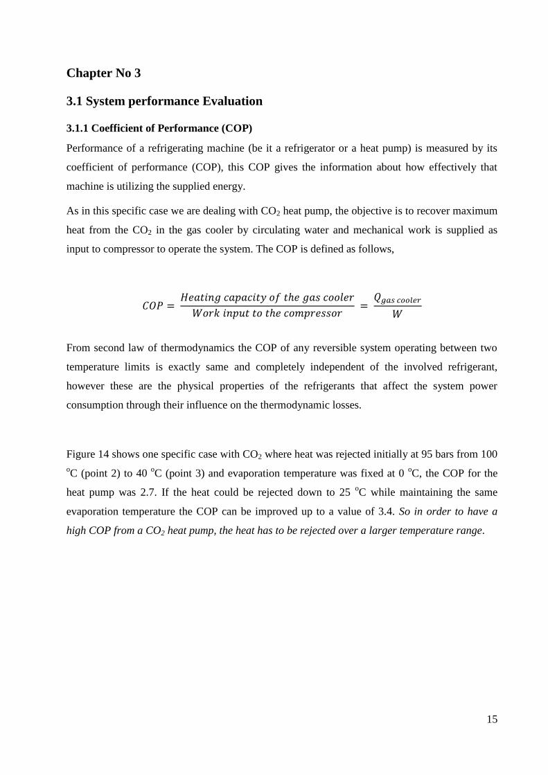
Figure 14 shows one specific case with CO2 where heat was rejected initially at 95 bars from 100

oC (point 2) to 40

oC (point 3) and evaporation temperature was fixed at 0

oC, the COP for the

heat pump was 2.7. If the heat could be rejected down to 25 oC while maintaining the same

evaporation temperature the COP can be improved up to a value of 3.4. So in order to have a

high COP from a CO2 heat pump, the heat has to be rejected over a larger temperature range.

16

Figure 14 Single stage CO2 heat pump cycle with decreasing gas cooler outlet temperature

3.2 References for Transcritical cycle

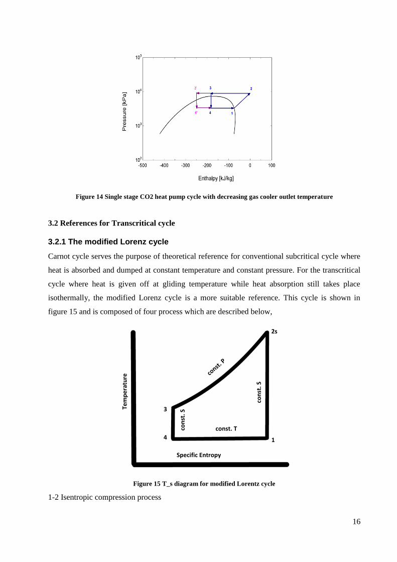
3.2.1 The modified Lorenz cycle

Carnot cycle serves the purpose of theoretical reference for conventional subcritical cycle where

heat is absorbed and dumped at constant temperature and constant pressure. For the transcritical

cycle where heat is given off at gliding temperature while heat absorption still takes place

isothermally, the modified Lorenz cycle is a more suitable reference. This cycle is shown in

figure 15 and is composed of four process which are described below,

Figure 15 T_s diagram for modified Lorentz cycle

1-2 Isentropic compression process

Tem

pe

ratu

re

Specific Entropy

const. T

con

st.S

con

st.S

1

2s

3

4

17

2-3 Constant pressure (gliding temperature) heat rejection process

3-4 Isentropic expansion process

4-1 Constant temperature heat absorption process

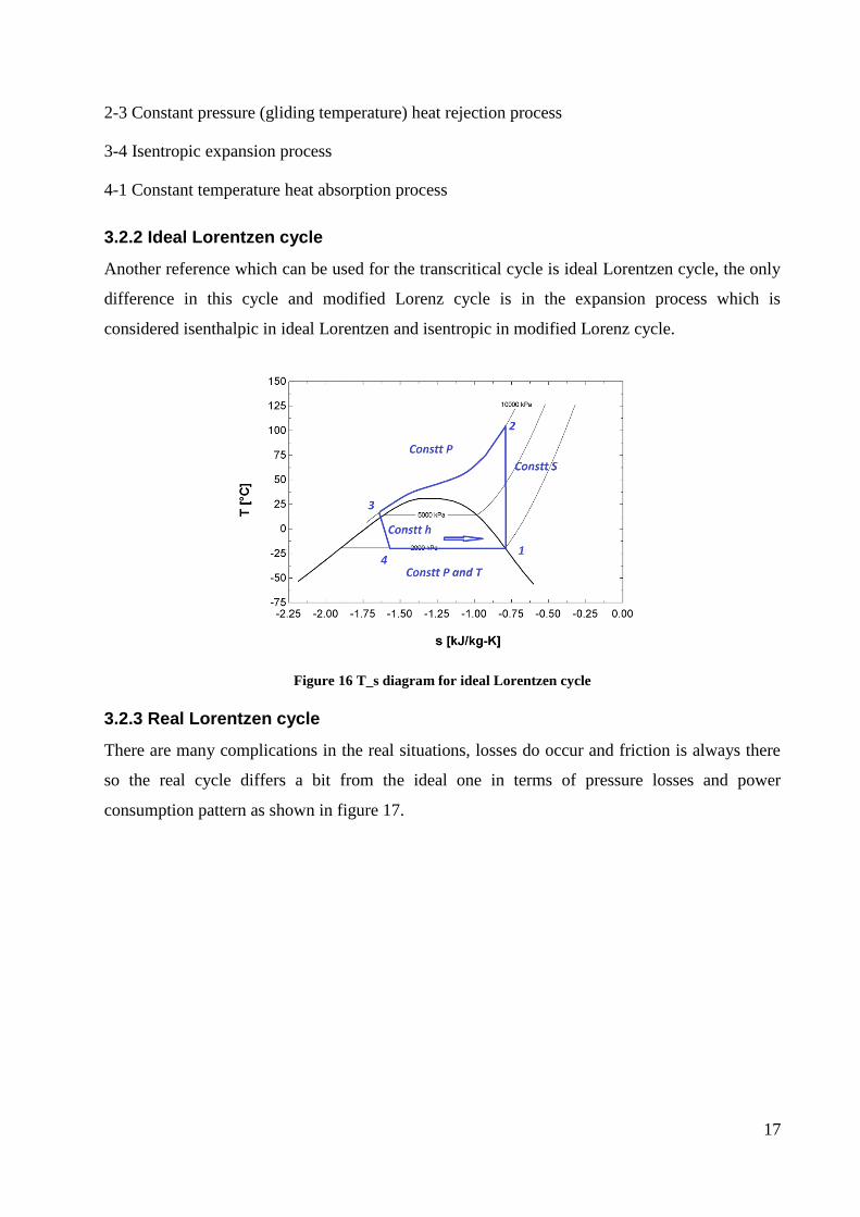
3.2.2 Ideal Lorentzen cycle

Another reference which can be used for the transcritical cycle is ideal Lorentzen cycle, the only

difference in this cycle and modified Lorenz cycle is in the expansion process which is

considered isenthalpic in ideal Lorentzen and isentropic in modified Lorenz cycle.

Figure 16 T_s diagram for ideal Lorentzen cycle

3.2.3 Real Lorentzen cycle

There are many complications in the real situations, losses do occur and friction is always there

so the real cycle differs a bit from the ideal one in terms of pressure losses and power

consumption pattern as shown in figure 17.

18

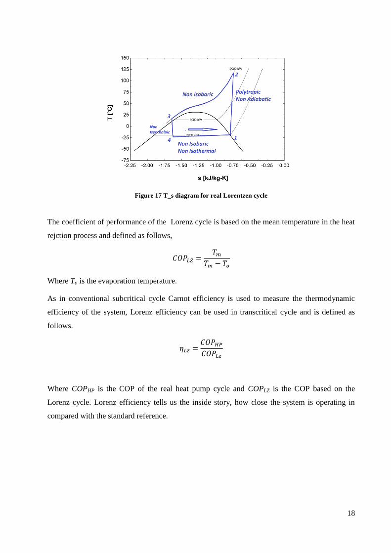
Figure 17 T_s diagram for real Lorentzen cycle

The coefficient of performance of the Lorenz cycle is based on the mean temperature in the heat

rejction process and defined as follows,

Where To is the evaporation temperature.

As in conventional subcritical cycle Carnot efficiency is used to measure the thermodynamic

efficiency of the system, Lorenz efficiency can be used in transcritical cycle and is defined as

follows.

Where COPHP is the COP of the real heat pump cycle and COPLZ is the COP based on the

Lorenz cycle. Lorenz efficiency tells us the inside story, how close the system is operating in

compared with the standard reference.

19

Chapter No 4

Heat Pump testing at KTH

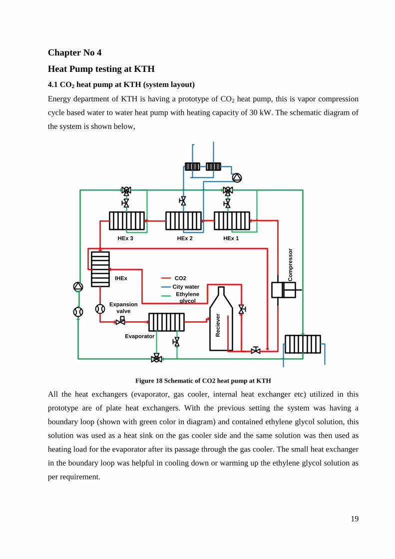
4.1 CO2 heat pump at KTH (system layout)

Energy department of KTH is having a prototype of CO2 heat pump, this is vapor compression

cycle based water to water heat pump with heating capacity of 30 kW. The schematic diagram of

the system is shown below,

HEx 1HEx 2HEx 3

IHEx

Evaporator

Expansion

valve

Re

cie

ve

r

Co

mp

res

so

rEthylene

glycol

City water

CO2

Figure 18 Schematic of CO2 heat pump at KTH

All the heat exchangers (evaporator, gas cooler, internal heat exchanger etc) utilized in this

prototype are of plate heat exchangers. With the previous setting the system was having a

boundary loop (shown with green color in diagram) and contained ethylene glycol solution, this

solution was used as a heat sink on the gas cooler side and the same solution was then used as

heating load for the evaporator after its passage through the gas cooler. The small heat exchanger

in the boundary loop was helpful in cooling down or warming up the ethylene glycol solution as

per requirement.

20

The gas cooler portion is divided into three heat exchangers, with heat exchanger No 1 and 3 for

the tap/district water heating application and heat exchanger No 2 (city water is used as heat sink

for this heat exchanger) for the space heating/floor heating. Any of the three heat exchangers (on

gas cooler) can be bypassed to operate system in various different modes.

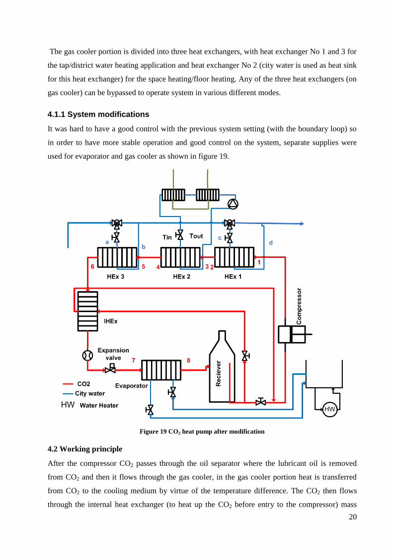
4.1.1 System modifications

It was hard to have a good control with the previous system setting (with the boundary loop) so

in order to have more stable operation and good control on the system, separate supplies were

used for evaporator and gas cooler as shown in figure 19.

Figure 19 CO2 heat pump after modification

4.2 Working principle

After the compressor CO2 passes through the oil separator where the lubricant oil is removed

from CO2 and then it flows through the gas cooler, in the gas cooler portion heat is transferred

from CO2 to the cooling medium by virtue of the temperature difference. The CO2 then flows

through the internal heat exchanger (to heat up the CO2 before entry to the compressor) mass

21

flow meter and expansion valve in its way to the evaporator. After the evaporator CO2 passes

through the receiver to the compressor and in this way completes the cycle.

4.2.1 Methodology

Heat pump was operated to heat up the water (to a set temperature) for tap water heating

application, system was operated at fixed evaporation temperature and gas cooler side pressure

was varied by changing the compressor speed (from 1050-1800 RPM) and adjustment of

expansion valve. Reading for temperatures, flow rate, pressures were taken when the system get

stable. These parameters were then used in Engineering Equation Solver (EES) to evaluate the

overall system performance (COP, Heating capacity, mass flow, etc).

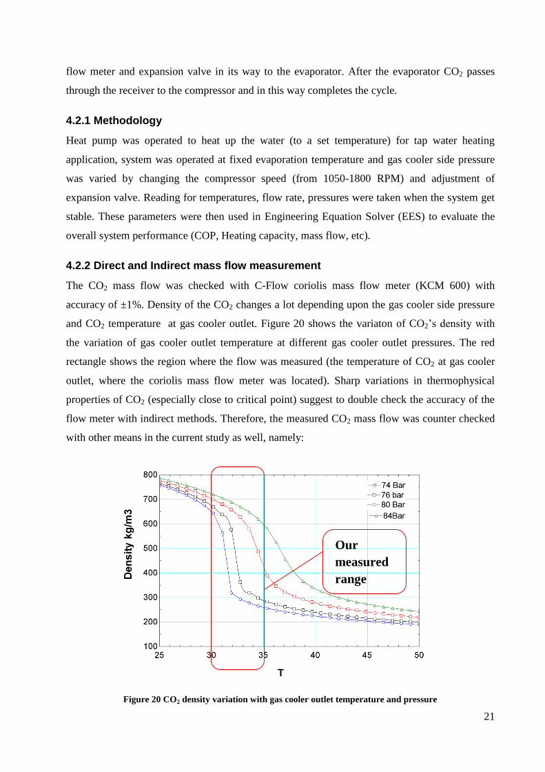
4.2.2 Direct and Indirect mass flow measurement

The CO2 mass flow was checked with C-Flow coriolis mass flow meter (KCM 600) with

accuracy of ±1%. Density of the CO2 changes a lot depending upon the gas cooler side pressure

and CO2 temperature at gas cooler outlet. Figure 20 shows the variaton of CO2’s density with

the variation of gas cooler outlet temperature at different gas cooler outlet pressures. The red

rectangle shows the region where the flow was measured (the temperature of CO2 at gas cooler

outlet, where the coriolis mass flow meter was located). Sharp variations in thermophysical

properties of CO2 (especially close to critical point) suggest to double check the accuracy of the

flow meter with indirect methods. Therefore, the measured CO2 mass flow was counter checked

with other means in the current study as well, namely:

Figure 20 CO2 density variation with gas cooler outlet temperature and pressure

Our

measured

range

22

Heat exchanger energy balance method

CO2 mass flow rate from the compressor manufacturer’s data

Energy balance on the gas cooler side is the one way for determining CO2 mass flow rate

indirectly, it utilizes following expressions;

The second indirect approach for getting mass flow rate of CO2 relies on the compressor

manufacturer’s data, with the information of swept volume of the compressor, the running speed,

property data along with the volumetric efficiency make it possible to determine the mass flow

rate with following expression.

Volumetric efficiency was calculated by using the curve fitting correlation (given by the

manufacturer) and is described below,

Where PR is the pressure ratio across the compressor

23

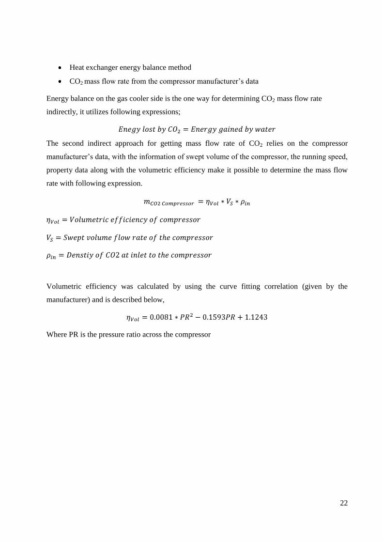
Figure 21 Variation of volumetric efficiency with gas cooler pressure

Volumetric efficiency decreases as pressure ratio across the compressor increases, the exact

trend for the variation of volumetric efficiency with variation in gas cooler pressure (while

evaporation pressure was constant) is shown in figure 21.

4.3 Results

The obtained results are discussed in detail in the following text and sub grouped in three groups

as described below.

Results for overall system performance (mainly COP, heating capacity etc)

Results for the component’s performance (Heat exchanger effectiveness)

Second law analysis for exergy destruction and entropy production in the system

4.3.1 Overall system performance from meter reading

Operating conditions

Heat pump was operated under various configurations, the imposed conditions and the obtained

results are discussed further in the following text.

Case A


Heat pump was operated to heat up the tap water to set point 60 oC and evaporation temperature

was varied (-5, 0 and 5oC) with only 1

ST Heat exchanger in operation.

24

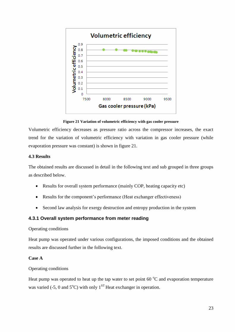
Figure 22 COP and heating capacity with the variation of gas cooler side pressure

Most of the observations were recorded during the summer period, temperature of the city water

was varying with the ambient temperature (in the range from 15-20 oC). Most of the previous

and current studies utilized tap water temperature of 60 oC, so we also tried to achieve the same

set temperature so the system performance can be compared under similar operating conditions.

From the graph it is clear that heating capacity and COP increases with the increase in

evaporation temperature, however, first heat exchanger is one part of whole gas cooler so

maximum achievable heating capacity and hence COP of the system is limited by the

geometrical constraints (I-e available heat transfer area).

Heating capacity seems to have negligible variation with the variation in the evaporation

temperature however COP of the system is sensitive to the evaporation temperature due to

variation in compressor power consumption (due to variation in pressure ratio).

0

5

10

15

20

25

30

0

0.5

1

1.5

2

2.5

3

3.5

7000 7500 8000 8500 9000 9500

CO

P

Gas cooler side pressure (kPa)

COP and heating capacity

COP at 0C evaporation COP at 5C evaporationCOP at -5C evaporation Heating capacity at 0C evaporationHeating capacity at 5C evaporation Heating capacity at -5C evaporation

He

ati

ng

cap

aci

ty (

kW

)

25

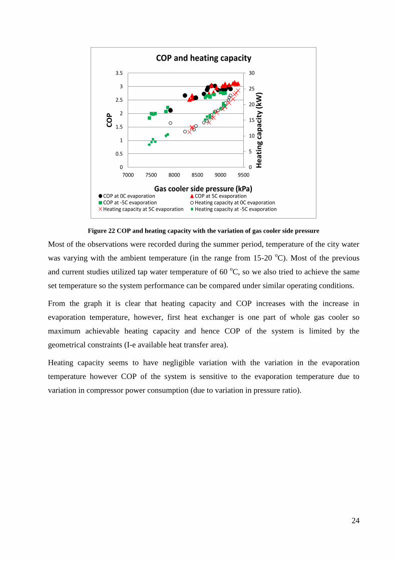
Figure 23 T_h diagram for 1st Heat exchanger

Cooling profile of CO2 and heating profile of water for this specific case (for 1st heat exchanger

in operation) is shown in figure 23. Cooling and heating curves (for CO2 and water respectively)

are quite close to each other, better matching of cooling and heating cooling curves results in

improved heat transfer.

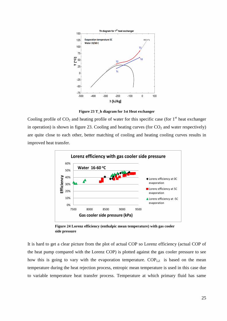
It is hard to get a clear picture from the plot of actual COP so Lorenz efficiency (actual COP of

the heat pump compared with the Lorenz COP) is plotted against the gas cooler pressure to see

how this is going to vary with the evaporation temperature. COPLZ is based on the mean

temperature during the heat rejection process, entropic mean temperature is used in this case due

to variable temperature heat transfer process. Temperature at which primary fluid has same

0%

10%

20%

30%

40%

50%

60%

7500 8000 8500 9000 9500

Effi

cie

ncy


Lorenz efficiency with gas cooler side pressure

Lorenz efficiency at 0Cevaporation


Lorenz efficiency at -5Cevaporation

Water 16-60 oC

Figure 24 Lorenz efficiency (enthalpic mean temperature) with gas cooler

side pressure

26

exergy value both at the inlet and outlet of the heat exchanger is called as entropic mean

temperature, thermodynamically

Variation of Lorenz efficiency with the variation of gas cooler side pressure at three different

evaporation temperatures is shown graphically in figure 24. Higher values for Lorenz efficiency

were noticed at lower evaporation temperature.

One explanation, COPLZ is dependent on mean temperature of CO2 (in the heat rejection process)

and on the source temperature, if all the conditions (except evaporation temperature) are

maintained then logically COPLZ should have a lower value at low evaporation temperatures.

Actual COP of the system is also decreased when operating at low evaporation temperature,

however, COPLZ is found to be more sensitive with evaporation temperature so as a result higher

values for Lorenz efficiency were found at lower evaporation temperature.

Case B


Only for tap water heating application (for set point of 50 oC) at varying (-5, 0 and 5

oC)

evaporation temperatures with 3RD

heat exchanger in operation only.

Results

27

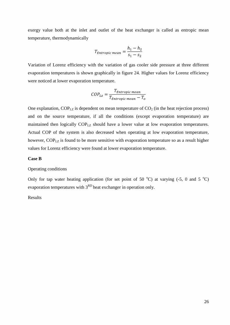
Figure 25 COP and heating capacity variation with gas cooler side pressure

Compared with first heat exchanger less heat transfer area is available in third heat exchanger,

water flow needs to be regulated (compared with case A) to reach the same set point of 60 oC,

furthermore CO2 leaves the gas cooler at higher temperature (as less heat is recovered from it)

and in this way eventually affect the operating pressure in the system. So to avoid all such

practical complications water set point of 50 oC was used in this specific case.

Variation of COP and heating capacity with gas cooler side pressure variation at three different

evaporation temperatures is shown in figure 25, trend is similar like the first heat exchanger, the

heating capacity and COP increases with the increase in evaporation temperature.

0

5

10

15

20

25

0

0.5

1

1.5

2

2.5

3

3.5

7000 7500 8000 8500 9000 9500

CO

P


COP and heating capacity

COP at 0C evaporation COP at -5C evaporation

COP at 5C evaporation Heating capacity at 0C evaporation

Heating capacity at 5C evaporation Heating capacity at-5C evaporation

He

atin

gca

pac

ity

(kW

)

Water 19/50 oC

28

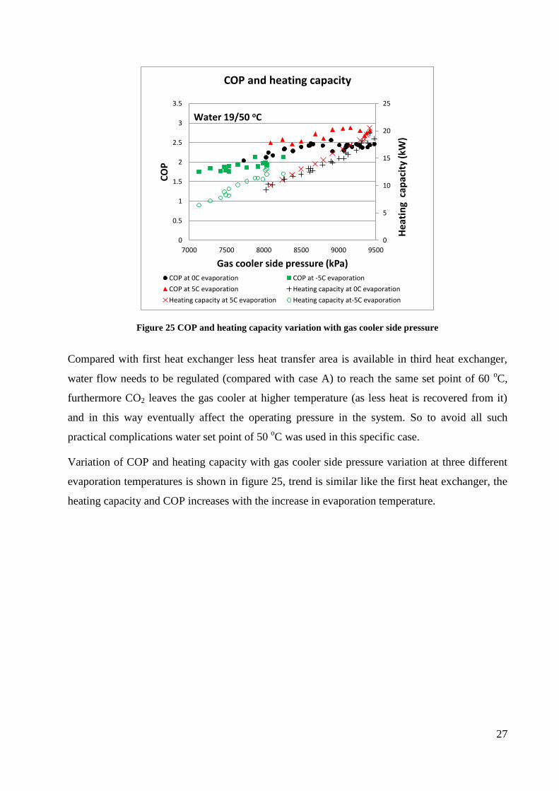
Figure 26 T_h diagram for 3rd heat exchanger

Temperature enthalpy diagram for this case is shown in figure 26 Compared to case A the two

curves (cooling curve for CO2 and heating curve for water) are a bit far from each other, means

more energy losses and less efficient heating process.

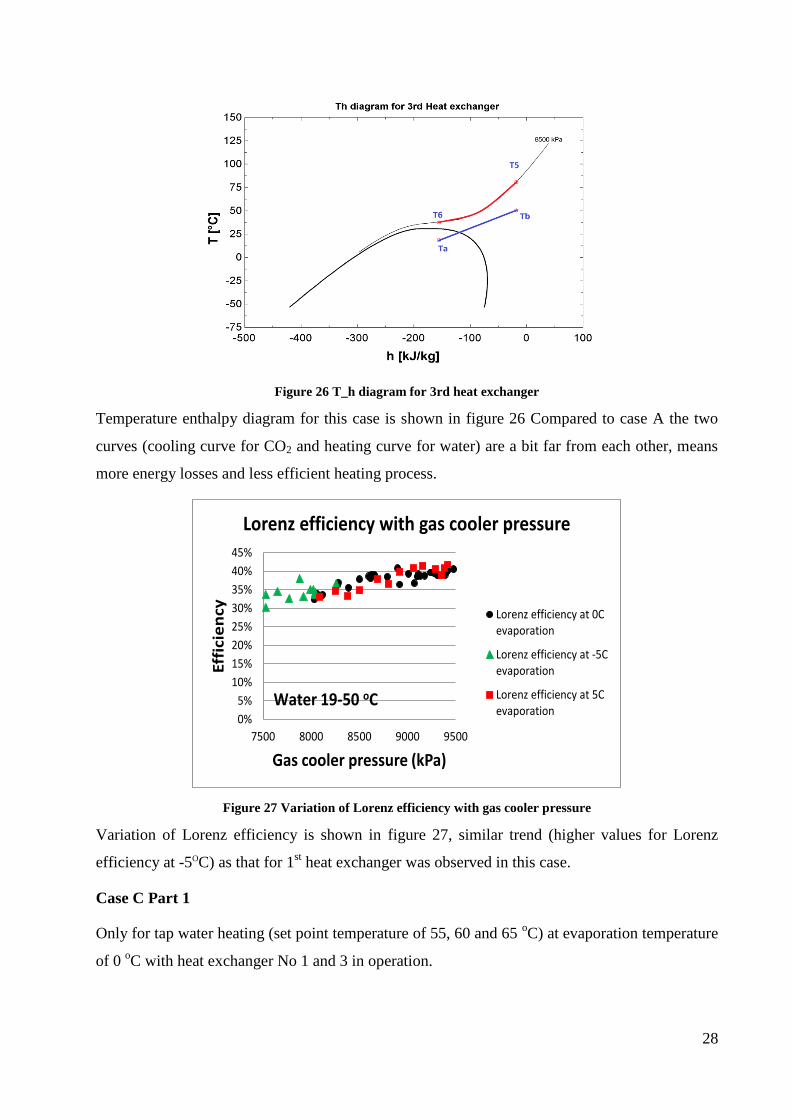
Figure 27 Variation of Lorenz efficiency with gas cooler pressure

Variation of Lorenz efficiency is shown in figure 27, similar trend (higher values for Lorenz

efficiency at -5OC) as that for 1st heat exchanger was observed in this case.

Case C Part 1

Only for tap water heating (set point temperature of 55, 60 and 65 oC) at evaporation temperature

of 0 oC with heat exchanger No 1 and 3 in operation.

0%

5%

10%

15%

20%

25%

30%

35%

40%

45%

7500 8000 8500 9000 9500

Eff

icie

ncy

Gas cooler pressure (kPa)

Lorenz efficiency with gas cooler pressure




Water 19-50 oC

29

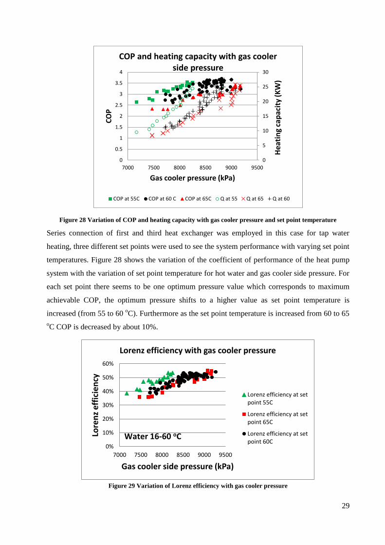
Figure 28 Variation of COP and heating capacity with gas cooler pressure and set point temperature

Series connection of first and third heat exchanger was employed in this case for tap water

heating, three different set points were used to see the system performance with varying set point

temperatures. Figure 28 shows the variation of the coefficient of performance of the heat pump

system with the variation of set point temperature for hot water and gas cooler side pressure. For

each set point there seems to be one optimum pressure value which corresponds to maximum

achievable COP, the optimum pressure shifts to a higher value as set point temperature is

increased (from 55 to 60 oC). Furthermore as the set point temperature is increased from 60 to 65

oC COP is decreased by about 10%.


0

5

10

15

20

25

30

0

0.5

1

1.5

2

2.5

3

3.5

4

7000 7500 8000 8500 9000 9500

CO

P


COP and heating capacity with gas cooler side pressure

COP at 55C COP at 60 C COP at 65C Q at 55 Q at 65 Q at 60

He

atin

gca

pac

ity

(KW

)

0%

10%

20%

30%

40%

50%

60%

7000 7500 8000 8500 9000 9500

Lore

nz

effi

cie

ncy



Lorenz efficiency at setpoint 55C



Water 16-60 oC

30

Figure 29 shows the variation of Lorenz efficiency with gas cooler side pressure, the trend shows

linear increase in achieved values with the increment in pressure. Compared with previous cases

in this case CO2 was leaving the gas cooler at lower temperatures, possibility to further cool CO2

compared with previous two cases (more energy was recovered) could be the one of the reasons

for having higher values for Lorenz efficiency in this specific case.

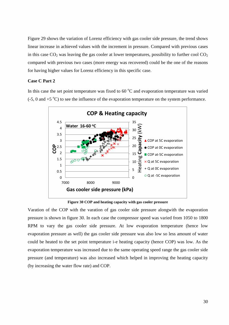
Case C Part 2

In this case the set point temperature was fixed to 60 oC and evaporation temperature was varied

(-5, 0 and +5 oC) to see the influence of the evaporation temperature on the system performance.

Figure 30 COP and heating capacity with gas cooler pressure

Varation of the COP with the varation of gas cooler side pressure alongwith the evaporation

pressure is shown in figure 30. In each case the compressor speed was varied from 1050 to 1800

RPM to vary the gas cooler side pressure. At low evaporation temperature (hence low

evaporation pressure as well) the gas cooler side pressure was also low so less amount of water

could be heated to the set point temperature i-e heating capacity (hence COP) was low. As the

evaporation temperature was increased due to the same operating speed range the gas cooler side

pressure (and temperature) was also increased which helped in improving the heating capacity

(by increasing the water flow rate) and COP.

0

5

10

15

20

25

30

35

0

0.5

1

1.5

2

2.5

3

3.5

4

4.5

7000 8000 9000

CO

P


COP & Heating capacity

COP at 5C evaporation

COP at 0C evaporation

COP at-5C evaporation

Q at 5C evaporation

Q at 0C evaporation

Q at -5C evaporation

Hea

tin

gC

apac

ity

(kW

)Water 16-60 oC

31

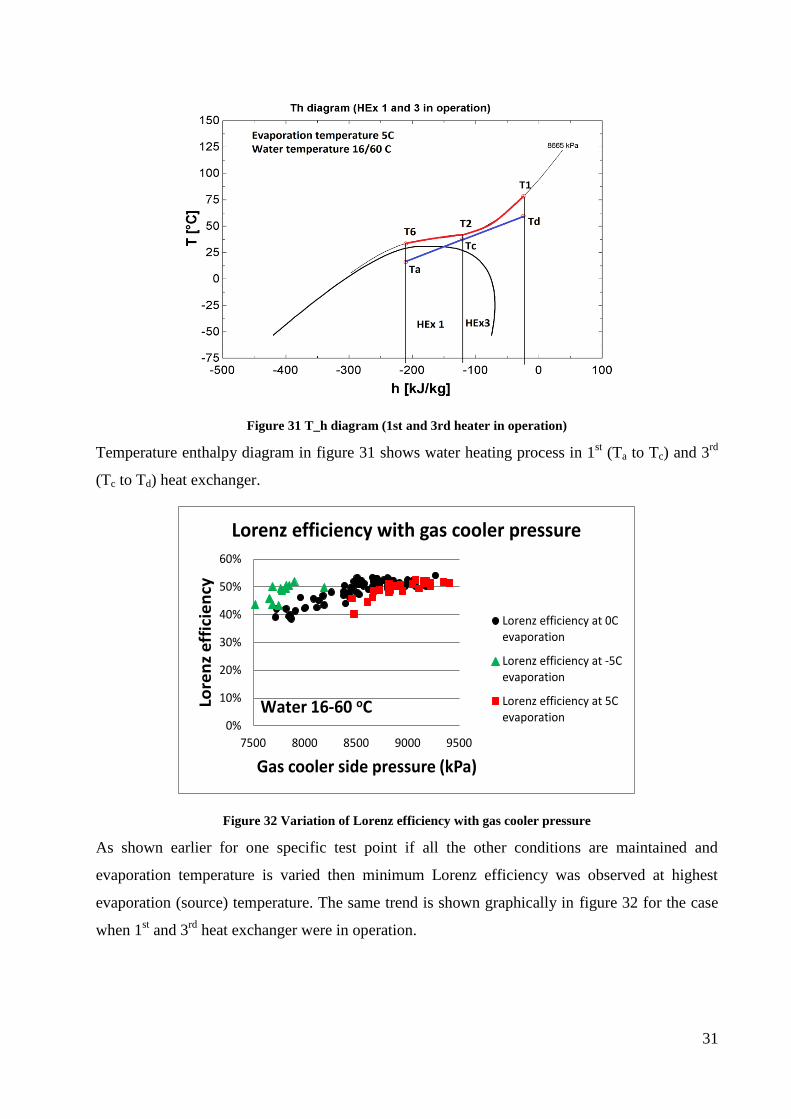
Figure 31 T_h diagram (1st and 3rd heater in operation)

Temperature enthalpy diagram in figure 31 shows water heating process in 1st (Ta to Tc) and 3

rd

(Tc to Td) heat exchanger.


As shown earlier for one specific test point if all the other conditions are maintained and

evaporation temperature is varied then minimum Lorenz efficiency was observed at highest

evaporation (source) temperature. The same trend is shown graphically in figure 32 for the case

when 1st and 3

rd heat exchanger were in operation.

0%

10%

20%

30%

40%

50%

60%

7500 8000 8500 9000 9500

Lore

nz

eff

icie

ncy






Water 16-60 oC

32

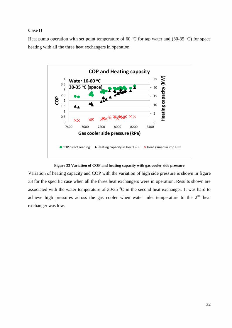
Case D

Heat pump operation with set point temperature of 60 oC for tap water and (30-35

oC) for space

heating with all the three heat exchangers in operation.

Figure 33 Variation of COP and heating capacity with gas cooler side pressure

Variation of heating capacity and COP with the variation of high side pressure is shown in figure

33 for the specific case when all the three heat exchangers were in operation. Results shown are

associated with the water temperature of 30/35 oC in the second heat exchanger. It was hard to

achieve high pressures across the gas cooler when water inlet temperature to the 2nd

heat

exchanger was low.

0

5

10

15

20

25

0

0.5

1

1.5

2

2.5

3

3.5

4

7400 7600 7800 8000 8200 8400

CO

P


COP and Heating capacity

COP direct reading Heating capacity in Hex 1 + 3 Heat gained in 2nd HEx

He

atin

gca

pac

ity

(kW

)

Water 16-60 oC30-35 oC (space)

33

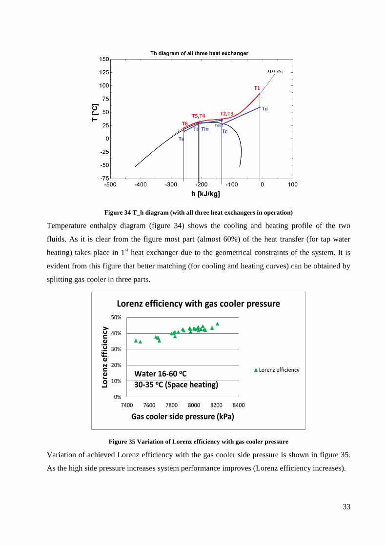
Figure 34 T_h diagram (with all three heat exchangers in operation)

Temperature enthalpy diagram (figure 34) shows the cooling and heating profile of the two

fluids. As it is clear from the figure most part (almost 60%) of the heat transfer (for tap water

heating) takes place in 1st heat exchanger due to the geometrical constraints of the system. It is

evident from this figure that better matching (for cooling and heating curves) can be obtained by

splitting gas cooler in three parts.


Variation of achieved Lorenz efficiency with the gas cooler side pressure is shown in figure 35.

As the high side pressure increases system performance improves (Lorenz efficiency increases).

0%

10%

20%

30%

40%

50%

7400 7600 7800 8000 8200 8400

Lore

nz

eff

icie

ncy



Lorenz efficiencyWater 16-60 oC30-35 oC (Space heating)

34

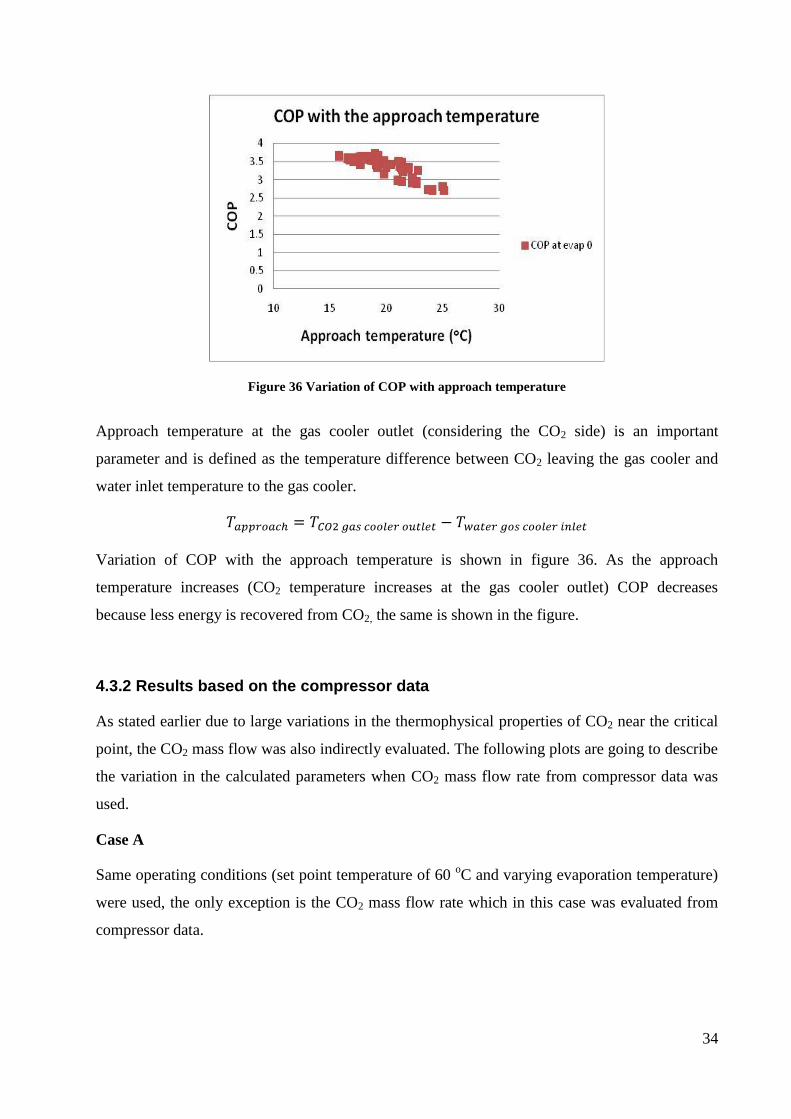
Figure 36 Variation of COP with approach temperature

Approach temperature at the gas cooler outlet (considering the CO2 side) is an important

parameter and is defined as the temperature difference between CO2 leaving the gas cooler and

water inlet temperature to the gas cooler.

Variation of COP with the approach temperature is shown in figure 36. As the approach

temperature increases (CO2 temperature increases at the gas cooler outlet) COP decreases

because less energy is recovered from CO2, the same is shown in the figure.

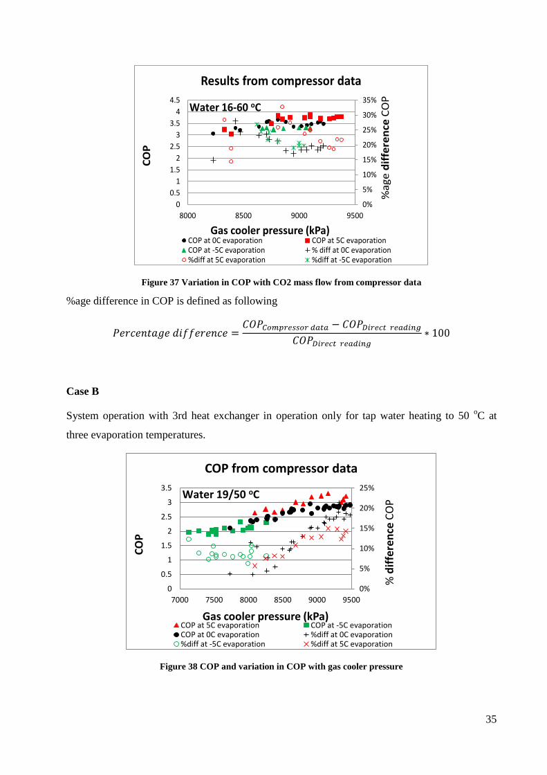
4.3.2 Results based on the compressor data

As stated earlier due to large variations in the thermophysical properties of CO2 near the critical

point, the CO2 mass flow was also indirectly evaluated. The following plots are going to describe

the variation in the calculated parameters when CO2 mass flow rate from compressor data was

used.

Case A

Same operating conditions (set point temperature of 60 oC and varying evaporation temperature)

were used, the only exception is the CO2 mass flow rate which in this case was evaluated from

compressor data.

35

Figure 37 Variation in COP with CO2 mass flow from compressor data

%age difference in COP is defined as following

Case B

System operation with 3rd heat exchanger in operation only for tap water heating to 50 oC at

three evaporation temperatures.

Figure 38 COP and variation in COP with gas cooler pressure

0%

5%

10%

15%

20%

25%

30%

35%

0

0.5

1

1.5

2

2.5

3

3.5

4

4.5

8000 8500 9000 9500

CO

P


Results from compressor data

COP at 0C evaporation COP at 5C evaporationCOP at -5C evaporation % diff at 0C evaporation%diff at 5C evaporation %diff at -5C evaporation

%a

ge d

iffe

ren

ceC

OP

Water 16-60 oC

0%

5%

10%

15%

20%

25%

0

0.5

1

1.5

2

2.5

3

3.5

7000 7500 8000 8500 9000 9500

CO

P


COP from compressor data

COP at 5C evaporation COP at -5C evaporationCOP at 0C evaporation %diff at 0C evaporation%diff at -5C evaporation %diff at 5C evaporation

% d

iffe

ren

ceC

OP

Water 19/50 oC

36

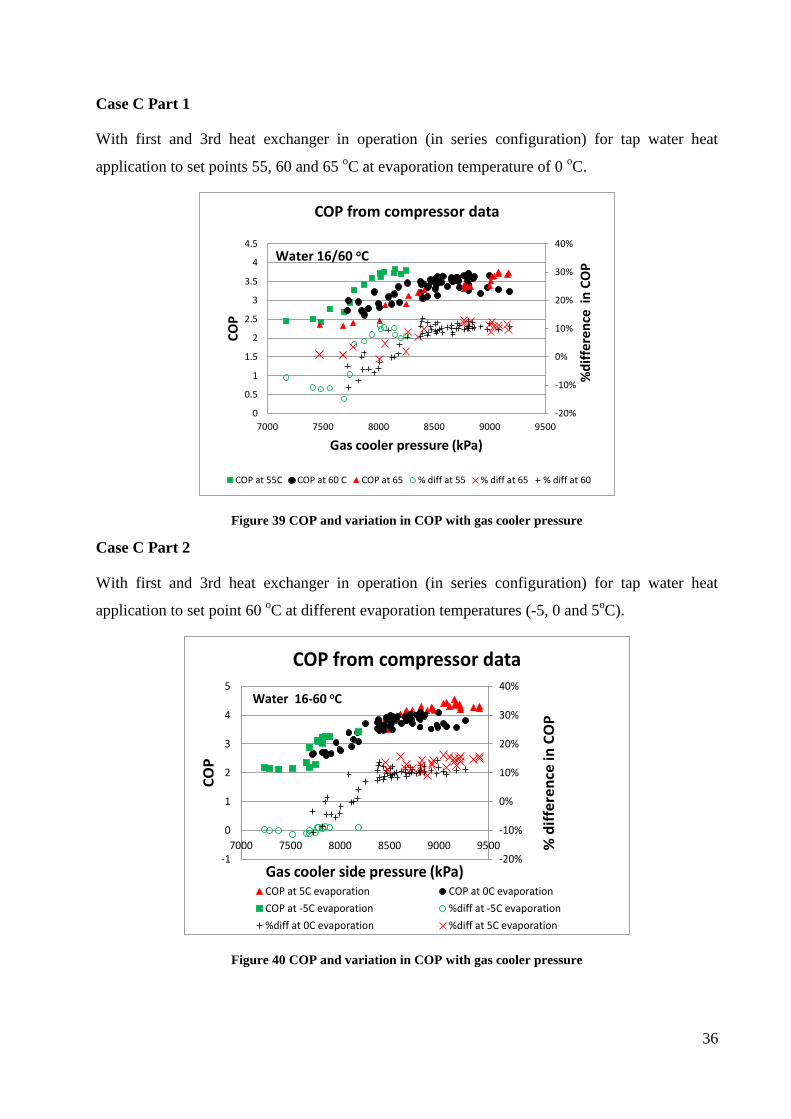
Case C Part 1

With first and 3rd heat exchanger in operation (in series configuration) for tap water heat

application to set points 55, 60 and 65 oC at evaporation temperature of 0

oC.


Case C Part 2

With first and 3rd heat exchanger in operation (in series configuration) for tap water heat

application to set point 60 oC at different evaporation temperatures (-5, 0 and 5

oC).


-20%

-10%

0%

10%

20%

30%

40%

0

0.5

1

1.5

2

2.5

3

3.5

4

4.5

7000 7500 8000 8500 9000 9500

CO

P



COP at 55C COP at 60 C COP at 65 % diff at 55 % diff at 65 % diff at 60

%d

iffe

ren

cein

CO

P

Water 16/60 oC

-20%

-10%

0%

10%

20%

30%

40%

-1

0

1

2

3

4

5

7000 7500 8000 8500 9000 9500

CO

P



COP at 5C evaporation COP at 0C evaporation

COP at -5C evaporation %diff at -5C evaporation

%diff at 0C evaporation %diff at 5C evaporation

% d

iffe

ren

cein

CO

P

Water 16-60 oC

37

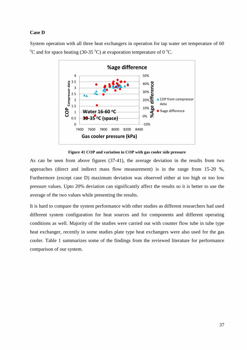
Case D

System operation with all three heat exchangers in operation for tap water set temperature of 60

oC and for space heating (30-35

oC) at evaporation temperature of 0

oC.

Figure 41 COP and variation in COP with gas cooler side pressure

As can be seen from above figures (37-41), the average deviation in the results from two

approaches (direct and indirect mass flow measurement) is in the range from 15-20 %,

Furthermore (except case D) maximum deviation was observed either at too high or too low

pressure values. Upto 20% deviation can significantly affect the results so it is better to use the

average of the two values while presenting the results.

It is hard to compare the system performance with other studies as different researchers had used

different system configuration for heat sources and for components and different operating

conditions as well. Majority of the studies were carried out with counter flow tube in tube type

heat exchanger, recently in some studies plate type heat exchangers were also used for the gas

cooler. Table 1 summarizes some of the findings from the reviewed literature for performance

comparison of our system.

-10%

0%

10%

20%

30%

40%

50%

0

0.5

1

1.5

2

2.5

3

3.5

4

7400 7600 7800 8000 8200 8400

%A

ge d

iffe

ren

ce


%age difference

COP from compressordata

%age difference

CO

PC

om

pre

sso

r d

ata

Water 16-60 oC30-35 oC (space)

38

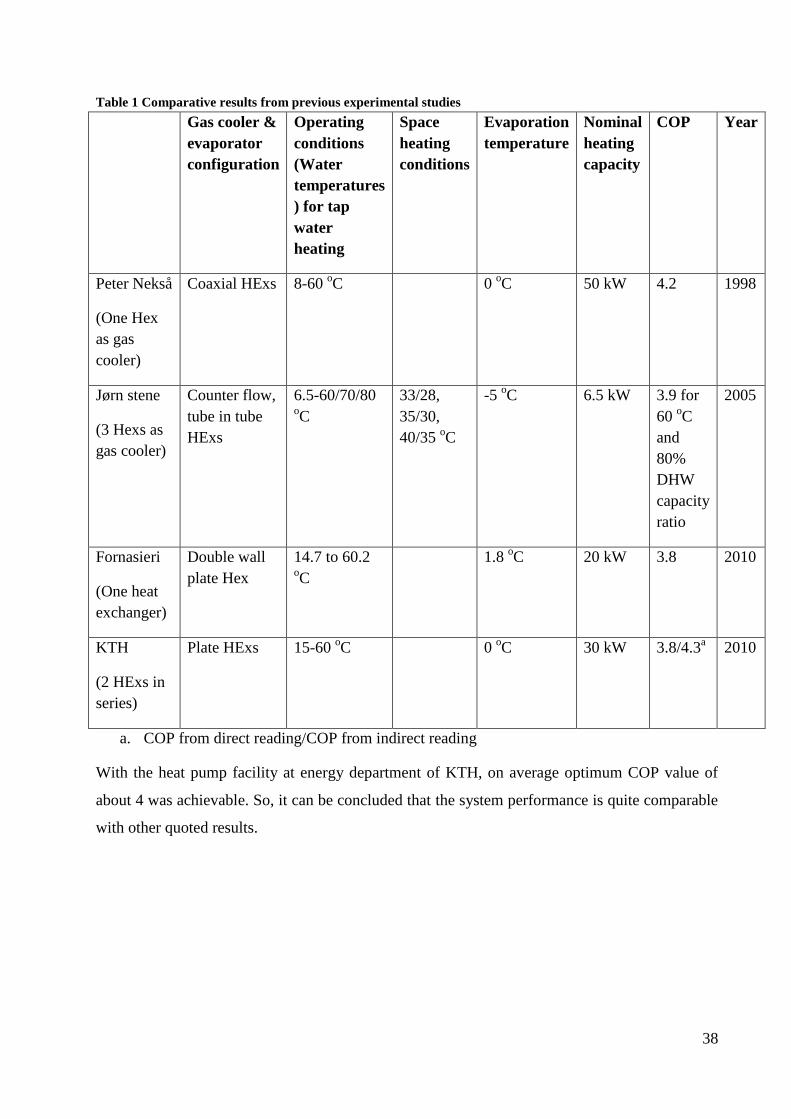
Table 1 Comparative results from previous experimental studies

Gas cooler &

evaporator

configuration

Operating

conditions

(Water

temperatures

) for tap

water

heating

Space

heating

conditions

Evaporation

temperature

Nominal

heating

capacity

COP Year

Peter Nekså

(One Hex

as gas

cooler)

Coaxial HExs 8-60 oC 0

oC 50 kW 4.2 1998

Jørn stene

(3 Hexs as

gas cooler)

Counter flow,

tube in tube

HExs

6.5-60/70/80 oC

33/28,

35/30,

40/35 oC

-5 oC 6.5 kW 3.9 for

60 oC

and

80%

DHW

capacity

ratio

2005

Fornasieri

(One heat

exchanger)

Double wall

plate Hex

14.7 to 60.2 oC

1.8 oC 20 kW 3.8 2010

KTH

(2 HExs in

series)

Plate HExs 15-60 oC 0

oC 30 kW 3.8/4.3

a 2010

a. COP from direct reading/COP from indirect reading

With the heat pump facility at energy department of KTH, on average optimum COP value of

about 4 was achievable. So, it can be concluded that the system performance is quite comparable

with other quoted results.

39

4.3.3 Results for the components testing

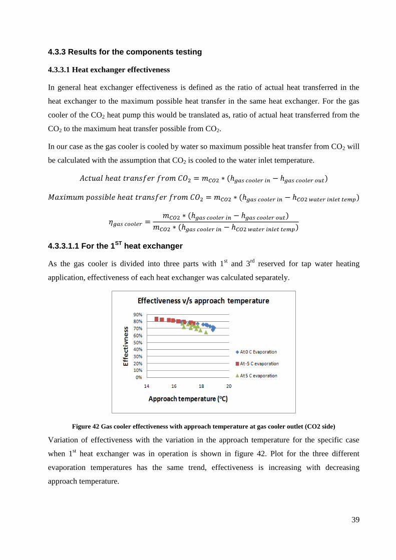
4.3.3.1 Heat exchanger effectiveness

In general heat exchanger effectiveness is defined as the ratio of actual heat transferred in the

heat exchanger to the maximum possible heat transfer in the same heat exchanger. For the gas

cooler of the CO2 heat pump this would be translated as, ratio of actual heat transferred from the

CO2 to the maximum heat transfer possible from CO2.

In our case as the gas cooler is cooled by water so maximum possible heat transfer from CO2 will

be calculated with the assumption that CO2 is cooled to the water inlet temperature.

4.3.3.1.1 For the 1ST heat exchanger

As the gas cooler is divided into three parts with 1st and 3

rd reserved for tap water heating

application, effectiveness of each heat exchanger was calculated separately.

Figure 42 Gas cooler effectiveness with approach temperature at gas cooler outlet (CO2 side)

Variation of effectiveness with the variation in the approach temperature for the specific case

when 1st heat exchanger was in operation is shown in figure 42. Plot for the three different

evaporation temperatures has the same trend, effectiveness is increasing with decreasing

approach temperature.

40

Figure 43 Gas cooler effectiveness with variation in heating capacity

Plot for the effectiveness with heating capacity (figure 43) shows effectiveness increases with

increase in heating capacity, higher heating capacities were obtained at high temperatures and

pressures for CO2. One possible explanation is, at high CO2 temperatures more water can be

heated to the set point temperature so this increased mass flow (hence increased velocity as well)

for water suggests improved convective heat transfer on the water side.

Figure 44 cooling and heating profiles with variation in approach temperature

Cooling profile of CO2 and heating profile of water is shown in figure 44, as can be seen the

increase in approach temperature (high CO2 temperature at gas cooler outlet) there comes a pinch

point which limits the heat exchange between the two fluids and hence reduces the effectiveness.

41

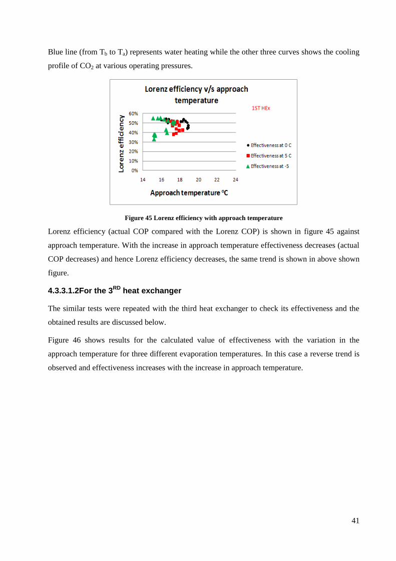
Blue line (from Tb to Ta) represents water heating while the other three curves shows the cooling

profile of CO2 at various operating pressures.

Figure 45 Lorenz efficiency with approach temperature

Lorenz efficiency (actual COP compared with the Lorenz COP) is shown in figure 45 against

approach temperature. With the increase in approach temperature effectiveness decreases (actual

COP decreases) and hence Lorenz efficiency decreases, the same trend is shown in above shown

figure.

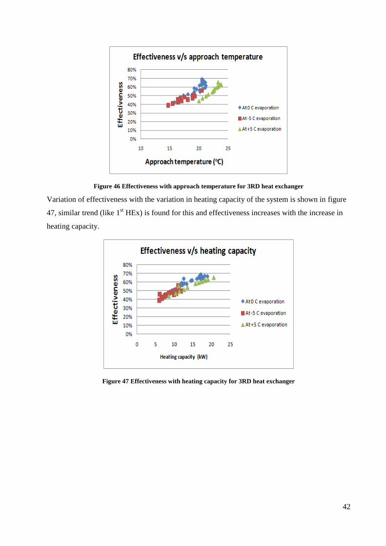
4.3.3.1.2For the 3RD heat exchanger

The similar tests were repeated with the third heat exchanger to check its effectiveness and the

obtained results are discussed below.

Figure 46 shows results for the calculated value of effectiveness with the variation in the

approach temperature for three different evaporation temperatures. In this case a reverse trend is

observed and effectiveness increases with the increase in approach temperature.

42

Figure 46 Effectiveness with approach temperature for 3RD heat exchanger

Variation of effectiveness with the variation in heating capacity of the system is shown in figure

47, similar trend (like 1st HEx) is found for this and effectiveness increases with the increase in

heating capacity.

Figure 47 Effectiveness with heating capacity for 3RD heat exchanger

43

Figure 48 Variation of Lorenz efficiency with approach temperature

Figure 49 Variation of cooling and heating profile with approach temperature

Cooling and heating curves for this specific case are shown in figure 49. In general effectiveness

increases by reducing approach temperature, however reverse trend is observed for the case

when 3RD

heat exchanger was in operation. For better understanding cooling and heating curves

for the two cases (with 1ST

and 3RD

heat exchanger) were plotted under various imposed

operating conditions and it was finally concluded that it was the interaction of cooling and

heating curve and not the approach temperature which affects the achieved values for

effectiveness

T1

T2 Ta

Tb

44

4.4.4 Second law analysis of the transcritical cycle

First law analysis is simple and shows an overall picture for the system performance while

second law analysis makes it possible to find out contribution of each component in

irreversibility. Second law analysis of the system is therefore done to see how effectively the

components are doing their tasks and see which components need to be improved. Following two

approaches were utilized in the second law analysis,

a. Exergy balance method: to find out exergy destruction in the components.

b. Entropy contribution method: to investigate entropy production in the components.

Where ho and so are the enthalpy and entropy values at atmospheric temperature of 0 oC. Change

of exergy in a component is calculated as,

And exergetic efficiency is calculated by,

Utilized expressions are summarized in table below and were found from [16] for the calculation

of exergy destruction and entropy production in the components.

Exergy balance method Entropy balance

method

Gas cooler Exergy supplied:

Exergy recovered:

Evaporator Exergy supplied:

Exergy recovered:

45

Compressor Exergy supplied:

Exergy recovered:

Expansion

valve

Exergy loss:

Losses in exergy value and produced entropies were calculated by considering the expansion

process as isenthalpic (having constant enthalpy) and furthermore losses occurred within the

pipes were considered negligible. Figure 50-52 shows the contribution of four components in

overall entropy production. In this particular case compressor and expansion valve are the major

sources of entropy production in the system.

Figure 50 Entropy produced in expansion valve and compressor

0%

10%

20%

30%

40%

50%

60%

70%

6500 7500 8500 9500

Co

ntr

ibu

tio

n


Entropy produced in expansion valve

From EV at 0 evap

From EV at -5 evap

From EV at 5 evap

0%

10%

20%

30%

40%

50%

60%

70%

6500 7500 8500 9500

Co

ntr

ibu

tio

n


Entropy produced in compressor

From compressor at 0evap

From compressor at -5evap

From compressor at 5evap

46

Figure 51 Entropy produced in gas cooler and evaporator

Figure 52 Entropy production in components against gas cooler pressure

Exergy efficiency of the components (gas cooler, expansion valve, evaporator and compressor)

is shown in figure 53 and 54. Results showed most of (about 40%) the exergy losses occur in

compressor, contribution from evaporator and expansion valve was almost same (about 23%

from each) and was less than compressor, while least value for exergy losses was found for the

gas cooler and was about 14% of total losses. On average exergetic efficiency for the compressor

was about 70% (at 5 C evaporation) while for evaporator it was 22%, so there is more room for

imporvement in evaporator as compared with compressor.

0%

1%

2%

3%

4%

5%

6%

6500 7500 8500 9500

Co

ntr

ibu

tio

n


Entropy produced in gas cooler

From gas cooler at 0 evap

From gas cooler at -5 evap

From gas cooler at 5 evap

0%

1%

2%

3%

4%

5%

6%

6000 7000 8000 9000

Co

ntr

ibu

tio

n


Entropy produced in evaporator

From evaporator at 0evap

From evaporator at -5

From evaporator at 5evap

0%

20%

40%

60%

80%

100%

86

10

86

60

86

70

88

20

88

20

88

30

88

80

89

30

89

30

89

50

90

50

90

80

91

10

91

60

91

60

91

80

92

20

93

50

Entropy production in components

Entropy production in expansion valve Entropy production in compressorEntropy production in evaporator Entropy production in gas cooler

Entr

op

y P

rod

uct

ion


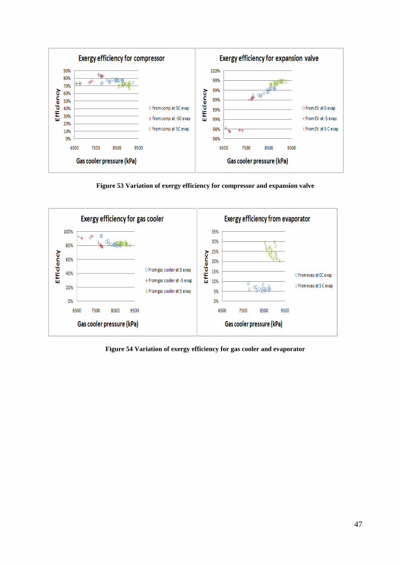
47

Figure 53 Variation of exergy efficiency for compressor and expansion valve

Figure 54 Variation of exergy efficiency for gas cooler and evaporator

48

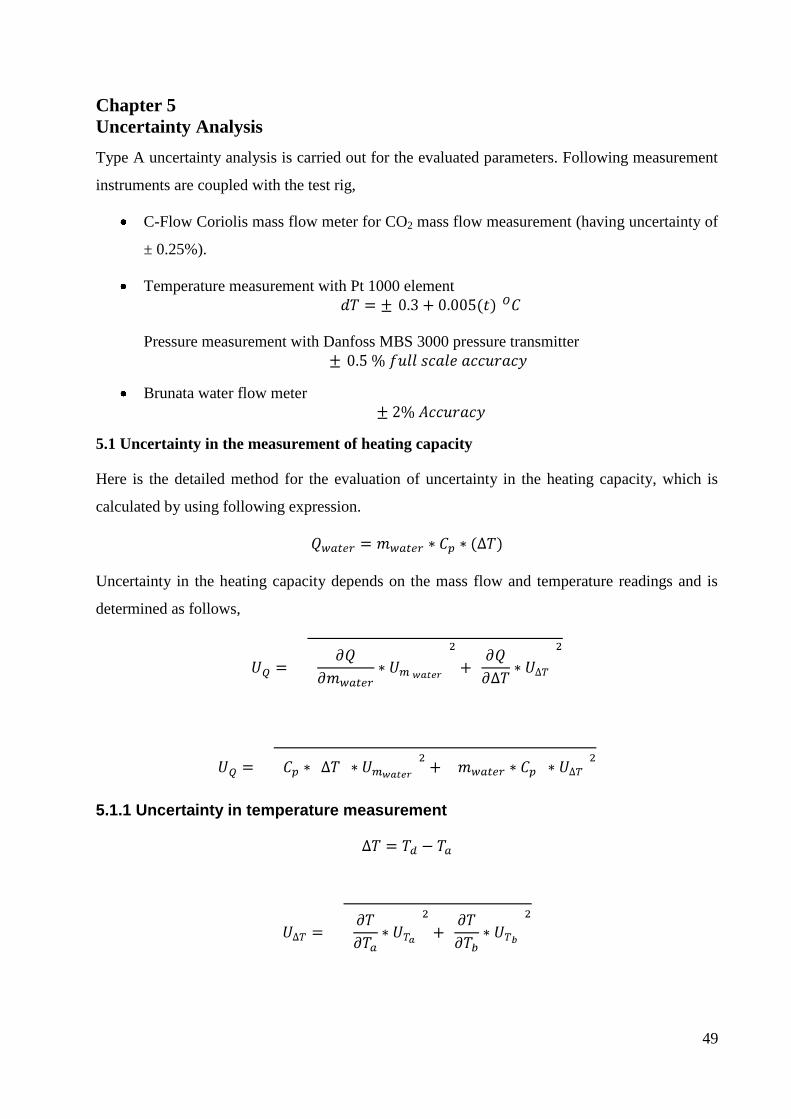
49

Chapter 5

Uncertainty Analysis

Type A uncertainty analysis is carried out for the evaluated parameters. Following measurement

instruments are coupled with the test rig,

C-Flow Coriolis mass flow meter for CO2 mass flow measurement (having uncertainty of

± 0.25%).

Temperature measurement with Pt 1000 element

Pressure measurement with Danfoss MBS 3000 pressure transmitter

Brunata water flow meter

5.1 Uncertainty in the measurement of heating capacity

Here is the detailed method for the evaluation of uncertainty in the heating capacity, which is

calculated by using following expression.

Uncertainty in the heating capacity depends on the mass flow and temperature readings and is

determined as follows,

5.1.1 Uncertainty in temperature measurement

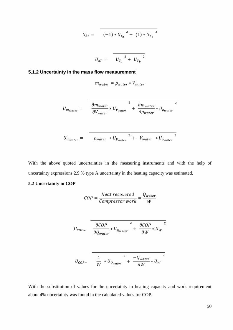
50

5.1.2 Uncertainty in the mass flow measurement

With the above quoted uncertainties in the measuring instruments and with the help of

uncertainty expressions 2.9 % type A uncertainty in the heating capacity was estimated.

5.2 Uncertainty in COP

With the substitution of values for the uncertainty in heating capacity and work requirement

about 4% uncertainty was found in the calculated values for COP.

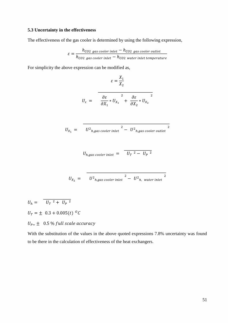
51

5.3 Uncertainty in the effectiveness

The effectiveness of the gas cooler is determined by using the following expression,

For simplicity the above expression can be modified as,

With the substitution of the values in the above quoted expressions 7.8% uncertainty was found

to be there in the calculation of effectiveness of the heat exchangers.

52

53

Conclusion

Overall system analysis of the CO2 heat pump has been discussed in this study, direct and

indirect approaches were used for observing CO2 mass flow rate. Various conditions were

imposed (by varying system arrangement or by varying operating parameters) to check the

system performance. Effectiveness of the heat exchangers (on the gas cooler side) was calculated

to have an inner look in the involved heat transfer process. Finally second law analysis was

carried out to check the sources of irreversibilities and entropy production in the system.

Engineering equation solver (EES) was used to get the property data and for the calculation

purpose.

Testing results showed comparative system performance (COP of about 4) with most of

the studies under similar imposed operating conditions.

On average about 20% deviation was observed in the results from two approaches (direct

and indirect mass flow readings), it was further observed that maximum deviation

occurred at higher pressures.

Results for the effectiveness made it clear that while dealing with CO2 overall matching

of cooling and heating curve is more influential parameter than the approach temperature

alone (at gas cooler outlet on CO2 side) for better understanding the obtained results.

Second law analysis showed compressor and expansion valve are the main sources for

the exergy destruction and entropy production in the system, however minimum value for

the exergetic efficiency was found for the evaporator.

54

55

References

1. G. Lorentzen, Revival of Carbon dioxide as a refrigerant, 1994, International Journal of

refrigeration.

2. Petter. Nekså, CO2 heat pump systems,2000,International Journal of refrigeration, 421-

427.

3. Mohanraj.M, Environment friendly alternative to halogenated refrigerants A review,

2009, Green house gas control, 108-119.

4. Sarkar.J, Natural refrigerant based subcritical and transcritical cycles for high

temperature heating,2007,International journal of refrigeration, 3-10.

5. Pearson.andy, Carbon dioxide new uses for an old refrigerant,2005, International journal

of refrigeration, 1140-48.

6. Cecchinato.Luca, CO2 as refrigerant for tap water heat pumps a comparison with

traditional solution, 2005, International Journal of refrigeration, 1250-1258.

7. http://www.brighthub.com/engineering/mechanical/articles/965.aspx

8. Jørn.Stene, Residential CO2 heat pump system for combined space heating and hot water

heating, 2005, International Journal of refrigeration, 1259-1265.

9. Willys.Adriansyah, Combined air conditioning and tap water heating plant using CO2 as

refrigerant, 2004, Energy and buildings, 690-695.

10. Honghyun .Cho, Effects of refrigerant charge amount on the performance of transcritical

CO2 heat pump, 2005, International Journal of Refrigeration, 1266-1273.

11. D. Leighton, Compact brazed plate type heat exchangers for CO2 heat pump water heater,

2010, 9TH

IIR Gustav Lorentzen conference.

12. E.Fornasieri, A carbon dioxide domestic hot water heat pump with double wall plate heat

exchanger gas cooler, 2010, 9TH

IIR Gustav Lorentzen conference.

13. Man.Hoe. Kim, Fundamental process and system design issues in CO2 vapor

compression systems, 2004, Progress in energy and combustion science, 119-174.

14. www.R744.com

15. X.P. Zhang, Theoritical and experimental studies on optimum heat rejection pressure for

CO2 heat pump system, 2010, Applied thermal engineering, 2537-2544.

16. Amir F, Second law analysis of transcritical CO2 refrigeration cycle, Energy conversion

and Management, 2003, 2269-2281.

17. www.ehpa.org

http://www.brighthub.com/engineering/mechanical/articles/965.aspx

http://www.r744.com/

http://www.ehpa.org/

Documents

Experimental investigation of heat recovery from R744 ...418902/FULLTEXT01.pdf · Experimental investigation of heat ... Experimental investigation of heat recovery from R744 based