Embed Size (px)
Citation preview
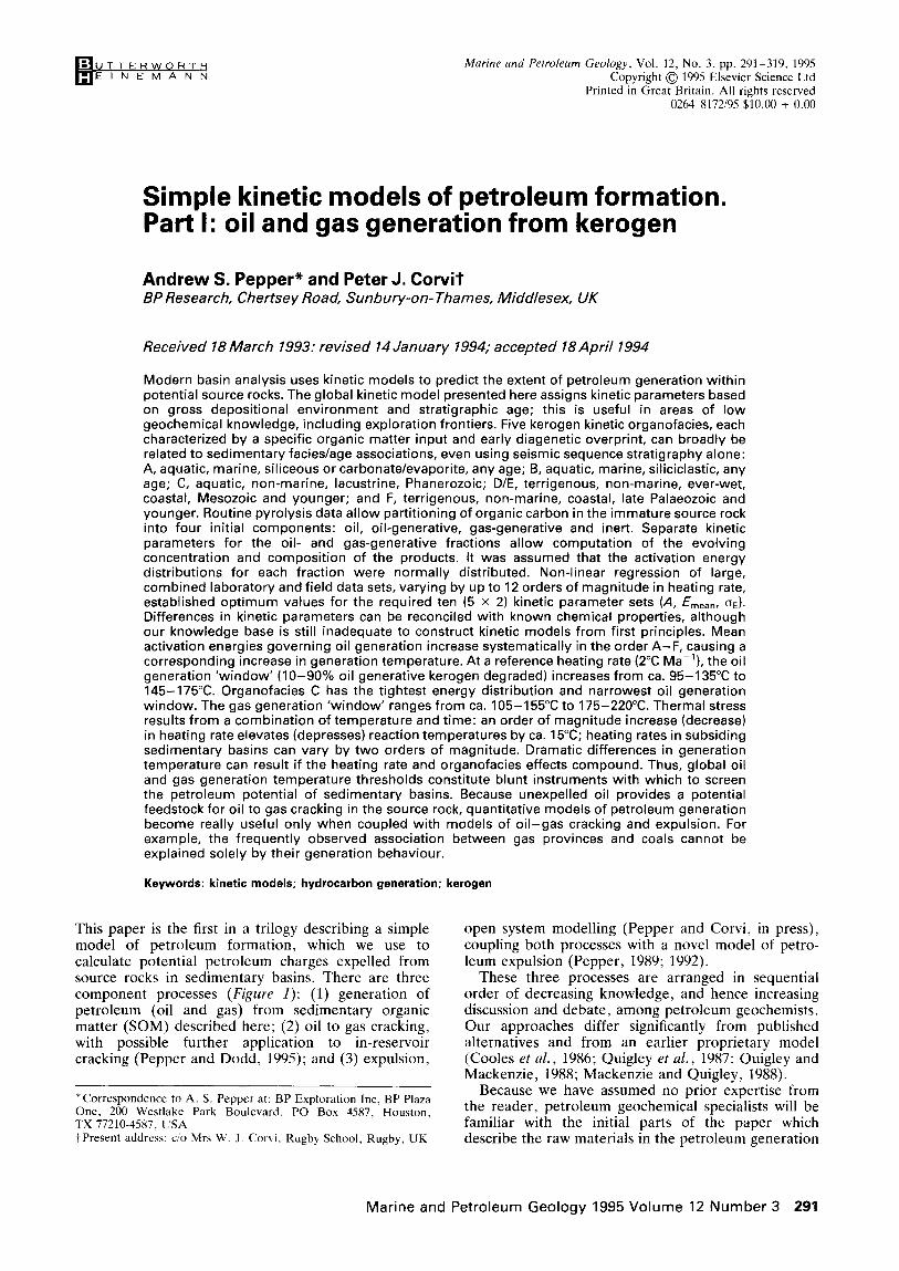
Marine and Petroleum Geology, Vol. 12, No. 3, pp. 291-319, 1995 Copyright 0 1995 Elsevier Science Ltd
Printed in Great Britain. All rights reserved 026~8172/95 $10.00 + 0.00
Simple kinetic models of petroleum formation. Part I: oil and gas generation from kerogen
Andrew S. Pepper* and Peter J. Corvit BP Research, Chertsey Road, Sunbury-on- Thames, Middlesex, UK
Received 18 illarch 1993: revised 14January 7994; accepted 18 April 1994
Modern basin analysis uses kinetic models to predict the extent of petroleum generation within potential source rocks. The global kinetic model presented here assigns kinetic parameters based on gross depositional environment and stratigraphic age; this is useful in areas of low geochemical knowledge, including exploration frontiers. Five kerogen kinetic organofacies, each characterized by a specific organic matter input and early diagenetic overprint, can broadly be related to sedimentary facies/age associations, even using seismic sequence stratigraphy alone: A, aquatic, marine, siliceous or carbonate/evaporite, any age; 6, aquatic, marine, siliciclastic, any age; C, aquatic, non-marine, lacustrine, Phanerozoic; D/E, terrigenous, non-marine, ever-wet, coastal, Mesozoic and younger; and F, terrigenous, non-marine, coastal, late Palaeozoic and younger. Routine pyrolysis data allow partitioning of organic carbon in the immature source rock into four initial components: oil, oil-generative, gas-generative and inert. Separate kinetic parameters for the oil- and gas-generative fractions allow computation of the evolving concentration and composition of the products. It was assumed that the activation energy distributions for each fraction were normally distributed. Non-linear regression of large, combined laboratory and field data sets, varying by up to 12 orders of magnitude in heating rate, established optimum values for the required ten (5 x 2) kinetic parameter sets (A, E,,,,, IJ~). Differences in kinetic parameters can be reconciled with known chemical properties, although our knowledge base is still inadequate to construct kinetic models from first principles. Mean activation energies governing oil generation increase systematically in the order A-F, causing a corresponding increase in generation temperature. At a reference heating rate (2°C Ma-‘), the oil generation ‘window’ (IO-90% oil generative kerogen degraded) increases from ca. 95-135°C to 145-175°C. Organofacies C has the tightest energy distribution and narrowest oil generation window. The gas generation ‘window’ ranges from ca. 105-155°C to 175-220°C. Thermal stress results from a combination of temperature and time: an order of magnitude increase (decrease) in heating rate elevates (depresses) reaction temperatures by ca. 15°C; heating rates in subsiding sedimentary basins can vary by two orders of magnitude. Dramatic differences in generation temperature can result if the heating rate and organofacies effects compound. Thus, global oil and gas generation temperature thresholds constitute blunt instruments with which to screen the petroleum potential of sedimentary basins. Because unexpelled oil provides a potential feedstock for oil to gas cracking in the source rock, quantitative models of petroleum generation become really useful only when coupled with models of oil-gas cracking and expulsion. For example, the frequently observed association between gas provinces and coals cannot be explained solely by their generation behaviour.
Keywords: kinetic models; hydrocarbon generation; kerogen
This paper is the first in a trilogy describing a simple model of petroleum formation, which we use to calculate potential petroleum charges expelled from source rocks in sedimentary basins. There are three component processes (Figure 1): (1) generation of petroleum (oil and gas) from sedimentary organic matter (SOM) described here; (2) oil to gas cracking, with possible further application to in-reservoir cracking (Pepper and Dodd, 1995); and (3) expulsion,
*Correspondence to A. S. Pepper at: BP Exploration Inc, BP Plaza One, 200 Westlakc Park Boulevard. PO Box 4587, Houston, TX 77210-4587, USA I-Present address: cio Mrs W. J. Corvi, Rugby School, Rugby, UK
open system modelling (Pepper and Corvi, in press), coupling both processes with a novel model of petro- leum expulsion (Pepper, 1989; 1992).
These three processes are arranged in sequential order of decreasing knowledge, and hence increasing discussion and debate, among petroleum geochemists. Our approaches differ significantly from published alternatives and from an earlier proprietary model (Cooles et al., 1986; Quigley et al., 1987; Quigley and Mackenzie, 1988; Mackenzie and Quigley, 1988).
Because we have assumed no prior expertise from the reader, petroleum geochemical specialists will be familiar with the initial parts of the paper which describe the raw materials in the petroleum generation
Marine and Petroleum Geology 1995 Volume 12 Number 3 291

KEROGEN U&O)
Mid INITIAL REACTIVE (C,,a”)
GENERATION I/ I I
EXPULSION
v II
Figure 1 Scheme of petroleum generation, cracking and expulsion
process and review the subject of petroleum generation kinetics, previous models and differences between them. We omit exhaustive details of mathematical formalism, presenting only the equations necessary to understand basic principles.
The main body of new work begins with the section Kerogen kinetic classification: organofacies. After summarizing the results of our kinetic optimization, we discuss the possible underlying chemical controls. The most important section from the point of view of petroleum prospectivity then outlines the model’s impact on predicting the generation state of source rocks in sedimentary basins. In particular, we show how generation temperatures vary with kerogen type and basin heating rate. Subsequently, we compare our kinetic calibration with other workers’ results, and attempt to rationalize the similarities and differences. Finally, we provide guidelines for use of the model in areas of low knowledge, such as frontier exploration settings.
Defining and quantifying the reactants and products
Gross compositions Sedimentary organic matter comprises largely the elements carbon (C) and hydrogen (H) with additional heteroatoms, mainly nitrogen, sulphur and oxygen (N, S, 0). Produced oil and gas (petroleum) comprise the same elements, arranged mainly into hydrocarbons (pure C and H) and NSO compounds (N, S and 0 incorporated with C and H into more complex mole- cules). Petroleum also contains asphaltenes, which can be regarded as expelled fragments of the parent organic matter (Behar and Pelet, 1985; Behar et al., 1985) and non-hydrocarbon gases such as NZ, H$ and COZ.
Petroleum and kerogen: original definitions Petroleum is present in all SOM from the time of
Kinetic models of petroleum formation: A. S. Pepper and P. J. Corvi
deposition. This initial petroleum, often called ‘imma- ture oil’ or ‘bitumen’ as it is dominated by complex, high molecular weight, non-hydrocarbon compounds which are usually only minor constituents of migrated oils (Stevens et al., 1956; Bray and Evans, 1961), represents that portion of SOM which escaped conden- sation into kerogen during early diagenesis. Histori- cally, the petroleum content of source rocks has been measured by extraction with mild organic solvents such as dichloromethane; Durand (1980) defined kerogen, by difference, as the unextractable organic residue: the insoluble (non-petroleum) component of SOM.
In kinetic studies it is important to respect the chemical distinction between hydrocarbons and petro- leum, a distinction which many petroleum geoscientists appear to ignore. (Geologists talk of ‘hydrocarbon exploration’; hydrocarbon-rich petroleums are undoub- tedly commercially attractive, but petroleum is the raw material we actually find!)
Kinetic models are limited in scope by their reliance on routine geochemical measurements reflecting hydro- carbon content and potential. Bulk-flow pyrolysis (usually a derivative of the Rock-Eva1 system of Espitalie et al., 1977, e.g. Peters, 1986), which has become the petroleum industry standard measure of generative potential, monitors only hydrocarbon pro- duction. NSO compounds and asphaltenes generally fail to be volatilized and swept away to the flame ionization detector; the equipment is not set up to measure non-hydrocarbon gases such as CO, C02, N2 and H$. Although in principle these other compound classes can be monitored and kinetic schemes devised (Daly and Peters, 1982; Burnham et al., 1987; Serio et al., 1987), most modern kinetic models describe hydrocarbon rather than petroleum generation.
In the following we will see that the distinction becomes critically important when laboratory-derived data are the sole kinetic calibrant. The same issue contributes to the difficulty in comparing Rock-Eva1 derived kinetic parameters with those from alternative types of laboratory experiment (Burnham et al., 1987) such as hydrous pyrolysis (e.g. Lewan, 1985) or field measurements (extract/carbon yields, e.g. Tissot, 1969; Tissot et al., 1971).
Defining products and reactants in the model Solvent extraction is still a prerequisite to detailed examination of organic character (e.g. in oil source characterization and correlation), but our current reliance on pyrolysis requires that Durand’s (1980) definition is modified for geochemical modelling purposes. Routine screening of potential source rocks now involves measurement of total organic carbon (TOC) content and Rock-Eva1 type pyrolysis yield (Sl and S2; sometimes Pl and P2). Pyrolysis-gas chromatography (PGC) of the S2 effluent (Larter and Senftle, 1985; Bjoroy et al., 1992) separates the S2 yield into individual components and compound classes. These few routine measurements of hydrocarbon potential limit us to a four(five)-component model of immature (mature) SOM (Figure I). The first division is between the product and the reactant.
The generation products in our model are hydro- carbons. These are divided into compositional ranges: gas comprises hydrocarbons with one to five carbon
292 Marine and Petroleum Geology 1995 Volume 12 Number 3
atoms, whereas oil molecules have six or more (England et al., 1987). These chemical definitions of oil and gas should not be confused with the common petroleum industry usage of these terms in describing subsurface petroleum phase state (oil sensu liquid and gas sensu vapour). In our model of immature SOM we deem oil (C,,) to be represented by the Rock-Eva1 thermal volatilate (Sl) yield.
We define kerogen by difference, as that proportion of SOM which does not yield a thermal volatilate. In this paper (Part I) we are concerned with the reactive kerogen portion. As the name suggests, reactive kerogen is thermally degradable: it is defined by the pyrolysis S2 yield. When the S2 yield is normalized to the TOC, the ratio is known as the hydrogen index (HI). The HI thus provides an indication of the reactive to inert kerogen proportions in the SOM. Inert kerogen is so named because it generates no petroleum; it is quantified by difference as the organic matter released neither in the Sl nor the S2 yield (Figure 2). Its carbon content remains unmodified during the petroleum generation process, and it may ultimately attain the stable carbon lattice of graphite (Cooles et al., 1986; Quigley and Mackenzie, 1988). However, as we will see later, it plays key passive parts in our model during the oil-gas cracking (Part II) and expulsion (Part III) process. It is important here not to confuse this chemical concept of inert kerogen with inertinite, which is a petrographic maceral considered to be incapable of petroleum generation (Erdman, 1975; Stach et al., 1982). In our model, all SOM contains a petrographically indistinguishable inert portion.
A final subdivision is required because all reactive kerogens are mixtures of oil- or gas-generative kerogen. Their relative proportions are measured by the quantity G, which is simply the PGC-derived mass fraction of gas in the S2 yield. [Previously, Mackenzie and Quigley (1988) proposed a gas : oil generation index (GOGI) calculated as the mass ratio of Ci-5 : Ce+; we find the concept of a fraction more useful than a ratio, which tends to distort the import- ance of gas.]
Espitalie et ul. (1988) published an experimental procedure further subdividing reactive kerogen, which monitors four effluent compound classes (see also Forbes et al., 1991). They subdivide gas-generative kerogen into Ci- and C2_5-generative components; oil-generative kerogen is divided into C6_i4- and Ci5+- generative components.
Calculating reactant and product quantities Division of SOM into starting concentrations for the model is straightforward but for a slight complication arising due to different measures and units: TOC is a measure (usually wt.%) of carbon, whereas pyrolysis yield is a measure of hydrogen plus carbon (usually mgHC g-’ or kgHc tt ‘). This is avoided by working in SI measurements and carbon units throughout. Thus, after conversion of Sl, S2 to units gHC 8-l and TOC to units gc g-‘, hydrocarbon yields are reduced to carbon equivalents using a factor W, the weight fraction of carbon in hydrocarbons. Following Cooles et al. (1986), we simply assume a global value of W=O.85 throughout. Actually, W varies slightly with carbon number: from 0.75-0.83 in hydrocarbon gases
Kinetic models of petroleum formation: A. S. Pepper and P. J. Corvi
(methane, CH4 to pentane, CsHi2), up to 0.87 for an n-alkane of infinite length.
Simple equations (l-5) allow us to assign carbon masses (C) to the four initial (denoted “) model components (Figure 1); there is no initial gas concen- tration. Carbon masses are given as follows. In initial oil C”,
C’:, = W. s1” (1)
initial kerogen Ci
C:: = 1-(W - Sl”) (2)
initial oil-generative kerogen C’Ao
CL = W. 542” . (1-G”) (3) initial gas-generative kerogen C&
CL = W . $7” . G” (4) inert kerogen C’r&
CL = l-(W ?? [Sl”_ts2”]) (5) These simple expressions can be combined to describe additional quantities [e.g. the carbon mass in reactive kerogen C$n is the sum of C”ko and C&+; Equations (3) and (4); Fg i ure I], or fractional concentrations [e.g. looking forward to Equations (1 la-c)].
Note that this model of reactive kerogen departs from a previously published one (Cooles et al., 1986; Quigley and Mackenzie, 1988; Mackenzie and Quigley, 1988) which divided it into labile and refractory components, concepts which we no longer use.
Equivalent fractional carbon concentrations relative to initial total carbon mass C” (= C& + Ci) are
C’:> = C’$C” = W ?? Sl”/TOC” (6)
C; = ($/c”
= 1-(W ?? Sl”/TOC”) (7)
40 = &)/co = w . S2” - (1 - G”)/TOC”
&G = Ck&” = W . S2” . G”/TOC” (9)
&I = ck,/c” = 1-(W ?? [Sl”+S2”]/TOC”) (10)
Kerogen compositional variation in nature When Equations (6)-(10) are used to investigate the initial kerogen compositions of various source rocks, the results cast doubt on some traditional and con- tinuing explanations for the association of gas deposits with type III kerogens (sensu Tissot et al., 1974). For example, humic coals with low HI” are often considered inherently gas-generative, compared with type I and type II SOM with high HI” (e.g. many marine and lacustrine sediments), which are considered inherently oil-generative (e.g. Dow. 1977; Hartman- Stroup, 1987). Figure 2 confirms that G” (or GOGI”) varies inversely with HI”: kerogens with low HI” generate petroleums with a relatively high gas to oil ratio. However, this is only part of the explanation, as Figure 2 also shows that almost all source rocks generate mainly oil, with gas yields exceeding oil (Go >0.5; GOGI” >l) only at exceptionally low HI”.
Marine and Petroleum Geology 1995 Volume 12 Number 3 293

1.0, -G 0.9 -
: 0.8- $ ; 0.7- Y .g 0.8 -
.E 0.5
E 0.4-
% 0.3-
; 0.2-
0.1 -
0.0 ! . ! . I . i . / . ] ., 0 z z z 0 z * CD z-i 0
H;drogen Index (mg/gC) r
Figure 2 Global correlation between Go, GOGI’ and HI0 is useful when PGC data are lacking (based on 1280 conventionally immature (R, < 0.5%) samples in BP’s geochemical database). See Table 6 for additional correlations
Translating the global trend on Figure 2 using the above equations, Figure 3 shows how the different portions of initial kerogen vary with HI’, and amplifies the point that gas-generative carbon is never a major component of total carbon. In fact, supposedly ‘gas- generative’ SOM with low HI0 actually has a smaller portion of gas-generative carbon than supposed ‘oil- generative’ SOM with high HI’! Hence the geochemi- cal paradox that humic coals are able to generate oil, but are often associated with gas deposits (Durand and Paratte, 1983). Figure 3 also hints at what we believe to be the solution (Part III): source rocks with low and high HI0 differ mainly in the relative concentration of oil-generative versus inert carbon. For the moment, we make the key point that gas yields direct from kerogen are a subordinate factor in determining the ultimate gas-proneness of source rocks.
Monitoring kerogen degradation Given PGC data for a series of samples subjected to increasing thermal stress, it is feasible to calculate separately the rates of degradation of the oil- and gas- generative components
Residual oil-generative carbon CKo =- (Ha)
Initial oil-generative carbon C”,o
and
Residual gas-generative carbon CKG =- (lib)
Initial gas-generative carbon C”,,
If no PGC data is available, then only the bulk kerogen degradation rate can be determined (using a mass balance approach similar to that adopted by Cooles et al., 1986)
Residual reactive carbon Ck (llc) =-
Initial reactive carbon C”,
Whichever method is used, the result will be a set of fractional kerogen concentrations decreasing in response to increasing thermal stress. These constitute
Kinetic models of petroleum formation: A. S. Pepper and P. R Corvi
the raw data for the kinetic optimization procedure described later. First, we discuss the principles govern- ing, and the current range of models describing, kerogen breakdown.
Temperature and time in petroleum formation The last three decades have witnessed the development of increasingly sophisticated models attempting to quantify the rates of petroleum formation in sedimen- tary systems. An early realization of the importance of temperature and time was reached by students of coalification (Karweil, 1955; Pitt, 1961; Juntgen and van Heek, 1968). Most petroleum geochemists soon followed, agreeing on the importance of temperature (Philippi, 1965; Louis and Tissot, 1967; Albrecht, 1969) and time (McNab et al., 1952; Vassoyevich et al., 1970; Teichmuller et al., 1971; Bostick, 1973; Erdman, 1975; Dow, 1977), rather than pressure (Louis and Tissot, 1967; Bostick, 1973) or mineral catalysis (Hoering and Abelson, 1963).
Tissot (1969) and Lopatin (1971) attempted to apply chemical kinetics to petroleum generation in natural systems. Connan (1974) summarized the influence of both temperature and time on oil generation in a study of naturally heated source rocks from a wide variety of sedimentary basins. He described thermal history using the present day temperature (T,,,.) and the formation age. Hood et al. (1975) attempted to refine this very simple description of thermal history, introducing the concept of effective heating time (t&. Arguing that the most recent temperature exposure should be the most critical in determining the amount of petroleum generated, they - somewhat arbitrarily - proposed that teff should be the time over which the last 15°C temperature increase occurred.
Both methods effectively assumed isothermal heat- ing, although it was recognized that a continuous variation of temperature with time would prevail in subsiding sedimentary basins. A partial answer was provided by the time-temperature index (TTI) method of Lopatin (1971), promoted in the West by Waples (1980)) which allowed a geologically reasonable heating rate history. However, the kinetic description in the model was based on a simple rule of thumb borrowed
1.0 5 g 0.9 6 Y 0.6
HYDROGEN INDEX OF ORGANIC CARBON (mg/gC) : -
Figure3 Initial kerogen composition as a function of HI’, calculated from the correlation in Figure 2, using Equations (7)-(IO)
294 Marine and Petroleum Geology 1995 Volume 12 Number 3

Kinetic models of petroleum formation: A. S. Pepper and P. J. Corvi
from solution chemistry: that reaction (i.e. kerogen degradation) rates double with every 10°C rise in temperature (Lopatin, 1971; Momper, 1972; Laplante, 1974). This method was widely applied throughout the 1980s because of its computational ease.
order reaction is assumed to be governed by the Arrhenius law
However, the availability of increasingly cheap and powerful personal computers during the late 1980s allowed proliferation of an Arrhenius kinetic modelling approach pioneered by Tissot and EspitaliC (1975). There have been many subsequent expansions and modifications (Akihisa, 1978; Ungerer, 1984; Lewan, 1985; Ungerer et al., 1986; Quigley et al., 1987; Tissot et al., 1987; Burnham et al., 1987; 1988; Bar et al., 1988a; Quigley and Mackenzie, 1988; Mackenzie and Quigley, 1988; Okui and Waples, 1992). With this advance came a growing realization of the comparative inaccuracy of the TTI method (Quigley et al., 1987; Wood, 1988; Ungerer, pers. comm., 1991; Waples, pers. comm., 3991), with the result that Arrhenius kinetic models are now widely favoured. A number of versions are com- mercially marketed, in addition to those proprietary to petroleum exploration companies.
k = Aexp (-EIRT) (13) which relates the reaction rate to A, the frequency factor (in s-‘) and E, the activation energy (in J mol-‘). R is the universal gas constant (8.31441 J mol-’ K-l); T is absolute temperature (K).
A and E are properties of the reactant (i.e. oil- or gas-generating kerogen); they may be conceptualized as measures of the vibrational frequency and strength of a molecular bond, respectively. We discuss possible relationships between these mathematical constants and the known chemical properties of kerogens after the presentation of our results.
Single versus multiple activation energy distributions
The algorithms exist in two basic forms: (1) zero- dimensional models which make predictions as a function of maximum temperature, assuming a given constant heating rate - this approach works well where the relevant part of the thermal history of the source rock (i.e. that before the attainment of maximum temperature) is relatively simple; and (2) embedded within a one-dimensional (e.g. IFPi BEICEP’s MATOIL or GENE)<; Chenet, 1984; Forbes et al., 1991) or two-dimensional (e.g. THEME; Ungerer et al., 1984) thermal model which reconstructs the subsidence and heat flow history of a sedimentary column or section. This not only helps to under- stand petroleum generation during complex thermal histories, but also predicts the timing of petroleum generation.
An important additional factor has to be taken into account in using the Arrhenius law to model kerogen breakdown. For computational ease, very early models (Karweil, 1955; Huck and Karweil, 1955) assumed that the single activation energy implicit in Equation (13) could describe bulk coalification and methane genera- tion. However, Tissot and EspitaliC (1975) recognized the shortcomings of a single component model of kerogen degradation; reservations were amplified by Snowdon (1979). Modelling of kerogen breakdown is complicated by the large variety of complex and poorly understood parallel and consecutive reactions involved. Strictly speaking, a kinetic model requires knowledge of all the individual A’s and E’s characterizing the various chemical bonds which are broken in response to thermal stress. Such a requirement is currently well beyond our analytical and computational capability. So, in practice, simplification of some sort is required.
Any kinetic model can be adapted to read thermal history from a supplied temperature-time history: our algorithm exists both as a stand-alone zero-dimensional Macintosh-based module, and as subroutines within a proprietary Vax-based one-dimensional thermal modelling package THETA (Allen and Allen, 1990). Although the diagrams accompanying this trilogy of papers are derived, for simplicity of illustration, using a simple linear heating rate history, we emphasize that a non-linear thermal history is often more realistic.
Basis of current models: first-order kinetics and the Arrhenius law
Modern kinetic models of petroleum generation are based on two basic principles: first-order kinetics and the Arrhenius law.
Current kinetic models of kerogen degradation address this problem by assuming that complex petroleum-forming reaction suites can be represented by a manageable series of parallel reactions whose individual activation energies can be determined empirically by trial and error regression methods. Examples include: bulk degradation of kerogen (Tissot and EspitaliC, 1975; Burnham ef al., 1987; 1988); breakdown of specific kerogen fractions - in our case two (oil and gas), in the model of EspitaliC et al. (1988) four (C,, C2_s, C6_14 and Cts+) generative fractions; and production of various boiling point ranges (Sweeney et al., 1986). Depending on the type of data being analysed, the optimization can be performed on a PC (e.g. IFP’s OPTIM; Ungerer, 1985; Ungerer and Pelet, 1987) or may require much greater computa- tional power, as in our approach outlined in the following.
Kerogen degradation can be modelled as a first-order reaction, i.e. the rate of degradation dcldt is propor- tional to the concentration c of kerogen at any time
dcldt = -kc (12) This is an important simplification because it implies that the only quantity required in modelling kerogen breakdown is the initial concentration of the oil- or gas- generating kerogen. (In this respect it is analogous to radioactive decay). The rate constant k of this first-
This complexity requires that Equations (12) and (13) are expanded into a system of equations:
dcildt = - kici (14)
where the subscript i denotes the ith component within the activation energy distribution. In practice, the frequency factor A is assumed to be the same for all activation energies Ei within the distribution, so that Equation (7) becomes
ki = Aexp (-EiiRT) (15)
Marine and Petroleum Geology 1995 Volume 12 Number 3 295

Kinetic models of petroleum formation: A. S. Pepper and P. J. Corvi
The overall progression of the bulk reaction is then derived by summing the progress of all the individual component reactions described by Equations (14) and (15).
heated samples, on which such calibrations relied, was often poorly understood. To our knowledge, no current model relies on kinetic parameters derived exclusively from this type of data.
Summary of existing kinetic models: important differences Although most generation models to date have applied these basic equations, a review of published work reveals many differences in approach, each leading to a different projection of oil and gas generation in the geological system. These differences are basically three-fold in (1) the type of activation energy distribu- tion allowed; (2) the various origins of data on which the empirical kinetic calibrations are performed and (3) the number of kerogen types envisaged.
Many published parameter sets (of both single and multiple activation energy type) are calibrated using only high temperature ‘laboratory’ data, such as oil- shale retorting, various types of high temperature bulk flow, or confined (usually hydrous) pyrolysis (Pitt, 1961; van Krevelen, 1961; Hoering and Abelson, 1963; Juntgen and van Heek, 1968; Weitkamp and Gutberlet, 1968; Braun and Rothman, 1975; Akihisa, 1978; Lewan, 1985; Tissot et al., 1987; Burnham et al., 1987; 1988; Sundararaman et al., 1988; Okui and Waples, 1992).
Differing types of activation energy distribution Early models used single activation energies to describe organic maturation and associated processes (Karweil, 1955; Huck and Karweil, 1955; Tissot and Espitalie, 1975). However, it is now widely appreciated that such models are unsuitable for describing kerogen break- down: they do not explain the experimentally observed increase in activation energy with reaction progression; attempts to simulate a reaction suite governed by a range of activation energies with a single energy results in an artificially and unrealistically low value.
To date, the most popular laboratory method has involved anhydrous bulk flow pyrolysis. Sample splits are pyrolysed in Rock-Eva1 equipment (Espitalie et al., 1977) specially modified to operate at two or three different heating rates (e.g. around 0.5, 5 and 50°C min?). Shifts in the resulting S2 pyrolysis peaks are subjected to a trial and error best-fitting routine, which establishes the most appropriate set of kinetic para- meters (e.g. IFP’s OPTIM; Ungerer, 1984; 1985; Ungerer et al., 1986; Ungerer and Pelet, 1987; Tissot et al., 1987; or LLNL’s KEROGEN; Burnham et al., 1987; 1988). These techniques measure rates of hydrocarbon generation.
Activation energy distributions are the norm in modern kinetic models. Some models allow the linear combination of several first-order parallel and indepen- dent reactions. We refer to these as discrete distribu- tions (e.g. Tissot and Espitalie, 1975; Ungerer, 1984; Ungerer et al., 1986; Braun and Burnham, 1986; Burnham et al., 1987; 1988; Sundararaman et al., 1988; Okui and Waples, 1992). Others, accepting that there are effectively an infinite number of unknown reactions, assign a Gaussian or normal distribution of energies about a specified mean (e.g. Pitt, 1961; Anthony and Howard, 1976; Quigley et al., 1987; Braun and Burnham, 1987; Burnham et al., 1987; Quigley and Mackenzie, 1988; Mackenzie and Quigley, 1988). A normal distribution is uniquely defined by a mean (Emean) and standard deviation (ou).
Another popular source of laboratory kinetic data is isothermal, sometimes ‘hydrous’ (with added water) pyrolysis (Harwood, 1977; Lewan et al., 1979, Lewan, 1985; Quigley et al., 1987). Experiments are conducted on sample splits exposed to differing times and tem- peratures. However, in contrast to bulk flow pyrolysis, they provide measures of petroleum generation as they are usually designed to measure total pyrolysate yields, including non-hydrocarbons. Not surprisingly, these data need to be described using different kinetic parameters (Burnham et al., 1988).
Our choice of Gaussian activation energy distribu- tion was partly practical: our software (described in the following) was already written to optimize parameters A, -%,,, and OE, Calculation of kerogen breakdown rates and extents therefore requires a knowledge of these three constants for each (oil, gas) generative fraction.
The purpose of this review is not to discredit the use of pyrolysis in kinetic studies. However, we would be reluctant to contemplate extrapolation of Rock-Eva1 results (up to 50°C min -’ in the fastest optimization run) to geological heating rates which may be as much as 14 orders of magnitude slower (e.g. 0.5”C Ma-’ during slow Palaeogene burial in the Paris Basin, France). This is because, in common with Burnham et al. (1987; 1988) and workers in other oil companies (proprietary studies witnessed during exploration partnerships), we have found it difficult to calibrate the pyrolysis heating rate to the required level of precision (Figure 4).
Differing calibrant thermal regimes Unique kinetic parameter sets require direct observa- tions of kerogen degradation, made under different, but known, thermal regimes. The range of thermal regimes should be as wide as possible.
Early models were calibrated using only low tem- perature ‘geological’ or ‘field’ data. Following early studies by Karweil (1955), Huck and Karweil (1955), Tissot (1969), Connan (1974) and Hood et al. (1975), this approach lost favour because of increasing realiza- tion that the assumed thermal history of the naturally
Laboratory-derived kinetic parameters are surpris- ingly sensitive to small inaccuracies in heating rate (Burnham et al., 1987; 1988), as well as other experimental design factors. For example, is it more important to use kerogen concentrates (in an attempt to reduce the thermal inertia of the sample material and reduce mineral matrix/mass transport effects) or to retain whole rock samples where the intimate associa- tion with water and minerals is more representative of the ‘natural’ source rock environment? Depending on the choice, different kinetic parameters will be obtained.
Aside from these practical limitations, Snowdon
296 Marine and Petroleum Geology 1995 Volume 12 Number 3

Kinetic models of petroleum formation: A. S. Pepper and P. J. Corvi
philosophy in published works. One school of thought can be summarized ‘all kerogens are different’: genera- tion rates can be predicted only after kinetic calibration of individual source rock samples (e.g. Tissot et al., 1987; Sundararaman et al., 1988). On the other hand, Quigley et al. (1987), Mackenzie and Quigley (1988) and Quigley and Mackenzie (1988) proposed that all kerogens can be considered hybrids of two global (‘labile’ and ‘refractory’) end-members.
We recognize the geological reality that oil and gas generation from each individual source rock, and even different lateral and vertical sections within a given source rock, will be characterized by distinct sets of kinetic parameters (i.e. A, E,,,, and oE). However, the foregoing discussions have demonstrated that accurate simulation of such geological complexity is unattainable.
Truly useful models should not require more input data than can reasonably be expected from the user; thus our aim was a simple and predictive classification, i.e. one application in areas of low as well as high knowledge. Note that high knowledge does not neces- sarily follow from high well density or prolific produc- tion: in our experience, many basins which are mature from the exploration/production point of view are ‘geochemical frontiers’, where wells are too shallow or otherwise inappropriate for geochemical sampling, or else where the sourcing system is simply assumed as a ‘given’ in the play system.
Data provide a further (practical) limit on the number of kerogen types: our model has two (oil- and gas-generative) reactive kerogen fractions. Each kerogen type must be supported by sufficient reliable data to establish the six new paramaters (A, Elnciln and oE for each generative fraction) describing the breakdown of a reactive kerogen mixture.
300
250-i f . 250 300 350 400 450 500 550
Programmed T (C)
Figure4 Establishing an accurate thermal history is not straightforward, even in laboratory pyrolysis experiments. Thermal inertia causes actual temperature (thermocouple at base of crucible) to lag behind programmed temperature, and then catch up, in BP’s PlP2 bulk flow pyrolysis equipment. Actual heating rate is about 10% faster than programmed
(1979) has summarized some fundamental objections based on chemical kinetic principles, particularly to the assumption that high temperature reaction pathways are identical to those utilized at geological heating rates, and the possibility that kinetic parameters are not temperature-independent over the wide temperature range of extrapolation.
Thus we favour a third type of calibration based on both laboratory and field data (Ungerer, 1984; Ungerer et al., 1986; Quigley et al., 1987; Quigley and Mackenzie, 1988; Mackenzie and Quigley, 1988). This avoids uncertainties inherent in extrapolation as all allowable heating rate regimes are incorporated in the initial calibration. Predictions are effectively derived by interpolation, which is inherently more reliable than extrapolation.
Incorporation of field data into the calibrant set introduces geological uncertainty in thermal history (Guidish et al., 1985) an sometimes even in present d day temperatures when derived by correcting suites of borehole logging temperatures (e.g. Luheshi, 1983). Uncertainties in the field thermal regime are overcome, firstly, by choosing simple, well understood basins and, secondly, by including multiple field data sets in each calibration, in the reasonable expectation that tem- perature errors will cancel from basin to basin. We also point out that unless laboratory-derived kinetic para- meters are to be of merely academic interest or applied over the high temperature regimes in which they were calibrated (e.g. oil-shale retorting plant), they too must be applied in the geological environment, where there are the same thermal uncertainties.
Some workers have taken the pragmatic step of adjusting initial laboratory-derived kinetic parameters to attain a better fit with good quality field data sets. An example is the IFP’s type III kerogen, adjusted to fit subsurface coal data from the Handil field, Mahakam Delta, Indonesia (Ungerer et al., 1986; Tissot et al., 1987).
Differing numbers of kerogen types
The potential range in number of envisaged kerogen types is illustrated by the opposing extremes of
Kerogen kinetic classification: organofacies
Thus we were motivated to adopt a relatively simple five-fold kerogen kinetic classification based on the ‘organofacies’ concept (Table I; Figure 5). An organo- facies is defined as: a collection of kerogens derived from common organic precursors, deposited under
Figure5 Are kinetic parameters predictable from palaeo- geography? As each of the five organofacies has a close sedimentary facies association, this classification offers the potential to estimate kinetic parameters based on simple geological concepts which can be developed given even a rudimentary state of exploration knowledge
Marine and Petroleum Geology 1995 Volume 12 Number 3 297

Kinetic models of petroleum formation: A. S. Pepper and P. J. Corvi
Table 1 Kerogen kinetic classification: definition of five global organofacies
Organofacies Descriptor Principal Sulphur Environmental/ Possible IFP biomass incorporation age association classification
Aquatic, marine, siliceous or
carbonatelevaporite
Aquatic, marine, siliciclastic
Aquatic, non-marine,
lacustrine
Terrigenous, non-marine, waxy
Terrigenous, non-marine,
wax-poor
Marine algae, bacteria
Marine algae, bacteria
Freshwater algae, bacteria
Higher plant cuticle, resin, lignin;
bacteria
Higher plant cuticle, lignin; bacteria
Lignin
High
Moderate
Low
Low
Marine, upwelling zones, elastic-starved
basins (any age)
Marine, elastic basins (any age)
‘Tectonic’ non- marine basins;
minor on coastal plains (Phanerozoic)
Some (Mesozoic and younger) ‘ever-wet’
Type II’S’
Type II
Type I
Type III’H’
coastal plains
Low Coastal plains (Late Palaeozoic
and younger)
Type Ill/IV
similar environmental conditions and exposed to simi- lar early diagenetic histories. It was largely inspired by a proprietary kerogen and oil classification scheme devised by Dr A. J. G. Barwise in the early 1980s.
Organic characteristics Organofacies A, B and C kerogens are dominated by aquatic, algal- and bacteria-derived precursor lipids. However, important differences exist in the early diagenetic pathways which determine the ultimate chemistry of marine algal/bacterial SOM in siliciclastic- poor (A) and siliciclastic-rich (B) sediments. Where detrital iron is lacking, i.e. in elastic-starved lithofacies, sulphur escapes ‘scrubbing’ and is available for incor- poration into kerogen. Thus organofacies A kerogens have a higher content of sulphur and other heteroatoms than organofacies B.
Organofacies C lipid precursors are waxy freshwater algae (and bacteria) which experience sulphate-free diagenesis in non-marine, lacustrine basins. Organo- facies D, E and F occupy non-marine environments with an input of terrigenous SOM and bacteria.
We did not attempt to distinguish organofacies D (wax plus resin-rich) from E (wax-rich) in our study, partly because we lacked large representative data sets for terrestrial sediments of the two types, and also because they would be impossible to discriminate in areas of low knowledge. For want of a better descrip- tor, we have nominated D/E as ‘waxy’ versus F as ‘wax- poor’. This distinction is best made using chemical measurements (i.e. PGC analysis). We agree with Powell and Boreham (1994), and many others, that organic petrography (e.g. abundance of optically visible exinite macerals such as cutinite; Nip et al., 1989) is usually a poor discriminant of the oil- generative capacity of coals.
So, relative to organofacies F, D/E has a higher proportion of higher plant/bacterially-derived lipid, relative to lignin input. Important evolutionary con- straints determine the availability of cuticular wax and resin which are the main precursors of higher plant- derived lipids (e.g. Shanmugam, 1985). A high wax and resin content is not typical of Palaeozoic terrestrial
SOM, consistent with our experience that Palaeozoic terrestrial kerogens belong almost exclusively to organofacies F.
However, the converse is not true: Mesozoic- Cenozoic age does not automatically confer D/E classification. Thus, even when lipids are available as input to the sediment, important but probably subtle depositional and diagenetic controls, very difficult to predict ahead of the drill, will differentiate organo- facies D/E and F. It is widely appreciated that the depositional process and early diagenesis can strongly modify the organic matter composition preserved in coal-forming environments (van Krevelen, 1961; Stach et al., 1982; Thompson et al., 1985); however, a detailed and predictive understanding, especially of the role of bacteria, still eludes us. Bacterial biomass itself may represent an important, microscopically undetec- table, organic input.
The traditional notion that a high water-table and anoxic freshwater diagenesis (putrefaction) enriches the lipid concentration, to be preserved at least in part as the exinite maceral group (Stach et al., 1982), implies that the ‘wetness’ of the local environment is important. Thus, ‘ever-wet’ microclimates (sensu Morley, 1981) will tend to support permanently water- logged environments, whereas those affected by seasonal dry spells will expose accumulating SOM to periodic oxidative microbial activity. Similarly, the well drained (?upper) reaches of an alluvial-coastal plain profile may be less favourable organic preservation sites than those permanently waterlogged sites closer to base (i.e. sea/lake) level (Figure 5). Such subtleties will make it difficult to forecast, ahead of the drill, the presence of organofacies D/E versus F in post- Palaeozoic systems; a probabilistic approach may be the appropriate method of handling such uncertainty.
Depositional, environmental and stratigraphic context of the organofacies The exciting possibility offered by the organofacies approach lies in its potential to link global kinetic parameters to broad sedimentary facies. Given only a
298 Marine and Petroleum Geology 1995 Volume 12 Number 3
Kinetic models of petroleum formation: A. S. Pepper and P. J. Corvi
regional seismic survey, it is usually possible to construct a simple palaeogeography (e.g. the cartoon in Figure 5) and arrive at some rudimentary understand- ing of gross depositional environment (GDE) or position within the systems tract (e.g. Vail, 1987; Van Wagoner et al., 1988) within which potential source rocks of organofacies A-F could be forecast:
A
B
C
D/E
F
Transgressive to maximum flooding systems on carbonate platforms (if sufficiently thick, may be directly detectable due to abnormally low acoustic impedance); lagoonal and intra-shelf topographic depressions Transgressive to maximum flooding systems on elastic depositional margins. As with organofacies A, they may be directly detectable, and perhaps one of the most prominent seismic reflectors in the basin, e.g. the ‘base Cretaceous’ reflector of the North Sea. Seismically it may be difficult to differentiate the distal toesets of an overlying highstand progradational system from the under- lying flooding system, leading to the frequent misconception of ‘prodelta’ source rocks Relative lake highstands within major lacustrine depositional systems; features essentially in common with organofacies B (including direct detection on seismic profiles, e.g. Pematang Brown Shale, Central Sumatra, Indonesia; Longley et al., 1990). Controls on lacustrine source rock development are more complex than for marine systems (Powell, 1986; Katz, 1990). Figure 5 portrays the concept that most large lake, and thus lacustrine source, systems will be tectonically controlled (Katz, 1990); however, in common with Powell (1986) we also recognize that relatively thin lacustrine source rocks can develop in paludal settings on coastal plains (e.g. Natuna Basin, Indonesia) Developed either behind the shoreline of the transgressive systems tract or during aggradation of the topsets in response to the highstand system; relatively small proportions of low velocity, low density coal in a depositional sequence may be directly detectable based on low acoustic impedance (e.g. Eocene coal measures of the East Java Sea; Barley et al., 1992). Essentially belonging to the same systems tracts as organofacies D/E, but distinguished on inter- preted age (if Palaeozoic) climate/palaeolatitude or position relative to the seismically defined shoreline. Irrespective of geological age, with increasing distance landward from the shoreline there will be increasing probability of passing through the upper delta plain to a relatively elevated and ?oxidizing alluvial plain environ- ment (definitions Sense Galloway and Hobday, 1983; Fielding, 1985). Seismic detection follows the same principles as D/E (e.g. Westphalian coals of the southern North Sea Basin; Evans et al. , 1992).
Optimization procedure and input data requirements
We now show how we performed tions for each global organofacies.
the kinetic calibra-
We used an existing proprietary Fortran code MINEX, designed for the purpose (courtesy of Dr C. Lilley of the Applied Physics Branch at the BP Research Centre). We will summarize the significant features of the input data sets and the MINEX optimization procedure during the following discussion. Required input data are
1. Thermal history. Three types are allowed: iso- thermal pyrolysis at uniform temperature of varying duration; isothermal pyrolysis of uniform duration at various temperatures; and heating at a constant rate from a specified initial temperature; allow- ing heating rates ranging from very fast labora- tory rates (e.g. bulk flow pyrolysis at 25°C min-‘) to very slow geological rates (e.g. 1°C Maa’)
2. Initial concentrations of oil- and gas-generative kerogen. MINEX allows the kinetic parameters governing both oil- and gas-generative kerogen breakdown to be calibrated either simultaneously or separately. Thus, either bulk kerogen or separate oil- and gas-generative kerogen concen- tration data [Equations (lla-c)] can be submitted, provided that the initial proportion of gas- generative kerogen in the bulk kerogen is defined.
3. Concentrations of oil- and gas-generative kerogen at a given temperature or time. Post-dating the work in Cooles et al. (1986), Quigley et al. (1987)) Quigley and Mackenzie (1988) and Mackenzie and Quigley (1988)) a large volume of new data became available, as a result of both continuing proprietary analytical work, partly in new exploration areas, and more widespread external publication of data. The total data set can be summarized: old and new proprietary bulk flow pyrolysis data, the new data subjected to a rigorous analysis of instrument heating rate (Figure 5); old proprietary sealed capsule pyrolysis (SCP) data at differing isothermal temperatures (isothermal temperature series) - also six-year isothermal pyrolysis at differing temperatures (Saxby and Riley, 1984; Saxby et al., 1986); old and new proprietary SCP data at 370°C (isothermal time series); miscellaneous new pub- lished laboratory data including hydrous pyrolysis (e.g. Bertrand et al., 1987) and oil-shale retorting (Leavitt et al., 1987); old and new proprietary field data; and new published field data (e.g. Hut et ul., 1986; Durand et al., 1987).
Most input data were measures of hydrocarbon generation. Some laboratory calibrant sets, where residual kerogen concentrations were measured on extracted samples (e.g. our SCP data), or where oil yield was measured directly, represent measures of petroleum generation. Earlier, we stressed the importance of maintaining a distinction between the two. However, this is not a problem for us as we are not attempting to extrapolate from the laboratory to the field, and because all of our field data are measures of hydrocarbon generation.
Data organization
We collated 58 ‘condensed’ (see later) data suites, totalling 453 data points, each consisting of a fractional kerogen quantity at a known temperature and heating rate (temperature series data) or time (isothermal
Marine and Petroleum Geology 1995 Volume 12 Number 3 299
Kinetic models of petroleum formation: A. S. Pepper and P. J. Corvi
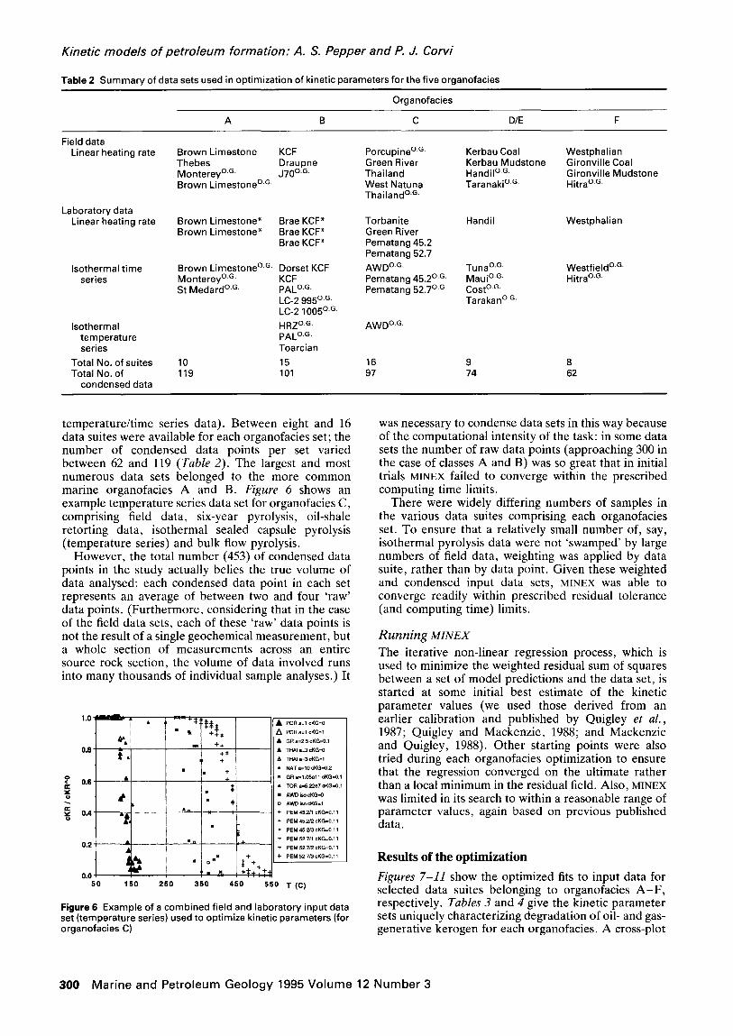
Table 2 Summary of data sets used in optimization of kinetic parameters for the five organofacies
Field data Linear heating rate
Laboratory data Linear heating rate
Isothermal time series
Isothermal temperature series
Total No. of suites Total No. of
condensed data
Organofacies
A B C DIE F
Brown Limestone KCF Porcupine”.G. Kerbau Coal Westphalian Thebes Draupne Green River Kerbau Mudstone Gironville Coal Monterey”.G. J70°.G. Thailand Handil”.G. Gironville Mudstone Brown Limestone”.G. West Natuna Taranakioo Hitra”-G.
Thailand”.G.
Brown Limestone* Brae KCF* Brown Limestone* Brae KCF*
Brae KCF*
Brown Limestone”.G. Dorset KCF Monterey”.G. KCF St Medard”.G. PAL”.G.
LC-2 995o.e. LC-2 1005o.o.
HRZ”.G. PAL”.G. Toarcian
Torbanite Handil Westphalian Green River Pematang 45.2 Pematang 52.7
AWD”.G. Tuna”.G. Westfield”.G. Pematang 45.2°.G. Maui”.G. Hitra”.G. Pematang 52.70c c0sto.e.
Tarakan”.G.
AWDoe
10 15 16 9 8 119 101 97 74 62
temperature/time series data). Between eight and 16 data suites were available for each organofacies set; the number of condensed data points per set varied between 62 and 119 (Table 2). The largest and most numerous data sets belonged to the more common marine organofacies A and B. Figure 6 shows an example temperature series data set for organofacies C, comprising field data, six-year pyrolysis, oil-shale retorting data, isothermal sealed capsule pyrolysis (temperature series) and bulk flow pyrolysis.
However, the total number (453) of condensed data points in the study actually belies the true volume of data analysed: each condensed data point in each set represents an average of between two and four ‘raw’ data points. (Furthermore, considering that in the case of the field data sets, each of these ‘raw’ data points is not the result of a single geochemical measurement, but a whole section of measurements across an entire source rock section, the volume of data involved runs into many thousands of individual sample analyses.) It
T W
Figure 6 Example of a combined field and laboratory input data set (temperature series) used to optimize kinetic parameters (for organofacies C)
was necessary to condense data sets in this way because of the computational intensity of the task: in some data sets the number of raw data points (approaching 300 in the case of classes A and B) was so great that in initial trials MINEX failed to converge within the prescribed computing time limits.
There were widely differing numbers of samples in the various data suites comprising each organofacies set. To ensure that a relatively small number of, say, isothermal pyrolysis data were not ‘swamped’ by large numbers of field data, weighting was applied by data suite, rather than by data point. Given these weighted and condensed input data sets, MINEX was able to converge readily within prescribed residual tolerance (and computing time) limits.
Running MINEX The iterative non-linear regression process, which is used to minimize the weighted residual sum of squares between a set of model predictions and the data set, is started at some initial best estimate of the kinetic parameter values (we used those derived from an earlier calibration and published by Quigley et al., 1987; Quigley and Mackenzie, 1988; and Mackenzie and Quigley, 1988). Other starting points were also tried during each organofacies optimization to ensure that the regression converged on the ultimate rather than a local minimum in the residual field. Also, MINEX was limited in its search to within a reasonable range of parameter values, again based on previous published data.
Results of the optimization Figures 7-11 show the optimized fits to input data for selected data suites belonging to organofacies A-F, respectively. Tables 3 and 4 give the kinetic parameter sets uniquely characterizing degradation of oil- and gas- generative kerogen for each organofacies. A cross-plot
300 Marine and Petroleum Geology 1995 Volume 12 Number 3

Kinetic models of petroleum formation: A. S. Pepper and P. J. Cot-vi
1.0
0.8
;5 0.6
z
8 0.4
0.2
(a)
BROWN LMSTOE 10
0.6
Figure 7 Selected examples of the input data and results of kinetic optimization for organofacies A. (a) Naturally heated Monterey Formation samples, onshore California; C&$I? ks = 0; heating rate 12XC Ma-‘; new proprietary data. Also plotted: laboratory bulk flow pyrolysis of two Brown Limestone Formation samples, Gulf of Suez; C & /C & = 0.29; heating rate 25°C min’; old proprietary data. (b) Laboratory sealed capsule pyrolysis of an Upper Jurassic sample from the Aquitaine Basin, France; C&/C& = 0; isothermal at 370°C; new proprietary data
.\. 100 200 300 400
TEMPERATURE (CENTIGRADE)
of A versus E,,,, (fully independent variables in the optimization) for all the results (Figure 12) shows that they co-vary in the general manner observed for other geochemical reactions (Wood, 1988). Before applying the results, however, we checked our confidence level for each parameter set.
Oil generation parameters The oil-generative kerogen results (Table 3) appear robust. Initially we were concerned that the small oE value for organofacies C kerogen might simply reflect a relatively small number of samples with less geological scatter (Figure 6). However, as organofacies D/E and F data sets had fewer data suites, but produced a larger optimized on, we believe that the relatively tight activation energy distribution of organofacies C is not an artifact of this sort.
Gas generation parameters Results for the gas-generative kerogens (Table 4) must carry less confidence than those for oil-generative kerogen, if only because of their relative concentrations
Table3 Results of optimization of kinetic parameters for oil generation from the five kerogen organofacies
Organofacies (Al,
E mean (SE (kJ mol-‘1 (kJ mol-‘1
A 2.13e13 206.4 8.2 B 8.14eT3 215.2 8.3 C 2.44e’4 221.4 3.9 DE 4.97e’4 228.2 7.9 F 1.23e” 259.1 6.6
UN
STMEDARO
(Figure 2). Thus, gas-generation data are more ‘noisy’, being more susceptible to measurement errors and the effect of natural scatter. We have particularly low confidence in the organofacies D/E gas-generative parameters and believe that the very low A and E,,,,, values are in this instance a spurious result based on a poor data set; we recommend that the kinetic data for gas-generative organofacies F is used instead (see later for discussion). There is a fairly wide variation within the remaining gas-generation parameters, the most reliable being organofacies F, which typically have relatively gas-rich reactive kerogens (relatively low HI” and high G”; Figure 2).
As organofacies A, B, C and, to a lesser degree, D/E, typically have gas-poor reactive kerogens (rela- tively high HI” and low G”; Figure 2), the overall effect of any errors in the kinetic description of gas generation on the bulk generation profile will be small (see later). Furthermore, Parts II and III will show that gas yields directly from kerogen are not the prime causes of gas- proneness in source rocks.
Table4 Results of optimization of kinetic parameters for gas generation from the five kerogen organofacies
Organofacies
A 3.93e12 206.7 10.7 B 2.17e’* 278.7 18.4 C 2.29e16 250.4 10.1 DE* 1.88e” 206.4 7.7 F 1 .93e16 275.0 9.9
*Considered unreliable and unrealistic - instead use F
Marine and Petroleum Geology 1995 Volume 12 Number 3 301

Kinetic models of petroleum formation: A. S. Pepper and P. J. Corvi
= 0.6
E
i 0.4
0.8
570, UK CNS KCF, RRAE TOARCIAN
(a)
TEMPERATURE (CENTIGRADE)
0 I
0.8
Z 0.6
i
H 8 0.4
1.0
0.8
0.2
l-
-r
(b)
---I d
l&J 2&l 360 4io vi3 TEMPERATURE (CENTIGRADE)
LC-2,1005
2am5mw75arJlmmlwmlsaxa175omnrmo2mao TIME BECGNDS)
Figure 8 Selected examples of the input data and results of kinetic optimization for organofacies B. (a) Naturally heated samples from the ‘J70’ Upper Jurassic Kimmeridge Clay Formation ‘hot shales’, UK North Sea; Co /Co ke kR = 0.18; heating rate = 1°C Ma-‘; new proprietary data. Also plotted: laboratory bulk flow pyrolysis of three samples from the Upper Jurassic Kimmeridge Clay Formation, Brae area, UK North Sea Basin; Co /Co - xo kR - 0.18; heating rate 25°C min’; sample of Toarcian mudstone, Paris Basin; Co /Co
old proprietary data. (b) Laboratory hydrous pyrolysis of a ke kR = 0.15; isothermal heating for 48 hours at differing temperatures; data from
Bertrand et a/. (1987). (c) Laboratory sealed capsule pyrolysis (SCP) of a sample of Liassic mudstone, Germany; C&&&r = 0; isothermal heating for 72 hours at differing temperatures; old proprietary data. (d) Laboratory SCP of a sample of Carboniferous mudstone, East Midlands, onshore UK; C&& :a = 0; isothermal heating at 370°C; new proprietary data
302 Marine and Petroleum Geology 1995 Volume 12 Number 3

Kinetic models of petroleum formation: A. S. Pepper and P. J. Corvi
$ 0.6
F d
5
!! 8 0.4
TEMPERATURE W2ENTffiRADE)
1.0 GREEN RIVER
0.8
2 1 0.6
h 8 0.4
02
(a)
l&l 2&J 3&l 4&l Sk
TEMPERATURE (CENTIGRADE)
(6
1.0
0.6
Z 0.6 0 F
f
8 0.4
0.2
(b)
AWO
b
d
f
l&I A0 3bo 4&l
,EMPERATURE V2ENTlGRADE~ 5bo
PEM 52.7
WI Figure 9 Selected examples of the input data and results of kinetic optimization for organofacies C. (a) Naturally heated samples from Oligocene mudstones, Natuna Sea, Indonesia; C’&/C & = 0.20; heating rate 7.5”C Ma-‘; new proprietary data. Also plotted: three repeats of laboratory bulk flow pyrolysis of a Palaeogene Pematang Brown Shale sample, Central Sumatra, Indonesia; C”,c/C”,, = 0.11; heating rate 33.2”C min-’ (Figure 4); new proprietary data. (b) Laboratory sealed capsule pyrolysis (SCP) of a Bathonian oil shale sample, Scotland; C& = 0; isothermal heating for 72 hours at differing temperatures; proprietary data. (c) Thermal solution of a sample of Green River Formation mudstone; C ‘& /C ‘& = 0.10; heating rate 02°C min-‘; new data from Leavitt et al. (1987). (d) Three repeats of laboratory SCP of a Palaeogene Pematang Brown Shale sample, Central Sumatra, Indonesia; C&/C& = 0; isothermal heating at 370°C; new proprietary data
Marine and Petroleum Geology 1995 Volume 12 Number 3 303

Kinetic models of petroleum formation: A. S. Pepper and P. J. Corvi
1.0
0.8
ii O6 z’
B U 0.4
0.2
(a)
KAPW
I . . . . I
100 200 300 400 500 TEMPERATURE (CENTIGRAM)
100 2&J 360 4&l 5iJO TEMPERATURE (CENTIGRADE)
(cl
1.0
0.8
z 0.6
E z
I 0.4
0.2
1.0
0.8
g 0.6
d 5
H 8 0.4
0.2
(b)
KERBAU MUDSTONES
I 1 , 1 I
100 200 300 400 500 TEMPERATURE KZENTIGRADE)
I
ii
.
.
msoax,7mlomool25amlsom,l7som2amomoa, TIME (SECONDS)
(d)
Figure 10 Selected examples of the input data and results of kinetic optimization for organofacies D/E. (a) Naturally heated coal samples from the Palaeogene Kapuni Formation, Taranaki Basin, New Zealand; C&/C& = 0; heating rate 2°C Ma-‘; new proprietary data. (b) Naturally heated Miocene mudstone samples from the Balikpapan Formation, Kerbau well, Kutei Basin; C”,&“,, = 0.21; heating rate 7.5”C Ma-‘; new data from Hut er al. (19871, Durand et al. (1987) and others. (c) Naturally heated Miocene coal samples from the Balikpapan Formation, Handil field, Kutei Basin; C’&/C? kR = 0; heating rate 7.5”C Ma-‘; new data from Ungerer eta/. (1986). n.._...._l _* ^I ,.ln0-J\ ^._..I ̂ .k^_^ A,^^ ..,-+*-.-I. I^~^_..+ ̂ ..., k..ICII ^._, ^.._ ..I..^:^ -c ^ ^^^I -..-_I- ‘--- &k^ -^-^ ^^.._^^. PO IPO - n ,c. U”,dl,” rx a,. , ,JO,, a,,” “LIIcilh r\lD” p,l”Lrr;“. lau”,aLury KJUIF. ll”W )Jy1v,ys,a “I a L”al aa,,,p,e ll”lll Lllci 3Qllle DVUILC, bK(ybKR - “. I”, heating rate 25°C Ma-‘; data from Ungerer et al. (1986). (d) Laboratory sealed capsule pyrolysis of a sample of Palaeogene coal, Gippsland Basin, offshore Australia; C EG /C zR = 0; isothermal heating at 370°C; proprietary data
304 Marine and Petroleum Geology 1995 Volume 12 Number 3

10
0.6
2 P 0.6
d 5 g s 0.4
02
10
08
z E 0.6
5
8 * 0.4
02
(a)
Kinetic models of petroleum formation: A. S. Pepper and P. J. Corvi
L--- 100 2oc 300 400 500 l&l 260 3bo 460 560
TEMPERATURE (CENTIGRADE) TEMPERATURE (CENTIGRADE)
(cl (d)
10
0.8
z 0.6 0 F 2
t,., 0
02
1.0
0.8
5 06
1
1 04
0.2
(W
WESTPMLIAN COAL
-A \
wEsTFlElD
Figure 11 Selected examples of the input data and results of kinetic optimization for organofacies F. (a) Naturally heated coal samples from the Hitra Formation, Haltenbanken, offshore Norway; C? /Co - kG kR - 0, heating rate 4.5”C Ma- ‘; new proprietary data. (b) Laboratory bulk flow pyrolysis of a sample of Westphalian coal from onshore UK; C EG /C & = 0.35; heating rate 25°C Ma-‘; old proprietary data. (c) Laboratory sealed capsule pyrolysis of a Hitra Formation coal, Haltenbanken, offshore Norway; C&/C”,, = 0; isothermal heating at 370°C; old proprietary data. (d) Laboratory sealed capsule pyrolysis of a sample of Namurian vitrinitic coal, Westfield mine, Scotland; C&/C& = 1; isothermal heating at 370°C; old proprietary data
Marine and Petroleum Geology 1995 Volume 12 Number 3 305

180 200 220 240 260 280 300
Emean (kJ mol*-1)
Figure 12 Relationship between optimized A versus E,,,,,, for the five organofacies. Symbols surrounded by large circles denote gas-generative fractions; uncircled symbols denote oil- generative fractions
Links between kinetic parameters and organic precursor chemistry
There remain few simple, unambiguous links between the kerogen breakdown kinetics and the chemistry and structure of the precursor kerogen; some of those which have been proposed remain the subject of debate. This reflects the difficulties inherent in under- standing a substance which, by definition, is insoluble in most common solvents and to date has been studied largely by means of degradative (pyrolysis) or oxidative techniques. We cannot pretend to understand in detail the fundamental chemical controls governing our kinetics parameter sets, and present the following observations as discussion points only.
Orr (1986) and Baskin and Peters (1992) suggested that the known weak strength of carbon-sulphur bonding is the direct cause of relatively early break- down of high sulphur kerogens, such as the Monterey Formation of California. Orr (1986) proposed a new kerogen classification: type IIS, defined as a kerogen containing in excess of 8 wt.% sulphur. Hunt et al. (1991) noted an inverse relationship between sulphur content and activation energy in a series of type II kerogens. Tannenbaum and Aizenshtat (1985) argued that high concentrations of heteroatoms other than sulphur (i.e. N, 0) may also influence the kinetics of generation in the Senonian bituminous chalks of the Dead Sea Graben, Israel.
The Monterey and other high sulphur kerogens conform to our organofacies A (Table I), which posses- ses the lowest E,,,, for both oil and gas generation of all the organofacies (Tables 3 and 4). Tissot et al. (1987) also showed examples of carbonate-rich source rocks with low (laboratory-derived) activation energies.
Although these are valid observations, a global causal relationship between organic sulphur content and activation energy remains unproved. Figure 13 appears to show a crude systematic decrease in E,,,, with increasing S/C ratio for the oil-generative portions of organofacies A-F kerogens. However, as shown in isothermal pyrolysis experiments by Bar et al. (1988a; 1988b), a simple causal link between gross sulphur
Kinetic models of petroleum formation: A. S. Pepper and P. J. Corvi
content and kerogen activation energy may be an over- simplification: the structural position of the sulphur in the kerogen may be more important.
The boundary between organofacies B and A is necessarily ‘fuzzy’ because of the natural gradation between clay- and carbonate-rich mudstones. Here, lithology is more important than organic input (Table I). In contrast, activation energy distributions for organofacies B and C (types II and I, respectively) differ because of organic input (?and possibly pore- water sulphate content/sulphur incorporation). Type I kerogens have a narrow range of bond strengths arising from the dominance of cross-linked aliphatic chains, where strong C-C bonds predominate (Tissot et al., 1987; Bar et al., 1988a; Sundararaman, 1988). This situation is typical of kerogens rich in the remains of freshwater algae, which synthesize long unbranched alkane chains (waxes) as a buoyancy aid. Our results for organofacies C, which has the tightest distribution of energies (lowest on) are consistent with this idea.
There have been various claims and counter-claims about the potential role of resinite in petroleum generation, particularly at very low levels of thermal stress (Snowdon and Powell, 1982; Mukhopadhyay and Gormly, 1984; Lewan and Williams, 1987; Powell and Boreham, 1994). However, access to reliable data sets at the time of study prevented us from investigating separately the generation behaviours of organofacies D (wax-rich) versus E (wax-rich plus resin-rich).
The higher E,,,, of oil-generative F relative to D/E may result from greater lignin content and an increas- ingly aromatic kerogen structure and, conversely, relative enrichment of D/E in cuticular waxes (and/or resin and/or bacterial lipids). Note a wax-lignin mix would be consistent with an E,,,, (228.2 kJ mol-‘) for D/E intermediate between that of wax-rich C (221.4 kJ mol-‘) and lignin-rich F (259.1 kJ mol-‘).
0
Figure 13 Possible role of sulphur in determining activation energy of oil generation reactions. Sulphur to carbon ratios for some rocks belonging to organofacies A-F are derived from a compilation of proprietary and published data (courtesy of Dr A. Aplin; note that these S/C data were not derived for the exact samples- or in some cases even the same source rock suites- used to calibrate the kinetic parameters for each organofacies). Boxes define fl standard deviation in (SIC) kerogen and activation energy
306 Marine and Petroleum Geology 1995 Volume 12 Number 3

Lignin-rich organofacies F may be represented petrographically by the vitrinite maceral, whose structure is one of the aromatic rings cross-linked by short (up to C,) aliphatic chains - a thermally robust configuration (Quigley et al., 1987). Both gas and aromatic oil (‘coal tar’) are likely to be liberated on disintegration of the same bonds in the macro- structure. In this context it is interesting to note the similar E,,,, obtained for oil and gas generation from organofacies F. Our decision to adopt organofacies F gas generation parameters in place of those probably spurious results for organofacies D/E (Table 4) is supported by the likelihood that most gas from organofacies D, E and F kerogens originates from the same lignin-vitrinite precursor.
Synthetic compounds as analogues Additional information can be gleaned from the degradation of representative synthetic analogues, which are simpler than natural kerogens and provide a clearer insight into the underlying chemical and struc- tural mechanisms.
Bar et al. (1988b) found great similarity between the pyrolysis behaviour of a sample of Australian torbanite (freshwater algal coal: our organofacies C) and linear chain synthetic polymers, which allowed them to make inferences about the mechanism of degradation of the torbanite. Interestingly, their value for the activation energy of the inferred random depolymerization reaction (bulk reaction 236 k.J mol-‘) is intermediate
200 403 600
l!SOl-HERMAL TEMPERATURE PC)
Kinetic models of petroleum formation: A. S. Pepper and P. J. Corvi
between our organofacies C oil- (221.4 kJ mall’) and gas-generative (250.4 kJ mol-‘) component values, and hence consistent with a mixture of the two.
Synthetic lignins could be regarded as chemical and structural analogues to vitrinitic organofacies F. Avni et al. (1985) subjected lotech lignin to 80 s flash pyrolysis at various temperatures, deriving kinetic parameters describing the production of various species including methane and tar. Figure 14 compares our predictions (using our kinetic parameters for degradation of oil- generative organofacies F; Table 3) with their observa- tions of tar evolution; the test lies well outside the range of thermal regimes used in our calibration. The kinetic model of Avni et al. (1985) is also shown, but note that their model was fitted to these data. At best, there is only general agreement between our prediction and the observations, suggesting that the results of such studies need careful interpretation. As shown by Stout et al. (1988), many chemical changes occur as lignin becomes transformed during early diagenesis into the maceral vitrinite. These transformations may alter the resulting composition and structure sufficiently that the analogy between supposed precursor and actual sub- surface reactant becomes strained.
Application of the kinetic model in exploration
Now we turn away from theory and towards our most important objective: application of the kinetic model in petroleum exploration.
Kerogen degradation projiles The most graphic way to visualize the effects of differences in kinetic parameters is to construct a comparative series of kerogen degradation profiles, initially at a common, simple linear heating rate. We choose 2°C Ma-‘, which is in our experience close to a global average for many basins currently in the post-rift stage of thermo-tectonic evolution. Our convention is to denote the heating rate by a subscript, i.e. in this instance we will use a subscript 2, e.g. OGTz refers to the OGT reached at a heating rate of 2°C Ma-‘. The actual effect of heating rate will be discussed later.
Reactive kerogens are never pure end-members of oil-generative or gas-generative kerogen: they are mixtures. As we have determined separately the kinetics of the two end-members for each organofacies A-F, we can construct kerogen degradation profiles by recombining oil- and gas-generative kerogens in any desired proportion (Figure 1.5). The progressive inclusion of greater (higher activation energy) gas- generative proportions in the reactive kerogen mix tends to produce elongate ‘tails’ of increasing size in the high-temperature portions of a degradation profile.
Dejinition of ‘oil and gas windows’
Figure 14 Model compounds as potential analogues in the study of petroleum generation: comparison of tar evolution during laboratory pyrolysis of a synthetic lignin (Avni et a/., 1985) with predictions based on oil-generative organofacies F kinetic parameters
Before showing the impact of our work in delimiting petroleum generation zones in the geological sub- surface, we wish to clarify a point which in our experience has caused confusion amongst petroleum explorationists working with concepts such as ‘oil generation threshold’: actually there is no theoretical basis for a threshold of any sort. The Arrhenius equation [Equation (12)] dictates that the reaction rate k will never be zero as, until the temperature drops to
Marine and Petroleum Geology 1995 Volume 12 Number 3 307
Kinetic models of petroleum formation: A. S. Pepper and P. J. Cot-vi
Organofacies A Organofacies F
70 100 130 160 190 220 250 70 100 130 160 190 220 260
0rganofacies B 1) Oil-generative kerogen
70 100 130 160 190 220 250 4
70 100 130 160 190 220 260 T (C) at 2 C/Ma
Organofacles c g) Gasgenerative kerogen
70 100 130 160 160 220 260 70 100 130 160 190 220 260
T (C) at 2 C/Ma T(C) a, 2 c/Ma
Organofacies DIE
70 100 130 160 190 220 260 T(C) at 2 C/Ma
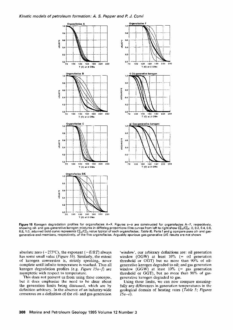
Figure 15 Kerogen degradation profiles for organofacies A-F. Figures a-e are constructed for organofacies A-F, respectively, showing oil- and gas-generative kerogen mixtures in differing proportions (line curves from left to right show CEe/C&: 0,0.2,0.4,0.6, 0.8, 1 .O; adorned bold curve represents C&/C& value typical of each organofacies; Table 6). Parts f and g compare pure oil- and gas- generative end-members, respectively, of the five crganofacies. Arguably spurious gas-generative D/E results are not shown
absolute zero (-273”C), the exponent (-EIRT) always has some small value (Figure 16). Similarly, the extent of kerogen conversion is, strictly speaking, never complete until infinite temperature is reached. Thus all kerogen degradation profiles (e.g. Figure 1.5a-J) are asymptotic with respect to temperature.
This does not prevent us from using these concepts, but it does emphasize the need to be clear about the generation limits being discussed, which are by definition arbitrary. In the absence of an industry-wide consensus on a definition of the oil- and gas-generation
‘window’, our arbitrary definitions are: oil generation window (OGW) at least 10% (= oil generation threshold or OGT) but no more than 90% of oil- generative kerogen degraded to oil; and gas generation window (GGW) at least 10% (= gas generation threshold or GGT), but no more than 90% of gas- generative kerogen degraded to gas.
Using these limits, we can now compare meaning- fully any differences in generation temperatures in the geological domain of heating rates (Table 5; Figures 152-e).
308 Marine and Petroleum Geology 1995 Volume 12 Number 3

60E & laquJnN ZL awn[o~ 5661 ABo[oag uJna[o.i~ad pue auyeyy
(9LL = u) .IH 601 61’0 - ZL’O = :oD b’) P”e f(L46 = U) JH 601 61’0 - OL’O = .E) (E) :(LPL = u) .IH 601 91‘0 - Z9’0 = .E) (Z)
:(,ld - l)/(,lH . old) = .I1 It) :=h-ww’w~ =!K’!PaJd (01s + .tSVotS = old !wsAlo~Ad oZS lW’U(‘-L3J3
= ok !JOJ.&ZS + .LS) = XI !,30UoZS = AH :,30UoLS = .I1 :sJaa~e’ed
s~!wy y006-0~ asooy3 am ‘uo!ssnmp JnO up ‘lahal uo!)eJaua6 40 anleA AJeJl!qJe ai_uos 01 a3uaJa4aJ saAjohu! Al!Jessaaau saJnieJadu!az uo!]eJaua6 40 uo!ssnmp Aue a3uaH ‘OJaz JaAau s! aleJ aLj1 :wnnu!~uo3 e aq 0) uaas s! uojleJaua6 UInalOJIad ale% 3!urql!Je6ol e uo paMa!A uaqM gL aln6!j
t 1 VP’0 10’0 091 84 1 z 4 P 1 EZ’O ZO’O OPE EEE L 3/a & 1 El’0 EO’O oz9 009 oz 3 E 1 Lt.0 EO’O 019 Z69 81 8 Z 1 LL’O SO’0 099 L19 EE v
23 011 (L. 3 6 6uJ)
etep .IH “0 23 .Id XI .IH .I1 sa!3e4oue6Jo paseq sd!qsuo!lelaJ
aA!lNPaJd
wm z ae (3) I OS1 OZC 06 09
UMOUy S! ,$-j ttlll0 alaL+ SUO!l
-enl!s Jo4 sd!ysuoyelaJ ah!p!paJd pue sa!3e4oue6Jo aA!4 aq1 40 sJaqwaLu leD!dAl 40 scys!Ja13eJey lez+uaq3oa6 leyyl g alqal
arlyymm e u0 ‘3-V say~3oue%o ucqj samwadura$ .1aq8!y q3nw or? se8 .r!aql p[a!IC (uogepe.12ap ua8o.ray mold-se2 103 sra)aumed 3yaug sum aq~ paumsse a~eq 3~ asnmaq sa pm) d sa~~r23oueS~O .sa%js ~a]e[ aq$ u! 8uyoaa se8 alow l#M ‘a[yoId uo!w1aua8 aql u! /([.~a spnpoId 809 MO[ 103 s! kmapual aq~ (.lunst) slsnpold uoy~aua8 aa~~~[nruns aql u! se8 JO UO~X.IJ SSBW aq~ 01 sra3a.1 a.~aq uog!sodwo3) ‘081 a.&hg u! sape3oue~.10 [eg!diCl Amy sum aq$ lo3 soy21 [suog!soduroD pawaua8 30 uogn[oAa ayl iC[amadas SMOyS 481 aA?l&Q wmpold aq$ 30 uoysoduro3 %IIA[OA3 3q$ $3+JaJ 2-DLl S%ld%LJ UO St?‘CIl~ p![OS OM$
aql JO suoglodo.Id 3A!]E[CX aq~ ‘[apotu aqj u! ICIluapuad -apI+ 3pW83p SU38Olay ~A!~Iz?.IXI3h28 PllF? -[IO SV
uoyelaua8 u.ma[oIlad 30 suogd!.map ala[dwom! am ~1 a.&?!d II! UMO~[S sahm3 ,[eD!dlCl, aq$ uaAg
sapJoAd uoyvnauag
qXa .I03 ]QH 30 UO!Ul[OAa aql SMOqS D8781%4?‘?8~~ ‘(8861)
iCa[Z!n~ put3 a!zuayxl/y nsuas (Igd) xapu~ uoy2aua8 wna[ollad pue (9861) ‘10 la ~a[003 nsuas (IgE)H) xapu! uoyx~1a8 uoqlmolpdq sapyuenb aql 01 spuodsallo3 amaq pue - pa~waua8 uaaq seq q3!qM [gualod [egy 30 uoym3 a~ye[num [UOJ aql swasaldal sea.~ se% sn[d [!o pawqmo3 aql30 punoq laddn aql Jeql 3JON .ssa.~~s [“umq$ %I~sE?~.I~I! 01 asuodsal ur saper8ap uaBo_~ay se smpo.Id uo~~wauaB aAgeInum3 aql JO uoge.wamo~ 8u@ueq3 aq$ Moqs sa[yold uoyauaf)
(i a[yold aql30 u1.103 aql 01 8ugnqnwo3 am sluauoduro:, ua8olay OMJ sn[d wauodwo3 1’0 [ey!u! LIE? SE ‘dIIn3alm alow uaAa pay[mb aq wm.u (~90, 3.a) laAa[ uopkmwu 30 sluaurawis ‘araq leql aloN) .(2-r) L [ am&~) sa[yo.td uopwaua8 ,[mrdAl, pamwsuo3 amq aM ‘sa!2e3ou&o a,zy aql 103 ‘uoyeq I!0 [r?gu! aq$ BuIpnIm! awg s!ql ‘suoysodtuo3 %y.w~s amwmu! [eD!diCl aApap 01 9 alqvL %u!sn ‘urei?V ‘(I am8y) uoy3ey [lo [eyu! ue 103 iunome $0~ op hayi asnwaq
30 aAy?$uasa~dal sa[dum 30 laqumu a&?[ 1! .103 elep IwyaqDoa8 Bu!Be~aAe /cq pa+ap amM s.Ia)aumed iIne3ap asaqL ‘9 alqvJ uro.13 uayel alam sl a.W%g uo ua2iolay aywaua%seil pm [IO 30 suoyewamo~ [eyu! [myddl ‘a[dmexa KJ+J ‘9 alqvJ uo paz+wmms a.re sayadold [ey.uaq~oail [egyr asoqm say3oue8ro qDea JO slaqumu ,[rm!dlCt, @sn (111 pm [I wed LI! asoql ??u!pn[m) [apow 3pau!y mo JO si[nsal aql JO hm aywsn[[! [[IM aM ‘JaliaMoH .sa.wx!ru u&?o_tay sno!.m ~03 sa[yold uhiopyealq ua8olay sMoqs I;[ aAn8y
ozz ozz OLL otz 991 aseg
(w) ‘XL (w) 9Lt (‘GE) SE1 (OL) 081 (09) 901 (a6ueJ) do1 (30) MoPu!M se!3
4LL 091 OPL 4PL SEL asea
(OE) 9Pl (OP) OZL (01) OZL (OP) 901 (OP) 96 (a6ueJ) do1 (30) MoPu!M I!0
3 3/a 3 8 v
sa!Se4oue6J()
,-ew 3.2 = aleJ 6u!,eaq amaJa4aJ :Si3!3e$OUe6JO aA!4 aq, Jo4 (suo!ly!4ap JO4 lxal aas) SMOPU!M se6 pue l!o aq$40 sy_u!l aJnleJadura1 g alqel
sa@aua uoyilye 30 a8uel .c3[[etus c ~013 slInsala12.m 3 sape3oue%o aq$ 30 adoIs ladaays ~Iwm~u8~s aql f sa~.m uogepw%ap ua%!olay aql u! sado[s x[~.I.I~s asnw (,g alqvL) d pm ga ‘8 ‘v sa!~r?Jout&o ~013 uogmaua8 I!0 103 30 30 san[m .n+u!s iC[peolq aql leql sMoqs os[e Jg a.W%y ‘(s alqvJ> g saoce3oue2ho 103 3,SLl -Spl w pur! V sa!m3om%~o 103 30Sc~-S6 ‘~3 uaaiM$aq say24 ‘M1;)O ‘(E alqvL> LI 01 V JaPJo aql u! ,_I(‘” l-7 6SZ ‘83 01 ~ _[ow fy 9oZ ‘~3 u1013 Ueawg u! aseamy Impw2 e A‘I lno‘lc lq8noJ‘l s! lJ!qS s!q.L ‘(S alq?Z) 3,SPI ol S6 ‘W uIol3 d 01 V lap10 aq4 u! sawamu! 2~90 :(& am&J) iue~yyii?!s ale sape3ou&%o uaaMiaq samalag!a

Kinetic models of petroleum formation: A. S. Pepper and P. J. Corvi
a) Typical A d) Typical DE
_.- 70 100 130 160 190 220 250 70 100 130 160 190 220 250
T (C) at 2CIMa T (C) at 2 C/Ma
b) TYPiCal B e) Typical F
70 100 130 160 190 220 250 70 100 130 160 190 220 250
T (C) at 2 C/Ma T (C) at 2 C/Ma
c) Typical C 1.0 , I I 1
-70 100 130 160 190 220 250
T (C) at 2 C/Ma
Figure 17 Generation profiles for typical members of organofacies A-F, shown on parts a-e, respectively. HGI curves for these typical members are compared in Figure 18a
basis, the product composition is strongly oil- dominated, as dictated by the input values of Go (Figures 2 and 3; Table 6). Even in the case of organofacies F, G,,, only exceeds 0.4 at very high thermal stress levels (T2 ca. 220°C).
Generation profiles are illustrative, but are not helpful in predicting the actual petroleum charge from a source rock; they represent only the first building block in a full description of petroleum formation. This is because Figures 17 and 18 represent a geologically trivial case: a fully open system, where all products are immediately expelled before oil cracking can take place. Although this may sound obvious, we are continually surprised to read modern exploration case histories where the geochemical evaluation stops at precisely this level of evaluation of the source kitchen.
Effect of time
Heating rate So far we have confined ourselves to discussing differ- ences in generation behaviour at a reference heating rate (2°C Ma-‘). In Figure 19 we examine the effect of different heating rates on the temperatures at which petroleum-generating reactions occur. As an illustra- tion, we consider only the lowest and highest activation energy species: oil-generative organofacies A and gas- generative F. The range of heating rates (0.5-50X Ma-‘) encompasses the extremes encountered in sedimentary basins unaffected by igneous intrusions. For example, heating rates on old passively subsiding continental margins or in old intra-continental basins may be 1°C Ma-’ or lower (e.g. Scotian Shelf; Paris
310 Marine and Petroleum Geology 1995 Volume 12 Number 3
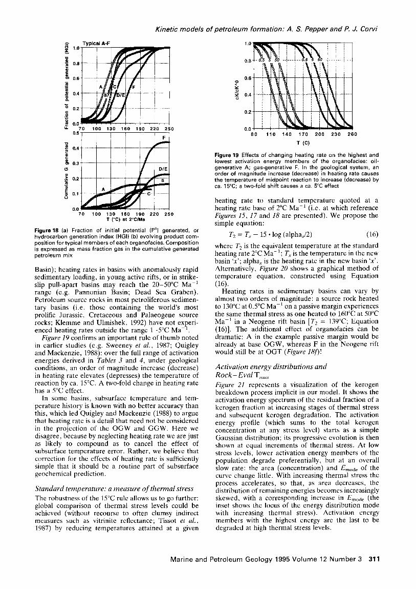
Kinetic models of petroleum formation: A. S. Pepper and P. J. Corvi
n g 0.8
t g 0.6 3 E d 0.4 x
100 130 160 190 220 250 /
-70 100 130 160 190 220 250 T ("C) at 2WMa
Figure 18 (a) Fraction of initial potential (PO) generated, or hydrocarbon generation index (HGI) (b) evolving product com- position for typical members of each organofacies. Composition is expressed as mass fraction gas in the cumulative generated petroleum mix
Basin); heating rates in basins with anomalously rapid sedimentary loading, in young active rifts, or in strike- slip pull-apart basins may reach the 20-50°C Ma-’ range (e.g. Pannonian Basin; Dead Sea Graben). Petroleum source rocks in most petroliferous sedimen- tary basins (i.e. those containing the world’s most prolific Jurassic, Cretaceous and Palaeogene source rocks; Klemme and Ulmishek, 1992) have not ex
I: eri-
enced heating rates outside the range l--SC Ma- . Figure 19 confirms an important rule of thumb noted
in earlier studies (e.g. Sweeney et al., 1987; Quigley and Mackenzie, 1988): over the full range of activation energies derived in Tables 3 and 4, under geological conditions, an order of magnitude increase (decrease) in heating rate elevates (depresses) the temperature of reaction by ca. 15°C. A two-fold change in heating rate has a 5°C effect.
In some basins, subsurface temperature and tem- perature history is known with no better accuracy than this, which led Quigley and Mackenzie (1988) to argue that heating rate is a detail that need not be considered in the projection of the OGW and GGW. Here we disagree, because by neglecting heating rate we are just as likely to compound as to cancel the effect of subsurface temperature error. Rather, we believe that correction for the effects of heating rate is sufficiently simple that it should be a routine part of subsurface geochemical prediction.
Standard temperature: a measure of thermal stress The robustness of the 15°C rule allows us to go further: global comparison of thermal stress levels could be achieved (without recourse to often clumsy indirect measures such as vitrinite reflectance; Tissot et al., 1987) by reducing temperatures attained at a given
0.6
s g 0.4
80 110 140 170 200 230 260
T (C)
Figure 19 Effects of changing heating rate on the highest and lowest activation energy members of the organofacies: oil- generative A; gas-generative F. In the geological system, an order of magnitude increase (decrease) in heating rate causes the temperature of midpoint reaction to increase (decrease) by ca. 15°C; a two-fold shift causes a ca. 5°C effect
heating rate to standard temperature quoted at a heating rate base of 2°C Ma-’ (i.e. at which reference Figures 1.5, 17 and 18 are presented). We propose the simple equation:
T2 = T, - 15 ?? log (alpha,/2) (16)
where T2 is the equivalent temperature at the standard heating rate 2°C Ma-‘; TX is the temperature in the new basin ‘x7; alpha, is the heating rate in the new basin ‘x’. Alternatively, Figure 20 shows a graphical method of temperature equation, constructed using Equation (16).
Heating rates in sedimentary basins can vary by almost two orders of magnitude: a source rock heated to 130°C at 0.5”C Ma-’ on a passive margin experiences the same thermal stress as one heated to 160°C at 50°C Ma-’ in a Neogene rift basin [T2 = 139°C; Equation (16)]. The additional effect of organofacies can be dramatic: A in the example passive margin would be already at base OGW, whereas F in the Neogene rift would still be at OGT (Figure 18fl!
Activation energy distributions and Rock- Eva1 T,,, Figure 21 represents a visualization of the kerogen breakdown process implicit in our model. It shows the activation energy spectrum of the residual fraction of a kerogen fraction at increasing stages of thermal stress and subsequent kerogen degradation. The activation energy profile (which sums to the total kerogen concentration at any stress level) starts as a simple Gaussian distribution; its progressive evolution is then shown at equal increments of thermal stress. At low stress levels, lower activation energy members of the population degrade preferentially, but at an overall slow rate: the area (concentration) and Emode of the curve change little. With increasing thermal stress the process accelerates, so that, as area decreases, the distribution of remaining energies becomes increasingly skewed. with a corresponding increase in Emode (the inset shows the locus of the energy distribution mode with increasing thermal stress). Activation energy members with-the highest energy are the last to bk degraded at high thermal stress levels.
Marine and Petroleum Geology 1995 Volume 12 Number 3 311

Kinetic models of petroleum formation: A. S. Pepper and P. J. Corvi
25
-20 .I 1 10 100
Heating rate (C) Ma
Figure 20 Chart to correct temperature attained at any given heating rate to thermal stress comparator T2, i.e the equivalent temperature at a heating rate of 2°C Ma-‘. Add the correction factor appropriate for the basin heating rate to the actual temperature to arrive at the T2 equivalent (i.e. the reference at which Figures 75, 16 and 18 were constructed)
One of the major shortcomings of early single activation energy models was their inability to account for this shift in the residual activation energy, which is widely observed in experiments. Furthermore, given a standard heating rate regime such as Rock-Eva1 pyrolysis, Emode and T,,,,, (temperature of the maximum rate of S2 evolution) are proportional. This forms the theoretical basis for the use of pyrolysis T,,, as a source type specific maturation index (EspitaliC et al. ) 1977).
Testing the results of the kinetic model
Temperature prediction
To be truly universal, the kinetic parameters listed in Tables 3 and 4 must enable predictions to be made outside the range of data used to derive the kinetic parameters in the first instance. It is not sufficient to ‘test’ a model by comparing it with the data used to calibrate it in the first place! Some workers, projecting the results of laboratory pyrolysis to geological heating rates, have clearly been frustrated by a lack of access to field data, preventing these essential checks from being made (e.g. Burnham et al., 1987). Some attempts to fit field data have been frustrated by the geological
Figure 21 Changing activation energy distribution during kerogen breakdown, assuming an initial Gaussian activation energy distribution
312 Marine and Petroleum Geology 1995 Volume 12 Number 3
uncertainties inherent in understanding uplifted and eroded basins (e.g. Sweeney et al., 1987; Sweeney, 1988).In one published instance, where field data have been used to check laboratory-derived kinetic predic- tions (Ungerer et al., 1986; Ungerer and Pelet, 1987), a pragmatic result has been to change the kinetic para- meters, effectively resulting in a optimum fit based on both field and laboratory data (i.e. our approach).
We believe it is important to show fits to some of our input data so that readers can gain some feel for the natural variation in sample behaviour, potential errors in temperature estimation, etc. (Figures 7-11). However, the problem we encountered in attempting to find a ‘blind’ test of our kinetic parameters was that we had effectively exhausted all our best quality data sources in compiling the input data! Most remaining data sets were from basins where either geochemical or thermal data were sparse or unreliable. In some basins, vitrinite reflectance data rather than temperature were the main reference.
Figure 22, however, is an example of true ‘blind’ test of the model as the source rock and thermal regime considered were not included in the original calibra- tion. Data are derived from oil-shale retorting experi- ments (Leavitt et al., 1987) in which oil yields from the Sunbury Oil Shale, a marine organic-rich mudrock from the USA, are recorded with increasing tem- perature in experiments at two different heating rates. The sample is an algal/bacterial-dominated marine, siliciclastic-hosted kerogen, and therefore belongs to organofacies B (Table I). The curves show our model predictions for the appropriate heating rates. Clearly, there is excellent agreement between the kinetic model for the degradation of pure oil-generative organofacies B kerogen (using the parameters in Table 3) and this experimental data.
1.0
0.8
SLJNBURY OIL WALE
D.WC mid’ ??data - model
wdktii
3.!WC mii’ 0 data --- m&l
prediction
250 300 350 400 d
T (“C)
0
Figure 22 Testing the model: organofacies B oil-generative kerogen breakdown curves computed for heating rates shown, compared with experimental data from Sunbury Oil Shale (Leavitt et al., 1987)

Kinetic models of petroleum formation: A. S. Pepper and P. J. Corvi
Comparison with results of other models
Generally, we believe that inter-model comparison is a rather fruitless exercise, as the most important test of any model is how it compares with nature. However, a comparison is instructive in the light of earlier discus- sions in this paper about the validity and accuracy of extrapolating laboratory-derived kinetics to geological conditions. We compare our results with some from the IFP, i.e. Ungerer (1984), Ungerer et al., 1986), Ungerer and Pelet (1987), Tissot et al. (1987); from the LLNL (Lawrence Livermore National Laboratory), i.e. Burnham et al. (1987) and (1988); and from Sundararaman et al. (1988). This comparison is not exhaustive, but we believe a separate dedicated review would be timely and instructive.
Comparison of subsurfacepredictions
Both the IFP and LLNL schools, inter ah, propose that kerogen kinetic parameters can be characterized by laboratory pyrolysis of an individual immature sample, to reveal a unique, discrete distribution of activation energies. Tissot et al. (1987), amplifying the early work of Tissot and Espitalie (1975), however, recognize the common behaviour of global kerogen ‘types’ which bear some similarity to our organofacies A-F (Table I). Hence it is possible to begin to draw some comparisons between laboratory-derived sample- specific and combined field/laboratory-derived global kinetic parameters.
Figure 23 compares predicted bulk kerogen degrada- tion profiles using our kinetics for organofacies A, B, C and D/E and the approximate IFP equivalent types II‘S’JI, I and III‘H’, given a common thermal history: representing burial at 100 m Ma-r; surface tern
P era-
ture of 15°C; geothermal gradient of 33°C km- . On the left-hand side are the original IFP predictions (Tissot et al., 1987); on the right-hand side are our predictions for the equivalent organofacies.
Firstly, there are some differences which must be allowed for in the comparison. Firstly, the presented
IFP model predicts only bulk kerogen degradation. Because it does not differentiate oil and gas production from kerogen, we do not know the oil- and gas- generative proportions in the reactive kerogen; how- ever, using the published HI0 values for these samples, we estimate using Figure 2 that they are probably close to our ‘typical’ values (Table 6). This is unlikely to cause serious discrepancy between the two models. Secondly, behaviour derived from a large global data set in our model is compared against a number of ‘representative’ single samples. For example, type I behaviour is typified by an exceptionally hydrogen-rich sample of the Green River Shale (HI” = 898 mgHc gc-i); based on our review of lacustrine organofacies C (Table 6), this sample appears to be close to an end- member, and may be poorly representative of ‘lacus- trine’ kerogens in general.
There are both striking similarities and differences between the two sets of predictions. The relative order in which generation occurs with respect to temperature is the same for organofacies A, B and D/E (types II‘S’, II and III). All the curves are similar in general form, including the steep generation gradient calculated for both type I and organofacies C kerogens; in both cases the underlying cause is the tight distribution of bond energies (Table 3).
The most serious discrepancy is in the projected behaviour of the IFP type I and our organofacies C kerogen: the IFP model implies generation about 1 km deeper and 33°C hotter. This laboratory-derived kinetic behaviour has also been replicated by Sundararaman et al. (1988) for the Pematang Brown Shale, Indonesia and by Burnham et al. (1987) for an African type I sample (Figure 24 shows their activation energy distributions).
We currently lack a definitive explanation for this major difference but, given the global economic importance of lacustrine sourcing systems in Brazil, China, Indonesia (Katz, 1990) and other SE Asian areas, this problem deserves further study. In the meantime, two main factors persuade us that our model
1.0 0.0 0.2 0.4 0.6 0.8 1.0
Figure 23 Kinetic predictions for bulk kerogen breakdown, comparing typical members of organofacies A, B, C and D/E with possible representative IFP equivalent types II’S’ (Monterey Formation), II (Toarcian, Paris Basin), I (Green River Formation) and III’H’ (Handil Coal, Mahakam Delta) at a heating rate of 3.33”C Ma-’ (Tissot et al., 1987). The IFP predictions are laboratory pyrolysis-derived, except for the type Ill Handil coal. Legend follows Figures 75 and 18
Marine and Petroleum Geology 1995 Volume 12 Number 3 313
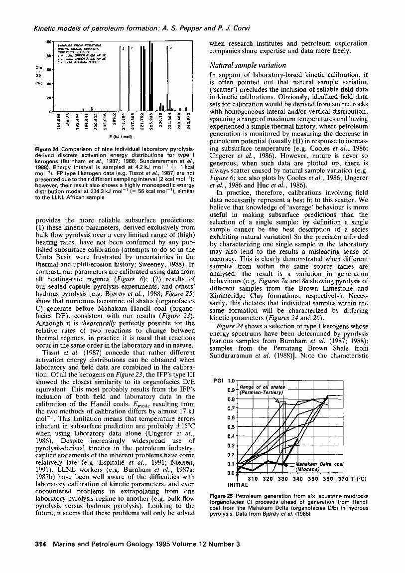
Kinetic models of petroleum formation: A. S. Pepper and P. J. Corvi
7-r 60-
X0
(%) 40-
E (kJ I mol)
kgure 24 Comparison of nine individual laboratory pyrolysis- derived discrete activation energy distributions for type I kerogens (Burnham et al., 1987; 1988; Sundararaman et al., 1988). Energy interval is sampled at 4.2 kJ mol-’ (= 1 kcal mol-‘). IFP type I kerogen data (e.g. Tissot et al., 1987) are not presented due to their different sampling interval (2 kcal mol-‘); however, their result also shows a highly monospecific energy distribution modal at 234.3 kJ mol-’ (= 56 kcal mol-‘), similar to the LLNL African sample
provides the more reliable subsurface predictions: (1) these kinetic parameters, derived exclusively from bulk flow pyrolysis over a very limited range of (high) heating rates, have not been confirmed by any pub- lished subsurface calibration (attempts to do so in the Uinta Basin were frustrated by uncertainties in the thermal and uplift/erosion history; Sweeney, 1988). In contrast, our parameters are calibrated using data from all heating-rate regimes (Figure 6); (2) results of our sealed capsule pyrolysis experiments, and others’ hydrous pyrolysis (e.g. Bj@@y et al., 1988; Figure 25) show that numerous lacustrine oil shales (organofacies C) generate before Mahakam Handil coal (organo- facies DE), consistent with our results (Figure 23). Although it is theoretically perfectly possible for the relative rates of two reactions to change between thermal regimes, in practice it is usual that reactions occur in the same order in the laboratory and in nature.
Tissot et al. (1987) concede that rather different activation energy distributions can be obtained when laboratory and field data are combined in the calibra- tion. Of all the kerogens on Figure 23, the IFP’s type III showed the closest similarity to its organofacies D/E equivalent. This most probably results from the IFP’s inclusion of both field and laboratory data in the calibration of the Handil coals. Emode resulting from the two methods of calibration differs by almost 17 kJ mol-‘. This limitation means that temperature errors inherent in subsurface prediction are probably f15”C when using laboratory data alone (Ungerer et al., 1986). Despite increasingly widespread use of pyrolysis-derived kinetics in the petroleum industry, explicit statements of the inherent problems have come relatively late (e.g. EspitaliC et al., 1991; Nielsen, 1991). LLNL workers (e.g. Burnham et al., 1987a; 1987b) have been well aware of the difficulties with laboratory calibration of kinetic parameters, and even encountered problems in extrapolating from one laboratory pyrolysis regime to another (e.g. bulk flow pyrolysis versus hydrous pyrolysis). Looking to the future, it seems that these problems will only be solved
314 Marine and Petroleum Geology 1995 Volume 12 Number 3
when research institutes and petroleum exploration companies share expertise and data more freely.
Natural sample variation In support of laboratory-based kinetic calibration, it is often pointed out that natural sample variation (‘scatter’) precludes the inclusion of reliable field data in kinetic calibrations. Obviously, idealized field data sets for calibration would be derived from source rocks with homogeneous lateral and/or vertical distribution, spanning a range of maximum temperatures and having experienced a simple thermal history, where petroleum generation is monitored by measuring the decrease in petroleum potential (usually HI) in response to increas- ing subsurface temperature (e.g. Cooles et al., 1986; Ungerer et al., 1986). However, nature is never so generous; when such data are plotted up, there is always scatter caused by natural sample variation (e.g. Figure 6; see also plots by Cooles et al., 1986, Ungerer et al., 1986 and Hut et al., 1986).
In practice, therefore, calibrations involving field data necessarily represent a best fit to this scatter. We believe that knowledge of ‘average’ behaviour is more useful in making subsurface predictions than the selection of a single sample: by definition a single sample cannot be the best description of a series exhibiting natural variation! So the precision afforded by characterizing one single sample in the laboratory may also lend to the results a misleading sense of accuracy. This is clearly demonstrated when different samples from within the same source facies are analysed: the result is a variation in generation behaviours (e.g. Figures 7a and 8a showing pyrolysis of different samples from the Brown Limestone and Kimmeridge Clay formations, respectively). Neces- sarily, this dictates that individual samples within the same formation will be characterized by differing kinetic parameters (Figures 24 and 26).
Figure 24 shows a selection of type I kerogens whose energy spectrums have been determined by pyrolysis [various samples from Burnham et al. (1987; 1988); samples from the Pematang Brown Shale from Sundararaman et al. (1988)]. Note the characteristic
PGI
0.9
0.8
0.7
0.6
-,, 1 310 320 330 340 350 360 370 T (“C) INITIAL
Figure 25 Petroleum generation from six lacustrine mudrocks (oraanofacies C) oroceeds ahead of aeneration from Handil co; from the Ma’hakam Delta (orga&facies pyrolysis. Data from Bj@r@y et a/. (1988)
D/E) in hydrous
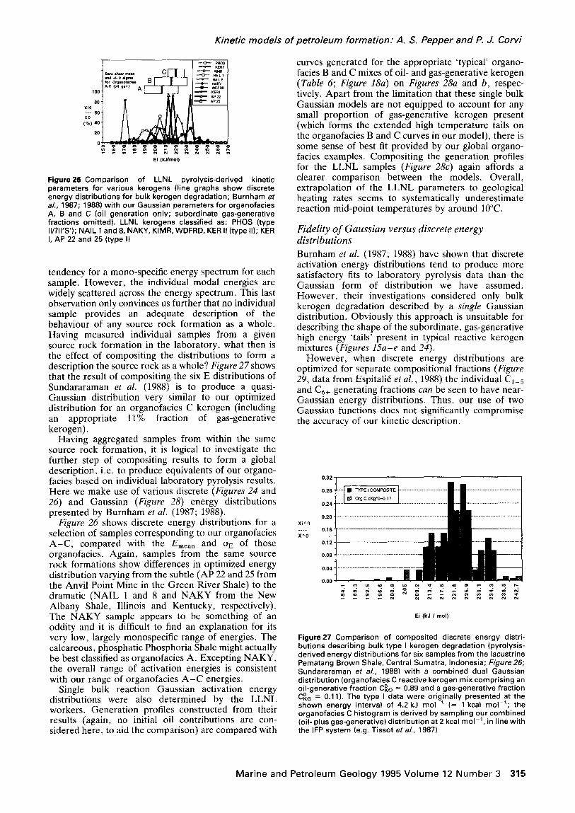
Figure 26 Comparison of LLNL pyrolysis-derived kinetic parameters for various kerogens (line graphs show discrete energy distributions for bulk kerogen degradation; Burnham et a/., 1987; 1988) with our Gaussian parameters for organofacies A, B and C (oil generation only; subordinate gas-generative fractions omitted). LLNL kerogens classified as: PHOS (type III?II’S’); NAIL 1 and 8, NAKY, KIMR, WDFRD, KER II (type II); KER I, AP 22 and 25 (type I)
tendency for a mono-specific energy spectrum for each sample. However, the individual modal energies are widely scattered across the energy spectrum. This last observation only convinces us further that no individual sample provides an adequate description of the behaviour of any source rock formation as a whole. Having measured individual samples from a given source rock formation in the laboratory, what then is the effect of compositing the distributions to form a description the source rock as a whole? Figure 27 shows that the result of compositing the six E distributions of Sundararaman er al. (1988) is to produce a quasi- Gaussian distribution very similar to our optimized distribution for an organofacies C kerogen (including an appropriate 11% fraction of gas-generative kerogen).
Having aggregated samples from within the same source rock formation, it is logical to investigate the further step of compositing results to form a global description, i.e. to produce equivalents of our organo- facies based on individual laboratory pyrolysis results. Here we make use of various discrete (Figures 24 and 26) and Gaussian (Figure 28) energy distributions presented by Burnham et al. (1987; 1988).
Figure 26 shows discrete energy distributions for a selection of samples corresponding to our organofacies A-C, compared with the E,,,, and on of those organofacies. Again, samples from the same source rock formations show differences in optimized energy distribution varying from the subtle (AP 22 and 25 from the Anvil Point Mine in the Green River Shale) to the dramatic (NAIL 1 and 8 and NAKY from the New Albany Shale, Illinois and Kentucky, respectively). The NAKY sample appears to be something of an oddity and it is difficult to find an explanation for its very low, largely monospecilic range of energies. The calcareous, phosphatic Phosphoria Shale might actually be best classified as organofacies A. Excepting NAKY, the overall range of activation energies is consistent with our range of organofacies A-C energies.
Single bulk reaction Gaussian activation energy distributions were also determined by the LLNL workers. Generation profiles constructed from their results (again, no initial oil contributions are con- sidered here, to aid the comparison) are compared with
0.20 Xi’0 __._ 0.16 X”0
0.12
0.08
0.32 , I
0.28
0.24
Kinetic models of petroleum formation: A. S. Pepper and P. J. Corvi
curves generated for the appropriate ‘typical’ organo- facies B and C mixes of oil- and gas-generative kerogen (Table 6; Figure 18a) on Figures 28a and b, respec- tively. Apart from the limitation that these single bulk Gaussian models are not equipped to account for any small proportion of gas-generative kerogen present (which forms the extended high temperature tails on the organofacies B and C curves in our model), there is some sense of best fit provided by our global organo- facies examples. Compositing the generation profiles for the LLNL samples (Figure 28~) again affords a clearer comparison between the models. Overall, extrapolation of the LLNL parameters to geological heating rates seems to systematically underestimate reaction mid-point temperatures by around 10°C.
Fidelity of Gaussian versus discrete energy distributions Burnham et al. (1987; 1988) have shown that discrete activation energy distributions tend to produce more satisfactory fits to laboratory pyrolysis data than the Gaussian form of distribution we have assumed. However, their investigations considered only bulk kerogen degradation described by a single Gaussian distribution. Obviously this approach is unsuitable for describing the shape of the subordinate, gas-generative high energy ‘tails’ present in typical reactive kerogen mixtures (Figures I.5a-e and 24).
However, when discrete energy distributions are optimized for separate compositional fractions (Figure 29, data from Espitalie et al., 1988) the individual C1_5 and Cg+ generating fractions can be seen to have near- Gaussian energy distributions. Thus, our use of two Gaussian functions does not significantly compromise the accuracy of our kinetic description.
Ei (kJ I mol)
Figure 27 Comparison of composited discrete energy distri- butions describing bulk type I kerogen degradation (pyrolysis- derived energy distributions for six samples from the lacustrine Pematang Brown Shale, Central Sumatra, Indonesia; Figure 26; Sundararaman et a/., 1988) with a combined dual Gaussian distribution (organofacies C reactive kerogen mix comprising an oil-generative fraction C”,o = 0.89 and a gas-generative fraction c”,, = 0.11). The type I data were originally presented at the shown energy interval of 4.2 kJ mol-’ (= 1 kcal mol-‘; the organofacies C histogram is derived by sampling our combined (oil- plus gas-generative) distribution at 2 kcal mol-‘, in line with the IFP system (e.g. Tissot et al., 1987)
Marine and Petroleum Geology 1995 Volume 12 Number 3 315

Kinetic models of petroleum formation: A. S. Pepper and P. J. Corvi
BP ‘B’ VS. LLNL gaussian Type II BP ‘c’ vs. LLNL gaussian Type I BP B&C vs. LLNL Type It/l ‘composites’
- LLNLNAILB - LLNLNAKY - LLNLKIM - LLNLPHOS
_._ 80 100 120 140 160 180 200 -‘-80 100 120 140 180 180 200 80 100 120 140 160 180 200
T (C) @ 2 C/Ma T (C) 8 2 C I Ma T (C) 8 2 C/Ma
Figure 28 Comparison of pyrolysis-derived kinetic predictions for type II and I kerogens (single Gaussian energy distributions describing bulk kerogen degradation from LLNL; Burnham et al., 1987; 1988) with our global model for typical members of organofacies B and C: (a) individual LLNL type II predictions versus BP global ‘typical’ organofacies B prediction; (b) individual LLNL type I predictions versus BP global ‘typical’ organofacies C prediction; and (c) cornposited LLNL types II and I predictions versus BP global ‘typical’ organofacies B and C, respectively
Guidelines for assigning kinetic parameters 3. Assign organofacies based on steps 1 and 2, using in frontier settings Table 1, etc.
Having designed a kerogen kinetic classification requir- ing only basic geological knowledge, our results are equally applicable in ‘geochemical frontiers’, as well as in basins where calibrant geochemical data might allow ‘fine-tuning’ of the predicted outcome. Even if alterna- tive geological models persist in the early stages of exploration analysis (e.g. the likelihood of organofacies D/E versus F in topset coals on a post-Palaeozoic passive margin), sensitivity studies may still allow the range of exploration outcomes to be narrowed down.
A typical series of steps in assigning kinetic and compositional parameters for modelling might be:
1. Locate the petroleum system in which the potential source rock is anticipated, and determine its age
2. Perform sequence analysis, break out GDE based on seismic geometries and attributes and, where available, lithofacies in adjacent wells or outcrops (Figure 5)
4. Assign initial geochemical characteristics using default values for the organofacies (Table 6). Estimate the likely initial kerogen composition using Equations (1) -(5).
Conclusions Oil and gas generation can be predicted in environ- ments of low knowledge using global kinetic para- meters. Our scheme uses the gross depositional environment and stratigraphic age to define five kerogen organofacies, individually characterized by a specific organic matter input, in addition to a depositional/early diagenetic overprint. They can generally be related to broad sedimentary facies:
A
B
C
D/E
F
Aquatic, marine environment, siliceous or car- bonate/evaporate lithofacies, any age Aquatic, marine environment, siliclastic litho- facies, any age Aquatic, non-marine, lacustrine environment, Phanerozoic Terrigenous, non-marine, ever-wet coastal environment, Mesozoic and younger Terrigenous, non-marine, coastal environment, late Palaeozoic and younger
1.0
0.8
xi”0 0.6
____
X”0 0.4
0.2
0.0
1 ??Draupne gas 1
Ei (kJ/mol)
Figure 29 Laboratory pyrolysis-derived discrete activation energy distributions for separate oil- and gas-generative kerogen components of a Draupne Formation sample, North Sea Basin (Espitalie et al., 1988). Although the energy distribu- tion of the total kerogen is distinctly non-Gaussian, it can be approximated closely by the product of two separate Gaussian distributions
We use routine pyrolysis and pyrolysis-GC data to divide immature organic carbon into four carbon components: initial oil, oil-generative, gas-generative and inert. Oil- and gas-generative fractions degrade independently, allowing us to compute both the con- centration and composition of generated hydrocarbons with increasing thermal stress.
We found optimum values for the required ten (5 x 2) kinetic parameter sets using a proprietary non- linear regression routine designed to fit Gaussian activation energy distributions to data sets spanning the requisite 12 orders of magnitude in heating rate between field and laboratory.
Differences in kinetic parameters for the five organo- facies are broadly consistent with their known chemical properties, although our knowledge is still too crude to
316 Marine and Petroleum Geology 1995 Volume 12 Number 3

construct kinetic models from first principles. Activa- tion energies for oil generation increase systematically in the order A-F, and this is expressed in a consistent increase in the temperature ranges over which oil is generated.
Kinetic models of petroleum formation: A. S. Pepper and P. J. Corvi
Anthony, D. B. and Howard, J. B. (1976) Coal devolatilisation and degasification AlChE J. 22, 625-656
Avni, E., Coughlin, R. W., Solomon, P. Ft. and King, H. H. (1985) Mathematical modelling of lignin pyrolysis fuel 64, 1495-1501
At a reference heating rate of 2°C Ma-‘, the OGW (temperature range over which 10 and 90% oil- generative kerogen has degraded) increases in the order organofacies A to F from ca. 95-135X to 145-175°C. The corresponding shift in the GGW (similar definition) is from ca. 105-155°C to 175-220°C.
Heating rate (i.e. time) also affects the temperature thresholds at which these reactions occur: as a general rule of thumb, an order of magnitude increase (decrease) in heating rate increases (decreases) the temperatures at which petroleum is generated by ca. 15°C. Because of the compensating effect of time and temperature, it is often necessary to consider thermal stress, rather than pure temperature. Natural heating rates in sedimentary basins can vary by almost two orders of magnitude: a source rock heated slowly to 130°C on a passive margin (0.5”C Ma-‘) experiences the same level of thermal stress as one heated ra
P idly to
160°C in a Neogene rift basin (50°C Ma- ). The additional compounding effect of organofacies can be dramatic: A in the example passive margin would be at base OGW, whereas F in the Neogene rift would still be at OGT!
Bar, H., Ikan, R. and Alzenshtat, Z. A. (1988a) Comparative study of the isothermal pyrolysis kinetic behaviour of some oil shales and coals J.Anal. Appl. Pyrol. 14, 49-71
Bar, H.. Ikan. R. and Alzenshtat. Z. (1988b) Fossil fuels and synthetic polymers: isothermal pyrolysis kinetics as indica- tion of structural resemblance J. Anal. Appf. Pyrol. 14,73-79
Barley, B. J., Chergotis, D., Wilson, M. and Young, S. (1992) Lithology prediction by extrapolating well data. In: Proceed- in.qs, Indonesian Petroleum Association 2 1st Annual Conven- tion, October 1992, 287-308
Baskin. D. K. and Peters. K. E. (1992) Earlv oeneration charac- teristics of a sulfur-rich Monterey kerogen”Am. Assoc. Petrol. Geol. Bull. 76, I- 13
Behar, F. and Pelet, R. (1985) Pyrolysis gas chromatography applied to organic geochemistry. Structural similarities between kerogens and asphaltenes from related rock extracts and oils J. Anal. Appl. Pyrol. 8, 173-187
Behar. F.. Pelet. R. and Roucache. J. (1985) Geochemistrv of asphaitenes.. In: Advances in Organic Geochemistry, Vol. 6 (Ed. P.A. Schenck), 587-585
Bertrand, P., Martinez, L. and Pradier, B. (1987) Petrologic study of primary migration by hydrous pyrolysis. In: Migration of Hydrocarbons in Sedimentary Basins (Ed. B. Doligez), Editions Technip, Paris, 633-647
Bjerey, M., Hall, P. B., Loberg, R., McDermott, J. A. and Mills, N. (1988) Hydrocarbons from non-marine source rocks. Adv. Org. Geochem. 13, 221-244
Bjoroy, M., Hall, K., Hall, P. B. and Leplat, P. (1992) Detailed hydrocarbon analyser for well site and laboratory use Mar. Petrol. Geol. 9, 648-665
Global temperature thresholds for oil and gas generation therefore constitute blunt instruments with which to assess the petroleum potential of sedimentary basins. Furthermore, knowledge of the temperature ranges over which oil and gas are generated is only partly useful. Because generated oil is itself potentially subject to thermal degradation in the source rock, a complete description of petroleum formation must couple descriptions of generation, oil-gas cracking and expulsion. For example, a generation model in isola- tion cannot account for the frequently observed association between gas provinces and coals.
Bostick, N. H. (1973) Time as a factor in thermal metamorphism of phytoclasts (coaly particles). Congres international de Stratigraphie et de Geologie du Carbonifere, Septieme, Krefeld, 23-28 August, 1971. Compte Rendu 2, 183-193
Braun, R. L. and Burnham, A. K. (1986) Kinetics of Colorado oil shale ovrolvsis in a fluidised-bed reactor Fuel 65, 218-222
Braun, R: L. and Burnham, A. K. (1987) Analysis of chemical reaction kinetics using a distribution of activation energies and simpler models Ener. Fuels 1, 153-161
Braun, R. L. and Rothman, A. J. (1975) Oil shale pyrolysis: kinetics and mechanism of oil production Fuel 54, 129-131
Bray, E. E. and Evans, E. D. (1961) Distribution of n-paraffins as a clue to recognition of source beds Geochim. Cosmochim. Acta 22, 2- 15
Acknowledgments We thank the management of BP Exploration for permission to publish; our colleagues, too numerous to mention individually, who contributed data and/or lively debate during the study; Dr C. Lilley for helping retrieve the mothballed MINEX code; Dr M. Gibbons and an anonymous IFP reviewer for helpful technical and editorial comments on the first draft; R. Davis, I. Longley and Dr B. Barley for additional comments on a later draft; Misran and the Jakarta drawing office; and Agus and Ade for technical assistance. ASP appreciates the support and patience of ICP, KJP and RCP.
Burnham, A. K. and Braun, R. L. (1985) General kinetic model for oil shale pyrolysis ln Situ 9, l-23
Burnham. A. K.. Braun. R. L.. Greaa. H. R. and Samoun. A. M. (1987). Comparison. of methi& for measuring kerogen pyrolysis rates and fitting kinetic parameters Ener. Fuels 1, 452-458
Burnham, A. K., Braun, R. L. and Samoun, A. M. (1988) Further comparison of methods for measuring kerogen pyrolysis rates and fitting kinetic parameters. In: Advances in Organic Geochemistrv 1987, Part // lEds L. Nattavelli and L. Novelli). Pergamon Press, Oxford, 839-846
Chenet, P. Y. (1984) Thermal transfer in sedimentary basins: palaeo-temperature reconstruction and maturation studies in the Gulf of Lion marain. In: Thermal Phenomena in Sedimentary Basins (Ed. BrDurand), Editions Technip, Paris, 257-270
References Akihisa, K. (1978) Etude cinetique des roches meres, rapport 4:
formation de produits petroliers par pyrolyse du kerogene a basse temperature J. Jpn. Assoc. Petrol. Technol. 44, 26-33
Albrecht, P. (1969) Constituents organiques des roches sedi- mentaires: etude de la diagenese dans un serie sedimentaire epaisse PhD Thesis, Univ. Strasbourg
Allen, P. A. and Allen, J. R. (1990) Basin Analysis: Principles and Applications, Blackwell Scientific, Oxford, 451 pp
Connan, J. (1974) Time-temperature relation in oil genesis Am. Assoc. Petrol. Geol. Bull. 58, 2516-2521
Cooles, G. P., Mackenzie, A. S. and Quigley, T. M. (1986) Calculation of petroleum masses generated and expelled from source rocks Or-u. Geochem. 10, 235-245
Daly, A. R. and Peters,-K. E. (1982) Continuous detection of pyrolytic carbon monoxide: a rapid method for determing sedimentary organic facies Am. Assoc. Petrol. Geof. Bull. 86, 2672-2681
Dow, W. G. (1977) Kerogen studies and geological interpreta- tions J. Geochem. Expl. 7,79-99
Durand, B. (1980) Sedimentary organic matter and kerogen. Definition and quantitative importance of kerogen. In: Kerogen, Insoluble Organic Matter from Sedimentary Rocks (Ed. B. Durand), Editions Technip, Paris, 13-34
Marine and Petroleum Geology 1995 Volume 12 Number 3 317

Kinetic models of petroleum formation: A. S. Pepper and P. J. Corvi
Durand, B. and Paratte, M. (1983) Oil potential of coals: a geochemical approach. In: Petroleum Geochemistry and Exploration of Europe (Ed. J. Brooks), Blackwell Scientific, Oxford, 285-292
Laplante, R. E. (1974) Hydrocarbon generation in Gulf Coast Tertiary sediments Am. Assoc. Petrol. Geol. Bull. 56, 1281-1289
Durand, B., Hut, A.-Y. and Oudin, J. L. (1987) Oil saturation and primary migration: observations in shales and coals from the Kerbau wells, Indonesia. In: Migration of Hydrocarbons in Sedimentary Basins (Ed. B. Doligez), Editions Technip, Paris, 173-196
Larter, S. R. and Senftle, J. T. (1985) Pyrolysis gas chroma- tography Nature 318, 277-280
Leavit-t, D. R., Tyler, A. L. and Kafesjian, A. S. (1987) Kerogen decomposition kinetics of selected Green River and Eastern U.S. oil shales from thermal solution experiments Ener. Fuels 1,520-525
Erdman, J. G. (1975) Time and temperature relations affecting the origin, expulsion and preservation of oil and gas. In: Proceedings, 9th World Petroleum Congress, Vol. 2, 139-148
Lewan, M. D. (1985) Evaluation of petroleum generation by hydrous pyrolysis experimentation Phil. Trans. R. Sot. London A 315,123-134
England, W. A., Mackenzie, A. S., Quigley, T. M. and Mann, D. M. (1987) The movement and entrapment of petroleum fluids in the subsurface J. Geol. Sot. London 144,327-347
Espitalie, J., Laporte, J. L., Madec, M., Marquis, F., Leplat, P., Paulet. J. and Boutefeu. A. (1977) Methode: rapide de characterisation des roches meres, leur potentiel petrolier et de leur degre d’evolution Rev. inst. Fr. Petrol. 32, 23-42
Espitalie, J., Ungerer, P., Irwin, I. and Marquis, F. (1988) Primary cracking of kerogens: experimenting and modeliing C,, C.&s, Cs-C14 and C,s+ classes of hydrocarbon formed Org.. Geochem. 13,893-899
Lewan, M. D. and Williams, J. A. (1987) Evaluation of petroleum generation from resinites by hydrous pyrolysis Am. Assoc. Petrol. Geol. Bull. 71, 207-214
Lewan, M. D., Winters, J. C. and McDonald, J. H. (1979) Generation of oil-like pyrolysates from organic-rich shales Science 203.897-899
Longley, I. M., Barraclough, R., Bridden, M. A. and Brown, S. (1990) Pematang lacustrine petroleum source rocks from the Malacca Strait PSC, Central Sumatra, Indonesia. In: Proceed- ings, Indonesian Petroleum Association, 19th Annual Convention, October 1990,279-297
Espitalie, J., Marquis, F., Drouet, S. and Lafargue, E. (1991) Critical study of modelling parameters [abstract]. In: Pro- ceedings of International Conference on Basin Modelling: Advances and Applications, Stavanger, March 1991, 17
Evans, D. J., Menelly, A. and Brown, G. (1992) Seismic facies analysis of Westphalian sequences of the southern North Sea Mar. Petrol. Geoi. 9, 578-589
Fielding, C. R. (1985) Coal depositional models and the distinc- tion between alluvial and delta plain environments Sedim. Geol. 42,41-48
Lopatin, N. V. (1971) Temperatura i geologicheskoe vremya kak faktorv uolefikatsii Izv. Acad. Nauk SSSR, Ser. Geof. 3. 95-Id6 -
Louis, M. C. and Tissot, B. P. (1967) Influence de la temperature et de la pression sur la formation de hydrocarbures dans les argiles a kerogene. In: Proceedings, 7th World Petroleum Congress, Mexico, Vol. 2,47-60
Luheshi, M. N. (1983) Estimation of formation temperature from borehole measurements Geophys. J. R. Astron. Sot. 74, 747-766
Forbes, P. L., Ungerer, P. M., Kuhfuss, A. B., Riis, F. and Eggen, S. (1991) Compositional modelling of petroleum generation and expulsion. Application to a three dimensional balance in the Smorbukk Beta field Am. Assoc. Petrol. Geol. Bull. 75, 873-893
McNab, J. G., Smith, P. V., Jr and Betts, R. L. (1952) The evolution of petroleum lnd. Engin. Chem. 44, 2556-2563
Mackenzie, A. S. and Quigley, T. M. (1988) Principles of geochemical prospect appraisal Am. Assoc. Petrol, GeoL Bull. 72, 399-415
Galloway, W. E. and Hobday, D. K. (1983) Terrigenous Clastic Depositional Systems, Springer Verlag, Berlin
Guidish, T. M., Kendall, C. G. StC., Lerche, I., Toth, D. J. and Yarzab, Ft. F. (1985) Basin evaluation using burial history calculation: an overview Am. Assoc. Petrol. Geol. Bull. 69, 92-105
Hartman-Stroup, C. (1987) The effect of organic matter type and organic carbon content on Rock-Eva1 hydrogen index in oil shales and source rocks Org. Geochem. 11,351-369
Harwood, R. J. (1977) Oil and gas generation by laboratory pyrolysis of kerogen Am. Assoc. Petrol. Geol. Bull. 61, 2082-2102
Momper, J. A. (1972) Evaluating source beds for petroleum [abstract] Am. Assoc. Petrol. Geol. Bull. 56, 640
Monnier, F., Powell, T. G. and Snowdon, L. R. (1981) Qualitative and quantitative aspects of gas generation during matura- tion of sedimentary organic matter: examples from Canadian frontier basins Adv. Org. Geochem. 1981,487-495
Mukhopadhyay, P. K. and Gormly, J. R. (1984) Hydrocarbon potential of two types of resinite Org. Geochem. 6,439-454
Morley, R. J. (1981) Development and vegetation dynamics of a lowland ombrogenous peat swamp in Kalimantan Tengah, Indonesia J. Biogeog. 8, 383-404
Hoering, T. C. and Abelson, P. H. (1963) Hydrocarbons from kerogen Carnegie Institute, Washington Yearbook 62, 229-234
Nielsen, S. B. (1991) The reliability of kerogen kinetic models [abstract]. In: Proceedings of International Conference on Basin Modefling: Advances and Applications, Stavanger, March 1991, 18
Hood, A., Gutjahr, C. C. M. and Heacock, R. L. (1975) Organic metamorphism and the generation of petroleum Am. Assoc. Petrol. Geol. Bull. 59.986-996
Hut, A.-Y., Durand, B., Roucachet, J., Vandenbroucke, M. and Pittion, J. L. (1986) Comparison of three series of organic matter of continental origin Org. Geochem. 10, 65-72
Huck, G. and Karwell, J. (1955) Physicalische probleme der inkohlung Brennstoh-Chem. 36, l-11
Hunt, J. M., Lewan, M. D. and Hennet, R. J. C. (1991) Modelling oil generation with time-temperature index graphs based on the Arrhenius equation Am. Assoc. Petrol. Geol. Bull. 75, 795-807
Nip, M., De Leeuw, J. W., Schenck, P. A., Windig, W., Meuzelaar, H. L. C. and Crelling, J. C. (1989) A flash pyrolysis and petrographic study of cutinite from the Indiana paper coal Geochim. Cosmochim. Acta 53, 671-683
Okul, A. and Waples, D. W. (1992) The influence of oil expulsion efficiency on the type of hydrocarbons accumulating in traps. In: Proceedings, Offshore SE Asia, 9th Conference and Exhibition, l-2 December 1992, 685-698
Orr, W. L. (1986) Kerogen/asphaltene/sulphur relationship in sulphur-rich Monterey oils In: Advances in Organic Geochemistry 1985, Vol. 10 (Eds D. Leythaeuser and J. Rullkotter), 499-516
Juntgen, H.and van Heek, K. H. (1968) Gas release from coal as a function of the rate of heating Fuel 48, 103- 117
Karwell, J. (1955) Die metamorphose der kohlen vom stand- punkt der phisikalischen chemie Dtsch GeoL Gesell. Zeitschr. 107,132-139
Pepper, A. S. (1989) Petroleum expulsion behaviour of source rocks: a novel perspective [abstract]. In: Proceedings, 14th International Meeting on Organic Geochemistry, Paris, 18-22 September 1989
Katz, B. J. (1990) Controls on the distribution of lacustrine source rocks through time and space. In: Lacustrine Basin Exploration (Ed. B. J. Katz), Am. Assoc. Petrol. Geol Mem. Nci 50, 132-139
Klemme, H. D. and Ulmishek, G. F. (1991) Effective petroleum source rocks of the world: stratigraphic distribution and controlling depositional factors Am. Assoc. Petrol. Geol. Bull. 75, 1809-1851
Pepper, A. S. (1992) Estimating the petroleum expulsion behaviour of source rocks: a novel quantitative approach. In: Petroleum Migration (Eds A. J. Fleet and W. A. England), Spec. Publ. Geol. Sot. London No. 59,9-31
Pepper, A. S. and Corvi, P. J. Simple kinetic models of petroleum formation, Part Ill: simulating an open system. Mar. Petrol. Geol., in press
Pepper, A. S. and Dodd, T. A. (1995) Simple kinetic models of petroleum formation. Part II: oil-gas cracking Mar. Petrol. Geof. 11, 321-340
318 Marine and Petroleum Geology 1995 Volume 12 Number 3
Peters, K. E. (1986) Guidelines for evaluating petroleum source rocks using programmed pyrolysis Am. Assoc. Petrol. Geol. Bull. 70, 318-329
Kinetic models of petroleum formation: A. S. Pepper and P. J. Corvi
Thompson, S., Morley, R. J., Barnard, P. C. and Cooper, B. S. (1985) Facies recoanition of some Tertiarv coals aoolied to prediction of oil so:rce rock occurrence Mar. Petrol Gee/. 2, 288-297 Philippi, G. T. (1965) On the depth, time and mechanism of
petroleum generation Geochim. Cosmochim. Acta 29, 1021-1049
Pitt, G. J. (1961) The kinetics of the evolution of volatile products form coal. In: 4th International Conference on Coal Science, Le Touquet, France, 30 May-2 June 1961
Powell, T. G. (1986) Petroleum geochemistry and depositional setting of lacustrine source rocks Mar. Petrol. GeoL 3, 200-219
Tissot, B. P. (1969) Premieres donnees sur les mecanismes et la cinetique de la formation du petrole dans les sediments: simulation d’un schema reactionnel sur ordinateur Rev. Inst. Fr. Petrol. 24, 470-501
Powell, T. G. and Boreham, C. B. (1994) Terrestrially sourced oils: where do they come from and what are our limits to knowledge? In: Coal and Coal-bearing Strata as Oil-prone Source Rocks (Eds. A. C. Scott and M. J. Fleet), Spec. Pub/. Geol. Sot. London No. 77, II -29
Quigley, T. M. and Mackenzie, A. S. (1988) The temperatures of oil and gas formation in the sub-surface Nature 333,549-552
Quigley, T. M., Mackenzie, A. S. and Gray, J. R. (1987) Kinetic theory of petroleum generation. In: Migration of Hydro- carbons in Sedimentary Basins (Ed. B. Doligez), Editions Technip, Paris, 649-665
Tissot, B. P. and Espitalie, J. (1975) L’evolution de la matiere organique des sediments: application d’une simulation mathematique Rev. Inst. Fr. Petrol. 30, 743-777
Tissot, B. P., Califet-Debyser, Y., Deroo, G. and Oudin, J. L. (1971) Oriain and evolution of hvdrocarbons in Earlv Toarcian siales Am. Assoc. Petrol. Gebf. Bull. 55,2177-2193
Tissot, B., Durand, B., Espitalie, J. and Combaz, A. (1974) Influence of nature and diagenesis of organic matter in formation of petroleum Am. Assoc. Petrol. Geol. Bull. 58, 499-506
Tissot, B. P., Deroo, G. and Hood, A. (1978) Geochemical study of the Uinta Basin: formation of petroleum from the Green River Formation Geochim. Cosmochim. Acta 42, 1469-1485
Saxby, J. D. and Riley, K. W. (1984) Petroleum generation by laboratory-scale pyrolysis over six years simulating con- ditions in a subsiding basin Nature 308, 177-179
Saxby, J. D., Bennet, A. J. R., Corcoran, J. F., Lambert, D. E. and Riley, K. W. (1986) Petroleum generation: simulation over six years of hydrocarbon formation from torbanite and brown coal in a subsiding basin Org. Geochem. 9, 69-81
Serio, M. A., Hamblen, D. G., Markam, J. R. and Solomon, P. R. (1987) Kinetics of volatile product evolution in coal pyrolysis: experiment and theory Ener. Fuels 1, 138-152
Shanmugam, G. (1985) Significance of coniferous rain forests and related organic matter in generating commercial quan- tities of oil, Gippsland Basin, Australia Am Assoc. Petrol. Geol. Bull. 89, 1241- 1254
Tissot, B. P., Pelet, R. and Ungerer, P. (1987) Thermal history of sedimentary basins, maturation indices and kinetics of oil and gas generation Am. Assoc. Petrol. Geof. Bull. 71, 1445-1466
Ungerer, P. (1984) Models of petroleum formation: how to take into account geology and chemical kinetics. In: Thermal Phenomena in Sedimentary Basins (Ed. B. Durand), Editions Technip, Paris, 235-246
Ungerer, P. (1985) Notice d’utilisation du programme OPTIM Rep. 33388, lnstitut Francais du P&role, Paris
Ungerer, P. and Pelet, R. (1987) Extrapolation of the kinetics of oil and gas formation from laboratory experiments to sedimentary basins Nature 27, 52-54
Ungerer, P., Bessis, F., Chenet, P.Y., Durand, B., Nogaret, E., Chiarelli, A., Oudin, J. L. and Perrin, J. F. (1984) Geological and geochemical models in oil exploration: principles and practical examples. In: Petroleum Geochemistry and Basin Evaluation (Ed. G. Demaison), Am. Assoc. Petrol. Geol. Mem. No. 35, 53-77
Snowdon, L. R. (1979) Errors in extrapolation of experimental kinetics parameters to organic geochemical systems Am. Assoc. Petrol. Geof. Bull. 83, 1128-l 134
Snowdon, L. R. and Powell, T. G. (1982) Immature oil and condensate - modification of hydrocarbon generation model for terrestrial organic matter Am. Assoc. Petrol. Geol.
- Bull. 88, 775-788 Stack, E., Mackowsky, M. Th., Teichmuller, M., Taylor, G. H.,
Chandra, D. and Teichmuller, R. (1975) Stach’s Textbook of Coal Petrology, Gebruder Borntraeger
Stevens, N. P., Bray, E. E. and Evans, E. D. (1956) Hydrocarbons in sediments of Gulf of Mexico Am. Assoc. Petrol. Geol. Bull. 46975-983
Stout, S. A., Boon, J. J. and Spackman, W. (1988) Molecular aspects of the peatification and early coalification of angio- sperm and gymnosperm woods Geochim. Cosmochim. Acta 52,405-414
Sundararaman, P., Teerman, S. C., Mann, R. G. and Mertani, B. (1988) Activation energy distribution: a key parameter in basin modelling and a geochemical technique for studying maturation and organic facies. In: Proceedings, Indonesian Petroleum Association, 17th Annual Convention, October 1988, 169-185, IPA-88-11.28
Sweeney, J. J. (1988) Application of maturation indicators and oil reaction kinetics -to put constraints on thermal history models of The Uinta Basin, Utah. U.S.A. Ora. Geochem. 13. 199-205
Sweeney, J. J., Burnham, A. K. and Braun, R. L. (1986) A model of hydrocarbon maturation in the Uinta Basin, Utah, USA. In: Thermal Modelling in Sedimentary Basins (Ed. J. Burns), Editions Technip, Paris, 547-561
Sweeney, J. J., Burnham, A. K. and Braun, R. L. (1987) A model of hydrocarbon generation from Type I kerogen: application to Uinta Basin, Utah Am. Assoc. Petrol. Geof. Bull. 71, 967-985
Tannenbaum, E. and Aizenshtat, 2. (1985) Formation of immature asphalt from oraanic-rich carbonate rocks I: geochemical correlation Org.-Geochem. 8, 181-192
Teichmuller. R.. Teichmuller. M. and Bartenstein. H. (1971) Umwandlung der organischen substanz in dach des Bramschen Massivs Fortschr. Geol. Rheinland Westfalen 18, 501-538
Ungerer, P., Espitalie, J., Marquis, F. and Durand, B. (1986) Use of kinetic models of organic matter evolution for the reconstruction of paleotemperatures: application to the case of the Gironville well (France). In: Thermal Phenomena in Sedimentary Basins, Editions Technip, Paris, 531-537
Vail, P. R. (1987) Seismic stratigraphy interpretation using sequence stratigraphy. In: Atlas-of Seismic Stratigraphy, Vol. 1 IEd. A. W. Ballv). Am. Assoc. Petrol. Geol. Stud. GeoL No. 7;. I-10 ‘..
Vandenbroucke, M. (1980) Structure of kerogens as seen by investigations on soluble extracts. In: Kerogen, insoluble Organic Matter from Sedimentary Rocks (Ed. B. Durand), Editions Technip, Paris, 415-443
van Krevelen, D. W. (1961) Coal, Elsevier, New York van Waaoner, J. C., Posamentier, H. W., Mitchum, R. M., Vail,
P. R.:Sarg, J. F., Loutit, T. S. and Hardenbol, J. (1988) An overview of sequence stratigraphy and key definitions. In: Sea-level Changes: an Integrated Approach (Eds C. W. Wilgus, B. J. Hastings, H. Posamentier, J. C. Van Wagoner, C. A. Ross and C. G. St.C. Kendall), Spec. Pub/. Sot. Econ. Palaeontol. Mineral. No. 42, 39-45
Vasseyovich, N. B., Korchagina, Yu I., Lopatin, N. V. and Chernyshev, V. V. (1970) Principle phase of oil formation lnt. Geol. Rev. 12,1276-1296
Waples, D. W. (1980) Time and temperature in petroleum formation: application of Lopatin’s method to petroleum exploration Am. Assoc. Petrol. Geol. Bull. 64, 916-926
Weltkamp, A. W. and Gutberlet, L. C. (1968) Application of micro-retort problems in shale pyrolysis Am. Chem. Sot. Div. Petrol. Chem. Prepr. 13, F71-F85
Winters, J. C., Williams, J. A. and Lewan, M. D. (1983) A laboratory study of petroleum generation by hydrous pyrolysis. In: Advances in Organic Geochemistry 1981 (Eds M. Bjerey et al.), 524-533
Wood, D. A. (1988) Relationships between thermal maturity indices calculated using Arrhenius Equation and Lopatin method: implications for petroleum exploration Am. Assoc. Petrol. Geol. Bull. 72, 115- 135
Marine and Petroleum Geology 1995 Volume 12 Number 3 319