Embed Size (px)
Citation preview

Saket Sathe and Charu C. Aggarwal
IBM T J Watson Research Center
Yorktown, NY 10598
Similarity Forests
ACM KDD Conference, 2017

Introduction
• Random forests are among the most popular classificationmethods used by real-world data scientists because of theirextraordinary accuracy and effectiveness.
• A recent experimental comparison among more than 100classifiers placed these methods as the top-performing tech-niques together with SVMs.
• Their use is primarily limited to multidimensional data be-cause they sample features from the original data set.
• We propose a method for extending random forests to workwith any arbitrary set of data objects.
– The input is provided as similarities among the data ob-jects rather than as multidimensional features.
Motivation
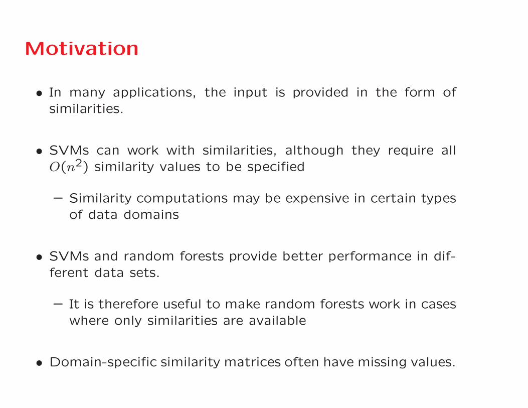
• In many applications, the input is provided in the form ofsimilarities.
• SVMs can work with similarities, although they require allO(n2) similarity values to be specified
– Similarity computations may be expensive in certain typesof data domains
• SVMs and random forests provide better performance in dif-ferent data sets.
– It is therefore useful to make random forests work in caseswhere only similarities are available
• Domain-specific similarity matrices often have missing values.

Contributions
• Design a random forest to work with similarity values rather
than multidimensional features.
• Requires the computation of only O(n · log(n)) similarity val-
ues.
• Can be used with missing values and noisy data sets.
• Can be used even in cases where the full dimensional repre-
sentation is available
– Provides competitive or slightly better performance than
traditional random forests
Notations
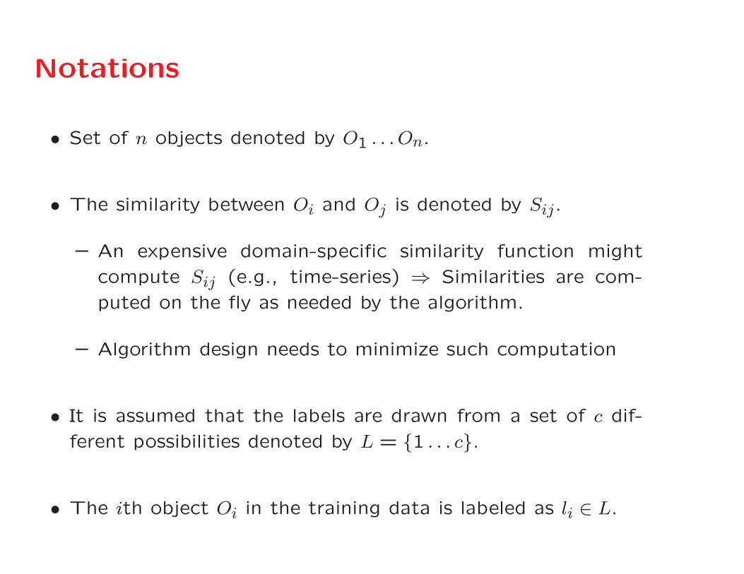
• Set of n objects denoted by O1 . . . On.
• The similarity between Oi and Oj is denoted by Sij.
– An expensive domain-specific similarity function might
compute Sij (e.g., time-series) ⇒ Similarities are com-
puted on the fly as needed by the algorithm.
– Algorithm design needs to minimize such computation
• It is assumed that the labels are drawn from a set of c dif-
ferent possibilities denoted by L = {1 . . . c}.
• The ith object Oi in the training data is labeled as li ∈ L.
Definition
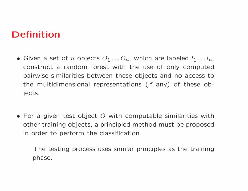
• Given a set of n objects O1 . . . On, which are labeled l1 . . . ln,
construct a random forest with the use of only computed
pairwise similarities between these objects and no access to
the multidimensional representations (if any) of these ob-
jects.
• For a given test object O with computable similarities with
other training objects, a principled method must be proposed
in order to perform the classification.
– The testing process uses similar principles as the training
phase.

SimForest: Broader Principles
• The basic idea is to assume that a multidimensional space
exists in which the objects can be embedded (but do not
explicitly compute it).
• Using kernel methods to extract a multidimensional repre-
sentation of the objects defeats the purpose.
– Such an approach can potentially use O(n2) space and
O(n3) time.
– Not practical for most real-world settings.
• All O(n2) pairs of similarities are not required to construct a
similarity forest.

Splitting with Similarity Values
• The objects O1 . . . On can be theoretically embedded in somemultidimensional space as the points X1 . . . Xn (not explicitlycomputed).
• Just as a random forest samples features from a multidimen-sional data set, the similarity-based approach samples pairs ofobjects in order to define directions in the multidimensionalspace.
– Sampling the object Oi and Oj results in the vector direc-tion from Xi to Xj.
• The data objects are then split into two groups using a hyper-plane perpendicular to this direction (all done without explicitprojection).
Recursive Splitting
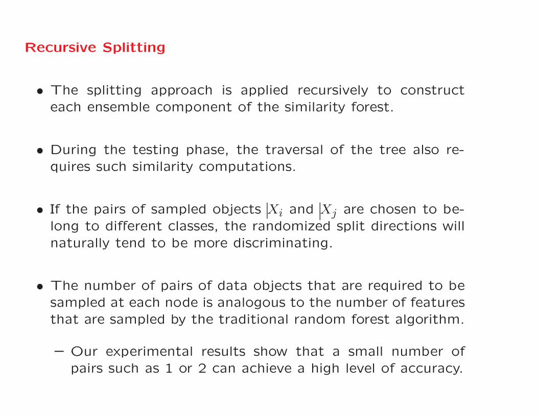
• The splitting approach is applied recursively to constructeach ensemble component of the similarity forest.
• During the testing phase, the traversal of the tree also re-quires such similarity computations.
• If the pairs of sampled objects Xi and Xj are chosen to be-long to different classes, the randomized split directions willnaturally tend to be more discriminating.
• The number of pairs of data objects that are required to besampled at each node is analogous to the number of featuresthat are sampled by the traditional random forest algorithm.
– Our experimental results show that a small number ofpairs such as 1 or 2 can achieve a high level of accuracy.
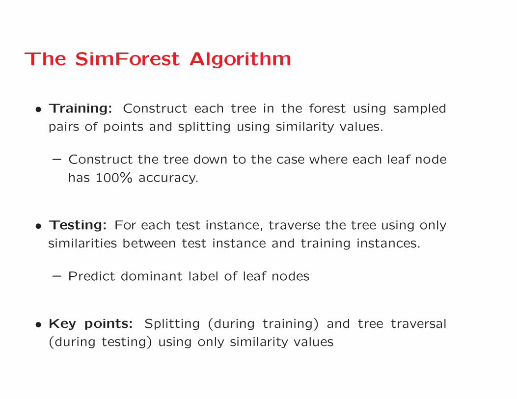
The SimForest Algorithm
• Training: Construct each tree in the forest using sampled
pairs of points and splitting using similarity values.
– Construct the tree down to the case where each leaf node
has 100% accuracy.
• Testing: For each test instance, traverse the tree using only
similarities between test instance and training instances.
– Predict dominant label of leaf nodes
• Key points: Splitting (during training) and tree traversal
(during testing) using only similarity values

Splitting
• Consider a pair of objects Oi and Oj that define the directionof the split.
• Consider an object Ok that needs to be projected along thisdirection.
• The unit direction of the embedding is given byXj−Xi
||Xj−Xi||.
• The projection P(Xk) of Xk on this direction is thereforegiven by the dot product of Xk −Xi on this unit direction.
P(Xk) = (Xk −Xi) ·Xj −Xi
||Xj −Xi||
• Need to express the above in terms of similarities!

Splitting
• One can express the numerator as dot products and then
replace with similarities:
P(Xk) =Xk ·Xj −Xk ·Xi −Xi ·Xj +Xi ·Xi
||Xj −Xi||=
Skj − Ski − Sij + Sii
||Xj −Xi||=
Skj − Ski − Sij + Sii√Sii + Sjj − 2Sij
• We already have a projection purely in terms of similarities,
and we can use it readily.
• But we can simplify even further!

Simplification
• The expression for projection can be simplified as follows:
P(Xk) =Skj − Ski − Sij + Sii√
Sii + Sjj − 2Sij
= A · (Skj − Ski) +B
• Here, A and B are constants that do not depend on the
object Ok being projected.
• We do not care about these constants–only the ordering of
the objects on the projection line.
• So we can simply use (Skj − Ski) to order the points for the
split!
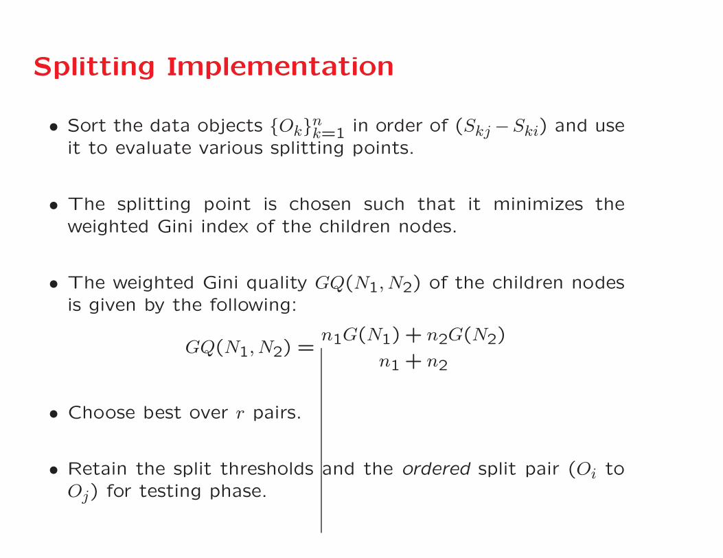
Splitting Implementation
• Sort the data objects {Ok}nk=1 in order of (Skj −Ski) and useit to evaluate various splitting points.
• The splitting point is chosen such that it minimizes theweighted Gini index of the children nodes.
• The weighted Gini quality GQ(N1, N2) of the children nodesis given by the following:
GQ(N1, N2) =n1G(N1) + n2G(N2)
n1 + n2
• Choose best over r pairs.
• Retain the split thresholds and the ordered split pair (Oi toOj) for testing phase.

Testing Phase
• The testing phase uses an identical approach to project thetest points on the line defined by the pairs of training pointsat each node.
• If (Oi,Oj) is the defining pair of objects for a given node,then the value of Skj − Ski is computed for the test objectOk.
• The stored split point (say a) is used to determine whichpath in the decision tree to follow depending on whether ornot Skj − Ski ≤ a.
• This step is performed for each node on the path of the tree,until the object Ok is assigned to a leaf node.
• The label of the leaf node is reported as the prediction.

Distances in lieu of Similarities
• In some settings, it is easier to compute distances rather than
similarities.
– In the sequence domain, one might naturally use the edit
distance or the dynamic time-warping distance.
• Natural solution: use cosine law with squared distance matrix
Δ
S = −1
2(I − U/n)Δ(I − U/n) (1)
• Disadvantage: Requires all pairs of distances ⇒ Loses some
of the efficiency properties of similarity forests

Simplified Approach
• The cosine law is not really required if one can make somesimplifying assumptions.
• Assumption: Each point is normalized to unit norm (mightnot be true in reality).
• Let D(Oi,Oj) be the distance between data points Oi andOj.
D(Ok,Oi)2 −D(Ok,Oj)
2 = ||Xk −Xi||2 − ||Xk −Xj||2= 2Xk ·Xj − 2Xk ·Xi + (||Xi||2 − ||Xj||2)︸ ︷︷ ︸
Zero (Because of Normalization)
∝ Skj − Ski
• So we can simply use the difference in squared distances forsplits instead of similarities!

Incompletely Specified Similarities
• Common problem in settings where similarity estimation is
expensive.
• If similarities between pairs of objects (such as images) are
obtained using crowd-sourcing, a cost may be incurred for
each pairwise similarity.
• Not all objects can be partitioned between a pair of nodes at
each split point.
– The projection of data points along arbitrary directions
may require unobserved similarities to be available.

Training with Incompletely SpecifiedSimilarities
• The selected pairs of objects (Oi,Oj) for splitting should al-
ways be such that similarity between them is observed. How-
ever, Ok may have unobserved similarities with either Oi or
Oj.
• Since Ok cannot be assigned to one of the child nodes, we
allow it to stay at the current node as its final destination.
• The class label of an internal node is defined by its majority
class.
• Unlike the case of fully observed similarities, internal nodes
also have a label.
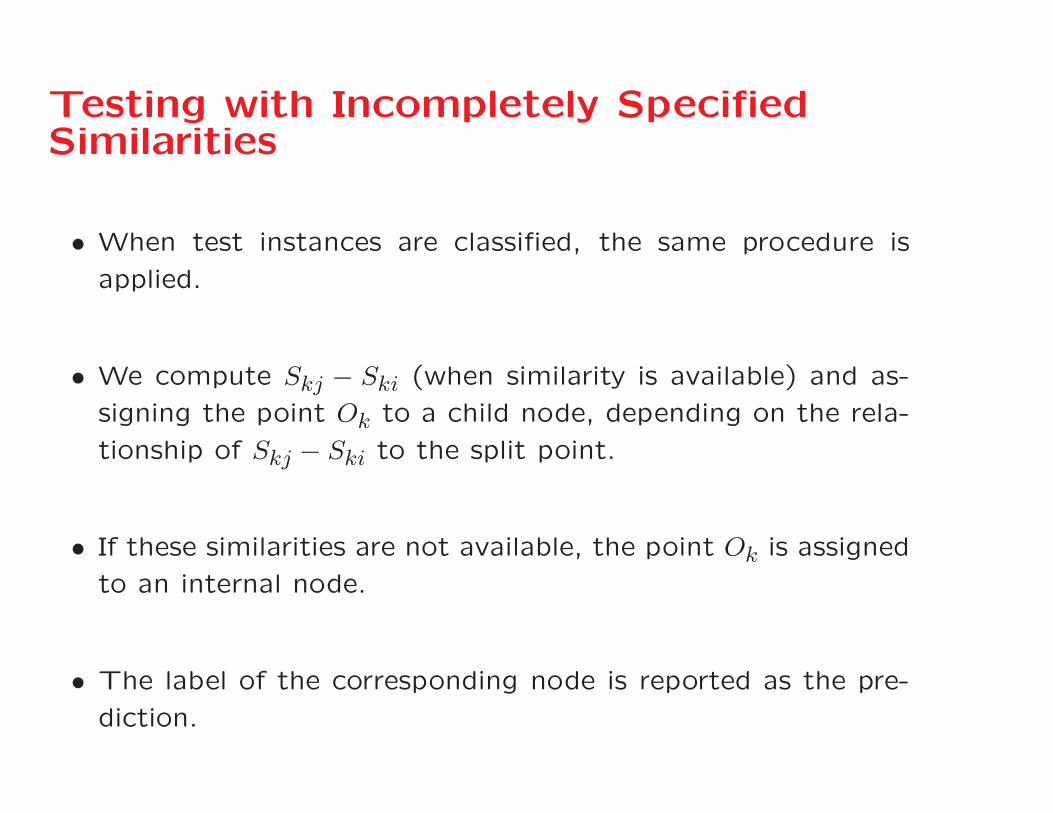
Testing with Incompletely SpecifiedSimilarities
• When test instances are classified, the same procedure is
applied.
• We compute Skj − Ski (when similarity is available) and as-
signing the point Ok to a child node, depending on the rela-
tionship of Skj − Ski to the split point.
• If these similarities are not available, the point Ok is assigned
to an internal node.
• The label of the corresponding node is reported as the pre-
diction.

Experimental Results
• Extensive experimental results comparing SimForest with
other competitive techniques.
• Extensively test SimForest’s resistance to noisy similarities.
• Evaluate how missing similarity values affect the accuracy of
SimForest.
• Show results on multidimensional data.

Similarity Matrix Generation
• Add noise to similarity matrix in controlled way with noise
coefficient α.
– Assume access to multidimensional data for building sim-
ilarity matrices but not to algorithm or baselines.
– Use cosine and RBF similarity on multidimensional data.
• Naturally used as kernels in support vector machines.
• SVMs are a natural baseline.
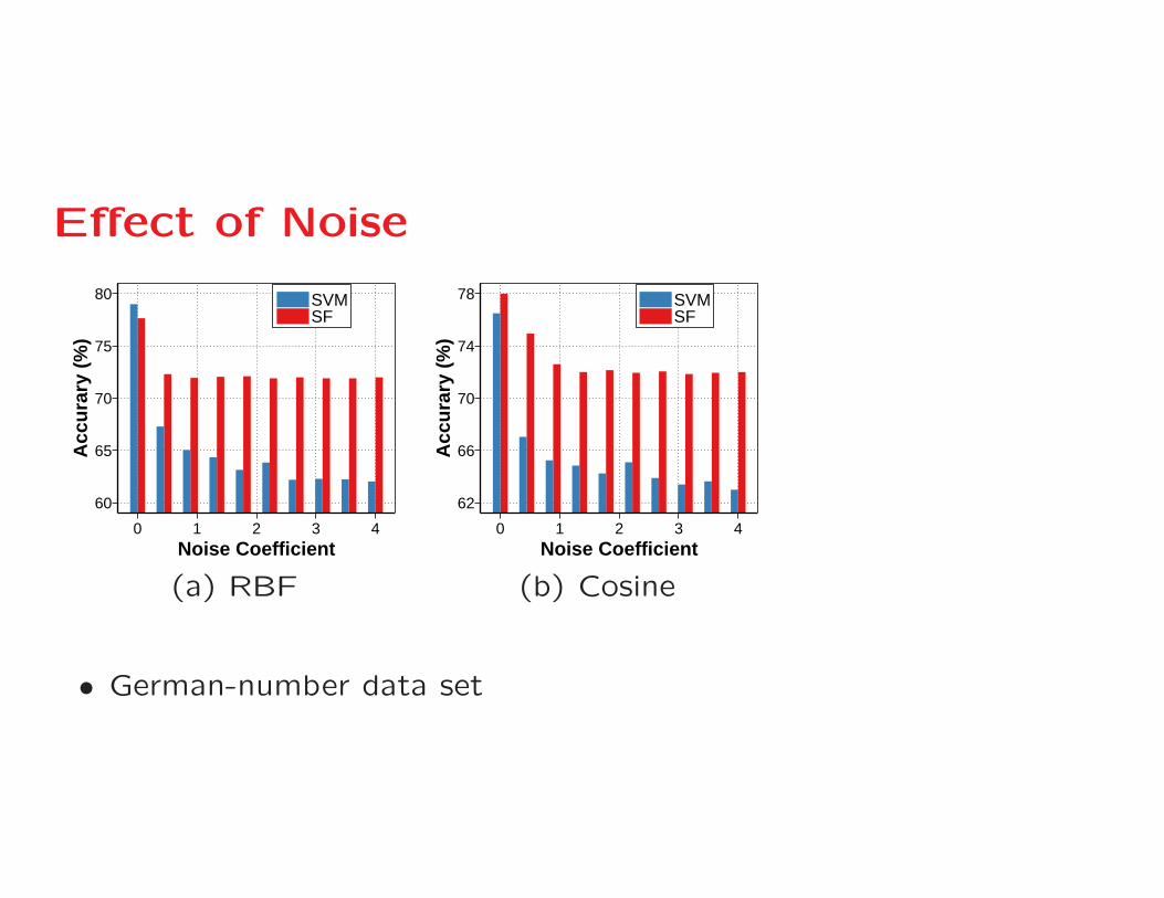
Effect of Noise
60
65
70
75
80
0 1 2 3 4Noise Coefficient
Acc
ura
ry (
%)
SVMSF
62
66
70
74
78
0 1 2 3 4Noise Coefficient
Acc
ura
ry (
%)
SVMSF
(a) RBF (b) Cosine
• German-number data set

Effect of Noise (Contd.)
65
70
75
80
85
0 1 2 3 4Noise Coefficient
Acc
ura
ry (
%)
SVMSF
71
73
75
77
79
81
83
0 1 2 3 4Noise Coefficient
Acc
ura
ry (
%)
SVMSF
(a) RBF (b) Cosine
• A1A data set

Fixed Noise LevelData set RBF Kernel Cosine Similarity
SimForest SVM SimForest SVMHeart 68.14 67.22 72.96 68.70Ionosphere 71.69 68.59 74.22 65.91Australian 61.88 61.23 85.79 79.49Diabetes 68.44 64.87 67.33 62.85German-Numer 72.00 62.80 71.85 65.40a1a 75.94 67.81 75.97 72.88
• Noise level fixed at α = 2.5
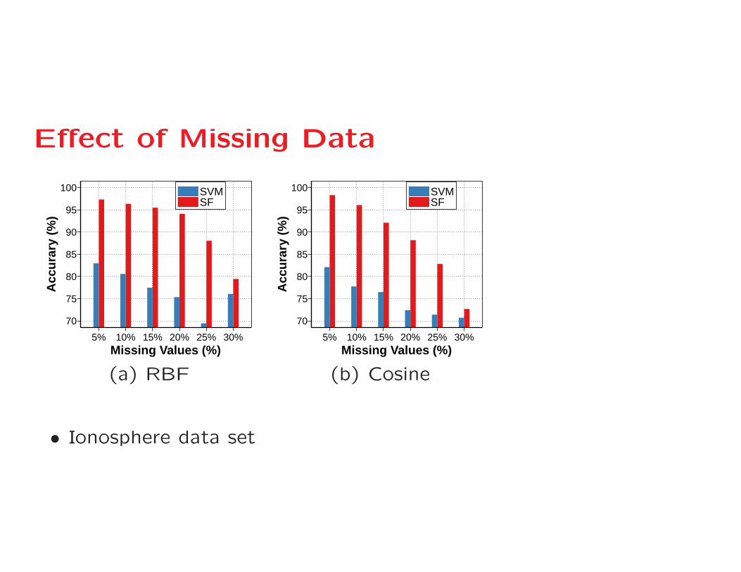
Effect of Missing Data
70
75
80
85
90
95
100
5% 10% 15% 20% 25% 30%Missing Values (%)
Acc
ura
ry (
%)
SVMSF
70
75
80
85
90
95
100
5% 10% 15% 20% 25% 30%Missing Values (%)
Acc
ura
ry (
%)
SVMSF
(a) RBF (b) Cosine
• Ionosphere data set

Effect of Missing Data
68
72
76
80
84
88
5% 10% 15% 20% 25% 30%Missing Values (%)
Acc
ura
ry (
%)
SVMSF
70
74
78
82
86
5% 10% 15% 20% 25% 30%Missing Values (%)
Acc
ura
ry (
%)
SVMSF
(a) RBF (b) Cosine
• Splice data set

Fixed Missing ValuesData set RBF Kernel Cosine Similarity
SimForest SVM SimForest SVMGerman-Numer 72.25 67.60 72.05 64.25Australian 90.14 83.47 89.63 86.23Ionosphere 95.49 77.46 92.11 76.47Breast-Cancer 97.00 90.94 96.42 92.07Madelon 56.11 53.91 55.65 53.11Splice 79.81 74.94 79.02 71.53
• Missing values fixed at 15%

Multidimensional dataData set Heart ION WBC GN SVMGuide3 a1a MushroomsSimForest 83.33 100.00 96.35 78.50 90.24 82.81 100.00Random Forest 79.62 94.36 96.35 77.00 87.80 82.63 100.00SVM 81.48 87.32 96.35 76.00 58.53 83.42 100.00
• Previous experiments only expose the similarity matrices to
the algorithms.
• SimForest can even be used for traditional multidimensional
data
• Provides competitive performance in such cases

Conclusions and Summary
• Propose SimForest, which can be used with traditional sim-
ilarity matrices
• Resistant to noise in the data
• Can work well with missing values
• Provides competitive performance for traditional multidimen-
sional data


![User profile correlation-based similarity (UPCSim) algorithm ......collaborative ltering similarity [29], the Triangle Multiplying Jaccard (TMJ) similarity [30], and the similarity](https://img.pdfslide.us/doc/110x75/6147013af4263007b1358a2c/user-profile-correlation-based-similarity-upcsim-algorithm-collaborative.jpg)