This is an electronic reprint of the original article.This reprint may differ from the original in pagination and typographic detail.

Powered by TCPDF (www.tcpdf.org)

This material is protected by copyright and other intellectual property rights, and duplication or sale of all or part of any of the repository collections is not permitted, except that material may be duplicated by you for your research use or educational purposes in electronic or print form. You must obtain permission for any other use. Electronic or print copies may not be offered, whether for sale or otherwise to anyone who is not an authorised user.

Siltala, Mikko; Brannvall, Rickard; Gustafsson, Jonas; Zhou, QuanPhysical and Data-Driven Models for Edge Data Center Cooling System

Published in:2020 Swedish Workshop on Data Science, SweDS 2020

DOI:10.1109/SweDS51247.2020.9275588

Published: 29/10/2020

Document VersionPeer reviewed version

Please cite the original version:Siltala, M., Brannvall, R., Gustafsson, J., & Zhou, Q. (2020). Physical and Data-Driven Models for Edge DataCenter Cooling System. In 2020 Swedish Workshop on Data Science, SweDS 2020 [9275588] IEEE.https://doi.org/10.1109/SweDS51247.2020.9275588

© 2020 IEEE. This is the author’s version of an article that has been published by IEEE. Personal use of this material is permitted. Permission from IEEE must be obtained for all other uses, in any current or future media, including reprinting/republishing this material for advertising or promotional purposes, creating new collective works, for resale or redistribution to servers or lists, or reuse of any copyrighted component of this work in other works.

PHYSICAL AND DATA-DRIVEN MODELS FOR EDGE DATA CENTER COOLING SYSTEM

Mikko Siltala∗†, Rickard Brannvall∗‡, Jonas Gustafsson∗

RISE Research Institutes of Sweden,Department of Computer Science

Lulea, Sweden

Quan Zhou

Aalto University,Department of Electrical Engineering and Automation,

Espoo, Finland

ABSTRACTEdge data centers are expected to become prevalent provid-ing low latency computing power for 5G mobile and IoT ap-plications. This article develops two models for the completecooling system of an edge data center: one model based onthe laws of thermodynamics and one data-driven model basedon LSTM neural networks. The models are validated againstan actual edge data center experimental set-up showing rootmean squared errors (RMSE) for most individual componentsbelow 1 °C over a simulation period of approximately 10hours; which compares favourably to state-of-the-art models.

Index Terms— Edge, Data center, LSTM, Cooling Sys-tem, Thermal Energy Storage

1. INTRODUCTION

In recent years, data center (DC) energy efficiency has re-ceived increasing attention due to the rapid increase in thenumber of DCs and their energy usage worldwide [13]. Ina data center, it is common for approximately a third of theenergy usage to be spent on cooling [2], which is essentiallywasted energy. Cooling systems are often only static or reac-tive, attempting to hold a constant air temperature in the DC.Further optimization could be achieved using proactive con-trol algorithms, such as the model predictive control (MPC)method. These methods use mathematical models to predictthe response of the system, but it is challenging to create accu-rate models of the thermodynamics of a DC cooling system.

The state-of-the-art methods in mathematical modeling ofdata center cooling system are physical modeling, Compu-tational Fluid Dynamics (CFD) modeling [11, 20], and re-cently also data-driven modeling including neural networks∗Work funded by Vinnova through ITEA 3 project no. 17002, AutoDC.†Corresponding author: mikko.siltala@ri.se, carried out this study at

RISE for his Master’s at school of Electrical Engineering, Aalto University‡Corresponding author: rickard.brannvall@ri.se, at RISE, is also pursuing

PhD studies at EISLAB, Lulea University of Technology, Sweden

[1, 6, 8]. CFD models target the air flow and heat transferin data centers, but usually only for the air interactions in theserver room. Physical models make broad simplifications indescribing the dynamics of the cooling system, such as withthe chiller and dry cooler, in for example [3, 21], or with thechilled-water heat exchanger [18], compact models that ad-ditionally include the thermal mass for room, plenum, walls,floor, ceiling and a water storage tank [9], or use networksof thermal nodes to model the internal dynamics of servers[14]. Moreover, neural networks have been used to directlypredict the effectiveness of DC cooling systems [6, 16], andmore rarely the system thermal responses [1].

An edge data center provides cloud computing and stor-age services at the edge of a network, for example at thecrossing point between a mobile network and the wired in-ternet. It is expected that edge data centers will be widelydistributed and located close to the users to reduce the latencyfor mobile/internet-of-things (IoT) applications that rely oncomputation/storage outside of the devices. For easier inte-gration in urban environments and with power distributionsystems they may be equipped with batteries, renewable en-ergy sources and thermal energy storage [4].

A motivation for this work is to investigate how to con-struct accurate models for small edge data centers with ther-mal energy storage using the existing modeling approaches- where such accurate models can give insight to the internalstates of the entire cooling system and contribute to the designof more efficient facilities and control systems.

Our contribution is a direct comparison of a physicalmodel and a data-driven model for the cooling systems of asmall data center equipped with thermal energy storage.

2. EXPERIMENTAL SET-UP

The EDGE data center is a small data center laboratory builtat the RISE ICE data center research facilities at Lulea, Swe-den, which functions as a test bed for the edge data center

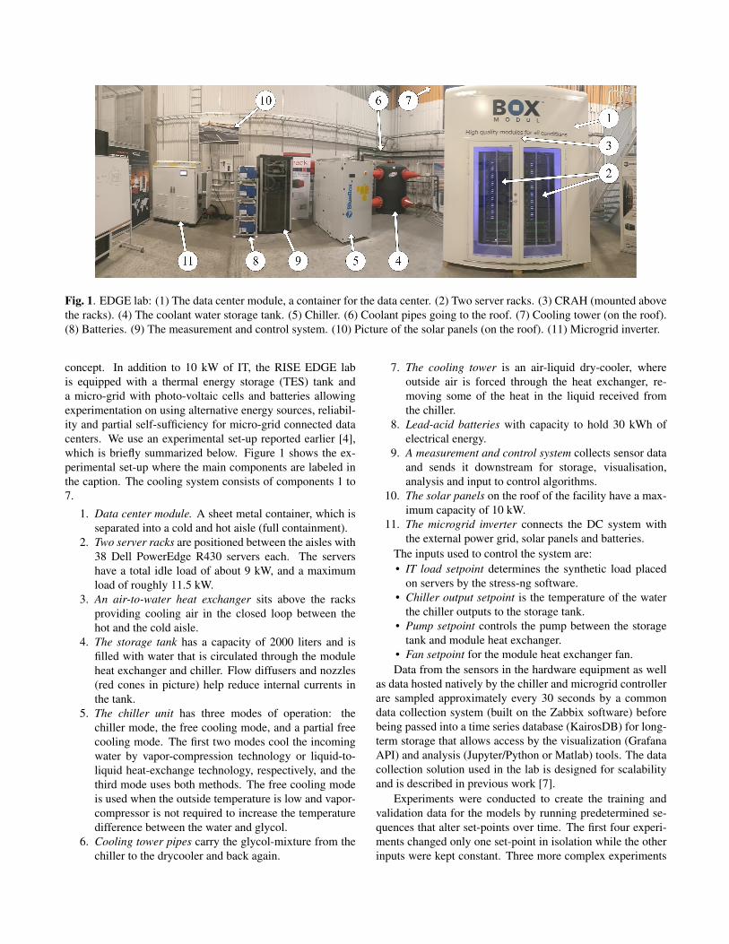
Fig. 1. EDGE lab: (1) The data center module, a container for the data center. (2) Two server racks. (3) CRAH (mounted abovethe racks). (4) The coolant water storage tank. (5) Chiller. (6) Coolant pipes going to the roof. (7) Cooling tower (on the roof).(8) Batteries. (9) The measurement and control system. (10) Picture of the solar panels (on the roof). (11) Microgrid inverter.

concept. In addition to 10 kW of IT, the RISE EDGE labis equipped with a thermal energy storage (TES) tank anda micro-grid with photo-voltaic cells and batteries allowingexperimentation on using alternative energy sources, reliabil-ity and partial self-sufficiency for micro-grid connected datacenters. We use an experimental set-up reported earlier [4],which is briefly summarized below. Figure 1 shows the ex-perimental set-up where the main components are labeled inthe caption. The cooling system consists of components 1 to7.

1. Data center module. A sheet metal container, which isseparated into a cold and hot aisle (full containment).

2. Two server racks are positioned between the aisles with38 Dell PowerEdge R430 servers each. The servershave a total idle load of about 9 kW, and a maximumload of roughly 11.5 kW.

3. An air-to-water heat exchanger sits above the racksproviding cooling air in the closed loop between thehot and the cold aisle.

4. The storage tank has a capacity of 2000 liters and isfilled with water that is circulated through the moduleheat exchanger and chiller. Flow diffusers and nozzles(red cones in picture) help reduce internal currents inthe tank.

5. The chiller unit has three modes of operation: thechiller mode, the free cooling mode, and a partial freecooling mode. The first two modes cool the incomingwater by vapor-compression technology or liquid-to-liquid heat-exchange technology, respectively, and thethird mode uses both methods. The free cooling modeis used when the outside temperature is low and vapor-compressor is not required to increase the temperaturedifference between the water and glycol.

6. Cooling tower pipes carry the glycol-mixture from thechiller to the drycooler and back again.

7. The cooling tower is an air-liquid dry-cooler, whereoutside air is forced through the heat exchanger, re-moving some of the heat in the liquid received fromthe chiller.

8. Lead-acid batteries with capacity to hold 30 kWh ofelectrical energy.

9. A measurement and control system collects sensor dataand sends it downstream for storage, visualisation,analysis and input to control algorithms.

10. The solar panels on the roof of the facility have a max-imum capacity of 10 kW.

11. The microgrid inverter connects the DC system withthe external power grid, solar panels and batteries.

The inputs used to control the system are:• IT load setpoint determines the synthetic load placed

on servers by the stress-ng software.• Chiller output setpoint is the temperature of the water

the chiller outputs to the storage tank.• Pump setpoint controls the pump between the storage

tank and module heat exchanger.• Fan setpoint for the module heat exchanger fan.Data from the sensors in the hardware equipment as well

as data hosted natively by the chiller and microgrid controllerare sampled approximately every 30 seconds by a commondata collection system (built on the Zabbix software) beforebeing passed into a time series database (KairosDB) for long-term storage that allows access by the visualization (GrafanaAPI) and analysis (Jupyter/Python or Matlab) tools. The datacollection solution used in the lab is designed for scalabilityand is described in previous work [7].

Experiments were conducted to create the training andvalidation data for the models by running predetermined se-quences that alter set-points over time. The first four experi-ments changed only one set-point in isolation while the otherinputs were kept constant. Three more complex experiments

FC HEXCRAH

Storagetank

M

M

PrimaryShuntvalve

FCvalve

M

SecondaryShuntvalve

Compressor

Bluebox

Drycooler

User-side pump

Source-side pump

Secondaryuser-side

pump

EvaporatorHEX

CondenserHEX

Expansionvalve

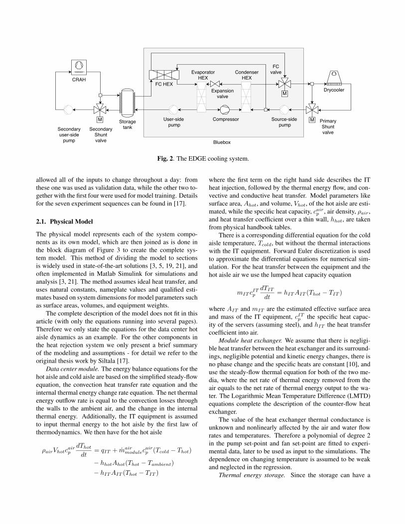
Fig. 2. The EDGE cooling system.

allowed all of the inputs to change throughout a day: fromthese one was used as validation data, while the other two to-gether with the first four were used for model training. Detailsfor the seven experiment sequences can be found in [17].

2.1. Physical Model

The physical model represents each of the system compo-nents as its own model, which are then joined as is done inthe block diagram of Figure 3 to create the complete sys-tem model. This method of dividing the model to sectionsis widely used in state-of-the-art solutions [3, 5, 19, 21], andoften implemented in Matlab Simulink for simulations andanalysis [3, 21]. The method assumes ideal heat transfer, anduses natural constants, nameplate values and qualified esti-mates based on system dimensions for model parameters suchas surface areas, volumes, and equipment weights.

The complete description of the model does not fit in thisarticle (with only the equations running into several pages).Therefore we only state the equations for the data center hotaisle dynamics as an example. For the other components inthe heat rejection system we only present a brief summaryof the modeling and assumptions - for detail we refer to theoriginal thesis work by Siltala [17].

Data center module. The energy balance equations for thehot aisle and cold aisle are based on the simplified steady-flowequation, the convection heat transfer rate equation and theinternal thermal energy change rate equation. The net thermalenergy outflow rate is equal to the convection losses throughthe walls to the ambient air, and the change in the internalthermal energy. Additionally, the IT equipment is assumedto input thermal energy to the hot aisle by the first law ofthermodynamics. We then have for the hot aisle

ρairVhotcairp

dThotdt

= qIT + mairmodulec

airp (Tcold − Thot)

− hhotAhot(Thot − Tambient)

− hITAIT (Thot − TIT )

where the first term on the right hand side describes the ITheat injection, followed by the thermal energy flow, and con-vective and conductive heat transfer. Model parameters likesurface area, Ahot, and volume, Vhot, of the hot aisle are esti-mated, while the specific heat capacity, cairp , air density, ρair,and heat transfer coefficient over a thin wall, hhot, are takenfrom physical handbook tables.

There is a corresponding differential equation for the coldaisle temperature, Tcold, but without the thermal interactionswith the IT equipment. Forward Euler discretization is usedto approximate the differential equations for numerical sim-ulation. For the heat transfer between the equipment and thehot aisle air we use the lumped heat capacity equation

mIT cITp

dTITdt

= hITAIT (Thot − TIT )

where AIT and mIT are the estimated effective surface areaand mass of the IT equipment, cITp the specific heat capac-ity of the servers (assuming steel), and hIT the heat transfercoefficient into air.

Module heat exchanger. We assume that there is negligi-ble heat transfer between the heat exchanger and its surround-ings, negligible potential and kinetic energy changes, there isno phase change and the specific heats are constant [10], anduse the steady-flow thermal equation for both of the two me-dia, where the net rate of thermal energy removed from theair equals to the net rate of thermal energy output to the wa-ter. The Logarithmic Mean Temperature Difference (LMTD)equations complete the description of the counter-flow heatexchanger.

The value of the heat exchanger thermal conductance isunknown and nonlinearly affected by the air and water flowrates and temperatures. Therefore a polynomial of degree 2in the pump set-point and fan set-point are fitted to experi-mental data, later to be used as input to the simulations. Thedependence on changing temperature is assumed to be weakand neglected in the regression.

Thermal energy storage. Since the storage can have a

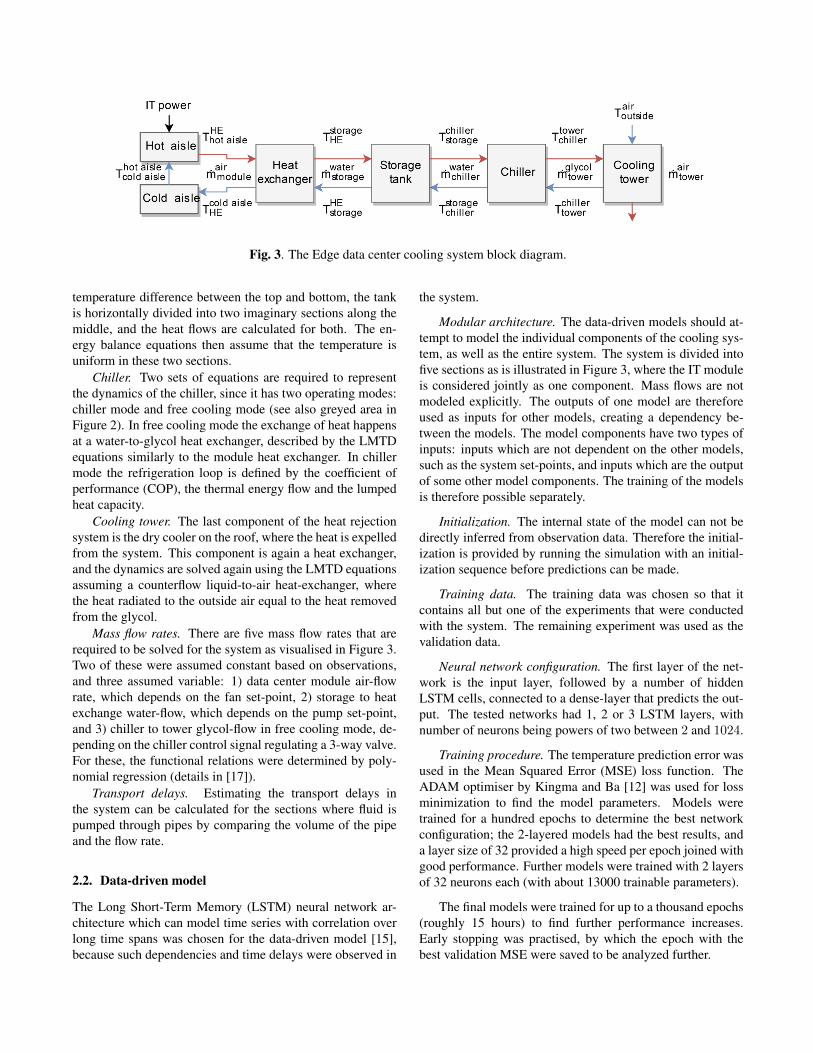
Fig. 3. The Edge data center cooling system block diagram.

temperature difference between the top and bottom, the tankis horizontally divided into two imaginary sections along themiddle, and the heat flows are calculated for both. The en-ergy balance equations then assume that the temperature isuniform in these two sections.

Chiller. Two sets of equations are required to representthe dynamics of the chiller, since it has two operating modes:chiller mode and free cooling mode (see also greyed area inFigure 2). In free cooling mode the exchange of heat happensat a water-to-glycol heat exchanger, described by the LMTDequations similarly to the module heat exchanger. In chillermode the refrigeration loop is defined by the coefficient ofperformance (COP), the thermal energy flow and the lumpedheat capacity.

Cooling tower. The last component of the heat rejectionsystem is the dry cooler on the roof, where the heat is expelledfrom the system. This component is again a heat exchanger,and the dynamics are solved again using the LMTD equationsassuming a counterflow liquid-to-air heat-exchanger, wherethe heat radiated to the outside air equal to the heat removedfrom the glycol.

Mass flow rates. There are five mass flow rates that arerequired to be solved for the system as visualised in Figure 3.Two of these were assumed constant based on observations,and three assumed variable: 1) data center module air-flowrate, which depends on the fan set-point, 2) storage to heatexchange water-flow, which depends on the pump set-point,and 3) chiller to tower glycol-flow in free cooling mode, de-pending on the chiller control signal regulating a 3-way valve.For these, the functional relations were determined by poly-nomial regression (details in [17]).

Transport delays. Estimating the transport delays inthe system can be calculated for the sections where fluid ispumped through pipes by comparing the volume of the pipeand the flow rate.

2.2. Data-driven model

The Long Short-Term Memory (LSTM) neural network ar-chitecture which can model time series with correlation overlong time spans was chosen for the data-driven model [15],because such dependencies and time delays were observed in

the system.

Modular architecture. The data-driven models should at-tempt to model the individual components of the cooling sys-tem, as well as the entire system. The system is divided intofive sections as is illustrated in Figure 3, where the IT moduleis considered jointly as one component. Mass flows are notmodeled explicitly. The outputs of one model are thereforeused as inputs for other models, creating a dependency be-tween the models. The model components have two types ofinputs: inputs which are not dependent on the other models,such as the system set-points, and inputs which are the outputof some other model components. The training of the modelsis therefore possible separately.

Initialization. The internal state of the model can not bedirectly inferred from observation data. Therefore the initial-ization is provided by running the simulation with an initial-ization sequence before predictions can be made.

Training data. The training data was chosen so that itcontains all but one of the experiments that were conductedwith the system. The remaining experiment was used as thevalidation data.

Neural network configuration. The first layer of the net-work is the input layer, followed by a number of hiddenLSTM cells, connected to a dense-layer that predicts the out-put. The tested networks had 1, 2 or 3 LSTM layers, withnumber of neurons being powers of two between 2 and 1024.

Training procedure. The temperature prediction error wasused in the Mean Squared Error (MSE) loss function. TheADAM optimiser by Kingma and Ba [12] was used for lossminimization to find the model parameters. Models weretrained for a hundred epochs to determine the best networkconfiguration; the 2-layered models had the best results, anda layer size of 32 provided a high speed per epoch joined withgood performance. Further models were trained with 2 layersof 32 neurons each (with about 13000 trainable parameters).

The final models were trained for up to a thousand epochs(roughly 15 hours) to find further performance increases.Early stopping was practised, by which the epoch with thebest validation MSE were saved to be analyzed further.

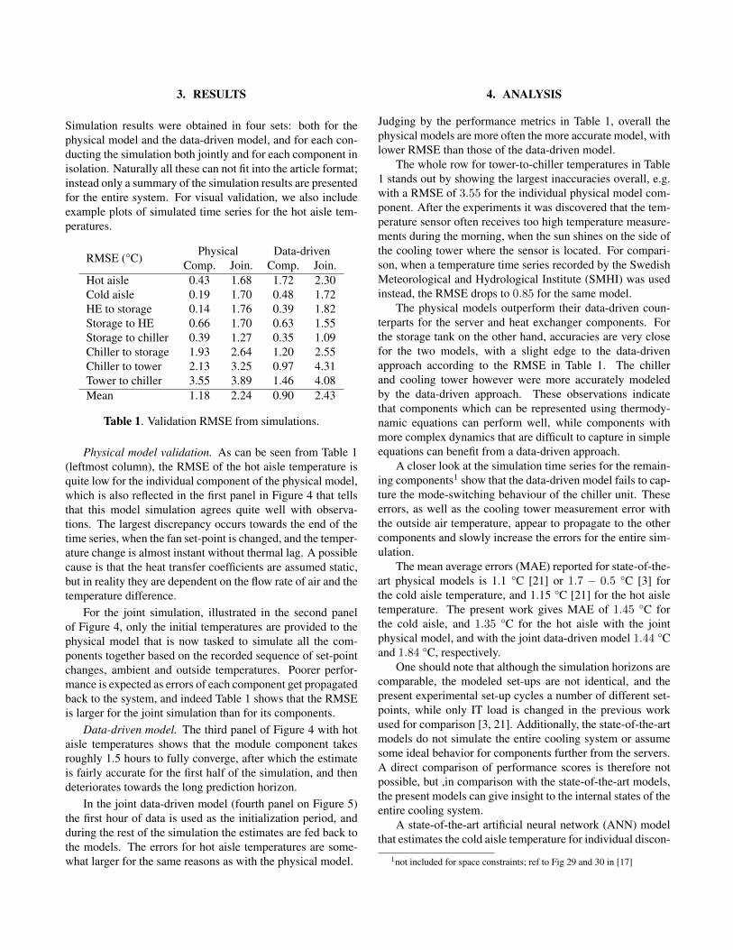
3. RESULTS

Simulation results were obtained in four sets: both for thephysical model and the data-driven model, and for each con-ducting the simulation both jointly and for each component inisolation. Naturally all these can not fit into the article format;instead only a summary of the simulation results are presentedfor the entire system. For visual validation, we also includeexample plots of simulated time series for the hot aisle tem-peratures.

RMSE (°C) Physical Data-drivenComp. Join. Comp. Join.

Hot aisle 0.43 1.68 1.72 2.30Cold aisle 0.19 1.70 0.48 1.72HE to storage 0.14 1.76 0.39 1.82Storage to HE 0.66 1.70 0.63 1.55Storage to chiller 0.39 1.27 0.35 1.09Chiller to storage 1.93 2.64 1.20 2.55Chiller to tower 2.13 3.25 0.97 4.31Tower to chiller 3.55 3.89 1.46 4.08Mean 1.18 2.24 0.90 2.43

Table 1. Validation RMSE from simulations.

Physical model validation. As can be seen from Table 1(leftmost column), the RMSE of the hot aisle temperature isquite low for the individual component of the physical model,which is also reflected in the first panel in Figure 4 that tellsthat this model simulation agrees quite well with observa-tions. The largest discrepancy occurs towards the end of thetime series, when the fan set-point is changed, and the temper-ature change is almost instant without thermal lag. A possiblecause is that the heat transfer coefficients are assumed static,but in reality they are dependent on the flow rate of air and thetemperature difference.

For the joint simulation, illustrated in the second panelof Figure 4, only the initial temperatures are provided to thephysical model that is now tasked to simulate all the com-ponents together based on the recorded sequence of set-pointchanges, ambient and outside temperatures. Poorer perfor-mance is expected as errors of each component get propagatedback to the system, and indeed Table 1 shows that the RMSEis larger for the joint simulation than for its components.

Data-driven model. The third panel of Figure 4 with hotaisle temperatures shows that the module component takesroughly 1.5 hours to fully converge, after which the estimateis fairly accurate for the first half of the simulation, and thendeteriorates towards the long prediction horizon.

In the joint data-driven model (fourth panel on Figure 5)the first hour of data is used as the initialization period, andduring the rest of the simulation the estimates are fed back tothe models. The errors for hot aisle temperatures are some-what larger for the same reasons as with the physical model.

4. ANALYSIS

Judging by the performance metrics in Table 1, overall thephysical models are more often the more accurate model, withlower RMSE than those of the data-driven model.

The whole row for tower-to-chiller temperatures in Table1 stands out by showing the largest inaccuracies overall, e.g.with a RMSE of 3.55 for the individual physical model com-ponent. After the experiments it was discovered that the tem-perature sensor often receives too high temperature measure-ments during the morning, when the sun shines on the side ofthe cooling tower where the sensor is located. For compari-son, when a temperature time series recorded by the SwedishMeteorological and Hydrological Institute (SMHI) was usedinstead, the RMSE drops to 0.85 for the same model.

The physical models outperform their data-driven coun-terparts for the server and heat exchanger components. Forthe storage tank on the other hand, accuracies are very closefor the two models, with a slight edge to the data-drivenapproach according to the RMSE in Table 1. The chillerand cooling tower however were more accurately modeledby the data-driven approach. These observations indicatethat components which can be represented using thermody-namic equations can perform well, while components withmore complex dynamics that are difficult to capture in simpleequations can benefit from a data-driven approach.

A closer look at the simulation time series for the remain-ing components1 show that the data-driven model fails to cap-ture the mode-switching behaviour of the chiller unit. Theseerrors, as well as the cooling tower measurement error withthe outside air temperature, appear to propagate to the othercomponents and slowly increase the errors for the entire sim-ulation.

The mean average errors (MAE) reported for state-of-the-art physical models is 1.1 °C [21] or 1.7 − 0.5 °C [3] forthe cold aisle temperature, and 1.15 °C [21] for the hot aisletemperature. The present work gives MAE of 1.45 °C forthe cold aisle, and 1.35 °C for the hot aisle with the jointphysical model, and with the joint data-driven model 1.44 °Cand 1.84 °C, respectively.

One should note that although the simulation horizons arecomparable, the modeled set-ups are not identical, and thepresent experimental set-up cycles a number of different set-points, while only IT load is changed in the previous workused for comparison [3, 21]. Additionally, the state-of-the-artmodels do not simulate the entire cooling system or assumesome ideal behavior for components further from the servers.A direct comparison of performance scores is therefore notpossible, but ,in comparison with the state-of-the-art models,the present models can give insight to the internal states of theentire cooling system.

A state-of-the-art artificial neural network (ANN) modelthat estimates the cold aisle temperature for individual discon-

1not included for space constraints; ref to Fig 29 and 30 in [17]

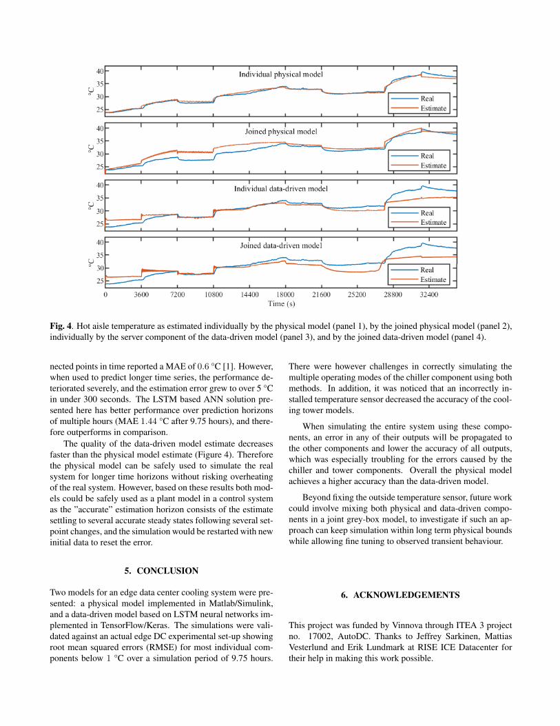
Fig. 4. Hot aisle temperature as estimated individually by the physical model (panel 1), by the joined physical model (panel 2),individually by the server component of the data-driven model (panel 3), and by the joined data-driven model (panel 4).

nected points in time reported a MAE of 0.6 °C [1]. However,when used to predict longer time series, the performance de-teriorated severely, and the estimation error grew to over 5 °Cin under 300 seconds. The LSTM based ANN solution pre-sented here has better performance over prediction horizonsof multiple hours (MAE 1.44 °C after 9.75 hours), and there-fore outperforms in comparison.

The quality of the data-driven model estimate decreasesfaster than the physical model estimate (Figure 4). Thereforethe physical model can be safely used to simulate the realsystem for longer time horizons without risking overheatingof the real system. However, based on these results both mod-els could be safely used as a plant model in a control systemas the ”accurate” estimation horizon consists of the estimatesettling to several accurate steady states following several set-point changes, and the simulation would be restarted with newinitial data to reset the error.

5. CONCLUSION

Two models for an edge data center cooling system were pre-sented: a physical model implemented in Matlab/Simulink,and a data-driven model based on LSTM neural networks im-plemented in TensorFlow/Keras. The simulations were vali-dated against an actual edge DC experimental set-up showingroot mean squared errors (RMSE) for most individual com-ponents below 1 °C over a simulation period of 9.75 hours.

There were however challenges in correctly simulating themultiple operating modes of the chiller component using bothmethods. In addition, it was noticed that an incorrectly in-stalled temperature sensor decreased the accuracy of the cool-ing tower models.

When simulating the entire system using these compo-nents, an error in any of their outputs will be propagated tothe other components and lower the accuracy of all outputs,which was especially troubling for the errors caused by thechiller and tower components. Overall the physical modelachieves a higher accuracy than the data-driven model.

Beyond fixing the outside temperature sensor, future workcould involve mixing both physical and data-driven compo-nents in a joint grey-box model, to investigate if such an ap-proach can keep simulation within long term physical boundswhile allowing fine tuning to observed transient behaviour.

6. ACKNOWLEDGEMENTS

This project was funded by Vinnova through ITEA 3 projectno. 17002, AutoDC. Thanks to Jeffrey Sarkinen, MattiasVesterlund and Erik Lundmark at RISE ICE Datacenter fortheir help in making this work possible.

References[1] J. Athavale, Y. Joshi, and M. Yoda. Artificial neural net-

work based prediction of temperature and flow profilein data centers. In 2018 17th IEEE Intersociety conf onThermal and Thermomechanical Phenomena in Elec-tronic Systems (ITherm), pages 871–880. IEEE, 2018.

[2] Maria Avgerinou, Paolo Bertoldi, and Luca Castellazzi.Trends in data centre energy consumption under the Eu-ropean code of conduct for data centre energy efficiency.Energies, 10(10), 2017.

[3] Y. Berezovskaya, A. Mousavi, V. Vyatkin, andX. Zhang. Smart distribution of IT load in energy ef-ficient data centers with focus on cooling systems. InIECON 2018 - 44th Annual Conference of the IEEE In-dustrial Electronics Society, pages 4907–4912. IEEE,2018.

[4] Rickard Brannvall, Mikko Siltala, Jonas Gustafsson,Jeffrey Sarkinen, Mattias Vesterlund, and Jon Summers.Edge: Microgrid data center with mixed energy storage.In Proceedings of the Eleventh ACM International Con-ference on Future Energy Systems, e-Energy ’20, page466–473, New York, NY, USA, 2020. Association forComputing Machinery. ISBN 9781450380096.

[5] T. J. Breen, E. J. Walsh, J. Punch, A. J. Shah, and C. E.Bash. From chip to cooling tower data center model-ing: Part I Influence of server inlet temperature and tem-perature rise across cabinet. In 2010 12th IEEE Inter-society Conference on Thermal and ThermomechanicalPhenomena in Electronic Systems. IEEE, 2010.

[6] Jim Gao. Machine learning applications for data cen-ter optimization. Google AI Research Publication,2014. [Cited 28.11.2019]. Available at: https://ai.google/research/pubs/pub42542.

[7] Jonas Gustafsson, Sebastian Fredriksson, MagnusNilsson-Maki, Daniel Olsson, Jeffrey Sarkinen, Hen-rik Niska, Nicolas Seyvet, Tor Minde, and JonathanSummers. A demonstration of monitoring and measur-ing data centers for energy efficiency using opensourcetools. pages 506–512, 06 2018.

[8] B. Hadid, S. Lecoeuche, D. Gille, and C. Labarre. En-ergy efficiency of data centers: A data-driven model-based approach. In 2016 IEEE International EnergyConference (ENERGYCON). IEEE, 2016.

[9] C.M. Healey, J.W. VanGilder, M. Condor, and W. Tian.Transient data center temperatures after a primary poweroutage. pages 865–870, 2018.

[10] Frank P. Incropera, David P. DeWitt, Theodore L.Bergman, and Adrienne S. Lavine. Principles of Heat

and Mass Transfer; International Student Version. Wi-ley, 7th edition, 2013.

[11] M. Iyengar, H. Hamann, R. R. Schmidt, andJ. Vangilder. Comparison between numerical and exper-imental temperature distributions in a small data centertest cell. In 2007 Proceedings of the ASME InterPackConference, IPACK 2007, volume 1, pages 819–826,2007.

[12] Diederik P. Kingma and Jimmy Ba. Adam: A methodfor stochastic optimization. In ICLR, 2015. URLhttp://arxiv.org/abs/1412.6980.

[13] Jonathan G. Koomey. Growth in data center elec-tricity use 2005 to 2010. Technical report, AnalyticsPress, 2011. [Cited 6.12.2019]. Available at: https://www.koomey.com/research.html.

[14] R. Lucchese and A. Johansson. On energy efficient flowprovisioning in air-cooled data servers. Control Engi-neering Practice, 89:103–112, 2019.

[15] J. Schmidhuber. Deep learning in neural networks: Anoverview. Neural Networks, 61:85–117, 2015.

[16] H. Shoukourian, T. Wilde, D. Labrenz, and A. Bode. Us-ing machine learning for data center cooling infrastruc-ture efficiency prediction. In 2017 IEEE InternationalParallel and Distributed Processing Symposium Work-shops (IPDPSW), pages 954–963. IEEE, 2017.

[17] Mikko Siltala. Simulating data center cooling systems:data-driven and physical modeling methods. Master’sthesis, Aalto University, 2020.

[18] James W. VanGilder, Christopher M. Healey, MichaelCondor, Wei Tian, and Quentin Menusier. A compactcooling-system model for transient data center simula-tions. In 2018 17th IEEE Intersociety Conference onThermal and Thermomechanical Phenomena in Elec-tronic Systems (ITherm). IEEE, may 2018.

[19] E. J. Walsh, T. J. Breen, J. Punch, A. J. Shah, and C. E.Bash. From chip to cooling tower data center modeling:Part II Influence of chip temperature control philosophy.In 2010 12th IEEE Intersociety Conference on Thermaland Thermomechanical Phenomena in Electronic Sys-tems. IEEE, June 2010.

[20] E Wibron, Anna-Lena Ljung, and T Lundstrom. Com-putational fluid dynamics modeling and validating ex-periments of airflow in a data center. Energies, 11, 022018.

[21] G. Zhabelova, M. Vesterlund, S. Eschmann, Y. Bere-zovskaya, V. Vyatkin, and D. Flieller. A comprehensivemodel of data center: From CPU to cooling tower. IEEEAccess, 6:61254–61266, 2018.