SILCA: Fast-Yet-Accurate Time-Domain Simulation of VLSI Circuits with Strong Parasitic Coupling Effects*

Zhao Li and C.-J. Richard Shi Department of Electrical Engineering, University of Washington

Seattle, WA 98195 lz2000, cjshi@ee.washington.edu

Abstract: We propose a new circuit analysis method, namely Semi-Implicit Linear-Centric Analysis (SILCA), for efficient SPICE-accurate transient simulation of deep-submicron VLSI circuits with strong parasitic coupling effects introduced by interconnect lines, common substrate, power/ground networks, etc. SILCA is based on two linear-centric techniques. First, a new semi-implicit iterative numerical integration scheme is developed, which applies dynamic time step control accounting for stiff systems and meanwhile keeps constant equivalent conductance for capacitor/inductor companion models. Its convergence and stability properties are characterized. Second, to achieve constant linearized conductance for nonlinear devices during nonlinear iteration process, a successive variable chord method is introduced as an alternative of the Newton-Raphson method and the rank-one update technique is implemented for fast LU factorization. With these techniques, SILCA reduces the number and cost of required LU factorizations dramatically. Experimental results on substrate and power/ground networks have demonstrated that SILCA yields SPICE-like accuracy with an over 80X reduction in LU factorization cost, and an about 20X overall CPU time speedup over SPICE3 for circuits with tens of thousands elements, and the efficiency increases further with the size of a circuit. 1. Introduction

With the increasing operation frequency, lower supply voltage and smaller device feature size, parasitic coupling effects are becoming more and more important in modern deep-submicron VLSI circuit designs [1]. The increasing demand to integrate digital, analog and radio frequency (RF) circuits into one single chip requires accurate analysis of VLSI circuits together with surrounding environments, such as interconnect lines, common substrate, power/ground networks, on-chip and packaging inductance, etc. [1][2][3][4][14]. For such purpose, as well as high fidelity coupled circuit and electromagnetic modeling [16], SPICE-like simulators are desirable for accurate transistor-level time-domain simulation.

However, efficient simulation of such systems presents a complexity challenge to SPICE [5]. To accomplish transient simulation, SPICE uses numerical integration formulae [6][7] to form companion models for capacitors and inductors at each time point, and applies the Newton-Raphson (NR) method [6] to linearize nonlinear devices. Then the circuit system is simulated at each time point by iteratively solving a system of linear equations Ax = b, where A is typically a so-called modified nodal analysis (MNA) circuit matrix [5][6]. For strongly coupled systems, the per-

* This research was supported by DARPA NeoCAD Program under Grant

No. N66001-01-8920 and NSF CAREER Award under Grant No. 9985507.

iteration cost of transient simulation with SPICE is dominated by LU factorization [6] of circuit matrix A. The practical cost for LU factorization by using sparse matrix solvers [8] is O(n1.1~1.5) for sparse circuits, where n is the circuit matrix size. However, considering strong coupling effects present in deep sub-micron circuits, since the circuit matrix can become much denser, even with model order reduction [10], the cost for LU factorization can approach its worst case O(n3) [1].

A key idea to improve the efficiency of SPICE-accurate simulation of a large-scale circuit with strong parasitic coupling is to develop innovative simulation approaches to decrease the number of LU factorizations required for the entire time-domain simulation [17][18]. Recently [9] proposes to perform time-domain simulation by using a single fixed time step and the successive chord (SC) method [6] for linearlizing nonlinear devices. Since the MNA circuit matrix for a fixed time step and a fixed chord will not change during transient simulation, only one LU factorization is required. Coupled with model order reduction and table lookup MOSFET models, this idea has been demonstrated to be effective for the simulation of single-stage digital logic gates driving large-size parasitic networks [9]. Unfortunately, there are two principal difficulties that restrict the use of this linear-centric idea successfully to the simulation of general VLSI circuits: 1) Most VLSI circuits have widely distributed time constants, and require dynamic time step control for the simulation efficiency and accuracy. With varying time steps, the circuit matrix is no longer constant for every time point. 2) The SC method has the linear convergence rate. It often needs excessive amount of iterations to converge, and thus requires a huge number of forward/backward substitutions (FBSs) [6].

This paper presents SILCA Semi-Implicit Linear Centric Analysis a new method capable of analyzing VLSI circuits containing strong parasitic couplings with SPICE-like accuracy yet orders of magnitude speedup. SILCA consists of two new ideas that can help keep the MNA matrix as constant as possible during transient simulation even with varying time steps: 1) Semi-implicit iterative integration scheme to keep equivalent

conductance of capacitor/inductor companion models constant for a relatively large time interval;

2) Successive variable chord (SVC) method to keep linearized conductance of nonlinear devices constant for a relatively large voltage/current range. Rank-one update technique is further applied for fast LU factorization.

With these, the required LU factorizations can be reduced by orders of magnitude with a small increase of iterations. Further, the entire method is stable, accurate, and has been implemented to SPICE3.

This paper is organized as follows. Section 2 proposes the new semi-implicit iterative integration scheme. The SVC method and rank-one update technique are presented in Section 3. Section 4 describes the SILCA algorithm. Experimental results on substrate

793

Permission to make digital or hard copies of all or part of this work forpersonal or classroom use is granted without fee provided that copies arenot made or distributed for profit or commercial advantage and thatcopies bear this notice and the full citation on the first page. To copyotherwise, to republish, to post on servers or to redistribute to lists,requires prior specific permission and/or a fee. ICCAD’03, November 11-13, 2003, San Jose, California, USA. Copyright 2003 ACM 1-58113-762-1/03/0011 ...$5.00.

and power/ground coupling analysis are shown in Section 5. Finally, Section 6 concludes this paper.

where z = -h/(2τ) and τ is the time constant of a circuit. From Theorem 2, several observations can be made on the

stability: 1) The semi-implicit TR formula is not A-stable [6] when α >1 since the absolute stability region will approach that of the FE formula, so it cannot be used as a dynamic time step control scheme independently. 2) When α < 1, the semi-implicit TR formula is A-stable. Thus SILCA implements the semi-implicit TR formula as a predictor when α < 1 to provide a good initial guess for the present simulation time point. 3) The semi-implicit TR formula has the “stiff decay” [7] property when α < 1. It means that a decent description of the solution in rapidly switching moments could be maintained in the highly stiff case, whereas the standard TR formula generally encounters numerical oscillation phenomena.

2. Semi-implicit iterative integration scheme

To implement the linear-centric idea for time-domain simulation, we propose a new semi-implicit iterative integration scheme. First, semi-implicit integration formulae are used as a predictor to provide a good initial guess for the present time point. Second, iterative integration formulae are applied as a corrector to achieve the final accurate solution and to ensure numerical stability at the same time. Both of the new integration formulae will keep the equivalent conductance of capacitor/inductor companion models constant for a relatively larger time interval.

2.1 Semi-implicit integration predictor 2.2 Iterative integration corrector In [1], semi-implicit integration scheme has been suggested for

strongly coupled interconnect systems. In this sub-section, we extend this idea and introduce a generalized semi-implicit integration predictor for dynamic step transient simulation.

The LTE and stability problems of the semi-implicit integration formulae come from the approximation step with explicit integration formulae in Eq. (1). In this section, we further propose an improvement of this scheme by using iteration.

Let h be a basis time step size. The time step size hn for the present time point tn can be represented by hn = αh, where α is a positive scalar. Now let us rearrange the standard trapezoid (TR) formula as follows:

Rather than using explicit integration formulae, the xn in the third term of Eq. (3) is replaced by the (k-1)-th iteration solution

at the present time point and a new k-th iteration

solution is achieved by solving Eq. (3), where k is the iteration number. This leads to the iterative version of Eq. (3), called the constant-conductance iterative trapezoid formula, written as follows:

)1( −knx

)(knx

111

1111

)()1(222

)(2)(2

−

•

−−

−

•

−−

•

−

•

−−−

−−=

−−=−−=

nnnnn

nnnnnnn

n

xxxh

xh

xh

xxxh

xxxh

x

αα

α

•

(1)

11

)1()1()(

11)1(

1)()(

222

)()1(222

−

•−

−−

−

•

−−

−

•

−−

+−=

−−−

−−=

nn

knk

nk

n

nnk

nnk

nk

n

xh

xxx

hx

h

xxxh

xh

xh

x

α

αα

)(k )1( −k

(4)

where xn = x(tn), xn-1 = x(tn-1), tn = tn-1 + αh, x and are first-order time derivatives at t

n 1−

•

nxn and tn-1, respectively. Noting that the

first term leads to the constant equivalent conductance, we would like to represent the xn in the third term by all the known values from the previous time points. This can be done using any explicit Adams-Bashforth formula [6]. The simplest is the forward Euler (FE) formula with step size αh as follows:

where and are the solution of the present time point for iteration k and k-1 respectively. If the iterative integration formulae converge successfully, the LTE requirement will be satisfied since the final converged solution is the same as that with the implicit integration formulae.

nx nx

11 −

•

− += nnn xhxx α (2) Then the following constant-conductance semi-implicit trapezoid integration formula for step size αh is derived:

To study the convergence property, let us re-write the circuit equation as below:

11 )12(22−

•

−

•

−−−= nnnn xxh

xh

x α (3) bxCGx =+•

where G and C represent the conductance and susceptance matrices, and b is the vector of input sources. Replace time derivatives by the iterative trapezoid formula Eq. (4), we have

When α = 1, the above formula reduces to the standard TR formula. When α = 1/2, it represents the backward Euler (BE) formula with step size h/2. We can formally prove the following theorem:

bxCxCxCxCG

bxxx

xxCGx

nnk

nk

n

nn

knk

nk

nk

n

+++

−=

+

=

−

−+−+

−

•

−−

−

•−

−−

11)1()(

11

)1()1()()(

22112

222

hhh

hhh

αα

α Theorem 1: The local truncation error ε of the constant-conductance semi-implicit trapezoid formula with time step size αh is given by (xξ= x(tξ), tξ is between tn-1 and tn)

( ) ( )32

65.11

211 h

xh

xα

αα

αε ξξ

−+

−=

•••••

Clearly the iterative trapezoid formula converges if

12112 1

<

−

+

−

hhCCG

α

The proof is a straightforward application of the local truncation error (LTE) estimation for the standard TR formula [6]. where ||•|| represents the special radius of the iteration matrix. In the

worst case (G is zero), to achieve convergence, 0.5<α<∞ is required. In practice, to speed up the convergence and ensure accuracy, 0.625<α <2.5 is used.

The stability property of the semi-implicit TR formula can be proved as below: Theorem 2: The absolute stability region of the constant-conductance semi-implicit trapezoidal formula with time step size αh is defined by

The absolute stability regions of iterative integration formulae are also related to the iteration number k. We can formally prove the following Theorem 3: 1

1)12(1

<−

−+z

zα

794

Figure 1. Absolute stability region of the iterative TR formula for

α=0.625 and k=2.

Figure 2. Absolute stability region of the iterative TR formula for

α=2.5 and k=2.

Theorem 3: The absolute stability region of the constant-conductance iterative trapezoidal formula for step size αh is defined by

1/1/1)

/12()

1/11( <

−+

+−−

−zz

zz

zk

αα

αα

where z = -h/(2τ) and τ is the time constant for a circuit. The absolute stability regions for α = 0.625 and α = 2.5 when k = 2 are shown in Fig. 1 and Fig. 2, respectively, which satisfy the “stiff stability” requirements suggested by Gear [11]. Furthermore, if 0.5<α<∞ (as required by the convergence property), the absolute stability region will finally reach that of the standard TR formula when k→∞. Therefore, the iterative integration formulae can be applied to either decaying or oscillating systems. In practice, to ensure A-stability, a lower time step size limit could be set so that the standard TR formula is applied under the condition that the present time step is less than the lower limit.

+Vout1

-

+-

1H

1F 1F

1Ω

0.1F0.1F

0.1H 0.1Ω

+Vout2

-

Figure 3. A linear RCL circuit example.

The efficiency of the semi-implicit iterative integration scheme can be illustrated with a simple linear circuit example shown in Fig. 3. It includes two RCL filters with time constants that differ by a

factor of 100. The input is a pulse signal (initially in the low voltage level 0v) with 50% duty ratio and 80 sec period. The simulation length is set to 160 sec. Since the minimum time constant is 0.01 sec, at least 16000 time points are required for a fixed-step transient simulation. Simulation results with SILCA and SPICE3 are shown in Table I, where #Total points represents the number of total simulated time points and #Accepted points represents the number of actual accepted time points. It can be seen in Table I that SILCA and SPICE3 achieve similar #Total points and #Accepted points, which are much less than that required by a fixed step method. Furthermore, the number of LUs with SILCA is decreased to 1.14% of that with SPICE3 (or 87.63X LU reduction). The number of iterations has been increased to about 2.5X.

Table I. Simulation results for a linear RCL circuit example. # Total

points # Accepted

points # Iteration # LU

SPICE3 2630 1965 5258 5258 SILCA 2636 1971 12649 60

Figure 4. Distribution of actual time step sizes and time-domain output

waveform of Vout1.

Figure 5. Distribution of basis time step sizes.

Figure 4 shows the distribution of actual simulated time step sizes (αh) and the output waveform of Vout1. The distribution of simulated time step sizes is much denser when Vout1 is close to 0v. The reason is that the relative LTE for a low voltage level is small, so time step sizes are restricted by the relative LTE and cannot change too much when Vout1 is close to 0v. It can be seen that most of simulated time step sizes are between 0.05 sec and 0.2 sec, centering around 0.08 sec. Recall that the iterative integration

795

formulae can make a relaxation of 0.625<α <2.5, it is possible that only a few basis time step sizes are required for MNA stamping. Figure 5 shows the distribution of basis time step sizes (h) used for MNA stamping during SILCA simulation. It can be seen that the circuit matrix is now kept constant for a larger time interval (i.e., between 45 sec and 80 sec). 3. Successive variable chord method

In SPICE, a new LU factorization is required for each Newton-Raphson iteration. This can be extremely costly for a circuit system with strong parasitic coupling effects. The successive chord method [6] always uses a fixed chord as the first order dI/dV derivative during nonlinear iteration. Hence, at each time point, only one LU factorization is needed for nonlinear iteration. But it is generally difficult to choose a single fixed chord for a (strongly) nonlinear curve to always ensure a good convergence rate.

To achieve a good balance between the number of LUs and that of iterations, we propose to use the successive variable chord (SVC) method. The basic idea is to split a nonlinear curve into different segments, each of which represents a weakly nonlinear curve and the same (local) chord is used for the same segment during nonlinear iteration – so-called Piecewise Weakly Nonlinear (PWNL) analysis. As shown in Fig. 6, the nonlinear curve is divided into three PWNL segments with three local chords defined respectively. A new LU factorization is performed only if the nonlinear curve enters a different PWNL segment with the local chord varied.

I

V0

PWNL#1

PWNL#2

PWNL#3

Chord#1

Chord#2

Chord#3

Figure 6. A PWNL example implemented with the SVC method.

The PWNL idea implemented with the SVC method is in practice very effective due to the following facts: 1) MOSFETs in analog applications generally operate linearly around their operating points, only weakly nonlinearity properties may be present. A fixed chord representing the gm, gmbs, and gds of MOSFETs at operating points is generally good enough. 2) MOSFETs in digital applications reside in two regions most of the time – cutoff region and well-conducted linear region with a very small source-to-drain voltage, both regions have a relatively steady gm, gmbs, and gds. The only situation where gm, gmbs, and gds change a lot is the time when MOSFETs switch from the cut-off region through the saturation region to the linear region (or vice versa), which only occupies a small fraction of total simulation time for a MOSFET in a large digital system. So, a fixed chord for these situations will not significantly affect the total iteration process.

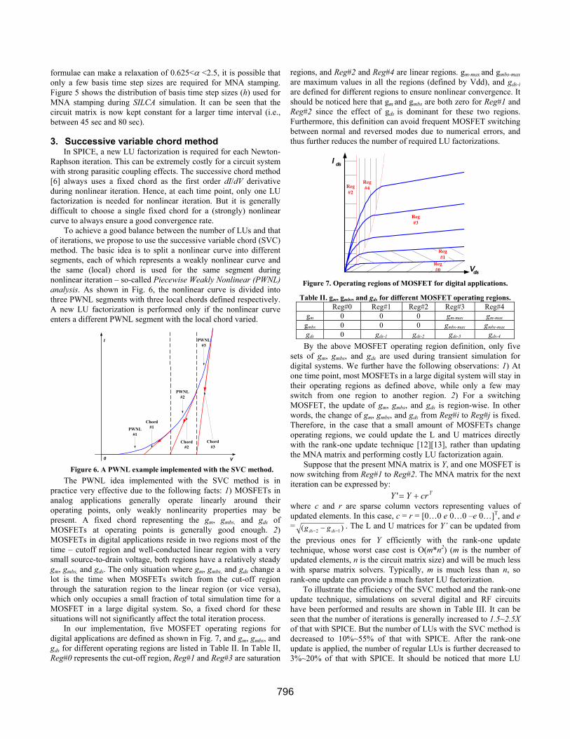
In our implementation, five MOSFET operating regions for digital applications are defined as shown in Fig. 7, and gm, gmbs, and gds for different operating regions are listed in Table II. In Table II, Reg#0 represents the cut-off region, Reg#1 and Reg#3 are saturation

regions, and Reg#2 and Reg#4 are linear regions. gm-max and gmbs-max are maximum values in all the regions (defined by Vdd), and gds-i are defined for different regions to ensure nonlinear convergence. It should be noticed here that gm and gmbs are both zero for Reg#1 and Reg#2 since the effect of gds is dominant for these two regions. Furthermore, this definition can avoid frequent MOSFET switching between normal and reversed modes due to numerical errors, and thus further reduces the number of required LU factorizations.

I ds

Vds

Reg#2

Reg#3

Reg#4

Reg#1

Reg#0

Figure 7. Operating regions of MOSFET for digital applications.

Table II. gm, gmbs, and gds for different MOSFET operating regions. Reg#0 Reg#1 Reg#2 Reg#3 Reg#4

gm 0 0 0 gm-max gm-max gmbs 0 0 0 gmbs-max gmbs-max gds 0 gds-1 gds-2 gds-3 gds-4

By the above MOSFET operating region definition, only five sets of gm, gmbs, and gds are used during transient simulation for digital systems. We further have the following observations: 1) At one time point, most MOSFETs in a large digital system will stay in their operating regions as defined above, while only a few may switch from one region to another region. 2) For a switching MOSFET, the update of gm, gmbs, and gds is region-wise. In other words, the change of gm, gmbs, and gds from Reg#i to Reg#j is fixed. Therefore, in the case that a small amount of MOSFETs change operating regions, we could update the L and U matrices directly with the rank-one update technique [12][13], rather than updating the MNA matrix and performing costly LU factorization again.

Suppose that the present MNA matrix is Y, and one MOSFET is now switching from Reg#1 to Reg#2. The MNA matrix for the next iteration can be expressed by:

TcrYY +=' where c and r are sparse column vectors representing values of updated elements. In this case, c = r = [0…0 e 0…0 –e 0…]T, and e = )( 12 −− − dsds gg . The L and U matrices for Y’ can be updated from

the previous ones for Y efficiently with the rank-one update technique, whose worst case cost is O(m*n2) (m is the number of updated elements, n is the circuit matrix size) and will be much less with sparse matrix solvers. Typically, m is much less than n, so rank-one update can provide a much faster LU factorization.

To illustrate the efficiency of the SVC method and the rank-one update technique, simulations on several digital and RF circuits have been performed and results are shown in Table III. It can be seen that the number of iterations is generally increased to 1.5~2.5X of that with SPICE. But the number of LUs with the SVC method is decreased to 10%~55% of that with SPICE. After the rank-one update is applied, the number of regular LUs is further decreased to 3%~20% of that with SPICE. It should be noticed that more LU

796

speed-up with rank-one update is achieved for relatively large systems, such as a 20-stage inverter chain, a ring oscillator and a VCO. Very little benefit can be achieved on simple systems, such as a single inverter, a single NAND2 gate, etc. Rank-one update technique will be very efficient for a nonlinear system with strong parasitic coupling effects, since only the L and U matrices for the sparse nonlinear part need to be updated during nonlinear iteration, and the dense linear part remains unchanged.

5. Experimental results 5.1 Substrate coupling example

Table III. Simulation results on test circuits. # LU

Test Circuits #Total points

#Acceptpoints

#Iter w/o rnk1

w rnk1

142 127 351 351 - Inv 145 129 545 73 65 369 266 1201 1201 - 20-stage inverter

chain 358 260 2401 493 66 132 123 313 313 - Nand2 123 114 541 73 60 501 421 1542 1542 - One-shot trigger 486 421 3595 438 213 145 127 455 455 - Comparator 148 130 1131 130 66 243 173 1031 1031 - Ring Oscillator 257 178 2420 571 30

1506 1045 7630 7630 - VCO 1468 1042 16146 739 221

The first example is a simple substrate coupling network as shown in Fig. 8. It includes two inverters with pulse inputs in different operating frequencies – the first inverter operates at a low frequency and the second inverter operates at a high frequency. The bulk contacts of nMOSFETs are directly connected to P-substrate ports, and those of pMOSFETs are connected to P-substrate ports through a capacitor between the N-well and the P-substrate [2]. There are four other P-substrate ports connecting to the ground and the backplane of the substrate is also connected to the ground. RCL loads are added at the output of each inverter (not shown in Fig. 8. The substrate is modeled as a dense resistor network [14] that is formed by a 3-dimensional dense resistor mesh with multiple layers; In Fig. 8, a one-layer resistor network is illustrated to model the substrate among four inverter bulk contacts.

+-

+Vout1

-10µ/1µ

25µ/1µ

+Vin1

-

+-

+Vout2

-10µ/1µ

25µ/1µ

+Vin2

-

Cwell 1 Cwell 2

Port

*Note: For each circuit, the 1st row is the SPICE3 result, the 2nd row is the SILCA result

4. The SILCA algorithm

Table IV. Transient simulation flow in SILCA. DC operating point analysis Choose an initial step size h0, the basis step size h = h0, t = 0 WHILE (t<Tfinal)

OUTER LOOP: do α = hn/h, iter_no = 0 INNER LOOP: do

IF(0.625<α<2.5) IF(α<1 && iter_no==0)

Apply Semi-Implicit Integration Predictor Eq. (3) Apply Iterative Integration Corrector Eq. (4)

ELSE IF(iter_no==0) h = hn Apply Standard Implicit Integration Scheme

Apply the SVC method on nonlinear devices IF (0.625<α<2.5)

IF (chord is changed) Apply Rank-one update & FBS ELSE Apply FBS

ELSE Apply LU factorization & FBS iter_no = iter_no + 1

while (not converged) Choose a new hn based on LTE requirement

while (LTE greater than predefined error limit) t = t + hn

Figure 8. The substrate coupling example. Although simplified truncated substrate models have been

proposed to capture dominant coupling conductance [2][14], they are likely to underestimate coupling effects in circuit systems designed to be noise mature [1]. Furthermore, the accuracy with simplified substrate models may not be sufficient. Therefore, accurate analysis of a circuit with a fully modeled substrate is desirable for high fidelity circuit design and verification.

Figure 9. Transient output waveform of the first inverter for the

substrate coupling example. The basic flow for SILCA transient simulation is shown in Table IV. Practical considerations, such as breakpoints [5], are not included in this flow for clarity. In this flow, a new LU factorization is only required when standard implicit integration scheme is used. In case that only local chords of nonlinear devices change, rank-one update is performed for fast LU factorization. No LU factorization is needed in any other case.

Figure 9 shows the transient output waveform of the first inverter when the output signal is digital “1” (the high voltage level). First, the result from SILCA matches that from SPICE3. Second, it can be seen that high frequency feed-through signals from the second inverter are present in Fig. 9. This is an important first-pass design failure reason in deep-submicron digital and

797

analog circuit designs, which may often not be captured by simplified substrate analysis [2][3].

Table V is the statistics of running SILCA on a number of substrate analysis examples with varying circuit substrate network complexity. In our experiments, the number of layers and the number of resistors per layer are changed to vary the total number of circuit elements. A maximum 40.25X LU speed-up and 17.32X overall speed-up (with about 35 thousand elements) are achieved for this simple substrate coupling analysis example, and the FBS cost is increased to 2.5~3X.

Several observations are: 1) The larger the LU/FBS cost ratio are, the more overall speed-up can be achieved with SILCA. Therefore, SILCA is very suitable for deep-submicron circuit systems with strong parasitic coupling effects; 2) Device load cost with SILCA is decreased, which is proportional to the LU speed-up, since device load of resistors are only required when a new LU is performed. 3) The maximum overall speed-up will reach the LU speed-up (around 30X for this example) for large strongly coupled systems. Figure 10 shows the run time comparison between SILCA and SPICE3 with the number of total circuit elements varied. No

rank-one update technique is used for the substrate coupling example.

Figure 10. Run time comparison of the substrate coupling example.

Table V. Simulation results for the substrate coupling analysis example.

SPICE3 SILCA Speed-up #Layer x #Res_Per_Layer #Elements

LU (sec) FBS (sec) Load(sec) LU/FBS LU(sec) FBS(sec) Load(sec) LU Overall

1x1281 1281 32.96 3.99 8.68 8.26 0.96 11.87 1.18 34.33 3.26

2x1281 2562 249.29 14.24 22.56 17.51 9.73 39.80 1.99 25.62 5.55

3x1281 3886 663.86 23.19 35.78 28.63 16.49 63.32 2.40 40.25 8.79

4x1281 5124 2.533e3 59.26 91.77 42.75 78.91 147.27 4.66 32.10 11.63

5x1281 6405 4.496e3 88.37 123.87 50.87 131.22 249.40 7.79 34.26 12.12

6x4961 29766 2.455e5 2.947e3 2.927e3 83.32 8.297e3 7.722e3 112.37 29.59 15.58

7x4961 34727 5.348e5 5.629e3 5.318e3 95.00 1.770e4 1.361e4 195.06 30.21 17.32

5.2 Power/ground analysis example

Vin

. . . . . . . . . . . .

. . . . . . . . . . . .

. . . . . . . . . . . .

. . . . . . . . . . . .

. . . . . . . . . . . .

. . . . . . . . . . . .

Vdd

Vdd

Vdd

Vdd

. . . . . . . . . . . .. . . . . . Vout

Figure 11. The power/ground analysis example.

The second example is a power/ground network as shown in Fig. 11. The power and ground supply networks are modeled as two RCL mesh layers (parasitic coupling capacitors are not shown in Fig. 11). For fast transient simulation of a nonlinear circuit with power/ground networks, nonlinear devices are generally simplified as (piecewise linear) current sources plus device parasitic capacitors [4][15], to model real nonlinear device behaviors. However, this is generally hard and not accurate for a

large circuit. Accurate simulation of a full-scale power/ground network is highly desirable for accurate circuit verification and power/ground optimization. In our example, between these two layers is a 20-stage inverter chain, different inverters of which are connected to different power/ground nodes. Furthermore, RCL loads are added for each inverter to model interconnect lines between adjacent stages.

Figure 12. Transient output waveform of the inverter chain for

power/ground analysis example. Figure 12 shows the transient output waveform of the inverter

chain when the output signal is digital “1” (the high voltage level).

798

The “1” signal has been disturbed due to the IR-drop (the input Vdd is 3.3v) and L*dI/dt effects of the power/ground network. Table VI shows the simulation results with varied numbers of elements modeling the power/ground network. In our experiments, the size of two RCL meshes is changed to vary the number of elements. We can see that SILCA achieves more speed-up for larger circuits. It is worthy to notice that, the maximum LU speed-up and overall speed-up reach 87.70X and 18.97X (with about 60 thousand elements) respectively with the rank-one update technique, which are 24.88X and 11.86X, respectively, with only the SVC method. 6. Conclusions

In this paper, a new time-domain nonlinear circuit simulation method called SILCA has been proposed for deep-submicron VLSI circuit design and verification, where requires accurate modeling of parasitic couplings or coupled circuit and electromagnetic modeling. A new dynamic time-step semi-implicit iterative numerical integration scheme was developed to keep constant equivalent conductance for capacitor/inductor companion models. We also proved the convergence and stability property of the new introduced integration formulae. A successive variable chord method was further proposed as an alternative of the Newton-Raphson method and the rank-one update technique has been implemented for fast LU factorization. With these techniques, SILCA can reduce the number of costly LU factorization dramatically in transient simulation. Experimental results on substrate and power/ground networks have demonstrated that SILCA yields SPICE-like accuracy with orders of magnitude speed-up over SPICE3. 7. References [1] J. R. Phillips and L. M. Silveira, “Simulation Approaches for

Strongly Coupled Interconnect Systems”, Proc. IEEE/ACM Int. Conf. on Computer-Aided Design, pp. 430-437, November 2001.

[2] A. Samavedam, A. Sadate, K. Mayaram, and T. S. Fiez, “A Scalable Substrate Noise Coupling Model for Design of Mixed-Signal IC’s”, IEEE Journal of Solid-State Circuits, vol. 35, no. 6, pp. 895-904, June 2000.

[3] M. Nagata, J. Nagai, K. Hijikata, T. Morie, and A. Iwata, “Physical Design Guides for Substrate Noise Reduction in CMOS Digital Circuits”, IEEE Journal of Solid-State Circuits, vol. 36, No. 3, pp. 539-549, March 2001.

[4] H. Su, K. H. Gala and S. S. Sapatnekar, “Fast Analysis and Optimization of Power/Ground networks”, Proc. IEEE/ACM Int. Conf. on Computer-Aided Design, pp. 477-480, November 2000.

[5] L. W. Nagel, SPICE: A Computer Program to Simulate Semiconductor Circuits, University of California, Berkeley, Tech. Rep., UCB/ERL M520, May 1975.

[6] W. J. McCalla, Fundamentals of Computer-Aided Circuit Simulation, Kluwer Academic Publishers, 1988.

[7] U. M. Ascher and L. R. Petzold, Computer Methods for Ordinary Differential Equations and Differential-Algebraic Equations, SIAM, 1998.

[8] K. S. Kundert and A. Sangiovanni-Vincentelli, Sparse User’s Guide – A Sparse Linear Equation Solver Version 1.3a, University of California, Berkeley, April 1988.

[9] E. Acar, F. Dartu, and L. T. Pileggi, “TETA: Transistor-Level Waveform Evaluation for Timing Analysis”, IEEE Trans. on Computer-Aided Design, vol. 21, no. 5, pp. 605-616, May 2002.

[10] A. Odabasioglu, M. Celik, and L. T. Pillegi, “PRIMA: Passive Reduced-Order Interconnect Macromodeling Algorithm”, IEEE Trans. on Computer-Aided Design, vol. 17, no. 8, pp. 645-654, August 1998.

[11] C. W. Gear, Numerical Initial Values Problems in Ordinary Differential Equations, Prentice-Hall, 1971.

[12] T. Fujisawa, E. S. Kuh, and T. Ohtsuki, “A Sparse Matrix Method for Analysis of Piecewise-Linear Resistive Networks”, IEEE Trans. on Circuit Theory, vol. CT-19, no. 6, pp. 571-584, November 1972.

[13] J. T. J. van Eijndhoven and M. T. van Stiphout, “Latency Exploitation in Circuit Simulation by Sparse Matrix Techniques”, Proc. IEEE int. Symp. on Circuits and Systems, pp. 623-626, June 1988.

[14] N. K. Verghese, T. J. Schmerbeck, and D. J. Allstot, Simulation Techniques and Solutions for Mixed-Signal Coupling in Integrated Circuits, Kluwer Academic Publishers, 1995.

[15] T. Chen and C. C.-P. Chen, “Efficient Large-Scale Power Grid Analysis based on Preconditioned Krylov-subspace Iterative Methods”, Proc. IEEE/ACM Design Automation Conference, pp. 559-562, June 2001.

[16] Y. Wang, V. Jandhyala, and C.-J. R. Shi, “Coupled Electromagnetic-Circuit Simulation of Arbitrarily-Shaped Conducting Structures”, Proc. IEEE Conf. On Electrical Performance of Electronic Packaging, pp. 233-236, October 2001.

[17] L. R. Petzold, “A Description of DASSL: A Differential/Algebraic System Solver”, IMACS Trans. Scientific Computing, R. Stepleman et al. (eds.), vol. 1, pp. 65-68, 1983.

[18] P. F. Cox, R. G. Burch, P. Yang, and D. E. Hocevar, “New Implicit Integration Method for Efficient Latency Exploration in Circuit Simulation”, IEEE Trans. on Computer-Aided Design, vol. 8, no. 10, pp. 1051-1064, October 1989.

Table VI. Simulation results for the power/ground analysis example. SILCA (sec) Speed-up SPICE3 (sec)

w/o rank-1 with rank-1 w/o rank-1 with rank-1 #Elements LU Overall LU Overall LU Overall LU Overall LU Overall

4002 1.532e3 1.666e3 83.19 344.21 19.58 287.42 18.42 4.84 78.24 5.80 34802 5.225e4 5.418e4 2.100e3 5.670e3 685.82 4.236e3 24.88 9.56 76.19 12.79 61602 1.975e5 2.032e5 8.656e3 1.713e4 2.252e3 1.071e4 22.82 11.86 87.70 18.97

799