Lecture 12 (Chapter 6)

Signals & Systems

Time and Frequency Characterization of

Signals and Systems

Adapted from: Lecture notes from MIT and Concordia University

Dr. Hamid R. Rabiee

Fall 2013

Lecture 11 (Chapter 6)Lecture 12 (Chapter 6)

Sharif University of Technology, Department of Computer Engineering, Signals & Systems2

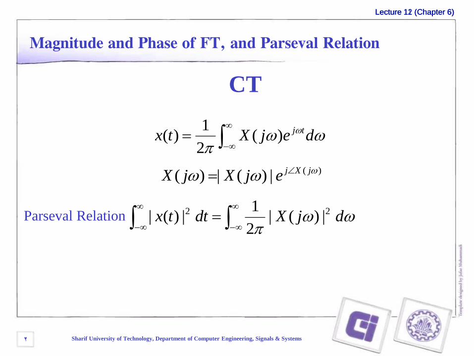
Magnitude and Phase of FT, and Parseval Relation

CT

Parseval Relation

dejXtx tj)(2

1)(

( )( ) | ( ) | j X jX j X j e

djXdttx 22 |)(|

2

1|)(|

Lecture 11 (Chapter 6)Lecture 12 (Chapter 6)

Sharif University of Technology, Department of Computer Engineering, Signals & Systems3

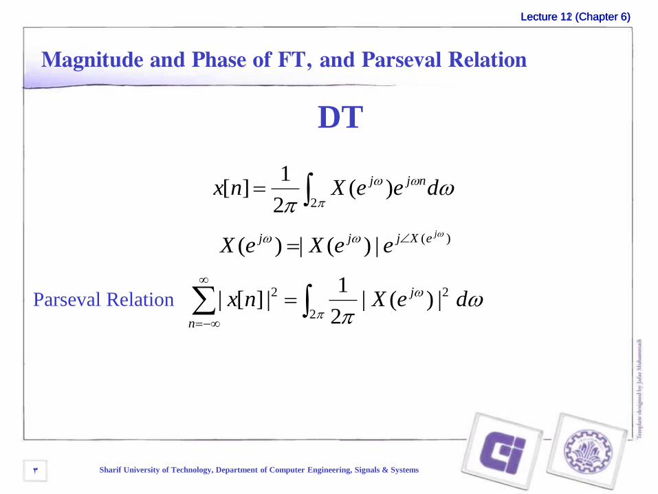
Magnitude and Phase of FT, and Parseval Relation

DT

Parseval Relation

2

)(2

1][ deeXnx njj

)(|)(|)( jeXjjj eeXeX

2

22 |)(|2

1|][| deXnx j

n

Lecture 11 (Chapter 6)Lecture 12 (Chapter 6)

Sharif University of Technology, Department of Computer Engineering, Signals & Systems4

Effects of Phase

• Not on signal energy distribution as a function of frequency

• Can have dramatic effect on signal shape/character

• Constructive/Destructive interference

• Is that important?

• Depends on the signal and the context

Lecture 11 (Chapter 6)Lecture 12 (Chapter 6)

Sharif University of Technology, Department of Computer Engineering, Signals & Systems6

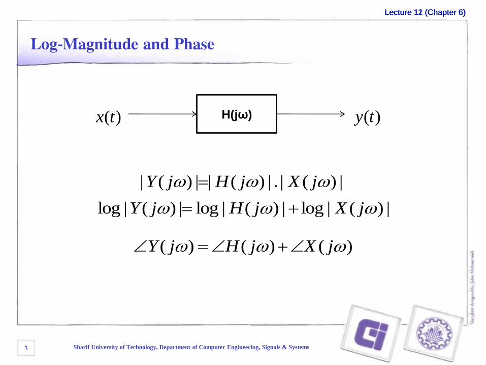
Log-Magnitude and Phase

)(tx H(jω) )(ty

|)(|.|)(||)(| jXjHjY

|)(|log|)(|log|)(|log jXjHjY

)()()( jXjHjY

Lecture 11 (Chapter 6)Lecture 12 (Chapter 6)

Sharif University of Technology, Department of Computer Engineering, Signals & Systems7

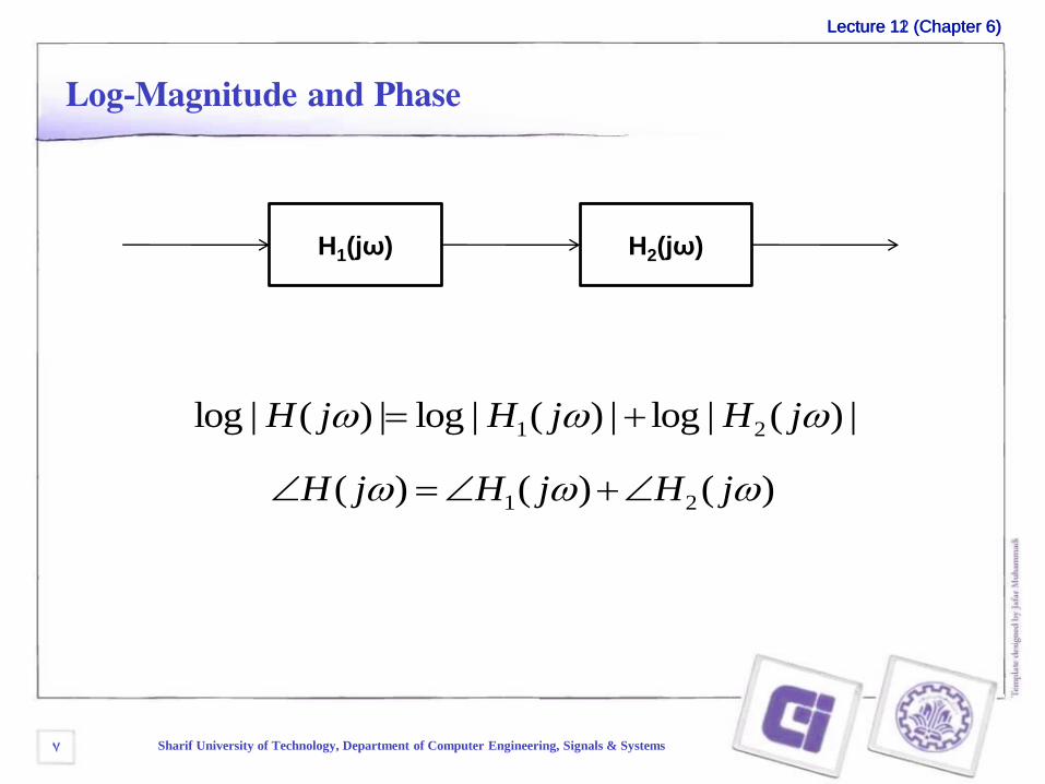
Log-Magnitude and Phase

H1(jω)

|)(|log|)(|log|)(|log 21 jHjHjH

)()()( 21 jHjHjH

H2(jω)

Lecture 11 (Chapter 6)Lecture 12 (Chapter 6)

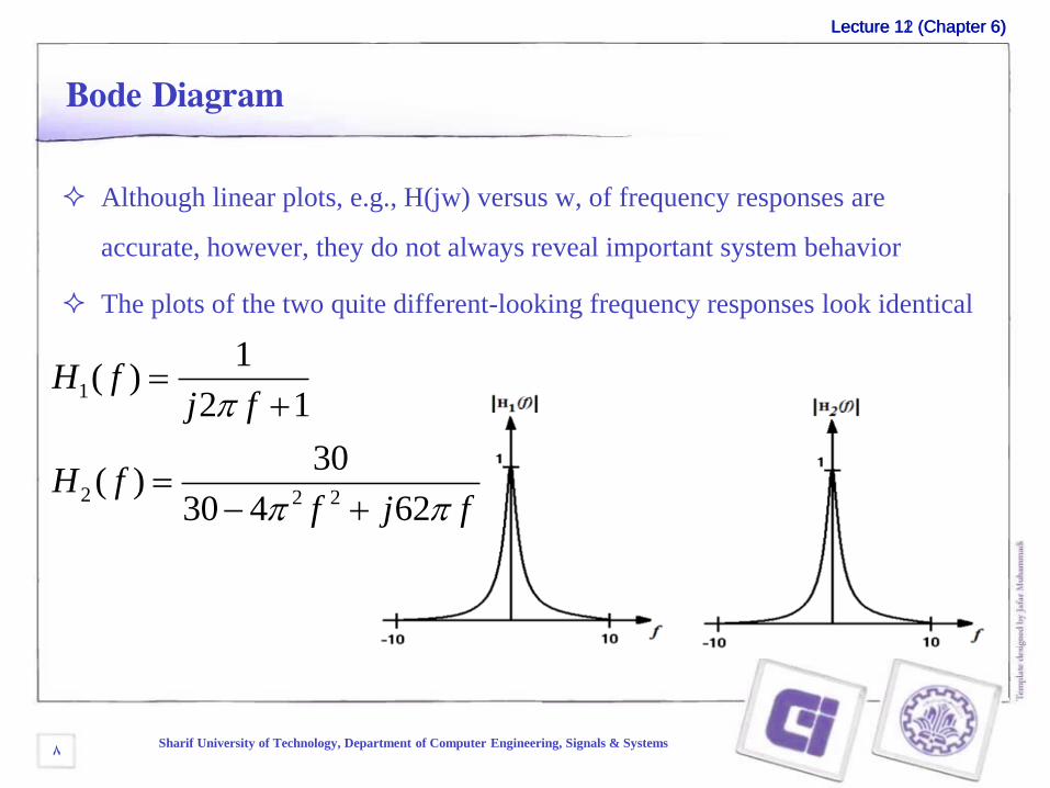
Bode Diagram

Although linear plots, e.g., H(jw) versus w, of frequency responses are

accurate, however, they do not always reveal important system behavior

The plots of the two quite different-looking frequency responses look identical

Sharif University of Technology, Department of Computer Engineering, Signals & Systems8

1

2 2 2

1( )

2 1

30( )

30 4 62

H fj f

H ff j f

Lecture 11 (Chapter 6)Lecture 12 (Chapter 6)

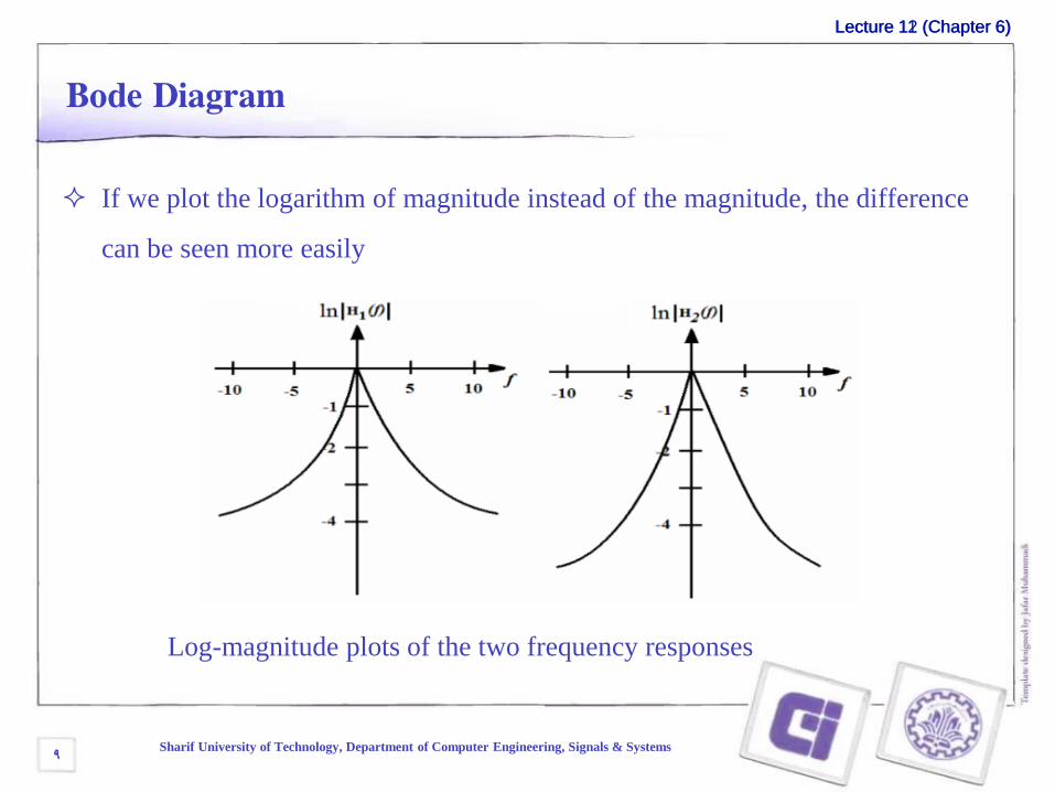
Bode Diagram

If we plot the logarithm of magnitude instead of the magnitude, the difference

can be seen more easily

Log-magnitude plots of the two frequency responses

Sharif University of Technology, Department of Computer Engineering, Signals & Systems9

Lecture 11 (Chapter 6)Lecture 12 (Chapter 6)

Bode diagram

A more common way of displaying frequency response is the Bode diagram or

Bode plot

A log-magnitude plot is logarithmic in one dimension

A Bode diagram is logarithmic in both dimensions

A bode diagram is a plot of the logarithm of the magnitude of a frequency

response against a logarithmic frequency scale

log |H(jw)| versus scaled w

In a bode diagram, |H(jw)| is converted to a logarithmic scale using the unit

decibel (dB)

Sharif University of Technology, Department of Computer Engineering, Signals & Systems10

Lecture 11 (Chapter 6)Lecture 12 (Chapter 6)

Sharif University of Technology, Department of Computer Engineering, Signals & Systems11

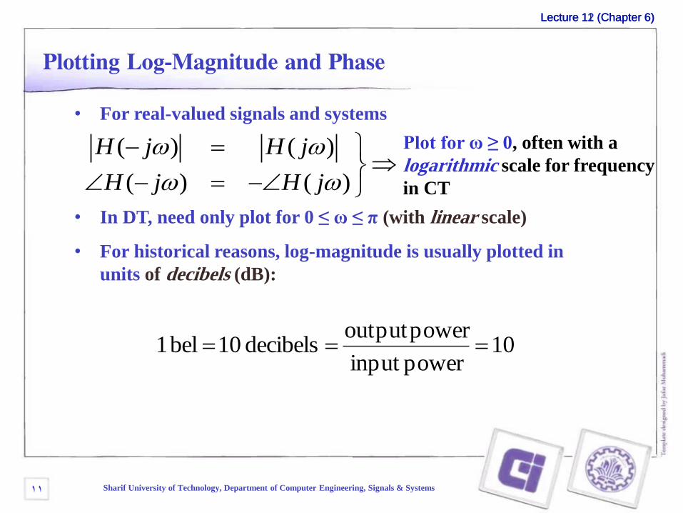
Plotting Log-Magnitude and Phase

• For real-valued signals and systems

Plot for ω ≥ 0, often with a

logarithmic scale for frequency

in CT

• In DT, need only plot for 0 ≤ ω ≤ π (with linear scale)

• For historical reasons, log-magnitude is usually plotted in

units of decibels (dB):

10powerinput

poweroutput decibels 10 bel 1

) )

) ( )

( (

(

H j H j

H j H j

Lecture 11 (Chapter 6)Lecture 12 (Chapter 6)

Sharif University of Technology, Department of Computer Engineering, Signals & Systems12

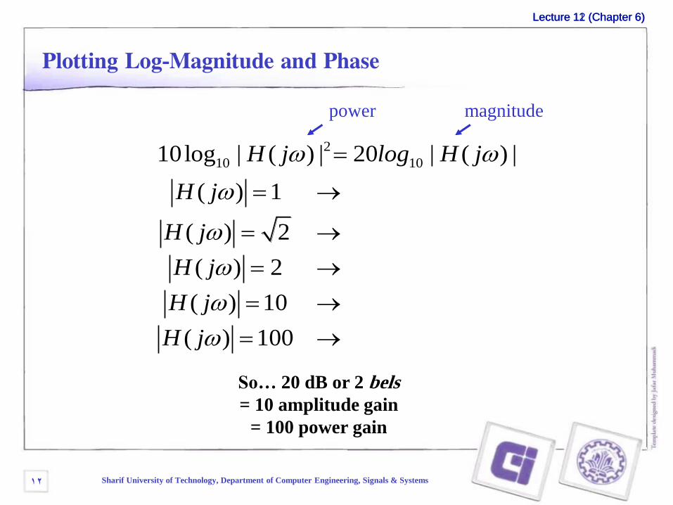
Plotting Log-Magnitude and Phase

power magnitude

So… 20 dB or 2 bels

= 10 amplitude gain

= 100 power gain

2

10 10| ( ) | 20 | (10log

( 1 0

(

( 2

( 10 20

( 100 40

) |

)

) 2 ~ 3

) ~ 6

)

)

H j dB

H j

H j

H j

H j log H j

dB

dB

dB

H j dB

Lecture 11 (Chapter 6)Lecture 12 (Chapter 6)

Sharif University of Technology, Department of Computer Engineering, Signals & Systems13

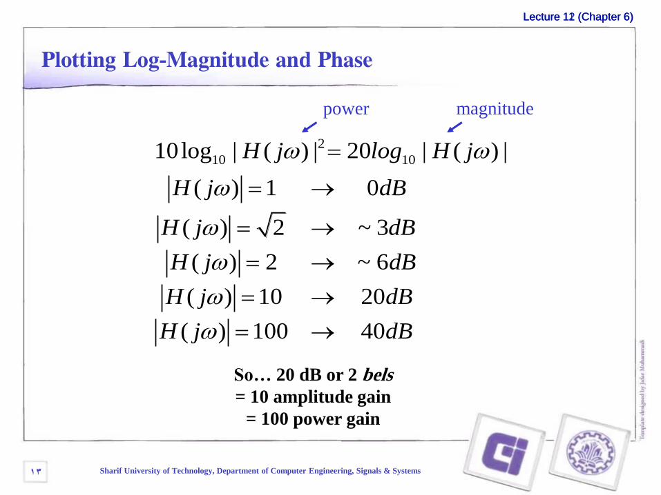
Plotting Log-Magnitude and Phase

power magnitude

So… 20 dB or 2 bels

= 10 amplitude gain

= 100 power gain

2

10 10| ( ) | 20 | (10log

( 1 0

(

( 2

( 10 20

( 100 40

) |

)

) 2 ~ 3

) ~ 6

)

)

H j dB

H j

H j

H j

H j log H j

dB

dB

dB

H j dB

Lecture 11 (Chapter 6)Lecture 12 (Chapter 6)

Sharif University of Technology, Department of Computer Engineering, Signals & Systems14

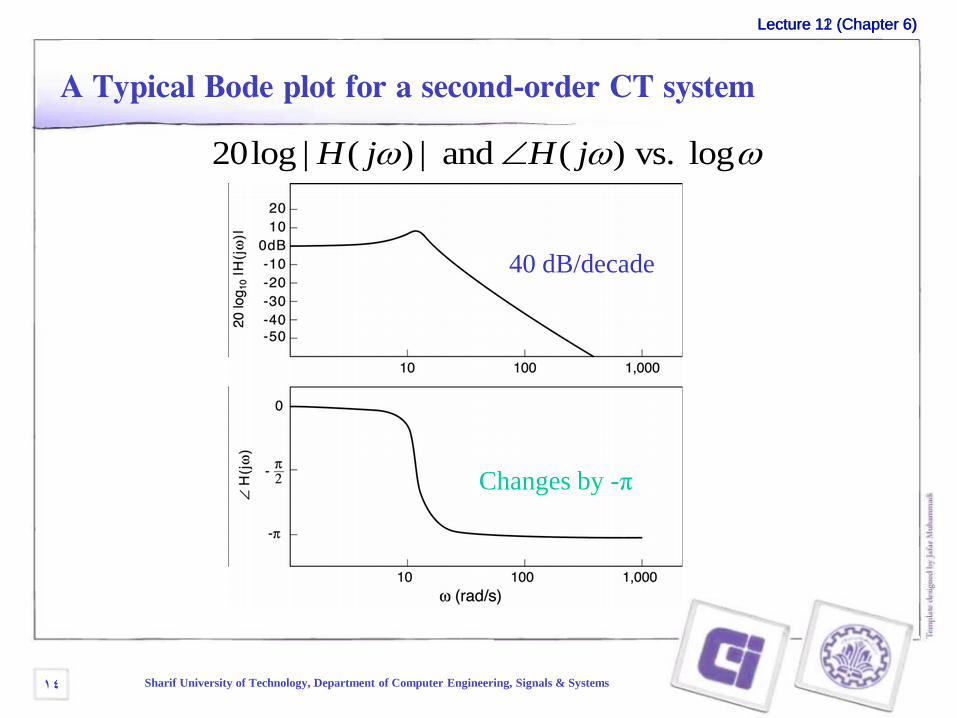
A Typical Bode plot for a second-order CT system

40 dB/decade

Changes by -π

| ( ) | and ( ) vs. log20log H j H j

Lecture 11 (Chapter 6)Lecture 12 (Chapter 6)

Sharif University of Technology, Department of Computer Engineering, Signals & Systems15

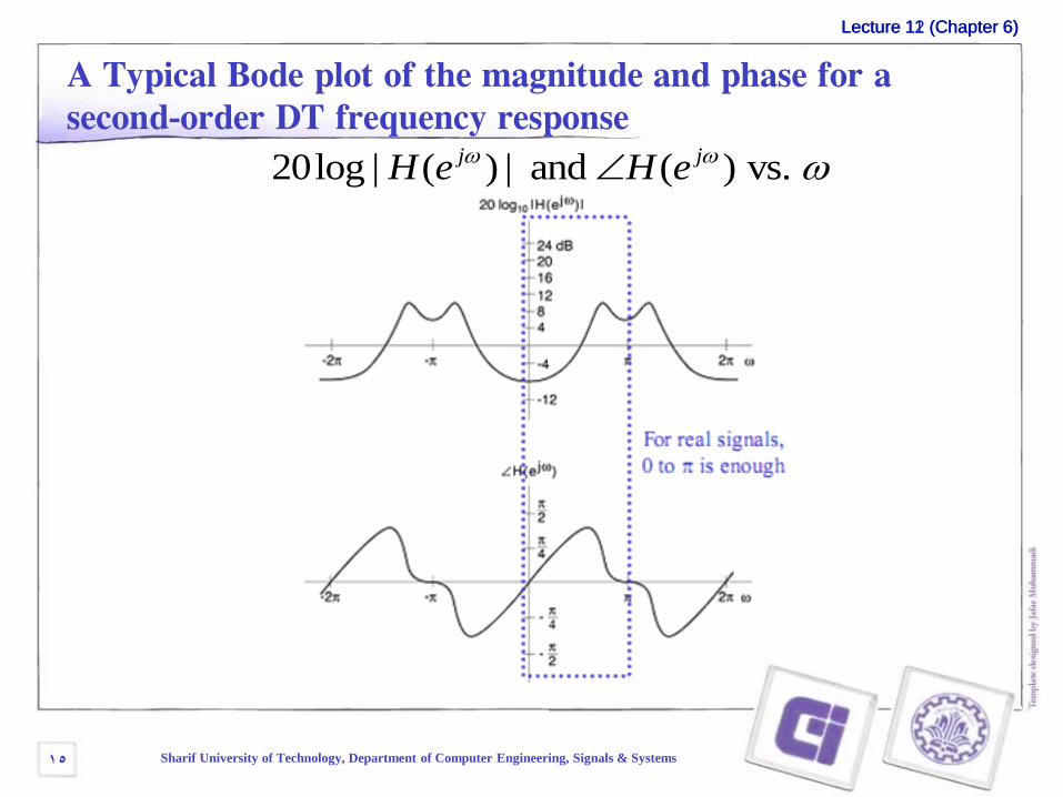
A Typical Bode plot of the magnitude and phase for a

second-order DT frequency response

| ( ) | and ( ) vs. 20log j jH e H e

Lecture 11 (Chapter 6)Lecture 12 (Chapter 6)

Sharif University of Technology, Department of Computer Engineering, Signals & Systems16

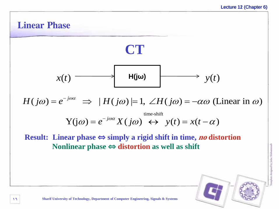
Linear Phase

CT

)(tx H(jω) )(ty

Result: Linear phase ⇔ simply a rigid shift in time, no distortion

Nonlinear phase ⇔ distortion as well as shift

time-shift

) | ( ) | 1, ( ) (Linear ( in )

Y(j ) ( ) (

( ) )

j

j

H j e H j H j

e X j y t x t

Lecture 11 (Chapter 6)Lecture 12 (Chapter 6)

Sharif University of Technology, Department of Computer Engineering, Signals & Systems17

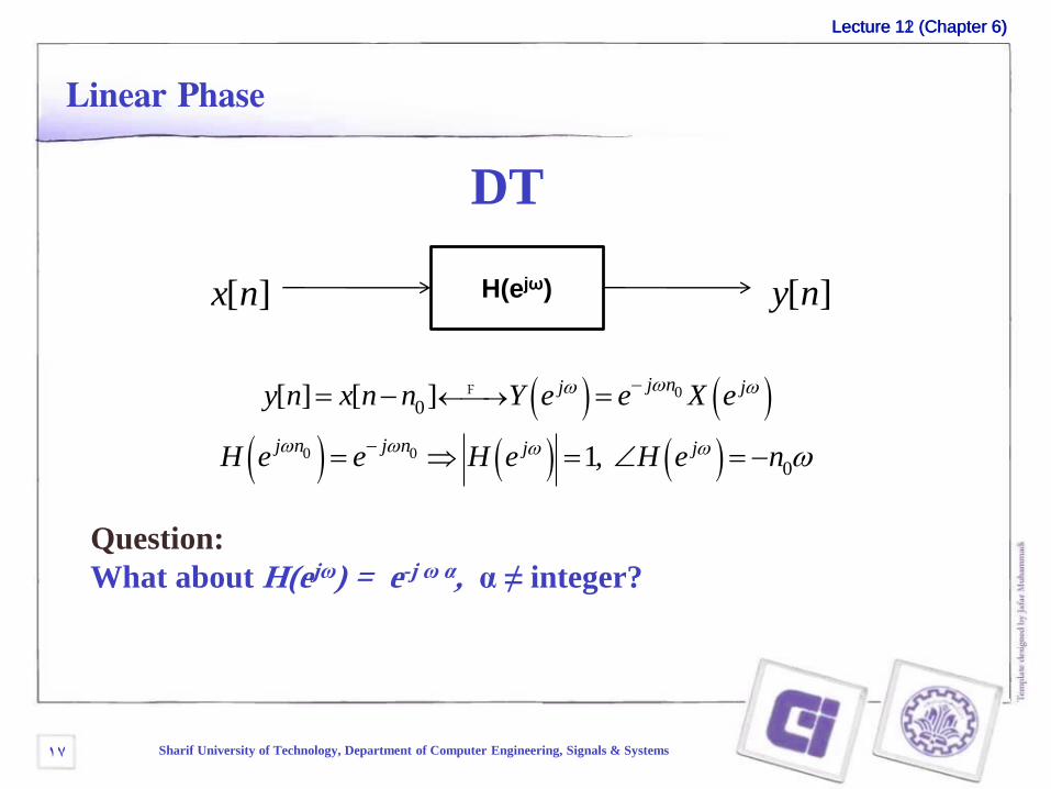
Linear Phase

DT

][nx H(ejω) ][ny

Question:

What about H(ejω) = e-j ω α, α ≠ integer?

0

0 0

0

0

[ ] [ ]

1,

j nj j

j n j n j j

y n x n n Y e e X e

H e e H e H e n

F

Lecture 11 (Chapter 6)Lecture 12 (Chapter 6)

Sharif University of Technology, Department of Computer Engineering, Signals & Systems18

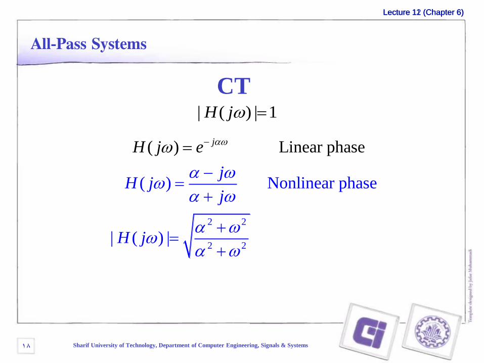
All-Pass Systems

CT1|)(| jH

2 2

2 2

( Linear phas

( ) Nonlinear phase

| ( )

)

|

ej

jH j

j

H

H j e

j

Lecture 11 (Chapter 6)Lecture 12 (Chapter 6)

Sharif University of Technology, Department of Computer Engineering, Signals & Systems19

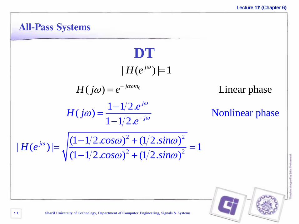
All-Pass Systems

DT1|)(| jeH

0

2 2

2 2

1 1 2.( ) Nonlinear phase

1 1 2.

(1 1 2.

( Linear

) (1 2. )| ( ) | 1

(1 1 2. ) (1 2.

) e

)

phasj

j

j

j

n

eH j

e

cos sinH e

cos sin

j eH

Lecture 11 (Chapter 6)Lecture 12 (Chapter 6)

Sharif University of Technology, Department of Computer Engineering, Signals & Systems21

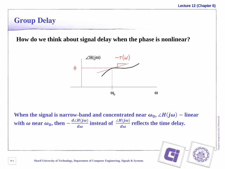
Group Delay

How do we think about signal delay when the phase is nonlinear?

When the signal is narrow-band and concentrated near 𝝎𝟎, ∠𝑯 𝒋𝝎 ∼ linear

with 𝝎 near 𝝎𝟎, then −𝒅∠𝑯(𝒋𝝎)

𝒅𝝎instead of

∠𝑯(𝒋𝝎)

𝒅𝝎reflects the time delay.

Lecture 11 (Chapter 6)Lecture 12 (Chapter 6)

Sharif University of Technology, Department of Computer Engineering, Signals & Systems22

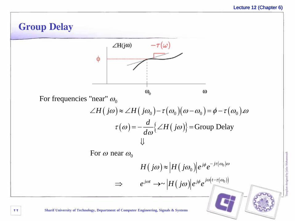
Group Delay

0

0

0

0 0 0 0

0

0

For frequencies "near"

.

Group Delay

For near

~

jj

j tj t j

H j H j

dH j

d

H j H j e e

e H j e e

Lecture 11 (Chapter 6)Lecture 12 (Chapter 6)

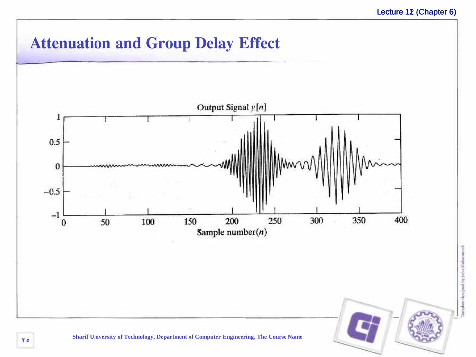
Linear phase / Group delay

Group delay is a measure of the transit time of a signal through a system (or

device) versus frequency

Linear phase is a property of a filter

The phase response of the filter is a linear function of frequency

Linear phase filter has the property of the true time delay

A linear phase filter has constant group delay

All frequency components of a signal have equal delay times

There is no distortion due of select frequencies

A filter with non-linear phase has a group delay that varies with frequency,

resulting in phase distortion

Sharif University of Technology, Department of Computer Engineering, Signals & Systems23

Lecture 11 (Chapter 6)Lecture 12 (Chapter 6)

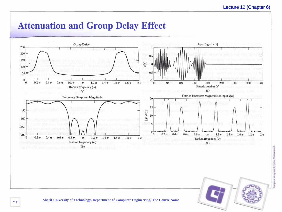
Attenuation and Group Delay Effect

Sharif University of Technology, Department of Computer Engineering, The Course Name24

Lecture 11 (Chapter 6)Lecture 12 (Chapter 6)

Attenuation and Group Delay Effect

Sharif University of Technology, Department of Computer Engineering, The Course Name25