Embed Size (px)
Citation preview


Signals and Communication Technology
For further volumes:http://www.springer.com/series/4748
Hermann RohlingEditor
OFDM
Concepts for Future CommunicationSystems
123

EditorHermann RohlingInstitut für NachrichtentechnikTechnische Universität Hamburg-HarburgEißendorfer Str. 4021073 HamburgGermanye-mail: [email protected]
ISSN 1860-4862
ISBN 978-3-642-17495-7 e-ISBN 978-3-642-17496-4
DOI 10.1007/978-3-642-17496-4
Springer Heidelberg Dordrecht London New York
� Springer-Verlag Berlin Heidelberg 2011
This work is subject to copyright. All rights are reserved, whether the whole or part of thematerial is concerned, specifically the rights of translation, reprinting, reuse of illustrations,recitation, broadcasting, reproduction on microfilm or in any other way, and storage in databanks. Duplication of this publication or parts thereof is permitted only under the provisions ofthe German Copyright Law of September 9, 1965, in its current version, and permission for usemust always be obtained from Springer. Violations are liable to prosecution under the GermanCopyright Law.
The use of general descriptive names, registered names, trademarks, etc. in this publication doesnot imply, even in the absence of a specific statement, that such names are exempt from therelevant protective laws and regulations and therefore free for general use.
Cover design: eStudio Calamar, Belin/Figueres
Printed on acid-free paper
Springer is part of Springer Science+Business Media (www.springer.com)


v
The contents of this book is based on the work of the Priority Pro-gram TakeOFDM (SPP1163), funded by the German Research Foun-dation (Deutsche Forschungsgemeinschaft, DFG).

vii
Preface
Dear readers, dear friends,
The Orthogonal Frequency-Division Multiplexing (OFDM) digital transmissiontechnique has several advantages in broadcast and mobile communications appli-cations. Therefore, the German Research Foundation (DFG) funded a so-calledpriority program “Techniques, Algorithms, and Concepts for Future OFDM Sys-tems” (TakeOFDM), which started in 2004. The main objective of this researchprogram is to study the specific research topics in a collaborative work betweenexperts and young scientists from different universities.
In broadcast applications like Digital Audio Broadcast (DAB), Digital Videobroadcast (DVB-T), Digital Radio Mondiale (DRM), and single-cell WLAN sys-tems,eral years. However, in wireless and wireline communications there is still need forfurther research and optimization. The OFDM transmission technique has gained alot of attention in research, and it has proven to be a suitable choice in the design ofdigital transmission concepts for mobile applications, such as the Long Term Evolu-tion (LTE) standard, which is the system proposal for the fourth generation (4G) ofmobile communication systems. The OFDM transmission method, specific mediumaccess techniques, cellular networks with full coverage, and multiple antenna systemshave been playing an important and ever-growing role in the 4G development.
Since 2004, more than 15 different universities in over 40 specific research projectshave been contributing to the TakeOFDM program, covering a large variety of de-tailed aspects of OFDM and all related system design aspects. This TakeOFDMresearch project led to several PhD theses and is a basis for the young generation ofexcellent scientific researchers and staff. The results have been exchanged in severalworkshops, conferences, and direct cooperations. Besides topics regarding the phys-ical layer, such as coding, modulation, and non-linearities, a special emphasis wasput on system aspects and concepts, in particular focusing on cellular networks andmultiple antenna techniques. The challenges of link adaptation, adaptive resourceallocation, and interference mitigation in such systems were addressed extensively.Moreover, the domain of cross-layer design, i.e., the combination of physical layeraspects and issues of higher layers, was considered in detail.
This book summarizes the main results and gives an overview of the combined re-search efforts which have been undertaken in the past 6 years within the TakeOFDM
gratitude to the German Research Foundation (DFG) for their generous funding,continuous support and fruitful collaboration throughout the lifetime of the Take-OFDM project. Moreover, my sincere thanks go to all scientists for their excellentwork on a high scientific level and their valuable contributions over the last years.
the OFDM transmission technique is already mature and operational for sev-
I would like to express mypriority program. he program,As a coordinator of t
viii Preface
The aim of this book is to give a good insight into these efforts, and provide thereader with a comprehensive overview of the scientific progress which was achievedin the framework of TakeOFDM. I am convinced that also in the future, these resultswill facilitate and stimulate further innovation and developments in the design ofmodern communication systems, based on the powerful OFDM transmission tech-nique.
Prof. Dr. Hermann Rohling Hamburg, June 2010
ix
Contents
1 Introduction . . . . . . . . . . . . . . . . . . . . . . . . . . . . . . . . . . . . . . . . 11.1 Radio Channel Behavior . . . . . . . . . . . . . . . . . . . . . . . . . . . 21.2 Basics of the OFDM Transmission Technique . . . . . . . . . . . 51.3 OFDM Combined with Multiple Access Schemes . . . . . . . . 10
2 Channel Modeling . . . . . . . . . . . . . . . . . . . . . . . . . . . . . . . . . . . . 152.1 Joint Space-Time-Frequency Representation . . . . . . . . . . . . 16
2.1.1 Multidimensional Channel Sounding . . . . . . . . . . . . 172.1.2 Extraction of Parameters for Dominant MPCs . . . . 17
2.2 Deterministic Modeling . . . . . . . . . . . . . . . . . . . . . . . . . . . 182.2.1 Relevant GTD/UTD Aspects . . . . . . . . . . . . . . . . . 182.2.2 Vechicle2X Channel Modeling . . . . . . . . . . . . . . . . 19
2.3 Stochastic Driving of Multi-Path Model . . . . . . . . . . . . . . . 202.3.1 Usage of the Large-Scale Parameters for Channel
Characterization. . . . . . . . . . . . . . . . . . . . . . . . . . . 212.3.2 Relaying . . . . . . . . . . . . . . . . . . . . . . . . . . . . . . . . 242.3.3 Cooperative Downlink . . . . . . . . . . . . . . . . . . . . . . 24
3 Link-Level Aspects. . . . . . . . . . . . . . . . . . . . . . . . . . . . . . . . . . . . 333.1 OFDM Data Detection and Channel Estimation . . . . . . . . . 33
3.1.1 Introduction . . . . . . . . . . . . . . . . . . . . . . . . . . . . . . 333.1.2 Data Detection in the Presence
of Nonlinear Distortions . . . . . . . . . . . . . . . . . . . . . 333.1.3 Joint Data Detection and Channel Estimation . . . . 39
3.2 Spreading . . . . . . . . . . . . . . . . . . . . . . . . . . . . . . . . . . . . . . 473.2.1 Introduction . . . . . . . . . . . . . . . . . . . . . . . . . . . . . . 473.2.2 MC-CDM and MC-CAFS . . . . . . . . . . . . . . . . . . . . 483.2.3 Simulation Results . . . . . . . . . . . . . . . . . . . . . . . . . 493.2.4 Concluding Remarks . . . . . . . . . . . . . . . . . . . . . . . 51

x Contents
3.3 Iterative Diversity Reception for Coded OFDMTransmission Over Fading Channels . . . . . . . . . . . . . . . . . . 543.3.1 Introduction . . . . . . . . . . . . . . . . . . . . . . . . . . . . . . 543.3.2 Turbo Diversity . . . . . . . . . . . . . . . . . . . . . . . . . . . 553.3.3 Optimization for Turbo Diversity . . . . . . . . . . . . . . 563.3.4 Performance Evaluation . . . . . . . . . . . . . . . . . . . . . 573.3.5 Summary . . . . . . . . . . . . . . . . . . . . . . . . . . . . . . . . 59
3.4 MMSE-based Turbo Equalization Principles for FrequencySelective Fading Channels . . . . . . . . . . . . . . . . . . . . . . . . . 613.4.1 Introduction . . . . . . . . . . . . . . . . . . . . . . . . . . . . . . 613.4.2 System Model . . . . . . . . . . . . . . . . . . . . . . . . . . . . 613.4.3 MMSE Turbo Equalization Principles. . . . . . . . . . . 623.4.4 Summary . . . . . . . . . . . . . . . . . . . . . . . . . . . . . . . . 66
3.5 Peak-to-Average Power Ratio Reduction in Multi-AntennaScenarios . . . . . . . . . . . . . . . . . . . . . . . . . . . . . . . . . . . . . . 693.5.1 Introduction and Overview on PAR
Reduction Schemes . . . . . . . . . . . . . . . . . . . . . . . . 693.5.2 PAR Reduction Schemes for MIMO
Transmission . . . . . . . . . . . . . . . . . . . . . . . . . . . . . 713.5.3 Numerical Results . . . . . . . . . . . . . . . . . . . . . . . . . 743.5.4 Summary . . . . . . . . . . . . . . . . . . . . . . . . . . . . . . . . 74
3.6 Single- vs. Multicarrier Transmission in MIMOand Multiuser Scenarios . . . . . . . . . . . . . . . . . . . . . . . . . . . 813.6.1 Introduction . . . . . . . . . . . . . . . . . . . . . . . . . . . . . . 813.6.2 Point-to-Point MIMO Transmission . . . . . . . . . . . . 813.6.3 Up- and Downlink Scenarios in Multiuser
Transmission . . . . . . . . . . . . . . . . . . . . . . . . . . . . . 823.6.4 Aspects of Channel Coding . . . . . . . . . . . . . . . . . . . 843.6.5 Summary . . . . . . . . . . . . . . . . . . . . . . . . . . . . . . . . 85
3.7 Successive Bit Loading Concept . . . . . . . . . . . . . . . . . . . . . 903.7.1 Introduction . . . . . . . . . . . . . . . . . . . . . . . . . . . . . . 903.7.2 System Model . . . . . . . . . . . . . . . . . . . . . . . . . . . . 913.7.3 Bit Loading Algorithm . . . . . . . . . . . . . . . . . . . . . . 923.7.4 Results. . . . . . . . . . . . . . . . . . . . . . . . . . . . . . . . . . 943.7.5 Summary . . . . . . . . . . . . . . . . . . . . . . . . . . . . . . . . 96
3.8 Adaptive Transmission Techniques . . . . . . . . . . . . . . . . . . . 983.8.1 Introduction . . . . . . . . . . . . . . . . . . . . . . . . . . . . . . 983.8.2 Adaptive Modulation and Coding . . . . . . . . . . . . . . 983.8.3 Adaptive MIMO Transmission . . . . . . . . . . . . . . . . 993.8.4 Signaling of the Bit Allocation Table . . . . . . . . . . . 1023.8.5 Automatic Modulation Classification . . . . . . . . . . . 1033.8.6 Summary . . . . . . . . . . . . . . . . . . . . . . . . . . . . . . . . 105
Contents xi
4 System Level Aspects for Single Cell Scenarios . . . . . . . . . . . . . . 1094.1 Efficient Analysis of OFDM Channels . . . . . . . . . . . . . . . . . 109
4.1.1 Introduction . . . . . . . . . . . . . . . . . . . . . . . . . . . . . . 1094.1.2 The Channel Matrix G . . . . . . . . . . . . . . . . . . . . . . 1094.1.3 Common Channel Operator Models . . . . . . . . . . . . 1114.1.4 Computing the Channel Matrix G . . . . . . . . . . . . . 112
4.2 Generic Description of a MIMO-OFDM-Radio-Transmission-Link . . . . . . . . . . . . . . . . . . . . . . . . . . . . . . . 1154.2.1 Introduction . . . . . . . . . . . . . . . . . . . . . . . . . . . . . . 1154.2.2 System Model . . . . . . . . . . . . . . . . . . . . . . . . . . . . 1154.2.3 Performance Analysis . . . . . . . . . . . . . . . . . . . . . . . 1164.2.4 Generic Model . . . . . . . . . . . . . . . . . . . . . . . . . . . . 1184.2.5 Summary and Further Work . . . . . . . . . . . . . . . . . 120
4.3 Resource Allocation Using Broadcast Techniques . . . . . . . . 1224.3.1 Motivation . . . . . . . . . . . . . . . . . . . . . . . . . . . . . . . 1224.3.2 Resource Allocation Algorithms . . . . . . . . . . . . . . . 122
4.4 Rate Allocation for the 2-User Multiple Access Channelwith MMSE Turbo Equalization . . . . . . . . . . . . . . . . . . . . . 1284.4.1 Introduction . . . . . . . . . . . . . . . . . . . . . . . . . . . . . . 1284.4.2 Turbo Equalization . . . . . . . . . . . . . . . . . . . . . . . . 1284.4.3 Rate Allocation using EXIT Charts . . . . . . . . . . . . 1294.4.4 Summary . . . . . . . . . . . . . . . . . . . . . . . . . . . . . . . . 131
4.5 Coexistence of Systems . . . . . . . . . . . . . . . . . . . . . . . . . . . . 1334.6 System Design for Time-Variant Channels . . . . . . . . . . . . . 136
4.6.1 Multicarrier Systems for Rapidly MovingReceivers . . . . . . . . . . . . . . . . . . . . . . . . . . . . . . . . 136
4.6.2 Highly Mobile MIMO-OFDM-Transmission inRealistic Propagation Scenarios . . . . . . . . . . . . . . . 138
4.7 Combination of Adaptive and Non-Adaptive Multi-UserOFDMA Schemes in the Presence of User-DependentImperfect CSI. . . . . . . . . . . . . . . . . . . . . . . . . . . . . . . . . . . 1424.7.1 Introduction . . . . . . . . . . . . . . . . . . . . . . . . . . . . . . 1424.7.2 Combining Transmission Schemes . . . . . . . . . . . . . 1424.7.3 Numerical Results . . . . . . . . . . . . . . . . . . . . . . . . . 143
4.8 Integration of COFDM Systems with Multiple Antennasand Design of Adaptive Medium Access Protocols . . . . . . . 1464.8.1 Abstract . . . . . . . . . . . . . . . . . . . . . . . . . . . . . . . . 1464.8.2 MAC Frame for SDMA Operation and Spatial
Grouping . . . . . . . . . . . . . . . . . . . . . . . . . . . . . . . . 1464.8.3 Hardware Implementation of COFDM Systems
with Multiple Antennas . . . . . . . . . . . . . . . . . . . . . 1474.9 Large System Analysis of Nearly Optimum Low Complex
Beamforming in Multicarrier MultiuserMultiantenna Systems . . . . . . . . . . . . . . . . . . . . . . . . . . . . 150

xii Contents
4.9.1 Introduction . . . . . . . . . . . . . . . . . . . . . . . . . . . . . . 1504.9.2 System Model . . . . . . . . . . . . . . . . . . . . . . . . . . . . 1504.9.3 Description of Algorithms. . . . . . . . . . . . . . . . . . . . 1514.9.4 Approximation of the Ergodic Sum Rate with
Large System Analysis . . . . . . . . . . . . . . . . . . . . . . 1524.9.5 Numerical Results . . . . . . . . . . . . . . . . . . . . . . . . . 154
4.10 Combined Radar and Communication SystemsUsing OFDM . . . . . . . . . . . . . . . . . . . . . . . . . . . . . . . . . . . 1564.10.1 Introduction . . . . . . . . . . . . . . . . . . . . . . . . . . . . . . 1564.10.2 Signal Design . . . . . . . . . . . . . . . . . . . . . . . . . . . . . 1564.10.3 The Radar Subsystem . . . . . . . . . . . . . . . . . . . . . . 1584.10.4 Measurements . . . . . . . . . . . . . . . . . . . . . . . . . . . . 1604.10.5 Summary . . . . . . . . . . . . . . . . . . . . . . . . . . . . . . . . 163
5 System Level Aspects for Multiple Cell Scenarios. . . . . . . . . . . . . 1655.1 Link Adaptation. . . . . . . . . . . . . . . . . . . . . . . . . . . . . . . . . 165
5.1.1 Motivation . . . . . . . . . . . . . . . . . . . . . . . . . . . . . . . 1655.1.2 Example of a Multiple Link Scenario . . . . . . . . . . . 1655.1.3 Adaptation of Physical Link Parameters. . . . . . . . . 1695.1.4 Cross-Layer Adaptation . . . . . . . . . . . . . . . . . . . . . 1765.1.5 Multiple Link Network - Overall Adaptation . . . . . 178
5.2 System Concept for aData Transmission Network . . . . . . . . . . . . . . . . . . . . . . . . 1805.2.1 Introduction . . . . . . . . . . . . . . . . . . . . . . . . . . . . . . 1805.2.2 Beamforming Concepts. . . . . . . . . . . . . . . . . . . . . . 1815.2.3 System Concept . . . . . . . . . . . . . . . . . . . . . . . . . . . 1825.2.4 Summary . . . . . . . . . . . . . . . . . . . . . . . . . . . . . . . . 190
5.3 Pricing Algorithms for Power Control, Beamformer Design,and Interference Alignment in InterferenceLimited Networks. . . . . . . . . . . . . . . . . . . . . . . . . . . . . . . . 1925.3.1 Introduction . . . . . . . . . . . . . . . . . . . . . . . . . . . . . . 1925.3.2 System Model . . . . . . . . . . . . . . . . . . . . . . . . . . . . 1925.3.3 Distributed Interference Pricing . . . . . . . . . . . . . . . 1935.3.4 MIMO Interference Networks and
Interference Alignment . . . . . . . . . . . . . . . . . . . . . . 1965.3.5 Summary . . . . . . . . . . . . . . . . . . . . . . . . . . . . . . . . 198
5.4 Interference Reduction: Cooperative Communicationwith Partial CST in Mobile Radio Cellular Networks . . . . . 1995.4.1 Introduction . . . . . . . . . . . . . . . . . . . . . . . . . . . . . . 1995.4.2 System Model and Reference Scenario . . . . . . . . . . 2005.4.3 Significant CSI Selection Algorithm and Channel
Matrix Formalism . . . . . . . . . . . . . . . . . . . . . . . . . 2035.4.4 Decentralized JD/JT with Significant CSI for
Interference Reduction . . . . . . . . . . . . . . . . . . . . . . 205
MIMO-OFDM-Based Self-Organizing
Contents xiii
5.4.5 Impact of Imperfect CSI on CooperativeCommunication Based on JD/JT . . . . . . . . . . . . . . 208
5.4.6 Advanced Algorithm Based on StatisticalKnowledge of Imperfect CSI . . . . . . . . . . . . . . . . . . 210
5.4.7 System Concept Based on Different Levels ofKnowledge of CSI . . . . . . . . . . . . . . . . . . . . . . . . . 211
5.4.8 Outlook . . . . . . . . . . . . . . . . . . . . . . . . . . . . . . . . . 211
6 OFDM/DMT for Wireline Communications . . . . . . . . . . . . . . . . . 2156.1 Discrete MultiTone (DMT) and Wireline
Channel Properties . . . . . . . . . . . . . . . . . . . . . . . . . . . . . . . 2156.1.1 Properties of the Twisted-Pair Channel . . . . . . . . . 2156.1.2 Discrete MultiTone (DMT) . . . . . . . . . . . . . . . . . . 219
6.2 Optical OFDM Transmission and OpticalChannel Properties . . . . . . . . . . . . . . . . . . . . . . . . . . . . . . . 225
6.3 Impulse-Noise Cancellation . . . . . . . . . . . . . . . . . . . . . . . . . 2276.3.1 Common Mode and Differential Mode . . . . . . . . . . 2276.3.2 Coupling and Transfer Functions . . . . . . . . . . . . . . 2276.3.3 Common-Mode Reference-Based Canceler. . . . . . . . 2276.3.4 Impulse Noise Detection and Cancellation . . . . . . . 2296.3.5 Simulation Results . . . . . . . . . . . . . . . . . . . . . . . . . 230
6.4 Dual Polarization Optical OFDM Transmission . . . . . . . . . 2336.4.1 Setup . . . . . . . . . . . . . . . . . . . . . . . . . . . . . . . . . . . 2336.4.2 Noise Variance Estimation . . . . . . . . . . . . . . . . . . . 2346.4.3 ADC/DAC Resolution . . . . . . . . . . . . . . . . . . . . . . 237
6.5 Forward Error Correction. . . . . . . . . . . . . . . . . . . . . . . . . . 2386.5.1 BICM-ID System Model . . . . . . . . . . . . . . . . . . . . . 2396.5.2 Influence of the Applied Mapping . . . . . . . . . . . . . . 2416.5.3 Simulations on the Performance
of Coded OFDM . . . . . . . . . . . . . . . . . . . . . . . . . . 2416.6 Summary . . . . . . . . . . . . . . . . . . . . . . . . . . . . . . . . . . . . . . 243
Index . . . . . . . . . . . . . . . . . . . . . . . . . . . . . . . . . . . . . . . . . . . . . . . . 251


H. Rohling (ed.), OFDM: Concepts for Future Communication Systems, 1Signals and Communication Technology, DOI: 10.1007/978-3-642-17496-4_1,© Springer-Verlag Berlin Heidelberg 2011
1 Introduction
H. Rohling, Hamburg University of Technology, Germany
In the evolution of mobile communication systems, approximately a 10 years pe-riodicity can be observed between consecutive system generations. Research workfor the current 2nd generation of mobile communication systems (GSM) started inEurope in the early 1980s, and the complete system was ready for market in 1990.At that time, the first research activities had already been started for the 3rd gener-ation (3G) of mobile communication systems (UMTS, IMT-2000) and the transitionfrom second generation (GSM) to the new 3G systems was observed around 2002.Compared to today’s GSM networks, these UMTS systems provide much higher datarates, typically in the range of 64 to 384 kbit/s, while the peak data rate for low mo-bility or indoor applications is 2 Mbit/s. With the extension of High Speed PacketAccess (HSPA), data rates of up to 7.2 Mbit/s are available in the downlink. Thecurrent pace, which can be observed in the mobile communications market, alreadyshows that the 3G systems will not be the ultimate system solution. Consequently,general requirements for a fourth generation (4G) system have been considered inthe process of the “Long Term Evolution” (LTE) standardization. These require-ments have mainly been derived from the types of service a user will require infuture applications. Generally, it is expected that data services instead of pure voiceservices will play a predominant role, in particular due to a demand for mobile IPapplications. Variable and especially high data rates (100 Mbps and more) will berequested, which should also be available at high mobility in general or high vehiclespeeds in particular (see Fig. 1.1). Moreover, asymmetrical data services betweenup- and downlink are assumed and should be supported by LTE systems in such ascenario where the downlink carries most of the traffic and needs the higher datarate compared to the uplink.
To fulfill all these detailed system requirements, the OFDM transmission tech-nique applied in a wide-band radio channel has been chosen as an air interface forthe downlink in the framework of LTE standardization due to its flexibility andadaptivity in the technical system design. From the above considerations, it alreadybecomes apparent that a radio transmission system for LTE must provide a greatflexibility and adaptivity at different levels, ranging from the highest layer (require-ments of the application) to the lowest layer (the transmission medium, the physicallayer ,i.e., the radio channel) in the ISO-OSI stack. Today, the OFDM transmissiontechnique is in a completely matured stage to be applied for wide-band communi-cation systems integrated into a cellular mobile communications environment.

2 1 Introduction
Figure 1.1: General requirements for 4G mobile communication systems
Transmitter
Receiver
Figure 1.2: Multipath propagation scenario
1.1 Radio Channel Behavior
The mobile communication system design is in general always dominated by theradio channel behavior [19] [25]. In a typical radio channel situation, multi-pathpropagation occurs (Fig. 1.2) due to the reflections of the transmitted signal atseveral objects and obstacles inside the local environment and inside the observationarea. The radio channel is analytically described unambiguously by a linear (quasi)time-invariant (LTI) system model and by the related channel impulse responseh(τ) or, alternatively, by the channel transfer function H(f ). An example for thesechannel characteristics is shown in Fig. 1.3, where h(τ) and H(f ) of a so-calledWide-Sense Stationary, Uncorrelated Scattering-channel (WSSUS) are given.
Due to the mobility of the mobile terminals, the multipath propagation situationwill be continuously but slowly changed over time which is described analyticallyby a time-variant channel impulse response h(τ, t) or alternatively by a frequency-
1.1 Radio Channel Behavior 3
0 1 2 3 4 5 6 7 8 9 10-30
-20
-10
0
10
|H(f
)|/dB
f / MHz
sTS �� 55max ���
� ��h�
dB0
dB30ST ST2 ST3 ST4 ST50 �
0 1 2 3 4 5 6 7 8 9 10-30
-20
-10
0
10
|H(f
)|/dB
f / MHz
sTS �� 55max ���
0 1 2 3 4 5 6 7 8 9 10-30
-20
-10
0
10
|H(f
)|/dB
f / MHz
sTS �� 55max ���
� ��h�
dB0
dB30ST ST2 ST3 ST4 ST50 �
� ��h�
dB0
dB30ST ST2 ST3 ST4 ST50 �
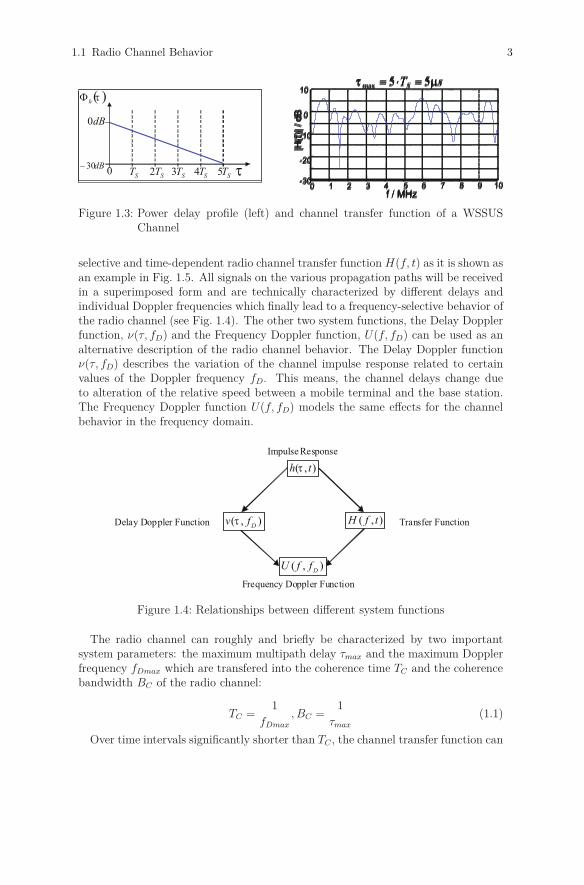
Figure 1.3: Power delay profile (left) and channel transfer function of a WSSUSChannel
selective and time-dependent radio channel transfer function H(f, t) as it is shown asan example in Fig. 1.5. All signals on the various propagation paths will be receivedin a superimposed form and are technically characterized by different delays andindividual Doppler frequencies which finally lead to a frequency-selective behavior ofthe radio channel (see Fig. 1.4). The other two system functions, the Delay Dopplerfunction, ν(τ, fD) and the Frequency Doppler function, U(f, fD) can be used as analternative description of the radio channel behavior. The Delay Doppler functionν(τ, fD) describes the variation of the channel impulse response related to certainvalues of the Doppler frequency fD. This means, the channel delays change dueto alteration of the relative speed between a mobile terminal and the base station.The Frequency Doppler function U(f, fD) models the same effects for the channelbehavior in the frequency domain.
( , )h t�
( , )D
U f f
( , )H f t( , )D
v f� Transfer FunctionDelay Doppler Function
Impulse Response
Frequency Doppler Function
Figure 1.4: Relationships between different system functions
The radio channel can roughly and briefly be characterized by two importantsystem parameters: the maximum multipath delay τmax and the maximum Dopplerfrequency fDmax which are transfered into the coherence time TC and the coherencebandwidth BC of the radio channel:
TC =1
fDmax
, BC =1
τmax
(1.1)
Over time intervals significantly shorter than TC , the channel transfer function can

4 1 Introduction
be assumed to be almost stationary. Similarly, for frequency intervals significantlysmaller than BC , the channel transfer function can be considered as nearly constant.Therefore, it is assumed in this chapter that the coherence time TC is much largercompared to a single OFDM symbol duration TS and the coherence bandwidth BC
is much larger than the distance Δf between two adjacent subcarriers:
BC � Δf, Δf =1
TS, TS � TC (1.2)
This condition should always be fulfilled in well-dimensioned OFDM systems andin realistic time-variant and frequency-selective radio channels.
Figure 1.5: Frequency-selective and time-variant radio channel transfer function
There are always technical alternatives possible in new system design phases.However, future mobile communication systems will in any case require extremelylarge data rates and therefore large system bandwidth. If conventional single carrier(SC) modulation schemes with the resulting very low symbol durations are appliedin this system design, very strong intersymbol interference (ISI) is caused in wide-band applications due to multi-path propagation situations. This means, for highdata rate applications, the symbol duration in a classical SC transmission systemis extremely small compared to the typical values of maximum multi-path delayτmax in the considered radio channel. In these strong ISI situations, a very powerfulequalizer is necessary in each receiver, which needs high computation complexity ina wide-band system. These constraints should be taken into consideration in thesystem development phase for a new radio transmission scheme. The computationalcomplexity for the necessary equalizer techniques to overcome all these strong ISIin a SC modulation scheme increases quadratically for a given radio channel withincreasing system bandwidth and can be extremely large in wide-band applications.For that reason alternative transmission techniques for broadband applications areof high interest.
1.1 Radio Channel Behavior 5
Alternatively, OFDM can efficiently deal with all these ISI effects, which occur inmulti-path propagation situations and in broadband radio channels. Simultaneously,the OFDM transmission technique needs much less computational complexity in theequalization process inside each receiver. The performance figures for an OFDMbased new air interface and for next generation of mobile communications are verypromising even in frequency-selective and time-variant radio channels.
1.2 Basics of the OFDM Transmission Technique
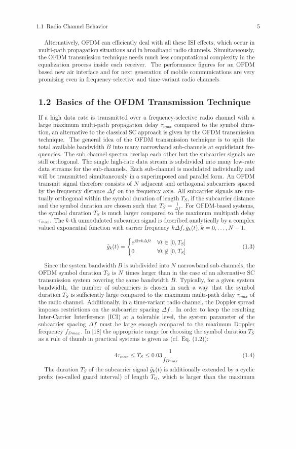
If a high data rate is transmitted over a frequency-selective radio channel with alarge maximum multi-path propagation delay τmax compared to the symbol dura-tion, an alternative to the classical SC approach is given by the OFDM transmissiontechnique. The general idea of the OFDM transmission technique is to split thetotal available bandwidth B into many narrowband sub-channels at equidistant fre-quencies. The sub-channel spectra overlap each other but the subcarrier signals arestill orthogonal. The single high-rate data stream is subdivided into many low-ratedata streams for the sub-channels. Each sub-channel is modulated individually andwill be transmitted simultaneously in a superimposed and parallel form. An OFDMtransmit signal therefore consists of N adjacent and orthogonal subcarriers spacedby the frequency distance Δf on the frequency axis. All subcarrier signals are mu-tually orthogonal within the symbol duration of length TS, if the subcarrier distanceand the symbol duration are chosen such that TS = 1
Δf . For OFDM-based systems,the symbol duration TS is much larger compared to the maximum multipath delayτmax. The k-th unmodulated subcarrier signal is described analytically by a complexvalued exponential function with carrier frequency kΔf, gk(t), k = 0, . . . , N − 1.
gk(t) =
⎧⎨⎩ej2πkΔft ∀t ∈ [0, TS]
0 ∀t �∈ [0, TS](1.3)
Since the system bandwidth B is subdivided into N narrowband sub-channels, theOFDM symbol duration TS is N times larger than in the case of an alternative SCtransmission system covering the same bandwidth B. Typically, for a given systembandwidth, the number of subcarriers is chosen in such a way that the symbolduration TS is sufficiently large compared to the maximum multi-path delay τmax ofthe radio channel. Additionally, in a time-variant radio channel, the Doppler spreadimposes restrictions on the subcarrier spacing Δf . In order to keep the resultingInter-Carrier Interference (ICI) at a tolerable level, the system parameter of thesubcarrier spacing Δf must be large enough compared to the maximum Dopplerfrequency fDmax. In [18] the appropriate range for choosing the symbol duration TS
as a rule of thumb in practical systems is given as (cf. Eq. (1.2)):
4τmax ≤ TS ≤ 0.031
fDmax
(1.4)
The duration TS of the subcarrier signal gk(t) is additionally extended by a cyclicprefix (so-called guard interval) of length TG, which is larger than the maximum

6 1 Introduction
multi-path delay τmax in order to avoid ISI completely which could occur in multi-path channels in the transition interval between two adjacent OFDM symbols [17].
gk(t) =
⎧⎨⎩ej2πkΔft ∀t ∈ [−TG, TS ]
0 ∀t �∈ [−TG, TS ](1.5)
The guard interval is directly removed in the receiver after the time synchro-nization procedure. From this point of view, the guard interval is a pure systemoverhead. The total OFDM symbol duration is therefore T = TS + TG. It is animportant advantage of the OFDM transmission technique that ISI can be avoidedcompletely or can be reduced at least considerably by a proper choice of OFDMsystem parameters.
The orthogonality of all subcarrier signals is completely preserved in the receivereven in frequency-selective radio channels, which is an important advantage ofOFDM. The radio channel behaves linearly and in a short time interval of a fewOFDM symbols even time-invariant. Hence, the radio channel behavior can bedescribed completely by a Linear and Time Invariant (LTI) system model, charac-terized by the impulse response h(t). The LTI system theory gives the reason forthis important system behavior that all subcarrier signals are orthogonal in the re-ceiver even when transmitting the signal in frequency-selective radio channels. Allcomplex-valued exponential signals (e.g., all subcarrier signals) are eigenfunctions ofeach LTI system and therefore eigenfunctions of the considered radio channel, whichmeans that only the signal amplitude and phase will be changed if a subcarrier signalis transmitted over the linear and time-invariant radio channel.
The subcarrier frequency is not affected at all by the radio channel transmission,which means that all subcarrier signals are even orthogonal in the receiver and atthe output of a frequency-selective radio channel. The radio channel disturbs onlyamplitudes and phases individually, but not the subcarrier frequency of all receivedsub-channel signals. Therefore all subcarrier signals are still mutually orthogonal inthe receiver. Due to this important property, the received signal which is superim-posed by all subcarrier signals can be split directly into the different sub-channelcomponents by a Fourier transform and each subcarrier signal can be restored by asingle-tap equalizer and demodulated individually in the receiver.
At the transmitter side, each subcarrier signal is modulated independently andindividually by the complex valued modulation symbol Sn,k, where the subscriptn refers to the time interval and k to the subcarrier signal number in the consid-ered OFDM symbol. Thus, within the symbol duration time interval T the time-continuous signal of the n-th OFDM symbol is formed by a superposition of all Nsimultaneously modulated subcarrier signals.
sn(t) =N−1∑k=0
Sn,kgk(t − nT ) (1.6)
The total time-continuous transmit signal consisting of all OFDM symbols se-quentially transmitted on the time axis is described by Eq. (1.7):

1.2 Basics of the OFDM Transmission Technique 7
s(t) =∞∑
n=0
N−1∑k=0
Sn,kej2πkΔf(n−nT )rect
(2(t − nT ) + TG − TS
2T
)(1.7)
The analytical signal description shows that a rectangular pulse shaping is appliedfor each subcarrier signal and each OFDM symbol. Due to the rectangular pulseshaping, the spectra of all the considered subcarrier signals are sinc-functions whichare equidistantly located on the frequency axis, e.g., for the k-th subcarrier signal,the spectrum is described in Eq. (1.8):
Gk(f) = T · sinc [πT (f − kΔf)] (1.8)
The typical OFDM spectrum shown in Fig. 1.6 consists of N adjacent sinc-functions, which are shifted by Δf in the frequency direction.
( )S f
f
Figure 1.6: OFDM spectrum which consists of N equidistant sinc functions
The spectra of the considered subcarrier signals overlap on the frequency axis, butthe subcarrier signals are still mutually orthogonal, which means the transmittedmodulation symbols Sn,k can be recovered by a simple correlation technique in eachreceiver if the radio channel is assumed to be ideal in a first analytical step:
1
TS
∫ TS
0gk(t)g∗l (t)dt =
⎧⎨⎩1 k = l
0 k �= l(1.9)
Sn,k =1
TS
∫ TS
0sn(t)g∗k(t)dt =
1
TS
∫ TS
0sn(t)e−j2πkΔftdt (1.10)
where g∗k(t) is the conjugate complex version of the subcarrier signal gk(t). Eq. (1.11)shows the correlation process in detail:
Corr =1
TS
∫ TS
0sn(t)g∗k(t)dt =
1
TS
∫ TS
0
N−1∑m=0
Sn,mgm(t)g∗k(t)dt
=N−1∑m=0
Sn,m1
TS
∫ TS
0gm(t)g∗k(t)dt =
N−1∑m=0
Sn,mδm,k = Sn,k (1.11)
In practical applications, the OFDM transmit signal sn(t) is generated as a time-
8 1 Introduction
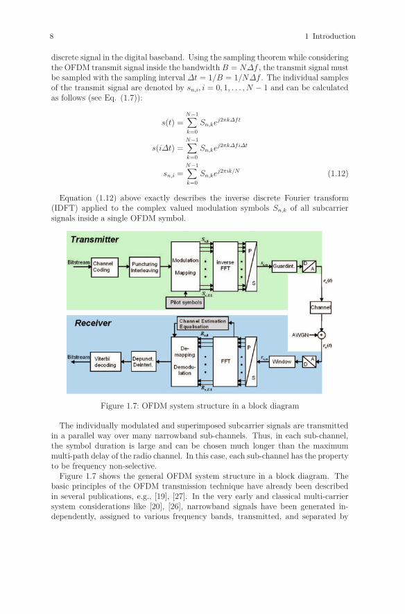
discrete signal in the digital baseband. Using the sampling theorem while consideringthe OFDM transmit signal inside the bandwidth B = NΔf , the transmit signal mustbe sampled with the sampling interval Δt = 1/B = 1/NΔf . The individual samplesof the transmit signal are denoted by sn,i, i = 0, 1, . . . , N − 1 and can be calculatedas follows (see Eq. (1.7)):
s(t) =N−1∑k=0
Sn,kej2πkΔft
s(iΔt) =N−1∑k=0
Sn,kej2πkΔfiΔt
sn,i =N−1∑k=0
Sn,kej2πik/N (1.12)
Equation (1.12) above exactly describes the inverse discrete Fourier transform(IDFT) applied to the complex valued modulation symbols Sn,k of all subcarriersignals inside a single OFDM symbol.
Figure 1.7: OFDM system structure in a block diagram
The individually modulated and superimposed subcarrier signals are transmittedin a parallel way over many narrowband sub-channels. Thus, in each sub-channel,the symbol duration is large and can be chosen much longer than the maximummulti-path delay of the radio channel. In this case, each sub-channel has the propertyto be frequency non-selective.
Figure 1.7 shows the general OFDM system structure in a block diagram. Thebasic principles of the OFDM transmission technique have already been describedin several publications, e.g., [19], [27]. In the very early and classical multi-carriersystem considerations like [20], [26], narrowband signals have been generated in-dependently, assigned to various frequency bands, transmitted, and separated by
1.2 Basics of the OFDM Transmission Technique 9
analog filters at the receiver. The new and modern aspect of the OFDM trans-mission technique is that the various subcarrier signals are generated digitally andjointly by an IFFT in the transmitter and that their spectra strongly overlap onthe frequency axis. As a result, generating the transmit signal is simplified and thebandwidth efficiency of the system is significantly improved.
The received signal is represented by the convolution of the transmitted timesignal with the channel impulse response h(t) and an additive white Gaussian noiseterm:
rn(t) = sn(t) ∗ hn(t) + nn(t) (1.13)
Due to the assumption that the coherence time TC will be much larger thanthe symbol duration TS, the received time-continuous signal rn(t) can be separatedinto the orthogonal subcarrier signal components even in frequency-selective fadingsituations by applying the correlation technique mentioned in Eq. (1.10):
Rn,k =1
TS
∫ TS
0rn(t)e−j2πkΔftdt (1.14)
Equivalently, the correlation process at the receiver side can be applied to the time-discrete receive signal at the output of an A/D converter and can be implementedas a DFT, which leads to Eq. (1.15):
Rn,k =1
N
N−1∑i=0
rn,ie−j2πik/N (1.15)
In this case rn,i = rn(iΔt) describes the i-th sample of the received time-continuousbase-band signal rn(t) and Rn,k is the received complex-valued symbol at the DFToutput of the k-th subcarrier.
If the OFDM symbol duration T is chosen much smaller than the coherence timeTC of the radio channel, the time-variant transfer function of the radio channelH(f, t) can be considered to be constant within the time duration T of each mod-ulation symbol Sn,k for all subcarrier signals. In this case, the effect of the radiochannel in multi-path propagation situations can be described analytically by only asingle multiplication of each subcarrier signal gk(t) with the complex transfer factorHn,k = H(kΔf, nT ). As a result, the received complex valued symbol Rn, k at theDFT output can be described analytically as follows:
rn(t) = sn(t) ∗ hn(t) + nn(t)
rn,i = sn,i ∗ hn,i + nn,i
Rn,k = Sn,k · Hn,k + Nn,k (1.16)
where Nn,k describes an additive noise component for each specific subcarrier gen-erated in the radio channel. Eq. (1.16) shows the most important advantage ofapplying the OFDM transmission technique in practical applications. It encom-passes the complete signal transfer situation of the OFDM block diagram includingIDFT, guard interval, D/A conversion, up- and down-conversion in the RF part,frequency-selective radio channel, A/D conversion and DFT process in the receiver,
10 1 Introduction
neglecting non-ideal behavior of any system components.The transmitted Symbol Sn,k can be recovered, calculating the quotient of the
received complex valued symbol and the estimated channel transfer factor Hn,k:
Sn,k =Rn,k − Nn,k
Hn,k, Sn,k = Rn,k
1
Hn,k
(1.17)
It is obvious that this one tap equalization step of the received signal is much easiercompared to a single carrier system for high data rate applications. The necessaryIDFT and DFT calculations can be implemented very efficiently using the Fast-Fourier-Transform (FFT) Algorithms such as Radix 2, which reduces the systemand computation complexity even more. It should be pointed out that especially thefrequency synchronization at the receiver must be very precise in order to avoid anyInter Carrier Interferences (ICI). Algorithms for time and frequency synchronizationin OFDM based systems will be described in a later chapter of this book.
Besides the complexity aspects, another advantage of the OFDM technique lies inits high degree of flexibility and adaptivity. Division of the available bandwidth intomany frequency-nonselective subbands gives additional advantages for the OFDMtransmission technique. It allows a subcarrier-specific adaptation of transmit pa-rameters, such as modulation scheme (PHY mode) and transmit power (e.g., WaterFilling) in accordance to the observed and measured radio channel status. In a multi-user environment the OFDM structure offers additionally an increased flexibility forresource allocation procedures as compared to SC systems [21]. The importantsystem behavior that all subcarrier signals are mutually orthogonal in the receivermakes the signal processing and the equalization process realized by a single tapprocedure very simple and leads to a low computation complexity.
1.3 OFDM Combined with Multiple Access
Schemes
A very high degree of flexibility and adaptivity is required for new mobile commu-nication systems and for the 4G air interface. The combination between multipleaccess schemes and OFDM transmission technique is an important factor in thisrespect. In principle, multiple access schemes for the OFDM transmission techniquecan be categorized according to OFDM-FDMA, OFDM-TDMA, OFDM-CDMA andOFDM-SDMA [1] [22]. Clearly, hybrid schemes can be applied which are based ona combination of the above techniques. The principles of these basic multiple accessschemes are summarized in Fig. 1.8, where the time-frequency plane is depicted andthe user specific resource allocation is distinguished by different colors.
These access schemes provide a great variety of possibilities for a flexible user spe-cific resource allocation. In the following, one example for OFDM-FDMA is brieflysketched (cf. [7]). In the case that the magnitude of the channel transfer functionis known for each user the subcarrier selection for an OFDM-FDMA scheme can beprocessed in the BS for each user individually which leads to a multi user diversity(MUD) effect. By allocating a subset of all subcarriers with the highest SNR to eachuser the system performance can be improved. This allocation technique based on

1.3 OFDM Combined with Multiple Access Schemes 11
Time
Su
bcarr
iers
Code,
Spac
e
FDMAFDMA TDMATDMA CDMA, SDMACDMA, SDMA
Time
Su
bcarr
iers
Code,
Spac
e
Code,
Spac
e
FDMAFDMA TDMATDMA CDMA, SDMACDMA, SDMA
Figure 1.8: OFDM transmission technique and some multiple access schemes
the knowledge of the channel transfer function shows a large performance advan-tage and a gain in Quality of Service (QoS). Nearly the same flexibility in resourceallocation is possible in OFDM-CDMA systems. But in this case the code orthog-onality is destroyed by the frequency-selective radio channel resulting in multipleaccess interferences (MAI), which reduces the system performance.
Bibliography
[1] R. Grünheid, H. Rohling, “Performance comparison of different multiple accessschemes for the downlink of an ofdm communication system,” In Proc. IEEEVTC, 1997.
[2] T. May, H. Rohling, V. Engels, “Performance Analysis of 64-DAPSK and 64-QAM Modulated OFDM Signals,” IEEE Transactions on Communications,Vol. 46, No. 2, Feb. 1998 pp. 182 - 190.
[3] H. Rohling, R. Grünheid, T. May, K. Brüninghaus, “Digital Amplitude Mod-ulation,” Encyclopedia of Electrical and Electronics Engineering, John Wileyand Sons 1999.
[4] H. Rohling, T. May, K. Brüninghaus, R. Grünheid, “Broad-Band OFDM RadioTransmission for Multimedia Applications,” Proceedings of the IEEE, Vol. 87,No. 10, Oct 1999.
[5] B. Chen, R. Grünheid, H. Rohling, “Scheduling Policies for Joint Optimizationof DLC and Physical Layer in Mobile Communication Systems,” Proc. of the13th IEEE International Symposium on Personal, Indoor and Mobile RadioCommunications (PIMRC 2002), Lisbon, Portugal, September 2002.
[6] R. Grünheid, H. Rohling, J. Ran, E. Bolinth, R. Kern, “Robust Channel Es-timation in Wireless LANs for Mobile Environments,” Proc. VTC 2002 Fall,Vancouver, September 2002.
[7] E. Costa, H. Haas, E. Schulz, D. Galda, H. Rohling, “A low complexity trans-mitter structure for the OFDM-FDMA uplink,” In Proc. IEEE VTC, 2002.
12 1 Introduction
[8] M. Lampe, T. Giebel, H. Rohling, W. Zirwas, “PER Prediction for PHY ModeSelection in OFDM Systems,” Proc. Globecom 2003, San Francisco, USA, De-cember 2003.
[9] M. Lampe, T. Giebel, H. Rohling, W. Zirwas, “Signalling-Free Detection ofAdaptive Modulation in OFDM Systems,” Proc. PIMRC 2003, Peking, China,September 2003.
[10] H. Rohling, D. Galda, “An OFDM based Cellular Single Frequency Communi-cation Network,” Proceedings of WWRF, Beijing, February 23-24, 2004.
[11] H. Rohling, R. Grünheid, “Cross Layer Considerations for an Adaptive OFDM-Based Wireless Communication System,” Wireless Personal Communications,pp. 43 – 57, Springer 2005.
[12] M. Stemick, H. Rohling, “OFDM-FDMA Scheme for the Uplink of a Mo-bile Communication System,” Wireless Personal Communications (2006), June2006.
[13] R. Grünheid, H. Rohling, K. Brüninghaus, U. Schwark, “Self-Organised Beam-forming and Opportunistic Scheduling in an OFDM-based Cellular Network,”Proc. VTC 2006 Spring, Melbourne.
[14] H. Busche, A. Vanaev, H. Rohling, “SVD based MIMO Precoding on Equal-ization Schemes for Realistic Channel Estimation Procedures,” Frequenz 61(2007), 7-8, July/August 2007.
[15] C. Fellenberg, H. Rohling, “Spatial Diversity and Channel Coding Gain ina noncoherent MIMO-OFDM transmission system,” Frequenz Journal of RF-Engineering and Telecommunications, November/December 2008.
[16] C. Fellenberg, H. Rohling, “Quadrature Amplitude Modulation for DifferentialSpace-Time Block Codes,” Wireless Personal Communications, vol. 50, no. 2,pp.247-255, July (II) 2009.
[17] A. Ruiz A. Peled, “Frequency domain data transmission using reduced compu-tational complexity algorithms,” In Proc. IEEE ICASSP, pp. 964-967, 1980.
[18] M. Aldinger, “Multicarrier COFDM scheme in high bitrate radio local areanetworks,” In Proc. Of Wireless Computer Networks, 1994.
[19] P. A. Bello, “Characterization of randomly time-variant linear channels,” IEEETransactions on Communications, Dec. 1964.
[20] R.W. Chang, “Synthesis of band-limited orthogonal signals for multichanneldata transmission,” Bell. Syst. Technical Journal, Vol. 45:pp. 1775–1796, 1966.
[21] L. Hanzo et al, OFDM and MC-CDMA for Broadband Multi-User Communi-cations, WLANs and Broadcasting, Wiley, 2003.

Bibliography 13
[22] S. Kaiser, Multi-Carrier CDMA Mobile Radio Systems - Analysis and Opti-mization of Detection, Decoding and Channel Estimation, VDI-Verlag, 1998.
[23] K. J. R. Liu, A. K. Sadek, W. Su, A. Kwasinski, Cooperative Communicationsand Networking, Cambridge University Press, 2009.
[24] H. Schulze, C. Lueders, Theory and Applications of OFDM and CDMA: Wide-band Wireless Communications, John Wiley and Sons, 2005.
[25] M. Pätzold, Mobile Fading Channels, Wiley, 2002.
[26] B.R. Saltzberg, “Performance of an efficient parallel data transmission system,”IEEE Transactions on Communications, 1967.
[27] P. M. Ebert, S.B. Weinstein, “Data Transmission by Frequency-Division Mul-tiplexing Using the Discrete Fourier Transform,” IEEE Transactions on Com-munication Technology, Vol. Com-19, no. 5, pp. 628–634, 1971.

H. Rohling (ed.), OFDM: Concepts for Future Communication Systems, 15Signals and Communication Technology, DOI: 10.1007/978-3-642-17496-4_2,© Springer-Verlag Berlin Heidelberg 2011
2 Channel Modeling
M. Narandžić, A. Hong, W. Kotterman, R. S. Thomä, Ilmenau Univer-sity of Technology, GermanyL. Reichardt, T. Fügen, T. Zwick, Karlsruhe Institute of Technology(KIT), Germany
In the OFDM signalling concept, the wide-band radio-communication channel iseffectively utilized as a collection of narrow-band channels. Basic system parameterslike the number of subcarriers N and symbol duration T are selected to mitigatethe key channel impairments: Inter-Symbol-Interference (ISI) induced by frequencyselectivity and loss of subcarrier orthogonality due to time selectivity [51]. There-fore, a proper channel model is required both for system design and for performanceevaluation. Additionally, when Channel-State-Information (CSI) is available duringsystem operation, transmission characteristics, such as the signal constellation or theallocated power, could be adaptively adjusted at transmitter per subcarrier in or-der to maximize total throughput. Further improvements of the spectral efficiencycould be obtained by simultaneous transmission and/or reception from/by multi-ple antenna elements. Additionally to time and frequency, this concept known asMIMO (Multiple-Input-Multiple-Output) exploits the spatial propagation dimensionor, more specific, multiplicity of energy propagation paths. Since the reachable spec-tral efficiency is tightly related to the signal correlation across the antenna array [15],the proper representation of correlation levels becomes essential for the analysis ofMIMO systems. In order to obtain an antenna-independent representation of thechannel that implicitly comprises correlation properties, geometry-based models aregenerally used.
In this chapter, the necessary concepts for representation of the multidimensionalradio-channel are summarized. Data collected during multidimensional channelsounding and post-processed by high-resolution parameter estimation algorithms of-fer the most detailed insight into radio-propagation mechanisms. In that way, jointspace-time-frequency representations being consistent with measurements can be ob-tained (Section 2.1). On the other hand, when an appropriate description of the EMenvironment is available (in the form of databases defining geometry and materialproperties), the EM field could be predicted by use of the Geometrical or UniformTheory of Diffraction (GTD/UTD), as explained in Section 2.2. Note that for tuningand verification of ray tracing/launching procedures, sounding experiments are stillrequired. For system design and performance evaluation, site-independent modelingwith lower complexity is preferred. For this purpose, stochastic characterization ofdifferent radio-environment classes could be combined with geometry based propa-gation aspects. This results in the class of Geometry-based Stochastic (GbS) channelmodels that are described in Section 2.3. In order to properly reproduce space-timechannel evolution, this class of empirical models uses stochastic characterization of
16 2 Channel Modeling
Large-Scale Parameters (LSPs) as explained in Subsection 2.3.1. The radio channelscorresponding to specific propagation/deployment scenarios are given as examplesof listed general modeling classes. The characteristics of a radio-link that is estab-lished between vehicle and stationary or moving objects, analyzed by ray-tracingtools, are presented in Subsection 2.2.2. Subsection 2.3.2 introduces GbS model forrelay-links, based on a stochastic representation of channel LSPs. Specific aspects ofspatially-distributed transmission corresponding to cooperative downlink are givenin Subsection 2.3.3. Due to some inherent weaknesses regarding the representationof spatio-temporal evolution, so called analytical models were not considered.
2.1 Joint Space-Time-Frequency Representation
The multidimensional channel transfer function can be equivalently expressed usingthe system functions [4] in either faded domains (r-space, t-time, f -frequency) orresolved domains (Ω-directions, ν-Doppler shift, τ -delay) [27]. The physical modelsbeing discussed here only use resolved domains for channel analysis and synthe-sis, equivalent to characterization by constituent Multi-Path-Components (MPCs).Then, the point-to-point propagation channel (i.e. link) is represented as an antennaresponse to a set of MPCs (usually conveniently grouped into clusters [9], [20]):
H(rT x, rRx, t, f) =∑
i
FTT x(ΩT x
i )αiFRx(ΩRxi )ej2π(τif+νit). (2.1)
Interaction between antennas and MPCs is through the complex, polarimetic an-tenna response
Fr(Ω) = [Fθ(Ω)Fϕ(Ω)]T · ejk(Ω)(r−r0), (2.2)
where Fθ and Fϕ represent projections onto corresponding unitary vectors of thespherical coordinate system. The exponential term in (2.2) defines the phase shiftof MPCs coming from direction Ω w.r.t. the phase center at r0. The given repre-sentation covers all spatial degrees of freedom: transversal movement and antennarotation, as well as any array geometry for the MIMO case. A single MPC corre-sponds to a homogeneous plane wave that within narrow frequency bandwidth canbe characterized by the following parameters:
p = [ΩT x, ΩRx,α, τ, ν], (2.3)
where ΩT and ΩR describe Directions-of-Departure (DoD) and Arrival (DoA),respectively. Due to the inability (in the general case) to represent the Power-Directional-Spectrum as a product of marginal spectra on departure and arrival,joint characterization of DoD and DoA is to be used - as suggested by the double-directional modeling concept [50], [38]. The complex 2-by-2 matrix α ∈ C2×2 is usedto jointly describe MPC magnitude, MPC phase, and cross-polarization effects.
The necessary parameters, normally for a large number of MPCs, could be esti-mated from appropriate multidimensional channel sounding data. These data aregathered during wide-band measurement experiments with specially designed an-tenna arrays and real-time channel sounding devices [49], [26], [7], [8].
2.1 Joint Space-Time-Frequency Representation 17
2.1.1 Multidimensional Channel Sounding
In a broader sense, multidimensional sounding comprises investigations into thespatio-temporal structure of a radio channel, aiming to resolve not only the tempo-ral delay of incoming waves (signal components) but also their angular directionsat transmission and at reception as well as their polarizations. Especially the com-bination of angular resolution and polarimetric state is potentially very costly andlaborious to record and process at its full extent. Many antenna elements are neces-sary for high-resolution results, both to fully cover the angular domain and to createthe required apertures. Providing coverage in a particular direction demands thatantenna elements still have sufficient sensitivity in that direction. Aperture, requiredfor resolution, means that (sensitive) elements are to be spread over space. A popu-lar shortcut like using single-polarized antenna elements leads to biased results [32].Additionally, for accurate parameter estimation, calibration of every antenna ele-ment in the measurement array is mandatory, providing complex radiation patternFr(Ω) of (2.2), required to estimate parameters of resolved MPCs in (2.1), in orderto relate these to observed faded dimensions. Restricting Ω to the azimuthal cut,another popular saving, also means to risk grossly distorted estimates [32].
Characterization of propagation delay requires nearly instantaneous measure-ments, meaning the time needed for a measurement over bandwidth or over thefull delay span should be considerably shorter than the time it takes the channel tochange. Pseudo-random noise sequences, multi-sine tone bursts, or fast frequency-sweeps can be used, each with its own advantages and disadvantages. If the repeti-tion rate is high enough, also the Doppler spectrum or time variability can be deter-mined without aliasing. The temporal and spatial dimension have to be measuredjointly, but measuring all antenna elements simultaneously and all transmit-receivecombinations in parallel is deemed technically infeasible (exception: the 16×4 paral-lel sounding in [41]). Therefore, the antenna combinations are multiplexed, makinguse of one and the same temporal sounding unit. The multiplexing units themselvesare still a technical challenge, due to requirements on switching speed, dampinglosses, feed-through, frequency transfer, delay, and power handling (especially on thetransmit side). Seen these imperfections, the multiplexing units should be calibratedtoo. Synchronization of transmit and receive side, which are often too far apart forsynchronization through a cable connection, requires two free-running clocks of veryhigh stability; typically Rubidium or Cesium standards.
So, what is needed? A dedicated channel sounder with calibrated dedicated multi-plexing equipment both at transmit and receive side, calibrated dedicated antennas,stable (atomic) clocks, and a high-speed data logger. As an example for the latter,the COST2100 urban reference scenario “Ilmenau” had to be measured at a mod-est trawling speed of 3 m/s, in order not to exceed the maximum sustained datatransfer rate of 1.2 Gbit/s, the product of snapshot rate, number of transmit-receivecombinations, impulse response length, and number of bits per time sample [48].
2.1.2 Extraction of Parameters for Dominant MPCs
The estimation procedure of MPC parameters from channel sounding data requiresthe use of so called high-resolution algorithms , like, e.g., Maximum Likelihood

18 2 Channel Modeling
Estimation [60], ESPRIT (Estimation of Signal Parameters via Rotational Invari-ance Techniques) [44], [52], SAGE (Space-Alternating Generalized Expectation-maximization) [14], or RIMAX [53], [46], [32]. An alternative to measurementsis the extraction of model parameters by means of ray tracing (Section 2.2).
Both methods could provide reliable (reality matching) parameters for only a lim-ited number of MPCs: the measurement-based estimation due to the limited numberof space-time-frequency observations [46] and the limited precision of antenna cali-bration [32], and ray-tracing due to the limited precision of the radio-environmentmodel. The remaining part, usually associated with diffuse scattering, is typicallycharacterized by stochastic means both during parameter estimation [46], [32] andray generation [10].
2.2 Deterministic Modeling
Deterministic models are used for site-specific channel modeling; they consist ofan environment model and a wave propagation model. The environment modeldescribes position, geometry, material composition and surface properties of thewave propagation relevant objects and obstacles (e.g. trees, houses, vehicles, walls,etc.). The well-known Maxwell equations [3] always form the basis for all investi-gations of electromagnetic fields. In practical applications an analytic solution ofthe Maxwell equations, due to the computation time, is not possible. Also numericapproximation methods, like, e.g., the Parabolic Equation Method (PEM) or theFinite Difference Time Domain Method (FDTD) [21], [57], [59] fail for efficiencyreasons with problems, which are larger than some wavelengths in the examinedfrequency range. Substantially less complexity and computing time is achievablewith geometric-optical models [30], [5], [56], [2], [25], [35], [17], [16]. These modelsare based on iterated approaches, which use the border behavior of electromagneticfields for high frequencies [37]. The use of these procedures makes substantial simpli-fications of the description of the wave propagation possible. This allows to computeelectrically very large problems very efficient and exactly.
2.2.1 Relevant GTD/UTD Aspects
The modern geometrical optics (GO) is an important representative of these iteratedprocedures, and it forms the basis for the uniform geometrical theory of diffraction(UTD). The validity of the GO does not alone depend on the frequency. A furthercondition is, that the scattering objects contained in the propagation vicinity arelarge in relation to the wavelength. Additionally the surface texture is not allowedto change over a wavelength. Further the material properties of the propagationmedium must be constant within the range of a wavelength [37]. This is fulfilled ingood approximation for frequencies above 1 GHz.
Due to its flexibility and accuracy geometric-optical models are already today inuse. They are able to calculate, a place-dependent prognosis of the full-polarimetricfield strength and/or receiving power in the regarded propagation area. Besides thisa complete narrow- and wide-band description of the mobile channel is possible, whythey find increased use in system simulations [12], [36].

2.2 Deterministic Modeling 19
Figure 2.1: With Ray-tracing calculated wave propagation in a high-speed train sce-nario [29].
2.2.2 Vechicle2X Channel Modeling
The realistic channel representation at very high participant velocities in combina-tion with high data rate transmission and MIMO-OFDM techniques can be obtainedby a ray-optical description of the multi-path propagation. In the context of the keyprogram TakeOFDM of the Deutsche Forschungsgesellschaft (DFG) such a channelmodel for high-speed train communication was developed (Fig. 2.1) [29]. A detaileddescription of the vehicle’s vicinity is essential for a proper modeling of the wavepropagation. This includes the track, on which the vehicles are driving, and theenvironment adjacent to the track. E.g. in the surrounding of train tracks possibleobjects are noise barriers, trees, signs, bridges, and pylons, whereas in urban or sub-urban areas buildings are more probable. A new map generator has been developedfor this ray-tracing simulator. With this, it is possible to import standard CAD(Computer Aided Design) data with the STL (Standard Triangulation Language)format. In the map generator the electrical parameters like the permittivity εr, per-meability μr and the standard deviation of the surface roughness σ are assigned tothe objects and it is possible to shift, scale or rotate them. Furthermore it is possibleto define velocities for the objects to create a time series of snapshots of the scenarioto simulate the time-variant behavior of the channel. For the channel simulationseach object can be equipped with a receiver and a transmitter. The position ofthe corresponding antennas as well as the antenna pattern and orientation can bechosen arbitrarily. An accurate description of the multi-path wave propagation inthe aforementioned scenarios is required to produce realistic time series of ChannelImpulse Responses (CIRs).
At the Institut für Hochfrequenztechnik und Elektronik a three-dimensional ray-tracing algorithm has been developed and implemented [36]. The results of theapplied ray tracing algorithms have been verified by measurements in different sce-
20 2 Channel Modeling
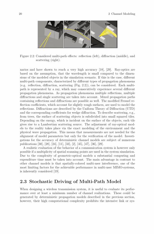
Figure 2.2: Considered multi-path effects: reflection (left), diffraction (middle), andscattering (right).
narios and have shown to reach a very high accuracy [18], [29]. Ray-optics arebased on the assumption, that the wavelength is small compared to the dimen-sions of the modeled objects in the simulation scenario. If this is the case, differentmulti-path components, characterized by different types of propagation phenomena(e.g. reflection, diffraction, scattering (Fig. 2.2)), can be considered. Each multi-path is represented by a ray, which may consecutively experience several differentpropagation phenomena. As propagation phenomena multiple reflections, multiplediffractions and single scattering are taken into account. Mixed propagation pathscontaining reflections and diffractions are possible as well. The modified Fresnel re-flection coefficients, which account for slightly rough surfaces, are used to model thereflections. Diffractions are described by the Uniform Theory of Diffraction (UTD)and the corresponding coefficients for wedge diffraction. To describe scattering, e.g.,from trees, the surface of scattering objects is subdivided into small squared tiles.Depending on the energy, which is incident on the surface of the objects, each tilegives rise to a Lambertian scattering source. The adjustment of ray-optical mod-els to the reality takes place via the exact modeling of the environment and thephysical wave propagation. This means that measurements are not needed for thealignment of model parameters but only for the verification of the model. Investi-gations for the accuracy of deterministic channel models are subject of numerouspublications [30], [28], [24], [11], [33], [2], [45], [47], [36], [29].
A realistic evaluation of the behavior of a communication system is however onlypossible if a multiplicity of spatial scanning points are used in the system simulation.Due to the complexity of geometric-optical models a substantial computing andexpenditure time must be taken into account. The main advantage in contrast toother channel models is that spatially-colored multi-user interference, one of themost limiting factors for the achievable performance in multi-user MIMO-systems,is inherently considered [19].
2.3 Stochastic Driving of Multi-Path Model
When designing a wireless transmission system, it is useful to evaluate its perfor-mance over at least a minimum number of channel realizations. These could begenerated by deterministic propagation models described in the previous section,however, their high computational complexity prohibits the intensive link or sys-
2.3 Stochastic Driving of Multi-Path Model 21
tem level simulations required during system design. Thus, procedures with a lowercomputational complexity that could emulate a whole class of radio-propagationenvironments (i.e. propagation scenario) are preferred. These requirements haveled to the Geometry-based Stochastic (GbS) channel models where generated multi-path components are not directly related to any particular (or very detailed) radio-environment. Instead, the channel realizations are determined as realizations of amultidimensional random process that characterizes all aspect of physical plane-wavepropagation.
The stochastic generation of multipath can be done in several different forms. Wewould distinguish two classes according to the use of the scattering (or interacting)objects during the physical model synthesis. E.g. it is possible to place interactingobjects in a 2D/3D coordinating system, and to perform their abstraction in theform of multipath clusters as in the COST 273 model [8]. By assigning visibilityregions [1] to each of the clusters, a simplified ray-tracing engine is obtained. Therandomness in this approach is attained by random selection of visibility regions andthe intra-cluster structure. An alternative would be to fully remove scatterers fromthe model synthesis. In this case multipath components are no longer related toparticular scatterers, but are generated in the so called parametric domain instead.This term relates to the parameters of multipath components as given by (2.3).Typical representatives are the 3GPP Spatial-Channel-Model [54], the channel modeldeveloped in the WINNER project [31], and the reference model for evaluation ofIMT-Advanced radio interface technologies [34].
2.3.1 Usage of the Large-Scale Parameters for ChannelCharacterization
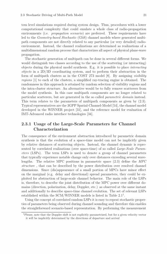
The consequence of the environment abstraction introduced by parametric domainsynthesis is that the evolution of a space-time model can not be implicitly givenby relative distances of scattering objects. Instead, the channel dynamic is repre-sented by correlated realizations (over space-time) of so called Large-Scale Param-eters (LSPs). The term LSPs is used to denote a group of channel parametersthat typically experience notable change only over distances exceeding several wave-lengths. The relative MPC positions in parametric space (2.3) define the MPCstructure , that can be described by the power distribution over resolved channeldimensions. Since (dis)appearance of a small portion of MPCs have minor effecton the marginal (e.g. delay and directional) spread parameters, they could be ex-ploited for abstraction of large-scale channel behavior. The main role of the LSPsis, therefore, to describe the joint distribution of the MPC power over different do-mains (direction, polarization, delay, Doppler, etc.) as observed at the same instantand additionally to describe space-time channel evolution. The set of relevant LSPsestablished within the SCM/WINNER models is listed in Table 2.11.
Using the concept of correlated random LSPs it is easy to repeat stochastic proper-ties of parameters being observed during channel sounding and therefore this enablesthe straightforward scenario-based representation. By performing the measurement
1Please, note that the Doppler shift is not explicitly parametrized, but for a given velocity vectorit will be implicitly determined by the directions of departure and arrival
22 2 Channel Modeling
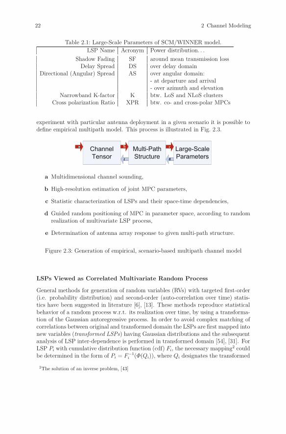
Table 2.1: Large-Scale Parameters of SCM/WINNER model.LSP Name Acronym Power distribution. . .
Shadow Fading SF around mean transmission lossDelay Spread DS over delay domain
Directional (Angular) Spread AS over angular domain:- at departure and arrival- over azimuth and elevation
Narrowband K-factor K btw. LoS and NLoS clustersCross polarization Ratio XPR btw. co- and cross-polar MPCs
experiment with particular antenna deployment in a given scenario it is possible todefine empirical multipath model. This process is illustrated in Fig. 2.3.
a Multidimensional channel sounding,
b High-resolution estimation of joint MPC parameters,
c Statistic characterization of LSPs and their space-time dependencies,
d Guided random positioning of MPC in parameter space, according to randomrealization of multivariate LSP process,
e Determination of antenna array response to given multi-path structure.
Figure 2.3: Generation of empirical, scenario-based multipath channel model
LSPs Viewed as Correlated Multivariate Random Process
General methods for generation of random variables (RVs) with targeted first-order(i.e. probability distribution) and second-order (auto-correlation over time) statis-tics have been suggested in literature [6], [13]. These methods reproduce statisticalbehavior of a random process w.r.t. its realization over time, by using a transforma-tion of the Gaussian autoregressive process. In order to avoid complex matching ofcorrelations between original and transformed domain the LSPs are first mapped intonew variables (transformed LSPs) having Gaussian distributions and the subsequentanalysis of LSP inter-dependence is performed in transformed domain [54], [31]. ForLSP Pi with cumulative distribution function (cdf) Fi, the necessary mapping2 couldbe determined in the form of Pi = F−1
i (Φ(Qi)), where Qi designates the transformed
2The solution of an inverse problem, [43]
2.3 Stochastic Driving of Multi-Path Model 23
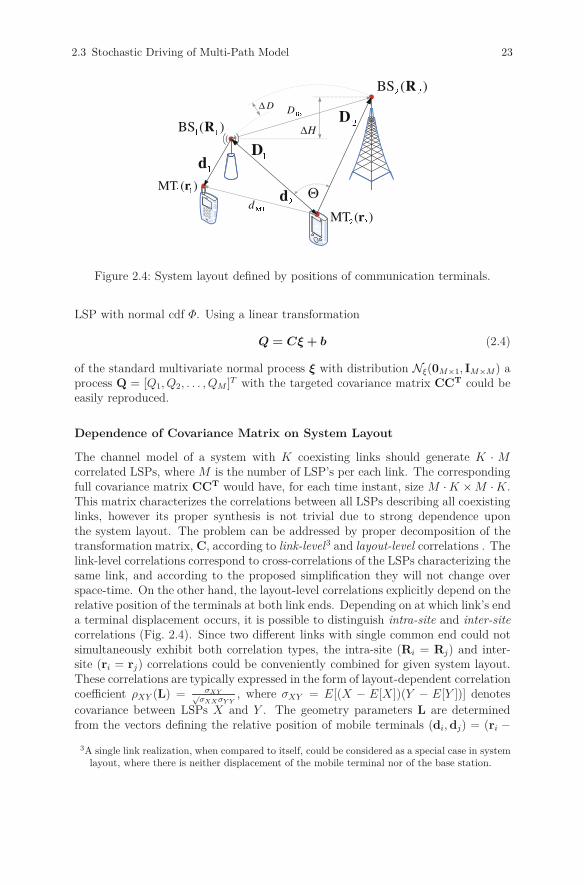
Figure 2.4: System layout defined by positions of communication terminals.
LSP with normal cdf Φ. Using a linear transformation
Q = Cξ+ b (2.4)
of the standard multivariate normal process ξ with distribution Nξ(0M×1, IM×M) aprocess Q = [Q1, Q2, . . . , QM ]T with the targeted covariance matrix CCT could beeasily reproduced.
Dependence of Covariance Matrix on System Layout
The channel model of a system with K coexisting links should generate K · Mcorrelated LSPs, where M is the number of LSP’s per each link. The correspondingfull covariance matrix CCT would have, for each time instant, size M · K × M · K.This matrix characterizes the correlations between all LSPs describing all coexistinglinks, however its proper synthesis is not trivial due to strong dependence uponthe system layout. The problem can be addressed by proper decomposition of thetransformation matrix, C, according to link-level3 and layout-level correlations . Thelink-level correlations correspond to cross-correlations of the LSPs characterizing thesame link, and according to the proposed simplification they will not change overspace-time. On the other hand, the layout-level correlations explicitly depend on therelative position of the terminals at both link ends. Depending on at which link’s enda terminal displacement occurs, it is possible to distinguish intra-site and inter-sitecorrelations (Fig. 2.4). Since two different links with single common end could notsimultaneously exhibit both correlation types, the intra-site (Ri = Rj) and inter-site (ri = rj) correlations could be conveniently combined for given system layout.These correlations are typically expressed in the form of layout-dependent correlationcoefficient ρXY (L) = σXY√
σXXσY Y, where σXY = E[(X − E[X])(Y − E[Y ])] denotes
covariance between LSPs X and Y . The geometry parameters L are determinedfrom the vectors defining the relative position of mobile terminals (di, dj) = (ri −
3A single link realization, when compared to itself, could be considered as a special case in systemlayout, where there is neither displacement of the mobile terminal nor of the base station.

24 2 Channel Modeling
R, rj − R) or base stations (Di, Dj) = (Ri − r, Rj − r) w.r.t. to single commonposition (Fig. 2.4). The set of relevant parameters L for intra-site correlations couldbe reduced to Euclidean distance between mobile terminals dMT = ||ri − rj|| [31].The characterization of inter-site correlations , however, requires a more complexparameter space L = [Θ, ΔD, DBS, ΔH]T [40] being defined at Fig. 2.4.
2.3.2 Relaying
In wireless communication systems, the nodes with a relaying capability are inte-grated into conventional networks in order to provide a ubiquitous coverage withhigh data rates, especially in the areas with a high shadowing [42]. In relay net-works, intermediate Relay-Stations (RSs) are introduced into the communicationbetween a base station and a mobile terminal. If station labeled as BS1 has re-lay functionality, than the Fig. 2.4 can be interpreted as an example of the basicthree-station structured relay network [55]. The purpose of intermediate RS (BS1)would be to forward received signals from BS2 toward mobile terminal MT1, andvice versa [58]. The introduction of intermediate RSs results in a meshed topologyof relay networks, and brings new challenges in channel modeling. Moreover, char-acterizing and modeling of the relationship between meshed links, is one of the mostcrucial points in the channel modeling of relay networks . The correlation proper-ties between meshed links can be captured in the form of the intra- and inter-sitecorrelations of large scale parameters [22], as discussed in previous subsection. Theobserved correlation properties for relay measurements in Ilmenau inner city, couldbe summarized as follows [23]:
1. The de-correlation distance (used to characterize intra-site correlations) of SF,DS as well as XPR decrease with a reduced BS height. This confirms thateven the intra-site correlation could exhibit more complex layout dependence.
2. The inter-site correlation of LSPs is high when two BSs/RSs are near to eachother but a MT is far away from both.
3. The larger the difference in the height of two BSs/RSs, the lower the inter-sitecorrelation.
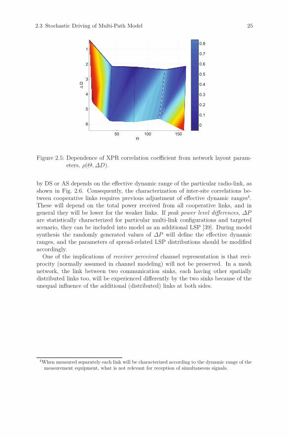
4. The inter-site correlation decreases for larger angular separation of BSs, Θ.Figure 2.5 shows the experimental results for inter-site correlation coefficientof XPR. Note, that measured correlation does not decrease monotonicallyneither with angular nor distance separation ΔD.
2.3.3 Cooperative Downlink
One of the main goals behind the physical modeling is to make the channel represen-tation as independent from the system aspects as possible. However, when charac-terizing the cooperative downlink (e.g. (−D1, −D2) from Fig. 2.4) it is not possibleto disregard the influence of the receiver’s limited dynamic range on perceived LSPsof the cooperative links [39]. Namely, the perception of power spreading expressed
2.3 Stochastic Driving of Multi-Path Model 25
50 100 150
6
5
4
3
2
1
Θ
Δ D
0
0.1
0.2
0.3
0.4
0.5
0.6
0.7
0.8
Figure 2.5: Dependence of XPR correlation coefficient from network layout param-eters, ρ(Θ, ΔD).
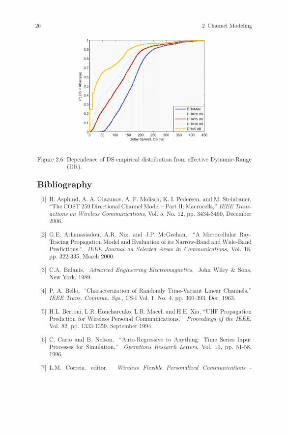
by DS or AS depends on the effective dynamic range of the particular radio-link, asshown in Fig. 2.6. Consequently, the characterization of inter-site correlations be-tween cooperative links requires previous adjustment of effective dynamic ranges4.These will depend on the total power received from all cooperative links, and ingeneral they will be lower for the weaker links. If peak power level differences, ΔPare statistically characterized for particular multi-link configurations and targetedscenario, they can be included into model as an additional LSP [39]. During modelsynthesis the randomly generated values of ΔP will define the effective dynamicranges, and the parameters of spread-related LSP distributions should be modifiedaccordingly.
One of the implications of receiver perceived channel representation is that reci-procity (normally assumed in channel modeling) will not be preserved. In a meshnetwork, the link between two communication sinks, each having other spatiallydistributed links too, will be experienced differently by the two sinks because of theunequal influence of the additional (distributed) links at both sides.
4When measured separately each link will be characterized according to the dynamic range of themeasurement equipment, what is not relevant for reception of simultaneous signals.
26 2 Channel Modeling
0 50 100 150 200 250 300 350 400 4500
0.1
0.2
0.3
0.4
0.5
0.6
0.7
0.8
0.9
1
Delay Spread, DS [ns]
P( D
S <
Abs
ciss
a)
DR=MaxDR=20 dBDR=15 dBDR=10 dBDR=5 dB
Figure 2.6: Dependence of DS empirical distribution from effective Dynamic-Range(DR).
Bibliography
[1] H. Asplund, A. A. Glazunov, A. F. Molisch, K. I. Pedersen, and M. Steinbauer,“The COST 259 Directional Channel Model – Part II: Macrocells,” IEEE Trans-actions on Wireless Communications, Vol. 5, No. 12, pp. 3434-3450, December2006.
[2] G.E. Athanasiadou, A.R. Nix, and J.P. McGeehan, “A Microcellular Ray-Tracing Propagation Model and Evaluation of its Narrow-Band and Wide-BandPredictions,” IEEE Journal on Selected Areas in Communications, Vol. 18,pp. 322-335, March 2000.
[3] C.A. Balanis, Advanced Engineering Electromagnetics, John Wiley & Sons,New York, 1989.
[4] P. A. Bello, “Characterization of Randomly Time-Variant Linear Channels,”IEEE Trans. Commun. Sys., CS-I Vol. 1, No. 4, pp. 360-393, Dec. 1963.
[5] H.L. Bertoni, L.R. Honcharenko, L.R. Macel, and H.H. Xia, “UHF PropagationPrediction for Wireless Personal Communications,” Proceedings of the IEEE,Vol. 82, pp. 1333-1359, September 1994.
[6] C. Cario and B. Nelson, “Auto-Regressive to Anything: Time Series InputProcesses for Simulation,” Operations Research Letters, Vol. 19, pp. 51-58,1996.
[7] L.M. Correia, editor, Wireless Flexible Personalized Communications -
Bibliography 27
COST259: European Commission in Mobile Radio Research, Wiley, New York,2001.
[8] L.M. Correia, editor, Mobile Broadband Multimedia Networks - Techniques,Models and Tools for 4G, COST 273 Final Report, Elsevier, Oxford, 2006.
[9] N. Czink, The Random-Cluster Model, PhD thesis, Technische UniversitätWien, 2007.
[10] D. Didascalou, M. Döttling, N. Geng, and W. Wiesbeck, “An Approach toInclude Stochastic Rough Surface Scattering into Deterministic Ray-OpticalWave Propagation Modeling,” IEEE Transactions on Antennas and Propaga-tion, Vol. 51, No. 7, pp. 1508–1515, July 2003.
[11] D.L. Didascalou, Ray-Optical Wave Propagation in Arbitrarily Shaped Tunnels,PhD thesis, Forschungsberichte aus dem Institut für Höchstfrequenztechnik undElektronik der Universität Karlsruhe (TH), 2000.
[12] M.W. Döttling, Strahlenoptisches Wellenausbreitungsmodell und Systemstudienfür den Sattelitenmobilfunk, PhD thesis, Forschungsberichte aus dem Insti-tut für Höchstfrequenztechnik und Elektronik der Universität Karlsruhe (TH),Karlsruhe, Germany, 2000.
[13] S. Fitzgerald, J. Placeb, and A. van de Liefvoort, “Generating correlated matrixexponential random variables,” Advances in Engineering Software, Vol. 37,pp. 75-84, 2006.
[14] B.H. Fleury, M. Tschudin, R. Heddergott, D. Dahlhaus, and K. Ingeman Ped-ersen, “Channel Parameter Estimation in Mobile Radio Environments usingthe SAGE Algorithm,” IEEE Journal on Selected Areas in Communications,Vol. 17, No. 3, pp. 434-450, March 1999.
[15] G. J. Forschini and M. J. Gans, “On limits of wireless communications in afading environment when using multiple antennas,” Wireless Personal Com-munications, Vol. 6, No. 3, pp. 311-335, 1998.
[16] T. Fügen, Richtungsaufgelöste Kanalmodellierung und Systemstudien fürMehrantennensysteme in urbanen Gebieten , PhD thesis, Universität Karl-sruhe, Karlsruhe, Germany, 2009.
[17] T. Fügen, J. Maurer, T. Kayser, and W. Wiesbeck, “Capability of 3D Ray Trac-ing for Defining Parameter Sets for the Specification of Future Mobile Commu-nications Systems,” IEEE Transactions on Antennas and Propagation, SpecialIssue on Wireless Communications, Vol. 54, No. 11, pp. 3125-3137, November2006.
[18] T. Fügen, J. Maurer, T. Kayser, and W. Wiesbeck, “Verification of 3D Ray-tracing with Non-Directional and Directional Measurements in Urban Macro-cellular Environments,” in Proceedings of the 63th IEEE Vehicular TechnologyConference, VTC2006-Spring, Melbourne, Australia, May 2006.
28 2 Channel Modeling
[19] T. Fügen, J. Maurer, C. Kuhnert, and W. Wiesbeck, “A Modelling Approach forMultiuser MIMO Systems Including Spatially-Colored Interference,” in Proceed-ings of the IEEE Global Telecommunications Conference, GLOBECOM 2004,Vol. 2, pp. 938-942, Dallas, TX, December 2004.
[20] T. Fügen, J. Maurer, W. Sörgel, and W. Wiesbeck, Characterization of Mul-tipath Clusters with Ray-Tracing in Urban MIMO Propagation Environmentsat 2 GHz. in IEEE International Symposium on Antennas and Propagation,Vol. 3B, pp. 410-413, Washington DC, USA, July 2005.
[21] N. Geng, Modellierung der Ausbreitung elektromagnetischer Wellen in Funksys-temen durch Lösung der parabolischen Approximation der Helmholtz-Gleichung,PhD thesis, Forschungsberichte aus dem Institut für Höchstfrequenztechnik undElektronik der Universität Karlsruhe (TH), 1996.
[22] A. Hong, M. Narandžić, C. Schneider, and R. S. Thomä, “Estimation of theCorrelation Properties of Large Scale Parameters from Measurement Data,” inIEEE International Symposium on Personal, Indoor and Mobile Radio Com-munications (PIMRC), Athens, Greece, Sep. 2007.
[23] A. Hong and R. S. Thomä, “Experimental Study on the Impact of the Base Sta-tion Height on the Channel Parameters,” in ITG Workshop on Smart Antennas,Berlin, Germany, Feb. 2009.
[24] R. Hoppe, G. Wölfle, and F.M. Landstorfer, “Accelerated Ray Optical Prop-agation Modeling for the Planning of Wireless Communication Networks,” inProceedings of the IEEE Radio and Wireless Conference, RAWCON 99, pp. 159-162, Denver, CO, USA, August 1999.
[25] M.F. Iskander and Z. Yun, “Propagation Prediction Models for Wireless Com-munication Systems,”, IEEE Transactions on Microwave Theory and Tech-niques, Vol. 50, pp. 662-673, March 2002.
[26] M.A. Jensen and J.W. Wallace, “MIMO Wireless Channel Modeling and Exper-imental Characterization,” in A.B. Gershman and N.D. Sidiropoulos, editors,Space-Time Signal Processing for MIMO Communications, pp. 1-39. John Wi-ley & Sons, 2005.
[27] R. Kattenbach, “Statistical Modeling of Small-Scale Fading in Directional RadioChannels,” IEEE J. Select. Areas Communications, Vol. 20, pp. 584-592, Apr.2002.
[28] Seong-Cheol Kim, B.J. Jr. Guarino, T.M. III Willis, V. Erceg, S.J. Fortune,R.A. Valenzuela, L.W. Thomas, J. Ling, and J.D. Moore, “Radio PropagationMeasurements and Prediction Using Three-Dimensional Ray Tracing in UrbanEnvironments at 908 MHz and 1.9 GHz,” IEEE Transactions on VehicularTechnology, Vol. 48, No. 3, pp. 931-946, May 1999.

Bibliography 29
[29] S. Knörzer, Funkkanalmodellierung für OFDM-Kommunikation beiHochgeschwindigkeitszügen, PhD thesis, Universität Karlsruhe, Karlsruhe, Ger-many, 2009.
[30] T. Kürner, D.J. Cichon, and W. Wiesbeck, “Concepts and Results for 3DDigital Terrain-Based Wave Propagation Models: An Overview,” IEEE Journalon Selected Areas in Communications, Vol. 11,pp. 1002-1012, September 1993.
[31] P. Kyösti, J. Meinilä, L. Hentilä, X. Zhao, T. Jämsä, C. Schneider, M.Narandžić, M. Milojević, A. Hong, J. Ylitalo, V.-M. Holappa, M. Alatossava,R. Bultitude, Y. de Jong, and T. Rautiainen, “IST-4-027756 WINNER IIDeliverable 1.1.2. v.1.2, WINNER II Channel Models,” Technical report, IST-WINNERII, September 2007.
[32] M. Landmann, Limitations of Experimental Channel Characterisation, PhDthesis, Technische Universität Ilmenau, Ilmenau, Germany, March 2008.
[33] H.-J. Li, C.C. Chen, T.-Y. Liu, and H.-C. Lin, “Applicability of Ray-TracingTechnique for the Prediction of Outdoor Channel Characteristics,”. IEEETransactions on Vehicular Technology, Vol. 49, No. 6, pp. 2336-2349, November2000.
[34] ITU-R M.2135, “Guidelines for evaluation of radio interface technologies forimt-advanced,” Technical report, International Telecommunication Union, Ra-diocommunication Sector (ITU-R), 2008.
[35] J. Maurer, Strahlenoptisches Kanalmodell für die Fahrzeug-Fahrzeug-Funkkommunikation, PhD thesis, Forschungsberichte aus dem Institut fürHöchstfrequenztechnik und Elektronik der Universität Karlsruhe (TH), 2005.
[36] J. Maurer, T. Fügen, and W. Wiesbeck, “Physical Layer Simulations ofIEEE802.11a for Vehicle-to-Vehicle Communications,” in Proceedings of the62th IEEE Vehicular Technology Conference, VTC2005-Fall, Vol. 3, pp. 1849-1853, Dallas, TX, September 2005.
[37] D.A. McNamara, C.W.I. Pistorius, and J.A.G. Malherbe, Introduction to theUniform Geometrical Theory of Diffraction, Artech House, Boston, 1990.
[38] A. F. Molisch, H. Asplund, R. Heddergott, M. Steinbauer, and T. Zwick, “TheCOST259 Directional Channel Model – Part I: Overview and Methodology,”.IEEE Transactions on Wireless Communications, Vol. 5, No. 12, pp. 3421-3433,December 2006.
[39] M. Narandžić, W. Kotterman, M. Käske, C. Schneider, G. Sommerkorn,A. Hong, and R. S. Thomä, “On a Characterization of Large-Scale Parametersfor Distributed (Multi-Link) MIMO - the Impact of Power Level Differences,”in European Conference on Antennas and Propagation (EuCAP), Barcelona,Spain, Apr. 2010.
30 2 Channel Modeling
[40] M. Narandžić, P. Kyösti, J. Meinilä, L. Hentilä, M. Alatossava, T. Rautiainen,Y.L.C. de Jong, C. Schneider, and R. S. Thomä, “Advances in WINNERWideband MIMO System-Level Channel Modelling,” in Proc. of the 2nd Eu-ropian Conference on Antennas and Propagation (EUCAP), Edinburgh, UK,Nov. 2007.
[41] J.Ø. Nielsen, J.B. Andersen, P.C.F. Eggers, G.F. Pedersen, K. Olesen,E.H. Sørensen, and H. Suda, “Measurements of Indoor 16×32 Wideband MIMOChannels at 5.8 GHz,” in ISSSTA2004, pp. 864–868, 2004.
[42] R. Pabst et al., “Relay based deployment concepts for wireless and mobilebroadband radio,” IEEE Communication Magazine, Vol. 42, pp. 80-89, Sep.2004.
[43] A. Papoulis, Probability, Random Variables, and Stochastic Processes, Mc-Graw Hill, 3rd edition, 1991.
[44] A.J. Paulraj, R. Roy, and T. Kailath, “Estimation of Signal Parameters via Ro-tational Invariance Techniques - ESPRIT,” in Proceedings of the 19th AsilomarConference on Circuits, Systems and Computers, pp. 83-89, Nov. 1985.
[45] T. Rautiainen, G. Wölfle, and R. Hoppe, “Verifying Path Loss and Delay SpreadPredictions of a 3D Ray Tracing Propagation Model in Urban Environment,” inProceedings of the 56th IEEE Vehicular Technology Conference, VTC2002-Fall,pp. 1264-1268, Vancouver, BC, Canada, September 2002.
[46] A. Richter, Estimation of Radio Channel Parameters: Models and Algorithms,PhD thesis, Technische Universität Ilmenau, Ilmenau, Germany, 2005.
[47] J.-P. Rossi and Y. Gabillet, “A Mixed Ray Launching/Tracing Method forFull 3-D UHF Propagation Modeling and Comparison With Wide-Band Mea-surements,” IEEE Transactions on Antennas and Propagation, Vol. 50, No. 4,pp. 517-523, April 2002.
[48] C. Schneider, G. Sommerkorn, M. Narandžić, M. Käske, A. Hong, V. Algeier,W. Kotterman, R.S. Thomä, and C. Jandura, “Multi-User MIMO ChannelReference Data for Channel Modelling and System Evaluation from Measure-ments,” in International IEEE Workshop on Smart Antennas (WSA 2009),Berlin, Germany, February 2009.
[49] L. Schumacher, L.T Berger, and J. Ramiro-Moreno, “Propagation Characteri-zation and MIMO Channel Modeling for 3G,” in S. Chandran, editor, AdaptiveAntenna Arrays; Trends and Applications, pp. 377-393. Springer, 2004.
[50] M. Steinbauer, A.F. Molisch, and E. Bonek, “The Double-Directional RadioChannel,” IEEE Transactions on Antennas and Propagation, Vol. 43, No. 4,pp. 51-63, August 2001.
[51] G. L. Stüber, “Principles of Mobile Communications,” Kluwer Academic Pub-lishers, 2002.

Bibliography 31
[52] R.S. Thomä, D. Hampicke, A. Richter, G. Sommerkorn, A. Schneider,U. Trautwein, and W. Wirnitzer, “Identification of Time-Variant DirectionalMobile Radio Channels,” IEEE Transactions on Instrumentation and Measure-ment, Vol. 49, No. 2, pp. 357-364, April 2000.
[53] R.S. Thomä, M. Landmann, and A. Richter, “RIMAX - a Maximum LikelihoodFramework for Parameter Estimation in Multidimensional Channel Sounding,”in 2004 International Symposium on Antennas and Propagation, Sendai, Japan,August 2004.
[54] 3GPP TR 25.996 V6.1.0, “Spatial Channel Model for MIMO Simulations,”Technical report, Third Generation Partnership Project (3GPP), Sept. 2003.
[55] E. C. van der Meulen, “Three-Terminal Communication Channels,” Advancesin Applied Probability, Vol. 3, pp. 120-154, 1971.
[56] G.A.J. van Dooren, A Deterministic Approach to the Modelling of Electro-magnetic Wave Propagation in Urban Environments, PhD thesis, University ofEindhoven, The Netherlands, 1994.
[57] Y. Wang, S. Safavi-Naeini, and S.K. Chaudhuri, “A Hybrid Technique Basedon Combining Ray Tracing and FDTD Methods for Site-Specific Modeling ofIndoor Radio Wave Propagation,” IEEE Transactions on Antennas and Prop-agation, Vol. 48, No. 5, pp. 743-753, May 2000.
[58] H. Wijaya, Broadband Multi-Hop Communication in Homogeneous and Hetero-geneous Wireless Lan Networks, PhD thesis, Technische Hochschule Aachen,Germany, Feb. 2005.
[59] K.I. Ziri-Castro, W.G. Scanlon, and N.E. Evans, “Prediction of Variation inMIMO Channel Capacity for the Populated Indoor Environment using a RadarCross-Section-Based Pedestrian Model,”. IEEE Transactions on Wireless Com-munications, Vol. 4, No. 3, pp. 1186-1194, May 2005.
[60] M. Ziskind, I. Wax, “Maximum Likelihood Localization of Multiple Sources byAlternating Projection,” IEEE Transactions on Acoustics, Speech, and SignalProcessing, Vol. 36, pp. 1553-1560, October 1988.


H. Rohling (ed.), OFDM: Concepts for Future Communication Systems, 33Signals and Communication Technology, DOI: 10.1007/978-3-642-17496-4_3,© Springer-Verlag Berlin Heidelberg 2011
3 Link-Level Aspects
3.1 OFDM Data Detection and Channel
Estimation
P. A. Hoeher, University of Kiel, Germany
3.1.1 Introduction
OFDM is a popular multicarrier transmission technique employing orthogonal sub-carriers. It has been successfully applied in data modems, audio and video broad-casting systems, wireless local area networks, cellular radio, and is a suitable can-didate for next generation wireless and wireline systems. Inherent advantages ofOFDM include its ease of implementation (due to FFT processing), its robustnessagainst multipath fading (due to a guard interval/cyclic extension), and its band-width efficiency (due to the ability of adaptive power and bit loading) [1]. Multi-userMIMO systems based on OFDM are currently under intensive investigation. How-ever, the bit error performance degrades if orthogonality can not be maintained.Reasons for this include fast fading, phase jitter, frequency offset, delay spread ex-ceeding the guard interval, and nonlinear distortions. All these effects cause crosstalkbetween the subcarriers. In contrast to multicarrier transmission techniques withnon-orthogonal subcarrier signals (such as multicarrier systems with Gaussian pulseshaping), all subcarriers interfere with each other. The problems are especially se-vere in the presence of a “dirty RF” receiver design [2]. As a consequence, optimumreception is prohibitive if orthogonality is lost. Particularly challenging are issue likedata detection, channel estimation, and synchronization. These topics have been ad-dressed in our working group. In this chapter, we tackle two specific topics: Datadetection in the presence of nonlinearities, and a contribution towards graph-basedjoint soft-output data detection and soft channel estimation.
3.1.2 Data Detection in the Presence of NonlinearDistortions
Nonlinear distortions are mainly caused by the high power amplifier (HPA), sinceOFDM is characterized by a large peak-to-average-power ratio in conjunction withan orthogonal design. It is well known from numerous papers that due to nonlin-ear distortions (i) the bit error probability degrades and (ii) the spectral mask isdifficult to maintain, see, e.g., [3–10], since the power density spectrum is signif-icantly widened. Hence, in most current OFDM systems either expensive, highlylinear amplifiers are being used and/or a large power back-off is chosen to maintain

34 3 Link-Level Aspects
quasi-orthogonality. Particularly in future mobile terminals, it is desirable to applylow-cost amplifiers operating at a fairly small power back-off in order to maintainpower efficiency. Therefore, the influence of nonlinear distortion is inevitable unlesssome form of compensation is done.
Compensation techniques can be classified into techniques applied at the transmit-ter side and at the receiver side. Predistortion is a popular compensation techniqueapplied at the transmitter side [11–15]. The main idea of predistortion is to shapethe transmitted data symbols (“data predistortion”) or the input signal of the HPAamplifier (“signal predistortion”) so that the output signal of the HPA is less dis-torted. Predistortion does not reduce the information rate and does not increase thetransmit power. Due to predistortion, the power density spectrum of the transmitsignal improves. The bit error performance also improves, but only slightly sinceclipping can not be avoided. Therefore, in most publications on predistortion a largepower back-off is assumed.
An alternative to predistortion are peak-to-average power reduction (PAPR) tech-niques applied at the transmitter side [16]. PAPR can be achieved by clipping & fil-tering, channel coding, interleaving, or by dropping or loading some carriers, amongother techniques. As opposed to predistortion, PAPR either comes at the expenseof transmit signal power increase, bit error rate increase, data rate loss, and so on.
At the receiver side, linear as well as nonlinear equalization/detection techniquescan be applied. With nonlinear equalization/detection techniques the bit error per-formance can be enhanced significantly, see, e.g., [17–20], even in the presence of asmall power back-off. However, the out-of-band radiation is not affected, of course.The main challenge is the derivation of cost-efficient baseband algorithms.
In this work, we simultaneously use a memoryless polynomial-based (signal) pre-distorter at the transmitter side and a low-cost nonlinear detector at the receiverside [21]. The predistorter reduces the out-of-band power, whereas the nonlineardetector improves the bit error rate. Since maximum-likelihood detection is pro-hibitive, reduced-state symbol detection is considered. The predistorter is not onlyuseful for spectral shaping, but also in order to reduce the computational complexityof the nonlinear detector and to provide more robustness concerning an incompleteknowledge of the characteristics of the nonlinearity at the receiver side. All pro-cessing is done at complex baseband. A related (simultaneous) concept has beenproposed in [18, 20] for OFDM systems and in [11, 15] for single-carrier systems. Itis demonstrated that by means of predistortion the computational complexity of thenonlinear detector can be significantly reduced. For a QPSK/OFDM system, theperformance loss with respect to the linear case can be made negligible even in thepresence of a small power back-off, without needing iterative processing.
Transmission Model
Throughout this work, the equivalent discrete-time channel model in complex base-band notation is used. Vectors are written in bold face.
An OFDM signal can be calculated by means of an inverse discrete Fourier trans-form (IDFT):
s[n] = IDFTN{a[n]}, (3.1)
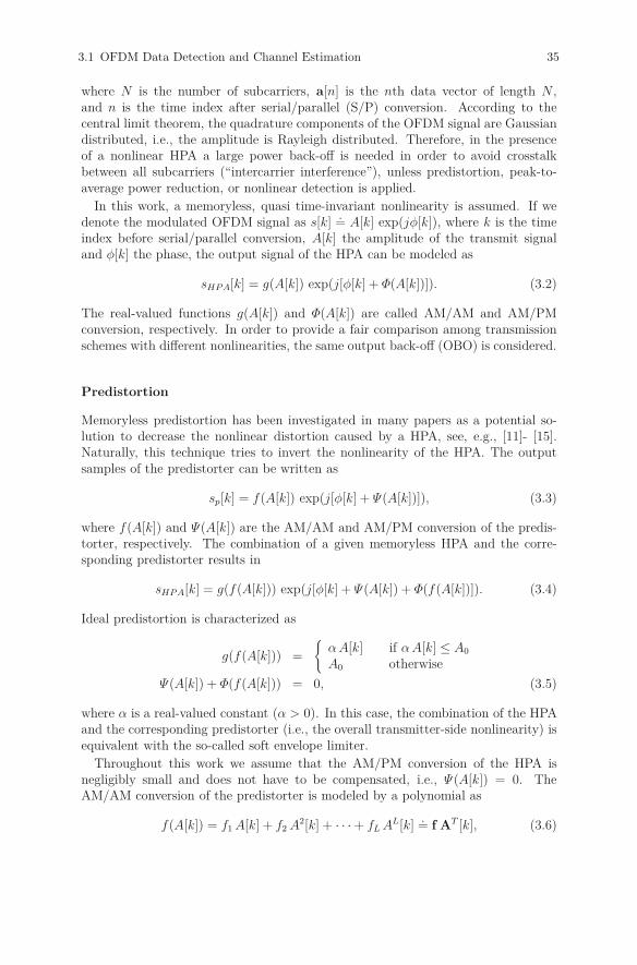
3.1 OFDM Data Detection and Channel Estimation 35
where N is the number of subcarriers, a[n] is the nth data vector of length N ,and n is the time index after serial/parallel (S/P) conversion. According to thecentral limit theorem, the quadrature components of the OFDM signal are Gaussiandistributed, i.e., the amplitude is Rayleigh distributed. Therefore, in the presenceof a nonlinear HPA a large power back-off is needed in order to avoid crosstalkbetween all subcarriers (“intercarrier interference”), unless predistortion, peak-to-average power reduction, or nonlinear detection is applied.
In this work, a memoryless, quasi time-invariant nonlinearity is assumed. If wedenote the modulated OFDM signal as s[k]
.= A[k] exp(jφ[k]), where k is the time
index before serial/parallel conversion, A[k] the amplitude of the transmit signaland φ[k] the phase, the output signal of the HPA can be modeled as
sHP A[k] = g(A[k]) exp(j[φ[k] + Φ(A[k])]). (3.2)
The real-valued functions g(A[k]) and Φ(A[k]) are called AM/AM and AM/PMconversion, respectively. In order to provide a fair comparison among transmissionschemes with different nonlinearities, the same output back-off (OBO) is considered.
Predistortion
Memoryless predistortion has been investigated in many papers as a potential so-lution to decrease the nonlinear distortion caused by a HPA, see, e.g., [11]- [15].Naturally, this technique tries to invert the nonlinearity of the HPA. The outputsamples of the predistorter can be written as
sp[k] = f(A[k]) exp(j[φ[k] + Ψ(A[k])]), (3.3)
where f(A[k]) and Ψ(A[k]) are the AM/AM and AM/PM conversion of the predis-torter, respectively. The combination of a given memoryless HPA and the corre-sponding predistorter results in
sHP A[k] = g(f (A[k])) exp(j[φ[k] + Ψ (A[k]) + Φ(f (A[k])]). (3.4)
Ideal predistortion is characterized as
g(f (A[k])) =
{α A[k] if α A[k] ≤ A0
A0 otherwise
Ψ (A[k]) + Φ(f (A[k])) = 0, (3.5)
where α is a real-valued constant (α > 0). In this case, the combination of the HPAand the corresponding predistorter (i.e., the overall transmitter-side nonlinearity) isequivalent with the so-called soft envelope limiter.
Throughout this work we assume that the AM/PM conversion of the HPA isnegligibly small and does not have to be compensated, i.e., Ψ (A[k]) = 0. TheAM/AM conversion of the predistorter is modeled by a polynomial as
f(A[k]) = f1 A[k] + f2 A2[k] + · · · + fL AL[k].= f AT [k], (3.6)
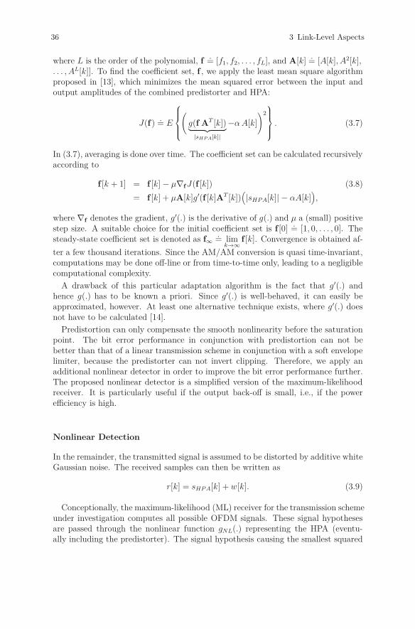
36 3 Link-Level Aspects
where L is the order of the polynomial, f.= [f1, f2, . . . , fL], and A[k]
.= [A[k], A2[k],
. . . , AL[k]]. To find the coefficient set, f , we apply the least mean square algorithmproposed in [13], which minimizes the mean squared error between the input andoutput amplitudes of the combined predistorter and HPA:
J(f).= E
⎧⎪⎪⎨⎪⎪⎩
(g(f AT [k])︸ ︷︷ ︸|sHP A[k]|
−α A[k]
)2
⎫⎪⎪⎬⎪⎪⎭ . (3.7)
In (3.7), averaging is done over time. The coefficient set can be calculated recursivelyaccording to
f [k + 1] = f [k] − μ∇f J(f [k]) (3.8)
= f [k] + μA[k]g′(f [k]AT [k])(|sHP A[k]| − αA[k]
),
where ∇f denotes the gradient, g′(.) is the derivative of g(.) and μ a (small) positivestep size. A suitable choice for the initial coefficient set is f [0]
.= [1, 0, . . . , 0]. The
steady-state coefficient set is denoted as f∞.= lim
k→∞f [k]. Convergence is obtained af-
ter a few thousand iterations. Since the AM/AM conversion is quasi time-invariant,computations may be done off-line or from time-to-time only, leading to a negligiblecomputational complexity.
A drawback of this particular adaptation algorithm is the fact that g′(.) andhence g(.) has to be known a priori. Since g′(.) is well-behaved, it can easily beapproximated, however. At least one alternative technique exists, where g′(.) doesnot have to be calculated [14].
Predistortion can only compensate the smooth nonlinearity before the saturationpoint. The bit error performance in conjunction with predistortion can not bebetter than that of a linear transmission scheme in conjunction with a soft envelopelimiter, because the predistorter can not invert clipping. Therefore, we apply anadditional nonlinear detector in order to improve the bit error performance further.The proposed nonlinear detector is a simplified version of the maximum-likelihoodreceiver. It is particularly useful if the output back-off is small, i.e., if the powerefficiency is high.
Nonlinear Detection
In the remainder, the transmitted signal is assumed to be distorted by additive whiteGaussian noise. The received samples can then be written as
r[k] = sHP A[k] + w[k]. (3.9)
Conceptionally, the maximum-likelihood (ML) receiver for the transmission schemeunder investigation computes all possible OFDM signals. These signal hypothesesare passed through the nonlinear function gNL(.) representing the HPA (eventu-ally including the predistorter). The signal hypothesis causing the smallest squared
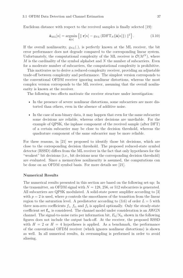
3.1 OFDM Data Detection and Channel Estimation 37
Euclidean distance with respect to the received samples is finally selected [19]:
aML[n] = argmina[n]
{‖ r[n] − gNL (IDFTN{a[n]}) ‖2
}. (3.10)
If the overall nonlinearity, gNL(.), is perfectly known at the ML receiver, the biterror performance does not degrade compared to the corresponding linear system.Unfortunately, the computational complexity of the ML receiver is O(MN ), whereM is the cardinality of the symbol alphabet and N the number of subcarriers. Evenfor a moderate number of subcarriers, the computational complexity is prohibitive.
This motivates us to derive a reduced-complexity receiver, providing an adjustabletrade-off between complexity and performance. The simplest version corresponds tothe conventional OFDM receiver ignoring nonlinear distortions, whereas the mostcomplex version corresponds to the ML receiver, assuming that the overall nonlin-earity is known at the receiver.
The following two effects motivate the receiver structure under investigation:
• In the presence of severe nonlinear distortions, some subcarriers are more dis-torted than others, even in the absence of additive noise.
• In the case of non-binary data, it may happen that even for the same subcarriersome decisions are reliable, whereas other decisions are unreliable. For theexample of QPSK, the inphase component of the received sample (after DFT)of a certain subcarrier may be close to the decision threshold, whereas thequadrature component of the same subcarrier may be more reliable.
For these reasons, in [21] we proposed to identify those bit decisions, which areclose to the corresponding decision threshold. The proposed reduced-state symboldetector (RSSD) differs from the ML receiver in the fact that only hypotheses for the“weakest” bit decisions (i.e., bit decisions near the corresponding decision threshold)are evaluated. Since a memoryless nonlinearity is assumed, the computations canbe done on an OFDM symbol basis. For more details see [21].
Numerical Results
The numerical results presented in this section are based on the following set-up: Inthe transmitter, an OFDM signal with N = 128, 256, or 512 subcarriers is generated.All subcarriers are QPSK modulated. A solid-state power amplifier according to [3]with p = 2 is used, where p controls the smoothness of the transition from the linearregion to the saturation level. A predistorter according to (3.6) of order L = 5 withthree non-zero coefficients f1, f3, and f5 is applied optionally. Only the steady-statecoefficient set f∞ is considered. The channel model under consideration is an AWGNchannel. The signal-to-noise ratio per information bit, Eb/N0, shown in the followingfigures does not include the output back-off. At the receiver, the proposed RSSDwith H = 2 or H = 4 hypotheses is applied. As a benchmark, the performanceof the conventional OFDM receiver (which ignores nonlinear distortions) is shownas well. In all numerical results, 4x oversampling is performed in order to avoidaliasing.
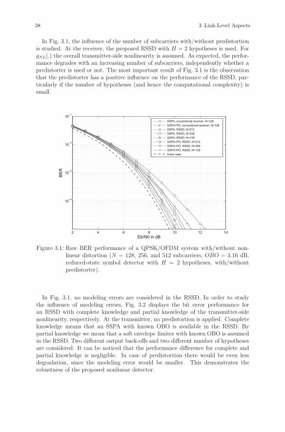
38 3 Link-Level Aspects
In Fig. 3.1, the influence of the number of subcarriers with/without predistortionis studied. At the receiver, the proposed RSSD with H = 2 hypotheses is used. ForgNL(.) the overall transmitter-side nonlinearity is assumed. As expected, the perfor-mance degrades with an increasing number of subcarriers, independently whether apredistorter is used or not. The most important result of Fig. 3.1 is the observationthat the predistorter has a positive influence on the performance of the RSSD, par-ticularly if the number of hypotheses (and hence the computational complexity) issmall.
2 4 6 8 10 12 14
10−4
10−3
10−2
10−1
Eb/N0 in dB
BE
R
SSPA, conventional receiver, N=128SSPA+PD, conventional receiver, N=128SSPA, RSSD, N=512SSPA, RSSD, N=256SSPA, RSSD, N=128SSPA+PD, RSSD, N=512SSPA+PD, RSSD, N=256SSPA+PD, RSSD, N=128linear case
Figure 3.1: Raw BER performance of a QPSK/OFDM system with/without non-linear distortion (N = 128, 256, and 512 subcarriers, OBO = 3.16 dB,reduced-state symbol detector with H = 2 hypotheses, with/withoutpredistorter).
In Fig. 3.1, no modeling errors are considered in the RSSD. In order to studythe influence of modeling errors, Fig. 3.2 displays the bit error performance foran RSSD with complete knowledge and partial knowledge of the transmitter-sidenonlinearity, respectively. At the transmitter, no predistortion is applied. Completeknowledge means that an SSPA with known OBO is available in the RSSD. Bypartial knowledge we mean that a soft envelope limiter with known OBO is assumedin the RSSD. Two different output back-offs and two different number of hypothesesare considered. It can be noticed that the performance difference for complete andpartial knowledge is negligible. In case of predistortion there would be even lessdegradation, since the modeling error would be smaller. This demonstrates therobustness of the proposed nonlinear detector.

3.1 OFDM Data Detection and Channel Estimation 39
2 4 6 8 10 12 14
10−4
10−3
10−2
10−1
Eb/N0 in dB
BE
R
RSSD (H=2) assuming HL, OBO=2.67dBRSSD (H=2) assuming SSPA, OBO=2.67dBRSSD (H=2) assuming HL, OBO=3.16dBRSSD (H=2) assuming SSPA, OBO=3.16dBRSSD (H=4) assuming HL, OBO=3.16dBRSSD (H=4) assuming SSPA, OBO=3.16dBlinear case
Figure 3.2: Raw BER performance of a QPSK/OFDM system with/without non-linear distortion (N = 128 subcarriers, OBO = 2.67 dB and 3.16 dB,no predistorter, reduced-state symbol detector with H = 2 and H = 4hypotheses, complete and partial knowledge of SSPA).
3.1.3 Joint Data Detection and Channel Estimation
In most OFDM systems, coherent data detection is applied, which a few exceptionslike Digital Audio Broadcasting (DAB). In order to support coherent detection,training symbols (pilot symbols) known at the receiver side are commonly used.In wireless OFDM systems, the training symbols may be either multiplexed withinthe data symbols in time and frequency domain, as firstly proposed in [22], orsuperimposed onto the data symbols, as suggested in [23]. For space limitations, werestrict ourself to the first case, since this technique became common in most state-of-the-art wireless OFDM systems. The main idea is to distribute the training symbolsin time and frequency domain. Assuming that the fading process is bandlimitedin time domain (since the Doppler power spectral density is typically bandlimited)and time-limited in frequency domain (since the delay power profile of a multipathchannel is typically time-limited). Given initial estimates at the positions of thetraining symbols, the channel coefficients (channel gains) can be reconstructed atthe data positions by means of interpolation or filtering [24]. A significant numberof papers on related techniques have been published.
The main drawback of training-based channel estimation is the overhead: anyadditional training symbol has an impact on power efficiency and bandwidth ef-ficiency. If channel coding is not taken into account for channel estimation, theminimum number of training symbols is dictated by the sampling theorem [22, 24].The training overhead is often acceptable in SISO systems, but in MIMO systemsthe required training overhead grows proportionally with the number of transmit
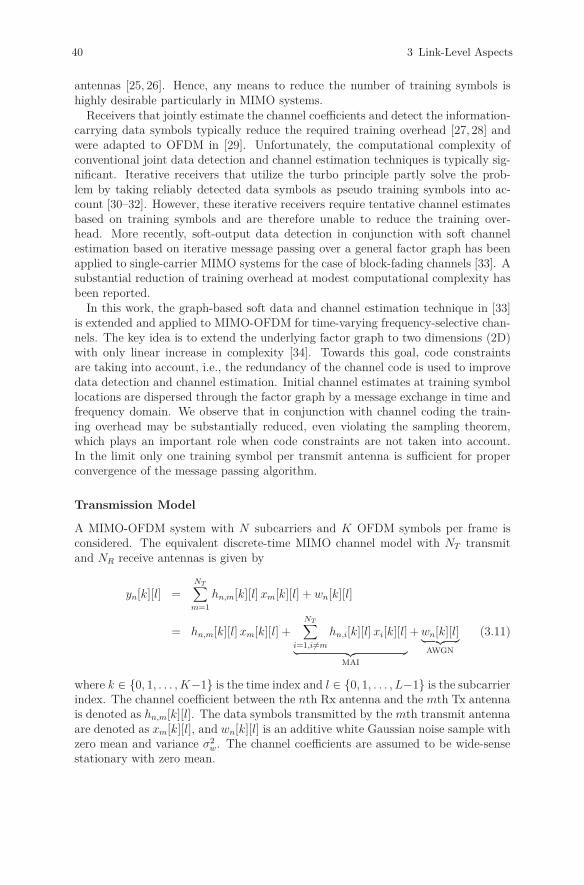
40 3 Link-Level Aspects
antennas [25, 26]. Hence, any means to reduce the number of training symbols ishighly desirable particularly in MIMO systems.
Receivers that jointly estimate the channel coefficients and detect the information-carrying data symbols typically reduce the required training overhead [27, 28] andwere adapted to OFDM in [29]. Unfortunately, the computational complexity ofconventional joint data detection and channel estimation techniques is typically sig-nificant. Iterative receivers that utilize the turbo principle partly solve the prob-lem by taking reliably detected data symbols as pseudo training symbols into ac-count [30–32]. However, these iterative receivers require tentative channel estimatesbased on training symbols and are therefore unable to reduce the training over-head. More recently, soft-output data detection in conjunction with soft channelestimation based on iterative message passing over a general factor graph has beenapplied to single-carrier MIMO systems for the case of block-fading channels [33]. Asubstantial reduction of training overhead at modest computational complexity hasbeen reported.
In this work, the graph-based soft data and channel estimation technique in [33]is extended and applied to MIMO-OFDM for time-varying frequency-selective chan-nels. The key idea is to extend the underlying factor graph to two dimensions (2D)with only linear increase in complexity [34]. Towards this goal, code constraintsare taking into account, i.e., the redundancy of the channel code is used to improvedata detection and channel estimation. Initial channel estimates at training symbollocations are dispersed through the factor graph by a message exchange in time andfrequency domain. We observe that in conjunction with channel coding the train-ing overhead may be substantially reduced, even violating the sampling theorem,which plays an important role when code constraints are not taken into account.In the limit only one training symbol per transmit antenna is sufficient for properconvergence of the message passing algorithm.
Transmission Model
A MIMO-OFDM system with N subcarriers and K OFDM symbols per frame isconsidered. The equivalent discrete-time MIMO channel model with NT transmitand NR receive antennas is given by
yn[k][l] =NT∑
m=1
hn,m[k][l] xm[k][l] + wn[k][l]
= hn,m[k][l] xm[k][l] +NT∑
i=1,i�=m
hn,i[k][l] xi[k][l]
︸ ︷︷ ︸MAI
+ wn[k][l]︸ ︷︷ ︸AWGN
(3.11)
where k ∈ {0, 1, . . . , K−1} is the time index and l ∈ {0, 1, . . . , L−1} is the subcarrierindex. The channel coefficient between the nth Rx antenna and the mth Tx antennais denoted as hn,m[k][l]. The data symbols transmitted by the mth transmit antennaare denoted as xm[k][l], and wn[k][l] is an additive white Gaussian noise sample withzero mean and variance σ2
w. The channel coefficients are assumed to be wide-sensestationary with zero mean.
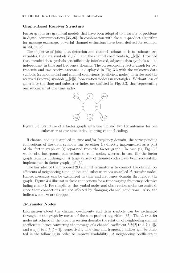
3.1 OFDM Data Detection and Channel Estimation 41
Graph-Based Receiver Structure
Factor graphs are graphical models that have been adopted to a variety of problemsin digital communications [35, 36]. In combination with the sum-product algorithmfor message exchange, powerful channel estimators have been derived for examplein [33, 37, 38].
The objective of joint data detection and channel estimation is to estimate twovariables, the data symbols xm[k][l] and the channel coefficients hn,m[k][l]. Providedthat encoded data symbols are sufficiently interleaved, adjacent data symbols will beindependent in time and frequency domain. The corresponding factor graph for twotransmit and two receive antennas is displayed in Fig. 3.3 with the unknown datasymbols (symbol nodes) and channel coefficients (coefficient nodes) in circles and thereceived (known) symbols yn[k][l] (observation nodes) in rectangles. Without loss ofgenerality the time and subcarrier index are omitted in Fig. 3.3, thus representingone subcarrier at one time index.
y1 y2
x2
h11
h21
h12x1
h22
Figure 3.3: Structure of a factor graph with two Tx and two Rx antennas for onesubcarrier at one time index ignoring channel coding.
If channel coding is applied in time and/or frequency domain, the correspondingconnections of the data symbols can be either (i) directly implemented as a partof the factor graph or (i) separated from the factor graph. In case (i), Fig. 3.3would also incorporate connections to code nodes, whereas in case (ii) the factorgraph remains unchanged. A large variety of channel codes have been successfullyimplemented in factor graphs, cf. [39].
The key idea of the proposed 2D channel estimator is to connect the channel co-efficients of neighboring time indices and subcarriers via so-called Δ-transfer nodes.Hence, messages can be exchanged in time and frequency domain throughout thegraph. Figure 3.4 illustrates these connections for a time-varying frequency-selectivefading channel. For simplicity, the symbol nodes and observation nodes are omitted,since their connections are not affected by changing channel conditions. Also, theindices n and m are dropped.
Δ-Transfer Nodes
Information about the channel coefficients and data symbols can be exchangedthroughout the graph by means of the sum-product algorithm [35]. The Δ-transfernodes introduced in the previous section describe the relation of neighboring channelcoefficients, hence converting the message of a channel coefficient h[k][l] to h[k +1][l]and h[k][l] to h[k][l + 1], respectively. The time and frequency indices will be omit-ted in the following in order to improve readability. A neighboring coefficient in
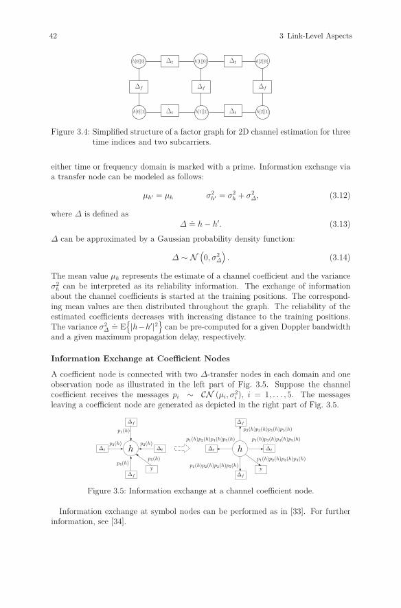
42 3 Link-Level Aspects
Δt
Δf Δf
Δt
Δf
h[0][0] h[1][0] h[2][0]
h[0][1] h[1][1] h[2][1]Δt Δt
Figure 3.4: Simplified structure of a factor graph for 2D channel estimation for threetime indices and two subcarriers.
either time or frequency domain is marked with a prime. Information exchange viaa transfer node can be modeled as follows:
μh′ = μh σ2h′ = σ2
h + σ2Δ, (3.12)
where Δ is defined asΔ
.= h − h′. (3.13)
Δ can be approximated by a Gaussian probability density function:
Δ ∼ N(0, σ2
Δ
). (3.14)
The mean value μh represents the estimate of a channel coefficient and the varianceσ2
h can be interpreted as its reliability information. The exchange of informationabout the channel coefficients is started at the training positions. The correspond-ing mean values are then distributed throughout the graph. The reliability of theestimated coefficients decreases with increasing distance to the training positions.The variance σ2
Δ.= E
{|h−h′|2
}can be pre-computed for a given Doppler bandwidth
and a given maximum propagation delay, respectively.
Information Exchange at Coefficient Nodes
A coefficient node is connected with two Δ-transfer nodes in each domain and oneobservation node as illustrated in the left part of Fig. 3.5. Suppose the channelcoefficient receives the messages pi ∼ CN (μi, σ2
i ), i = 1, . . . , 5. The messagesleaving a coefficient node are generated as depicted in the right part of Fig. 3.5.
Figure 3.5: Information exchange at a channel coefficient node.
Information exchange at symbol nodes can be performed as in [33]. For furtherinformation, see [34].
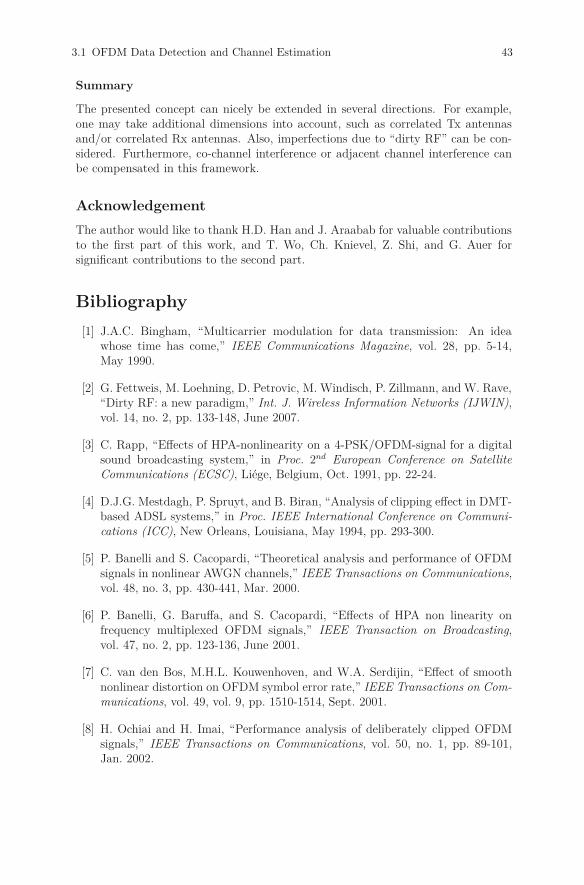
3.1 OFDM Data Detection and Channel Estimation 43
Summary
The presented concept can nicely be extended in several directions. For example,one may take additional dimensions into account, such as correlated Tx antennasand/or correlated Rx antennas. Also, imperfections due to “dirty RF” can be con-sidered. Furthermore, co-channel interference or adjacent channel interference canbe compensated in this framework.
Acknowledgement
The author would like to thank H.D. Han and J. Araabab for valuable contributionsto the first part of this work, and T. Wo, Ch. Knievel, Z. Shi, and G. Auer forsignificant contributions to the second part.
Bibliography
[1] J.A.C. Bingham, “Multicarrier modulation for data transmission: An ideawhose time has come,” IEEE Communications Magazine, vol. 28, pp. 5-14,May 1990.
[2] G. Fettweis, M. Loehning, D. Petrovic, M. Windisch, P. Zillmann, and W. Rave,“Dirty RF: a new paradigm,” Int. J. Wireless Information Networks (IJWIN),vol. 14, no. 2, pp. 133-148, June 2007.
[3] C. Rapp, “Effects of HPA-nonlinearity on a 4-PSK/OFDM-signal for a digitalsound broadcasting system,” in Proc. 2nd European Conference on SatelliteCommunications (ECSC), Liége, Belgium, Oct. 1991, pp. 22-24.
[4] D.J.G. Mestdagh, P. Spruyt, and B. Biran, “Analysis of clipping effect in DMT-based ADSL systems,” in Proc. IEEE International Conference on Communi-cations (ICC), New Orleans, Louisiana, May 1994, pp. 293-300.
[5] P. Banelli and S. Cacopardi, “Theoretical analysis and performance of OFDMsignals in nonlinear AWGN channels,” IEEE Transactions on Communications,vol. 48, no. 3, pp. 430-441, Mar. 2000.
[6] P. Banelli, G. Baruffa, and S. Cacopardi, “Effects of HPA non linearity onfrequency multiplexed OFDM signals,” IEEE Transaction on Broadcasting,vol. 47, no. 2, pp. 123-136, June 2001.
[7] C. van den Bos, M.H.L. Kouwenhoven, and W.A. Serdijin, “Effect of smoothnonlinear distortion on OFDM symbol error rate,” IEEE Transactions on Com-munications, vol. 49, vol. 9, pp. 1510-1514, Sept. 2001.
[8] H. Ochiai and H. Imai, “Performance analysis of deliberately clipped OFDMsignals,” IEEE Transactions on Communications, vol. 50, no. 1, pp. 89-101,Jan. 2002.

44 3 Link-Level Aspects
[9] E. Costa and S. Pupolin, “M-QAM-OFDM system performance in the presenceof a nonlinear amplifier and phase noise,” IEEE Transactions on Communica-tions, vol. 50, no. 3, pp. 462-472, Mar. 2002.
[10] K.R. Panta and J. Armstrong, “Effects of clipping on the error performance ofOFDM in frequency selective fading channels,” IEEE Transactions on WirelessCommunications, vol. 3, no. 2, pp. 668-671, Mar. 2004.
[11] G. Karam and H. Sari, “Analysis of predistortion, equalization, and ISI can-cellation techniques in digital radio systems with nonlinear transmit ampli-fiers,” IEEE Transactions on Communications, vol. 37, no. 12, pp. 1245-1253,Dec. 1989.
[12] K. Wesolowski and J. Pochmara, “Efficient algorithm for adjustment of adap-tive predistorter in OFDM transmitter,” in Proc. IEEE Vehicular TechnologyConference (VTC), Boston, Massachusetts, Sept. 2000, pp. 2491-2496.
[13] H. Besbes and T. Le-Ngoc, “A fast adaptive predistorter for nonlinearly am-plified M-QAM signals,” in Proc. IEEE Global Communications Conference(GLOBECOM), San Francisco, California, Nov.-Dec. 2000, pp. 108-112.
[14] Y. Guo and J.R. Cavallaro, “A novel adaptive pre-distorter using LS estimationof SSPA non-linearity in mobile OFDM systems,” in Proc. IEEE InternationalSymposium on Circuits and Systems (ISCAS), Phoenix, Arizona, May 2002,pp. 453-456.
[15] A. Behravan and T. Eriksson, “Baseband compensation techniques for band-pass nonlinearities,” in Proc. IEEE Vehicular Technology Conference, Orlando,Florida, Oct. 2003, pp. 279-283.
[16] S.H. Han and J.H. Lee, “An overview of peak-to-average power ratio reduc-tion techniques for multicarrier transmission,” IEEE Wireless Communications,vol. 12, no. 2, pp. 56-65, Apr. 2005.
[17] D. Declercq and G.B. Giannakis, “Recovering clipped OFDM symbols withBayesian inference,” in Proc. IEEE Int. Conference on Acoustics, Speech andSignal Processing (ICASSP), Istanbul, Turkey, June 2000, pp. 157-160.
[18] L. Junqiang, M. Zhengxin, and C. Zhigang, “Compensation of nonlinear distor-tion using a new method combining predistortion with reconstruction in OFDMsystems,” in Proc. Int. Conference on Communication Technology (ICCT), Bei-jing, China, Aug. 2000, pp. 769-772.
[19] J. Tellado, L.M.C Hoo, and J.M. Cioffi, “Maximum-likelihood detection of non-linearly distorted multicarrier symbols by iterative decoding,” IEEE Transac-tions on Communications, vol. 51, no. 2, pp. 218-228, Feb. 2003.
[20] P. Zillmann, “Soft detection and decoding of clipped and filtered COFDMsignals,” in Proc. IEEE Vehicular Technology Conference (VTC ’07-Spring),Dublin, Ireland, Apr. 2007.
Bibliography 45
[21] H.D. Han and P.A. Hoeher, “Predistortion and nonlinear detection for OFDMsignals in the presence of nonlinear high power amplification,” European Trans-actions on Telecommunications (ETT), vol. 18, pp. 411-418, June 2007.
[22] P. Hoeher, “TCM on frequency-selective land-mobile fading channels,” in Proc.5th Tirrenia Intern. Workshop on Digital Commun., Tirrenia, Italy, Sept. 1991,pp. 317-328.
[23] F. Tufvesson, M. Faulkner, P. Hoeher, and O. Edfors, “OFDM time and fre-quency synchronization by spread spectrum pilot technique,” in Proc. IEEEInternational Conference on Communications (ICC), Vancouver, Canada, June1999, pp. 115-119.
[24] P. Hoeher, S. Kaiser, and P. Robertson, “Two-dimensional pilot-symbol aidedchannel estimation by Wiener filtering,” in Proc. IEEE International Confer-ence on Acoustics, Speech, and Signal Processing (ICASSP), Munich, Germany,Apr. 1997, pp. 1845-1848.
[25] B. Hassibi and B.M. Hochwald, “How much training is needed in multiple-antenna wireless links?” IEEE Transactions on Information Theory, vol. 49,no. 4, pp. 951-963, Apr. 2003.
[26] I. Cosovic and G. Auer, “Capacity of MIMO-OFDM with pilot aided channelestimation,” EURASIP Journal on Wireless Communications and Networking,vol. 2007, no. 5, Jan. 2007.
[27] N. Seshadri, “Joint data and channel estimation using blind trellis search tech-niques,” IEEE Transactions on Communications, vol. 42, no. 2/3/4, pp. 1000-1011, Feb./Mar./Apr. 1994.
[28] E. Baccarelli and R. Cusani, “Combined channel estimation and data detec-tion using soft-statistics for frequency-selective fast-fading digital links,” IEEETransactions on Communications, vol. 46, no. 4, pp. 424-427, Apr. 1998.
[29] T. Cui and C. Tellambura, “Joint channel estimation and data detection forOFDM systems via sphere decoding,” in Proc. IEEE Global CommunicationsConference (GLOBECOM), Nov. 2004, pp. 3656-3660.
[30] M.C. Valenti and B.D. Woerner, “Iterative channel estimation and decoding ofpilot symbol assisted turbo codes over flat-fading channels,” IEEE Journal onSelected Areas in Communications, vol. 19, no. 9, pp. 1697-1705, Sept. 2001.
[31] F. Sanzi, S. Jelting, and J. Speidel, “A comparative study of iterative channelestimators for mobile OFDM systems,” IEEE Transaction on Wireless Com-munications, vol. 5, no. 2, pp. 849-859, Sept. 2003.
[32] G. Auer and J. Bonnet, “Threshold controlled iterative channel estimation forcoded OFDM,” in Proc. IEEE Vehicular Technology Conference (VTC-Spring),Dublin, Ireland, Apr. 2007, pp. 1737-1741.
46 3 Link-Level Aspects
[33] T. Wo, C. Liu, and P.A. Hoeher, “Graph-based soft channel and data estimationfor MIMO systems with asymmetric LDPC codes,” in Proc. IEEE InternationalConference on Communications (ICC), Beijing, China, May 2008, pp. 620-624.
[34] Ch. Knievel, Z. Shi, P.A. Hoeher, and G. Auer, “2D graph-based soft chan-nel estimation for MIMO-OFDM,” in Proc. IEEE International Conference onCommunications (ICC), Capetown, South Africa, May 2010.
[35] F.R. Kschischang, B.J. Frey, and H.-A. Loeliger, “Factor graphs and the sum-product algorithm,” IEEE Transactions on Information Theory, vol. 47, no. 2,pp. 498-519, Feb. 2001.
[36] H.A. Loeliger, J. Dauwels, J. Hu, S. Korl, L. Ping, and F.R. Kschischang, “Thefactor graph approach to model-based signal processing,” Proceedings of theIEEE, vol. 95, no. 6, pp. 1295-1322, June 2007.
[37] T. Wo, C. Liu, and P.A. Hoeher, “Graph-based iterative Gaussian detectionwith soft channel estimation for MIMO systems,” in Proc. ITG Conference onSource and Channel Coding (SCC), Ulm, Germany, Jan. 2008.
[38] T. Wo, J.Ch. Fricke, and P.A. Hoeher, “A graph-based iterative Gaussian detec-tor for frequency-selective MIMO channels,” in Proc. IEEE Information TheoryWorkshop (ITW), Chengdu, China, Oct. 2006, pp. 581-585.
[39] H.-A. Loeliger, “An introduction to factor graphs,” IEEE Signal ProcessingMagazine, vol. 21, no. 1, pp. 28-41, Jan. 2004.
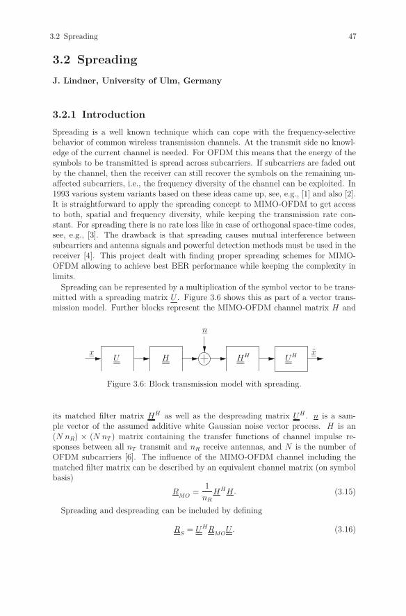
3.2 Spreading 47
3.2 Spreading
J. Lindner, University of Ulm, Germany
3.2.1 Introduction
Spreading is a well known technique which can cope with the frequency-selectivebehavior of common wireless transmission channels. At the transmit side no knowl-edge of the current channel is needed. For OFDM this means that the energy of thesymbols to be transmitted is spread across subcarriers. If subcarriers are faded outby the channel, then the receiver can still recover the symbols on the remaining un-affected subcarriers, i.e., the frequency diversity of the channel can be exploited. In1993 various system variants based on these ideas came up, see, e.g., [1] and also [2].It is straightforward to apply the spreading concept to MIMO-OFDM to get accessto both, spatial and frequency diversity, while keeping the transmission rate con-stant. For spreading there is no rate loss like in case of orthogonal space-time codes,see, e.g., [3]. The drawback is that spreading causes mutual interference betweensubcarriers and antenna signals and powerful detection methods must be used in thereceiver [4]. This project dealt with finding proper spreading schemes for MIMO-OFDM allowing to achieve best BER performance while keeping the complexity inlimits.
Spreading can be represented by a multiplication of the symbol vector to be trans-mitted with a spreading matrix U . Figure 3.6 shows this as part of a vector trans-mission model. Further blocks represent the MIMO-OFDM channel matrix H and
xHH UHH
x
n
U
Figure 3.6: Block transmission model with spreading.
its matched filter matrix HH as well as the despreading matrix UH . n is a sam-ple vector of the assumed additive white Gaussian noise vector process. H is an(N nR) × (N nT ) matrix containing the transfer functions of channel impulse re-sponses between all nT transmit and nR receive antennas, and N is the number ofOFDM subcarriers [6]. The influence of the MIMO-OFDM channel including thematched filter matrix can be described by an equivalent channel matrix (on symbolbasis)
RMO
=1
nR
HHH. (3.15)
Spreading and despreading can be included by defining
RS
= UHRMO
U. (3.16)
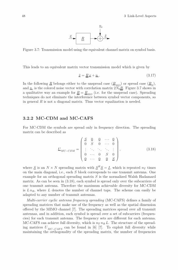
48 3 Link-Level Aspects
nc
xxR
Figure 3.7: Transmission model using the equivalent channel matrix on symbol basis.
This leads to an equivalent matrix vector transmission model which is given by
x = R x + nc. (3.17)
In the following R belongs either to the unspread case (RMO
) or spread case (RS),
and nc is the colored noise vector with correlation matrix 2N0R. Figure 3.7 shows ina qualitative way an example for R = R
MO(i.e. for the unspread case). Spreading
techniques do not eliminate the interference between symbol vector components, soin general R is not a diagonal matrix. Thus vector equalization is needed.
3.2.2 MC-CDM and MC-CAFS
For MC-CDM the symbols are spread only in frequency direction. The spreadingmatrix can be described as
UMC−CDM
=
⎛⎜⎜⎜⎜⎜⎜⎜⎝
S 0 0 · · · 00 S 0 · · · 0...
. . . . . . . . ....
0 · · · 0 S 00 · · · 0 0 S
⎞⎟⎟⎟⎟⎟⎟⎟⎠
, (3.18)
where S is an N × N spreading matrix with SHS = I, which is repeated nT timeson the main diagonal, i.e., each S block corresponds to one transmit antenna. Oneexample for an orthogonal spreading matrix S is the normalized Walsh Hadamardmatrix. As can be seen in (3.18), each symbol is spread only over the subcarriers ofone transmit antenna. Therefore the maximum achievable diversity for MC-CDMis L nR, where L denotes the number of channel taps. The scheme can easily beadapted to any number of transmit antennas.
Multi-carrier cyclic antenna frequency spreading (MC-CAFS) defines a family ofspreading matrices that make use of the frequency as well as the spatial dimensionoffered by the MIMO channel [7]. The spreading matrices spread over all transmitantennas, and in addition, each symbol is spread over a set of subcarriers (frequen-cies) for each transmit antenna. The frequency sets are different for each antenna.MC-CAFS can achieve full diversity, which is nT nR L. The structure of the spread-ing matrices U
MC−CAF Scan be found in [6] [7]. To exploit full diversity while
maintaining the orthogonality of the spreading matrix, the number of frequencies

3.2 Spreading 49
subchannel #
subc
hann
el #
5 10 15 20 25 30
5
10
15
20
25
30
a)
5 10 15 20 25 300
0.2
0.4
0.6
0.8
1
1.2
1.4
1.6
subchannel #
|dia
g(R
)|
b)
Figure 3.8: Equivalent channel matrix for unspread MIMO-OFDM. a) RMO
for nT =nR = 4, N = 8 subcarriers, and L = 4 paths. (b) Absolute value of thediagonal elements of R
MO.
B, over which each symbol is spread, should fulfill the following conditions:
L ≤ B ≤ N/nT . (3.19)
Figures 3.8 to 3.10 demonstrate the effect of spreading on the equivalent channelmatrix R for a frequency-selective time-invariant channel with L = 4 taps. Figure3.8 is for the unspread case. Although the probability of a deep fade is reduced bythe multiple receive antennas and maximum ratio combining, the elements on themain diagonal have a large variance. With MC-CDM spreading (see Fig. 3.9) wecan observe that the diagonal elements have the same value within each transmitantenna block, but vary from block to block. This is due to the fact that the symbolenergy is spread over all frequencies of each antenna separately, but no spreading inantenna direction is applied. The new scheme, i.e., MC-CAFS, includes spreading infrequency and space direction. If the parameters of the spreading matrix are chosenproperly, it is possible to achieve constant diagonal elements on the main diagonalof R as can be seen in Fig. 3.10. This means, the matched filter bound (MFB)coincides with the AWGN performance.
3.2.3 Simulation Results
Figures 3.11 and 3.12 show a comparison of different spreading schemes for uncodedand coded transmissions, respectively. The channel was a block fading channelstaying constant during one OFDM symbol block, but changes independently fromblock to block. For equalization, a soft Cholesky equalizer (SCE) [8] was used. Theresults for uncoded transmission in Fig. 3.11 show that exploiting additional diversityby spreading improves the performance substantially compared to unspread OFDM.MC-CAFS outperforms MC-CDM both for a channel length of L = 2 and L = 4due to the additional transmit antenna diversity. Figure 3.12 shows the resultsfor coded transmissions using a convolutional code with memory 2 and iterativeequalization and decoding. The results for code rate 3/4 in Fig. 3.12 b) were obtained

50 3 Link-Level Aspects
subchannel #
subc
hann
el #
5 10 15 20 25 30
5
10
15
20
25
30
a)
subchannel #
subc
hann
el #
5 10 15 20 25 30
5
10
15
20
25
30
b)
5 10 15 20 25 300
0.1
0.2
0.3
0.4
0.5
0.6
0.7
0.8
0.9
1
subchannel #
|dia
g(R
)|
c)
Figure 3.9: Equivalent channel matrix for MC-CDM: a) spreading matrixU
MC−CDM; b) R
MC−CDMfor nT = nR = 4, N = 8 subcarriers, and
L = 4 paths; c) absolute value of the diagonal elements of RMC−CDM
.
subchannel #
subc
hann
el #
5 10 15 20 25 30
5
10
15
20
25
30
a)
subchannel #
subc
hann
el #
5 10 15 20 25 30
5
10
15
20
25
30
b)
5 10 15 20 25 300
0.1
0.2
0.3
0.4
0.5
0.6
0.7
0.8
0.9
1
subchannel #
|dia
g(R
)|
c)
Figure 3.10: Equivalent channel matrix for MC-CAFS: a) spreading matrixU
MC−CAF S; b) R
MC−CAF Sfor nT = nR = 4, N = 8 subcarriers, and
L = 4 paths; c) absolute value of the diagonal elements of RMC−CAF S
.
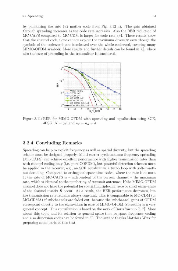
3.2 Spreading 51
by puncturing the rate 1/2 mother code from Fig. 3.12 a). The gain obtainedthrough spreading increases as the code rate increases. Also the BER reduction ofMC-CAFS compared to MC-CDM is larger for code rate 3/4. These results showthat the channel code alone cannot exploit the maximum diversity even though thesymbols of the codewords are interleaved over the whole codeword, covering manyMIMO-OFDM symbols. More results and further details can be found in [6], wherealso the case of precoding in the transmitter is considered.
Figure 3.11: BER for MIMO-OFDM with spreading and equalization using SCE,4PSK, N = 32, and nT = nR = 4.
3.2.4 Concluding Remarks
Spreading can help to exploit frequency as well as spatial diversity, but the spreadingscheme must be designed properly. Multi-carrier cyclic antenna frequency spreading(MC-CAFS) can achieve excellent performance with higher transmission rates thanwith channel coding only (i.e. pure COFDM), but powerful detection schemes mustbe applied in the receiver, e.g., an SCE equalizer in a turbo loop with soft-in-soft-out decoding. Compared to orthogonal space-time codes, where the rate is at most1, the rate of MC-CAFS is – independent of the current channel – the maximumrate, which is identical to the number nT of transmit antennas. If the MIMO-OFDMchannel does not have the potential for spatial multiplexing, zero or small eigenvaluesof the channel matrix R occur. As a result, the BER performance decreases, butthe transmission rate remains always constant. This is comparable to MC-CDM (orMC-CDMA) if subchannels are faded out, because the subchannel gains of OFDMcorrespond directly to the eigenvalues in case of MIMO-OFDM. Spreading is a verygeneral concept. This contribution is based on the work of Doris Yacoub [5–7]. Moreabout this topic and its relation to general space-time or space-frequency codingand also dispersion codes can be found in [9]. The author thanks Matthias Wetz forpreparing some parts of this text.

52 3 Link-Level Aspects
E /N [dB]b 0
a) code rate 1/2
E /N [dB]b 0
b) code rate 3/4
Figure 3.12: BER of MIMO-OFDM 4PSK with convolutional code, memory 2, nT =nR = 4, N = 32, and L = 4.
Bibliography
[1] K. Fazel. “Performance of CDMA/OFDM for Mobile Communication Systems,”Proc. ICUPC ’93, pp. 975-979, 1993.
[2] J. Lindner, “MC-CDMA in the context of general multiuser/multisubchanneltransmission methods,” ETT, European Transactions on Telecommunications,vol. 10, no. 4, pp. 351-367, 1999.
[3] V. Tarokh, H. Jafarkhani, and A.R. Calderbank, “Space-time block codes fromorthogonal designs,” IEEE Trans. Inform. Theory, vol. 45, no 5, 1999.
[4] D. Y. Yacoub, W. G. Teich, and J. Lindner, “Effect of Antenna Correlations onInterference and Performance of a Spread MIMO-OFDM System (MC-CAFS),”11th International OFDM-Workshop 2006, Hamburg / Germany, Aug. 2006.
[5] D. Y. Yacoub, W. G. Teich, and J. Lindner, “Precoding and Spreading forMIMO-OFDM in the Presence of Antenna Correlations,” 12th InternationalOFDM-Workshop 2007, Hamburg / Germany, Aug. 2007.
[6] D. Y. Yacoub, Spreading and Coding for Wireless MIMO-OFDM Systems, Dis-sertation, Institute for Information Technology, University of Ulm, June 2008.
[7] D. Y. Yacoub, W. G. Teich, and J. Lindner, “MC-Cyclic Antenna FrequencySpread: A Novel Space-Frequency Spreading for MIMO-OFDM,” 8th Inter-national Symposium on Communication Theory and Applications (ISCTA ’05),Ambleside, Lake District / UK, July 2005.
[8] J. Egle, C. Sgraja, and J. Lindner, “Iterative soft Cholesky block decision feed-back equalizer - a promising approach to combat interference,” in Proc. IEEE

Bibliography 53
Vehicular Technology Conference (VTC Spring), vol. 3, Rhodes / Greece, May2001, pp. 1604-1608.
[9] C. Pietsch, Coherent Space Time Block Codes from Sets of Subspaces, Disserta-tion, Institute for Information Technology, University of Ulm, October 2008.

54 3 Link-Level Aspects
3.3 Iterative Diversity Reception for Coded
OFDM Transmission Over Fading Channels
M. Matuszak, R. Urbansky, University of Kaiserslautern, Germany
3.3.1 Introduction
Time- and frequency-selective fading resulting from time-variant multipath propaga-tion can be mitigated by forward error correction (FEC) channel coding in combina-tion with time and frequency interleaving. In broadband systems coded orthogonalfrequency-division multiplexing (COFDM) is a well-known implementation of thisconcept, which is applied, e.g., in digital terrestrial video broadcasting (DVB-T),Digital Audio Broadcasting (DAB), and Digital Radio Mondiale (DRM) [1] [4].
A bandwidth of 1.5 MHz for DAB or 8 MHz for DVB-T enables efficient frequencyinterleaving to mitigate fading. However, DRM is restricted to a bandwidth of upto 20 kHz for compatibility to existing services [3]. In addition, DRM transmissionespecially in short-wave bands is characterized by time varying ionospheric fading.Whereas fast fading is covered by time interleaving, long-term frequency-selectivefading severely affects transmission, since a narrow bandwidth results in a highpercentage of subcarriers with low signal-to-noise ratio (SNR), which may exceedFEC capabilities.
Diversity techniques also allow to mitigate fading [5]. COFDM systems, e.g., caninherently utilize delay diversity or path diversity in single frequency networks, pro-vided the OFDM guard interval covers the maximum path or delay spread [1]. Inaddition, for narrow-band systems like DRM, antenna diversity, polarization diver-sity and especially frequency diversity may also be taken into account. Receiverconcepts for frequency or antenna diversity usually apply combining techniques, likeselection combining, equal gain combining or maximum ratio combining (MRC).In general, these methods combine the properly equalized and synchronized analogsignals before FEC decoding.
We proposed a different approach: since diversity transmission of FEC encodeddata can be regarded as a parallel concatenated coding scheme which allows forturbo decoding, we combine the received and appropriately equalized signals in aniterative decoding process, see Fig. 3.13 [3].
Propagating extrinsic information in terms of log-likelihood-ratio (LLR), the turbodiversity (TD) scheme delivers additional iteration gains compared to MRC [2].This requires that the constituent component codes, usually punctured convolutionalcodes (CC), have to be chosen appropriately by applying extrinsic information trans-fer (EXIT) chart methods. Instead of CC, codes can be also applied, where againthese methods have been used [7]. The project focuses mainly on LDPC codes asconstituent codes, because they are known to approach the Shannon limit as closeas Turbo codes (TC) [8] and efficient soft-input soft-output decoding algorithmsare available.

3.3 Iterative Diversity Reception for Coded OFDM Transmission 55
� � � �
� � � � � � �
� � � �
� � � � � � �
� �
� �
� �
� �
� �
� �
� �
� �
� �
� �
� � � � � � � � � � � � � � � � � � �
� �
� �
� �
� �
� �
� �
� �
� �
� � � � �
�
� � � � �
�
� �
� �
� � � �
� � � � � � �
� � � �
� � � � � � �
� � � �
� � � � � � � � �
� � � �
� � � � � � � � �
� � � �
� � � � � � � � �
� � � �
� � � � � � � � �
� � � � � � � � �
� � � � � � � � �
�
�
��
�
�
�
��
�
�
�
�
� � � � � � � � � � �
� � � � � � � � � � �
� � � � � � � � � � � � � � � � � � � � � � � � � � �
� �
� �
�
�
� � � � � �
� � � � � �
�
�
�
�
�
� � � � � � � � � � �
�
�
�
�
�
Figure 3.13: Iterative diversity receiver for OFDM systems.
3.3.2 Turbo Diversity
A soft-input soft-output (SISO) decoder which allows for propagating extrinsic in-formation is the key element of the turbo decoding principle [6]. Therefore, anoptimum maximum-a-posteriori symbol-by-symbol estimator like the Bahl-Cocke-Jelinek-Raviv (BCJR) algorithm for turbo codes or the sum-product algorithm [7]for LDPC codes have be applied, calculating for each bit ck the LLR conditioned onthe received sequence
Λ (ck|r) = ln (P (ck = 1|r) /P (ck = 0|r)) (3.20)
According to the turbo decoding principle, extrinsic information Λe is exchangedbetween the decoding stages, where for Λe any a-priori information has to be sub-tracted from the BCJR output reliability information, see Fig. 3.13.
The iteration process can be visualized by EXIT charts, where the mutual infor-mation (MI) of one decoder is plotted versus its a-priori input, i.e., the MI of theother decoder [9]. Using optimum decoders, the knowledge of the MI contained inits a-priori information is sufficient to derive the MI of Λe delivered by this decoder.
Figure 3.13 motivates the similarity of TC and TD. Consequently, EXIT chartmethods considering the constituent LDPC codes allow for analyzing the iterationprocess of TD. In this case EXIT functions are derived from the parameters of LDPCcodes, namely coefficients of degree distributions of variable nodes λ(x) and of check
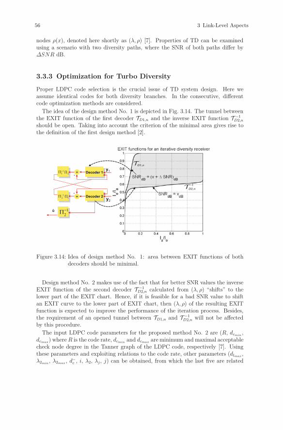
56 3 Link-Level Aspects
nodes ρ(x), denoted here shortly as (λ, ρ) [7]. Properties of TD can be examinedusing a scenario with two diversity paths, where the SNR of both paths differ byΔSNR dB.
3.3.3 Optimization for Turbo Diversity
Proper LDPC code selection is the crucial issue of TD system design. Here weassume identical codes for both diversity branches. In the consecutive, differentcode optimization methods are considered.
The idea of the design method No. 1 is depicted in Fig. 3.14. The tunnel betweenthe EXIT function of the first decoder TD1,n and the inverse EXIT function T −1
D2,n
should be open. Taking into account the criterion of the minimal area gives rise tothe definition of the first design method [2].
� � � � � � � � �
� � � � � � � � �
�
�
��
�
�
�
��
�
�
�
�
�
�
�
�
�
�
�
�� � � �
�� � � �
� �
� �
� �
Figure 3.14: Idea of design method No. 1: area between EXIT functions of bothdecoders should be minimal.
Design method No. 2 makes use of the fact that for better SNR values the inverseEXIT function of the second decoder T −1
D2,n calculated from (λ, ρ) “shifts” to thelower part of the EXIT chart. Hence, if it is feasible for a bad SNR value to shiftan EXIT curve to the lower part of EXIT chart, then (λ, ρ) of the resulting EXITfunction is expected to improve the performance of the iteration process. Besides,the requirement of an opened tunnel between TD1,n and T −1
D2,n will not be affectedby this procedure.
The input LDPC code parameters for the proposed method No. 2 are (R, dcmin,
dcmax) where R is the code rate, dcmin and dcmax are minimum and maximal acceptablecheck node degree in the Tanner graph of the LDPC code, respectively [7]. Usingthese parameters and exploiting relations to the code rate, other parameters (dlmax,λ2min , λ2max , d−c , i, λ2, λj, j) can be obtained, from which the last five are related
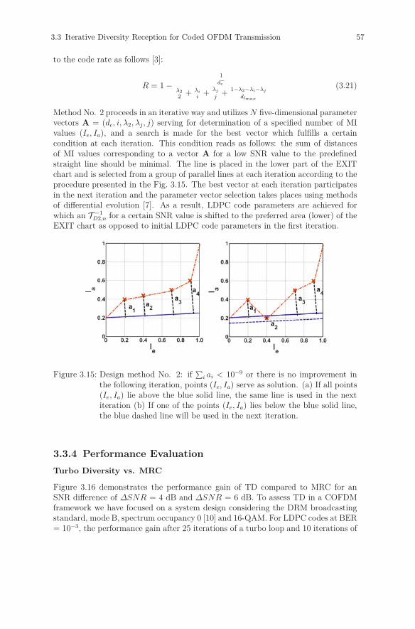
3.3 Iterative Diversity Reception for Coded OFDM Transmission 57
to the code rate as follows [3]:
R = 1 −1
d−c
λ2
2+ λi
i+ λj
j+ 1−λ2−λi−λj
dlmax
(3.21)
Method No. 2 proceeds in an iterative way and utilizes N five-dimensional parametervectors A = (dc, i, λ2, λj, j) serving for determination of a specified number of MIvalues (Ie, Ia), and a search is made for the best vector which fulfills a certaincondition at each iteration. This condition reads as follows: the sum of distancesof MI values corresponding to a vector A for a low SNR value to the predefinedstraight line should be minimal. The line is placed in the lower part of the EXITchart and is selected from a group of parallel lines at each iteration according to theprocedure presented in the Fig. 3.15. The best vector at each iteration participatesin the next iteration and the parameter vector selection takes places using methodsof differential evolution [7]. As a result, LDPC code parameters are achieved forwhich an T −1
D2,n for a certain SNR value is shifted to the preferred area (lower) of theEXIT chart as opposed to initial LDPC code parameters in the first iteration.
Figure 3.15: Design method No. 2: if∑
i ai < 10−9 or there is no improvement inthe following iteration, points (Ie, Ia) serve as solution. (a) If all points(Ie, Ia) lie above the blue solid line, the same line is used in the nextiteration (b) If one of the points (Ie, Ia) lies below the blue solid line,the blue dashed line will be used in the next iteration.
3.3.4 Performance Evaluation
Turbo Diversity vs. MRC
Figure 3.16 demonstrates the performance gain of TD compared to MRC for anSNR difference of ΔSNR = 4 dB and ΔSNR = 6 dB. To assess TD in a COFDMframework we have focused on a system design considering the DRM broadcastingstandard, mode B, spectrum occupancy 0 [10] and 16-QAM. For LDPC codes at BER= 10−3, the performance gain after 25 iterations of a turbo loop and 10 iterations of

58 3 Link-Level Aspects
the LDPC decoder compared to MRC with 250 LDPC decoding iterations is in theorder of 1.5 dB and 3 dB, for ΔSNR = 4 dB and ΔSNR = 6 dB, respectively. Inthe case of turbo codes, where only 10 iterations of a turbo loop and 10 iterationsof the inner decoder were considered in order to ensure a comparable computationaleffort, TD outperforms MRC by ca. 1.5 dB.
0 1 2 3 4 510−7
10−6
10−5
10−4
10−3
10−2
10−1
Eb/N0 / dB
BE
R
Turbo Diversity, ΔSNR = 4 dB, LDPC C.Turbo Diversity, ΔSNR = 4 dB, Turbo C.Turbo Diversity, ΔSNR = 6 dB, LDPC C.LLR−Combining, ΔSNR = 4 dB, LDPC C.LLR−Combining, ΔSNR = 4 dB, Turbo C.LLR−Combining, ΔSNR = 6 dB, LDPC C.
Figure 3.16: BER performance of MRC and TD using LDPC codes, turbo codes andRSCC (CC) for a DRM-based scenario.
LDPC Code Design
Wiener filterThe performance analysis was carried out for an OFDM scenario in which the
channel profile followed “US Consortium” with path delays (1, 0.7, 1.5, 2.2 ms),path gains (1, 0.7, 0.5, 0.25) and normalized Doppler frequency fD = 0.05. Channelestimation was implemented using the Wiener filter method [11] and LDPC codesof rate 3/4 and block length 9000 were used.
EXIT characteristics are depicted for both code design techniques in Fig. 3.17a), where the corresponding LDPC code parameters are (λ2= 0.198, λ4= 0.2441,λ5= 0.1421, λ29= 0.093, λ30= 0.151, λ34 = 0.1715, ρ19= 0.1655, ρ20= 0.8345) and(λ2= 0.441, λ30= 0.5589, ρ16= 0.2644, ρ17= 0.7356), respectively. The resultingEXIT functions of method No. 2, for low SNRs are wider opened than EXIT func-tions of method No. 1, what can be understood as better performance for a lowernumber of iterations. Despite of another design criterion for method No. 2, the areabetween resulting EXIT functions is smaller than for method No. 1, which is relatedto a lower distance to channel capacity.

3.3 Iterative Diversity Reception for Coded OFDM Transmission 59
0 0.2 0.4 0.6 0.8 10
0.1
0.2
0.3
0.4
0.5
0.6
0.7
0.8
0.9
1
Ia/Ie
I e/I a
EbN0 = 1.7 dB, altes OptimierungsverfahrenEbN0 = − 2.3 dB, altes OptiemierungsverfahrenEbN0 = 1.7 dB, neues OptimierungsverfahrenEbN0 = −2.3 dB, neues Optimierungsverfahren
(a)
6 6.5 7 7.5 8 8.5 9 9.510−7
10−6
10−5
10−4
10−3
10−2
10−1
Eb/N0 / dB
BE
R
ΔSNR = 4 dB, method No. 2
ΔSNR = 4 dB, method No. 1
ΔSNR = 6 dB, method No. 2
ΔSNR = 6 dB, method No. 1
(b)
Figure 3.17: Performance analysis of Turbo Diversity with optimized LDPC codesfor different code design methods a) EXIT functions, b) BER perfor-mance of TD with difference between diversity paths ΔSNR = 4 dBand ΔSNR = 6 dB
Comparing the performance of these methods for the first and the second scenario(Fig. 3.17 b) ), considering BER=10−3 it can be seen that for TD method No. 2outperforms method No. 1. For LDPC codes with blocks of 9000 bits this gap isnearly 0.9 dB. Superiority of method No. 2 does not depend on the fading scenariobut it should be mentioned that LDPC codes achieved by means of the method No.2 turn to be worse for the system without TD (only one path) and on AdditiveWhite Gaussian Noise channel.
3.3.5 Summary
In this contribution we investigated Turbo Diversity as an iterative decoding conceptfor diversity systems which outperforms MRC in single carrier and OFDM systems.Additional gains are achieved by using optimized LDPC codes as constituent codes.Two different criteria were proposed for the LDPC code design adapted to TD withOFDM. The method using the design goal to position the inverse EXIT function inthe preferred area outperforms the classical criterion aimed at minimal area betweenEXIT functions. Despite of the fact that the area between EXIT characteristics doesnot have first priority in our new method, this area turns out to be less than in thecase of the classical method, thus fulfilling both criteria in a better way and reducingthe distance to channel capacity. The new method is better suited for differentfading scenarios and block lengths of LDPC codes, what proves its robustness. Forpractical applications of TD the new method to design constituent LDPC codesdelivers a robust approach for different fading scenarios and block lengths of LDPCcodes.

60 3 Link-Level Aspects
Bibliography
[1] R. van Nee and R. Prassad, OFDM for Wireless Multimedia Communications,Artech House Publishers, Norwood, MA., USA, 2000.
[2] M. Matuszak, W. Sauer-Greff and R. Urbansky, “Iterative Diversity ReceiverConcept for Narrow-Band OFDM Systems,” in Proc. 13. International OFDMWorkshop, pp. 251-255, Hamburg, Germany, 2008.
[3] M. Matuszak, W. Sauer-Greff and R. Urbansky, “EXIT Chart Based LDPCCode Design for Iterative Diversity Receivers in OFDM Systems with FadingChannels,” in Proc. 14. International OFDM Workshop, pp. 20-24, Hamburg,Germany, 2009.
[4] A. Dittrich, T. Schorr and R. Urbansky, “Diorama - A MATLAB Based OpenSource Software Radio for Digital Radio Mondiale (DRM),” in Proc. 10. Inter-national OFDM-Workshop, pp. 391-395, Hamburg, Germany, 2005.
[5] A. Paulraj, “Diversity Techniques,” in J.D. Gibson (Ed.) The Mobile Commu-nication Handbook, pp. 166-176, CRC Press, Boca Raton, FL., USA, 1996.
[6] J. Hagenauer, “Das Turbo-Prinzip in Detektion und Decodierung,” in ITG-Fachberichte, Vol. 146, pp. 131-136, 1998.
[7] T. Richardson, M. Shokrollahi and R. Urbanke, “Design of Capacity-Approaching Irregular Low-Density Parity-Check Codes,” IEEE Trans. onInform. Theory, Vol. 47, No. 2, pp. 619-637, Febr. 2001.
[8] L. Bahl, J. Cocke, F. Jelinek and J. Raviv, “Optimal Decoding of Linear Codesfor Minimizing Symbol Error Rate,” IEEE Trans. on Inform. Theory, Vol. 20,No. 2, pp. 284-287, March 1974.
[9] S. ten Brink, “Convergence Behavior of Iteratively Decoded Parallel Con-catenated Codes,” IEEE Transactions on Communications, Vol. 49, No. 10,pp. 1727-1737, Oct. 2001.
[10] European Telecommunications Standard Institute (ETSI), Digital Radio Mon-diale (DRM); System Specification, ETSI ES 201 980 V2.1.1, Sophia AntipolisCedex, France, 2004.
[11] C. Sgraja and J. Linder, “Estimation of Rapid Time-Variant Channels forOFDM using Wiener Filtering,” in Proc. IEEE International Conference onCommunications (ICC), Vol. 4, pp. 2390-2395, AK., USA, May 2003.
3.4 MMSE-based Turbo Equalization Principles 61
3.4 MMSE-based Turbo Equalization Principles
for Frequency Selective Fading Channels
M. Grossmann, R. Thomä, Ilmenau University of Technology, Germany
3.4.1 Introduction
Turbo equalization [1–11] is one of the most promising techniques to implementpowerful equalizers, without requiring high computational complexity, for codedcommunication systems with frequency-selective fading channels. The complexityadvantage of turbo equalizers is due to the separation of channel equalization anddecoding into two basic processors, while the high performance is achieved by ex-changing soft information between these two components in an iterative manner.The turbo equalization approach was originally proposed in [1], utilizing a maximuma posteriori probability (MAP) algorithm for iterative equalization in frequency-selective fading channels. However, because of its exponentially increasing complex-ity, the MAP-based equalizer is only practical for simple modulation formats, likebinary phase shift keying (BPSK), and for channels with less multi-path components.In [2], the optimal MAP algorithm has been replaced by a low-cost alternative basedon the soft cancellation (SC) and minimum mean-squared error (MMSE) principle.The SC-MMSE filtering approach in [2], originally proposed for detection of randomcoded code-division multiple-access (CDMA) signals, has been applied to channelequalization in [3], and to multiple-input multiple-output (MIMO) channel equaliza-tion in [4]. Recently, the SC-MMSE turbo concept has also been used to equalizationof OFDM systems in time-varying channels [5].
In this contribution, we discuss three extensions of the basic SC-MMSE filter-ing concept for turbo equalization. In particular, we first propose a novel fre-quency domain (FD) turbo equalizer for MIMO-OFDM transmissions with insuf-ficient guard interval. The SC-MMSE-based equalizer exploits the banded structureof the FD channel matrices, allowing the implementation of the equalizer with acomplexity which is only linear in the number of sub-carriers. We then present ahybrid turbo equalizer, suitable for multi-user OFDM transmissions with spatially-correlated channels, that combines SC-MMSE filtering and MAP-detection. Finally,we propose a nonlinear MMSE-based turbo equalizer for single-carrier spatially-multiplexed MIMO transmissions with high-rate codes.
3.4.2 System Model
Consider the discrete-time baseband equivalent model of a cyclic-prefix (CP) as-sisted block transmission single-/multi-user system with M receive antennas, and Uactive users, each equipped with K transmit antennas in Fig. 3.18. The transmis-sion scheme of the u-th user is based on bit interleaved coded modulation, where theinformation bit sequence is independently encoded by a binary encoder, and mappedto complex symbols according to the applied mapping scheme. The encoded sym-bol sequence is then grouped into several blocks, OFDM modulated, and finally
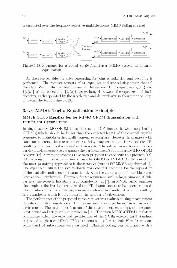
62 3 Link-Level Aspects
transmitted over the frequency-selective multiple-access MIMO fading channel.
Encoder InterleaverSymbolMapper
DeInterleaver Decoder Interleaver
Equalizer/
λ1(n)
ζ1(n)
b1(n)
b1(n)
DeInterleaver Decoder InterleaverλU(n)
ζU (n)
bU (n)
Encoder InterleaverSymbolMapper
bU (n)
Demapper
Figure 3.18: Structure for a coded single-/multi-user MIMO system with turboequalization.
At the receiver side, iterative processing for joint equalization and decoding isperformed. The receiver consists of an equalizer and several single-user channeldecoders. Within the iterative processing, the extrinsic LLR sequences {λu(n)} and{ζu(n)} of the coded bits {bu(n)} are exchanged between the equalizer and bothdecoders, each separated by the interleaver and deinterleaver in their iteration loop,following the turbo principle [2].
3.4.3 MMSE Turbo Equalization Principles
MMSE Turbo Equalization for MIMO OFDM Transmission withInsufficient Cyclic Prefix
In single-user MIMO-OFDM transmissions, the CP, located between neighboringOFDM symbols, should be longer than the expected length of the channel impulseresponse, to maintain orthogonality among sub-carriers. However, in channels withsome far clusters, the maximum excess delay may exceed the length of the CP,resulting in a loss of sub-carriers’ orthogonality. The related inter-block and inter-carrier interference severely degrades the performance of the standard MIMO-OFDMreceiver [12]. Several approaches have been proposed to cope with this problem [13],[14]. Among all these equalization schemes for OFDM and MIMO-OFDM, one of thethe most promising approaches is the iterative (turbo) SC-MMSE equalizer of [6].The equalizer utilizes the soft feedback from channel decoding for the separationof the spatially multiplexed streams jointly with the cancellation of inter-block andinter-carrier interference. However, for transmissions with a large number of sub-carriers, the receiver has still a high complexity. In [7], an MMSE turbo equalizerthat exploits the banded structure of the FD channel matrices has been proposed.The equalizer in [7] uses a sliding window to enforce this banded structure, resultingin a complexity which is only linear in the number of sub-carriers.
The performance of the proposed turbo receiver was evaluated using measurementdata-based off-line simulations. The measurements were performed in a macro cellenvironment. The major specifications of the measurement campaign, the measure-ment device and setup are summarized in [15]. The main MIMO-OFDM simulationparameters follow the extended specification of the 5 GHz wireless LAN standardin [16]. A single-user MIMO-OFDM transmission (U = 1) with K = M = 2 an-tennas and 64 sub-carriers were assumed. Channel coding was performed with a

3.4 MMSE-based Turbo Equalization Principles 63
(a)
0 2 4 6 8 10 1210
−5
10−4
10−3
10−2
10−1
100
SNR per antenna [dB]
BE
R
rec.#1, q = 0rec.#1, q = 4rec.#1, q = 8rec.#2
(b)
Figure 3.19: (a) Complementary CDF of channel delay spread (τrms) for different po-sitions of the measurement route. (b) BER performance versus averageEb/N0 for the measured channel at position Rx19, 16-QAM transmis-sion.
rate-1/2 convolutional code. The OFDM symbol duration was set to TS = 4μs andthe length of the cyclic prefix to Tc = 0.8μs.
Figure 3.19 (a) shows the complementary cumulative probability density function(CDF) of the root-mean-squared channel delay spread for different positions of themeasurement route. As observed from Fig. 3.19 (a), the delay spreads at positionRx19 are significantly large and exceed in some cases the length of the cyclic prefixof the MIMO-OFDM system, compared to other locations.
The BER performance of the proposed turbo receiver at location Rx19, referred toas ’rec. #1’ for different values of the FD window length q is shown in Fig. 3.19 (b).As a reference the BER performance of the conventional MIMO-OFDM receiver(q = 0) and the non-banded SC-MMSE turbo receiver, referred to as ’rec. #2’, arealso shown. It can be seen that with q = 8, the performance of the banded SC-MMSE turbo equalizer is very close to the non-banded turbo equalizer. Thus, theproposed technique works with properly chosen q values even in environments withrelatively large channel delay spreads.
Hybrid MMSE Turbo Equalization
The SC-MMSE turbo detector in [3], [6] achieves excellent performance in frequency-selective spatially-uncorrelated Rayleigh multiple-access fading channels. However,the performance of the detector drops significantly in scenarios where the users’channels are spatially correlated [9]. In [9], a hybrid turbo detection approach basedon group-wise SC-MMSE filtering combined with MAP signal detection for OFDMmulti-user systems has been proposed. The technique in [9], referred to as Hy SC-MMSE-MAP turbo detection, offers a design flexibility in terms of complexity incomputation and robustness against spatial correlation of the users’ channels.
The Hy SC-MMSE-MAP detector separates the U users into H disjoint groups{G1, G2, ..., GH}, such that each group contains Gh integers corresponding to user
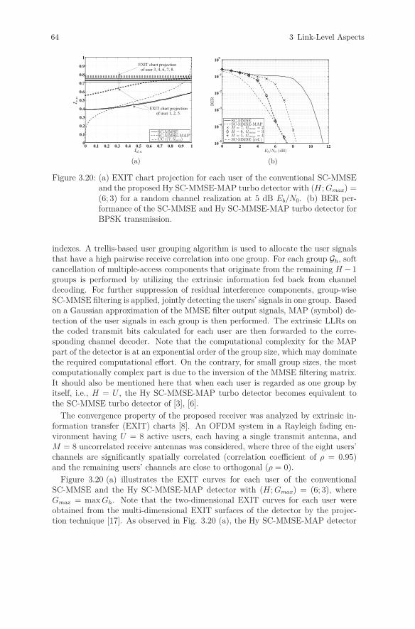
64 3 Link-Level Aspects
0 0.1 0.2 0.3 0.4 0.5 0.6 0.7 0.8 0.9 10
0.1
0.2
0.3
0.4
0.5
0.6
0.7
0.8
0.9
1
Id,n
I e,n
SC-MMSESC-MMSE-MAPCC ([7, 5]oct)
EXIT chart projectionof user 3, 4, 6, 7, 8.
EXIT chart projectionof user 1, 2, 5.
(a)
0 2 4 6 8 10 1210
−5
10−4
10−3
10−2
10−1
100
Eb/N0 (dB)
BE
R
SC-MMSESC-MMSE-MAPH = 7, Gmax = 2H = 6, Gmax = 3H = 5, Gmax = 4SC-MMSE (ref.)
(b)
Figure 3.20: (a) EXIT chart projection for each user of the conventional SC-MMSEand the proposed Hy SC-MMSE-MAP turbo detector with (H ; Gmax) =(6; 3) for a random channel realization at 5 dB Eb/N0. (b) BER per-formance of the SC-MMSE and Hy SC-MMSE-MAP turbo detector forBPSK transmission.
indexes. A trellis-based user grouping algorithm is used to allocate the user signalsthat have a high pairwise receive correlation into one group. For each group Gh, softcancellation of multiple-access components that originate from the remaining H − 1groups is performed by utilizing the extrinsic information fed back from channeldecoding. For further suppression of residual interference components, group-wiseSC-MMSE filtering is applied, jointly detecting the users’ signals in one group. Basedon a Gaussian approximation of the MMSE filter output signals, MAP (symbol) de-tection of the user signals in each group is then performed. The extrinsic LLRs onthe coded transmit bits calculated for each user are then forwarded to the corre-sponding channel decoder. Note that the computational complexity for the MAPpart of the detector is at an exponential order of the group size, which may dominatethe required computational effort. On the contrary, for small group sizes, the mostcomputationally complex part is due to the inversion of the MMSE filtering matrix.It should also be mentioned here that when each user is regarded as one group byitself, i.e., H = U , the Hy SC-MMSE-MAP turbo detector becomes equivalent tothe SC-MMSE turbo detector of [3], [6].
The convergence property of the proposed receiver was analyzed by extrinsic in-formation transfer (EXIT) charts [8]. An OFDM system in a Rayleigh fading en-vironment having U = 8 active users, each having a single transmit antenna, andM = 8 uncorrelated receive antennas was considered, where three of the eight users’channels are significantly spatially correlated (correlation coefficient of ρ = 0.95)and the remaining users’ channels are close to orthogonal (ρ = 0).
Figure 3.20 (a) illustrates the EXIT curves for each user of the conventionalSC-MMSE and the Hy SC-MMSE-MAP detector with (H ; Gmax) = (6; 3), whereGmax = max Gh. Note that the two-dimensional EXIT curves for each user wereobtained from the multi-dimensional EXIT surfaces of the detector by the projec-tion technique [17]. As observed in Fig. 3.20 (a), the Hy SC-MMSE-MAP detector
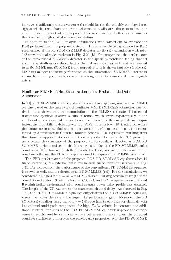
3.4 MMSE-based Turbo Equalization Principles 65
improves significantly the convergence threshold for the three highly correlated usersignals which stems from the group selection that allocates those users into onegroup. This indicates that the proposed detector can achieve better performance inthe presence of high spatial channel correlation.
In addition to the EXIT analysis, simulations were carried out to evaluate theBER performance of the proposed detector. The effect of the group size on the BERperformance of the Hy SC-MMSE-MAP detector for BPSK transmission with rate-1/2 convolutional codes is shown in Fig. 3.20 (b). For comparison, the performanceof the conventional SC-MMSE detector in the spatially-correlated fading channeland in a spatially-uncorrelated fading channel are shown as well, and are referredto as SC-MMSE and SC-MMSE (ref), respectively. It is shown that Hy SC-MMSE-MAP can achieve the same performance as the conventional SC-MMSE detector inuncorrelated fading channels, even when strong correlation among the user signalsexists.
Nonlinear MMSE Turbo Equalization using Probabilistic DataAssociation
In [11], a FD SC-MMSE turbo equalizer for spatial multiplexing single-carrier MIMOsystems based on the framework of nonlinear MMSE (NMMSE) estimation was de-rived. It is shown that the computation of the NMMSE estimate of the codedtransmitted symbols involves a sum of terms, which grows exponentially in thenumber of sub-carriers and transmit antennas. To reduce the complexity in compu-tation, the probabilistic data association (PDA) filtering idea [18] is adopted, wherethe composite inter-symbol and multiple-access interference component is approxi-mated by a multivariate Gaussian random process. The expression resulting fromthis Gaussian approximation can be iteratively solved following the PDA principle.As a result, the structure of the proposed turbo equalizer, denoted as PDA FDSC-MMSE turbo equalizer in the following, is similar to the FD SC-MMSE turboequalizer of [10]. However, with the presented method, internal iterations within theequalizer following the PDA principle are used to improve the NMMSE estimates.
The BER performance of the proposed PDA FD SC-MMSE equalizer after 10turbo iterations, five internal iterations in each turbo iteration, is shown in Fig.3.21. For comparison, the performance of the conventional FD SC-MMSE equalizeris shown as well, and is referred to as FD SC-MMSE (ref). For the simulations, weconsidered a single-user K = M = 2 MIMO system utilizing constraint length threeconvolutional codes [19] with rates r = 7/8, 2/3, and 1/2. A spatially-uncorrelatedRayleigh fading environment with equal average power delay profile was assumed.The length of the CP was set to the maximum channel delay. As observed in Fig.3.21, the PDA FD SC-MMSE equalizer outperforms the FD SC-MMSE equalizer,where the larger the rate r the larger the performance gain. Moreover, the FDSC-MMSE equalizer using the rate r = 7/8 code fails to converge for channels withless channel multi-path components for high Eb/N0 values. In contrast, the addi-tional internal iterations of the PDA FD SC-MMSE equalizer improve the conver-gence threshold, and hence, it can achieve better performance. Thus, the proposedequalizer significantly improves the convergence properties over the FD SC-MMSE
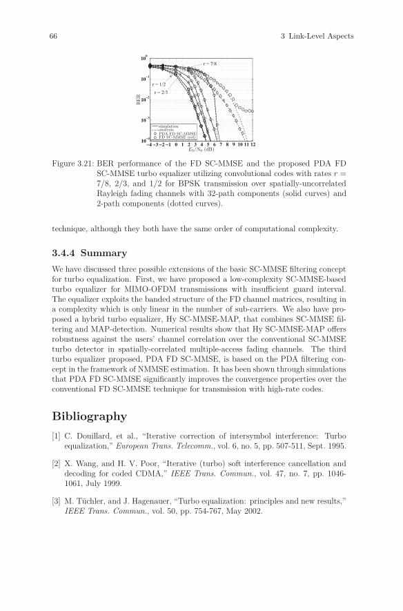
66 3 Link-Level Aspects
−4 −3 −2 −1 0 1 2 3 4 5 6 7 8 9 10 11 1210
−4
10−3
10−2
10−1
100
Eb/N0 (dB)
BE
R
simulationanalysisPDA FD SC-MMSEFD SC-MMSE (ref)
r = 1/2
r = 7/8
r = 2/3
Figure 3.21: BER performance of the FD SC-MMSE and the proposed PDA FDSC-MMSE turbo equalizer utilizing convolutional codes with rates r =7/8, 2/3, and 1/2 for BPSK transmission over spatially-uncorrelatedRayleigh fading channels with 32-path components (solid curves) and2-path components (dotted curves).
technique, although they both have the same order of computational complexity.
3.4.4 Summary
We have discussed three possible extensions of the basic SC-MMSE filtering conceptfor turbo equalization. First, we have proposed a low-complexity SC-MMSE-basedturbo equalizer for MIMO-OFDM transmissions with insufficient guard interval.The equalizer exploits the banded structure of the FD channel matrices, resulting ina complexity which is only linear in the number of sub-carriers. We also have pro-posed a hybrid turbo equalizer, Hy SC-MMSE-MAP, that combines SC-MMSE fil-tering and MAP-detection. Numerical results show that Hy SC-MMSE-MAP offersrobustness against the users’ channel correlation over the conventional SC-MMSEturbo detector in spatially-correlated multiple-access fading channels. The thirdturbo equalizer proposed, PDA FD SC-MMSE, is based on the PDA filtering con-cept in the framework of NMMSE estimation. It has been shown through simulationsthat PDA FD SC-MMSE significantly improves the convergence properties over theconventional FD SC-MMSE technique for transmission with high-rate codes.
Bibliography
[1] C. Douillard, et al., “Iterative correction of intersymbol interference: Turboequalization,” European Trans. Telecomm., vol. 6, no. 5, pp. 507-511, Sept. 1995.
[2] X. Wang, and H. V. Poor, “Iterative (turbo) soft interference cancellation anddecoding for coded CDMA,” IEEE Trans. Commun., vol. 47, no. 7, pp. 1046-1061, July 1999.
[3] M. Tüchler, and J. Hagenauer, “Turbo equalization: principles and new results,”IEEE Trans. Commun., vol. 50, pp. 754-767, May 2002.
Bibliography 67
[4] T. Abe, and T. Matsumoto, “Space-time turbo equalization in frequency-selective MIMO channels,” IEEE Trans. Veh. Techn., vol. 52, no. 3, pp. 469-475,May 2003.
[5] K. Fang, L. Rugini, and G. Leus, “Low-complexity block turbo equalization forOFDM systems with time-varying channels,” IEEE Trans. Signal Process., vol.56, pp. 5555-5566, Nov. 2008.
[6] C. Schneider, M. Grossmann, and R. S. Thomä, “Measurement based perfor-mance evaluation of MIMO-OFDM with turbo-equalization,” in Proc. IEEEVTC2005 Spring, Stockholm, Sweden, June 2005.
[7] M. Grossmann, C. Schneider, and R. Thomä, “Turbo equalization for MIMO-OFDM transmission with insufficient guard interval,” International Zurich Sem-inar on Communications, Zurich, Switzerland, pp. 114-117 , Feb. 2006.
[8] S. ten Brink, “Convergence behavior of iteratively decoded parallel concatenatedcodes,” IEEE Trans. Commun., vol. 49, no. 10, pp. 1727-1737, Oct. 2001.
[9] M. Grossmann, and T. Matsumoto, “Hybrid turbo multiuser detection forOFDM transmission with spatially-correlated channels,” IEEE Commun. Let-ters, vol. 11, pp. 420-422, May 2007.
[10] K. Kansanen, and T. Matsumoto, “An analytical method for MMSE MIMOturbo equalizer EXIT chart computation,” IEEE Trans. Wireless Commun., vol.6, no. 1, pp. 59-63, Jan. 2007.
[11] M. Grossmann, and T. Matsumoto, “Nonlinear Frequency Domain MMSETurbo Equalization using Probabilistic Data Association,” IEEE Commun. Let-ters, vol. 12, pp. 295-297, April 2008.
[12] G.L. Stüber et al., “Broadband MIMO-OFDM wireless communications,” Pro-ceedings of the IEEE, vol. 92, no. 2, pp. 271-294, Feb 2004.
[13] D. Kim, and G.L. Stüber, “Residual ISI cancellation for OFDM with applicationto HDTV broadcasting,” IEEE J. Select. Areas Commun., vol. 16, pp. 1590-1599,Oct. 1998.
[14] G. Leus, and M. Moonen, “Per-Tone equalization for MIMO OFDM systems,”IEEE Trans. Signal Process., vol. 51, pp. 2965-2975, Nov. 2003.
[15] M. Landmann et al., “Polarisation Behaviour of Discrete Multipath and DiffuseScattering in Urban Environments at 4.5GHz,”EURASIP Journal on WirelessCommunications and Networking, Special Issue on Space-Time Channel Model-ing for Wireless Communications and Networking, Article ID 57980, 16 pages,Jan 2007.
[16] IEEE Standard 802.11a-1999, “High-speed physical layer in the 5 GHz band,”1999.

68 3 Link-Level Aspects
[17] F. Brännström et al., “Convergence analysis and optimal scheduling for multipleconcatenated codes,” IEEE Trans. Inform. Theory, vol. 51, pp. 3354-3364, Sept.2005.
[18] J. Luo et al., “Near Optimal Multiuser Detection in Synchronous CDMA usingProbabilistic Data Association,” IEEE Comm. Letters, vol. 5, no. 9, pp. 361-363,Sep. 2001.
[19] J. G. Proakis, “Digital Communications,” 4th ed. New York: McGraw-Hill,2001.
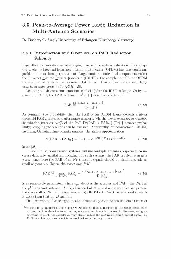
3.5 Peak-to-Average Power Ratio Reduction 69
3.5 Peak-to-Average Power Ratio Reduction in
Multi-Antenna Scenarios
R. Fischer, C. Siegl, University of Erlangen-Nürnberg, Germany
3.5.1 Introduction and Overview on PAR ReductionSchemes
Regardless its considerable advantages, like, e.g., simple equalization, high adap-tivity, etc., orthogonal frequency-divsion multiplexing (OFDM) has one significantproblem: due to the superposition of a large number of individual components withinthe (inverse) discrete Fourier transform ((I)DFT), the complex amplitude OFDMtransmit signal tends to be Gaussian distributed. Hence it exhibits a very largepeak-to-average power ratio (PAR) [29].
Denoting the discrete-time transmit symbols (after the IDFT of length D) by ak,k = 0, . . . , D − 1, the PAR is defined as1 (E{·} denotes expectation)
PARdef=
maxk=0,...,D−1 |ak|2E{|ak|2} (3.22)
As common, the probability that the PAR of an OFDM frame exceeds a giventhreshold PARth serves as performance measure. Via the complementary cumulativedistribution function (ccdf) of the PAR Pr{PAR > PARth} (Pr{·} denotes proba-bility), clipping probabilities can be assessed. Noteworthy, for conventional OFDM,assuming Gaussian time-domain samples, the simple approximation
Pr{PAR > PARth} = 1 − (1 − e−PARth)D ≈ D e−PARth (3.23)
holds [28].Future OFDM transmission systems will use multiple antennas, especially to in-
crease data rate (spatial multiplexing). In such systems, the PAR problem even getsworse, since here the PAR of all NT transmit signals should be simultaneously assmall as possible. Hence, the worst-case PAR
PARdef= max
μ=1,...,NT
PARμ =maxμ=1,...,NT, k=0,...,D−1 |aμ,k|2
E{|a2μ,k} . (3.24)
is as reasonable parameter, where aμ,k denotes the samples and PARμ the PAR atthe μth transmit antenna. As NTD instead of D time-domain samples are presentthe same ccdf of PAR as in (single-antenna) OFDM with NTD carriers results, whichis worse than that for D carriers.
The occurrence of large signal peaks substantially complicates implementation of
1We consider a standard discrete-time OFDM system model. Insertion of the cyclic prefix, pulseshaping, and modulation to radio frequency are not taken into account. However, using anoversampled DFT, the samples ak very closely reflect the continuous-time transmit signal [45,46, 58] and hence are sufficient to assess PAR reduction algorithms.
70 3 Link-Level Aspects
the analog radio frequency frontend at the transmitter side since amplifiers operatinglinearly over a wide dynamic range have to be employed. Undeliberate clipping ofpeaks by non-linear amplifiers will, on the one hand, cause signal distortion andhence lower the power efficiency of the transmission system. On the other hand,and even more critical, any non-linear operation on the continuous-time transmitsignal will cause intolerable out-of-band radiation which, in the last resort, may leadto a violation of spectral masks imposed by standards bodies.
The obvious solution to this problem would be to operate the amplifiers withsufficiently large power back-offs. This, however, also leads to very power-inefficienttransmission systems. A much more preferable answer to the PAR problem of OFDMis to apply some algorithmic control to the transmit signal. Basically, the idea ofPAR reduction schemes is to only generate OFDM frames with low, or at leasttolerable PAR.
Since the mid 1990s, a variety of PAR reduction algorithms has been developed.Even though they are all based on (i) introducing new degrees of freedom for restric-tion to or selection of suited candidate OFDM signals and (ii) implicitly or explicitlyadding redundancy, very different approaches are present in literature. The mostrelevant (among others) PAR reduction principles are (for a more detailed overviewsee, e.g., [33]):
Redundant Signal Representations: Multiple transmit signals are createdwhich represent the given data. From that the “best” representation is selected.Here, in particular selected mapping (SLM), e.g., [2, 27, 28, 30, 47, 57] and partialtransmit sequences (PTS), e.g., [8, 24, 31, 48] have to be mentioned.
Tone Reservation: Here, some carriers are not used for data transmission butare selected via an algorithmic search, e.g., [41, 54].
Clipping (and Filtering): The transmit signal is passed through a non-linear,memoryless device. Combinations of clipping and filtering are also popular, e.g.,[26, 43, 50, 51].
Constellation Expansion: The signal constellations in the carriers are warped;deviations from the regular QAM grid are allowed, especially for points at theperimeter of the constellation, e.g., [40].
Coding Techniques: Here, an algebraic code construction over the carriers isused, e.g., [34, 38, 52, 53] to exclude undesired frames.
(Trellis) Shaping Techniques: Employing a signal shaping algorithm operatingover the frequency domain symbols, the signal envelope can be influenced, e.g.,[35, 44, 49].
When additionally employing multi-antenna or multiple-input/multiple-output(MIMO) techniques, PAR reduction methods tailored to this situation should beutilized, instead of simply performing single-antenna PAR reduction in parallel, asdone, e.g., in [27]. The fundamental idea behind PAR reduction in MIMO OFDMcan be paraphrased with “redistributing the peak power over the antennas”. Thegain of MIMO PAR reduction is an increased slope of the ccdf curves, i.e., theprobability of occurrence of large signal peaks can significantly lowered compared tosingle-antenna schemes. In this regard, MIMO approaches show a similar behavioras do MIMO techniques with respect to error rate: the slope of the respectiveperformance curves is increased; some kind of diversity gain is achieved.
3.5 Peak-to-Average Power Ratio Reduction 71
In this chapter, the main ideas and algorithms for MIMO PAR reduction willbe reviewed and the achievable gains over single-antenna techniques will be brieflydiscussed.
3.5.2 PAR Reduction Schemes for MIMO Transmission
In this section, we give an overview over PAR reduction schemes for MIMO trans-mission. Thereby, we have to distinguish two basic scenarios: on the one hand, weconsider point-to-point MIMO transmission achieving spectral multiplexing gain,where the signals can be processed jointly at transmitter and receiver. On the otherhand, variants for the point-to-multipoint situation, i.e., the broadcast channel, wherejoint signal processing is only possible at the transmitter side are briefly discussed.In the multipoint-to-point scenario (multiple-access channel) no joint optimizationof the transmit signals can be performed, hence this case is not amenable for MIMOapproaches.
SLM- and PTS-Type PAR Reduction
Much work has been invested in generalizing the SLM principle [28] to the point-to-point MIMO setting, e.g., [2, 4, 5, 7, 9, 11, 12, 15, 18, 27, 42]. The extension of PTS toMIMO transmission is addressed in [8, 10].
Ordinary and simplified SLM
In ordinary SLM [27] SISO SLM is applied NT times in parallel. For each of theparallel OFDM frames the best mapping out of U possible is individually selected. Insimplified SLM a restriction to select the lth candidate over all antennas is imposed.In total, in both cases complexity per antenna is determined by the U IDFTs.
It can be shown that the asymptotic behavior of the ccdf is given const · e−PARth U ,which is the same as in single-antenna SLM. Both schemes do not achieve any MIMOgain.
Directed SLM
The first scheme, directed SLM, tailored to the MIMO situation has been presentedin [2,4]. Main idea is to invest complexity only where PAR reduction is really needed.Instead of performing U trials for each of the NT transmitters, the fixed budget ofNTU IDFTs (same as in ordinary SLM) is used to successively improve the currentlyhighest PAR over the antennas. Complexity is hence adaptively distributed over theantennas.
In the first step the PARs of the NT initial (original) OFDM frames are calculated.Then, in each successive step, the OFDM frame with instantaneously highest PARis considered. Calculating a next candidate, a reduction of PAR is tried. Thisprocedure is continued until the same number of IDFT and PAR calculations havebeen carried out.
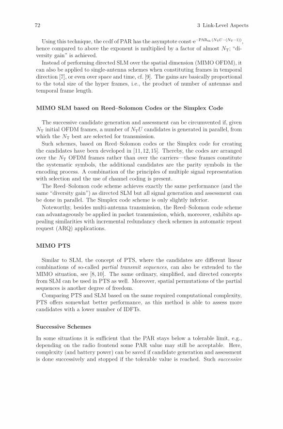
72 3 Link-Level Aspects
Using this technique, the ccdf of PAR has the asymptote const·e−PARth (NTU−(NT−1)),hence compared to above the exponent is multiplied by a factor of almost NT; “di-versity gain” is achieved.
Instead of performing directed SLM over the spatial dimension (MIMO OFDM), itcan also be applied to single-antenna schemes when constituting frames in temporaldirection [7], or even over space and time, cf. [9]. The gains are basically proportionalto the total size of the hyper frames, i.e., the product of number of antennas andtemporal frame length.
MIMO SLM based on Reed–Solomon Codes or the Simplex Code
The successive candidate generation and assessment can be circumvented if, givenNT initial OFDM frames, a number of NTU candidates is generated in parallel, fromwhich the NT best are selected for transmission.
Such schemes, based on Reed–Solomon codes or the Simplex code for creatingthe candidates have been developed in [11, 12, 15]. Thereby, the codes are arrangedover the NT OFDM frames rather than over the carriers—these frames constitutethe systematic symbols, the additional candidates are the parity symbols in theencoding process. A combination of the principles of multiple signal representationwith selection and the use of channel coding is present.
The Reed–Solomon code scheme achieves exactly the same performance (and thesame “diversity gain”) as directed SLM but all signal generation and assessment canbe done in parallel. The Simplex code scheme is only slightly inferior.
Noteworthy, besides multi-antenna transmission, the Reed–Solomon code schemecan advantageously be applied in packet transmission, which, moreover, exhibits ap-pealing similarities with incremental redundancy check schemes in automatic repeatrequest (ARQ) applications.
MIMO PTS
Similar to SLM, the concept of PTS, where the candidates are different linearcombinations of so-called partial transmit sequences, can also be extended to theMIMO situation, see [8, 10]. The same ordinary, simplified, and directed conceptsfrom SLM can be used in PTS as well. Moreover, spatial permutations of the partialsequences is another degree of freedom.
Comparing PTS and SLM based on the same required computational complexity,PTS offers somewhat better performance, as this method is able to assess morecandidates with a lower number of IDFTs.
Successive Schemes
In some situations it is sufficient that the PAR stays below a tolerable limit, e.g.,depending on the radio frontend some PAR value may still be acceptable. Here,complexity (and battery power) can be saved if candidate generation and assessmentis done successively and stopped if the tolerable value is reached. Such successive

3.5 Peak-to-Average Power Ratio Reduction 73
PAR reduction schemes have been proposed in [16, 19, 23] and already mentionedin [4].
Given the tolerable PAR, PARtol, the average number of assessed candidates canbe calculated. Main result is that this number is simply given by the inverseof the cdf of PAR of the underlying original OFDM scheme, i.e., n = 1/(1 −Pr{PAR > PARtol}), which using the Gaussian approximation calculates to n =(1 − e−PARtol)−D. Noteworthy, for PARtol equal to the so-called “critical PAR value”PARtol = log(D) (cf., e.g., [59]) and reasonably large number D of carriers, averagecomplexity amounts to only n = e = 2.71828 . . . (Euler’s number). Hence, us-ing successive PAR reduction approaches, on average only very low computationalcomplexity is required to achieve significant gains.
PAR Reduction for Downlink Transmission
Compared to PAR reduction in point-to-point MIMO systems, schemes applicablein point-to-multipoint scenarios (broadcast channel) are a much more challengingtask. Since no joint receiver side signal processing is possible, at the transmitterside only operation for candidate generation/modification can be applied which canindividually be reversed in each of the receivers.
Among the above discussed schemes, only simplified SLM can be used for thebroadcast channel. Consequently, adopted PAR reduction algorithms have beendeveloped [5,14]. The selected sorting technique uses the presence of the transmitterside pre-equalization, specifically, the application of (sorted) Tomlinson–Harashimaprecoding (THP) [32]. Modifying the order of the successive encoding in THP, whichis present in each carrier individually and which operates over the spatial (user)dimension, the PAR of the OFDM frames at the antenna array can be influenced.Since the choices of the ordering interact and the ordering in each carrier affectsall antenna signals, no directed or successive approach can be designed. In turn,in the broadcast case no diversity gain compared to single-antenna transmission ispossible.
Other Optimization Criteria
Besides PAR reduction, other optimization aims for OFDM transmission may beof interest, e.g., average transmit power, cubic metric, or out-of-band power. Ingeneral, the aim in future OFDM systems will be to generate signal with certaindesired properties. This deliberate generation of signals is commonly referred to assignal shaping [32]; PAR reduction is one particular instance thereof.
Concentrating on point-to-point MIMO systems, the extension of the above schemesto the more general aim of signal shaping is easily possible. Employing the SLMapproach of candidate generation and selection, due to this selection step any crite-rion of optimality can be taken into account. Therefore, the signal parameter to beoptimized has to be expressed mathematically, defining a selection metric.
Work on the optimization of other criteria than the PAR can be found in [3, 17],where out-of-band power reduction is aspired and power-amplifier-oriented metricshave been introduced. The even more general framework of probabilistic signalshaping in MIMO OFDM has been presented in [23].

74 3 Link-Level Aspects
Representation of Side Information
In most of the above discussed PAR reduction algorithms, the transmission of sideinformation to characterize the selected candidate / performed signal modification isrequired. Only with this knowledge, at the receiver the initial data can be recoveredfrom the received OFDM frame (by inverting the applied “mapping” used in SLM).The side information problem has been addressed, e.g., in [25, 36, 37, 39, 55, 56].However, up to now, only very few approaches, e.g. [30], exists in literature whereno explicit side information is necessary.
The embedding of explicit side information has been studied in [22], where itis shown that spending only a few carriers to represent the required redundancy issufficient to extract it with very high reliability and without noticeable deterioratingeffect on the error rate of the data bits. In [20,21] an implicit transmission of the sideinformation via rotations has been proposed. According to some defined pattern,the QAM constellations in the carrier are left as they are or rotated by 45◦. Noincrease in transmit power occurs, and the rotation pattern—directly representingthe side information bits—can be detected highly reliable with almost no additionaleffort.
3.5.3 Numerical Results
Figure 3.22 shows the PAR reduction performance of directed SLM in terms of theccdf. Various numbers NT of transmit antennas are studied. The ccdfs of the originalsignal (single- and multi-antenna case) and the one of ordinary SLM (individualparallel application of single-antenna SLM) serve as reference. Directed SLM (whichis as efficient as the Reed–Solomon code version) outperforms the individual parallelapplication of the respective PAR reduction scheme. The benefit of the directed/RScode approach is that its performance increases the more transmit antennas areused. In contrast to that, for the original signal or oSLM the PAR statistics getsworse with the number of transmit antennas. The benefit of directed SLM can alsobe observed by considering the asymptotic slopes (large PARth) of the ccdf curves.For single-antenna SLM, the slope of the ccdf of ordinary SLM is determined by thenumber U of a assessed signal candidates. Applying directed SLM offers an increaseof the slope by (approximately) a factor of NT, compared to ordinary SLM whenassessing the same total number of signal candidates. This effect is similar to thediversity order (slope of bit error rate curves) when considering digital transmissionover flat-fading MIMO channels.
3.5.4 Summary
Over the last years, the field of PAR reduction for OFDM has experienced a re-naissance. In particular PAR reduction in MIMO schemes has gained enormousinterest and a huge number of publications has appeared in journals and confer-ence proceedings. However, transferring the MIMO concepts back to single-antennatransmission—most simple by establishing hyper frames over time—new interestingschemes also for conventional OFDM have been designed. In the future, a still rapidgrowth of this research field is anticipated. In particular, the deliberate generation
3.5 Peak-to-Average Power Ratio Reduction 75
7 7.5 8 8.5 9 9.5 1010−5
10−4
10−3
10−2
10−1
100
10 log10 (PARth) [dB] −→
Pr{
PA
R>
PA
Rth}−→
original SISOoriginal MIMOSISO SLMoSLMdSLMNT = 2NT = 4NT = 8
Figure 3.22: Ccdf of PAR of ordinary and directed SLM; D = 512, M = 4, U = 16.
of OFDM signals exhibiting some desirable properties via signal shaping to adaptthe transmission systems even closely to the specific demands at hand is its veryinfancy.
Bibliography
Papers Emerged from the Project:
[1] R.F.H. Fischer, “Peak-to-Average Power Ratio (PAR) Reduction in OFDMbased on Lattice Decoding,” In Proceedings of the 11th Int. OFDM Workshop,pp. 71–75, Hamburg, Germany, August 2006.
[2] R.F.H. Fischer, M. Hoch, “Directed Selected Mapping for Peak-to-AveragePower Ratio Reduction in MIMO OFDM,” IEE Electronics Letters, Vol. 42,No. 22, pp. 1289–1290, October 2006.
[3] R.F.H. Fischer, C. Siegl, M. Hoch, “Out-of-Band Power Reduction in MIMOOFDM,” in Proceedings of International ITG/IEEE Workshop on Smart An-tennas, Vienna, Austria, February 2007.
[4] R.F.H. Fischer, M. Hoch, “Peak-to-Average Power Ratio Reduction in MIMOOFDM,” in Proceedings of the IEEE International Conference on Communica-tions, Glasgow, United Kingdom, June 2007.
[5] C. Siegl, R.F.H. Fischer, “Peak-to-Average Power Ratio Reduction in Multi-User OFDM,” in Proceedings of the International Symposium on InformationTheory 2007, Nice, France, June 2007.
76 3 Link-Level Aspects
[6] R.F.H. Fischer, “Widely-Linear Selected Mapping for Peak-to-Average PowerRatio Reduction in OFDM,” IEE Electronics Letters, Vol. 43, No. 14, pp. 766–767, July 2007.
[7] C. Siegl, R.F.H. Fischer, “Directed Selected Mapping for Peak-to-Average Po-wer Ratio Reduction in Single-Antenna OFDM,” in Proceedings of 12th Int.OFDM Workshop, Hamburg, Germany, August 2007.
[8] C. Siegl, R.F.H. Fischer, “Partial Transmit Sequences for Peak-to-AveragePower Ratio Reduction in Multi-Antenna OFDM,” EURASIP Journal on Wire-less Communications and Networking, Special Issue on “Multicarrier Systems”,Article ID 325829, 2008.
[9] C. Siegl, R.F.H. Fischer, “Joint Spatial and Temporal PAR Reduction in MIMOOFDM,” in International ITG Conference on Source and Channel Coding 2008,Ulm, Germany, January 2008.
[10] C. Siegl, R.F.H. Fischer, “Comparison of Partial Transmit Sequences and Se-lected Mapping for Peak-to-Average Power Ratio Reduction in MIMO OFDM,”in International ITG/IEEE Workshop on Smart Antennas, Darmstadt, Ger-many, February 2008.
[11] R.F.H. Fischer, C. Siegl, “Peak-to-Average Power Ratio Reduction in OFDMusing Reed-Solomon Codes,” in International Zurich Seminar 2008, pp. 40–43,Zurich, March 2008.
[12] R.F.H. Fischer, C. Siegl, “OFDM Peak-to-Average Power Ratio Reductionbased on the Simplex Code,” in Proceedings of the International Symposiumon Information Theory (ISIT 2008), Toronto, Canada, July 2008.
[13] C. Siegl, R.F.H. Fischer, “Tone Reservation for Peak-to-Average Power RatioReduction in OFDM under Different Optimization Constraints,” in Proceedingsof 13th International OFDM Workshop, Hamburg, Germany, August 2008.
[14] C. Siegl, R.F.H. Fischer, “Selected Sorting for PAR Reduction in OFDM Multi-User Broadcast Scenarios,” in Proceedings of International ITG Workshop onSmart Antennas (WSA 2009), Berlin, Germany, February 2009.
[15] R.F.H. Fischer, C. Siegl, “Reed-Solomon and Simplex Codes for Peak-to-Average Power Ratio Reduction in OFDM,” IEEE Transactions on InformationTheory, Vol. 55, No. 4, pp. 1519–1528, April 2009.
[16] R.F.H. Fischer, C. Siegl, “Successive PAR Reduction in (MIMO) OFDM,” inProceedings of the IEEE International Conference on Communications (ICC2009), Dresden, Germany, June 2009.
[17] C. Siegl, R.F.H. Fischer, “Out-of-Band Power Reduction using Selected Map-ping with Power-Amplifier-Oriented Metrics,” in Proceedings of 14th Interna-tional OFDM Workshop, Hamburg, Germany, September 2009.
Bibliography 77
[18] R.F.H. Fischer, C. Siegl, “Peak-to-Average Power Ratio Reduction in Single-and Multi-Antenna OFDM via Directed Selected Mapping,” IEEE Transactionson Communications, Vol. 11, No. 11, pp. 3205–3208, November 2009.
[19] C. Siegl, R.F.H. Fischer, “Asymptotic Performance Analysis and SuccessiveSelected Mapping for PAR Reduction in OFDM,” IEEE Transactions on SignalProcessing, August 2009. Accepted for publication.
[20] C. Siegl, R.F.H. Fischer, “Selected Mapping with Implicit Transmission of SideInformation using Discrete Phase Rotations,” in International ITG Conferenceon Source and Channel Coding, Siegen, Germany, January 2010.
[21] C. Siegl, R.F.H. Fischer, “Transmission and Detection of Side Informationfor Selected Mapping in MIMO OFDM,” in Proceedings of International ITGWorkshop on Smart Antennas (WSA 2010), Bremen, Germany, February 2010.
[22] C. Siegl, R.F.H. Fischer, “Selected Mapping with Explicit Transmission of SideInformation,” in IEEE Wireless Communications and Networking Conference,Sydney, Australia, April 2010.
[23] R.F.H. Fischer, C. Siegl, “Probabilistic Signal Shaping in MIMO OFDM,”Submitted for Publication, Mai 2009.
Other References:
[24] A. Alavi, C. Tellambura, I. Fair, “PAPR Reduction of OFDM Signals UsingPartial Transmit Sequence: An Optimal Approach Using Sphere Decoding,”IEEE Communications Letters, pp. 982–984, Nov. 2005.
[25] E. Alsusa, L. Yang, “Redundancy-free and BER-Maintained Selective Mappingwith Partial Phase-Randomising Sequences for Peak-to-Average Power RatioReduction in OFDM Systems,” IET Communications, pp. 66-–74, January2008.
[26] J. Armstrong, “Peak-to-Average Power Reduction for OFDM by RepeatedClipping and Frequency Domain Filtering,” Electronics Letters, pp. 246–247,Feb. 2002.
[27] M.-S. Baek, M.-J. Kim, Y.-H. You, H.-K. Song, “Semi-Blind Channel Estima-tion and PAR Reduction for MIMO-OFDM System With Multiple Antennas,”IEEE Transactions on Broadcasting, pp. 414–424, Dec. 2004.
[28] R. Bäuml, R.F.H. Fischer, J.B. Huber, “Reducing the Peak-to-Average PowerRatio of Multicarrier Modulation by Selected Mapping,” Electronics Letters,pp. 2056–2057, Oct. 1996.
[29] J.A.C. Bingham, “Multicarrier Modulation for Data Transmission: An IdeaWhose Time Has Come,” IEEE Communications Magazine, pp. 5–14, May1990.
78 3 Link-Level Aspects
[30] M. Breiling, S. Müller–Weinfurtner, J.B. Huber, “SLM Peak-Power Reductionwithout Explicit Side Information,” IEEE Communications Letters, pp. 239–241, June 2001.
[31] L.J. Cimini, N.R. Sollenberger, “Peak-to-Average Power Ratio Reduciton ofan OFDM signal using Partial Transmit Sequences,” IEEE CommunicationsLetters, pp. 86–88, Mar. 2000.
[32] R.F.H. Fischer, Precoding and Signal Shaping for Digital Transmission, JohnWiley & Sons, Inc., New York, 2002.
[33] S.H. Han, J.H. Lee, “An Overview of Peak-to-Average Power Ratio ReductionTechniques for Multicarrier Transmission,” IEEE Wireless Communications,pp. 56–65, April 2005.
[34] W. Henkel, “Analog Codes for Peak-to-Average Ratio Reduction,” ITG Conf.on Source and Channel Coding, pp. 151–155, Munich, Jan. 2000.
[35] W. Henkel, B. Wagner, “Another Application for Trellis Shaping: PAR Reduc-tion for DMT (OFDM),” IEEE Transactions on Communications, pp. 1471–1476, Sep. 2000.
[36] A.D.S. Jayalath, C. Tellambura, “A blind SLM receiver for PAR-reducedOFDM,” in IEEE Vehicular Technology Conference (VTC 2002-Fall), pp. 219–222, Sept. 2002.
[37] A.D.S. Jaylath, C. Tellambura, “SLM and PTS Peak-Power Reduction ofOFDM Signals Without Side Information,” IEEE Transactions on WirelessCommunications, Vol. 4, No. 5, pp. 2006-–2013, Sept. 2005.
[38] A.E. Jones, T.A. Wilkinson, S.K. Barton, “Block Coding Scheme for Reductionof Peak to Mean Envelope Power Ratio of Multicarrier Transmission Scheme,”Electronics Letters, pp. 2098–2099, Dec. 1994.
[39] B.K. Khoo, S.Y. Le Goff, C.C. Tsimendidis, B.S. Sharif, “OFDM PAPR Reduc-tion Using Selected Mapping Without Side Information,” in IEEE InternationalConference on Communications (ICC 2007), Glasgow, United Kingdom, June2007.
[40] B.S. Krongold, D.L. Jones, “PAR Reduction in OFDM via Active ConstellationExtension,” IEEE Transactions Broadcasting, pp. 258–268, Sep. 2003.
[41] B.S. Krongold, D.L. Jones, “An active-set approach for OFDM PAR reductionvia tone reservation,” IEEE Transactions on Signal Processing, pp. 495–509,Feb. 2004.
[42] Y.-L. Lee, Y.-H. You, W.-G. Jeon, J.-H. Paik, H.-K. Song, “Peak-to-AveragePower Ratio in MIMO-OFDM Systems Using Selective Mapping,” IEEE Com-munications Letters, pp. 575–577, Dec. 2003.
Bibliography 79
[43] X. Li, L.J. Cimini, “Effect of Clipping and Filtering on the Performance ofOFDM,” IEEE Communications Letters, pp. 131–133, May 1998.
[44] M. Litzenburger, W. Rupprecht, “Combined Trellis Shaping and Coding toControl the Envelope of a Bandlimited PSK-Signal,” in IEEE InternationalConference on Communications (ICC ’94), pp. 630–634, May 1994.
[45] S. Litsyn, G. Wunder, “Generalized Bounds on the Crest-Factor Distributionof OFDM Signals With Application to Code Design,” IEEE Transactions onInformation Theory, pp. 992–1006, March 2006.
[46] S. Litsyn, Peak Power Control in Multicarrier Communications, CambridgeUniversity Press, Cambridge, 2007.
[47] S.H. Müller, R.W. Bäuml, R.F.H. Fischer, J.B. Huber, “OFDM with ReducedPeak-to-Average Power Ratio by Multiple Signal Representation,” Annal ofTelecommunications, pp. 58–67, Feb. 1997.
[48] S.H. Müller, J.B. Huber, “OFDM with Reduced Peak-to-Average Power Ratioby Optimum Combination of Partial Transmit Sequences,” Electronics Letters,Vol. 33, pp. 368–369, Feb. 1997.
[49] T.T. Nguyen, L. Lampe, “On Trellis Shaping for PAR Reduction in OFDMSystems,” IEEE Transactions on Communications, pp. 1678–1682, Sep. 2007.
[50] R. O’Neill, L.B. Lopes, “Envelope Variations and Spectral Splatter in ClippedMulticarrier Signals,” in IEEE International Symposium on Personal, Indoorand Mobile Radio Communications (PIMRC ’95), Toronto, Canada, pp. 71–75,Sep. 1995.
[51] M. Pauli, “Zur Anwendung des Mehrträgerverfahrens OFDM mit reduzierterAußerbandstrahlung im Mobilfunk,” Ph.D. dissertation, University Hannover,1999.
[52] K.-U. Schmidt, “On Cosets of the Generalized First-Order Reed-Muller Codewith low PMEPR,” IEEE Transactions on Information Theory, pp. 3220–3232,July 2006.
[53] K.-U. Schmidt, “Complementary Sets, Generalized Reed-Muller Codes, andPower Control for OFDM,” IEEE Transactions on Information Theory,pp. 808–814, Feb. 2007.
[54] J. Tellado, Peak to Average Power Reduction for Multicarrier Modulation.Ph.D. dissertation, Stanford University, 2000.
[55] G.R. Tsouri, D. Wulich, “Efficient Coding of Side Information for Selected Map-ping PAPR Reduction,” in Wireless Telecommunications Symposium (WTS2008), pp. 286–290, April 2008.

80 3 Link-Level Aspects
[56] A. Vallavaraj, B.G. Stewart, D.K. Harrison, F.G. McIntosh, “Reducing thePAPR of OFDM Using a Simplified Scrambling SLM Technique with No Ex-plicit Side Information,” in IEEE International Conference on Parallel andDistributed Systems (ICPADS ’08), pp. 902–907, Dec. 2008.
[57] P. Van Eetvelt, G. Wade, M. Tomlinson, “Peak to average power reduction forOFDM schemes by selective scrambling,” Electronics Letters, Vol. 32, pp. 1963–1964, Oct. 1996.
[58] G. Wunder, H. Boche, “Peak value estimation of bandlimited signals from theirsamples, noise enhancement, and a local characterization in the neighborhoodof an extremum,” IEEE Transactions on Signal Processing, pp. 771–780, March2003.
[59] G. Wunder, H. Boche, “Upper Bounds on the Statistical Distribution of theCrest-Factor in OFDM Transmission,” IEEE Transactions on Information The-ory, pp. 488–494, Feb. 2003.
3.6 Single- vs. Multicarrier Transmission 81
3.6 Single- vs. Multicarrier Transmission in
MIMO and Multiuser Scenarios
R. Fischer, C. Stierstorfer, University of Erlangen-Nürnberg, Germany
3.6.1 Introduction
Since the invention of orthogonal frequency-division multiplexing (OFDM), the ques-tion has arisen whether multicarrier (MC) or singlecarrier modulation is superior orpreferable over the competitor. In [25, 36] it has been shown, that in principleOFDM and singlecarrier pulse amplitude modulation (PAM) with decision-feedbackequalization (DFE) can achieve the same transmission rate and both can utilize thecapacity of the underlying channel (cf. also [22, 29]).
Since the fundamental insight (e.g., [28,30]) that by using antenna arrays in trans-mitter and receiver, hence creating a multiple-input/multiple-output (MIMO) chan-nel, spectral efficiency and thus data rate can dramatically be increased, this questionhas been posed again: is MIMO OFDM or singlecarrier MIMO the better choice?Moreover, this comparison is not only of interest in point-to-point MIMO (multi-antenna) transmission, but as well for multipoint-to-point scenarios (multiple accessproblem, uplink) and for point-to-multipoint scenarios (broadcast channel, down-link), when the transmission paths exhibit intersymbol interference (ISI) and thuscall for some kind of equalization.
In this chapter, we briefly compare single- and multicarrier MIMO transmissionwith respect to the achievable performance. Besides the study of information- andcommunication-theoretical bounds, the consequences on the code design when em-ploying practical channel coding schemes are discussed, too.
3.6.2 Point-to-Point MIMO Transmission
In this section, we concentrate on point-to-point MIMO transmission, e.g., usingantenna arrays in both transmitter and receiver, each with NT antennas. Whenconsidering transmission over MIMO ISI channels, two sources of (self) interferenceoccur: interference of the parallel data streams (spatial or multi-user interference(MUI)) and intersymbol (temporal) interference. The possible equalization schemescan be characterized by how they deal with these two types of interferences.
The first approach for transmission over MIMO ISI channels is to treat MUI andISI jointly, i.e., to perform combined spatial/temporal equalization. An attractivescheme is DFE over space and time (MIMO DFE), see [27]. Here, by applying afeedforward filter, the end-to-end impulse response is shaped such that it exhibitsspatial and temporal causality, i.e., symbols transmitted at some time instant shouldonly interfere with receive symbols at subsequent time instances and symbols trans-mitted at the same time instance over the antennas should also only interfere withreceive symbols for antennas with larger labels (spatial/temporal causality). Then,the symbols are processed in a zig-zag fashion over space and time, taking alreadydetected symbols (via feedback) into account. Neglecting error propagation in the

82 3 Link-Level Aspects
feedback loop, MIMO DFE decouples the MIMO ISI channel into a set of NT par-allel (near AWGN) channels with individual signal-to-noise ratios. Details on thisMIMO DFE can be found in [1, 27].
The competing approach is to treat MUI and ISI separately. In MIMO systemstemporal equalization can be performed by applying an OFDM transmitter andOFDM receiver (using a (inverse) discrete Fourier transform ((I)DFT) of length D)to each transmit and receive antenna, respectively. Thereby, the MIMO ISI channelis decomposed into a set of D independent flat fading MIMO channels. Then, foreach of this parallel flat fading MIMO channels (the tones), spatial equalization isperformed individually, e.g., by (sorted) DFE (aka V-BLAST) [28] per carrier. Inthis situation, in total NTD parallel, independent (almost AWGN) channels, eachwith its own signal-to-noise ratio, result.
Both strategies hence result in a set of parallel channels with varying reliability. Insuch cases, performance can be (significantly) improved by applying an optimized,nonuniform distribution of total rate and total power to the parallel channels. Inparticular, the loading algorithm given in [24] results in averaged channels; the SNRof each channel is then given by the geometric mean of the initial channels.
Main result of [5] is that only when using this type of loading, single- (joint spa-tial/temporal DFE) and multicarrier modulation (OFDM with DFE per carrier)perform the same. This result holds for both, uncoded error rate, as well as achiev-able sum capacity. If loading is not active, the SC scheme significantly outperformsthe MC approach as, due to the combination in the feedforward filter, the SC schemesis able to utilize the full diversity offered by the channel. Without loading, OFDMexhibits only the diversity order one, that of flat fading channels. Employing rateand power loading is hence the key that both systems provide the same performance.
3.6.3 Up- and Downlink Scenarios in Multiuser
Transmission
We now turn to the situation of multiuser communications, i.e., K individual userswant to communicate with a central base station (using NT ≥ K antennas). Havingthe uplink-downlink duality [19,33–35] in mind, both cases can be treated similarly toa large extent. Compared to the problem discussed above, in the multiuser setting,not (only) the sum capacity of the error rate is of interest but the rate regions, i.e.,the region of admissible rates of the users have to be considered.
First, transmission in the multipoint-to-point scenario (uplink), where a multipleaccess channel (MAC) is present, is studied. Here, the same receiver-side joint equal-ization schemes as in the point-to-point situation above can be used, as none of themrequires joint transmitter-side operations. Consequently, the SC spatial/temporalDFE and the MC OFDM/DFE per carrier systems achieve the same sum rate.
However, when assuming perfect feedback in the DFE, the user detected last ineach carrier of the MC scheme “sees” an interference-free (clean) channel. Hence,with respect to the rate of a particular user it is best to detect this user last ineach carrier.2 This user then has a rate as if there were no interference at all.
2In most situations a global sorting in the DFE part of the OFDM scheme is sufficient. Sortingper carrier offers a higher degree of freedom for rate distribution between the users but does
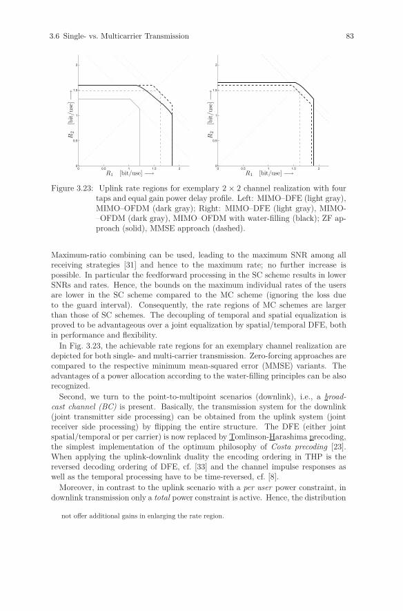
3.6 Single- vs. Multicarrier Transmission 83
0 0.5 1 1.5 20
0.5
1
1.5
2
R1 [bit/use] −→
R2
[bit/use
]−→
0 0.5 1 1.5 20
0.5
1
1.5
2
R1 [bit/use] −→
R2
[bit/use
]−→
Figure 3.23: Uplink rate regions for exemplary 2 × 2 channel realization with fourtaps and equal gain power delay profile. Left: MIMO–DFE (light gray),MIMO–OFDM (dark gray); Right: MIMO–DFE (light gray), MIMO-–OFDM (dark gray), MIMO–OFDM with water-filling (black); ZF ap-proach (solid), MMSE approach (dashed).
Maximum-ratio combining can be used, leading to the maximum SNR among allreceiving strategies [31] and hence to the maximum rate; no further increase ispossible. In particular the feedforward processing in the SC scheme results in lowerSNRs and rates. Hence, the bounds on the maximum individual rates of the usersare lower in the SC scheme compared to the MC scheme (ignoring the loss dueto the guard interval). Consequently, the rate regions of MC schemes are largerthan those of SC schemes. The decoupling of temporal and spatial equalization isproved to be advantageous over a joint equalization by spatial/temporal DFE, bothin performance and flexibility.
In Fig. 3.23, the achievable rate regions for an exemplary channel realization aredepicted for both single- and multi-carrier transmission. Zero-forcing approaches arecompared to the respective minimum mean-squared error (MMSE) variants. Theadvantages of a power allocation according to the water-filling principles can be alsorecognized.
Second, we turn to the point-to-multipoint scenarios (downlink), i.e., a broad-cast channel (BC) is present. Basically, the transmission system for the downlink(joint transmitter side processing) can be obtained from the uplink system (jointreceiver side processing) by flipping the entire structure. The DFE (either jointspatial/temporal or per carrier) is now replaced by Tomlinson-Harashima precoding,the simplest implementation of the optimum philosophy of Costa precoding [23].When applying the uplink-downlink duality the encoding ordering in THP is thereversed decoding ordering of DFE, cf. [33] and the channel impulse responses aswell as the temporal processing have to be time-reversed, cf. [8].
Moreover, in contrast to the uplink scenario with a per user power constraint, indownlink transmission only a total power constraint is active. Hence, the distribution
not offer additional gains in enlarging the rate region.
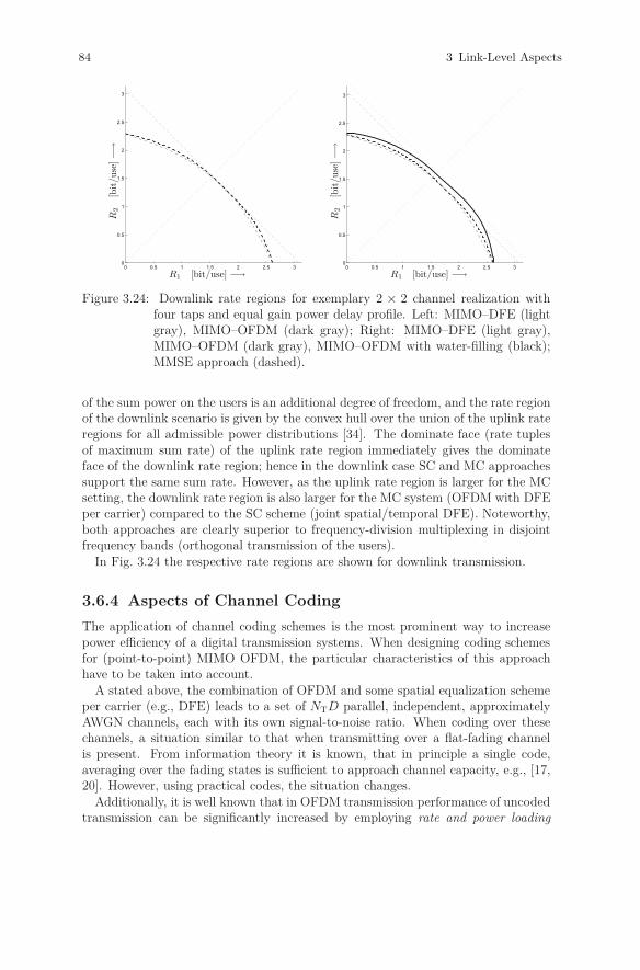
84 3 Link-Level Aspects
0 0.5 1 1.5 2 2.5 30
0.5
1
1.5
2
2.5
3
R1 [bit/use] −→
R2
[bit/use
]−→
0 0.5 1 1.5 2 2.5 30
0.5
1
1.5
2
2.5
3
R1 [bit/use] −→
R2
[bit/use
]−→
Figure 3.24: Downlink rate regions for exemplary 2 × 2 channel realization withfour taps and equal gain power delay profile. Left: MIMO–DFE (lightgray), MIMO–OFDM (dark gray); Right: MIMO–DFE (light gray),MIMO–OFDM (dark gray), MIMO–OFDM with water-filling (black);MMSE approach (dashed).
of the sum power on the users is an additional degree of freedom, and the rate regionof the downlink scenario is given by the convex hull over the union of the uplink rateregions for all admissible power distributions [34]. The dominate face (rate tuplesof maximum sum rate) of the uplink rate region immediately gives the dominateface of the downlink rate region; hence in the downlink case SC and MC approachessupport the same sum rate. However, as the uplink rate region is larger for the MCsetting, the downlink rate region is also larger for the MC system (OFDM with DFEper carrier) compared to the SC scheme (joint spatial/temporal DFE). Noteworthy,both approaches are clearly superior to frequency-division multiplexing in disjointfrequency bands (orthogonal transmission of the users).
In Fig. 3.24 the respective rate regions are shown for downlink transmission.
3.6.4 Aspects of Channel Coding
The application of channel coding schemes is the most prominent way to increasepower efficiency of a digital transmission systems. When designing coding schemesfor (point-to-point) MIMO OFDM, the particular characteristics of this approachhave to be taken into account.
A stated above, the combination of OFDM and some spatial equalization schemeper carrier (e.g., DFE) leads to a set of NTD parallel, independent, approximatelyAWGN channels, each with its own signal-to-noise ratio. When coding over thesechannels, a situation similar to that when transmitting over a flat-fading channelis present. From information theory it is known, that in principle a single code,averaging over the fading states is sufficient to approach channel capacity, e.g., [17,20]. However, using practical codes, the situation changes.
Additionally, it is well known that in OFDM transmission performance of uncodedtransmission can be significantly increased by employing rate and power loading
3.6 Single- vs. Multicarrier Transmission 85
utilizing so-called loading algorithms, e.g., [12,24]. However, loading is based on (atleast partial) channel state information (CSI) at the transmitter and hence is notalways applicable. Moreover, loading and channel coding interact and depend oneach other.
It has been shown [3] that bit-interleaved coded modulation (BICM) [21] is a well-suited solution to improve reliability for highly bandwidth efficient transmission aslong as no rate and power loading is used. Furthermore, large signal constellationsshould be avoided, i.e., the rate of the employed channel code has to be selectedcarefully and taking the required signal constellation for achieving a certain spectralefficiency into account (this holds for BICM in general and is not restricted to MIMOOFDM).
As soon as rate and power loading can be applied, BICM cannot be recommended.Here, the relevant performance measure is the parallel decoding capacity. Unfortu-nately, this quantity cannot be (significantly) improved by loading; some powerloading strategies, well-suited for uncoded transmission, even lead to a decrease incapacity and hence are useless in coded transmission. In contrast to BICM, trellis-coded modulation (TCM) [32]—due to the uncoded bits—does only provide gains incombination with rate and power loading. However, neither conventional BICM norTCM can achieve convincing performance in MIMO OFDM. Uncoded but loadedtransmission offers already good performance a the price of requiring partial TXCSI.
When transmitter-side CSI is available, BICM can be improved by adapting theemployed bit interleaver [9,10]. Taking the actual SNRs of the parallel channels andthe used mapping into consideration, a set of equivalent bit levels can be established;the entire modulation scheme is broken down into its fundamental building blocks.Based on the capacities of these equivalent binary channels, the interleaver is thendesigned such that within the relevant decoding window an optimized (equalized)metric arrangement is present. Such an interleaver design shows gains over both,conventional interleaving and BICM with rate and power loading. Concerning CSI,only the interleaver sequence has to be exchanged between transmitter and receiverand the additional complexity is almost negligible. Moreover, the capacities of theseequivalent binary channels can also be utilized to perform bit-loading in uncodedtransmission very efficiently, see [12, 13]. Finally, a bit-interleaver design for codedmulticarrier transmission using rate and power loading is also possible using the toolof equivalent binary channels [14].
3.6.5 Summary
In summary it can be stated that MIMO OFDM is an attractive transmission schemefor future communication systems. In point-to-point applications, singlecarrier mod-ulation with joint spatial/temporal DFE performs as good as MIMO OFDM withsuited rate and power loading (uncoded transmission; the losses due to the guardinterval and error propagation in the DFE are ignored). Both approaches offerthe same sum rate. The situation changes when multipoint-to-point or point-to-multipoint scenarios are considered. Here, the rate region (which is the relevant as-sessment factor) is always larger for the multicarrier scheme. Moreover, the OFDM
86 3 Link-Level Aspects
scheme inherently offers much more flexibility and adaptivity.However, the advantages of OFDM are paid with the price of increased demands on
the channel coding schemes. Without coding or loading, OFDM exhibits very poorperformance. Rate and power loading requires CSI at the transmitter. Coding overparallel, independent channel with strongly varying quality is also a challenging task;the popular approach of bit-interleaved coded modulation gets worse for very largesignal constellations, which, however, are required in MIMO OFDM. Again, havingtransmitter-side CSI available, using an adapted interleaver, solves the problem ofcoding for MIMO OFDM to a large extent.
Bibliography
Papers Emerged from the Project:
[1] R.F.H. Fischer, C. Stierstorfer, J.B. Huber, “Point-to-Point Transmission overMIMO Channels with Intersymbol Interference: Comparison of Single- andMulticarrier Modulation,” in Proceedings of the 9th International OFDM Work-shop, pp. 1–5, Dresden, Germany, September 2004.
[2] C. Stierstorfer, R.F.H. Fischer, “Comparison of Coding Strategies for Multi-Antenna Multi-Carrier Transmission,” in Proceedings of the 10th InternationalOFDM Workshop, Hamburg, Germany, August/September 2005.
[3] R.F.H. Fischer, C. Stierstorfer, “Comparison of Code Design Requirementsfor Singlecarrier and Multicarrier Transmission over Frequency-Selective MIMOChannels,” in Proceedings IEEE International Symposium on Information The-ory (ISIT 2005), Adelaide, Australia, September 2005.
[4] C. Stierstorfer, R.F.H. Fischer, “Rate Regions for Multipoint-to-Point-Transmission over Channels with Intersymbol Interference,” in Proceedingsof International ITG/IEEE Workshop on Smart Antennas, Castle Reisensburg,Germany, March 2006.
[5] R.F.H. Fischer, C. Stierstorfer, “Single- and Multicarrier Transmission inMultipoint-to-Point Scenarios with Intersymbol Interference: A Comparison,”in Proceedings of 4th International Symposium on Turbo Codes in connectionwith the 6th International ITG-Conference on Source and Channel Coding,München, Germany, April 2006.
[6] C. Stierstorfer, R.F.H. Fischer, “Rate Regions for Multicarrier Point-to-Multipoint Transmission over Channels with Intersymbol Interference,” in Pro-ceedings of the 11th International OFDM Workshop, pp. 293–297, Hamburg,Germany, August 2006.
[7] C. Stierstorfer, R.F.H. Fischer, “(Gray) Mappings for Bit-Interleaved CodedModulation,” in Proceedings of 65th IEEE Vehicular Technology Conference(VTC 2007 Spring), Dublin, Ireland, April 2007.

Bibliography 87
[8] R.F.H. Fischer, C. Stierstorfer, “Single- and Multicarrier Transmission in Up-and Downlink Scenarios with Intersymbol Interference: A Comparison,” Euro-pean Transactions on Telecommunications (ETT), Vol. 18, pp. 467–477, August2007.
[9] C. Stierstorfer, R.F.H. Fischer, “Intralevel Interleaving for BICM in OFDMScenarios,” in Proceedings of 12th International OFDM Workshop, Hamburg,Germany, August 2007.
[10] C. Stierstorfer, R.F.H. Fischer, “Adaptive Interleaving for Bit-InterleavedCoded Modulation,” in Proceedings of 7th International ITG Conference onSource and Channel Coding (SCC), Ulm, Germany, January 2008.
[11] C. Stierstorfer, R.F.H. Fischer, “Mappings for BICM in UWB Scenarios,” inProceedings of 7th International ITG Conference on Source and Channel Coding(SCC), Ulm, Germany, January 2008.
[12] C. Stierstorfer, R.F.H. Fischer, “Rate Loading in OFDM Based on Bit LevelCapacities,” in Proceedings of the International Symposium on InformationTheory (ISIT 2008), Toronto, Canada, July 2008.
[13] C. Stierstorfer, R.F.H. Fischer, “Aspects of Rate and Power Loading in (Coded-)OFDM,” in Proceedings of 13th International OFDM Workshop, Hamburg,Germany, August 2008.
[14] C. Stierstorfer, R.F.H. Fischer, “Asymptotically Optimal Mappings for BICMwith M-PAM and M2-QAM,” IET Electronics Letters, Vol. 45, No. 3, pp. 173–174, January 2009.
[15] C. Stierstorfer, R.F.H. Fischer, “Loading-Aware Bit-Interleaver Design,” in Pro-ceedings of 14th International OFDM Workshop, Hamburg, Germany, Septem-ber 2009.
[16] C. Stierstorfer, A Bit-Level-Based Approach to Coded Multicarrier Transmis-sion,” Dissertation, Univerität Erlangen–Nürnberg, July 2009.
Other References:
[17] E. Biglieri, J. Proakis, S. Shamai (Shitz), “Fading Channels: Information-Theoretic and Communications Aspects,” IEEE Transactions on InformationTheory, pp. 2619–2692. June 1998.
[18] J.A.C. Bingham, “Multicarrier Modulation for Data Transmission: An IdeaWhose Time Has Come,” IEEE Communications Magazine, pp. 5–14, May1990.
[19] H. Boche, M. Schubert, “A General Duality Theory for Uplink and DownlinkBeamforming,” in Proceedings of IEEE Vehicular Technology Conference (VTC2002 Fall), 2002.

88 3 Link-Level Aspects
[20] M. Bossert, A. Donder, V. Zyablov, “OFDM–Übertragung über Mobil-funkkanäle: Bemerkungen zur Kanalkapazität,” in 2. OFDM–Fachgespräch,Braunschweig, Sep. 1997.
[21] G. Caire, G. Taricco, E. Biglieri, “Bit–Interleaved Coded Modulation,” IEEETransactions on Information Theory, pp. 927-–946, May 1998.
[22] J.M. Cioffi, G.P. Dudevoir, M.V. Eyuboglu, G.D. Forney, “MMSE Decision-Feedback Equalizers and Coding — Part I: Equalization Results, Part II:Coding Results,” IEEE Transactions on Communications, pp. 2582–2604,Oct. 1995.
[23] M.H.M. Costa, “Writing on dirty paper,” IEEE Transactions on InformationTheory, pp. 439–441, May 1983.
[24] R.F.H. Fischer, J.B. Huber, “A New Loading Algorithm for Discrete MultitoneTransmission,” in IEEE Global Telecommunications Conference (GLOBECOM’96), London, U.K., pp. 724–728, Nov. 1996.
[25] R.F.H. Fischer, J.B. Huber, “On The Equivalence of Single- and MulticarrierModulation: A New View,” in IEEE International Symposium on InformationTheory (ISIT ’97), p. 197, Ulm, June-July 1997.
[26] R.F.H. Fischer, Precoding and Signal Shaping for Digital Transmission, JohnWiley & Sons, Inc., New York, 2002.
[27] R.F.H. Fischer, J.B. Huber, C. Windpassinger, “Signal Processing inDecision-Feedback Equalization of Intersymbol-Interference and Multiple-Input/ Multiple-Output Channels: A Unified View,” ELSEVIER Signal Processing,Vol. 83, No. 8, pp. 1633–1642, Aug. 2003.
[28] G.J. Foschini, “Layered Space-Time Architecture for Wireless Communicationin a Fading Environment When Using Multiple Antennas,” Bell LaboratoriesTechnical Journal, pp. 41–59, Autumn 1996.
[29] R. Price, “Nonlinear Feedback Equalized PAM versus Capacity for Noisy FilterChannels,” Proc. ICC’72, pp. 22.12–22.17, 1972.
[30] E. Telatar, “Capacity of multi-antenna Gaussian channels,” European Trans-actions on Telecommunications, pp. 585–596, Nov. 1999.
[31] D. Tse, P. Viswanath, Fundamentals of Wireless Communication, CambridgeUniv. Press, Cambridge, UK, 2005.
[32] G. Ungerböck, “Channel Coding with Multilevel/Phase Signals,” IEEE Trans-actions on Information Theory, pp. 55—67, Jan. 1982.
[33] P. Viswanath, D. Tse, “Sum Capacity of the Vector Gaussian Broadcast Chan-nel and Uplink-Downlink Duality,” IEEE Transactions on Information Theory,pp. 1912–1921, Aug. 2003.

Bibliography 89
[34] S. Vishwanath, N. Jindal, A. Goldsmith, “Duality, Achievable Rates, and Sum-Rate Capacity of Gaussian MIMO Broadcast Channels,” IEEE Transactionson Information Theory, pp. 2658–2668, Oct. 2003.
[35] W. Yu, J.M. Cioffi, “Sum Capacity of Gaussian Vector Broadcast Channels,”IEEE Transactions on Information Theory, pp. 1875–1892, Sep. 2004.
[36] N.A. Zervos, I. Kalet, “Optimized Decision Feedback Equalization Versus Opti-mized Orthogonal Frequency Division Multiplexing for High–Speed Data Trans-mission Over the Local Cable Network,” Proc. ICC’89, Boston, pp. 1080–1085,Sep. 1989.
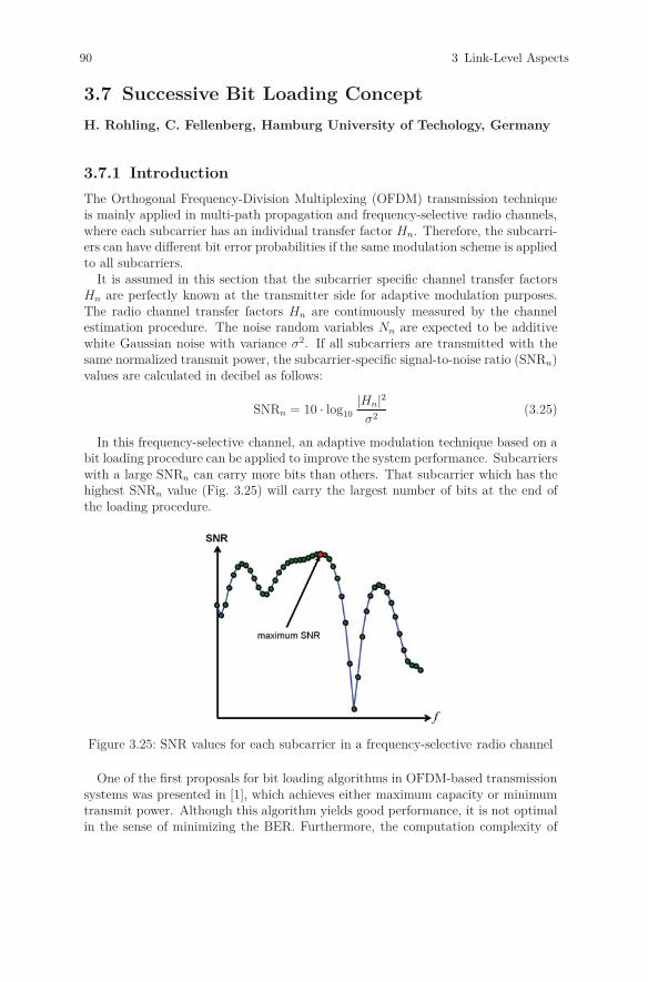
90 3 Link-Level Aspects
3.7 Successive Bit Loading Concept
H. Rohling, C. Fellenberg, Hamburg University of Techology, Germany
3.7.1 Introduction
The Orthogonal Frequency-Division Multiplexing (OFDM) transmission techniqueis mainly applied in multi-path propagation and frequency-selective radio channels,where each subcarrier has an individual transfer factor Hn. Therefore, the subcarri-ers can have different bit error probabilities if the same modulation scheme is appliedto all subcarriers.
It is assumed in this section that the subcarrier specific channel transfer factorsHn are perfectly known at the transmitter side for adaptive modulation purposes.The radio channel transfer factors Hn are continuously measured by the channelestimation procedure. The noise random variables Nn are expected to be additivewhite Gaussian noise with variance σ2. If all subcarriers are transmitted with thesame normalized transmit power, the subcarrier-specific signal-to-noise ratio (SNRn)values are calculated in decibel as follows:
SNRn = 10 · log10
|Hn|2σ2
(3.25)
In this frequency-selective channel, an adaptive modulation technique based on abit loading procedure can be applied to improve the system performance. Subcarrierswith a large SNRn can carry more bits than others. That subcarrier which has thehighest SNRn value (Fig. 3.25) will carry the largest number of bits at the end ofthe loading procedure.
Figure 3.25: SNR values for each subcarrier in a frequency-selective radio channel
One of the first proposals for bit loading algorithms in OFDM-based transmissionsystems was presented in [1], which achieves either maximum capacity or minimumtransmit power. Although this algorithm yields good performance, it is not optimalin the sense of minimizing the BER. Furthermore, the computation complexity of
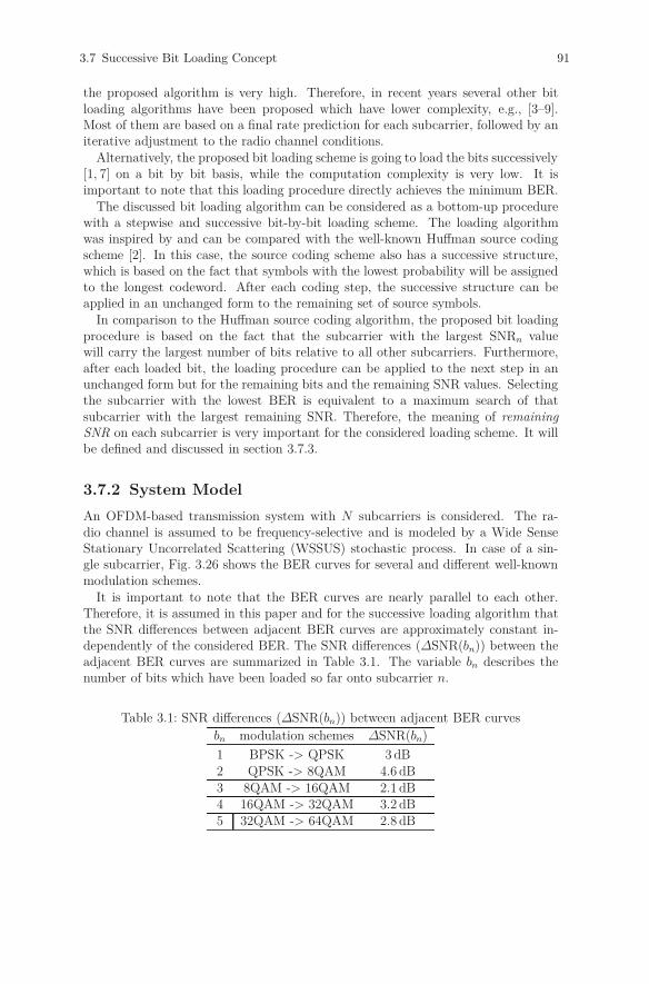
3.7 Successive Bit Loading Concept 91
the proposed algorithm is very high. Therefore, in recent years several other bitloading algorithms have been proposed which have lower complexity, e.g., [3–9].Most of them are based on a final rate prediction for each subcarrier, followed by aniterative adjustment to the radio channel conditions.
Alternatively, the proposed bit loading scheme is going to load the bits successively[1, 7] on a bit by bit basis, while the computation complexity is very low. It isimportant to note that this loading procedure directly achieves the minimum BER.
The discussed bit loading algorithm can be considered as a bottom-up procedurewith a stepwise and successive bit-by-bit loading scheme. The loading algorithmwas inspired by and can be compared with the well-known Huffman source codingscheme [2]. In this case, the source coding scheme also has a successive structure,which is based on the fact that symbols with the lowest probability will be assignedto the longest codeword. After each coding step, the successive structure can beapplied in an unchanged form to the remaining set of source symbols.
In comparison to the Huffman source coding algorithm, the proposed bit loadingprocedure is based on the fact that the subcarrier with the largest SNRn valuewill carry the largest number of bits relative to all other subcarriers. Furthermore,after each loaded bit, the loading procedure can be applied to the next step in anunchanged form but for the remaining bits and the remaining SNR values. Selectingthe subcarrier with the lowest BER is equivalent to a maximum search of thatsubcarrier with the largest remaining SNR. Therefore, the meaning of remainingSNR on each subcarrier is very important for the considered loading scheme. It willbe defined and discussed in section 3.7.3.
3.7.2 System Model
An OFDM-based transmission system with N subcarriers is considered. The ra-dio channel is assumed to be frequency-selective and is modeled by a Wide SenseStationary Uncorrelated Scattering (WSSUS) stochastic process. In case of a sin-gle subcarrier, Fig. 3.26 shows the BER curves for several and different well-knownmodulation schemes.
It is important to note that the BER curves are nearly parallel to each other.Therefore, it is assumed in this paper and for the successive loading algorithm thatthe SNR differences between adjacent BER curves are approximately constant in-dependently of the considered BER. The SNR differences (ΔSNR(bn)) between theadjacent BER curves are summarized in Table 3.1. The variable bn describes thenumber of bits which have been loaded so far onto subcarrier n.
Table 3.1: SNR differences (ΔSNR(bn)) between adjacent BER curvesbn modulation schemes ΔSNR(bn)
1 BPSK -> QPSK 3 dB2 QPSK -> 8QAM 4.6 dB3 8QAM -> 16QAM 2.1 dB4 16QAM -> 32QAM 3.2 dB5 32QAM -> 64QAM 2.8 dB
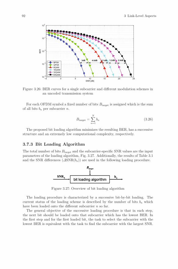
92 3 Link-Level Aspects
−5 0 5 10 15 20 2510−4
10−3
10−2
10−1
100
SNR [dB]
BE
R
BPSKQPSK8QAM16QAM32QAM64QAM
3dB 2.8dB2.1dB 3.2dB4.6dB
Figure 3.26: BER curves for a single subcarrier and different modulation schemes inan uncoded transmission system
For each OFDM symbol a fixed number of bits Btarget is assigned which is the sumof all bits bn per subcarrier n.
Btarget =N∑
n=1
bn (3.26)
The proposed bit loading algorithm minimizes the resulting BER, has a successivestructure and an extremely low computational complexity, respectively.
3.7.3 Bit Loading Algorithm
The total number of bits Btarget and the subcarrier-specific SNR values are the inputparameters of the loading algorithm, Fig. 3.27. Additionally, the results of Table 3.1and the SNR differences (ΔSNR(bn)) are used in the following loading procedure.
bit loading algorithmn
SNRn
b
targetB
bit loading algorithmn
SNRn
b
targetB
Figure 3.27: Overview of bit loading algorithm
The loading procedure is characterized by a successive bit-by-bit loading. Thecurrent status of the loading scheme is described by the number of bits bn whichhave been loaded onto the different subcarrier n so far.
The general objective of the successive loading procedure is that in each step,the next bit should be loaded onto that subcarrier which has the lowest BER. Inthe first step and for the first loaded bit, the task to select the subcarrier with thelowest BER is equivalent with the task to find the subcarrier with the largest SNR.
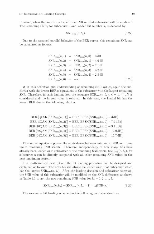
3.7 Successive Bit Loading Concept 93
However, when the first bit is loaded, the SNR on that subcarrier will be modified.The remaining SNRn for subcarrier n and loaded bit number bn is denoted by
SNRrem(n, bn). (3.27)
Due to the assumed parallel behavior of the BER curves, this remaining SNR canbe calculated as follows:
SNRrem(n, 1) = SNRrem(n, 0) − 3 dB
SNRrem(n, 2) = SNRrem(n, 1) − 4.6 dB
SNRrem(n, 3) = SNRrem(n, 2) − 2.1 dB
SNRrem(n, 4) = SNRrem(n, 3) − 3.2 dB
SNRrem(n, 5) = SNRrem(n, 4) − 2.8 dB
SNRrem(n, 6) = −∞ (3.28)
With this definition and understanding of remaining SNR values, again the sub-carrier with the lowest BER is equivalent to the subcarrier with the largest remainingSNR. Therefore, in each loading step the sequence SNRrem(n, bn), n = 1, · · · , N isconsidered and the largest value is selected. In this case, the loaded bit has thelowest BER due to the following relation:
BER [QPSK(SNRrem(n, 1))] = BER [BPSK(SNRrem(n, 0) − 3 dB]
BER [8QAM(SNRrem(n, 2))] = BER [BPSK(SNRrem(n, 0) − 7.6 dB)]
BER [16QAM(SNRrem(n, 3))] = BER [BPSK(SNRrem(n, 0) − 9.7 dB)]
BER [32QAM(SNRrem(n, 4))] = BER [BPSK(SNRrem(n, 0) − 12.9 dB)]
BER [64QAM(SNRrem(n, 5))] = BER [BPSK(SNRrem(n, 0) − 15.7 dB)]
This set of equations proves the equivalence between minimum BER and max-imum remaining SNR search. Therefore, independently of how many bits havealready been loaded onto subcarrier n, the remaining SNR value, SNRrem(n, bn), forsubcarrier n can be directly compared with all other remaining SNR values in thenext maximum search.
In a mathematical description, the bit loading procedure can be designed andexplained as follows: The next bit will always be loaded onto that subcarrier whichhas the largest SNRrem(n, bn). After the loading decision and subcarrier selection,the SNR value of this subcarrier will be modified by the SNR differences as shownin Table 3.1 to get the new remaining SNR value for bn = 1, 2, . . . , 5.
SNRrem(n, bn) = SNRrem(n, bn − 1) − ΔSNR(bn) (3.29)
The successive bit loading scheme has the following recursive structure:
94 3 Link-Level Aspects
1. Initialize bn = 0 and SNRrem(n, 0) = SNRn for all n = 1, . . . , N
2. Select that subcarrier which has the largest remaining SNR valueSNRrem(i, bi)
3. Load the next bit onto the selected subcarrier with index i: bi = bi +1
4. Calculate the remaining SNR value SNRrem(i, bi)
SNRrem(i, bi) = SNRrem(i, bi − 1) −
⎧⎪⎪⎪⎪⎪⎪⎨⎪⎪⎪⎪⎪⎪⎩
3.0 dB, if bi = 1
4.6 dB, if bi = 2
2.1 dB, if bi = 3
3.2 dB, if bi = 4
2.8 dB, if bi = 5
5. Repeat step 2 to 4 until∑
bn = Btarget
This loading scheme has a pure bottom-up and successive structure. The BER isminimized and the bit loading procedure results in the number of bits bn loaded ontosubcarrier n. The transmit power is assumed to be identical for each subcarrier.
3.7.4 Results
An OFDM-based transmission system with N = 256 subcarriers is considered. Theradio channel is assumed to be frequency-selective and will be simulated by a WSSUSmodel. Three different loading algorithms are analyzed and compared with a non-adaptive modulation procedure. In addition to the proposed loading algorithm, thealgorithm described in [3] (maximum capacity) and the algorithm described in [4](minimum SER) are considered in the simulation.
The resulting BER performance for this bit loading algorithm and for a bandwidthefficiency of 2 bit/s/Hz in an uncoded system is shown in Fig. 3.28. The transmitpower is assumed to be uniformly distributed over all loaded subcarriers.
In comparison to the non-adaptive modulation scheme, all adaptive bit loadingalgorithms achieve tremendous gains. The proposed bit loading procedure has anadvantage of 0.2 dB in SNR compared with the loading scheme described in [4].The resulting computation complexity of this new bit loading procedure is very lowsince only the calculation of SNR differences and some sorting procedures have tobe performed.
Although the described bit loading procedure is optimum in the sense of minimumBER, the subcarriers will have different bit error probabilities at the end of the load-ing procedure due to the subcarrier-specific remaining SNR values, SNRrem(n, bn−1).
BERn = BER[BPSK(SNRrem(n, bn − 1))] (3.30)
However, the proposed bit loading algorithm can be extended by an additionalpower loading scheme. The objective of the power loading scheme is to have thesame BER on all subcarriers.

3.7 Successive Bit Loading Concept 95
5 6 7 8 9 10 11 12 13 14 1510−4
10−3
10−2
10−1
100
SNR [dB]
BE
R
non−adaptive modulationmaximum capacity [3]minimum SER [4]proposed scheme
Figure 3.28: BER performance curves for different bit loading schemes in an uncodedsystem; bandwidth efficiency = 2 bit/s/Hz
The subcarrier-specific remaining SNR values, SNRrem(n, bn − 1), are consideredfor the additional power loading procedure. First, the maximum remaining SNR iscalculated.
SNRrem,max = maxi
(SNRrem(i, bi − 1)
)(3.31)
The transmit power of each subcarrier is boosted by a scaling factor an until allsubcarriers have the same BER. The scaling factor an in decibel is determined asfollows:
an = SNRrem,max − SNRrem(n, bn − 1). (3.32)
This power loading procedure is illustrated in Fig. 3.29 and 3.30 as an examplewith 10 subcarriers, different remaining SNRrem(n, bn −1) values, and resulting BERfigures, respectively.
1 2 3 4 5 6 7 8 9 106
7
8
9
subcarriers
SN
Rre
m
2 4 6 8 1010−5
10−4
10−3
10−2
subcarriers
BE
R
Figure 3.29: Remaining SNRrem(n, bn −1) and resulting BER for a uniform transmitpower distribution
Figure 3.29 shows the resulting BER for each subcarrier if a uniform transmitpower is assumed. The BER can be directly calculated by the subcarrier-specificremaining SNR value.

96 3 Link-Level Aspects
After the bit loading procedure, the transmit power is boosted by the scalingfactor an to get the same BER for each subcarrier. The resulting BER values areshown in Fig. 3.30.
1 2 3 4 5 6 7 8 9 106
7
8
9
subcarriers
SN
Rre
m
2 4 6 8 10
10−4
10−3
10−2
subcarriers
BE
R
10−5
Figure 3.30: Subcarrier specific SNRrem(n, bn − 1) with power loading based on thescaling factor an procedure
In Fig. 3.31, the results of a joint bit and power loading scheme are depicted. Aclear difference in BER performance between the loading algorithms for a bandwidthefficiency of 2 bit/s/Hz can be observed. The proposed loading procedure has a0.3 dB better performance compared to the loading scheme described in [4].
5 6 7 8 9 10 11 12 13 14 1510−4
10−3
10−2
10−1
100
SNR [dB]
BE
R
non−adaptive modulationmaximum capacity [3]minimum SER [4]proposed scheme
Figure 3.31: BER performance curves for the joint bit and power loading algorithmsin an uncoded system, bandwidth efficiency = 2 bit/s/Hz
3.7.5 Summary
A new successive bit loading algorithm has been proposed which directly minimizesthe resulting BER. Furthermore, this scheme has a very low computational com-plexity. An important point is the calculation of the remaining SNR. Independentlyof how many bits have been already loaded onto the different subcarriers, the values
3.7 Successive Bit Loading Concept 97
of remaining SNR can be directly compared with each other and can be used for amaximum search.
Therefore, it is possible to assign the next bit to that subcarrier which has thelargest remaining SNR. In this case, the resulting BER is minimized and the pro-posed loading algorithm shows a difference of 0.2 dB in the BER performance com-pared with [4]. This is a small difference in system performance, but the computa-tional complexity of this loading scheme is very low. In each step of the bit loadingprocedure, a single difference must be calculated and a maximum search is necessary.
This bit loading scheme can be extended by an additional power loading proce-dure based on the introduced logarithmic scaling factor an. In this way, the BERperformance is improved by 0.3 dB.
Bibliography
[1] D. Hughes-Hartogs, “Ensemble modem structure for imperfect transmissionmedia”, United States Patent no. 4,833,796, May 1989
[2] D. A. Huffman, “A method for the construction of minimum-redundancycodes”, Proceedings IRE, pp. 1098-1101, September 1952
[3] P. S. Chow, J. M. Cioffi and J. A. C. Bingham, “A Practical Discrete MultitoneTransceiver Loading Algorithm for Data Transmission over Spectrally ShapedChannels”, IEEE Transactions on Communications, vol. 43, no. 2/3/4, pp.773-775, Feb./Mar./Apr., 1995
[4] R. F. H. Fischer and J. B. Huber, “A New Loading Algorithm for Discrete Multi-tone Transmission”, Proceedings of Global Telecommunications Conference, pp.724-728, London, UK, Novemeber 1996
[5] J. Campello, “Practical Bit Loading for DMT”, IEEE International Conferenceon Communications, pp. 801-805, Vancouver, Canada, 1999
[6] W. Henkel and K. Hassan, “OFDM (DMT) Bit and Power Loading for UnequalError Protection”, 11th International OFDM-Workshop, pp. 36-40, Hamburg,Germany, 2006
[7] D. A. Bui, C. Fellenberg, H. Rohling, “Successive bit loading scheme with lowcomputation complexity”, 13th International OFDM-Workshop, pp. 115-118,Hamburg, Germany, 2008
[8] H. E. Levin, “A Complete and Optimal Data Allocation Method for PracticalDiscrete Multitone Systems”, Global Telecommunications Conference 2001, pp.369-374, San Antonio, USA, 2001
[9] R. Grünheid, E. Bolinth and H. Rohling, “A Blockwise Loading Algorithm forthe Adaptive Modulation Technique in OFDM Systems”, Proc. IEEE VTC Fall2001, Atlantic City, October 2001
98 3 Link-Level Aspects
3.8 Adaptive Transmission Techniques
A. Czylwik, University of Duisburg-Essen, Germany
3.8.1 Introduction
The concept of adaptive modulation and coding is very well established for twistedpair communications. The corresponding method is discrete multitone transmission,see, e.g., [1]. In DMT, different modulation schemes with different bandwidth ef-ficiencies are used in order to most efficiently transmit via the frequency-selectivetwisted pair channel. The process of distribution of information on the differentsubcarriers is called bit-loading, where the optimum bitloading method is describedin [2]. The information bits are distributed in a way that the bit error probabilitiesare as small as possible and almost equal for each subcarrier.
In principle, this concept can also be applied for transmission via multipath radiochannels. Besides the aspect that DMT transmission is a baseband concept, the onlyfundamental difference is the time variance of the radio channel. Therefore, it hasbeen proposed to use adaptive modulation techniques also for radio communications[3].
Because of small-scale fading, the capacity of time-variant radio channels variesalso with time. For strong multipath propagation it can be assumed that eachsubcarrier shows approximately Rayleigh fading statistics. The correlation betweenfading of subchannels decreases with increasing frequency separation. Thus, for abroadband channel these fluctuations cancel out partly so that the fluctuations ofthe overall broadband channel are reduced. It has been shown in [4], [5] that theremaining fluctuations of the channel capacity depend on the relation between avail-able bandwidth and coherence bandwidth of the channel. For a system bandwidthsignificantly larger than the coherence bandwidth of the channel, the remainingfluctuations are proportional to the square root of the system bandwidth.
In case of time-variant channels with corresponding time-variant capacity, twodifferent adaptation concepts can be applied. One possibility is to keep the trans-mission quality (bit error probability) constant and let the data rate fluctuate. Theother possibility is to keep the data rate constant and let the transmission qualityfluctuate. Since most transmission services require a piecewise constant data ratecorresponding to a given transmission frame, only the case of constant data rate andfluctuating bit error probability is considered in the following. An overview aboutadaptive multicarrier modulation can be found in [6].
3.8.2 Adaptive Modulation and Coding
For single input single output (SISO) systems, by adaptive modulation a substantialgain compared with fixed modulation can be obtained. Simulation results showthat performance gains of up to 12 dB can be achieved. If adaptive modulation isutilized, additional adaptive coding does not yield significant improvements, since byadaptive modulation the bit error probabilities for all subcarriers are approximately
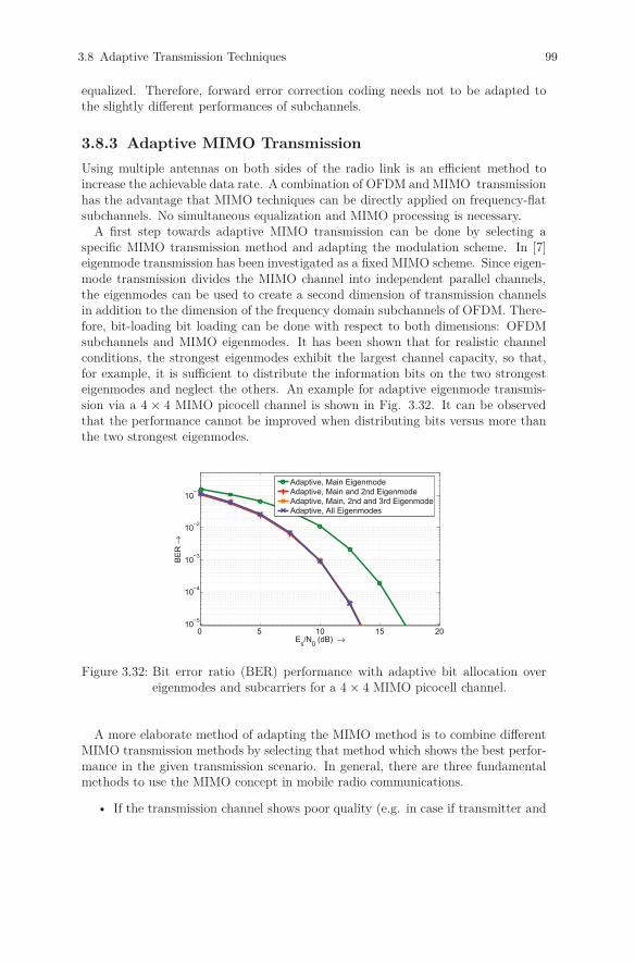
3.8 Adaptive Transmission Techniques 99
equalized. Therefore, forward error correction coding needs not to be adapted tothe slightly different performances of subchannels.
3.8.3 Adaptive MIMO Transmission
Using multiple antennas on both sides of the radio link is an efficient method toincrease the achievable data rate. A combination of OFDM and MIMO transmissionhas the advantage that MIMO techniques can be directly applied on frequency-flatsubchannels. No simultaneous equalization and MIMO processing is necessary.
A first step towards adaptive MIMO transmission can be done by selecting aspecific MIMO transmission method and adapting the modulation scheme. In [7]eigenmode transmission has been investigated as a fixed MIMO scheme. Since eigen-mode transmission divides the MIMO channel into independent parallel channels,the eigenmodes can be used to create a second dimension of transmission channelsin addition to the dimension of the frequency domain subchannels of OFDM. There-fore, bit-loading bit loading can be done with respect to both dimensions: OFDMsubchannels and MIMO eigenmodes. It has been shown that for realistic channelconditions, the strongest eigenmodes exhibit the largest channel capacity, so that,for example, it is sufficient to distribute the information bits on the two strongesteigenmodes and neglect the others. An example for adaptive eigenmode transmis-sion via a 4 × 4 MIMO picocell channel is shown in Fig. 3.32. It can be observedthat the performance cannot be improved when distributing bits versus more thanthe two strongest eigenmodes.
0 5 10 15 2010−5
10−4
10−3
10−2
10−1
Es/N0 (dB) →
BE
R →
Adaptive, Main EigenmodeAdaptive, Main and 2nd EigenmodeAdaptive, Main, 2nd and 3rd EigenmodeAdaptive, All Eigenmodes
Figure 3.32: Bit error ratio (BER) performance with adaptive bit allocation overeigenmodes and subcarriers for a 4 × 4 MIMO picocell channel.
A more elaborate method of adapting the MIMO method is to combine differentMIMO transmission methods by selecting that method which shows the best perfor-mance in the given transmission scenario. In general, there are three fundamentalmethods to use the MIMO concept in mobile radio communications.
• If the transmission channel shows poor quality (e.g. in case if transmitter and
100 3 Link-Level Aspects
receiver are far away from each other), diversity concepts can be used to reduceerror probabilities while transmitting with small data rates.
• If the channel is in good condition (including sufficient scattering), spatialmultiplexing may be used to increase data rates.
• Finally, if the channel is in a quite good condition, but there is severe co-channel interference, multiple antennas may be used for beamforming in orderto suppress the interference.
A criterion has to be elaborated which tells the system when to switch betweenthe different MIMO transmission modes. A simple and very practical method forchoosing the MIMO method is the exponential effective SNR mapping (EESM) ap-proach [8] which has been originally developed for non-adaptive SISO-OFDM trans-mission. The EESM approach maps the N subcarrier SNRs γk at the receiver incase of a frequency-selective channel to an effective SNR γeff :
γeff = −β ln
(1
N
N∑k=1
e−γkβ
)(3.33)
The effective SNR γeff is calculated in such a way that the bit error ratio (BER)of the OFDM system with the frequency-selective channel equals the BER of afrequency-flat AWGN channel with the SNR γeff . Therefore, the EESM methodmaps the performance of a frequency-selective channel to single value which is usedas an interface between link and system level simulations. The EESM method canbe extended to adaptively bit-loaded OFDM transmission systems with convolu-tional coding and soft decision decoding [9]. Furthermore, it can also be efficientlyadapted to different MIMO schemes: In [10] the EESM approach is extended tospace-frequency coding as well as spatial multiplexing.
The performance of adaptive MIMO transmission with bit interleaved convolu-tionally coded modulation has been analyzed in [11] and [12]. In Figs. 3.33 and 3.34different adaptive 2 × 2 MIMO-OFDM techniques are compared with the averagenormalized channel capacity C/B:
• Spatial multiplexing (SM) with VBLAST detection and per antenna rate con-trol (PARC) and fixed modulation on all subcarriers.
• Transmit diversity realized by rate 1 space-frequency coding (SFC) with fixedmodulation on all subcarriers.
• Adaptive MIMO transmission (switching between SM and SFC) with fixedmodulation on all subcarriers.
• Adaptive MIMO transmission (switching between SM and SFC) with opti-mized bit-loading.
The MIMO schemes are adapted for each OFDM block (symbol) - this means thatfor all subcarriers the same MIMO scheme is used. Obviously, for a multipath-richchannel and high SNR values (see Fig. 3.33) spatial multiplexing results in a higher

3.8 Adaptive Transmission Techniques 101
information rate. In case of a channel with a small amount of propagation paths andlarge spatial correlation, space-frequency coding clearly outperforms spatial multi-plexing. Adaptive MIMO transmission shows a performance at least as good as SMor SFC. It can be observed that – independent of the channel – bit-loading resultsin an additional performance gain.
10 lg ES/N0 (dB) →
Info
rmat
ion
bit
s/
sub
chan
nel
use
→
SM with VBLAST and PARCDiversity by SFCAdaptive MIMOBit-loaded adaptive MIMOC/B
-5 0 5 10 15 20 25 30 350
2
4
6
8
10
12
Figure 3.33: Comparison of adaptive MIMO transmission methods with fixed MIMOtransmission. [12]. Channel type I: multipath-rich MIMO channel withlow spatial correlation.
10 lg ES/N0 (dB) →
Info
rmat
ion
bit
s/
sub
chan
nel
use
→
SM with VBLAST and PARCDiversity by SFCAdaptive MIMOBit-loaded adaptive MIMOC/B
-5 0 5 10 15 20 25 30 350
2
4
6
8
10
12
Figure 3.34: Comparison of adaptive MIMO transmission methods with fixed MIMOtransmission. [12]. Channel type II: MIMO channel with a smallamount of multipath contributions and large spatial correlation.
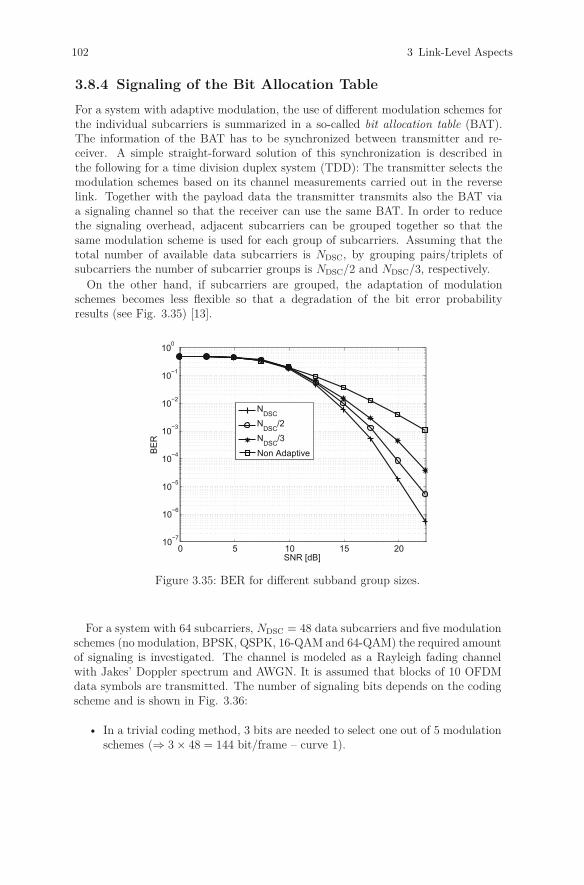
102 3 Link-Level Aspects
3.8.4 Signaling of the Bit Allocation Table
For a system with adaptive modulation, the use of different modulation schemes forthe individual subcarriers is summarized in a so-called bit allocation table (BAT).The information of the BAT has to be synchronized between transmitter and re-ceiver. A simple straight-forward solution of this synchronization is described inthe following for a time division duplex system (TDD): The transmitter selects themodulation schemes based on its channel measurements carried out in the reverselink. Together with the payload data the transmitter transmits also the BAT viaa signaling channel so that the receiver can use the same BAT. In order to reducethe signaling overhead, adjacent subcarriers can be grouped together so that thesame modulation scheme is used for each group of subcarriers. Assuming that thetotal number of available data subcarriers is NDSC, by grouping pairs/triplets ofsubcarriers the number of subcarrier groups is NDSC/2 and NDSC/3, respectively.
On the other hand, if subcarriers are grouped, the adaptation of modulationschemes becomes less flexible so that a degradation of the bit error probabilityresults (see Fig. 3.35) [13].
0 5 10 15 2010−7
10−6
10−5
10−4
10−3
10−2
10−1
100
SNR [dB]
BE
R
NDSCN
DSC/2
NDSC/3
Non Adaptive
Figure 3.35: BER for different subband group sizes.
For a system with 64 subcarriers, NDSC = 48 data subcarriers and five modulationschemes (no modulation, BPSK, QSPK, 16-QAM and 64-QAM) the required amountof signaling is investigated. The channel is modeled as a Rayleigh fading channelwith Jakes’ Doppler spectrum and AWGN. It is assumed that blocks of 10 OFDMdata symbols are transmitted. The number of signaling bits depends on the codingscheme and is shown in Fig. 3.36:
• In a trivial coding method, 3 bits are needed to select one out of 5 modulationschemes (⇒ 3 × 48 = 144 bit/frame – curve 1).
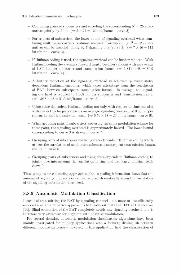
3.8 Adaptive Transmission Techniques 103
• Combining pairs of subcarriers and encoding the corresponding 52 = 25 alter-natives jointly by 5 bits (⇒ 5 × 24 = 120 bit/frame – curve 2).
• For triplets of subcarriers, the lower bound of signaling overhead when com-bining multiple subcarriers is almost reached: Corresponding 53 = 125 alter-natives can be encoded jointly by 7 signaling bits (curve 3). (⇒ 7 × 16 = 112bit/frame – curve 3).
• If Huffman coding is used, the signaling overhead can be further reduced. WithHuffman coding the average codeword length becomes random with an averageof 1.811 bit per subcarrier and transmission frame. (⇒ 1.811 × 48 = 86.9bit/frame – curve 4).
• A further reduction of the signaling overhead is achieved by using state-dependent Huffman encoding, which takes advantage from the correlationof BATs between subsequent transmission frames. In average, the signal-ing overhead is reduced to 1.068 bit per subcarrier and transmission frame.(⇒ 1.068 × 48 = 51.3 bit/frame – curve 5).
• Using state-dependent Huffman coding not only with respect to time but alsowith respect to frequency yields an average signaling overhead of 0.56 bit persubcarrier and transmission frame. (⇒ 0.56 × 48 = 26.9 bit/frame – curve 6).
• When grouping pairs of subcarriers and using the same modulation scheme forthese pairs, the signaling overhead is approximately halved. The lower boundcorresponding to curve 3 is shown in curve 7.
• Grouping pairs of subcarriers and using state-dependent Huffman coding whichutilizes the correlation of modulation schemes in subsequent transmission frames,results in curve 8.
• Grouping pairs of subcarriers and using state-dependent Huffman coding tojointly take into account the correlation in time and frequency domain, yieldscurve 9.
These simple source encoding approaches of the signaling information shows that theamount of signaling information can be reduced dramatically when the correlationof the signaling information is utilized.
3.8.5 Automatic Modulation Classification
Instead of transmitting the BAT by signaling channels in a more or less efficientlyencoded way, an alternative approach is to blindly estimate the BAT at the receiver[14]. Blind estimation of the BAT completely avoids any signaling overhead and istherefore very attractive for a system with adaptive modulation.
For several decades, automatic modulation classification algorithms have beenmainly investigated for military applications with a focus to distinguish betweendifferent modulation types – however, in this application field the classification of
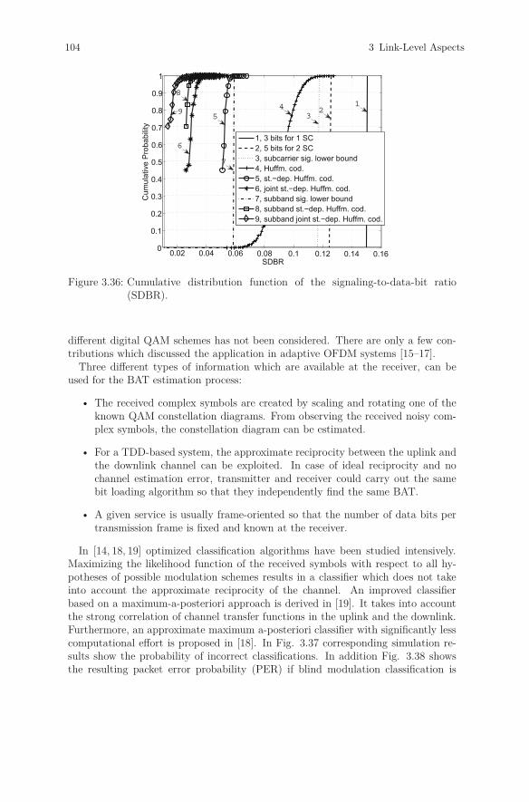
104 3 Link-Level Aspects
0.02 0.04 0.06 0.08 0.1 0.12 0.14 0.160
0.1
0.2
0.3
0.4
0.5
0.6
0.7
0.8
0.9
1
SDBR
Cum
ulat
ive
Pro
babi
lity
1, 3 bits for 1 SC2, 5 bits for 2 SC3, subcarrier sig. lower bound4, Huffm. cod.5, st.−dep. Huffm. cod.6, joint st.−dep. Huffm. cod.7, subband sig. lower bound8, subband st.−dep. Huffm. cod.9, subband joint st.−dep. Huffm. cod.
9
6
8
5
7
43
21
Figure 3.36: Cumulative distribution function of the signaling-to-data-bit ratio(SDBR).
different digital QAM schemes has not been considered. There are only a few con-tributions which discussed the application in adaptive OFDM systems [15–17].
Three different types of information which are available at the receiver, can beused for the BAT estimation process:
• The received complex symbols are created by scaling and rotating one of theknown QAM constellation diagrams. From observing the received noisy com-plex symbols, the constellation diagram can be estimated.
• For a TDD-based system, the approximate reciprocity between the uplink andthe downlink channel can be exploited. In case of ideal reciprocity and nochannel estimation error, transmitter and receiver could carry out the samebit loading algorithm so that they independently find the same BAT.
• A given service is usually frame-oriented so that the number of data bits pertransmission frame is fixed and known at the receiver.
In [14, 18, 19] optimized classification algorithms have been studied intensively.Maximizing the likelihood function of the received symbols with respect to all hy-potheses of possible modulation schemes results in a classifier which does not takeinto account the approximate reciprocity of the channel. An improved classifierbased on a maximum-a-posteriori approach is derived in [19]. It takes into accountthe strong correlation of channel transfer functions in the uplink and the downlink.Furthermore, an approximate maximum a-posteriori classifier with significantly lesscomputational effort is proposed in [18]. In Fig. 3.37 corresponding simulation re-sults show the probability of incorrect classifications. In addition Fig. 3.38 showsthe resulting packet error probability (PER) if blind modulation classification is

3.8 Adaptive Transmission Techniques 105
used. Obviously, using the approximate maximum-a-posteriori (AMAP) approachshows only a small degradation compared with adaptive modulation and perfectBAT knowledge. If the length of the transmission frame is larger, a further reduceddegradation can be observed.
5 10 15 20 2510−3
10−2
10−1
100
SNR [dB]
Prob
abili
ty o
f inc
orre
ct c
lass
ifica
tions
MLMAPAMAP, w=0.8
Figure 3.37: Probability of incorrect classifications of the BAT for different auto-matic modulation classification algorithms: ML = maximum likeli-hood approach, MAP = maximum-a-posteriori approach, AMAP =approximated maximum-a-posteriori approach. Parameters: FFT sizeN = 64, guard interval Ng = 16, bandwidth B = 20 MHz, band-width efficiencies: 0, 1, 2, 4, 6 bit/symbol, average bandwidth effi-ciency: 4 bit/symbol, pairs of subcarriers are grouped, frame length:K = 10 OFDM symbols ⇒ modulation classifications are based on20 received symbols, channel model: IEEE 802.11a indoor with delayspread τds = 100 ns and Doppler frequency fdop = 10 Hz.
3.8.6 Summary
The capacity of an OFDM mobile radio link can be significantly increased usingadaptive transmission techniques. For SISO systems, adaptive modulation can beutilized in order to adapt the transmission scheme to the radio channel as good aspossible. In case of systems with multiple antennas, in addition to the modulationscheme also the MIMO scheme can be adapted to the radio channel.
The main drawback of adaptive modulation is that requires synchronization be-tween transmitter and receiver with respect to the modulation scheme. If signalingis used for synchronization, the amount of signaling can be significantly reduced byusing simple source coding concepts. As a very interesting alternative, synchroniza-tion can be realized by blind estimation of modulation schemes at the receiver, sothat no signaling at all is necessary.
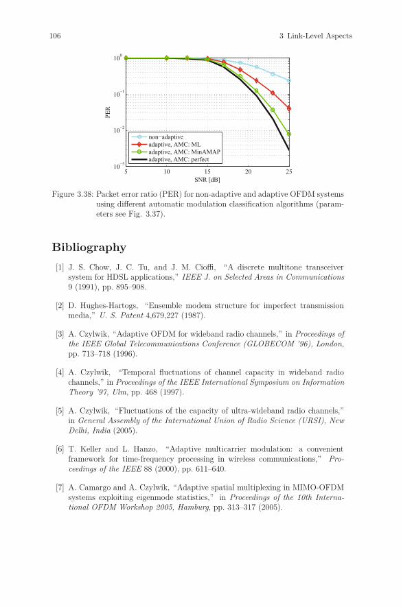
106 3 Link-Level Aspects
5 10 15 20 2510−3
10−2
10−1
100
SNR [dB]
PER
non−adaptiveadaptive, AMC: MLadaptive, AMC: MinAMAPadaptive, AMC: perfect
Figure 3.38: Packet error ratio (PER) for non-adaptive and adaptive OFDM systemsusing different automatic modulation classification algorithms (param-eters see Fig. 3.37).
Bibliography
[1] J. S. Chow, J. C. Tu, and J. M. Cioffi, “A discrete multitone transceiversystem for HDSL applications,” IEEE J. on Selected Areas in Communications9 (1991), pp. 895–908.
[2] D. Hughes-Hartogs, “Ensemble modem structure for imperfect transmissionmedia,” U. S. Patent 4,679,227 (1987).
[3] A. Czylwik, “Adaptive OFDM for wideband radio channels,” in Proceedings ofthe IEEE Global Telecommunications Conference (GLOBECOM ’96), London,pp. 713–718 (1996).
[4] A. Czylwik, “Temporal fluctuations of channel capacity in wideband radiochannels,” in Proceedings of the IEEE International Symposium on InformationTheory ’97, Ulm, pp. 468 (1997).
[5] A. Czylwik, “Fluctuations of the capacity of ultra-wideband radio channels,”in General Assembly of the International Union of Radio Science (URSI), NewDelhi, India (2005).
[6] T. Keller and L. Hanzo, “Adaptive multicarrier modulation: a convenientframework for time-frequency processing in wireless communications,” Pro-ceedings of the IEEE 88 (2000), pp. 611–640.
[7] A. Camargo and A. Czylwik, “Adaptive spatial multiplexing in MIMO-OFDMsystems exploiting eigenmode statistics,” in Proceedings of the 10th Interna-tional OFDM Workshop 2005, Hamburg, pp. 313–317 (2005).

Bibliography 107
[8] Ericsson, System-level evaluation of OFDM – further considerations. 3GPPTSG-RAN WG 1 35, R1-031303, Nov. 17-21, 2003.
[9] A. Camargo and A. Czylwik, “PER prediction for bit-loaded BICM-OFDMwith hard decision Viterbi decoding,” in Proceedings of the 11th InternationalOFDM Workshop 2006, Hamburg, pp. 26–30 (2006).
[10] A. Camargo, D. Yao, P. Paunov, and A. Czylwik, “Adaptive MIMO scheme forBICM OFDM by link adaptation and per-antenna rate control,” in Proceedingsof the 12th International OFDM Workshop 2007, Hamburg, pp. 286–290 (2007).
[11] A. Camargo, D. Yao, and A. Czylwik, “Bandwidth efficiency of practicalMIMO-OFDM systems with adaptive MIMO schemes,” in Proceedings ofthe IEEE International Communications Conference (ICC’09), Dresden (June2009).
[12] A. Camargo, Adaptive modulation, channel coding and MIMO schemes for prac-tical OFDM systems (PhD thesis at the University Duisburg-Essen). Shaker-Verlag, Aachen 2009.
[13] Y. Chen, L. Häring, and A. Czylwik, “Reduction of AM-induced signallingoverhead in WLAN-based OFDM systems statistics,” in Proceedings of the14th International OFDM Workshop 2009, Hamburg (2009).
[14] L. Häring, A. Czylwik, and Y. Chen, “Automatic modulation classificationin application to wireless OFDM systems with adaptive modulation in TDDmode,” In Proceedings of the 13th International OFDM Workshop 2008, Ham-burg (Aug. 2008).
[15] Q.-S. Huang, Q.-C. Peng, and H.-Z. Shao, “Blind modulation classificationalgorithm for adaptive OFDM systems,” IEICE Trans. Commun. E.90-B (Febr.2007), pp. 296–301.
[16] S. Edinger, M. Gaida, and N. J. Fliege, “Classification of QAM signals formulticarrier systems,” in Proceedings of the EUSIPCO, Poznan, pp. 227–230(Sept. 2007).
[17] M. Lampe, Adaptive techniques for modulation and channel coding in OFDMcommunication systems (PhD thesis at the Technical University Hamburg-Harburg). Apr. 2004.
[18] L. Häring, Y. Chen, and A. Czylwik, “Efficient modulation classification foradaptive wireless OFDM systems in TDD mode,” in Proceedings of the WirelessCommunications and Networking Conference, Sydney (Apr. 2010).
[19] L. Häring, Y. Chen, and A. Czylwik, “Automatic modulation classificationmethods for wireless OFDM systems in TDD mode,” IEEE Trans. on Commu-nications (accepted for publication 2010).

H. Rohling (ed.), OFDM: Concepts for Future Communication Systems, 109Signals and Communication Technology, DOI: 10.1007/978-3-642-17496-4_4,© Springer-Verlag Berlin Heidelberg 2011
4 System Level Aspects for SingleCell Scenarios
4.1 Efficient Analysis of OFDM Channels
N. Grip, Luleå University of Technology, SwedenG. E. Pfander, Jacobs University Bremen, Germany
4.1.1 Introduction
Narrowband finite lifelength systems such as wireless communications can be wellmodeled by smooth and compactly supported spreading functions. We show howto exploit this fact to derive a fast algorithm for computing the matrix represen-tation of such operators with respect to well time-frequency localized Gabor bases(such as pulse shaped OFDM bases). Hereby we use a minimum of approximations,simplifications, and assumptions on the channel.
The derived algorithm and software can be used, for example, for comparing howdifferent system settings and pulse shapes affect the diagonalization properties of anOFDM system acting on a given channel.
4.1.2 The Channel Matrix G
A Gabor (or Weyl-Heisenberg) system with window g and lattice constants a and bis the sequence (gq,r)q,r∈Z of translated and modulated functions
gq,rdef= TraMqbg
def= ei2πqb(x−ra)g(x − ra).
For OFDM communications applications, information is stored in the coefficients ofthe transmitted signal s =
∑q,r∈Z cq,rgq,r. In order to guarantee that the coefficients
can be recovered from s in a numerically stable way, s and its coefficients shouldbe equivalent in the sense that for some nonzero and finite A, B independent of
s, A ‖s‖2 ≤ ‖c‖2 ≤ B ‖s‖2 with ‖c‖2 def=∑
q,r |cq,r|2 and ‖s‖2 def=∫R |s(t)|2 dt. This
means that the sequence of functions (gq,r)q,r∈Z is a Riesz basis for the function spaceL2(R) of square integrable functions. This guarantees the existence of a dual basis(gq,r) that also is a Gabor basis. Such bases are also called biorthogonal, or, in thespecial case g = g (or equivalently A = B = 1 [4]), orthonormal.
In communications applications, s is sent through a channel with linear channeloperator H. With ∗ notation for complex conjugate, the receiver typically tries
to reconstruct the transmitted coefficients cq,r = 〈s, gq,r〉 def=∫R s(t)g∗q,r(t) from the

110 4 System Level Aspects for Single Cell Scenarios
received signal Hs using some (possibly other) Gabor Riesz basis (γq′,r′). A standardRiesz basis series expansion [4, 6] with this basis gives
Hs =∑
q′,r′∈Z〈Hs, γq′,r′〉 γq′,r′ =
∑q′,r′∈Z
⟨H∑
q,r∈Zcq,rgq,r , γq′,r′
⟩γq′,r′
=∑
q′,r′∈Z
⎛⎝ ∑
q,r∈Zcq,r 〈Hgq,r, γq′,r′〉
⎞⎠ γq′,r′, =
∑q′,r′∈Z
(Gc)q′,r′ γq′,r′,
where G is the coefficient mapping (cq,r)q,r �→(∑
q,r∈Z cq,r 〈Hgq,r, γq′,r′〉)
q′,r′with
biinfinite matrix representation (the channel matrix)
Gq′,r′;q,r = 〈Hgq,r, γq′,r′〉 ,
and with indices (q′, r′) and (q, r) for rows and columns respectively. The matrixelements are usually called intercarrier interference (ICI) for p = p′ and q �= q′.Similarly, the matrix elements are called intersymbol interference (ISI) when p �=p′. Recovering the transmitted coefficients corresponds to inverting G, which isunreasonably time-consuming unless g and γ can be chosen so that G is diagonal orat least has fast off-diagonal decay.
We call H time-invariant if it commutes with the time-shift operator Tt0f(t) =
f(t − t0) for any t0, that is, if Tt0H = HTt0
. Linear and time-invariant H are convo-lution operators, for which it is well-known that the family of complex exponentialsei2πξt are “eigenfunctions” in the sense that for the restriction of such functions toan interval [0, L], that is, s(·) = ei2π〈ξ,·〉χ[0,L](·), there is some complex scalar λξ suchthat if h lives on [0, Lh], then Hs = λξs in the interval [Lh, L]. Thus G can easily bediagonalized by using Gabor windows g = χ[0,L], γ = χ[Lh,L] and lattice constantssuch that the resulting Gabor systems (gk,l) and (γk,l) are biorthogonal bases [6].This trick is used in wireline communications, where the smaller support of γ isobtained by removing a guard interval (often called cyclic prefix) from g. See, forexample, [4, Section 2.3] for more details and further references.
In wireless communications, due to reflections on different structures in the envi-ronment, the transmitted signal reaches the receiver via a possibly infinite numberof different wave propagation paths. Because of the highly time varying nature ofthis setup of paths and the corresponding channel operator, we can at most hopefor approximate diagonalization of the channel operator. In fact, two different time-varying operators do in general not commute, so both cannot be diagonalized withthe same choice of bases. Thus, diagonalization is usually only possible in the fol-lowing sense: Typically, (Hgq,r) is a finite and linearly independent sequence, and
thus a Riesz basis with some dual basis(Hgq,r
), so for true diagonalization of G, we
would have to set γq′,r′ = Hgq,r, but then γq′,r′ would typically not be a Gabor basisor have any other simple structure that enables efficient computation of all γq′,r′
and all the diagonal elements 〈Hgq,r, γq′,r′〉. Hence, for computational complexityto meet practical restrictions we have to settle for “almost dual” Gabor bases (gq,r)and (γq′,r′), such as the Gabor bases proposed in [7]. We are primarily interested inbases that are good candidates for providing low intersymbol and interchannel in-
4.1 Effi cient Analysis of OFDM Channels 111
terference (ISI and ICI). As proposed in [7], we expect excellent joint time-frequencyconcentration of g and γ to be the most important requirement for achieving thatgoal.
For such g and γ we propose a fast algorithm for computing G in Section 4.1.4,based on a channel operator model described in Section 4.1.3. Our model is de-terministic, so a typical example use is in coverage predictions for radio networkplanning [1, Section 3.1.3]. The algorithm computes the ISI and ICI dependence on,for example, pulse shaping and threshold choices from input data. It depends ondescribing a particular channel, that we assume to be known, for example, from mea-surements or computed from ray tracing, finite element or finite difference methods(described with more references in [1]). Moreover, the performance of a communica-tion system is usually evaluated by means of extensive Monte-Carlo simulations [1],which also might be a potential future application where fast algorithms are required.
4.1.3 Common Channel Operator Models
The channel operator H maps an input signal s to a weighted superposition of timeand frequency shifts of s:
Hs(·) =∫
K×[A,∞)SH(ν, t) ei2πν(t−t0)s( · − t) d(ν, t) , K compact.
This standard model is usually formulated for so-called Hilbert–Schmidt operatorswith the spreading function SH in the space L2 of square integrable functions (e.g.,in [8,9]) or for SH in some subspace of the tempered distributions S ′ (e.g., in [10,12]).The weakest such assumption is that SH ∈ S ′, which restricts the input signal s tobe a Schwartz class function.
Alternatively, one can assume s to be in the Wiener amalgam space W (A, l1) = S0
(also named the Feichtinger algebra), which consists of all continuous f : R → C for
which (with ‖g‖1
def=∫R |g(x)| dx and denoting Fourier transform)
∑n∈Z
‖(f(·)ψ(· − n))‖1 < ∞
for some compactly supported1 ψ having integrable Fourier transform and satisfying∑n∈Z ψ(x − n) = 1. We write S ′0 for the space of linear bounded functionals on S0.
S0 is also a so-called modulation space, described at more depth and with notationS0 = M1,1 = M1 and S ′0 = M∞,∞ = M∞ in [3, 6].
Since the space S ′0(R × R) includes Dirac delta distributions, this model includesimportant idealized borderline cases such as the following:
Line-of-sight path transmission: SH = aδν0,t0, a Dirac distribution at (ν0, t0)
representing a time- and Doppler-shift with attenuation a.
Time-invariant systems: SH(ν, t) = h(t)δ0(ν).
Moreover, S ′0 excludes derivatives of Dirac distributions, corresponding to complex-valued Hs with no physical meaning [11, Sec. 3.1.1]. Further, S0 is the smallest
1A function is said to have compact support if it vanishes outside some finite length interval.

112 4 System Level Aspects for Single Cell Scenarios
Banach space of test functions with some useful properties like invariance under time-frequency shifts [6, p. 253], thus allowing for time-frequency analysis on its dual S ′0which is, in that particular sense, the largest possible Banach space of tempereddistributions that is useful for time-frequency analysis. One more motivation forconsidering spreading functions in S ′0 is that Hilbert–Schmidt operators are compact,hence, they exclude both invertible operators (including line-of-sight channels) andsmall perturbations of invertible operators, which are useful in the theory of radaridentification and in some mobile communication applications. For results using aBanach space setup, see for example [9, 12].
Nevertheless, for narrowband finite lifelength channels such as those typical forradio communications, all analysis can be restricted to the time window and fre-quency band of interest. We show in [5] that the full system behavior within thistime-frequency window can be modeled with an infinitely many times differentiablespreading function SH(ν, t) that vanishes for frequencies ν outside some finite inter-val and which has subexponential decay as a function of t. That a function f hassubexponential decay means that for 0 < ε < 1 there is some Cε > 0 such that
|f (x)| ≤ Cεe−|x|1−ε
for all x ∈ R.
Hence we can with negligible errors also do a smooth cutoff to a compactly supportedand infinitely many times differentiable spreading function. A big advantage of thisHilbert–Schmidt model is that Fourier analysis can be applied without the need ofdeviating into distribution theory.
4.1.4 Computing the Channel Matrix G
For ε > 0 we define the ε-essential support of a bounded continuous function f : R →C to be the closure of the set {x : |f(x)| ≥ ε · maxx |f (x)| }. For communicationsapplications with Q carrier frequencies, at least Q samples of every received symbolare needed in the receiver. Thus a hasty and naive approach to computing thematrix elements could start with a Q × Q matrix representation of H for computingthe samples of Hgq,r. If up to R neighboring transmission symbols have overlappingε-essential support, then we need to compute (RQ)2 matrix elements 〈Hgq,r, γq′,r′〉,which, with this approach, would require R2 · O(Q5) arithmetic operations with Qtypically being at least of the size 256–1024 in radio communications, and with R = 4for ε = 10−6 and the optimally well-localized Gaussian windows that we have usedfor the applications described in [5]. This is a quite demanding task, so thereforemore efficient formulas and algorithms were derived in [5] for the Hilbert–Schmidt
channel models described in last section. With notation IC,Bdef=[C − B
2, C + B
2
],
the resulting model is based on the following assumptions about compact supports

4.1 Effi cient Analysis of OFDM Channels 113
and index sets for the involved functions:
supp g ⊆IΩc,Ω, Tgdef= 1
Ω, Tγ
def= 1
Ω+ω,
supp SH ⊆Iωc,ω × IC,L, supp Hg ⊆ supp γ ⊆ IΩc+ωc,Ω+ω,
K, M ⊂Z, |K| < ∞, |M| < ∞ and
g(mTg) =γ(kTγ) = (Hg)(kTγ) = 0 for k ∈ Z \ K and m ∈ Z \ M.
The analysis takes place in an interval IC0+t0,L0containing the support of all per-
turbed basis functions Hgq,r. We refer to [5] for details, but in short, the algorithm
is based on a smooth truncation of SH(ν, ·) to a band of width 1/T ′′ containing thefull transmission frequency band, in which SH(ν, ·) can be fully represented by sam-ple values Sn,p, from which the spreading function Sq
H experienced by the functions(gq,r)r can be computed:
SqH(·, t)(t0) = ω0T
′′χIC0,L0(t − t0)
∑p∈P
ei2πΩc,q(t−pT ′′) sincΩ(t − pT ′′)×
× ∑n∈N
Sn,pei2π
t−t0−pT ′′
L0 , (4.2)
with Ωc,q being the centerpoint of the support of gq,r and sincΩ(x)def= sin(πΩx)
πxex-
tended continuously to R. Using (4.2), we can compute the samples (Hgq,r)(kTγ) =Tg∑
m∈Z f(mTg) (SqH(·, kTγ − mTg))(−mTg) and finally the matrix element
〈Hgq,r, γq′,r′〉 using the formula
〈u, v〉L2(R) = T∑
k∈Iu
u(kT )vbpf(kT )
for functions with supports
supp u ⊆ ICu,B, supp v ⊆ ICv ,B, ICuv,Buv
def= ICu,B ∩ ICv,B �= ∅, T = 1
B
and with vbpf being defined by its Fourier transform vbpf(ξ)def= v(ξ)χICuv,Buv
(ξ).
As explained in [5], this way the full matrix G can be computed in R2 ·O(M2 ·Q2)
arithmetic operations with Mdef= |M|, which can be compared to the R2 · O(Q5)
operations of the more naive and straightforward matrix computation approachdescribed above.
Bibliography
[1] E. Bonek, H. Asplund, C. Brennan, C. Bergljung, P. Cullen, D. Didascalou,P. C.F. Eggers, J. Fernandes, C. Grangeat, R. Heddergott, P. Karlsson, R.Kattenbach, M. B. Knudsen, P. E. Mogensen, A. F. Molisch, B. Olsson, J.Pamp, G. F. Pedersen, I. Pedersen, M. Steinbauer, M. Weckerle, and T. Zwick,Antennas and Propagation, chapter 3, pages 77–306, John Wiley & Sons, 2001.
114 4 System Level Aspects for Single Cell Scenarios
[2] B. Delyon and A. Juditsky, “On minimax wavelet estimators,” Appl. Comput.Harmon. Anal., 3(3):215–228, 1996.
[3] H. G. Feichtinger and G. Zimmermann, “A Banach space oftest functions for Gabor analysis,” in Hans G. Feichtinger andThomas Strohmer, editors, Gabor Analysis and Algorithms, chap-ter 3, pages 123–170. Birkhäuser, Boston, MA, USA, 1998. WWW:http://www.uni-hohenheim.de/∼gzim/Publications/bsotffga.pdf.
[4] N. Grip, Wavelet and Gabor Frames and Bases: Approximation, Sampling andApplications, Doctoral thesis 2002:49, Luleå University of Technology, SE-97187 Luleå, 2002, WWW: http://pure.ltu.se/ws/fbspretrieve/1334581.
[5] N. Grip and G. Pfander, “A discrete model for the efficient anal-ysis of time-varying narrowband communication channels,” Mul-tidim. Syst. Sign. Process., 19(1):3–40, March 2008. WWW:http://pure.ltu.se/ws/fbspretrieve/1329566.
[6] K. Gröchenig, Foundations of Time-Frequency Analysis, Birkhäuser, 2000.
[7] G. Matz, D. Schafhuber, K. Gröchenig, M. Hartmann, and F. Hlawatsch, “Anal-ysis, optimization, and implementation of low-interference wireless multicarriersystems,” IEEE Trans. Wireless Comm., 6(5):1921–1931, May 2007. WWW:http://ibb.gsf.de/homepage/karlheinz.groechenig/preprints/matz_twc05.pdf.
[8] G. Matz and F. Hlawatsch, “Time-frequency transfer function calculus (sym-bolic calculus) of linear time-varying systems (linear operators) based on a gen-eralized underspread theory,” J. Math. Phys., 39(8):4041–4070, August 1998,(Special issue on Wavelet and Time-Frequency Analysis.)
[9] G. E. Pfander and D. F. Walnut, “Measurement oftime-variant linear channels,” IEEE Trans. Inform. The-ory, 52(11):4808–4820, November 2006, WWW: 5http://www.math.jacobs-university.de/pfander/pubs/timevariant.pdf.
[10] G. E. Pfander and D. F. Walnut, “Operator identification and Feichtinger’s al-gebra,” Sampl. Theory Signal Image Process, 5(2):183–200, May 2006, WWW:http://www.math.jacobs-university.de/pfander/pubs/operatoridentfei.pdf.
[11] S. Rickard, Time-frequency and time-scale representations of doubly spreadchannels, Ph.D. dissertation, Princeton University, November 2003. WWW:http://sparse.ucd.ie/publications/rickard03time-frequency.pdf.
[12] T. Strohmer, “Pseudodifferential operators and Ba-nach algebras in mobile communications,” Appl. Com-put. Harmon. Anal., 20(2):237–249, March 2006, WWW:http:///www.math.ucdavis.edu/∼strohmer/papers/2005/pseudodiff.pdf.
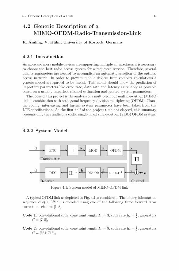
4.2 Generic Description of a Link 115
4.2 Generic Description of a
MIMO-OFDM-Radio-Transmission-Link
R. Amling, V. Kühn, University of Rostock, Germany
4.2.1 Introduction
As more and more mobile devices are supporting multiple air interfaces it is necessaryto choose the best radio access system for a requested service. Therefore, severalquality parameters are needed to accomplish an automatic selection of the optimalaccess network. In order to prevent mobile devices from complex calculations ageneric model is regarded to be useful. This model should allow the prediction ofimportant parameters like error rate, data rate and latency as reliably as possiblebased on a usually imperfect channel estimation and related system parameters.
The focus of this project is the analysis of a multiple-input multiple-output (MIMO)link in combination with orthogonal frequency-division multiplexing (OFDM). Chan-nel coding, interleaving and further system parameters have been taken from theLTE-specifications. As the first half of the project time has elapsed, this summarypresents only the results of a coded single-input single-output (SISO) OFDM system.
4.2.2 System Model
d
d
a
a
b
b
x
yn
H
ENC
DEC
OFDM
OFDM−1
MOD
DEMOD
Π
Π−1
Transmitter
ChannelReceiver
Figure 4.1: System model of MIMO-OFDM link
A typical OFDM link as depicted in Fig. 4.1 is considered. The binary informationsequence d ε{0, 1}Nd×1 is encoded using one of the following three forward errorcorrection schemes [1–3].
Code 1: convolutional code, constraint length Lc = 3, code rate Rc = 12, generators
G = [7; 5]8
Code 2: convolutional code, constraint length Lc = 9, code rate Rc = 12, generators
G = [561; 715]8
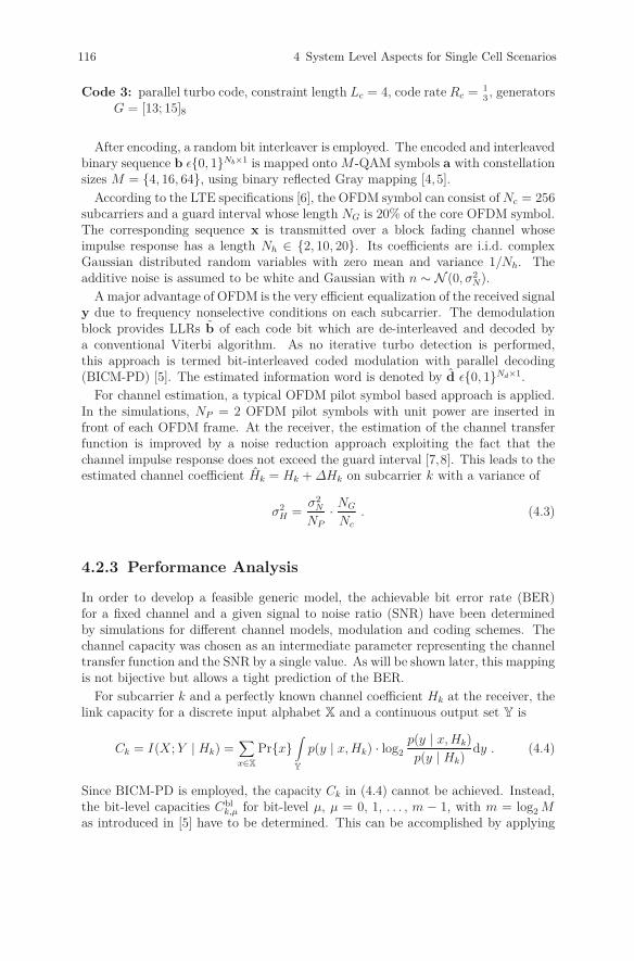
116 4 System Level Aspects for Single Cell Scenarios
Code 3: parallel turbo code, constraint length Lc = 4, code rate Rc = 13, generators
G = [13; 15]8
After encoding, a random bit interleaver is employed. The encoded and interleavedbinary sequence b ε{0, 1}Nb×1 is mapped onto M -QAM symbols a with constellationsizes M = {4, 16, 64}, using binary reflected Gray mapping [4, 5].
According to the LTE specifications [6], the OFDM symbol can consist of Nc = 256subcarriers and a guard interval whose length NG is 20% of the core OFDM symbol.The corresponding sequence x is transmitted over a block fading channel whoseimpulse response has a length Nh ∈ {2, 10, 20}. Its coefficients are i.i.d. complexGaussian distributed random variables with zero mean and variance 1/Nh. Theadditive noise is assumed to be white and Gaussian with n ∼ N (0, σ2
N).
A major advantage of OFDM is the very efficient equalization of the received signaly due to frequency nonselective conditions on each subcarrier. The demodulationblock provides LLRs b of each code bit which are de-interleaved and decoded bya conventional Viterbi algorithm. As no iterative turbo detection is performed,this approach is termed bit-interleaved coded modulation with parallel decoding(BICM-PD) [5]. The estimated information word is denoted by d ε{0, 1}Nd×1.
For channel estimation, a typical OFDM pilot symbol based approach is applied.In the simulations, NP = 2 OFDM pilot symbols with unit power are inserted infront of each OFDM frame. At the receiver, the estimation of the channel transferfunction is improved by a noise reduction approach exploiting the fact that thechannel impulse response does not exceed the guard interval [7,8]. This leads to theestimated channel coefficient Hk = Hk + ΔHk on subcarrier k with a variance of
σ2H =
σ2N
NP
· NG
Nc
. (4.3)
4.2.3 Performance Analysis
In order to develop a feasible generic model, the achievable bit error rate (BER)for a fixed channel and a given signal to noise ratio (SNR) have been determinedby simulations for different channel models, modulation and coding schemes. Thechannel capacity was chosen as an intermediate parameter representing the channeltransfer function and the SNR by a single value. As will be shown later, this mappingis not bijective but allows a tight prediction of the BER.
For subcarrier k and a perfectly known channel coefficient Hk at the receiver, thelink capacity for a discrete input alphabet X and a continuous output set Y is
Ck = I(X; Y | Hk) =∑x∈X
Pr{x}∫Y
p(y | x, Hk) · log2
p(y | x, Hk)
p(y | Hk)dy . (4.4)
Since BICM-PD is employed, the capacity Ck in (4.4) cannot be achieved. Instead,the bit-level capacities Cbl
k,μ for bit-level μ, μ = 0, 1, . . . , m − 1, with m = log2 Mas introduced in [5] have to be determined. This can be accomplished by applying

4.2 Generic Description of a Link 117
the chain rule of mutual information
Ck = I(b0, b1, . . . , bm−1; Y | Hk)
= I(b0; Y | Hk) + I(b1; Y | b0, Hk) + . . . + (4.5)
+ I(bm−1; Y | b0, b1, . . . , bm−2, Hk) .
Neglecting the constraint of known bit-levels leads to a reduction of the mutualinformation in (4.4) and the capacity for parallel decoding becomes
Cpdk = I(b0; Y | Hk) + I(b1; Y | Hk) + . . . + I(bm−1; Y | Hk) =
m−1∑μ=0
Cblk,μ < Ck . (4.6)
Finally, the average parallel-decoding capacity for an OFDM symbol with Nc
subcarriers and m bit-levels becomes
Cpd =1
Nc
Nc∑k=1
Cpdk =
1
Nc
Nc∑k=1
m−1∑μ=0
Cblk,μ . (4.7)
In order to infer from the bit-level capacities to the BER, simulations have beenperformed for different channel realizations, codes and modulation schemes. As anexample, Fig. 4.2 illustrates the obtained results for a 16-QAM and all consideredchannel impulse response lengths with uniform power delay profile.
0 1 2 3 4
10−4
10−3
10−2
10−1
100
0 1 2 3 4
10−4
10−3
10−2
10−1
100
0 1 2 3 4
10−4
10−3
10−2
10−1
100
a) Code 1 b) Code 2 c) Code 3
Cpd in bit/s/Hz →Cpd in bit/s/Hz →Cpd in bit/s/Hz →
BE
R→
BE
R→
BE
R→
simulatedsimulatedsimulatedxCy + z
x1C + y1x1C + y1
x2C + y2x2C + y2
rateraterate
Figure 4.2: Simulation results (gray), generated models (black) and for different FECcodes and 16-QAM
In Fig. 4.2a), the error rates for the simple convolution code show an exponentialslope with an increasing variance at higher capacities. For the convolution code withLc = 9 and the turbo code in the diagrams b) and c), a waterfall-like behavior canbe observed. Moreover, the turbo code’s BER can be predicted quite accurately asthe variations are very small even at high capacities. The largest capacities requiredfor a reference BER of 10−5 are 3.4 bit/s/Hz, 2.6 bit/s/Hz and 1.7 bit/s/Hz forcode 1, 2, and 3, respectively. Comparing these values with the spectral efficienciesR = m · Rc indicated by the dashed vertical lines, gaps ΔR(BER) = Cpd(BER) − Rcan be defined. They take the values 1.4 bit/s/Hz, 0.6 bit/s/Hz and 0.3 bit/s/Hz,

118 4 System Level Aspects for Single Cell Scenarios
respectively. As expected, the turbo code’s efficiency R approaches the capacity mostclosely. Further simulations have been performed for different modulation schemesand channels which cannot be shown in this survey. The modulation schemes 4-QAM and 64-QAM show a similar behavior as 16-QAM. The 4-QAM reaches aBER of 10−5 at 1.8 bit/s/Hz with code 1, 1.4 bit/s/Hz with code 2 and 1 bit/s/Hzwith code 3 and has smaller variations at low error rates. For 64-QAM, the BERvariations increase at higher capacities especially for the weak code 1. A BER of10−5 can be reached at capacities from 4 bit/s/Hz to 5 bit/s/Hz.
Figure 4.3 illustrates that the relationship between bit error rate and bit-levelcapacity does not depend on the length of the channel impulse response. For differentlengths Nh, the same quantitative behavior can be observed.
0 1 2 3 4
10−4
10−3
10−2
10−1
100
0 1 2 3 4
10−4
10−3
10−2
10−1
100
0 1 2 3 4
10−4
10−3
10−2
10−1
100a) Nh = 2 b) Nh = 10 c) Nh = 20
Cpd in bit/s/Hz →Cpd in bit/s/Hz →Cpd in bit/s/Hz →
BE
R→
BE
R→
BE
R→
Figure 4.3: Simulation results comparison for 16-QAM, Code 2 and different channelimpulse response lengths Nh
4.2.4 Generic Model
The aim of the project is to describe the dependency between the capacity Cpd
and the BER by a generic model. This is accomplished by applying curve fittingalgorithms to the results shown in Fig. 4.2. They provide results with a confidencelevel of 95%. For the code 1 with memory 2, an exponential function of the form
log10( BER(C) ) = x · Cy + z (4.8)
emerged as the best description. The function is depicted in Fig. 4.2a). The param-eters x, y and z are provided in Table 4.1 for 16-QAM modulation. For the othertwo codes, the curves were separated into two regions. The first region covers lowcapacities and high error rates, the second is the one of interest and includes thewaterfall region. In both of them, the logarithm of the BER can be approximatedby a straight line. We obtain
log10( BER1(C) ) = x1C + y1 for 0 < C < CP (4.9a)
log10( BER2(C) ) = x2C + y2 for CP < C < log2(M) , (4.9b)

4.2 Generic Description of a Link 119
where CP denotes the capacity where both lines intersect. Figures 4.2b) and c) illus-trate the results, the corresponding model parameters are summarized in Table 4.1.It also contains the gaps between the spectral efficiency R and the required capacityCpd predicted by the model.
Table 4.1: Generic model parameters for 16-QAM
Code 1 Code 2 Code 3
generic modellog10(BER(C)) x · Cy + z x1,2 · C + y1,2 x1,2 · C + y1,2
parameters region 1 x = −0.3689 x1 = −0.1085 x1 = −0.2340y = +2.1666 y1 = −0.2427 y1 = −0.3291z = −0.2958 - -
parameters region 2 - x2 = −4.4219 x2 = −17.1307- y2 = +5.7116 y2 = +22.9040
ΔR at 10−5 1.24 0.42 0.3
In order to use these models, the capacity Cpd needs to be computed using esti-mated channel coefficients Hk including errors ΔHk with a variance determined in(4.3)2. For codes whose BER curves exhibit a very high slope, capacity estimationerrors lead to dramatic prediction errors of the achievable error rate. This effectshall be investigated now. The channel estimation errors ΔHk are assumed to beindependent and complex Gaussian distributed. Including Hk into (4.6) leads to thefinal estimate Cpd = 1
Nc
∑Nck=1 Cpd
k .
An example for the distribution of Cpd at a target bit error rate 10−5 for FECcode 2 is illustrated in Fig. 4.4a) which corresponds to an average Es/N0 of 12.2 dB.Two OFDM pilot symbols are used for channel estimation with subsequent noisereduction. It can be observed that Cpd is nearly Gaussian distributed which couldbe expected since it stems from averaging over 256 subcarriers. The estimates’mean depends on the specific channel realization and is generally close to the truecapacity Cpd while the variance only depends on the signal to noise ratio of theoperating point of the specific BICM scheme. Hence, Cpd > Cpd holds in mostcases, i.e., the estimate is too optimistic and its application to resource allocationstrategies would lead to error rates larger than 10−5. Further investigations revealedthat the difference ΔCpd = Cpd − Cpd becomes not larger than 0.027 bit/s/Hz for95% of all estimated channels at the specific operating point of code 1, not largerthan 0.04 bit/s/Hz for the operating point of code 2 and 0.053 bit/s/Hz for code 3.The distance ΔCpd is getting smaller at high SNRs as can be seen from Fig. 4.4b)illustrating the maximum relative deviation of 95% of all channels. Considering aworst case scenario, an offset reducing Cpd by max95(ΔCpd) guarantees that 95%of all estimated capacities are not larger than Cpd. Otherwise, the model causes anoutage.
A second influence on the model quality is the variation of the required capacity
2It is assumed that the signal to noise ratio is perfectly known although this is a rather optimisticassumption.

120 4 System Level Aspects for Single Cell Scenarios
3.06 3.08 3.1 3.12 3.14 3.16 3.180
0.005
0.01
0.015
0.02
0.025
0.03
0.035
0.04
0 5 10 15 200
0.02
0.04
0.06
0.08
0.1
0.12
0.14
0.16a) histogram of Cpd b) ΔCpd over SNR
Cpd in bit/s/Hz → 10 log10(Es/N0) in dB →
max
95(Δ
Cp
d/C
pd)
p(Cpd)
Cpd
max95(Cpd)
ΔCpd
Figure 4.4: a): probability density of Cpd and true Cpd for operating point of code2, dashed red line indicates maximum of 95% of all Cpd, b): maximumof 95% of all ΔCpd/Cpd
Cpd at the target error rate. With respect to Fig. 4.2 the capacity varies at a BER of10−5 by ±0.25 bit/s/Hz for code 1 and by ±0.2 bit/s/Hz for code 2. The turbo codeshows nearly no variations. Again, a worst case consideration extracts the maximumrequired capacity to ensure the target BER. Moreover, channel estimation errors atthe receiver cause an additional loss which can be modeled by a complementarynoise term. This error causes small SNR degradations between 0.2 dB and 0.5 dBand, consequently, a small shift of the curves in Fig. 4.2 towards higher capacities.
4.2.5 Summary and Further Work
Simple generic models have been developed for a BICM-PD OFDM link describingthe dependency between the bit-level capacity and the error probability. These mod-els include different coding and modulation schemes related to LTE-specificationsbut can be easily generalized. Uncertainties due to estimation errors have been ana-lyzed and allow worst case scenarios with which the target error rate can be achievedin a predefined percentage of channels.
In a next step, the OFDM system shall be extended to a MIMO-OFDM system en-abling spatial multiplexing and different diversity methods like cyclic delay diversity.This extension requires the analysis of additional spatial parameters characterizingthe MIMO channel that have to be integrated into the generic models. Furthermore,automatic-repeat-and-request procedures shall be included into the investigations.
Bibliography
[1] 3GPP, 3rd Generation Partnership Project, Technical Specification Group RadioAccess Network, Multiplexing and channel coding (FDD) (Release 9), December2009, available: http://www.3gpp.org/ftp/Specs/html-info/25212.htm.
[2] M. Bossert, Kanalcodierung, Teubner, 2 edition, 1998.
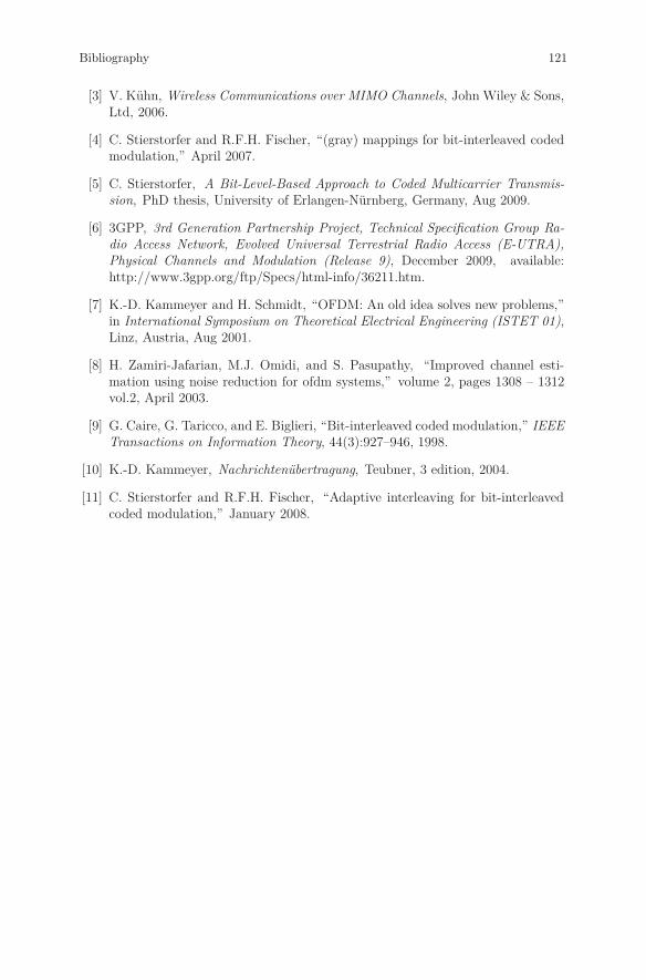
Bibliography 121
[3] V. Kühn, Wireless Communications over MIMO Channels, John Wiley & Sons,Ltd, 2006.
[4] C. Stierstorfer and R.F.H. Fischer, “(gray) mappings for bit-interleaved codedmodulation,” April 2007.
[5] C. Stierstorfer, A Bit-Level-Based Approach to Coded Multicarrier Transmis-sion, PhD thesis, University of Erlangen-Nürnberg, Germany, Aug 2009.
[6] 3GPP, 3rd Generation Partnership Project, Technical Specification Group Ra-dio Access Network, Evolved Universal Terrestrial Radio Access (E-UTRA),Physical Channels and Modulation (Release 9), December 2009, available:http://www.3gpp.org/ftp/Specs/html-info/36211.htm.
[7] K.-D. Kammeyer and H. Schmidt, “OFDM: An old idea solves new problems,”in International Symposium on Theoretical Electrical Engineering (ISTET 01),Linz, Austria, Aug 2001.
[8] H. Zamiri-Jafarian, M.J. Omidi, and S. Pasupathy, “Improved channel esti-mation using noise reduction for ofdm systems,” volume 2, pages 1308 – 1312vol.2, April 2003.
[9] G. Caire, G. Taricco, and E. Biglieri, “Bit-interleaved coded modulation,” IEEETransactions on Information Theory, 44(3):927–946, 1998.
[10] K.-D. Kammeyer, Nachrichtenübertragung, Teubner, 3 edition, 2004.
[11] C. Stierstorfer and R.F.H. Fischer, “Adaptive interleaving for bit-interleavedcoded modulation,” January 2008.

122 4 System Level Aspects for Single Cell Scenarios
4.3 Resource Allocation Using Broadcast
Techniques
M. Bossert, C. Huppert, J.G. Klotz, University of Ulm, Germany
4.3.1 Motivation
In the following we consider the downlink of a multi user communication system. Fortransmission in such a system the available resources, e.g., bandwidth and power,has to be allocated to the single users. This is often done by means of orthogonalaccess techniques, e.g., OFDMA, as in the uplink channel. However, the downlinkchannel is equivalent to the information theoretic broadcast channel since thereis only one sender transmitting messages to several receivers. In contrast to theuplink channel which can only be modeled as multiple access channel there is perfectsynchronization and coordination for transmitting messages in the downlink channel.Thus, using broadcast techniques as multiple access technique is superior in terms ofthe achievable rates. This was first shown by Cover in 1972 in [18]. He investigatedthe achievable rate region in the degraded broadcast channel and showed that allpoints of this region can be reached by means of superposition techniques.
4.3.2 Resource Allocation Algorithms
In multi-user OFDM systems the available subcarriers and the transmit-power mustbe allocated to the individual users in a way that certain service requirements arefulfilled. Motivated by the information theoretic superiority of broadcast techniquesover orthogonal access techniques, we consider resource allocation schemes for differ-ent requirements taking into account the broadcast gain in the following. Further-more, we do not only consider nodes equipped with a single antenna (SISO), but alsomulti antenna systems (MIMO). The optimal resource allocation schemes are knownfor all considered scenarios, however compared to the orthogonal methods it is morecomplex to determine their solutions and a larger signaling overhead is required toinform the users about the determined allocation. Thus, we propose strategies whichachieve a near optimum performance while requiring only a reasonable complexity.These strategies are based on one or more of the following techniques:
• Restriction to at most two users per carrier in order to keep the overhead low.
• Introduction of a new metric to predict interference caused by broadcast tech-niques (e.g. Eigenvalue Update).
• Usage of hybrid allocation strategies combining orthogonal access with broad-cast techniques.
In the following some of the proposed algorithms a briefly described and some sim-ulation results are presented.

4.3 Resource Allocation Using Broadcast Techniques 123
Sum-Rate Maximization
First, we consider a scenario where the overall system throughput, defined by thesum over all achievable user rates, is maximized under a transmit power constraint.The proposed algorithm uses eigen-beamforming and dirty paper coding, cf. [13].The inter-user interference is estimated and the eigenvalues of the affected beamsare updated (so-called ). Then the optimal power allocation is retrieved by performwater-filling over the adapted eigenvalues, cf. [19, 20]. In Fig. 4.5 the results of thealgorithm are compared with the optimal solution. It can be seen that the heuristicalgorithm achieves a sum rate of up to 99% of the optimal algorithm for low SNRs.For higher SNRs it still reaches 91%.
Sum-Rate Maximization with Minimum Rate Requirements
Like in the above considered scenario we maximize the sum rate of the system.However an individual minimum rate requirement for each user has to be fulfilled.Such a scheme may be needed in systems where delay critical as well as non-delaycritical data should be sent to each user.
Minimum Rate Requirements in SISO-OFDM systemsThe proposed algorithm, cf. [12], mainly works in two steps. First, a simple schedulerallocates one user to each carrier aiming in assigning the minimum rates. Thisscheduler performs the “worst selects” algorithm, i.e., always the instantaneous worstuser chooses its best carrier. In the second step, an additional user is added toeach suitable carrier by means of broadcast techniques. A modified version of thisalgorithm avoids irresolvable decoding dependencies in order to make it applicableto code words stretching over several blocks. Some simulation results of these twoalgorithms, named BC and DEP, are compared to the optimum solution, cf. [21,22],as well as to a pure scheduling strategy in Fig. 4.6. It can be seen that the proposedalgorithm achieves a performance near to the optimum and is clearly superior tothe pure scheduler. Furthermore, the results reveal that the modified version stillexploit a big part of the possible broadcast gain.
Minimum Rate Requirements in MIMO-OFDM systemsFor this problem two different heuristic resource allocation algorithms are proposed,cf. [14], which have a much lower complexity than the existing optimal solution,cf. [23]. The first strategy, extended eigenvalue update (EEU) algorithm, is based onthe previously discussed heuristic sum rate maximization algorithm using eigenvalueupdates. The second algorithm, the rate based coding (RBC) algorithm, makes useof the duality of uplink and downlink, which allows us to determine the allocation inthe dual uplink. The performance of these algorithms for different minimum ratescompared to the optimal algorithm is depicted in Fig. 4.7. It can be seen, thatthe EEU algorithm clearly outperforms the “simple scheduler”. The RBC algorithmachieves a better performance than the first algorithm at the cost of more complexity.Actually, it gets very close to the optimal solution for low required minimum rates.
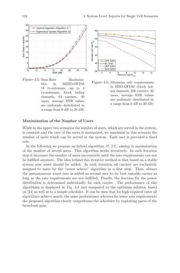
124 4 System Level Aspects for Single Cell Scenarios
−5 0 5 10 15 20 25 300
5
10
15
20
25
30
35
40
SNR [dB]
Sum
Rat
e in
bit/
s/H
z
Optimal Algorithm (Algorithm 1)Eigenvalue Update (Algorithm 2)
Figure 4.5: Sum-Rate Maximiza-tion in MIMO-OFDM(8 tx-antennas, up to 4rx-antennas, block fadingchannels, 64 carriers, 40users, average SNR valuesare uniformly distributed ina range from 0 dB to 20 dB)
2 4 6 8 10 12 1438
40
42
44
46
48
minimum rate Rmin
aver
age
user
rate
Rav
OPT SISOBC SISODEP SISOSCH SISO
Figure 4.6: Minimum rate requirementsin SISO-OFDM (block fad-ing channels, 256 carriers, 40users, average SNR valuesare uniformly distributed ina range from 0 dB to 20 dB)
Maximization of the Number of Users
While in the upper two scenarios the number of users, which are served in the system,is constant and the rate of the users is maximized, we maximize in this scenario thenumber of users which can be served in the system. Each user is provided a fixedrate.
In the following we propose an hybrid algorithm, cf. [11], aiming in maximizationof the number of served users. This algorithm works iteratively. In each iterationstep it increases the number of users successively until the rate requirements can notbe fulfilled anymore. The idea behind this iterative method is that based on a stablesystem new users should be added. In each iteration all carriers are exclusivelyassigned to users by the “worst selects” algorithm in a first step. Then, alwaysthe instantaneous worst user is added as second user to its best suitable carrier aslong as the rate requirements are not fulfilled. Finally, the fraction for the powerdistribution is determined individually for each carrier. The performance of thisalgorithms is displayed in Fig. 4.8 and compared to the optimum solution basedon [24] as well as to a simple scheduler. It can be seen that for high required rates allalgorithms achieve nearly the same performance whereas for lower rate requirementsthe proposed algorithm clearly outperforms the scheduler by exploiting parts of thebroadcast gain.
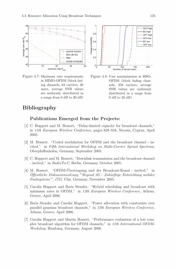
4.3 Resource Allocation Using Broadcast Techniques 125
0 10 20 30 4040
50
60
70
80
90
minimum rate Rmin
aver
age
user
rate
Rav
optimal solutionEEU (B=30)RBCsimple scheduler
Figure 4.7: Minimum rate requirementsin MIMO-OFDM (block fad-ing channels, 64 carriers, 20users, average SNR valuesare uniformly distributed ina range from 0 dB to 20 dB)
0 50 100 150 2000
0.2
0.4
0.6
0.8
1
Number of served users
Out
age
prob
abili
ty
SCH highBC highOPT highSCH lowBC lowOPT low
Figure 4.8: User maximization in SISO-OFDM (block fading chan-nels, 256 carriers, averageSNR values are uniformlydistributed in a range from0 dB to 20 dB)
Bibliography
Publications Emerged from the Projects:
[1] C. Huppert and M. Bossert, “Delay-limited capacity for broadcast channels,”in 11th European Wireless Conference, pages 829–834, Nicosia, Cyprus, April2005.
[2] M. Bossert, “Coded modulation for OFDM and the broadcast channel - in-vited,” in Fifth International Workshop on Multi-Carrier Spread Spectrum,Oberpfaffenhofen, Germany, September 2005.
[3] C. Huppert and M. Bossert, “Downlink transmission and the broadcast channel- invited,” in RadioTecC, Berlin, Germany, October 2005.
[4] M. Bossert, “OFDM-Übertragung und der Broadcast-Kanal - invited,” inÖffentliche Diskussionssitzung "‘Beyond 3G - Zukünftige Entwicklung mobilerFunksysteme"’, ITG, Ulm, Germany, November 2005.
[5] Carolin Huppert and Boris Stender, “Hybrid scheduling and broadcast withminimum rates in OFDM,” in 12th European Wireless Conference, Athens,Greece, April 2006.
[6] Boris Stender and Carolin Huppert, “Power allocation with constraints overparallel gaussian broadcast channels,” in 12th European Wireless Conference,Athens, Greece, April 2006.
[7] Carolin Huppert and Martin Bossert, “Performance evaluation of a low com-plex broadcast algorithm for OFDM channels,” in 11th International OFDM-Workshop, Hamburg, Germany, August 2006.
126 4 System Level Aspects for Single Cell Scenarios
[8] Carolin Huppert, Boris Stender, and Axel Hof, “Resource allocation for OFDMbroadcast channels allowing user-wise coding,” in 3rd International Symposiumon Wireless Communication Systems, Valencia, Spain, September 2006.
[9] Boris Stender, Carolin Huppert, and Gerd Richter, “Fast broadcasting,” In3rd International Symposium on Wireless Communication Systems, Valencia,Spain, September 2006.
[10] Carolin Huppert and Martin Bossert, “On achievable rates in the two userAWGN broadcast channel with finite input alphabets,” in IEEE InternationalSymposium on Information Theory, Nice, France, June 2007.
[11] C. Huppert and M. Bossert, “Heuristic approach of maximizing the number ofserved users in an OFDM broadcast channel,” in 12th International OFDM-Workshop, Hamburg, Germany, August 2007.
[12] C. Huppert and B. Stender, “Resource allocation with minimum rates forOFDM broadcast channels,” European Transactions on Telecommunications,18, No. 6:563–572, October 2007.
[13] J. Klotz, C. Huppert, and M. Bossert, “Heuristic resource allocation for sumrate optimization in MIMO-OFDM systems using eigenvalue updates,” inIEEE International Symposium on Wireless Communication Systems (ISWCS),Reykjavik, Iceland, October 2008.
[14] J. Klotz, F. Knabe, and C. Huppert, “Resource allocation algorithms for min-imum rates scheduling in MIMO-OFDM systems,” in 7th International Work-shop on Multi-Carrier Systems & Solutions (MC-SS 2009), Herrsching, Ger-many, May 2009.
[15] C. Huppert, F. Knabe, and J. Klotz, “User assignment for minimum raterequirements in OFDM-MIMO broadcast systems,” IET Electronic Letters, 45,No. 12:621–623, June 2009.
[16] J. G. Klotz, F. Knabe, and C. Huppert, “Resource allocation algorithms forminimum rates scheduling in MIMO-OFDM systems,” European Transactionson Telecommunications, 21, No. 5:449–457, August 2010.
[17] C. Huppert and J. Klotz, “Required transmit power applying Tomlinson-Harashima-precoding in scalar and MIMO broadcast systems,” IEEE Transac-tions on Communications, 2010. Accepted for publication.
Other References:
[18] T. M. Cover, “Broadcast channels,” IEEE Transactions on Information Theory,IT-18(1):2–14, January 1972.
[19] T. Michel and G. Wunder, “Optimal and low complex suboptimal transmis-sion schemes for MIMO-OFDM broadcast channels,” in IEEE InternationalConference on Communications, Seoul, Korea, May 2005.
Bibliography 127
[20] R. Böhnke, V. Kühn, and K.-D. Kammeyer, “Fast sum rate maximization forthe downlink of MIMO-OFDM systems,” in Canadian Workshop on Informa-tion Theory, Montreal, Canada, June 2005.
[21] T. Michel and G. Wunder, “Minimum rates scheduling for OFDM broadcastchannels,” in IEEE International Conference on Acoustics, Speech and SignalProcessing, volume 4, pages 41–44, Toulouse, France, May 2006.
[22] G. Wunder and T. Michel, “Optimal resource allocation for parallel Gaussianbroadcast channels: Minimum rate constraints and sum power minimization,”IEEE Transactions on Information Theory, 53(12):4817–4822, December 2007.
[23] G. Wunder and T. Michel, “Minimum rates scheduling for MIMO-OFDMbroadcast channels,” in 9th IEEE International Symposium on Spread Spec-trum Techniques and Applications, Manaus, Brazil, August 2006.
[24] D. N. C. Tse, “Optimal power allocation over parallel Gaussian broadcastchannels,” in IEEE International Symposium on Information Theory, Ulm,Germany, June 1997.

128 4 System Level Aspects for Single Cell Scenarios
4.4 Rate Allocation for the 2-user Multiple Access
Channel with MMSE Turbo Equalization
M. Grossmann, R. Thomä, Ilmenau University of Technology, Germany
4.4.1 Introduction
Recently, iterative (turbo) techniques have been recognized as practical solutions tomulti-user detection/equalization problems in coded communication systems. In [1],utilization of the optimal a posteriori probability (APP) equalizer in combinationwith the APP-based decoder is considered for turbo equalization in frequency-selective fading channels. In [2], the APP detector is replaced by a less compu-tational complex detector that performs soft canceling and minimum mean squarederror (SC MMSE) filtering. The turbo equalization technique for block-transmissionsover multiple-access channels (MACs) in [3] performs the equivalent signal process-ing in frequency domain (FD), further reducing the computational complexity.
The convergence of turbo systems can be analyzed by extrinsic information trans-fer (EXIT) charts [4]. Ashikhmin et al. [5] showed that for any code with rate R, thearea under its corresponding EXIT function is 1−R. Based on this area property ofthe EXIT chart, it has been shown in [6]- [8], that the problem of rate allocation inthe single-user or equal-rate multi-user turbo case, reduces to a simple curve-fittingproblem of the two-dimensional (2D) EXIT curves of the detector and decoder.
In this contribution, we consider the problem of rate allocation for the 2-userMAC in the presence of frequency-selective fading employing the low-complexity SCFD-MMSE turbo equalizer [3]. Specifically, we show that for such a turbo system,the equalizer EXIT characteristic is given by multidimensional surfaces, and thus,rate allocation to the users is no longer a simple 2D matching of the EXIT curves.Moreover, we derive an upper bound for the rate region of the turbo system, andstudy the problem of maximizing the sum rate of both users.
4.4.2 Turbo Equalization
Consider the cyclic prefix (CP) assisted U-user uplink system in Fig. 4.9, where abase station having M receive antennas receives signals from U active users, eachequipped with K transmit antennas. For the ease of analysis, we assume in thefollowing U = M = 2 and K = 1. However, the extension to more generic cases (U >2, M > 2, K > 1) is rather straightforward. The transmission scheme of the u-thuser (u = 1, 2) is based on bit interleaved coded modulation, where the informationbit sequence is independently encoded by a binary encoder, randomly bit-interleaved,binary phase-shift keying (BPSK) modulated, and grouped into several blocks thatare transmitted over the frequency-selective multiple-access MIMO fading channel.
At the receiver side, iterative processing for joint equalization and decoding isperformed. The receiver consists of an SC FD-MMSE equalizer and two single-user APP decoders. Within the iterative processing, the extrinsic LLR sequences{λu(n)} and {ζu(n)} of the coded bit sequences {bu(n)} are exchanged between the
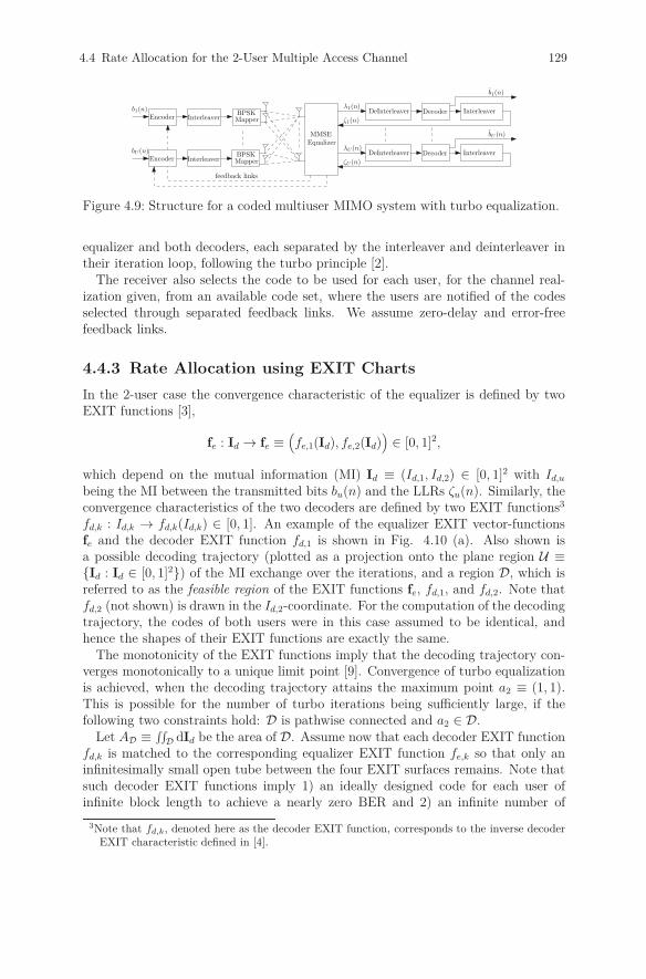
4.4 Rate Allocation for the 2-User Multiple Access Channel 129
Encoder InterleaverBPSKMapper
DeInterleaver Decoder Interleaver
MMSEEqualizer
λ1(n)
ζ1(n)
b1(n)
b1(n)
DeInterleaver Decoder InterleaverλU(n)
ζU(n)
bU (n)
Encoder InterleaverBPSKMapper
bU (n)
feedback links
Figure 4.9: Structure for a coded multiuser MIMO system with turbo equalization.
equalizer and both decoders, each separated by the interleaver and deinterleaver intheir iteration loop, following the turbo principle [2].
The receiver also selects the code to be used for each user, for the channel real-ization given, from an available code set, where the users are notified of the codesselected through separated feedback links. We assume zero-delay and error-freefeedback links.
4.4.3 Rate Allocation using EXIT Charts
In the 2-user case the convergence characteristic of the equalizer is defined by twoEXIT functions [3],
fe : Id → fe ≡(fe,1(Id), fe,2(Id)
)∈ [0, 1]2,
which depend on the mutual information (MI) Id ≡ (Id,1, Id,2) ∈ [0, 1]2 with Id,u
being the MI between the transmitted bits bu(n) and the LLRs ζu(n). Similarly, theconvergence characteristics of the two decoders are defined by two EXIT functions3
fd,k : Id,k → fd,k(Id,k) ∈ [0, 1]. An example of the equalizer EXIT vector-functionsfe and the decoder EXIT function fd,1 is shown in Fig. 4.10 (a). Also shown isa possible decoding trajectory (plotted as a projection onto the plane region U ≡{Id : Id ∈ [0, 1]2}) of the MI exchange over the iterations, and a region D, which isreferred to as the feasible region of the EXIT functions fe, fd,1, and fd,2. Note thatfd,2 (not shown) is drawn in the Id,2-coordinate. For the computation of the decodingtrajectory, the codes of both users were in this case assumed to be identical, andhence the shapes of their EXIT functions are exactly the same.
The monotonicity of the EXIT functions imply that the decoding trajectory con-verges monotonically to a unique limit point [9]. Convergence of turbo equalizationis achieved, when the decoding trajectory attains the maximum point a2 ≡ (1, 1).This is possible for the number of turbo iterations being sufficiently large, if thefollowing two constraints hold: D is pathwise connected and a2 ∈ D.
Let AD ≡ ∫∫D dId be the area of D. Assume now that each decoder EXIT function
fd,k is matched to the corresponding equalizer EXIT function fe,k so that only aninfinitesimally small open tube between the four EXIT surfaces remains. Note thatsuch decoder EXIT functions imply 1) an ideally designed code for each user ofinfinite block length to achieve a nearly zero BER and 2) an infinite number of
3Note that fd,k, denoted here as the decoder EXIT function, corresponds to the inverse decoderEXIT characteristic defined in [4].

130 4 System Level Aspects for Single Cell Scenarios
0 0.2 0.4 0.6 0.8 1
00.20.40.60.810
0.2
0.4
0.6
0.8
a3
fd,1
Id,1
a2
D
fe,2
a0Id,2
fe,1
I e,k
,k=
1,2
a1
decodingtrajectory
(a)
0.6 0.65 0.7 0.75 0.8 0.850.75
0.8
0.85
0.9
0.95
R1 [bpc]
R2
[bpc
]
V1
V2
Rmax = 1.62 bpc
(b)
Figure 4.10: (a) Equalizer EXIT functions fe,1 and fe,2 for a single random Rayleighchannel realization having L = 10 taps and decoder EXIT function fd,1
for a rate-1/2 convolutional code. (b) Rate region of the 2-user MACwith SC FD-MMSE turbo equalization for a single random channelrealization at Es/N0 = 5 dB, numerically computed by generating alarge number of different admissible convergence curves (a gray dotcorresponds to one curve).
turbo iterations. Under this assumption, the size of the area AD is close to zero andthe feasible region D can be characterized by a single curve, which is referred to asconvergence curve.
Let P be the set of admissible convergence curves in the plane region U , as de-fined in [10]. With the the area property of EXIT functions [5], we derive in astraightforward manner an upper bound for the rate region of both users, as
R ≡ ⋃p∈P
{(R1, R2) : Rk <
∫p
fe,l(Id)dId,k, k = 1, 2}
. (4.10)
Figure 4.10 (b) illustrates an example of the rate region in (4.10), where fe,1 andfe,2 have been computed for a random channel realization using the algorithm in [3].Note that the rate region in (4.10) is non-convex, in general, where the dominant faceof this region strongly depends on the particular realization of the equalizer EXITvector-function fe. Using the rate bound in (4.10), the problem of maximizing thesum rate of both users can be formulated as Rmax ≡ maxp∈P
∑2k=1
∫p fe,k(Id)dId,k.
Specifically, we show in [10] that this optimization problem can be efficiently solvedby using the Euler-Lagrange formalism [11]. As a result, the optimal decoder EXITcurves for both users with respect to the maximum sum rate of the turbo system,are obtained.
For practical reasons, however, each transmitter is restricted to have only a finitenumber of codes with fixed rates. For this scenario assumption, we propose in [10]a simple code selection algorithm for the rate allocation that maximizes the codingrate of each user, given the optimal decoder EXIT curve obtained from (4.10), whilesatisfying the constraints for successful decoding.
Figure 4.11 shows the average total throughput of the 2-user turbo system with theproposed code selection approach for frequency-selective Rayleigh fading channels

4.4 Rate Allocation for the 2-User Multiple Access Channel 131
having L = 32 taps. We assume sufficient long CP for inter-block interference tobe negligible. The binary-input sum capacity of the 2-user system is shown as areference. Also shown is the average total throughput performance for an automaticrepeat-request scheme with fixed coding rates of both users. For clarity, the ratesshown do not include the fractional rate loss incurred by the CP. As observed inFig. 4.11, substantial throughput gain is obtained with the proposed code selectionalgorithm over the fixed rate case. Further, we find that the throughput performanceis only 2 dB away (in the high Es/N0 region) from the theoretical limit.
−6 −4 −2 0 2 4 6 8 10 120
0.2
0.4
0.6
0.8
1
1.2
1.4
1.6
1.8
2
Es/N0 [dB]
Ave
rage
thro
ughp
ut [b
pc]
proposed methodBPSK capacity
Figure 4.11: Average total throughput of both users versus Es/N0 for the proposedrate allocation scheme using the rate-compatible punctured serial con-catenated convolutional codes in [12], and for automatic repeat-requestwith fixed coding rates r1/2 = 0.1 · n with n = 1, .., 9 (dashed curves,from bottom to top).
4.4.4 Summary
In this contribution, we consider the problem of rate allocation in the frequency-selective 2-user Gaussian multiple-access fading channel employing a low complexityMMSE turbo equalizer. We derive an upper bound on the rate region of the turbosystem and study the problem of maximizing the sum rate of both users. In addition,numerical results of a simple code selection algorithm for rate allocation to both usersare presented.
Bibliography
[1] C. Douillard, et al., “Iterative correction of intersymbol interference: Turboequalization,” European Trans. Telecomm., vol. 6, no. 5, pp. 507-511, Sept. 1995.
132 4 System Level Aspects for Single Cell Scenarios
[2] X. Wang, and H. V. Poor, “Iterative (turbo) soft interference cancellation anddecoding for coded CDMA,” IEEE Trans. Commun., vol. 47, no. 7, pp. 1046-1061, July 1999.
[3] K. Kansanen, and T. Matsumoto, “An analytical method for MMSE MIMOturbo equalizer EXIT chart computation,” IEEE Trans. Wireless Commun., vol.6, no. 1, pp. 59-63, Jan. 2007.
[4] S. ten Brink, “Convergence behavior of iteratively decoded parallel concatenatedcodes,” IEEE Trans. Commun., vol. 49, no. 10, pp. 1727-1737, Oct. 2001.
[5] A. Ashikhmin, G. Kramer, and S. ten Brink, “Extrinsic information transferfunctions: model and erasure channel properties,” IEEE Trans. Inform. Theory,vol. 50, no. 11, pp. 2657-2673, Nov. 2004.
[6] S. ten Brink, G. Kramer, and A. Ashikhmin, “Design of low-density parity-checkcodes for modulation and detection,” IEEE Trans. Commun., vol. 52, no. 4, pp.670-678, April 2004.
[7] A. Sanderovich, M. Peleg, and S. Shamai (Shiz), “LDPC Coded MIMO MultipleAccess With Iterative Joint Decoding,” IEEE Trans. Inform. Theory, vol. 51,no. 4, pp. 1437-1450, April. 2005.
[8] A. Roumy, and D. Declercq, “Characterization and Optimization of LDPC Codesfor the 2-User Gaussian Multiple Access Channel,” EURASIP Journal on Wire-less Commun. and Netw., vol. 2007, Article ID 74890, 10 pages, 2007.
[9] F. Brännström, L.K. Rasmussen, and A.J. Grant, “Convergence analysis and op-timal scheduling for multiple concatenated codes,” IEEE Trans. Inform. Theory,vol. 51, no. 9, pp. 3354-3364, Sept. 2005.
[10] M. Grossmann, T. Ortlepp, T. Matsumoto, “Rate Allocation for 2-User MACwith MMSE Turbo Equalization,” IEEE Trans. on Wireless Commun., vol. 5,pp. 1033-1043, March 2010.
[11] J. Jost, and X. Li-Jost, “Calculus of variations,” Cambridge Studies in AdvancedMathematics, vol. 64, Cambridge University Press, Cambridge, 1998.
[12] M. Tüchler, “Design of serially concatenated systems depending on the blocklength,” IEEE Trans. Commun., vol. 52, no. 2, pp. 209-218, Feb. 2004.

4.5 Coexistence of Systems 133
4.5 Coexistence of Systems
F. K. Jondral, U. Berthold4, Karlsruhe Institute of Technology (KIT),GermanyM. Schnell, S. Brandes, DLR, Germany
The efficiency of spectrum usage for a radio communications system employinga fixed bandwidth is measured as the average number of bits that are transmittedper second and per Hertz in a certain area. For simplicity reasons we will use thenotion spectrum efficiency instead of efficiency of spectrum usage here. The resultsof measurement campaigns recently accomplished, pointed out that, even in heavilyoccupied bands, usually not more than fifteen percent of the spectral resource iseffectively employed. This leads to the justifiable assumption that dynamic accessupon the transmission resource will at least contribute to a reduction of spectrumscarcity.
The TAKOKO5 project within TakeOFDM dealt with the utilization of resourcesleft idle in the frequency band allocated to a primary system of authorized users(so-called spectrum holes in the time-frequency-plane) by an overlay system of sec-ondary users. A coexistence strategy is investigated that explicitly harnesses theflexibility of the OFDM (orthogonal frequency-division multiplexing) method withrespect to spectrum utilization. I.e. an OFDM-based overlay system is installed inorder to enhance the spectrum efficiency within the frequency region allocated to anauthorized primary user system.
As a starting point of our investigations, frequency regions as well as primary usersystems appearing capable for additional use by an overlay system were identified.These are essentially systems employing the resource by FDMA (frequency divisionmultiple access) or TDMA (time division multiple access). Table 4.2 provides anoverview over the scenarios adopted.
Table 4.2: Overviews over scenarios adoptedScenario 1 Scenario 2 Scenario 3
Frequency region VHF band 960 - 1215 MHz 1800 MHz
Primary system Aircraft radio Distance MeasuringEquipment (DME)
GSM
Overlay system WLAN for communi-cation at airports
Flexible mobile commu-nication system
Metropolitan AreaNetwork (MAN)
Special aspects Interference suppres-sion
Detection of spectrumholes, suppression ofjammers
Utilization of spec-trum holes
Reliable detection of idle resources in the time-frequency-plane, i.e., the detectionof primary user signals by the overlay system, as well as the signalization of theresults within the overlay systems are of paramount importance for the acceptanceof overlay systems by primary users.
4Dr.-Ing. Ulrich Bertold is now an employee of COMSOFT GmbH, Karlsruhe.5TAKOKO is an acronym for technologies, algorithms, and concepts for OFDM systems coexisting
with authorized systems in the same frequency band

134 4 System Level Aspects for Single Cell Scenarios
spectrum hole
licensed system
time
Figure 4.12: Idle resources represented by spectrum holes
The impact that the overlay has on the primary system has to be kept minimum.Therefore, detection as well as false alarm probabilities for the detection of primaryusers’ signals by the overlay system were derived. In the course of the work it becameevident that only the application of a detection algorithm distributed over the overlaysystem’s stations is able to guarantee sufficiently high detection probabilities and atthe same time lead to tolerable false alarm rates.
Moreover, an efficient signaling within the overlay system of the spectrum utiliza-tion by the primary system proves to be important in order to optimally make useof the spectrum holes.
Employing OFDM in overlay systems, of course, also implicates some disadvan-tages. Among these disadvantages are the strong spurious transmissions that maylead to disturbances in the primary system. To reduce them, in addition to wellknown methods, like windowing of the transmitted signal in the time domain or theintroduction of guard bands, subcarrier weighting, the application of cancellationcarriers as well as a combination of windowing and cancellation carriers were inves-tigated in TAKOKO. In scenario 1, for example, it was shown that the applicationof this combination may reduce the energy level contained in a secondary lobe to avalue of 50 dB below the OFDM signal energy level. The new techniques for distur-bance suppression were integrated into the simulation model of an adaptive OFDMtransmitter.
At the receiver side of an overlay system’s user the desired signal is superim-posed by interferences generated by the primary system. Although the channelsoccupied by primary system’s users are generally not employed by the overlay sys-tem, the overlay system’s performance is influenced by these interferences. In thisconnection, interference reduction methods concerning narrow band interferers wereinvestigated with respect to scenario 1. Here time domain windowing of the re-ceived signal as well as the frequency domain estimation of the interfering signalwere applied. High quality results were achieved with a combination of time domainwindowing and leakage compensation in the frequency domain. The interferenceminimization techniques were integrated into the overlay system’s receivers. To fa-cilitate a dynamic adaptation to varying interference situations, the OFDM framestructure had to be modified by introducing observation carriers such that theirposition may be adjusted to the actual spectrum occupancy.
Further essential aspects of the TAKOKO project were the investigation of therequirements on the MAC (medium access control) layer as well as the specificationof an adequate MAC protocol. Here the essential assumption was that the overlay
4.5 Coexistence of Systems 135
system operates as an ad-hoc network, i.e., without central coordination. There-fore, all individual stations are equal and the MAC protocol has to incorporate thesystem’s distributed character. In order to be able to initiate a data transmissionthe stations essentially need a) knowledge about the frequency occupation by theprimary system (overlay feature) and b) information about those stations in theirenvironment to which it is possible to establish a connection (ad hoc feature). Fordetermination of the primary system’s frequency occupation measurements are per-formed periodically. The measurement periods for the overlay system’s stations haveto be coordinated because no overlay system’s stations should radiate signals thento guarantee a reliable detection of primary system signals. Exactly this coordi-nation is assumed by the AHO-MAC (ad hoc overlay MAC) protocol developed inthe TAKOKO project. Similar to PRMA (packet reservation multiple-access), asmany time slots for data transmission as mini slots for acknowledgments are pro-vided. Moreover, special time slots for occupancy measurements and for the mutualsynchronization of the overlay stations are defined.
The representation of the frequency utilization by the primary system in form ofthe occupancy vector plays an important role within the overlay system and affectsthe PHY (physical) as well as the MAC layer. Therefore, an approach of crosslayer optimization was chosen. Here the layered model was kept but the interfacesbetween the layers were extended by the definition of more detailed as well as morespecific parameters.
In summary promising methods were developed in TAKOKO which show thatin principle OFDM based overlay systems may be implemented. Although theTAKOKO approaches were considered with respect to preferably realistic overlayscenarios (Table 4.2), further investigations have to be performed before OFDMbased overlay systems may be practically implemented. Those investigations couldnot be accomplished within the project because of the given time and effort con-straints and because they were beyond the project’s objectives. Moreover, the realimplementation of OFDM based overlay systems requires fundamental decisions inthe political as well as in the regulatory area in order to define the principle frame-work. The scientific results acquired in the TAKOKO project are essentially sum-marized in the doctoral dissertations [1] and [2]6.
Bibliography
[1] U. Berthold, Dynamic Spectrum Access Using OFDM-based Overlay Systems,Dissertation, Forschungsberichte aus dem Institut für Nachrichtentechnik derUniversität Karlsruhe (TH), Band 21, Karlsruhe, 2009.
[2] S. Brandes. Suppression of Mutual Interference in OFDM Based Overlay Sys-tems, Dissertation, Forschungsberichte aus dem Institut für Nachrichtentechnikder Universität Karlsruhe (TH), Band 22, Karlsruhe, 2009.
6Both dissertations may be downloaded from www.cel.kit.edu
136 4 System Level Aspects for Single Cell Scenarios
4.6 System Design for Time-Variant Channels
P. Klenner, S. Vogeler, K.-D. Kammeyer, University of Bremen, Ger-manyL. Reichardt, S. Knörzer, J. Maurer, W. Wiesbeck, University of Karl-sruhe, Germany
The following two subsections summarize the cooperation between the Arbeits-bereich Nachrichtentechnik (ANT) at the University of Bremen and the Institutfür Hochfrequenztechnik und Elektronik (IHE) at the University Karlsruhe. Bothpartners were engaged in two projects within the DFG program ”TakeOFDM”. Theproject titles coincide with the names of the following sections. The focus is in Sec-tion 4.6.1 on SIMO (Single-Input-Multiple-Output)-OFDM and in Section 4.6.2 onMIMO (Multiple-Input-Multiple-Output)-OFDM in rapidly fading channels, whichare modeled by ray-optic methods to include realistic propagation effects.
4.6.1 Multicarrier Systems for Rapidly Moving Receivers
In this section, the use of multicarrier systems and, in particular, OFDM for high-rate wireless data transmission and for fast moving receivers mounted on high-speedtrains, cars, or airplanes is considered. Realizing high data rates at simultaneouslyhigh mobility is a difficult feat for any communication system. If broadband signalingfor a high data rate causes the sample duration to become smaller than the channel’smaximal echo duration, then OFDM can simplify the resulting equalization effort.But a frequency-selective channel is only separated into orthogonal parallel subcar-riers in the case of a time-invariant channel, i.e., if the channel remains unchangedduring one OFDM symbol. High mobility environments, however, are characterizedby time-invariant channels, which leads to a loss of the subcarriers’ orthogonality.Intercarrier interference (ICI) occurs, the equivalent to intersymbol interference intime-domain.In the simplest case, ICI can be modeled as a source of noise in addition to thethermal noise. Neglecting it results in a degradation of the achievable bit-error rate.More dramatic is the impact, if the channel is changing so fast, that the violationof the sampling theorem prevents a reliable channel estimation. This case does notnecessarily occur due to extreme speed, but also due to a large pilot symbol spacing.
The observations conducted here refer to a system for a high-speed train in a singlefrequency network. The channel model described in Section 2.2.2 is applicable todifferent frequencies and is transferable to other types of mobiles. Similarly, theconsiderations apply to the Doppler effect for other types of fast moving receivers.For an extensive investigation under realistic channel conditions, the project is basedon modeling the propagation conditions via ray-tracing methods by which a seriesof channel impulse response is computed.
Subsequently, three main strategies will be discussed with the aim to solve theconflict between the transmission channel’s high time and frequency selectivity: Theapplication of a pre-equalizer to shorten the channel impulse response, the use ofsoft impulse shaping for a non-orthogonal multicarrier system, and multi-antennaconcepts to reduce the Doppler spread.
4.6 System Design for Time-Variant Channels 137
During the project, parameters of an OFDM system were defined taking into ac-count the main characteristics of the channel that was determined by ray-tracingsimulations. The system’s performance limits were established through Monte Carlosimulations. The system parameters have been dimensioned such that the time-bandwidth conflict caused by the interference is completely focused on the frequencydomain, while time domain intersymbol interference is avoided. Thus, the proce-dures to counter the Doppler effect can be performed after the DFT in the receiver.
By consolidating the effects of multipath and Doppler spread in the form of achannel matrix, a linear equalization of both effects according to the MMSE crite-rion can be carried out. The disadvantage of this procedure, however, is a relativelyhigh computational effort, while the knowledge of the signal alphabet is not ex-ploited. Therefore, two well-known algorithms for low-complex equalization wereimplemented: a successive linear MMSE equalizer and a successive equalizer withdecision feedback structure, which were modified in accordance to the requirementsof the scenario. Both methods, however, did not provide satisfactory simulationresults, which in the decision-feedback method is due to the suboptimal detectionsequence. This called for the sorted QR decomposition (SQRD) employed in V-BLAST to improve the detection sequence. This resulted in the best detectionperformance, but at the cost of a comparably high computational effort. Throughthe gradual decomposition of the channel matrix in submatrices the effort can bereduced significantly, yielding a trade-off between high performance and low com-plexity equalization. This successive SQRD is detailed in [11, 12].
As part of the investigations of alternative multicarrier concepts the subcarrierspectra of OFDM were replaced by soft non-orthogonal pulse shapes, i.e., time-limited Gaussian pulses. In the frequency domain, this leads to a concentration ofinterference power in the vicinity of the main diagonal of the channel matrix. Thisin turn has a positive effect on the performance of the aforementioned equalizationmethods, particularly for the low-complex variants such as the successive SQRD. Thesoft impulse shaping also allowed for Maximum Likelihood detection with reasonableeffort, because the concentration of the interference power allows the use of a time-variant Tailbiting-MaxLogMAP algorithm with a reduced number of states. Thisprocedure resulted in the best compromise between complexity and performance ofthe transmission system [13].
Shortening the channel impulse response potentially allows for a shorter OFDMsymbol, which is beneficial in rapidly time-varying environments. Numerous well-known non-blind and blind algorithms for computing equalizer coefficients were in-vestigated regarding their applicability in the scenarios. It turned out that thesemethods produce either ill-conditioned frequency responses or that the convergencespeed is not sufficient in case of the blind methods.
Multi-antenna concepts open up the spatial domain to procure Doppler spreadcompensation. Sectorizing antennas exploit the relationship between the impingingwaves’ angle of incidence and their resulting Doppler shift. By restricting the rangeof angles of incidences a sectorizing antenna simultaneously reduces the effectiveDoppler spread compared to a omnidirectional antenna without any restriction of theincidence angle. One practical implementation is beamforming via a Uniform LinearArray (ULA), and the beams are formed such that the Doppler spread is equally
138 4 System Level Aspects for Single Cell Scenarios
distributed among all beams [2]. Furthermore, a ULA can be used for a methodcalled spatial interpolation, in which the signals of the individual antenna elementsare filtered by a time-variant interpolator such that the filter output resembles theoutput of a time-invariant channel [3].
The two scenarios of a noise barrier and vegetation are considered as typical highspeed lines. The radio channel has very different properties, therefore, these scenar-ios are used as a reference. Details can be found in [6,8,9]. For the simulation of wavepropagation, a three dimensional ray-propagation model is employed. It providescharacteristic parameters for each multipath, from which the sequence of channelimpulse responses and channel characteristics are extracted. The wave propagationmodel takes into account the propagation phenomena of reflection, diffraction andscattering. The approach to modeling the distribution of vegetation is described in2.2.2.
Figure 4.13 shows the BER performance for a SIMO-OFDM system with receivediversity in a rapidly fading channel (one transmit and two or four receive antennas,Nt = 1, Nr = 2, 4). For omnidirectional reception widely spaced antennas are used,which yield completely uncorrelated channels per antenna. Without any means ofDoppler compensation this results in the worst performance. Sectorizing antennasand spatial interpolation based on a ULA with interantenna spacing d/λ yield abetter performance. Sectorization is here achieved by forming two beams in andagainst the direction of the movement. Spatial interpolation is achieved by com-puting two virtually non-moving antennas, which fix the channel over the middleof the respectively received OFDM signal. The received signals on the resultingvirtual antennas are correlated. Taking this correlation into account by means of awhitening matched filter (WMF) improves the performance over the matched filter(MF).
4.6.2 Highly Mobile MIMO-OFDM-Transmission inRealistic Propagation Scenarios
Doppler spread compensating antenna structures at the receiver offer an efficientapproach to solve the problem of the channel’s time-variance already in time-domain.The focus now is on the two antenna configuration discussed in Section 4.6.1, whosefunction ultimately is to affect a less rapidly fading channel prior to the DFT.Unlike the previous discussion, where a single transmit antenna was employed, inthe following the focus is shifted to the transmitter side.
The MIMO philosophy is based on two pillars: Spatial transmit diversity is pro-vided by Space-Time codes, and spatial multiplexing allows to increase the data rateby transmitting independent data streams. The development of these techniques isshaped by the assumption of a time-invariant channel, and most methods even de-mand that. In the following, the mutual benefit of MIMO-signaling and Dopplerspread compensation measures is described. If the Doppler spread is small, then theloss of time diversity can be made up by spatial diversity, and if the Doppler spreadis large, then the Doppler compensating antennas can effect a less time-invariantchannel such that the MIMO-signal processing upholds its validity [1, 4].Rapid channel fluctuations in conjunction with multiple transmit antennas pose the

4.6 System Design for Time-Variant Channels 139
0 5 10 15 20 25 30 35 4010−4
10−3
10−2
10−1
100
Eb/N0 in dB
BE
Ra) Nt = 1, Nr = 2
omni,MF
sec,MF
sec,WMF
SI,MF
SI,WMF
0 5 10 15 20 25 30 35 4010−4
10−3
10−2
10−1
100
Eb/N0 in dB
BE
R
b) Nt = 1, Nr = 4
omni,MF
sec,MF
sec,WMF
SI,MF
SI,WMF
Figure 4.13: BER-performance for SIMO-OFDM with a single transmit antenna anddifferent receiver configurations: omnidirectional antennas with widelyspaced antennas, sectorizing antennas and spatial interpolation basedon a ULA, parameters: 256 subcarriers, 16QAM, exp. power delayprofile, antenna spacing d/λ = 0.25, Doppler spread fDTs = 0.2, raisedcosine filters (r = 0.18), zero forcing channel est.
possible disadvantage of decreased bandwidth efficiency, in that frequent trainingbecomes necessary. However, since the channel is forced to become less rapidlyfading by Doppler compensating measures the pilot spacing in time direction canbecome larger. Similarly, noncoherent ST codes can profit from a channel that doesnot change too much during a signaling interval.
During the course of the project it is investigated how the functions of Dopplercompensation and the separation of data streams using multiple receiving antennascan be combined. One possibility is the use of multiple spatially separated antennaarrays, each used for Doppler compensation, followed by the recovery of the trans-mitted data streams.
Parameter estimation is a further important issue. In particular, the channel’sautocorrelation function needs to be estimated, since the receiver requires it in orderto perform the spatial interpolation. The idealized assumption of the Bessel functionas autocorrelation holds only in isotropic scattering environments. Other scatteringconditions and mutual antenna coupling lead to different correlations. Realisticchannels already studied lead to an SNR loss. It is possible to find an estimate ofthe ACF based on the cyclic OFDM signal structure without spending extra trainingdata [5].
Furthermore, the optimization of antenna structures for the purpose of minimizingthe mutual antenna coupling is considered. The algorithms used for data processingin the baseband yield a better performance if the individual antennas for sectoriza-tion or spatial interpolation are decoupled. This condition is violated in practicalsystems, since the individual antenna elements are positioned very close to eachother, so that inevitably crosstalk of the antennas occurs. The effect of mutual cou-

140 4 System Level Aspects for Single Cell Scenarios
pling and its minimization and compensation are investigated, so that the idealizedassumptions of the baseband processing can be maintained.
The consideration of realistic channel models as a benchmark of these approachesrepresents a further focus of the project. Two scenarios are considered, a high-speed train and vehicle-to-vehicle environments. In the former, the propagationconditions are dominated by a major incident direction (by the base stations alongthe railroad tracks), while in the latter, in principle, all incidence directions arepossible. Regarding the car-to-car scenario, a further challenge is to find Dopplercompensating antenna structures, which are not impaired by the car structure.
Figure 4.14 shows the BER performance for a (2×2)-MIMO OFDM systems withthe receiver configurations known from Fig. 4.13. In Fig. 4.14a transmit diversityis provided by the Alamouti Space-Time code, whereas in Fig. 4.14b the V-BLASTis employed, i.e., independent data streams are transmitted from both transmitantennas. For a fair comparison identical data-rates are used, i.e., 16QAM forthe Alamouti scheme, and QPSK for V-BLAST. Comparing the two-fold transmitdiversity scheme in Fig. 4.14a with the single transmit diversity case in Fig. 4.13ashows that except for spatial interpolation the gains promised by two-fold transmitdiversity are small. This can be attributed to the channel estimation which needs todetermine twice as many channel parameters. On the other hand, the gains for V-BLAST in employing Doppler compensating antenna structure are more impressive.
0 5 10 15 20 25 30 35 4010−4
10−3
10−2
10−1
100
Eb/N0 in dB
BE
R
a) Nt = 2, Nr = 2, Alamouti
omni,ZF
omni,ML
sec,ZF
sec,ML
SI,ZF
SI,ML
0 5 10 15 20 25 30 35 4010−4
10−3
10−2
10−1
100
Eb/N0 in dB
BE
R
b) Nt = 2, Nr = 2, VBLAST
omni,ZF
omni,ML
sec,ZF
sec,ML
SI,ZF
SI,ML
Figure 4.14: BER-performance for (2 × 2)-OFDM and different receiver configura-tions: omnidirectional antennas with widely spaced antennas, sector-izing antennas and spatial interpolation based on a ULA, parameters:256 subcarriers, 16QAM (a) and QPSK (b), exp. PDP, d/λ = 0.25,fDTs = 0.2, RC-filters (r = 0.18), ZF channel est.
Bibliography
[1] K.-D. Kammeyer and P. Klenner, “Space-Time Coded OFDM Transmissionwith Spatial Interpolation in the Presence of Severe Doppler Spread,” in 3rd
Bibliography 141
International Symposium on Communications, Control and Signal Processing(ISCCSP 08), St. Julians, Malta, March 2008.
[2] P. Klenner and K.-D. Kammeyer, “Doppler-Compensation for OFDM-Transmission by Sectorized Antenna Reception,” in 6th International Workshopon Multi-Carrier Spread Spectrum (MCSS 07), Herrsching, Germany, May 2007.
[3] P. Klenner and K.-D. Kammeyer, “Spatially Interpolated OFDM with ChannelEstimation for Fast Fading Channels,” in IEEE Vehicular Technology Confer-ence 2007 (VTC2007-Spring), Dublin, Ireland, April 2007.
[4] P. Klenner and K.-D. Kammeyer, “Performance of Space-Time-Coded OFDMwith Sectorized Antenna Reception,” in International ITG/IEEE Workshop onSmart Antennas (WSA 08), Darmstadt, Germany, Feb. 2008.
[5] P. Klenner and K.-D. Kammeyer, “Temporal Autocorrelation Estimation forOFDM with Application to Spatial Interpolation,” in Asilomar Conf. on Sig-nals, Systems and Computers, Monterey, CA, Oct. 2008.
[6] S. Knörzer, Funkkanalmodellierung für OFDM-Kommunikationssysteme beiHochgeschwindigkeitszügen, PhD thesis, University Karlsruhe, Germany, 2009.
[7] S. Knörzer, J. Maurer, T. Fügen, and W. Wiesbeck, “Wave Propagation Mod-eling for Communication between Moving Vehicles,” in National Radio ScienceMeeting, Boulder, USA, Jan 2005.
[8] S. Knörzer, J. Maurer, S. Vogeler, K.-D. Kammeyer, and W. Wiesbeck, “Chan-nel Modeling and Characterization for High-Speed Train OFDM Systems,” inCOST 273 TD(05)086, Leuven, Belgium, June 2005.
[9] S. Knörzer, J. Maurer, S. Vogeler, K.-D. Kammeyer, and W. Wiesbeck, “Chan-nel modeling for a high-speed train ofdm communication link supporting highdata rates,” in Proc. 5th Int. Conf. on ITS Telecomm. 2005, pages 333–336,Brest, France, June 2005. Best Student Paper Award.
[10] J. Maurer, S. Knörzer, and W. Wiesbeck, “Ray Tracing in Rich ScatteringEnvironments for Mobile-to-Mobile Links,” in Proc. of the Int. Conf. on Elec-tromagnetics in Advanced Applications, Italy, Sept. 2005.
[11] S. Vogeler, Verfahren zur Kompensation von Doppler-Einflüssen in Mehrträger-Übertragungssystemen, PhD thesis, University of Bremen, Germany, 2006.
[12] S. Vogeler, L. Brötje, P. Klenner, V. Kühn, and K.-D. Kammeyer, “IntercarrierInterference Suppression for OFDM Transmission at Very High Velocities,” in9th International OFDM-Workshop (InOWo 2004), Dresden, Germany, Sept.2004.
[13] S. Vogeler, P. Klenner, and K.-D. Kammeyer, “Multicarrier Transmission forScenarios with High Doppler Influence,” in 10th International OFDM-Workshop(InOWo 2005), Hamburg, Germany, Aug. 2005.
142 4 System Level Aspects for Single Cell Scenarios
4.7 Combination of Adaptive and Non-Adaptive
Multi-User OFDMA Schemes in the Presence
of User-Dependent Imperfect CSI
A. Kühne, A. Klein, Technische Universität Darmstadt, Germany
4.7.1 Introduction
The Orthogonal Frequency-Division Multiple Access (OFDMA) transmission schemeis a promising candidate for future mobile networks. It offers an efficient adaptationto the channel conditions by performing a time-frequency scheduling of the differ-ent subcarriers to the different users. However, Channel State Information (CSI)is required at the transmitter in order to perform such an adaptive scheduling inan optimal way. Having perfect CSI for all users at the Base Station (BS), theuse of frequency adaptive OFDMA schemes achieves very good performances byexploiting multiuser diversity . Having no CSI at all at the BS, the use of frequencynon-adaptive OFDMA schemes exploiting frequency diversity independently fromany CSI is the best strategy, however, not achieving the performance of adaptiveschemes with perfect CSI . For the case of imperfect CSI, only pure adaptive OFDM-based systems have been studied in the literature but not a combination of adaptiveand non-adaptive transmission modes. A comparison of adaptive and non-adaptivemultiuser OFDMA schemes in the presence of imperfect channel knowledge has beeninvestigated assuming the same degree of CSI imperfectness for each user [1]- [5]. Itappears that at a certain level of CSI imperfectness, it is beneficial to switch fromadaptive to non-adaptive transmission, i.e., depending on the quality of the channelknowledge, either all users apply the adaptive or non-adaptive transmission mode.In a realistic scenario however, the level of CSI imperfectness differs from user touser, i.e., for some users, the CSI is only slightly corrupted, whereas for other users,the CSI is totally inaccurate. Hence, we propose a hybrid OFDMA scheme whereboth adaptive and non-adaptive transmission schemes co-exist at the same timeand show how to optimally combine these transmission schemes in the presence ofuser-dependent imperfect CSI [6].
4.7.2 Combining Transmission Schemes
In the considered hybrid OFDMA scheme, different users are served either adap-tively or non-adaptively sharing the available bandwidth. Applying the non-adaptiveOFDMA transmission scheme, a fixed modulation and subcarrier allocation is per-formed. This scheme does not rely on instantaneous CSI but exploits frequencydiversity. Applying the adaptive OFDMA transmission scheme, an adaptive sub-carrier allocation together with an adaptive modulation based on the instantaneousCSI is performed. The goal is to achieve a maximum system data rate under theconstraint of a minimum user data rate and target Bit Error Rate (BER). Hence,the question arises, which user shall be served adaptively or non-adaptively tak-ing into account user-dependent imperfect CSI and furthermore how to choose the
4.7 Combination of Adaptive and Non-Adaptive Multi-User OFDMA Schemes 143
signal-to-noise-ratio (SNR) thresholds for the applied modulation schemes in orderto maximize the system data rate while guaranteeing a certain minimum user datarate and target BER. Since the performance of an adaptive users strongly dependson the total number of adaptive users in the system due to the selection process andthe multi-user diversity involved, the decision whether a user is served adaptivelyor non-adaptively cannot be made userwise independently from the other users buthas to be done jointly considering all users, resulting in a combinatorial problem.
For the order of allocating the available subcarriers to the adaptive and non-adaptive users, two possibilities are considered. Firstly, the subcarriers of non-adaptive users are allocated in a first step and the remaining subcarriers are thenallocated to the adaptive users in a second step referred to as Non-Adaptive First(NAF). Secondly, first the subcarriers of the adaptive users are allocated followed bythe allocation of the subcarriers of the non-adaptive users referred to as AdaptiveFirst (AF).
To solve the described optimization problem, it is split up into two subproblemswithout losing optimality, namely the SNR threshold problem and the user servingproblem. The SNR threshold problem can be solved applying a Lagrange multiplierapproach leading to the optimized user data rate for each possible combination ofserving the different users. In order to do so, analytical expressions for user datarate and BER have been derived taking into account user-dependent imperfect CSI.Solving the combinatorial user serving problem, it appears that it is not necessary tocheck all 2U possible user serving combinations with U denoting the number of usersin order to find the optimal combination maximizing the system performance subjectto the mentioned data rate and BER constraints. Utilizing the fact that the datarate of an adaptive user does not depend on which users are adaptively served butonly on the total number of adaptive users, the order of complexity can be reducedto O(U3) without loosing optimality. Taking into account the characteristics of theuser data rate as a function of the number UA of adaptive users, the complexity canbe further reduced to O(U 2).
4.7.3 Numerical Results
In Fig. 4.15a, the system data rate of a single cell OFDMA system with N = 125subcarriers and U = 25 users in the downlink is depicted as a function of theaverage Mobile Station velocity v in the cell for the different transmission schemes.The target BER is set to 10−3 while each user shall achieve at least the data rateachievable applying the Pure Non-adaptive Transmission Scheme (PNTS). As onecan see, PNTS achieves a constant system data rate since it does not depend onthe reliability of the CSI. In case of v = 0 km/h, the Pure Adaptive TransmissionScheme (PATS) and the hybrid transmission schemes achieve the same system datarate and outperform PNTS. However, when increasing v in the cell and, thus, theunreliability of the CSI, the performances of PATS dramatically decrease, especiallyfor the naive approach, where the SNR thresholds are calculated assuming perfectCSI for all users, since now, due to the imperfect CSI, wrong users and modulationschemes are selected for transmission. This results in a BER which no longer fulfillsthe target BER requirements. For PATS which is aware of the imperfect CSI, the
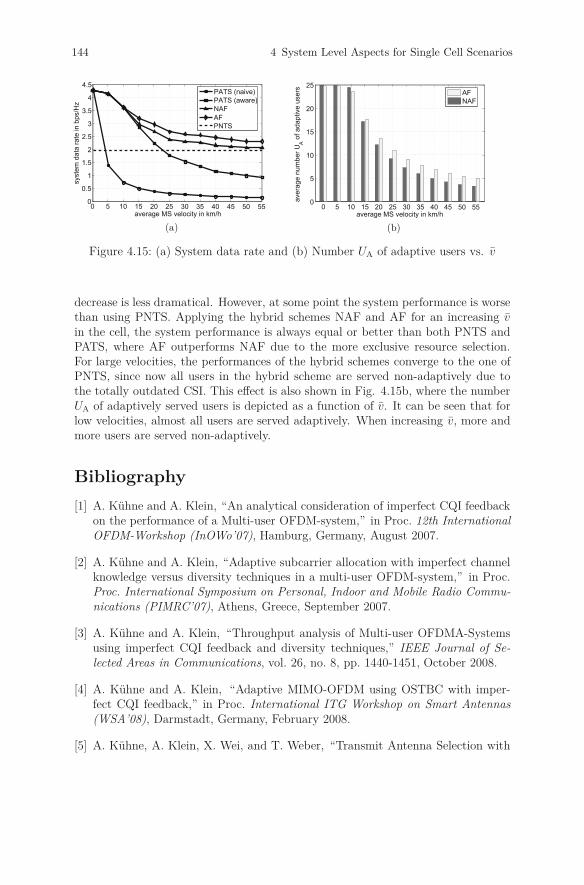
144 4 System Level Aspects for Single Cell Scenarios
0 5 10 15 20 25 30 35 40 45 50 550
0.5
1
1.5
2
2.5
3
3.5
4
4.5
average MS velocity in km/h
syst
em d
ata
rate
in b
ps/H
z
PATS (naive)PATS (aware)NAFAFPNTS
(a)
0 5 10 15 20 25 30 35 40 45 50 550
5
10
15
20
25
average MS velocity in km/h
aver
age
num
ber U
A of a
dapt
ive
user
s
AFNAF
(b)
Figure 4.15: (a) System data rate and (b) Number UA of adaptive users vs. v
decrease is less dramatical. However, at some point the system performance is worsethan using PNTS. Applying the hybrid schemes NAF and AF for an increasing vin the cell, the system performance is always equal or better than both PNTS andPATS, where AF outperforms NAF due to the more exclusive resource selection.For large velocities, the performances of the hybrid schemes converge to the one ofPNTS, since now all users in the hybrid scheme are served non-adaptively due tothe totally outdated CSI. This effect is also shown in Fig. 4.15b, where the numberUA of adaptively served users is depicted as a function of v. It can be seen that forlow velocities, almost all users are served adaptively. When increasing v, more andmore users are served non-adaptively.
Bibliography
[1] A. Kühne and A. Klein, “An analytical consideration of imperfect CQI feedbackon the performance of a Multi-user OFDM-system,” in Proc. 12th InternationalOFDM-Workshop (InOWo’07), Hamburg, Germany, August 2007.
[2] A. Kühne and A. Klein, “Adaptive subcarrier allocation with imperfect channelknowledge versus diversity techniques in a multi-user OFDM-system,” in Proc.Proc. International Symposium on Personal, Indoor and Mobile Radio Commu-nications (PIMRC’07), Athens, Greece, September 2007.
[3] A. Kühne and A. Klein, “Throughput analysis of Multi-user OFDMA-Systemsusing imperfect CQI feedback and diversity techniques,” IEEE Journal of Se-lected Areas in Communications, vol. 26, no. 8, pp. 1440-1451, October 2008.
[4] A. Kühne and A. Klein, “Adaptive MIMO-OFDM using OSTBC with imper-fect CQI feedback,” in Proc. International ITG Workshop on Smart Antennas(WSA’08), Darmstadt, Germany, February 2008.
[5] A. Kühne, A. Klein, X. Wei, and T. Weber, “Transmit Antenna Selection with

Bibliography 145
imperfect CQI feedback in Multi-user OFDMA systems,” in Proc. Proc. 13-thInternational OFDM-Workshop (InOWo’08), Hamburg, August 2008.
[6] A. Kühne and A. Klein, “Combining adaptive and non-adaptive Multi-userOFDMA schemes in the presence of user-dependent imperfect channel knowl-edge,” IEEE Transactions on Wireless Communications. (submitted)
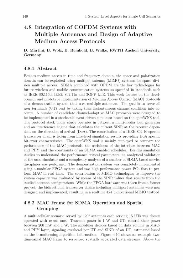
146 4 System Level Aspects for Single Cell Scenarios
4.8 Integration of COFDM Systems with
Multiple Antennas and Design of Adaptive
Medium Access Protocols
D. Martini, B. Wolz, B. Rembold, B. Walke, RWTH Aachen University,Germany
4.8.1 Abstract
Besides medium access in time and frequency domain, the space and polarizationdomain can be exploited using multiple antenna (MIMO) systems for space divi-sion multiple access. SDMA combined with OFDM are the key technologies forfuture wireless and mobile communication systems as specified in standards suchas IEEE 802.16d, IEEE 802.11n and 3GPP LTE. This work focuses on the devel-opment and prototype implementation of Medium Access Control (MAC) protocolsof a demonstration system that uses multiple antennas. The goal is to serve alluser terminals (UT) best by taking their instantaneous channel condition into ac-count. A number of candidate channel-adaptive MAC protocols were designed tobe implemented in a stochastic event driven simulator based on the openWNS tool.The protocol stack under study operates in between a multi-media load generatorand an interference engine that calculates the current SINR at the receiver depen-dent on the direction of arrival (DoA). The contribution of a IEEE 802.16 specifictransceiver chain is fed-in from link-level simulation results providing DoA specificbit-error characteristics. The openWNS tool is mainly employed to compare theperformance of the MAC protocols, the usefulness of the interface between MACand PHY and the constraints of an SDMA enabled scheduler. Besides simulationstudies to understand the performance critical parameters, an analytical validationof the used simulator and a complexity analysis of a number of SDMA based servicedisciplines was performed. The demonstration system was completely implementedusing a modular FPGA system and two high-performance power PCs that to per-form MAC in real time. The contribution of MIMO technologies to improve thesystem capacity was evaluated by means of the SINR values that results from thestudied antenna configurations. While the FPGA hardware was taken from a formerproject, the bidirectional transceiver chains including multiport antennas were newdesigned and implemented, resulting in a realtime 4x4 bidirectional MIMO testbed.
4.8.2 MAC Frame for SDMA Operation and SpatialGrouping
A multi-cellular scenario served by 120◦ antennas each serving 15 UTs was chosenoperated with re-use one. Transmit power is 1 W and UTs control their powerbetween 200 mW and 1 W. The scheduler decides based on data volume in MAC-and PHY layer, signaling overhead per UT and SINR of an UT, estimated basedon the beamforming algorithm information. Figure 4.16 shows an example two-dimensinal MAC frame to serve two spatially separated data streams. Above the

4.8 Integration of COFDM Systems 147
MAC frame the transmit situation is shown using abstract antenna diagrams. Thefirst part of the frame is transmitted omnidirectional to implement broadcast mode.DL-MAP (blue) and UL-MAP (green) and arrows are shown pointing to the timeinstants contained in the MAPs, where up to four radio bursts can be transmitted,spatially separated. Similar applies to the UL-MAP.
UTs cannot be arbitrarily scheduled for concurrent SDMA transmissions sincetheir spatial separability by the beam-forming antenna array depends on their rel-ative spatial positions. Spatially separated concurrent transmissions cannot be as-sumed to be orthogonal. Therefore, a hierarchical scheduling algorithm is introducedthat first computes a spatial grouping of UTs that can be well separated by the basestation’s (BS) beamforming antenna. The result of this grouping is a set of groupsof UTs. Users of the same spatial group can be separated and thus be served atthe same time. Users in different groups must be separated in the time domain.Structuring of the scheduling process into two hierarchical steps adds flexibility andsimplicity to the scheduling process. The grouping process is independent from theTDMA scheduling and vice versa. Thus, spatial grouping and group scheduling pro-cedures can be freely combined and interchanged according to the specific needs ofthe system. Spatial grouping of UTs has been proposed earlier [2] and hierarchicalgrouping and scheduling in an SDMA enhanced IEEE 802.16 systems is proposedfirst in [4]. Since an optimal grouping is far too complex to be applied, a greedy al-gorithm to sort spatial groups according to achievable throughput was used resultingin grouping gain slightly below the optimal grouper’s gain. A tree-based heuristicalgorithm only estimating the most promising spatial groups appear well suited toreduce run-time complexity to be applicable in real-time condition, with a groupinggain comparable to that of the greedy algorithm.
Simulation Results
Figure 4.17 shows the aggregate DL cell throughput versus offered traffic. Satura-tion is reached where the throughput deviates to grow linearly with offered traffic.Clearly, with omnidirectional it is lower than with SFIR or SDMA transmission.Under SDMA with up to 4 parallel transmissions, the throughput curve climbs froma value of about 22 MBit/s, where the first UTs reach saturation, to a final maximumof 30 MBit/s. SDMA transmission with up to 4 beams achieves about 440% gaincompared to omnidirectional transmission. Most of the results on MIMO basedMAC protocols, grouping etc. gained in this project are available from [3]. Thescheduler algorithms developed for multiple antenna systems were implemented ona real-time hardware platform.
4.8.3 Hardware Implementation of COFDM Systems with
Multiple Antennas
A realtime testbed was developed and used to validate the scheduler algorithms in“real world” scenario. The demonstrator architecture had to be adapted resulting inredesign of the analog frontend as well as the digital transceiver. The testbed is basedon OFDM transmission with 256 subcarriers for each UT. A WLAN transceiver chip
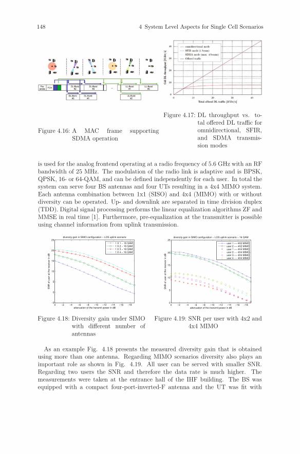
148 4 System Level Aspects for Single Cell Scenarios
Figure 4.16: A MAC frame supportingSDMA operation
Figure 4.17: DL throughput vs. to-tal offered DL traffic foromnidirectional, SFIR,and SDMA transmis-sion modes
is used for the analog frontend operating at a radio frequency of 5.6 GHz with an RFbandwidth of 25 MHz. The modulation of the radio link is adaptive and is BPSK,QPSK, 16- or 64-QAM, and can be defined independently for each user. In total thesystem can serve four BS antennas and four UTs resulting in a 4x4 MIMO system.Each antenna combination between 1x1 (SISO) and 4x4 (MIMO) with or withoutdiversity can be operated. Up- and downlink are separated in time division duplex(TDD). Digital signal processing performs the linear equalization algorithms ZF andMMSE in real time [1]. Furthermore, pre-equalization at the transmitter is possibleusing channel information from uplink transmission.
0 −2 −4 −6 −8 −10 −12 −14 −16 −18−5
0
5
10
15
20
25diversity gain in SIMO configuration − LOS uplink scenario
attenuation of the transmit power in dB
SN
R o
f user
at th
e r
eceiv
er
in d
B
1 X 1 − 16 QAM
1 X 2 − 16 QAM
1 X 3 − 16 QAM
1 X 4 − 16 QAM
Figure 4.18: Diversity gain under SIMOwith different number ofantennas
0 −2 −4 −6 −8 −10 −12 −14 −16 −180
5
10
15
20
25diversity gain in SIMO configuration − LOS uplink scenario − 16 QAM
attenuation of the transmit power in dB
SN
R o
f user
at th
e r
eceiv
er
in d
B
user 1 −− 4X2 MIMO
user 2 −− 4X2 MIMO
user 1 −− 4X4 MIMO
user 2 −− 4X4 MIMO
user 3 −− 4X4 MIMO
user 4 −− 4X4 MIMO
Figure 4.19: SNR per user with 4x2 and4x4 MIMO
As an example Fig. 4.18 presents the measured diversity gain that is obtainedusing more than one antenna. Regarding MIMO scenarios diversity also plays animportant role as shown in Fig. 4.19. All user can be served with smaller SNR.Regarding two users the SNR and therefore the data rate is much higher. Themeasurements were taken at the entrance hall of the IHF building. The BS wasequipped with a compact four-port-inverted-F antenna and the UT was fit with
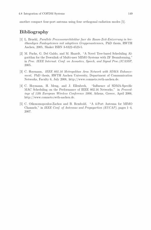
4.8 Integration of COFDM Systems 149
another compact four-port antenna using four orthogonal radiation modes [5].
Bibliography
[1] L. Bruehl, Parallele Prozessorarchitektur fuer die Raum-Zeit-Entzerrung in bre-itbandigen Funksystemen mit adaptiven Gruppenantennen, PhD thesis, RWTHAachen, 2005, Shaker ISBN 3-8322-4523-5.
[2] M. Fuchs, G. Del Galdo, and M. Haardt, “A Novel Tree-based Scheduling Al-gorithm for the Downlink of Multi-user MIMO Systems with ZF Beamforming,”in Proc. IEEE Internat. Conf. on Acoustics, Speech, and Signal Proc.(ICASSP,2005.
[3] C. Hoymann, IEEE 802.16 Metropolitan Area Network with SDMA Enhance-ment, PhD thesis, RWTH Aachen University, Department of CommunicationNetworks, Faculty 6, July 2008, http://www.comnets.rwth-aachen.de.
[4] C. Hoymann, H. Meng, and J. Ellenbeck, “Influence of SDMA-SpecificMAC Scheduling on the Performance of IEEE 802.16 Networks,” in Proceed-ings of 12th European Wireless Conference 2006, Athens, Greece, April 2006,http://www.comnets.rwth-aachen.de.
[5] C. Oikonomopoulos-Zachos and B. Rembold, “A 4-Port Antenna for MIMOChannels,” in IEEE Conf. of Antennas and Propagartion (EUCAP), pages 1–4,2007.
150 4 System Level Aspects for Single Cell Scenarios
4.9 Large System Analysis of Nearly Optimum
Low Complex Beamforming in Multicarrier
Multiuser Multiantenna Systems
C. Guthy, W. Utschick, Technische Universität München, Germany
4.9.1 Introduction
In general, analytical expressions for the average sum rate in the Multiple-InputMultiple-Output (MIMO) Broadcast Channel (BC), resulting from signal process-ing algorithms requiring perfect channel state information at the transmitter, aredifficult to obtain. That is true for the optimum sum capacity [11] as well as nearoptimum algorithms such as the Successive Encoding Successive Allocation Method(SESAM) [9] and its variant with Minimum Mean Square Error (MMSE) trans-mit filters [8, Ch. 4.2]. Thus, performance evaluation of these algorithms is onlypossible via simulation results. In the large system limit however, i.e., when atleast two system parameters go to infinity at a fixed and finite ratio [6, 10], theperformance of many algorithms becomes deterministic, although random variablesare used. That is because the eigenvalues of random matrices often converge to anasymptotic limit, which can be obtained from the asymptotic eigenvalue distribution(a.e.d.) and which is independent of the current realization of the random matrix.The most prominent example is the Marčenko-Pastur distribution [5] for Wishartmatrices. Furthermore the analytical expressions in the large system limit oftenserve as a good approximation of the system performance also with finite systemparameters, which makes large system analysis an interesting tool for the analysisof signal processing algorithms.In this chapter we will present analytical approximations of the ergodic sum ratesachievable with SESAM with MMSE transmit filters [8] and zero-forcing transmitfilters [9] based on large system results with Gaussian i.i.d. channel matrices and aninfinite number of transmit and receive antennas. It will be shown that the resultsalso serve as good approximations for the average sum rate in systems with finiteparameters.
4.9.2 System Model
We consider a multi-user multi-carrier MIMO system with C carriers, one base sta-tion with N antennas and K non-cooperative users with R antennas. The k-thuser’s channel matrix on carrier c, denoted as Hk,c ∈ CR×N , consists of uncorre-lated Gaussian entries with zero mean and variance 1/R. Perfect knowledge of thematrices Hk,c at the transmitter is assumed. The additive noise at each receiver isassumed to be white Gaussian with zero mean and unit covariance matrix.
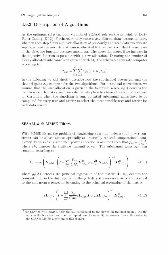
4.9 Large System Analysis 151
4.9.3 Description of Algorithms
As the optimum solution, both variants of SESAM rely on the principle of DirtyPaper Coding (DPC). Furthermore they successively allocate data streams to users,where in each step filters and user allocation of previously allocated data streams arekept fixed and the next data stream is allocated to that user such that the increasein the objective function becomes maximum. The allocation stops, if no increase inthe objective function is possible with a new allocation. Denoting the number oftotally allocated subchannels on carrier c with Mc, the achievable sum rate computesaccording to
Rsum =C∑
c=1
Mc∑i=1
log2(1 + pi,cλi,c).
In the following we will shortly describe how the subchannel powers pi,c and thechannel gains λi,c compute for the two algorithms. For notational convenience, weassume that the user allocation is given in the following, where πc(i) denotes theuser to which the data stream encoded at i-th place has been allocated to on carrierc. Certainly, when the algorithm is run, potential subchannel gains have to becomputed for every user and carrier to select the most suitable user and carrier foreach data stream.
SESAM with MMSE Filters
With MMSE filters, the problem of maximizing sum rate under a total power con-straint can be solved almost optimally at drastically reduced computational com-plexity. In this case a simplified power allocation is assumed such that pi,c = PTx
CMc
7,where PTx denotes the available transmit power. The subchannel gains λi,c thencompute according to
λi,c = ρ1
⎛⎜⎝Hπc(i),c
⎛⎝I +
i−1∑j=1
PTx
CMc
HH
πc(j),ctj,ctH
j,cHπc(j),c
⎞⎠−1
HH
πc(i),c
⎞⎟⎠ , (4.11)
where ρ1(A) denotes the principal eigenvalue of the matrix A. tj,c denotes thetransmit filter in the dual uplink for the j-th data stream on carrier c and is equalto the unit-norm eigenvector belonging to the principal eigenvalue of the matrix
Hπc(i),c
⎛⎝I +
i−1∑j=1
PTx
CMc
HH
πc(j),ctj,ctH
j,cHπc(j),c
⎞⎠−1
HH
πc(i),c (4.12)
7For SESAM with MMSE filter the pi,c correspond to the powers in the dual uplink. As therates in the broadcast and the dual uplink are the same [8], we consider the uplink rates forthe SESAM MMSE algorithm in this chapter.
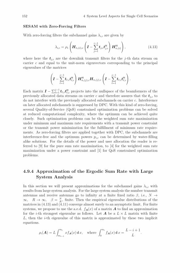
152 4 System Level Aspects for Single Cell Scenarios
SESAM with Zero-Forcing Filters
With zero-forcing filters the subchannel gains λi,c are given by
λi,c = ρ1
⎛⎝Hπc(i),c
⎛⎝I −
i−1∑j=1
tj,ctH
j,c
⎞⎠HH
πc(i)
⎞⎠ , (4.13)
where here the tj,c are the downlink transmit filters for the j-th data stream oncarrier c and equal to the unit-norm eigenvectors corresponding to the principaleigenvalues of the matrices
⎛⎝I −
j−1∑=1
t,ctH
,c
⎞⎠HH
πc(j),cHπc(j),c
⎛⎝I −
j−1∑=1
t,ctH
,c
⎞⎠ .
Each matrix I −∑j−1=1 t,ct
H
,c projects into the nullspace of the beamformers of thepreviously allocated data streams on carrier c and therefore assures that the tj,c todo not interfere with the previously allocated subchannels on carrier c. Interferenceon later allocated subchannels is suppressed by DPC. With this kind of zero-forcing,several Quality-of-Service (QoS) constrained optimization problems can be solvedat reduced computational complexity, where the optimum can be achieved quiteclosely. Such optimization problems can be the weighted sum rate maximizationunder minimum and maximum rate requirements with a transmit power constraintor the transmit power minimization for the fulfillment of minimum rate require-ments. As zero-forcing filters are applied together with DPC, the subchannels areinterference-free and the optimum powers pi,c can be determined by water-fillingalike solutions. For the details of the power and user allocation the reader is re-ferred to [9] for the pure sum rate maximization, to [4] for the weighted sum ratemaximization under a power constraint and [1] for QoS constrained optimizationproblems.
4.9.4 Approximation of the Ergodic Sum Rate with LargeSystem Analysis
In this section we will present approximations for the subchannel gains λi,c withresults from large system analysis. For the large system analysis the number transmitantennas and receive antennas go to infinity at a finite fixed ratio β, i.e., N →∞, R → ∞, β = N
R, finite. Then the empirical eigenvalue distributions of the
matrices in (4.13) and (4.11) converge almost surely to an asymptotic limit. For finitesystems, we propose to use the a.e.d. fA(x) of a matrix A to find an approximationfor the i-th strongest eigenvalue as follows. Let A be a L × L matrix with finiteL, then the i-th eigenvalue of this matrix is approximated by these two implicitequations.
ρi(A) = L∫ mi
mi−1
xfA(x) d x, where∫ mi
0fA(x) d x =
L − i + 1
L.
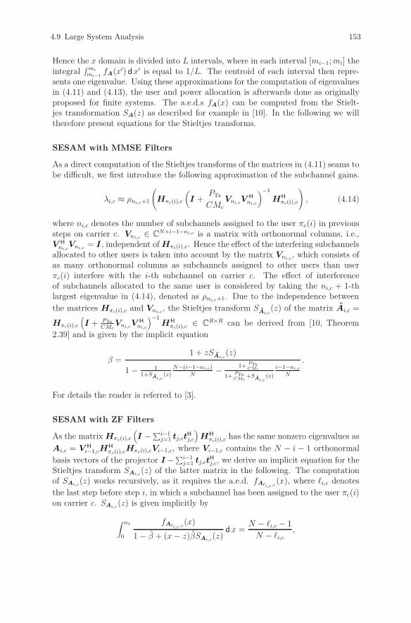
4.9 Large System Analysis 153
Hence the x domain is divided into L intervals, where in each interval [mi−1; mi] theintegral
∫mimi−1
fA(x′) d x′ is equal to 1/L. The centroid of each interval then repre-sents one eigenvalue. Using these approximations for the computation of eigenvaluesin (4.11) and (4.13), the user and power allocation is afterwards done as originallyproposed for finite systems. The a.e.d.s fA(x) can be computed from the Stielt-jes transformation SA(z) as described for example in [10]. In the following we willtherefore present equations for the Stieltjes transforms.
SESAM with MMSE Filters
As a direct computation of the Stieltjes transforms of the matrices in (4.11) seams tobe difficult, we first introduce the following approximation of the subchannel gains.
λi,c ≈ ρni,c+1
(Hπc(i),c
(I +
PTx
CMc
Vni,cVH
ni,c
)−1
HH
πc(i),c
), (4.14)
where ni,c denotes the number of subchannels assigned to the user πc(i) in previoussteps on carrier c. Vni,c ∈ CN×i−1−ni,c is a matrix with orthonormal columns, i.e.,V H
ni,cVni,c = I , independent of Hπc(i),c. Hence the effect of the interfering subchannels
allocated to other users is taken into account by the matrix Vni,c, which consists ofas many orthonormal columns as subchannels assigned to other users than userπc(i) interfere with the i-th subchannel on carrier c. The effect of interferenceof subchannels allocated to the same user is considered by taking the ni,c + 1-thlargest eigenvalue in (4.14), denoted as ρni,c+1. Due to the independence between
the matrices Hπc(i),c and Vni,c, the Stieltjes transform SAi,c(z) of the matrix Ai,c =
Hπc(i),c
(I + PTx
CMcVni,cV
H
ni,c
)−1HH
πc(i),c ∈ CR×R can be derived from [10, Theorem2.39] and is given by the implicit equation
β =1 + zSAi,c
(z)
1 − 11+S
Ai,c(z)
N−(i−1−ni,c)
N− 1+
PTxCMc
1+PTxCMc
+SAi,c
(z)
i−1−ni,c
N
.
For details the reader is referred to [3].
SESAM with ZF Filters
As the matrix Hπc(i),c
(I −∑i−1
j=1 tj,ctH
j,c
)HH
πc(i),c has the same nonzero eigenvalues as
Ai,c = V H
i−1,cHH
πc(i),cHπc(i),cVi−1,c, where Vi−1,c contains the N − i − 1 orthonormal
basis vectors of the projector I −∑i−1j=1 tj,ct
H
j,c, we derive an implicit equation for theStieltjes transform SAi,c(z) of the latter matrix in the following. The computationof SAi,c(z) works recursively, as it requires the a.e.d. fA�i,c,c
(x), where �i,c denotes
the last step before step i, in which a subchannel has been assigned to the user πc(i)on carrier c. SAi,c(z) is given implicitly by
∫ n1
0
fA�i,c,c(x)
1 − β + (x − z)βSAi,c(z)
d x =N − �i,c − 1
N − �i,c,
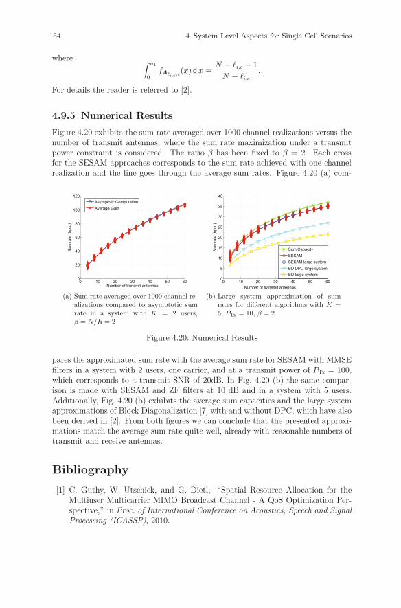
154 4 System Level Aspects for Single Cell Scenarios
where ∫ n1
0fA�i,c,c
(x) d x =N − �i,c − 1
N − �i,c
.
For details the reader is referred to [2].
4.9.5 Numerical Results
Figure 4.20 exhibits the sum rate averaged over 1000 channel realizations versus thenumber of transmit antennas, where the sum rate maximization under a transmitpower constraint is considered. The ratio β has been fixed to β = 2. Each crossfor the SESAM approaches corresponds to the sum rate achieved with one channelrealization and the line goes through the average sum rates. Figure 4.20 (a) com-
0 10 20 30 40 50 600
20
40
60
80
100
120
Number of transmit antennas
Sum
rate
(bpc
u)
Asymptotic ComputationAverage Gain
(a) Sum rate averaged over 1000 channel re-alizations compared to asymptotic sumrate in a system with K = 2 users,β = N/R = 2
0 10 20 30 40 50 600
5
10
15
20
25
30
35
40
Number of transmit antennas
Sum
rate
(bpc
u)
Sum CapacitySESAMSESAM large systemBD DPC large systemBD large system
(b) Large system approximation of sumrates for different algorithms with K =5, PTx = 10, β = 2
Figure 4.20: Numerical Results
pares the approximated sum rate with the average sum rate for SESAM with MMSEfilters in a system with 2 users, one carrier, and at a transmit power of PTx = 100,which corresponds to a transmit SNR of 20dB. In Fig. 4.20 (b) the same compar-ison is made with SESAM and ZF filters at 10 dB and in a system with 5 users.Additionally, Fig. 4.20 (b) exhibits the average sum capacities and the large systemapproximations of Block Diagonalization [7] with and without DPC, which have alsobeen derived in [2]. From both figures we can conclude that the presented approxi-mations match the average sum rate quite well, already with reasonable numbers oftransmit and receive antennas.
Bibliography
[1] C. Guthy, W. Utschick, and G. Dietl, “Spatial Resource Allocation for theMultiuser Multicarrier MIMO Broadcast Channel - A QoS Optimization Per-spective,” in Proc. of International Conference on Acoustics, Speech and SignalProcessing (ICASSP), 2010.
Bibliography 155
[2] C. Guthy, W. Utschick, and M.L. Honig, “Large System Analysis of ProjectionBased Algorithms for the MIMO Broadcast Channels,” submitted to Interna-tional Symposium on Information Theory (ISIT), 2010.
[3] C. Guthy, W. Utschick, and M.L. Honig, “Large System Analysis of the Suc-cessive Encoding Successive Allocation Method for the MIMO BC,” In Proc.of ITG/IEEE Workshop on Smart Antennas, 2010.
[4] C. Guthy, W. Utschick, R. Hunger, and M. Joham, “Efficient Weighted SumRate Maximization With Linear Precoding,” accepted for publication in IEEETransactions on Signal Processing, December 2009.
[5] V. Marčenko and L. Pastur, “Distribution of Eigenvalues for Some Sets ofRandom Matrices,” Math USSR Sbornik, 1:457–483, 1967.
[6] M.J.M. Peacock, I.B. Collings, and M.L. Honig, “Advances in Multiuser Detec-tion,” volume 1 of Wiley Series in Telecommunications and Signal Processing,chapter 4 Performance with Random Signatures. John Wiley & Sons, 2009.
[7] Q.H. Spencer, A.L. Swindlehurst, and M. Haardt, “Zero-forcing Methods forDownlink Spatial Multiplexing in Multiuser MIMO Channels,” IEEE Transac-tions on Signal Processing, 52(2):461–471, February 2004.
[8] P. Tejera, Principles and Algorithms for Transmission in Multiple-InputMultiple-Output Systems, PhD thesis, Technische Universität München, 2008.
[9] P. Tejera, W. Utschick, G. Bauch, and J. A. Nossek, “Subchannel Allocationin Multiuser Multiple Input Multiple Output Systems,” IEEE Transactions onInformation Theory, 52(10):4721–4733, October 2006.
[10] A.M. Tulino and S. Verdu, “Random Matrix Theory and Wireless Communi-cations,” Number 1 in Foundations and Trends in Communications and Infor-mation Theory. Now Publishers, 2004.
[11] H. Viswanathan, S. Venkatesan, and H. Huang, “Downlink Capacity Evaluationof Cellular Networks With Known-Interference Cancellation,” IEEE Journal onSelected Areas in Communications, 21(6):802–811, June 2003.
156 4 System Level Aspects for Single Cell Scenarios
4.10 Combined Radar and Communication
Systems Using OFDM
M. Braun, C. Sturm, F. Jondral, T. Zwick, Karlsruhe Institute of Tech-nology (KIT), Germany
4.10.1 Introduction
In the current technological development, the radio frequency front-end architecturesused in radar and digital communication technology are becoming more and moresimilar. In both applications more and more functions that have traditionally beenaccomplished by hardware components are now being replaced by digital signal pro-cessing algorithms. Moreover, today’s digital communication systems use frequenciesin the microwave regime for transmission, which are close to the frequency bandstraditionally used for radar applications. This technological advancement opens thepossibility for the implementation of joint radar and communication systems thatare able to support both applications with one single platform and even with a com-mon transmit signal. A typical application area for such systems would be intelligenttransportation networks, which require the ability for inter-vehicle communicationsas well as the need for reliable environment sensing.
First concepts of joint radar and communication systems have been primarilybased on spread spectrum techniques. Recently, OFDM signals have gained a lot ofattraction for this purpose. This is motivated by two facts: First, most currentlyreleased communications standards, e.g., IEEE 802.11p, employ OFDM signals. Sec-ond, in the radar community OFDM signals recently have attracted general interestand their suitability for radar applications has been proven. Hence, OFDM signalscurrently seem to be the ideal basis for joint radar and communication implementa-tions.
A possible application scenario of an OFDM based joint radar and communicationsystem is illustrated in Fig. 4.21. The OFDM signal (colored in green) is transmittedfrom the car on the left side and transports information to distant receivers. At thesame time this signal is reflected at objects, also cars, in the neighborhood (reflectedsignal depicted in gray). The OFDM system observes the echoes of its own transmitsignal and calculates a radar image by applying suitable processing algorithms. Also,communication with base stations could be included in this concept.
In the following, detailed considerations regarding an optimum parametrization ofthe OFDM signals for simultaneous radar and communication operation as well asoptimum radar processing strategies will be discussed. Moreover, a fully operationalsystem demonstrator and verification measurement results will be presented.
4.10.2 Signal Design
A major challenge is the design of the OFDM signals. It must be guaranteed thatthe communication link is reliable over mobile communication channels with severefading, and that the radar imaging algorithm is not negatively affected by the signal
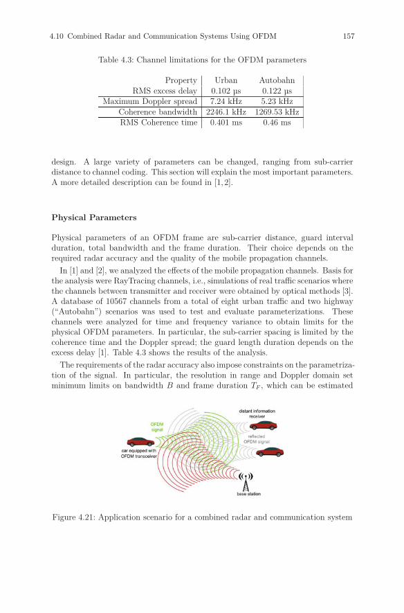
4.10 Combined Radar and Communication Systems Using OFDM 157
Table 4.3: Channel limitations for the OFDM parameters
Property Urban AutobahnRMS excess delay 0.102 μs 0.122 μs
Maximum Doppler spread 7.24 kHz 5.23 kHzCoherence bandwidth 2246.1 kHz 1269.53 kHzRMS Coherence time 0.401 ms 0.46 ms
design. A large variety of parameters can be changed, ranging from sub-carrierdistance to channel coding. This section will explain the most important parameters.A more detailed description can be found in [1, 2].
Physical Parameters
Physical parameters of an OFDM frame are sub-carrier distance, guard intervalduration, total bandwidth and the frame duration. Their choice depends on therequired radar accuracy and the quality of the mobile propagation channels.
In [1] and [2], we analyzed the effects of the mobile propagation channels. Basis forthe analysis were RayTracing channels, i.e., simulations of real traffic scenarios wherethe channels between transmitter and receiver were obtained by optical methods [3].A database of 10567 channels from a total of eight urban traffic and two highway(“Autobahn”) scenarios was used to test and evaluate parameterizations. Thesechannels were analyzed for time and frequency variance to obtain limits for thephysical OFDM parameters. In particular, the sub-carrier spacing is limited by thecoherence time and the Doppler spread; the guard length duration depends on theexcess delay [1]. Table 4.3 shows the results of the analysis.
The requirements of the radar accuracy also impose constraints on the parametriza-tion of the signal. In particular, the resolution in range and Doppler domain setminimum limits on bandwidth B and frame duration TF , which can be estimated
Figure 4.21: Application scenario for a combined radar and communication system
158 4 System Level Aspects for Single Cell Scenarios
by the following equations:
B ≥ c0
2Δdmax
, TF ≥ c0
2Δvmaxfc
(4.15)
For a range resolution of 1.5 m, the bandwidth must therefore be on the order of100 MHz. This in turn has other side effects, such as a low power density.
A less obvious design criterion is the effect of the parametrization on the OFDMradar processing algorithm. The maximum likelihood estimator presented in thefollowing section is prone to threshold effects. In [4], we present a method to testthe range in which a given set of parameters works without threshold effects.
Channel Coding
A suitable channel coding is an important choice in the frame design process. Ve-hicular applications in particular have high demands regarding reliability of thedata transmission. At the same time, the signal’s low power density and the highlyfrequency- and time-variant channels make error-free data transmission very diffi-cult. On the other hand, the large bandwidth allows for high data rates, whichmight not be necessary. It therefore makes sense to sacrifice raw data rate for lowerbit error rates by using robust codes with low coding rates.
Although several types of codes can satisfy these requirements, Reed-Muller codesappear particularly suitable. Their big advantage is the possibility to use sub-sets ofcodes which exhibit a low peak-to-average power ratio (PAPR) [5, 6]. This is givesthe whole system a new degree of freedom, since the low PAPR values exhibit fewerrequirements towards the amplifiers. Simulations have shown the codes to performwell under adverse channel effects with a fixed PAPR of 3 dB [5].
4.10.3 The Radar Subsystem
The radar subsystem deals with the task of estimating range and relative speedof other objects in the vicinity. When transmitting, it receives and analyses thebackscattered signal and processes it to gain information about the surroundingobjects. In order to identify a suitable estimation algorithm we must first analyzethe effects the backscattering has on OFDM frames.
In the following, one OFDM frame shall be described by an N × M-matrix FTx ∈CN×M , where every element (FTx)k,l) = ±1 is a modulation symbol from the BPSKmodulation alphabet. Every row in FTx corresponds to an OFDM sub-carrier; everycolumn corresponds to an OFDM symbol. s(t) denotes the transmitted time domainsignal and is created from FTx by the usual OFDM modulation process of calculatingan IFFT of every column and prepending the result with a cyclic prefix.
During transmission, a receiver is active. The received signal r(t) consists ofthe Doppler shifted and time-delayed reflected signals. In the case of H reflectingtargets, the relation between transmitted and received signals is
r(t) =H−1∑h=0
bhs(t − τh)ej2πfD,ht + wσ2(t). (4.16)
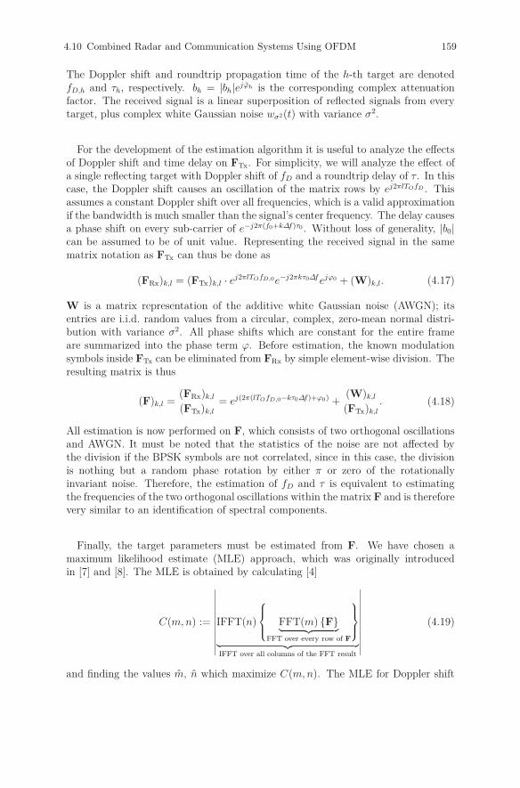
4.10 Combined Radar and Communication Systems Using OFDM 159
The Doppler shift and roundtrip propagation time of the h-th target are denotedfD,h and τh, respectively. bh = |bh|ejϕh is the corresponding complex attenuationfactor. The received signal is a linear superposition of reflected signals from everytarget, plus complex white Gaussian noise wσ2(t) with variance σ2.
For the development of the estimation algorithm it is useful to analyze the effectsof Doppler shift and time delay on FTx. For simplicity, we will analyze the effect ofa single reflecting target with Doppler shift of fD and a roundtrip delay of τ . In thiscase, the Doppler shift causes an oscillation of the matrix rows by ej2πlTOfD . Thisassumes a constant Doppler shift over all frequencies, which is a valid approximationif the bandwidth is much smaller than the signal’s center frequency. The delay causesa phase shift on every sub-carrier of e−j2π(f0+kΔf)τ0 . Without loss of generality, |b0|can be assumed to be of unit value. Representing the received signal in the samematrix notation as FTx can thus be done as
(FRx)k,l = (FTx)k,l · ej2πlTOfD,0e−j2πkτ0Δf ejϕ0 + (W)k,l. (4.17)
W is a matrix representation of the additive white Gaussian noise (AWGN); itsentries are i.i.d. random values from a circular, complex, zero-mean normal distri-bution with variance σ2. All phase shifts which are constant for the entire frameare summarized into the phase term ϕ. Before estimation, the known modulationsymbols inside FTx can be eliminated from FRx by simple element-wise division. Theresulting matrix is thus
(F)k,l =(FRx)k,l
(FTx)k,l
= ej(2π(lTOfD,0−kτ0Δf)+ϕ0) +(W)k,l
(FTx)k,l
. (4.18)
All estimation is now performed on F, which consists of two orthogonal oscillationsand AWGN. It must be noted that the statistics of the noise are not affected bythe division if the BPSK symbols are not correlated, since in this case, the divisionis nothing but a random phase rotation by either π or zero of the rotationallyinvariant noise. Therefore, the estimation of fD and τ is equivalent to estimatingthe frequencies of the two orthogonal oscillations within the matrix F and is thereforevery similar to an identification of spectral components.
Finally, the target parameters must be estimated from F. We have chosen amaximum likelihood estimate (MLE) approach, which was originally introducedin [7] and [8]. The MLE is obtained by calculating [4]
C(m, n) :=
∣∣∣∣∣∣∣∣∣∣∣∣IFFT(n)
⎧⎪⎨⎪⎩ FFT(m) {F}︸ ︷︷ ︸
FFT over every row of F
⎫⎪⎬⎪⎭
︸ ︷︷ ︸IFFT over all columns of the FFT result
∣∣∣∣∣∣∣∣∣∣∣∣(4.19)
and finding the values m, n which maximize C(m, n). The MLE for Doppler shift

160 4 System Level Aspects for Single Cell Scenarios
and propagation time is then
τ =n
NIFFTΔf, fD =
m
MFFTTO
, (4.20)
where NIFFT and MFFT are the lengths of the IFFT and the FFT, respectively. Itmust be noted that the complexity of such an approach is smaller than the classicalapproach of correlating in frequency and time domain. Moreover, additional inves-tigations have been conducted regarding the estimation of the direction of arrival(DoA) with a multiple antenna receiver. It has been shown that standard DoA es-timation techniques can be applied directly to the output of the range and velocityestimators in Eq. (6). Detailed results have been published in [9].
4.10.4 Measurements
Demonstrator Setup
The demonstrator system consists of three main hardware components: a Rohde &Schwarz (R&S) SMJ100A vector signal generator, a R&S FSQ26 signal analyzer,and optionally a R&S SMR40 microwave signal generator. The SMJ100A is limitedto a maximum carrier frequency of 6 GHz but offers higher output power than theSMR40. Therefore it has been decided to implement two different configurations,one with the SMJ100A only in order to achieve high output power at 6 GHz andanother one with both SMJ100A and SMR40 in order to generate a signal at theintended carrier frequency of 24 GHz but with reduced transmit power. All instru-ments are connected through an Ethernet link and controlled from a computer viathe MatLab Instrument Control Toolbox. All signals are generated and processedin MatLab. The OFDM system parameters that have been applied for the measure-ments are summarized in Table 4.4. These parameters have been obtained througha theoretical study described in [10] and verified with ray tracing simulations in [1].
Table 4.4: OFDM system parameters
Symbol Quantity Value
fc Carrier frequency 6 GHz / 24 GHzNc Number of subcarriers 1024Δf Subcarrier spacing 90.909 kHzT Elementary OFDM symbol duration 11 μsTp Cyclic prefix length 1.375 μsB Total signal bandwidth 93.1 MHz
The first configuration of the system setup is shown in Fig. 4.22. The transmitsignal is generated in MatLab, transferred to the signal generator, converted tothe carrier frequency and radiated. The signal analyzer is synchronized in phasethrough a 10 MHz reference signal and in time through a trigger signal. The signalanalyzer samples the I and Q components of the received signal after conversion
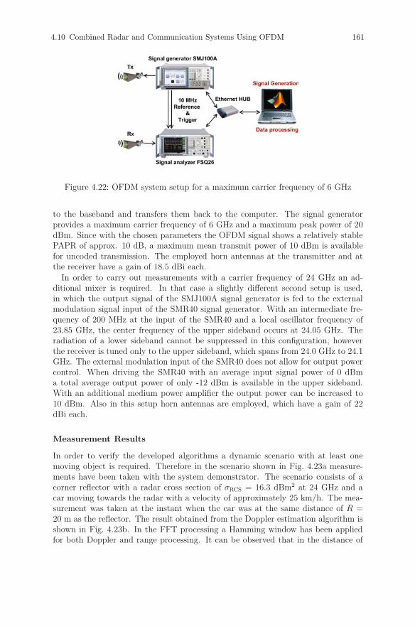
4.10 Combined Radar and Communication Systems Using OFDM 161
Figure 4.22: OFDM system setup for a maximum carrier frequency of 6 GHz
to the baseband and transfers them back to the computer. The signal generatorprovides a maximum carrier frequency of 6 GHz and a maximum peak power of 20dBm. Since with the chosen parameters the OFDM signal shows a relatively stablePAPR of approx. 10 dB, a maximum mean transmit power of 10 dBm is availablefor uncoded transmission. The employed horn antennas at the transmitter and atthe receiver have a gain of 18.5 dBi each.
In order to carry out measurements with a carrier frequency of 24 GHz an ad-ditional mixer is required. In that case a slightly different second setup is used,in which the output signal of the SMJ100A signal generator is fed to the externalmodulation signal input of the SMR40 signal generator. With an intermediate fre-quency of 200 MHz at the input of the SMR40 and a local oscillator frequency of23.85 GHz, the center frequency of the upper sideband occurs at 24.05 GHz. Theradiation of a lower sideband cannot be suppressed in this configuration, howeverthe receiver is tuned only to the upper sideband, which spans from 24.0 GHz to 24.1GHz. The external modulation input of the SMR40 does not allow for output powercontrol. When driving the SMR40 with an average input signal power of 0 dBma total average output power of only -12 dBm is available in the upper sideband.With an additional medium power amplifier the output power can be increased to10 dBm. Also in this setup horn antennas are employed, which have a gain of 22dBi each.
Measurement Results
In order to verify the developed algorithms a dynamic scenario with at least onemoving object is required. Therefore in the scenario shown in Fig. 4.23a measure-ments have been taken with the system demonstrator. The scenario consists of acorner reflector with a radar cross section of σRCS = 16.3 dBm2 at 24 GHz and acar moving towards the radar with a velocity of approximately 25 km/h. The mea-surement was taken at the instant when the car was at the same distance of R =20 m as the reflector. The result obtained from the Doppler estimation algorithm isshown in Fig. 4.23b. In the FFT processing a Hamming window has been appliedfor both Doppler and range processing. It can be observed that in the distance of
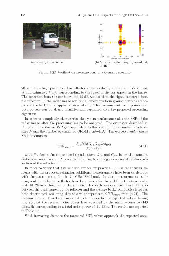
162 4 System Level Aspects for Single Cell Scenarios
(a) Investigated scenario (b) Measured radar image (normalized,in dB)
Figure 4.23: Verification measurement in a dynamic scenario
20 m both a high peak from the reflector at zero velocity and an additional peakat approximately 7 m/s corresponding to the speed of the car appear in the image.The reflection from the car is around 15 dB weaker than the signal scattered fromthe reflector. In the radar image additional reflections from ground clutter and ob-jects in the background appear at zero velocity. The measurement result proves thatboth objects can be clearly identified and separated with the proposed processingalgorithm.
In order to completely characterize the system performance also the SNR of theradar image after the processing has to be analyzed. The estimator described inEq. (4.20) provides an SNR gain equivalent to the product of the number of subcar-riers N and the number of evaluated OFDM symbols M . The expected radar imageSNR amounts to
SNRimage =PT xNMGT xGRxλ2σRCS
PN(4π3)r4(4.21)
with PT x being the transmitted signal power, GT x and GRx being the transmitand receive antenna gain, λ being the wavelength, and σRCS denoting the radar crosssection of the reflector.
In order to verify that this relation applies for practical OFDM radar measure-ments with the proposed estimator, additional measurements have been carried outwith the system setup for the 24 GHz ISM band. In these measurements radarimages of the trihedral reflector have been taken for three different distances of r= 4, 10, 20 m without using the amplifier. For each measurement result the ratiobetween the peak caused by the reflector and the average background noise level hasbeen determined, assuming that this value represents SNRimage from (4.21). Themeasured values have been compared to the theoretically expected values, takinginto account the receiver noise power level specified by the manufacturer to -143dBm/Hz corresponding to a total noise power of -64 dBm. The results are reportedin Table 4.5.
With increasing distance the measured SNR values approach the expected ones.
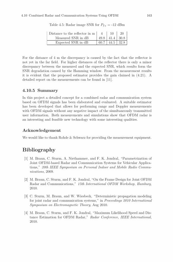
4.10 Combined Radar and Communication Systems Using OFDM 163
Table 4.5: Radar image SNR for PT x = -12 dBm
Distance to the reflector in m 4 10 20Measured SNR in dB 49.8 41.4 30.8Expected SNR in dB 60.7 44.5 32.8
For the distance of 4 m the discrepancy is caused by the fact that the reflector isnot yet in the far field. For higher distances of the reflector there is only a minordiscrepancy between the measured and the expected SNR, which results form theSNR degradation caused by the Hamming window. From the measurement resultsit is evident that the proposed estimator provides the gain claimed in (4.21). Adetailed report on the measurements can be found in [11].
4.10.5 Summary
In this project a detailed concept for a combined radar and communication systembased on OFDM signals has been elaborated and evaluated. A suitable estimatorhas been developed that allows for performing range and Doppler measurementswith OFDM signals without any negative impact of the simultaneously transmitteduser information. Both measurements and simulations show that OFDM radar isan interesting and feasible new technology with some interesting qualities.
Acknowledgement
We would like to thank Rohde & Schwarz for providing the measurement equipment.
Bibliography
[1] M. Braun, C. Sturm, A. Niethammer, and F. K. Jondral, “Parametrization ofJoint OFDM-based Radar and Communication Systems for Vehicular Applica-tions,” 20th IEEE Symposium on Personal Indoor and Mobile Radio Commu-nications, 2009.
[2] M. Braun, C. Sturm, and F. K. Jondral, “On the Frame Design for Joint OFDMRadar and Communications,” 15th International OFDM Workshop, Hamburg,2010.
[3] C. Sturm, M. Braun, and W. Wiesbeck, “Deterministic propagation modelingfor joint radar and communication systems,” in Proceedings 2010 InternationalSymposium on Electromagnetic Theory, Aug 2010.
[4] M. Braun, C. Sturm, and F. K. Jondral, “Maximum Likelihood Speed and Dis-tance Estimation for OFDM Radar,” Radar Conference, IEEE International,2010.
164 4 System Level Aspects for Single Cell Scenarios
[5] M. Braun, Y. Koch, C. Sturm, and F. K. Jondral, “Signal Design and Coding forHigh-Bandwidth OFDM in Car-to-Car Communications,” Vehicular TechnologyConference, 2010. 72nd IEEE, September 2010.
[6] J. A. Davis and J. Jedwab, “Peak-to-mean power control in OFDM, Golaycomplementary sequences and Reed-Muller codes,” IEEE Transactions on In-formation Theory, 45(7), November 1999.
[7] C. Sturm, E. Pancera, T. Zwick, and W. Wiesbeck, “A Novel Approach toOFDM Radar Processing,” Radar Conference, IEEE, May 2009.
[8] C. Sturm, M. Braun, T. Zwick, and W. Wiesbeck, “A Multiple Target DopplerEstimation Algorithm for OFDM based Intelligent Radar Systems,” 7th Euro-pean Radar Conference, 2010.
[9] C. Sturm, L. Reichardt, T. Zwick, and W. Wiesbeck, “Evaluation of beam-forming algorithms for automotive OFDM signal based radar,” in Proceedingsof the European Radar Conference EuRAD 2009, pages 141–144, Rome, Sept2009. 2009.09.30.
[10] C. Sturm, T. Zwick, and W. Wiesbeck, “An OFDM System Concept for JointRadar and Communications Operations,” Vehicular Technology Conference,2009. 69th IEEE, April 2009.
[11] C. Sturm, M. Braun, T. Zwick, and W. Wiesbeck, “Performance Verificationof Symbol-Based OFDM Radar Processing,” Radar Conference, IEEE Inter-national, 2010.
H. Rohling (ed.), OFDM: Concepts for Future Communication Systems, 165Signals and Communication Technology, DOI: 10.1007/978-3-642-17496-4_5,© Springer-Verlag Berlin Heidelberg 2011
5 System Level Aspects forMultiple Cell Scenarios
5.1 Link Adaptation
R. Kays, O. Hoffmann, TU Dortmund University, Germany
5.1.1 Motivation
OFDM based systems provide many options and parameters to set up an efficientradio transmission for given requirements and channel conditions. System designis very demanding especially if many transmissions share a limited bandwidth andhave to be optimized without a central coordination instance. Self-organizing net-works are an example for such demanding system design tasks. Especially if highrequirements on quality of service are given in an environment with many activetransmission nodes, only careful selection of link adaptation methods can yield therequired performance. In any case, the basic OFDM design has to be suited tothe transmission task. System design is based on the selection of general parame-ters like transmission frequency, bandwidth per channel, maximum transmit power(typically limited by regulation) as well as the definition of the fundamental OFDMparameters like number of carriers and the duration of the guard interval. In orderto specify a practical system, further specifications are needed to allow for synchro-nization. Transmission standards therefore include the definition of pilot carriersand synchronization symbols. Link adaptation means the dynamic choice of indi-vidual link parameters within a given OFDM-framework. Typically, this processhas to be based on the observation of the transmission conditions which influencea single radio link as well as a complete network. As the question of optimum linkadaptation is closely related to the environment of the links, many different optionsexist. In order to restrict our discussion to a limited complexity, we will focus on acertain application scenario which includes many aspects of general interest. Thisscenario is sketched in the following chapter.
5.1.2 Example of a Multiple Link Scenario
For the purpose of discussing different aspects of link adaptation, a scenario shouldbe selected which poses demanding requirements on transmission efficiency and qual-ity of service. The transmission of live media streams in home environments mayserve as such an example. Home environments are as individual as people are, andthey will differ between regions and cultures. Assuming a typical household in many

166 5 System Level Aspects for Multiple Cell Scenarios
industrial countries one might assume that a critical network situation is the simul-taneous use of different video services by several members of the household. Theremay be different local storage servers containing audio-video (AV) material boughtby the consumer (like DVD or CD collections), recorded (broadcast time shift),downloaded or produced (like personal video and still images). Furthermore, differ-ent access points to external networks are available - satellite reception equipment,broadband coax cable or twisted pair cable carrying speech communication as wellas DSL Internet access. Different devices may also link to terrestrial mobile com-munication (GSM, UMTS) or digital broadcast networks like DVB-T, DVB-H, orDAB. Figure 5.1 shows a typical scenario. Network access devices and local storageservers are located in different rooms, and manifold AV devices are used in severalplaces. Services are provided based on individual links between data sources andmedia renderers. The system has to assure that every user has convenient accessto every service - the vision of anything, anywhere, anytime should become realityfor the personal environment of people. From the system design point of view, anefficient network is required, allowing for data rates in the order of 5 - 15 Mbit/sper media stream. Although the network should appear as one logical instance fromthe users’ perspective, it consists of a number of independent links with individ-ual transmission parameters. Each link is competing for the scarce transmissionresources.
Home Office
Sat-Receiver
Kid’s Room
Living Room Kitchen
DVD/VCR
Receiver
DSL AccessPoint
PC
PC
Server
Figure 5.1: Typical wireless network in a detached house
Optimization can start by selection of suitable parameters for each individual link.The task becomes more demanding if several links are operated in parallel. It can beexpected that such network concepts will be introduced to many households. Thisfact makes the competition for scarce resources more demanding, because a limitednumber of wireless channels has to be shared between neighboring logical networks.
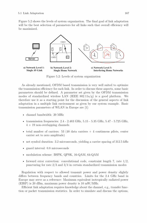
5.1 Link Adaptation 167
Figure 5.2 shows the levels of system organization. The final goal of link adaptationwill be the best selection of parameters for all links such that overall efficiency willbe maximized.
ServerServer 2
Server 1
a) Network Level 1:Single AV-Link
b) Network Level 2:Single Home Network
c) Network Level 3:Interfering Home Networks
Figure 5.2: Levels of system organization
As already mentioned, OFDM based transmission is very well suited to optimizethe transmission efficiency for each link. In order to discuss these aspects, some basicparameters should be defined. A parameter set given by the OFDM transmissionmodes of standardized wireless LAN (IEEE 802.11a/g) is a good platform. Wetherefore use it as a starting point for the discussion of the general aspects of linkadaptation in a multiple link environment as given by our system example. Basictransmission parameters of WLAN in Europe are [1]:
• channel bandwidth: 20 MHz
• transmission frequencies: 2.4 - 2.483 GHz, 5.15 - 5.35 GHz, 5.47 - 5.725 GHz,4 + 19 non-overlapping channels
• total number of carriers: 53 (48 data carriers + 4 continuous pilots, centercarrier set to zero amplitude)
• net symbol duration: 3.2 microseconds, yielding a carrier spacing of 312.5 kHz
• guard interval: 0.8 microseconds
• modulation scheme: BSPK, QPSK, 16-QAM, 64-QAM
• forward error correction: convolutional code, constraint length 7, rate 1/2,puncturing for rate 2/3 and 3/4 in certain standardized transmission modes
Regulation with respect to allowed transmit power and power density slightlydiffers between frequency bands and countries. Limits for the 2.4 GHz band inEurope may serve as a reference: Maximum equivalent isotropically radiated power(EIRP) is 20 dBm, maximum power density is 10 mW/MHz.
Efficient link adaptation requires knowledge about the channel, e.g., transfer func-tion or packet transmission statistics. In order to simulate and discuss the options,

168 5 System Level Aspects for Multiple Cell Scenarios
5.725
-80
-75
-70
-65
-60
-855.745 5.765 5.805 5.8255.785
|H(f
)|
(dB
)
frequency (GHz)
5.725
-79
-77
-75
-73
-71
-815.745 5.765 5.805 5.8255.785
|H(f
)|
(dB
)
frequency (GHz)
2.4
-77
-75
-73
-71
-69
-792.42 2.44 2.48 2.52.46
|H(f
)|
(dB
)
frequency (GHz)2.4
-62
-58
-54
-50
-46
-662.42 2.44 2.48 2.52.46
|H(f
)|
(dB
)
frequency (GHz)
Figure 5.3: Typical transfer functions in a home environment (non-line-of-sight) forthe 2.4 and 5 GHz bands, respectively. One WLAN transmission channelis a 20 MHz portion of the spectrum.

5.1 Link Adaptation 169
a channel model is required to deliver the required information. In our scenario,the coherence bandwidth is large compared to the carrier spacing. Furthermore,we assume precise channel estimation due to the pilot carriers and synchronizationsequences in WLAN. Therefore, it will be sufficient to know the amplitude transferfunction of typical transmission channels in home environments. Indoor transmissionhas been analyzed in many publications. However, most of these channel measure-ments relate to office environments. Therefore, a large number of channel transferfunction measurements in typical homes have been carried out within the scope ofthis analysis [2]. Figure 5.3 gives examples of typical transfer functions. These havebeen measured using a channel sounder which provided a radio signal of 100 MHzbandwidth. Measurements have been taken for the ISM bands at 2.4 GHz and5.75 GHz. One WLAN channel covers a portion of 20 MHz of these bands. Theresults of the measurements will be used within the following chapters.
5.1.3 Adaptation of Physical Link Parameters
Assuming the basic parameter set of IEEE 802.11a/g, the options for link adaptationon the physical layer are discussed in the following. We start the discussion for onesingle link, thus neglecting aspects of cross-layer optimization and interference withcompeting transmissions for the moment. If channel bandwidth, duration of guardinterval, number of carriers, and carrier spacing are fixed according to the standard,link adaptation in the physical layer means individual, dynamic selection of thefollowing parameters:
1. transmission channel (within the number of available channels)
2. total transmit power
3. modulation and coding scheme (and thus the physical data rate)
4. transmit power/modulation per carrier
Some of these options can be used within the boundaries of existing standards,others require extensions.
1. Dynamic Frequency Selection
In off-the-shelf WLAN products, the transmission frequency is selected once(e.g., by default parameters coming with the product or during setup proce-dure by manual selection). A dynamic selection of the transmission frequency,adapted to the transmission environment, can improve the system performancesignificantly. Selecting a channel with an advantageous transmission function(low attenuation) allows the maximization of received power and thus SNR. Ina network with high node density, the amount of competing transmissions inthe radio channels has to be taken into consideration, too. By measuring theoccupation of the channel, a second criterion for the dynamic selection of thechannel is given. Let us first consider the transmission function. Generally, thepotential for improvements depends on the scenario. In a home environment,
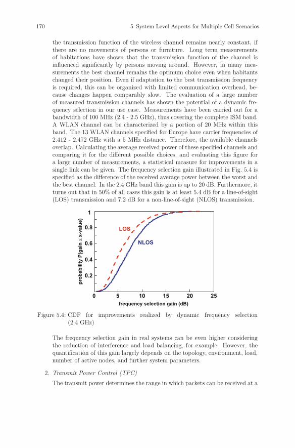
170 5 System Level Aspects for Multiple Cell Scenarios
the transmission function of the wireless channel remains nearly constant, ifthere are no movements of persons or furniture. Long term measurementsof habitations have shown that the transmission function of the channel isinfluenced significantly by persons moving around. However, in many mea-surements the best channel remains the optimum choice even when habitantschanged their position. Even if adaptation to the best transmission frequencyis required, this can be organized with limited communication overhead, be-cause changes happen comparably slow. The evaluation of a large numberof measured transmission channels has shown the potential of a dynamic fre-quency selection in our use case. Measurements have been carried out for abandwidth of 100 MHz (2.4 - 2.5 GHz), thus covering the complete ISM band.A WLAN channel can be characterized by a portion of 20 MHz within thisband. The 13 WLAN channels specified for Europe have carrier frequencies of2.412 - 2.472 GHz with a 5 MHz distance. Therefore, the available channelsoverlap. Calculating the average received power of these specified channels andcomparing it for the different possible choices, and evaluating this figure fora large number of measurements, a statistical measure for improvements in asingle link can be given. The frequency selection gain illustrated in Fig. 5.4 isspecified as the difference of the received average power between the worst andthe best channel. In the 2.4 GHz band this gain is up to 20 dB. Furthermore, itturns out that in 50% of all cases this gain is at least 5.4 dB for a line-of-sight(LOS) transmission and 7.2 dB for a non-line-of-sight (NLOS) transmission.
0 5 10 15 20 25
0.2
0.4
0.6
0.8
1
frequency selection gain (dB)
LOS
NLOS
pro
ba
bil
ity
P(g
ain
x-v
alu
e)
�
Figure 5.4: CDF for improvements realized by dynamic frequency selection(2.4 GHz)
The frequency selection gain in real systems can be even higher consideringthe reduction of interference and load balancing, for example. However, thequantification of this gain largely depends on the topology, environment, load,number of active nodes, and further system parameters.
2. Transmit Power Control (TPC)
The transmit power determines the range in which packets can be received at a
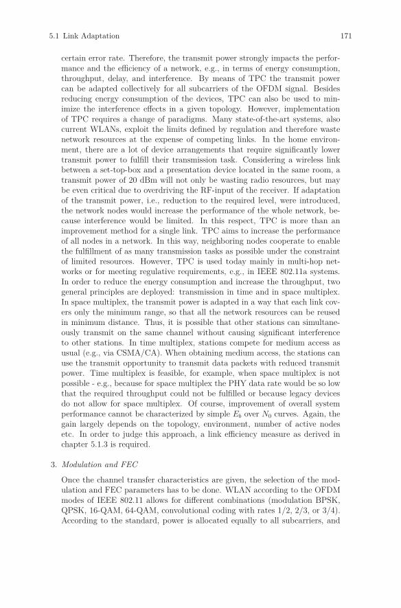
5.1 Link Adaptation 171
certain error rate. Therefore, the transmit power strongly impacts the perfor-mance and the efficiency of a network, e.g., in terms of energy consumption,throughput, delay, and interference. By means of TPC the transmit powercan be adapted collectively for all subcarriers of the OFDM signal. Besidesreducing energy consumption of the devices, TPC can also be used to min-imize the interference effects in a given topology. However, implementationof TPC requires a change of paradigms. Many state-of-the-art systems, alsocurrent WLANs, exploit the limits defined by regulation and therefore wastenetwork resources at the expense of competing links. In the home environ-ment, there are a lot of device arrangements that require significantly lowertransmit power to fulfill their transmission task. Considering a wireless linkbetween a set-top-box and a presentation device located in the same room, atransmit power of 20 dBm will not only be wasting radio resources, but maybe even critical due to overdriving the RF-input of the receiver. If adaptationof the transmit power, i.e., reduction to the required level, were introduced,the network nodes would increase the performance of the whole network, be-cause interference would be limited. In this respect, TPC is more than animprovement method for a single link. TPC aims to increase the performanceof all nodes in a network. In this way, neighboring nodes cooperate to enablethe fulfillment of as many transmission tasks as possible under the constraintof limited resources. However, TPC is used today mainly in multi-hop net-works or for meeting regulative requirements, e.g., in IEEE 802.11a systems.In order to reduce the energy consumption and increase the throughput, twogeneral principles are deployed: transmission in time and in space multiplex.In space multiplex, the transmit power is adapted in a way that each link cov-ers only the minimum range, so that all the network resources can be reusedin minimum distance. Thus, it is possible that other stations can simultane-ously transmit on the same channel without causing significant interferenceto other stations. In time multiplex, stations compete for medium access asusual (e.g., via CSMA/CA). When obtaining medium access, the stations canuse the transmit opportunity to transmit data packets with reduced transmitpower. Time multiplex is feasible, for example, when space multiplex is notpossible - e.g., because for space multiplex the PHY data rate would be so lowthat the required throughput could not be fulfilled or because legacy devicesdo not allow for space multiplex. Of course, improvement of overall systemperformance cannot be characterized by simple Eb over N0 curves. Again, thegain largely depends on the topology, environment, number of active nodesetc. In order to judge this approach, a link efficiency measure as derived inchapter 5.1.3 is required.
3. Modulation and FEC
Once the channel transfer characteristics are given, the selection of the mod-ulation and FEC parameters has to be done. WLAN according to the OFDMmodes of IEEE 802.11 allows for different combinations (modulation BPSK,QPSK, 16-QAM, 64-QAM, convolutional coding with rates 1/2, 2/3, or 3/4).According to the standard, power is allocated equally to all subcarriers, and
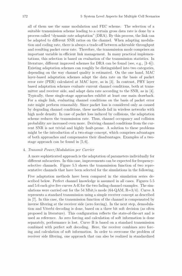
172 5 System Level Aspects for Multiple Cell Scenarios
all of them use the same modulation and FEC scheme. The selection of asuitable transmission scheme leading to a certain gross data rate is done by aprocess called “dynamic rate adaptation” (DRA). By this process, the link canbe adapted to different SNR ratios on the channel. When adapting modula-tion and coding rate, there is always a trade-off between achievable throughputand resulting packet error rate. Therefore, the transmission mode comprises animportant variable in efficient link management. In many practical implemen-tations, this selection is based on evaluation of the transmission statistics. Inliterature, different improved schemes for DRA can be found (see, e.g., [3–6]).Existing adaptation schemes can roughly be distinguished into two categories,depending on the way channel quality is estimated. On the one hand, MAClayer-based adaptation schemes adapt the data rate on the basis of packeterror rate (PER) calculated at MAC layer, as in [3]. In contrast, PHY layerbased adaptation schemes evaluate current channel conditions, both at trans-mitter and receiver side, and adapt data rate according to the SNR, as in [4].Typically, these single-stage approaches exhibit at least one main drawback.For a single link, evaluating channel conditions on the basis of packet errorrate might perform reasonably. Since packet loss is considered only as causedby degrading channel conditions, these methods fail in wireless networks withhigh node density. In case of packet loss induced by collisions, the adaptationscheme reduces the transmission rate. Thus, channel occupancy and collisionprobability are increased even more. Deriving channel conditions from the cur-rent SNR is not trivial and highly fault-prone. A solution to these problemsmight be the introduction of a two-stage concept, which comprises advantagesof both approaches and compensates their disadvantages. Examples of a two-stage approach can be found in [5, 6].
4. Transmit Power/Modulation per Carrier
A more sophisticated approach is the adaptation of parameters individually fordifferent subcarriers. In this case, improvements can be expected for frequency-selective channels. Figure 5.5 shows the transmission function of two repre-sentative channels that have been selected for the simulations in the following.
Five adaptation methods have been compared in the simulation series de-scribed below. Perfect channel knowledge is assumed in all cases. Figures 5.5and 5.6 each give five curves A-E for the two fading channel examples. The sim-ulations were carried out for the 54 Mbit/s mode (64-QAM, R=3/4). Curve Arepresents a standard transmission using a simple receiver concept as describedin [7]. In this case, the transmission function of the channel is compensated byinverse filtering at the receiver side (zero forcing). In the next step, demodula-tion and Viterbi decoding is done, based on a three bit soft decision (as oftenproposed in literature). This configuration reflects the state-of-the-art and isused as reference. As zero forcing and calculation of soft information is doneseparately, performance is lost. Curve B is based on a standard transmissioncombined with perfect soft decoding. Here, the receiver combines zero forc-ing and calculation of soft information. In order to overcome the problem ofreceiver side filtering, one approach that can also be realized in standardized
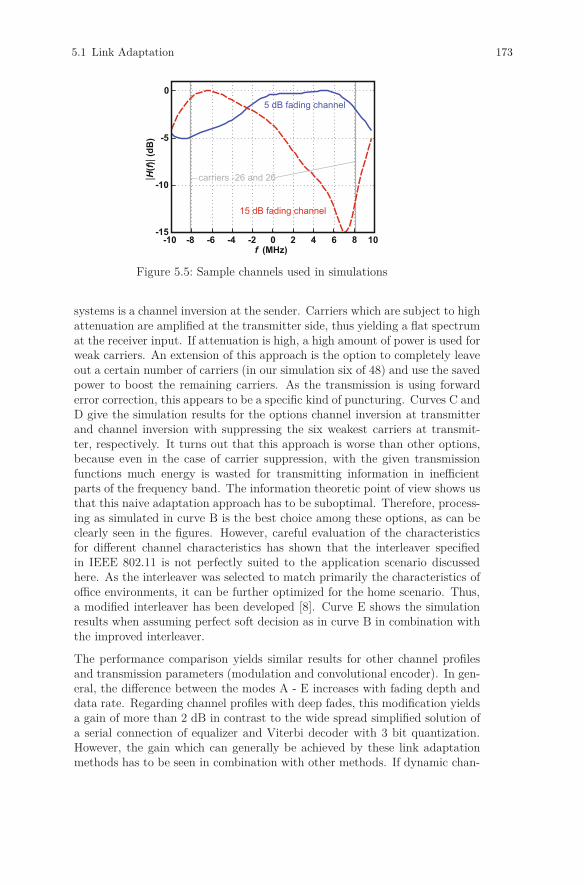
5.1 Link Adaptation 173
-15
-10
-5
0
15 dB fading channel
5 dB fading channel
carriers -26 and 26
-10 -8 -6 -4 -2 0 2 4 6 8 10(MHz)f
||
Hf()
(dB
)
Figure 5.5: Sample channels used in simulations
systems is a channel inversion at the sender. Carriers which are subject to highattenuation are amplified at the transmitter side, thus yielding a flat spectrumat the receiver input. If attenuation is high, a high amount of power is used forweak carriers. An extension of this approach is the option to completely leaveout a certain number of carriers (in our simulation six of 48) and use the savedpower to boost the remaining carriers. As the transmission is using forwarderror correction, this appears to be a specific kind of puncturing. Curves C andD give the simulation results for the options channel inversion at transmitterand channel inversion with suppressing the six weakest carriers at transmit-ter, respectively. It turns out that this approach is worse than other options,because even in the case of carrier suppression, with the given transmissionfunctions much energy is wasted for transmitting information in inefficientparts of the frequency band. The information theoretic point of view shows usthat this naive adaptation approach has to be suboptimal. Therefore, process-ing as simulated in curve B is the best choice among these options, as can beclearly seen in the figures. However, careful evaluation of the characteristicsfor different channel characteristics has shown that the interleaver specifiedin IEEE 802.11 is not perfectly suited to the application scenario discussedhere. As the interleaver was selected to match primarily the characteristics ofoffice environments, it can be further optimized for the home scenario. Thus,a modified interleaver has been developed [8]. Curve E shows the simulationresults when assuming perfect soft decision as in curve B in combination withthe improved interleaver.
The performance comparison yields similar results for other channel profilesand transmission parameters (modulation and convolutional encoder). In gen-eral, the difference between the modes A - E increases with fading depth anddata rate. Regarding channel profiles with deep fades, this modification yieldsa gain of more than 2 dB in contrast to the wide spread simplified solution ofa serial connection of equalizer and Viterbi decoder with 3 bit quantization.However, the gain which can generally be achieved by these link adaptationmethods has to be seen in combination with other methods. If dynamic chan-
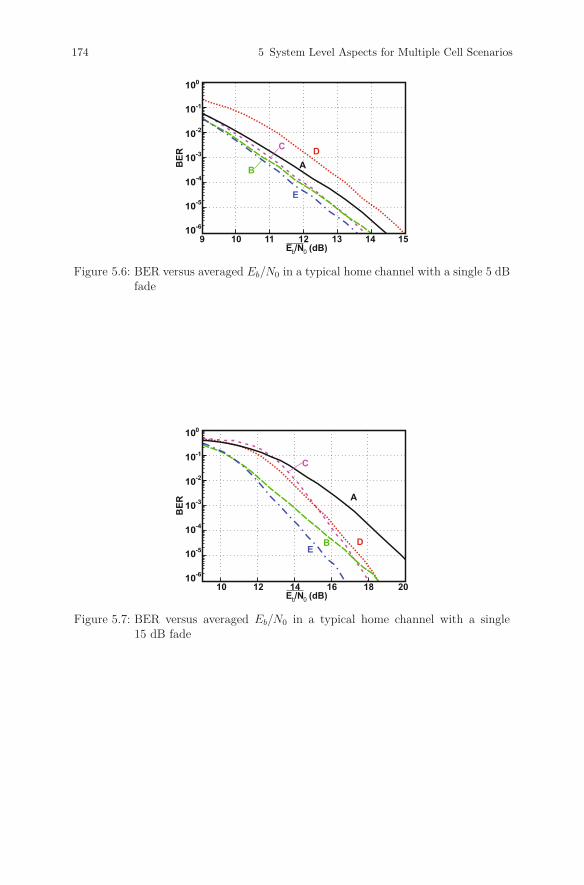
174 5 System Level Aspects for Multiple Cell Scenarios
BE
R
0bE /N (dB)
10-6
10
10-3
10-2
10-1
100
-4
AB
DC
E
10-5
9 10 11 12 13 14 15
Figure 5.6: BER versus averaged Eb/N0 in a typical home channel with a single 5 dBfade
10-6
10
10-3
10-2
10-1
100
-4
A
B D
C
E
10 12 14 16 18 20
10-5
BE
R
0bE /N (dB)
Figure 5.7: BER versus averaged Eb/N0 in a typical home channel with a single15 dB fade

5.1 Link Adaptation 175
nel selection is implemented, only channels with low fading depths will beselected in most situations. The possible improvements are thus very lim-ited. Furthermore, it should be considered that organization of adaptation ona subcarrier basis needs communication overhead for channel measurements.Another practical disadvantage is the fact that the options are not within theline of existing standards.
Link Efficiency as Optimization Criterion
Generally speaking, link efficiency of transmission systems should be optimized sothat all transmission tasks are fulfilled completely while consuming a minimum ofnetwork resources. A comparison related to Eb/N0 figures does not cover all im-portant aspects of network optimization. Therefore, an enhanced efficiency measureis needed. Discussing in terms of the ISO/OSI model, this link efficiency measureshould focus on the lower two layers. A fair comparison of different transmissionconcepts should be possible, including options of improved modulation and errorcorrection coding schemes, use of multiple antennas as well as modified MAC meth-ods. In order to derive a generic definition, we define the link efficiency by theratio between the achieved transmission performance and the consumed resources.The resources spent to achieve the transmission performance comprise the occupiedbandwidth, duration of channel occupation, and the transmit power. On this ba-sis, the efficiency of a packet transmission can be calculated as follows. The basicelement of the transmission is one symbol. However, efficiency analysis requires theinclusion of protocol overhead (of the lower two ISO/OSI layers in our case) as wellas an investigation of the trade-off between forward error correction and automaticrepeat request (ARQ) methods. Therefore, we start with the definition of the packettransmission efficiency ηP :
ηP =P L
tp · B · log2
(1 + PT ·a
(B·N0+PInt)·I) (5.1)
P L is the number of transmitted payload bits in the packet. P L equals zero, ifthe packet is not transmitted successfully (i.e., either the data packet or theacknowledgment packet associated with it is in error). Retransmissions will beconsidered when analyzing the transmission of a packet sequence.
tp is the duration of channel occupancy. It is including the transmission time ofthe data packet and the acknowledgment as well as the contention time andthe interframe spaces.
PT is the transmit power.
a is the channel attenuation factor (0 ≤ a ≤ 1) and includes free space attenua-tion and slow fading.
N0 is the spectral density of noise. As white noise is assumed, multiplication bythe bandwidth B gives the received noise power.
PInt covers interference from concurring transmissions in the same band.
176 5 System Level Aspects for Multiple Cell Scenarios
I allows introducing an implementation margin. Thus, the performance of dif-ferent implementations of network nodes can be compared. A typical value forIEEE 802.11 systems is 15 dB (10 dB noise figure plus 5 dB implementationloss).
During the transmission of each single packet, the bandwidth B, noise spectraldensity N0, implementation margin I, transmit power N0, and the interference powerPInt are assumed to be constant. During a transmission attempt there are severalphases (contention, transmission, interframe spaces), where different transmit pow-ers are used and different interference levels may occur. A temporal average of thedifferent levels seems to be inadequate when analyzing realistic network situations.For the sake of simplicity, it is proposed to assume that PT equates to the trans-mit power during the data packet transmission phase and PInt equals the maximuminterference level during this phase. The difference to the exact values will be low.Efficiency analysis should reflect the gain when the transmission conditions are im-proved, e.g., by methods to combat fast fading like diversity reception. Therefore,the severity of the hurdle of the wireless channel (as indicated by the factors a, PInt
and N0) is averaged over the duration of the link and the whole frequency band. If,for example, dynamic frequency selection is applied and a channel switch enableshigher throughput because of better transmission conditions, the effect of this linkadaptation would be directly reflected by ηP . The reason is that the ratio of P L/tp
increases, whereas a, PInt, and N0 are constant.In our analysis, the transmission of a sequence of data packets between two specific
network nodes is regarded as one link. Typically, there will be at least one source oftraffic at the transmitter side, generating packets to be sent to a receiving station.An efficiency measure on link level can be derived by using the packet transmissionefficiency as defined above and averaging over the duration of link existence. For eachtransmitted packet, the transmission efficiency ηP can be calculated. For the reasonsexplained above, only the parameters P L, tp, and PT are calculated on packet basisand therefore indexed with i. Due to packet retransmission, the number of generatedpackets NG generally will differ from the number NT of transmitted packets and thenumber of successfully decoded packets ND. To obtain the efficiency of a singlelink, ηP,i is averaged over the NT transmitted packets. This leads to the followingdefinition of link efficiency ηL:
ηL =1
NT
NT∑i=1
P Li
tp,i · B · log2
(1 +
PT,i·a(B·N0+PInt)·I
) (5.2)
The link efficiency takes into account the resources spent to achieve the perfor-mance as well as the complexity of the transmission task. It is topology independentand can be applied to different use cases. Thus, it allows a fair comparison of systemsand improvement methods.
5.1.4 Cross-Layer Adaptation
Besides the adaptation of the physical transmission parameters as discussed above,optimization also has to cover aspects of the MAC layer. Typical networks transmit

5.1 Link Adaptation 177
packets containing payload data and overhead for medium access, synchronization,and addressing. The complete bit sequence is then mapped to a number of OFDMsymbols, giving rise to another loss due to padding bits that are required to generatecomplete symbols. The size of the packet payload is crucial for achieving a highefficiency. Figure 5.8 shows the maximum throughput of one link for different grossdata rates as a function of packet size. IEEE 802.11 allows for the insertion ofa request to send / clear to send sequence to reduce the loss of capacity due tocollisions with hidden stations. Both options, with and without RTS/CTS sequence,are plotted. It is obvious that under these assumptions the maximum packet lengthyields the highest MAC throughput of 19.8 Mbit/s for the 24 Mbit/s mode withoutRTS/CTS, for example.
0 500 1000 1500 2000 25000
5
10
15
20
25
30
35
40
Packet Length (Byte)
Ne
t D
ata
Ra
te (
Mb
/s)
54o
36o
24o
54m
36m
24m
54/36/24: Gross-Data Rateo: without RTS/CTSm: with RTS/CTS
Figure 5.8: MAC throughput as a function of packet length
Up to now, the throughput has been calculated under the assumption that no col-lisions occur. A practical network comprising several transmitters will be degradeddue to collisions. The amount of collisions largely depends on the number of nodesand the kind of data traffic. If several nodes wait for a transmission opportunity,the random process decides which node will be the first to transfer. If more thanone node starts with the same backoff number a collision occurs. It turns out thatthe MAC algorithm as defined in the standard is not well suited for our scenario. Agood idea for a modified approach is to specify deterministic parameters for mediastreams which require high grades of service. Data transfers for PCs which havelow requirements with respect to delay and guaranteed data rate are assigned lowpriorities. The differentiation at the MAC layer is achieved by suitable selection ofa fixed and a variable amount of the contention window. It turns out that overallefficiency can be increased by avoiding collisions by such an approach. The achiev-able improvement depends on the scenario (number of active nodes, data rates).Simulations have shown that up to 20% increased net data rates can be achieved [9].

178 5 System Level Aspects for Multiple Cell Scenarios
5.1.5 Multiple Link Network - Overall Adaptation
Some general aspects of link adaptation have been discussed so far, focusing on thesystem scenario of media transmission in a dense environment. It turns out thatoptimization is a complex task. Many parameters, which influence each other, haveto be selected. A general link efficiency measure has been derived which allows a faircomparison of all options. Link adaptation may start on a per link basis. Even in thissimple approach, several parameters exhibit significant interdependence. Definingoptimum parameters in a complex environment is even more demanding. Further-more limitations due to standards and regulation have to be considered. Differentstrategies are possible. In the home media network described above, optimizationmay start by the selection of the best channel. In a given setup, this can be achievedby selection of the best combinations of available antenna constellation and trans-mission frequency. In the next step, the usage of this channel can be optimizedby careful selection of modulation and coding scheme. In our practical example,characterized by typical amplitude transmission functions as described above, itturns out that selecting a common scheme for all subcarriers is close to an optimumsolution. Improvements by adaptation of parameters per subcarrier would requireadditional communication overhead. A practical problem might be the fact thatsuch techniques are not allowed in existing or upcoming standards. Further roomfor significant improvements is given by selecting suitable packet sizes and MACprocedures.
Bibliography
[1] IEEE 802.11-2007, Wireless LAN Medium Access Control (MAC) and PhysicalLayer (PHY) Specifications, Jun. 2007.
[2] K. Jostschulte, R. Kays, W. Endemann, “Enhancement of Wireless LAN forMultimedia Home Networking,” IEEE Trans. on Consumer Electronics, Vol.51, No. 1, pp. 80-86, Feb. 2005.
[3] M. Lacage et al.,“IEEE 802.11 Rate Adaptation: A Practical Approach,” Proc.ACM International Conference on Modeling, Analysis and Simulation of Wire-less and Mobile Systems (MSWiM), Oct. 2004.
[4] J. Pavon et al., “Link Adaptation Strategy for IEEE 802.11 WLAN via Re-ceived Signal Strength Measurement,” Proc. IEEE International Conferenceon Communications (ICC), May 2003.
[5] I. Haratchev et al., “Automatic IEEE 802.11 Rate Control for Streaming Appli-cations,” Wireless Communications and Mobile Computing, Vol. 5, No. 4, pp.421-437, Jun. 2005.
[6] H. Koetz, R. Kays, “Efficient Dynamic Data Rate Adaptation for WirelessHome Media Networks,” Proc. International OFDM Workshop, Aug. 2008.

Bibliography 179
[7] J. Heiskala, J. Terry, OFDM Wireless LANs: A Theoretical and PracticalGuide, SAMS Publishing, Sep. 2002.
[8] K. Jostschulte, R. Kays, W. Endemann, “Optimisation of IEEE 802.11 BasedWLAN for Home Media Networks,” Proc. International OFDM Workshop,Aug./Sept. 2005.
[9] R. Kays, K. Jostschulte, W. Endemann, “Wireless Ad-Hoc Networks with HighNode Density for Home AV Transmission,” IEEE Trans. on Consumer Elec-tronics, Vol. 50, No. 2, pp. 463-471, May 2004.
180 5 System Level Aspects for Multiple Cell Scenarios
5.2 System Concept for a MIMO-OFDM-Based
Self-Organizing Data Transmission Network
C. Fellenberg, R. Grünheid, H. Rohling, Hamburg University of Technol-ogy, Germany
5.2.1 Introduction
Future wireless communication networks will provide numerous different serviceswith user-specific Quality-of-Service (QoS) demands. For this reason, flexibility aswell as adaptivity have to be considered in the system concept design, the data trans-mission technique and the medium access scheme, respectively. An efficient resourceallocation procedure in the multiple access scheme should be realized to fulfill theindividual user requirements and different data rates. The Orthogonal Frequency-Division Multiplexing (OFDM) transmission technique offers this required flexibilityand adaptivity even in multipath propagation situations and in frequency-selectiveradio channels. In the OFDM case, the total bandwidth is divided into many sub-channels which are simultaneously modulated and transmitted in a superimposedway. This allows for exploiting multi-user diversity (MUD) by the resource allocationprocedure.
Furthermore, in cellular networks, the OFDM transmission technique has theadditional advantage that all base stations and mobile terminals can be synchronizedin time and carrier frequency. In doing so, a so-called Single Frequency Network(SFN) is considered for the proposed system concept. An SFN offers high flexibilityin resource allocation as the resources can be provided to those base stations whichhave the highest traffic load. This concept is very promising, particularly for unequaluser distributions.
The OFDM transmission technique is very suitable for broadband radio channelsdue to its ability of equalization with low computation complexity. A single subcar-rier is affected by a narrowband channel and allows for multiple antenna techniques(MIMO). Therefore, in this chapter, a MIMO-OFDM based transmission techniqueis considered to achieve very high flexibility in digital transmission technique andmultiple access scheme as well as a high system performance. Especially, beamform-ing techniques are treated, allowing for multiple users to be served on the same timefrequency resource. Thus, the resources to be allocated are separated in space, time,and frequency. Moreover, depending on the channel knowledge at the transmitter,different antenna diagrams and beam patterns are applicable.
The resource allocation scheme is integrated into the scheduler. Based on the op-timization objectives (fairness, capacity, ...), the scheduling procedure is organizedin a cross-layer approach by taking the QoS parameters of the data link control(DLC) layer as well as the radio channel knowledge of the physical layer into ac-count. The goal of this chapter is to design and develop a system concept for futurewireless cellular communication networks, based on the MIMO-OFDM transmissiontechnique and related multiple access schemes. The resource allocation is performedin a self-organized procedure.
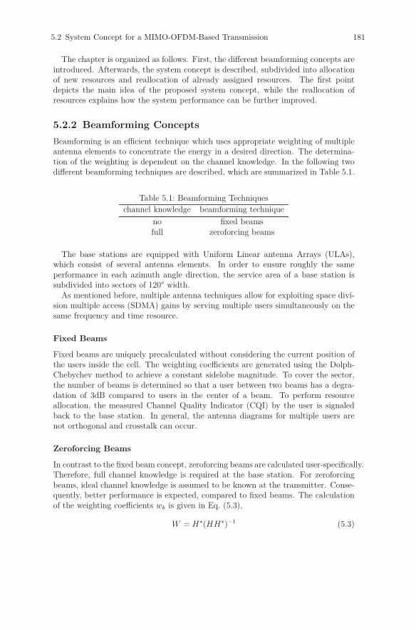
5.2 System Concept for a MIMO-OFDM-Based Transmission 181
The chapter is organized as follows. First, the different beamforming concepts areintroduced. Afterwards, the system concept is described, subdivided into allocationof new resources and reallocation of already assigned resources. The first pointdepicts the main idea of the proposed system concept, while the reallocation ofresources explains how the system performance can be further improved.
5.2.2 Beamforming Concepts
Beamforming is an efficient technique which uses appropriate weighting of multipleantenna elements to concentrate the energy in a desired direction. The determina-tion of the weighting is dependent on the channel knowledge. In the following twodifferent beamforming techniques are described, which are summarized in Table 5.1.
Table 5.1: Beamforming Techniqueschannel knowledge beamforming technique
no fixed beamsfull zeroforcing beams
The base stations are equipped with Uniform Linear antenna Arrays (ULAs),which consist of several antenna elements. In order to ensure roughly the sameperformance in each azimuth angle direction, the service area of a base station issubdivided into sectors of 120° width.
As mentioned before, multiple antenna techniques allow for exploiting space divi-sion multiple access (SDMA) gains by serving multiple users simultaneously on thesame frequency and time resource.
Fixed Beams
Fixed beams are uniquely precalculated without considering the current position ofthe users inside the cell. The weighting coefficients are generated using the Dolph-Chebychev method to achieve a constant sidelobe magnitude. To cover the sector,the number of beams is determined so that a user between two beams has a degra-dation of 3dB compared to users in the center of a beam. To perform resourceallocation, the measured Channel Quality Indicator (CQI) by the user is signaledback to the base station. In general, the antenna diagrams for multiple users arenot orthogonal and crosstalk can occur.
Zeroforcing Beams
In contrast to the fixed beam concept, zeroforcing beams are calculated user-specifically.Therefore, full channel knowledge is required at the base station. For zeroforcingbeams, ideal channel knowledge is assumed to be known at the transmitter. Conse-quently, better performance is expected, compared to fixed beams. The calculationof the weighting coefficients wk is given in Eq. (5.3),
W = H∗(HH∗)−1 (5.3)

182 5 System Level Aspects for Multiple Cell Scenarios
where the matrix H comprises the channel vectors hk of the considered usersand matrix W consists of the corresponding weighting vectors wk. By means ofzeroforcing beams, intra-sector interference is completely avoided for the consideredusers.
For zeroforcing beams the question arises which users should be served simultane-ously on the same frequency resource. Here, heuristic grouping approaches are used,exploiting, e.g., the orthogonality of the channel vectors [4]. In [5] new algorithmswere proposed to exploit SDMA as well as MUD gains.
5.2.3 System Concept
MT 1
MT 5
MT 2
MT 4
MT 3
BS
BS
BSBS
BS
BS 2
BS 1
Resource
RX
Pow
er MT1MT2
BS 1
Resource
RX
Pow
er MT1MT2
BS 1
RX
Pow
er
MT3
MT4MT5
BS 2
Resource
Figure 5.9: Cellular Network
This section covers the design of the proposed system concept for a MIMO-OFDMtransmission system in the described context. The scheduling of resources is basedon the CQI and the QoS parameters of the users. In addition, the cellular network isassumed to be totally synchronized in time and frequency to fulfill the requirement ofsingle frequency networks supporting point-to-point connections (Fig. 5.9). In [3] it isshown that the synchronization in an OFDM based cellular network is feasible. Dueto the carrier synchronization, the interference of neighboring cells is only observedas co-channel interference. The base stations are equipped with multiple antennas,while the mobile terminals make use of a single antenna. A time division duplex(TDD) scheme is applied to separate the down- and uplink for data transmission.
The philosophy of the system concept is to incorporate high flexibility into thesystem while keeping the interference on a low level. The self-organizing approachis based on measurable and predictable interference situations in the network. Inthis way, the mobile terminals as well as the base stations are able to measure theinterference situation and allocate appropriate resources. While the interferenceis different for the base station and the mobile terminal, the useful power is the
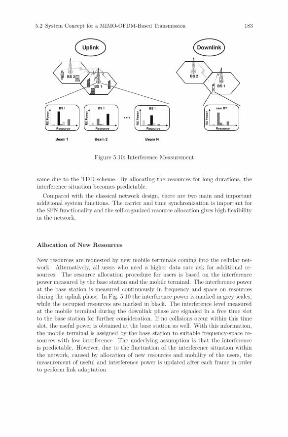
5.2 System Concept for a MIMO-OFDM-Based Transmission 183
BS 1
BS 2
Beam 1 Beam 2 Beam N
…
BS 1
Resource
RX
Po
wer
BS 1
Resource
RX
Po
wer
BS 1
Resource
RX
Po
wer
new MT
Resource
RX
Po
wer
BS 1
BS 2
Uplink Downlink
Figure 5.10: Interference Measurement
same due to the TDD scheme. By allocating the resources for long durations, theinterference situation becomes predictable.
Compared with the classical network design, there are two main and importantadditional system functions. The carrier and time synchronization is important forthe SFN functionality and the self-organized resource allocation gives high flexibilityin the network.
Allocation of New Resources
New resources are requested by new mobile terminals coming into the cellular net-work. Alternatively, all users who need a higher data rate ask for additional re-sources. The resource allocation procedure for users is based on the interferencepower measured by the base station and the mobile terminal. The interference powerat the base station is measured continuously in frequency and space on resourcesduring the uplink phase. In Fig. 5.10 the interference power is marked in grey scales,while the occupied resources are marked in black. The interference level measuredat the mobile terminal during the downlink phase are signaled in a free time slotto the base station for further consideration. If no collisions occur within this timeslot, the useful power is obtained at the base station as well. With this information,the mobile terminal is assigned by the base station to suitable frequency-space re-sources with low interference. The underlying assumption is that the interferenceis predictable. However, due to the fluctuation of the interference situation withinthe network, caused by allocation of new resources and mobility of the users, themeasurement of useful and interference power is updated after each frame in orderto perform link adaptation.
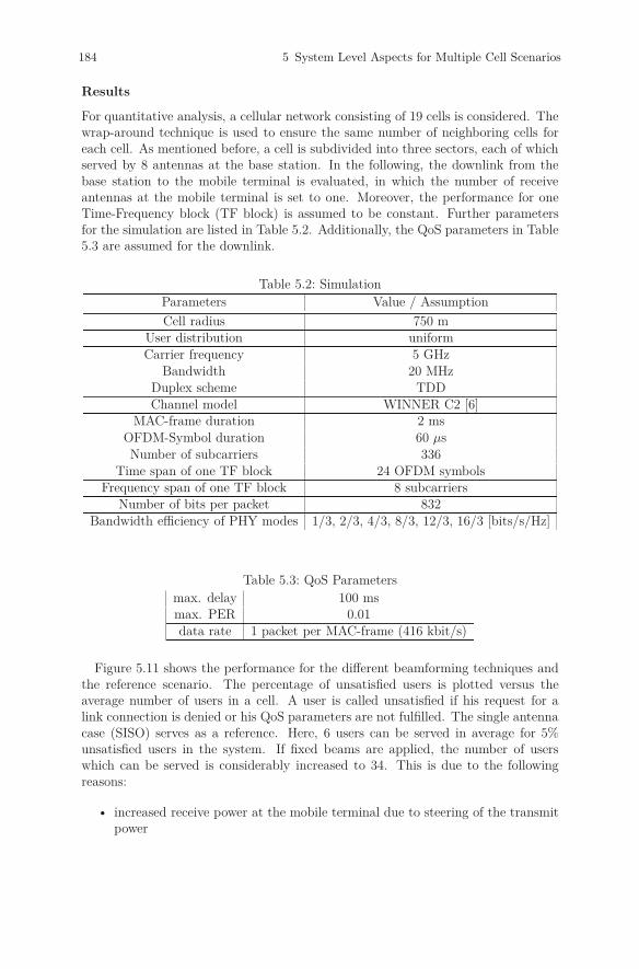
184 5 System Level Aspects for Multiple Cell Scenarios
Results
For quantitative analysis, a cellular network consisting of 19 cells is considered. Thewrap-around technique is used to ensure the same number of neighboring cells foreach cell. As mentioned before, a cell is subdivided into three sectors, each of whichserved by 8 antennas at the base station. In the following, the downlink from thebase station to the mobile terminal is evaluated, in which the number of receiveantennas at the mobile terminal is set to one. Moreover, the performance for oneTime-Frequency block (TF block) is assumed to be constant. Further parametersfor the simulation are listed in Table 5.2. Additionally, the QoS parameters in Table5.3 are assumed for the downlink.
Table 5.2: SimulationParameters Value / Assumption
Cell radius 750 mUser distribution uniformCarrier frequency 5 GHz
Bandwidth 20 MHzDuplex scheme TDDChannel model WINNER C2 [6]
MAC-frame duration 2 msOFDM-Symbol duration 60 μsNumber of subcarriers 336
Time span of one TF block 24 OFDM symbolsFrequency span of one TF block 8 subcarriers
Number of bits per packet 832Bandwidth efficiency of PHY modes 1/3, 2/3, 4/3, 8/3, 12/3, 16/3 [bits/s/Hz]
Table 5.3: QoS Parametersmax. delay 100 msmax. PER 0.01data rate 1 packet per MAC-frame (416 kbit/s)
Figure 5.11 shows the performance for the different beamforming techniques andthe reference scenario. The percentage of unsatisfied users is plotted versus theaverage number of users in a cell. A user is called unsatisfied if his request for alink connection is denied or his QoS parameters are not fulfilled. The single antennacase (SISO) serves as a reference. Here, 6 users can be served in average for 5%unsatisfied users in the system. If fixed beams are applied, the number of userswhich can be served is considerably increased to 34. This is due to the followingreasons:
• increased receive power at the mobile terminal due to steering of the transmitpower

5.2 System Concept for a MIMO-OFDM-Based Transmission 185
• SDMA gains
• better interference situation within the system
0 5 10 15 20 25 30 35 40 45 50 550
1
2
3
4
5
6
7
8
9
10
average number of users per cell
unsa
tisfie
d us
ers
[%]
SISOMISO, Fixed BeamsMISO, ZF Beams
28 10
Figure 5.11: Allocation of New Resources
The last point is visualized in Fig. 5.12, where a cellular system and a single subcar-rier are considered. The receive power is plotted for all base stations from one mobileterminal localized at the green cross. The dark blue color represents the noise powerwhile the dark red color represents high signal power. Obviously, for the MISOsystem lots of more resources are still usable for every base station compared to theSISO system.
SISO
MISO
Figure 5.12: Interference at BS
Expectedly, the zeroforcing beams achieve the highest performance, yielding anincrease of 10 users compared to fixed beams. Beside the advantages of the MISOsystem pointed out before, the ideal channel knowledge is exploited so that intra-sector interference is fully avoided. Additionally, the steering of transmit powertowards the users is enhanced.
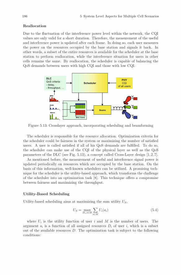
186 5 System Level Aspects for Multiple Cell Scenarios
Reallocation
Due to the fluctuation of the interference power level within the network, the CQIvalues are only valid for a short duration. Therefore, the measurement of the usefuland interference power is updated after each frame. In doing so, each user measuresthe power on the resources occupied by the base station and signals it back. Inother words, a subset of the entire resources is available for the scheduler at the basestation to perform reallocation, while the interference situation for users in othercells remains the same. By reallocation, the scheduler is capable of balancing theQoS demands between users with high CQI and those with low CQI.
Scheduler
PHY
CQI
of all users
DLC
QoS criteria:
- delay,
- throughput, …
MPEG
Audio
Ethernet
t
t
t
MPEG
Audio
Ethernet
t
t
t
MAC frame
MT 1
MT 2
MT 3
Beams
Figure 5.13: Crosslayer approach, incorporating scheduling and beamforming
The scheduler is responsible for the resource allocation. Optimization criteria forthe scheduler could be fairness in the system or maximizing the number of satisfiedusers. A user is called satisfied if all of his QoS demands are fulfilled. To do so,the scheduler can make use of the CQI of the physical layer as well as the QoSparameters of the DLC (see Fig. 5.13), a concept called Cross-Layer design [1, 2, 7].
As mentioned before, the measurement of useful and interference signal power isupdated periodically on resources which are occupied by the base station. On thebasis of this information, well-known schedulers can be utilized. A promising tech-nique for the scheduler is the utility-based approach, which transforms the challengeof the scheduler into an optimization task [8]. This technique offers a compromisebetween fairness and maximizing the throughput.
Utility-Based Scheduling
Utility-based scheduling aims at maximizing the sum utility US,
US = maxDi,i∈M
∑i∈M
Ui(ai) (5.4)
where Ui is the utility function of user i and M is the number of users. Theargument ai is a function of all assigned resources Di of user i, which is a subsetout of the available resources D. The optimization task is subject to the followingconditions:

5.2 System Concept for a MIMO-OFDM-Based Transmission 187
M⋃i=1
Di ⊆ D
Di
⋂Dj = ∅, i �= j
An appropriate choice of the utility function for each user is dependent on theoptimization task (e.g., capacity, fairness, QoS demands of the users). In the scopeof this project, different utility functions have been considered.
Data Rate-Based Utility Function
For the data rate based utility function, the argument ai in Eq. (5.4) represents theoverall data rate ri for one MAC-frame, assigned to user i. The overall data rate isgiven by the sum of data rates ci,d on single resources d.
ai = ri =∑
d∈Di
ci,d
So far, solving the optimization task yields the resource allocation for one MAC-frame. However, fairness and QoS demands are related to time. Therefore, a low-pass filter is used for the sum of data rates in order to exploit the time dimension.
ri(n) = αri(n − 1) + (1 − α)ri(n)
As a matter of fact, the argument ai in Eq. 5.4 is replaced by ri(n). Fairnessamong the users is achieved by a logarithmic slope of the utility function. In thisway, users with a relatively low data rate are preferred for the resource allocation.In literature this kind of scheduling is well-known as proportional fair scheduling(PFS) [9]. Certainly, PFS evaluates pure channel state information. In order tomaximize the number of satisfied users, it is self-evident that information from theDLC has to be incorporated into the progression of the utility function. This is,e.g., achieved with modified largest weighted delay first (M-LWDF) scheduling [10]by weighting the logarithmic slope of the utility function with the waiting time ofthe first packet in the queue Ti. Thus, also users with a large waiting time of thefirst packet in the queue are preferred for resource allocation. The resulting utilityfunction is given in Eq. (5.5).
Ui(ri(n)) =
⎧⎨⎩Tilog(ri(n)) , ri(n) ≤ rmax,i(n)
Tilog(rmax,i(n)) , ri(n) > rmax,i(n)(5.5)
The parameter rmax,i(n) ensures that the assigned data rate for user i is notfurther increased if there are no more packets in his queue. Fig. 5.14 shows thecharacteristics of the utility function for different users and waiting times of the firstpackets. The optimization task is expressed as follows:
US = maxDi,i∈M
∑i∈M
Ui(ri(n))
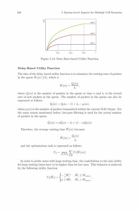
188 5 System Level Aspects for Multiple Cell Scenarios
ri
Ui(r
i)
rmax,1 rmax,2rmax,3
user 1
user 3
user 2
Figure 5.14: Data Rate-based Utility Function
Delay-Based Utility Function
The idea of the delay based utility function is to minimize the waiting time of packetsin the queue Wi(n) [11], which is
Wi(n) =Qi(n)
λi
,
where Qi(n) is the number of packets in the queue at time n and λi is the arrivalrate of new packets in the queue. The number of packets in the queue can also beexpressed as follows
Qi(n) = Qi(n − 1) + λi − pi(n),
where pi(n) is the number of packets transmitted within the current MAC-frame. Forthe same reason mentioned before, low-pass filtering is used for the actual numberof packets in the queue.
Qi(n) = αQi(n − 1) + (1 − α)Qi(n)
Therefore, the average waiting time Wi(n) becomes
Wi(n) =Qi(n)
λi
and the optimization task is expressed as follows.
US = maxDi,i∈M
∑i∈M
Ui(Wi(n))
In order to prefer users with large waiting time, the contribution to the sum utilityfor large waiting times have to be higher than for low ones. This behavior is achievedby the following utility function
Ui(Wi) =
⎧⎨⎩− 1
γiW γi
i , Wi ≤ Wmax,i
a + bWi , Wi > Wmax,i
,
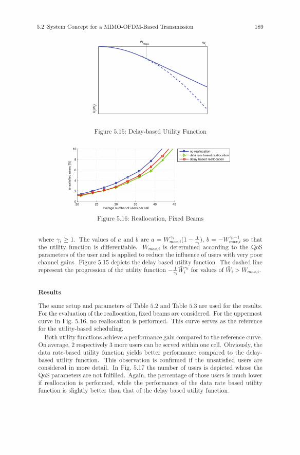
5.2 System Concept for a MIMO-OFDM-Based Transmission 189
Wi
Ui(W
i)
Wmax,i
Figure 5.15: Delay-based Utility Function
20 25 30 35 40 450
2
4
6
8
10
average number of users per cell
unsa
tisfie
d us
ers
[%]
no reallocationdata rate based reallocationdelay based reallocation
Figure 5.16: Reallocation, Fixed Beams
where γi ≥ 1. The values of a and b are a = W γimax,i(1 − 1
γi), b = −W γi−1
max,i so thatthe utility function is differentiable. Wmax,i is determined according to the QoSparameters of the user and is applied to reduce the influence of users with very poorchannel gains. Figure 5.15 depicts the delay based utility function. The dashed linerepresent the progression of the utility function − 1
γiW γi
i for values of Wi > Wmax,i.
Results
The same setup and parameters of Table 5.2 and Table 5.3 are used for the results.For the evaluation of the reallocation, fixed beams are considered. For the uppermostcurve in Fig. 5.16, no reallocation is performed. This curve serves as the referencefor the utility-based scheduling.
Both utility functions achieve a performance gain compared to the reference curve.On average, 2 respectively 3 more users can be served within one cell. Obviously, thedata rate-based utility function yields better performance compared to the delay-based utility function. This observation is confirmed if the unsatisfied users areconsidered in more detail. In Fig. 5.17 the number of users is depicted whose theQoS parameters are not fulfilled. Again, the percentage of those users is much lowerif reallocation is performed, while the performance of the data rate based utilityfunction is slightly better than that of the delay based utility function.
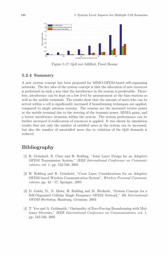
190 5 System Level Aspects for Multiple Cell Scenarios
20 25 30 35 400
0.2
0.4
0.6
0.8
1
1.2
1.4
1.6
average number of users per cell
QoS
not
fulfi
lled
[%]
no reallocationdata rate based reallocationdelay based reallocation
Figure 5.17: QoS not fulfilled, Fixed Beams
5.2.4 Summary
A new system concept has been proposed for MIMO-OFDM-based self-organizingnetworks. The key idea of the system concept is that the allocation of new resourcesis performed in such a way that the interference in the system is predictable. There-fore, interference can be kept on a low level by measurement at the base stations aswell as the mobile terminals. The results show that the amount of users who can beserved within a cell is significantly increased if beamforming techniques are applied,compared to single antenna systems. The reasons are the increased receive powerat the mobile terminal due to the steering of the transmit power, SDMA gains, anda better interference situation within the system. The system performance can befurther increased if reallocation of resources is applied. It was shown by simulationresults that not only the number of satisfied users in the system can be increased,but also the number of unsatisfied users due to violation of the QoS demands isreduced.
Bibliography
[1] R. Grünheid, B. Chen and H. Rohling, “Joint Layer Design for an AdaptiveOFDM Transmission System,” IEEE International Conference on Communi-cations, vol. 1, pp. 542-546, 2005
[2] H. Rohling and R. Grünheid, “Cross Layer Considerations for an AdaptiveOFDM-based Wireless Communication System”, Wireless Personal Communi-cations, pp. 43 - 57, Springer, 2005
[3] D. Galda, D., N. Meier, H. Rohling and M. Weckerle, “System Concept for aSelf-Organized Cellular Single Frequency OFDM Network,” 8th InternationalOFDM-Workshop, Hamburg, Germany, 2003
[4] T. Yoo and A. Goldsmith, “Optimality of Zero-Forcing Beamforming with Mul-tiuser Diversity,” IEEE International Conference on Communications, vol. 1,pp. 542-546, 2005
Bibliography 191
[5] C. Fellenberg, A. Tassoudji, R. Grünheid and H. Rohling, “QoS aware Schedul-ing in Combination with Zero-Forcing Beamforming Techniques in MIMO-OFDM based Transmission Systems,” 14th International OFDM-Workshop,Hamburg, Germany, 2009
[6] WINNER “System Concept Descritpion”, Deliverable D7.6, IST-2003-507581WINNER, 2005
[7] R. Grünheid, B. Chen and H. Rohling, “Joint Layer Design for an AdaptiveOFDM Transmission System,” IEEE International Conference on Communi-cations, vol. 1, pp. 542-546, 2005
[8] G. Song and Y. Li, “Utility-Based Resource Allocation and Scheduling inOFDM-Based Wireless Broadband Networks,” IEEE Communications Maga-zine, vol. 43, no. 12, pp. 127-134, 2005
[9] H. Kim and Y. Han, “A Proportional Fair Scheduling for Multicarrier Trans-mission Systems,” IEEE Communications Letters, vol. 9, no. 3, 2005
[10] M. Andrews, K. Kumaran, K. Ramanan, A. Stolyar, P. Whiting and R. Vi-jayakumar, “Providing Quality of Service over a Shared Wireless Link,” IEEECommunications Magazine, pp. 150-154, 2001
[11] G. Song, Y. Li, L. J. Cimini, Jr., H. Zheng,“Joint Channel-Aware and Queue-Aware Data Scheduling in Multiple Shared Wireless Channels,” IEEE WirelessCommunications and Networking Conference, vol. 3, pp. 1939-1944, 2004
192 5 System Level Aspects for Multiple Cell Scenarios
5.3 Pricing Algorithms for Power Control,
Beamformer Design, and Interference
Alignment in Interference Limited Networks
D. Schmidt, W. Utschick, Technische Universität München, Germany
5.3.1 Introduction
In this chapter, we examine the problem of finding good resource allocations innetworks of many interfering transmitter-receiver pairs, where the receivers are notable to decode the signals from any but the desired transmitter and thus must treatinterference as noise. While one approach in such systems is to allocate resourcesorthogonally (e. g., by assigning separate time slots or frequency bands to the trans-mitters), it will often be advantageous to allow users to share the resources to someextent. The transmit strategies must then, however, be optimized in order to reducethe negative effects of interference as much as possible.
The resulting optimization problems turn out to have undesirable properties: mul-tiple (locally optimal) solutions to the necessary optimality conditions may exist, andthese solutions in general cannot be explicitly computed. Therefore, it is necessaryto rely on iterative algorithms to determine the transmit strategies. Also, due tothe decentralized nature of the underlying system model, special attention must bepayed to the distributed implementability of the algorithms.
Multiple antennas at the transmitters or receivers allow for spatial interferenceavoidance, where, e. g., a transmitter can focus its beam in the direction of itsintended receiver and away from the unintended receivers. In MIMO systems, fur-thermore, the issue of interference alignment arises, leading to a whole new class ofhigh-SNR optimal strategies.
5.3.2 System Model
We examine a system with K transmitter-receiver pairs (synonymously called users),where each receiver is only interested in the signal from its associated transmitterand all interference is treated as additional noise. Each receiver (transmitter) hasM (N) antennas, respectively. The received signal vector of user k is
yk = Hkkxk︸ ︷︷ ︸desired signal
+∑j �=k
Hkjxj
︸ ︷︷ ︸interference
+ nk︸︷︷︸noise
, (5.6)
where Hkj ∈ CM×N is the matrix of channel coefficients between transmitter j andreceiver k, xj ∈ CN is the vector of symbols transmitted by transmitter j, andnk ∈ CM is the noise experienced at the M antennas of receiver k.
We assume the noise vector nk to be uncorrelated with variance σ2
E[nkn
H
k
]= σ2I, (5.7)
5.3 Pricing Algorithms 193
and impose a unit power constraint on the transmit vector at each transmitter:
E[‖xk‖2
2
]≤ 1. (5.8)
The receive and transmit processing of user k is performed by the filter vectorsgk ∈ CM and vk ∈ CN , respectively. Note that for the sake of notational simplicitywe limit ourselves to one data stream per user. The transmit vector xk is obtainedby multiplying the data symbol sk with the beamformer vk:
xk = vksk. (5.9)
For unit variance data symbols, this implies that the transmit power constraint (5.8)can be written as
‖vk‖22 ≤ 1. (5.10)
After processing the received signal yk with the receive filter vector gk, the estimatesk of the data symbol sk is
sk = gH
k yk = gH
k Hkkvksk︸ ︷︷ ︸desired signal
+∑j �=k
gH
k Hkjvjsj
︸ ︷︷ ︸interference
+ gH
k nk︸ ︷︷ ︸noise
. (5.11)
The favorability of a certain situation to user k can be measured by its signal tointerference-plus-noise ratio (SINR)
γk =|gH
k Hkkvk|2∑j �=k|gH
k Hkjvj|2 + σ2‖gk‖22
=Sk
Ik + Nk, (5.12)
where Sk, Ik, and Nk are the desired signal power, interference power, and noisepower after the receive filter, respectively. The goal is to maximize the system-widesum utility, where each user’s utility uk(γk) is an increasing function of its SINR:
maxv1,...,vKg1,...,gK
K∑k=1
uk(γk) s. t.: ‖vk‖22 ≤ 1 ∀k ∈ {1, . . . , K}. (5.13)
For many relevant utility functions (such as the ‘rate’ utility uk(γk) = log(1 + γk),which is of special relevance since it can be interpreted as the achievable rate withGaussian signaling), this problem is non-convex and requires a global optimizationalgorithm.
While suitable global optimization techniques exist (cf. [8]), they quickly becomeprohibitively complex with increasing system dimensions. In this work, we insteadfocus on finding good local optima by means of iterative algorithms.
5.3.3 Distributed Interference Pricing
Power Control in SISO Systems
We first examine the single-input single-output (SISO) case, where each transmittingor receiving terminal has a single antenna, i. e., N = M = 1. In this case, transmit

194 5 System Level Aspects for Multiple Cell Scenarios
filters, channel coefficients, and receivers are all scalars, and we write them as gk,hkj, and vk, respectively. Since it is clear from (5.12) that the value of gk is irrelevantfor the SINR, we assume gk = 1 ∀k, w. l. o. g. Likewise, the SINR only depends onthe squared magnitude of vk, so we use the abbreviation pk = |vk|2.
We define the interference price πk of user k as the marginal decrease of the utilityuk(γk) with the increase in received interference power Ik, evaluated at the currentoperating point:
πk = −∂uk(γk)
∂Ik
=∂uk(γk)
∂γk
· Sk
(Ik + Nk)2. (5.14)
In our iterative algorithm, each transmitter updates its transmit power pk takinginto account the interference prices of all other users:
pnewk = argmax
pk
uk(γk) − ∑j �=k
πj|hjk|2pk s. t.: 0 ≤ pk ≤ 1. (5.15)
The rationale behind this update rule is that instead of selfishly maximizing itsown utility uk(γk), which would lead to every user always transmitting with fullpower pk = 1, the user should maximize the own utility minus the ‘cost’ of causinginterference to others. We can also interpret (5.15) as maximizing an approximatedsum utility (cf. (5.13)), where all utility terms of the other users are linearized aroundthe current operating point:
uj(γj) ≈ ∂uj(γj)
∂Ij
· ∂Ij
∂pk
∣∣∣∣∣Op. Point
· pk + c = −πj|hjk|2pk + c. (5.16)
The constant c does not depend on pk and is therefore irrelevant to the optimizationproblem (5.15).
The distributed interference pricing algorithm works as follows:
1. All transmit powers pk are initialized (e. g., with unit power).
2. Each user k computes the interference price πk according to (5.14) and an-nounces it to all other users.
3. The users update their transmit strategies (powers, in the SISO case) accordingto (5.15).
4. Repeat from 2. until convergence.
It can be easily shown that, once this algorithm has converged, the Karush-Kuhn-Tucker (KKT) conditions of the original sum utility problem (5.13) are fulfilled,i. e., a local optimum has been found. Further convergence properties depend on theutility functions; for a detailed analysis, cf. [3].
Beamformer Design in MISO Systems
Next, we examine the multiple-input single-output (MISO) scenario, where all trans-mitters have N > 1 antennas while the receivers have M = 1 antennas each. The
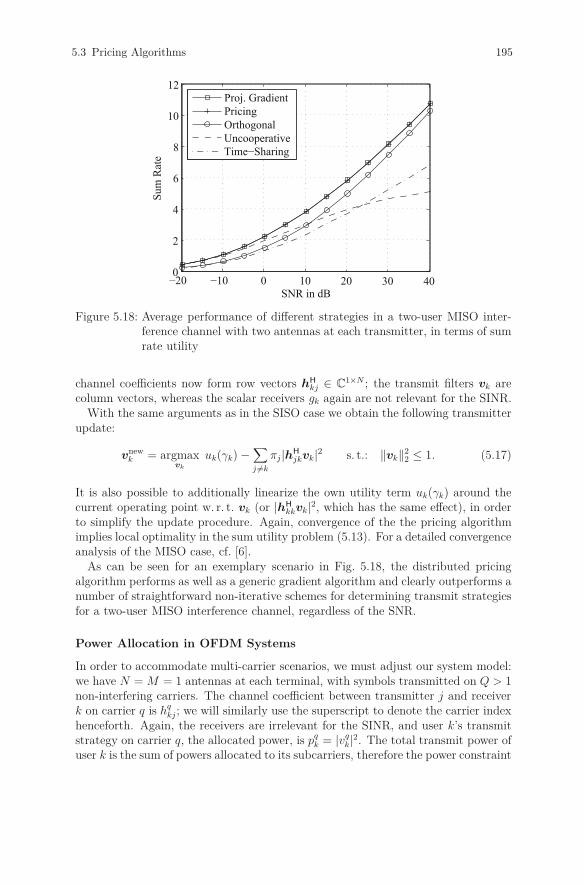
5.3 Pricing Algorithms 195
−20 −10 0 10 20 30 400
2
4
6
8
10
12
SNR in dB
Sum
Rat
e
Proj. GradientPricingOrthogonalUncooperativeTime−Sharing
Figure 5.18: Average performance of different strategies in a two-user MISO inter-ference channel with two antennas at each transmitter, in terms of sumrate utility
channel coefficients now form row vectors hH
kj ∈ C1×N ; the transmit filters vk arecolumn vectors, whereas the scalar receivers gk again are not relevant for the SINR.
With the same arguments as in the SISO case we obtain the following transmitterupdate:
vnewk = argmax
vk
uk(γk) − ∑j �=k
πj|hH
jkvk|2 s. t.: ‖vk‖22 ≤ 1. (5.17)
It is also possible to additionally linearize the own utility term uk(γk) around thecurrent operating point w. r. t. vk (or |hH
kkvk|2, which has the same effect), in orderto simplify the update procedure. Again, convergence of the the pricing algorithmimplies local optimality in the sum utility problem (5.13). For a detailed convergenceanalysis of the MISO case, cf. [6].
As can be seen for an exemplary scenario in Fig. 5.18, the distributed pricingalgorithm performs as well as a generic gradient algorithm and clearly outperforms anumber of straightforward non-iterative schemes for determining transmit strategiesfor a two-user MISO interference channel, regardless of the SNR.
Power Allocation in OFDM Systems
In order to accommodate multi-carrier scenarios, we must adjust our system model:we have N = M = 1 antennas at each terminal, with symbols transmitted on Q > 1non-interfering carriers. The channel coefficient between transmitter j and receiverk on carrier q is hq
kj ; we will similarly use the superscript to denote the carrier indexhenceforth. Again, the receivers are irrelevant for the SINR, and user k’s transmitstrategy on carrier q, the allocated power, is pq
k = |vqk|2. The total transmit power of
user k is the sum of powers allocated to its subcarriers, therefore the power constraint

196 5 System Level Aspects for Multiple Cell Scenarios
isQ∑
q=1
pqk ≤ 1 ∀k. (5.18)
With similarly defined SINR γqk, utility uq
k(γqk), and interference price πq
k for carrierq of user k, the update rule for user k in a multi-carrier system is:
{p1,newk , . . . , pQ,new
k } = argmax{p1
k,...,pQk }
Q∑q=1
uqk(γq
k) − ∑j �=k
Q∑q=1
πqj |hq
jk|2pqk
s. t.:Q∑
q=1
pqk ≤ 1 and pq
k ≥ 0 ∀q.
(5.19)
The algorithm is proposed and analyzed in detail in [3].
5.3.4 MIMO Interference Networks and InterferenceAlignment
The distributed pricing algorithm can also be extended to multiple-input multiple-output (MIMO) scenarios, where both N > 1 and M > 1. In contrast to allpreviously discussed scenarios, the receive filters gk are now relevant for the SINR.They must be continually updated in order to maximize the received SINR andmust also be communicated to the other users alongside the interference prices. Fora more detailed description of the algorithm, cf. [7].
In some cases, however, the full potential of the system is not achieved withthe pricing algorithm. Let us consider, for example, a scenario with N = M = 2antennas at all terminals, K = 3 users, and high SNR, where the goal is to maximizethe sum rate utility
∑k log(1+γk). The pricing algorithm in general will converge to
a solution in which two users are active and the interference power after their receivefilters gk is close to zero. It is, however, possible to transmit three interference-freestreams (one for each user) in this setting by ensuring that at each receiver theinterference from both undesired transmitters is collinear and thus separable fromthe desired signal, i. e., by fulfilling the three conditions
H12v2 ‖ H13v3, H21v1 ‖ H23v3, and H31v1 ‖ H32v2, (5.20)
while using all available power at each transmitter, i. e., ‖vk‖22 = 1 ∀k. Note that
for these conditions the number of equations equals the number of variables and itcan be shown that they are always feasible. Clearly, for sufficiently high SNR, threeseparate data streams will lead to a higher sum rate utility than two.
These high-SNR optimal solutions are called interference aligned [1]. Due to theproperties of the sum rate utility, interference aligned solutions are not easy to findby performing gradient based algorithms on the utility function. Two distributedalgorithms specifically aimed at finding aligned solutions have been proposed in [2]:the ‘min leakage’ and ‘max SINR’ algorithms, both based on a heuristic of repeatedlyexchanging the roles of transmitters and receivers. The former, while its convergenceis guaranteed, is clearly suboptimal for moderate and lower SNR, as it attempts to
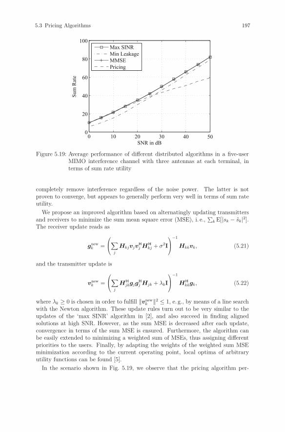
5.3 Pricing Algorithms 197
0 10 20 30 40 500
20
40
60
80
100
SNR in dB
Sum
Rat
e
Max SINRMin LeakageMMSEPricing
Figure 5.19: Average performance of different distributed algorithms in a five-userMIMO interference channel with three antennas at each terminal, interms of sum rate utility
completely remove interference regardless of the noise power. The latter is notproven to converge, but appears to generally perform very well in terms of sum rateutility.
We propose an improved algorithm based on alternatingly updating transmittersand receivers to minimize the sum mean square error (MSE), i. e.,
∑k E[|sk − sk|2].
The receiver update reads as
gnewk =
⎛⎝∑
j
HkjvjvH
j HH
kj + σ2I
⎞⎠−1
Hkkvk, (5.21)
and the transmitter update is
vnewk =
⎛⎝∑
j
HH
jkgjgH
j Hjk + λkI
⎞⎠−1
HH
kkgk, (5.22)
where λk ≥ 0 is chosen in order to fulfill ‖vnewk ‖2 ≤ 1, e. g., by means of a line search
with the Newton algorithm. These update rules turn out to be very similar to theupdates of the ‘max SINR’ algorithm in [2], and also succeed in finding alignedsolutions at high SNR. However, as the sum MSE is decreased after each update,convergence in terms of the sum MSE is ensured. Furthermore, the algorithm canbe easily extended to minimizing a weighted sum of MSEs, thus assigning differentpriorities to the users. Finally, by adapting the weights of the weighted sum MSEminimization according to the current operating point, local optima of arbitraryutility functions can be found [5].
In the scenario shown in Fig. 5.19, we observe that the pricing algorithm per-
198 5 System Level Aspects for Multiple Cell Scenarios
forms well for moderate and low SNR, but does not achieve the full high-SNR slope(i. e., number of interference-free data streams). The ‘min leakage’ algorithm [2]does achieve the maximum slope, but is clearly suboptimal to the ‘max SINR’ al-gorithm [2] as well as the MMSE approach discussed above, which both achieve asimilar sum utility in this case.
5.3.5 Summary
We have presented distributed algorithms for different types of interference networks,in which determining the globally optimal transmit strategy is not feasible. Whilefor SISO, MISO, and OFDM systems the distributed interference pricing algorithmfinds good locally optimal configurations, MIMO systems that allow for interferencealignment require a different class of algorithm in order to achieve full system poten-tial at high SNR. Here, minimizing the weighted sum MSE is a promising approachin addition to the algorithms in [2].
A comprehensive overview of pricing algorithms for interference networks can befound in [4].
Bibliography
[1] V. R. Cadambe and S. A. Jafar, “Interference alignment and degrees of freedomof the K-user interference channel,” 54(8):3425–3441, August 2008.
[2] K. Gomadam, V. R. Cadambe, and S. A. Jafar, “Approaching the capacity ofwireless networks through distributed interference alignment,” in Proc. IEEEGlobal Commun. Conf. (GLOBECOM), New Orleans, LA, November 2008.
[3] J. Huang, R. A. Berry, and M. L. Honig, “Distributed interference compensationfor wireless networks,” 24(5):1074–1084, May 2006.
[4] D. A. Schmidt, C. Shi, R. A. Berry, M. L. Honig, and W. Utschick, “Distributedresource allocation schemes,” 26(5):53–63, September 2009.
[5] D. A. Schmidt, C. Shi, R. A. Berry, M. L. Honig, and W. Utschick, “Mini-mum mean squared error interference alignment,” in Proc. 43rd Asilomar Conf.Signals, Syst., Comput., Pacific Grove, CA, November 2009.
[6] C. Shi, R. A. Berry, and M. L. Honig, “Distributed interference pricing withMISO channels,” in Proc. 46th Annu. Allerton Conf. Commun., Control, Com-puting, Monticello, IL, September 2008.
[7] C. Shi, D. A. Schmidt, R. A. Berry, M. L. Honig, and W. Utschick, “Distributedinterference pricing for the MIMO interference channel,” in Proc. IEEE Int.Conf. Commun., Dresden, Germany, June 2009.
[8] H. Tuy, “Monotonic optimization: Problems and solution approaches,” SIAMJ. Optimization, 11(2):464–494, 2000.
5.4 Interference Reduction 199
5.4 Interference Reduction: Cooperative
Communication with Partial CSI in Mobile
Radio Cellular Networks
X. Wei, T. Weber, University of Rostock, Germany
5.4.1 Introduction
Future mobile radio wireless communication systems aim to provide high quality ofservice (QoS) with high spectrum efficiency [1, 2]. The remarkable capacity poten-tial of wireless communication systems applying the multiple-input multiple-output(MIMO) technique has been indicated by pioneering work [3, 4]. In interference-limited cellular systems which can be considered as multiuser MIMO systems, inter-ference management has already become the central task to achieve spectrally effi-cient communications [5]. Applying the orthogonal frequency-division multiplexing(OFDM) transmission technique [6], interference management is performed basedon available channel-state information (CSI) of the investigated multiuser MIMO-OFDM system. A system concept based on the perfect full CSI is almost infeasiblein realistic cellular systems due to the implementation complexity and the limitedability to track the CSI. Considering the above practical issues, we have proposed acooperative communication scheme based on partial CSI with respect to significantCSI and imperfect CSI as a promising candidate for interference management. Inthis scheme, base stations (BSs) cooperate with each other to perform joint detec-tion (JD) in the uplink (UL) and joint transmission (JT) in the downlink (DL). Ascompared to the state of the art JD and JT techniques, our contributions are shownas follows.
JD and JT can be performed based on the CSI in subsystems of the cellular sys-tem such as service areas (SAs) or group cells [7–9] selected according to the staticgeographic architecture. However, the MSs close to the boundary of the subsys-tem still suffer strong interference from the MSs in other subsystems in the UL andcause strong interference to the MSs in other subsystems in the DL. We have dy-namically selected the significant CSI from the point of view of each MS in the formof significant useful channels and significant interference channels according to thefunctionality of the channels. In order to make full use of the selected significant CSIand to implement the cooperative communication in an efficient way, an iterativealgorithm for JD and JT with significant CSI following the ideas of the zero-forcing(ZF) algorithm [10, 11] is implemented in a decentralized way. The implementa-tion complexity is reduced since no CU is needed and only local significant CSI isrequired at each BS. Additionally, alternative BS antenna layouts with omnidirec-tional or sector antennas in combination with different transmission techniques arealso investigated.
Although a lot of research work has been done on investigating the influenceof imperfect CSI on multiuser MIMO systems considering full cooperation [12], theimpact of imperfect CSI on multiuser MIMO systems considering partial cooperationwith only significant CSI has rarely been mentioned in the literature. Our work has

200 5 System Level Aspects for Multiple Cell Scenarios
contributed to this point. The performance degradation caused by the imperfectnessof the CSI used in the significant channel selection and in the JD/JT with partial CSIhas been investigated. The question about how much CSI should be considered inJD/JT to obtain optimum system performance has been answered. Additionally, wehave proposed an advanced detection algorithm based on the statistical knowledge ofthe imperfect CSI, from which optimum detection results can be obtained followingthe rationale of maximum-likelihood (ML) [13].
5.4.2 System Model and Reference Scenario
We have considered a realistic multicell cellular system with one BS in each cell.Applying the OFDM technique, it is sufficient to assume that one active MS iscontained in each cell in the considered subcarrier and time slot. The active MSscan be selected through adaptive scheduling techniques which have been intensivelyinvestigated [14,15]. Applying multiple antennas at the BSs, the cellular system canbe considered as a multiuser MIMO system with KA antennas at the BS side andKM antennas at the MS side in total. The UL channel matrix HUL and the DLchannel matrix HDL can be easily obtained through the relation
HTUL = HDL = H =
⎛⎜⎜⎝
H(1,1) . . . H(1,KA)
......
H(KM,1) . . . H(KM,KA)
⎞⎟⎟⎠ (5.23)
resulting from the reciprocity of the radio channels in the considered TDD systems.In realistic systems considering imperfect CSI, the estimated channel matrix
H = H + Δ (5.24)
is obtained with the channel-error matrix Δ, and the elements of Δ are assumed tobe independent and identically Gaussian distributed with variance σ2
Δ/2 of real andimaginary parts. The estimated significant useful channel matrix HU and the esti-mated MS specific significant interference channel matrices HI,kM
obtained through
the significant channel selection from the estimated channel matrix H can be ap-plied in both JD and JT. With the data vector d, the transmitted vector s, the noisevector n, the received vector e and the estimated data vector d, the system modelbased on cooperative communication considering JD in the UL and JT in the DLwith different types of available CSI is described in Fig. 5.20.
In the UL, the transmitted vector s is obtained from the data vector d in the simpleOFDM transmitters at the MSs considering a scaling of the transmitted energy ifit is required. For simplicity, we assume that a unit scaling factor is applied, andtherefore
s = d = (d(1) . . . d(KM))T (5.25)
is obtained. From the received vector
e = HT · s + n , (5.26)
the estimated data vector d is obtained through JD at the BSs performed based onHU and HI,kM
.
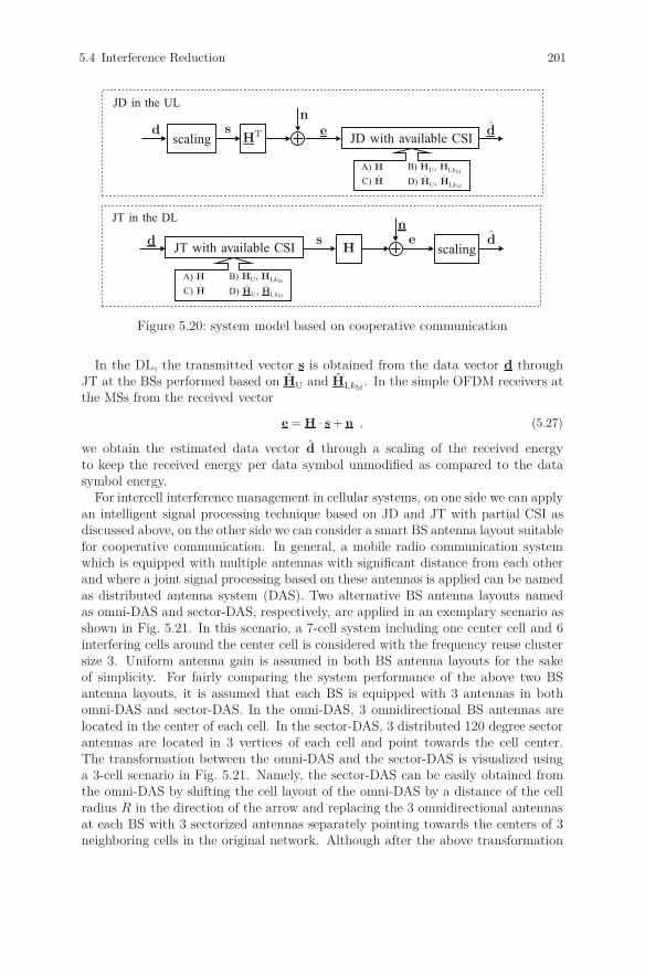
5.4 Interference Reduction 201
d
d
JD with available CSI
JT with available CSI
e
e
scaling
scaling
HT
H
n
n
s
s
A) H
A) H
B) HU, HI,kM
B) HU, HI,kM
C) H
C) H
D) HU, HI,kM
D) HU, HI,kM
d
d
JD in the UL
JT in the DL
Figure 5.20: system model based on cooperative communication
In the DL, the transmitted vector s is obtained from the data vector d throughJT at the BSs performed based on HU and HI,kM
. In the simple OFDM receivers atthe MSs from the received vector
e = H · s + n , (5.27)
we obtain the estimated data vector d through a scaling of the received energyto keep the received energy per data symbol unmodified as compared to the datasymbol energy.
For intercell interference management in cellular systems, on one side we can applyan intelligent signal processing technique based on JD and JT with partial CSI asdiscussed above, on the other side we can consider a smart BS antenna layout suitablefor cooperative communication. In general, a mobile radio communication systemwhich is equipped with multiple antennas with significant distance from each otherand where a joint signal processing based on these antennas is applied can be namedas distributed antenna system (DAS). Two alternative BS antenna layouts namedas omni-DAS and sector-DAS, respectively, are applied in an exemplary scenario asshown in Fig. 5.21. In this scenario, a 7-cell system including one center cell and 6interfering cells around the center cell is considered with the frequency reuse clustersize 3. Uniform antenna gain is assumed in both BS antenna layouts for the sakeof simplicity. For fairly comparing the system performance of the above two BSantenna layouts, it is assumed that each BS is equipped with 3 antennas in bothomni-DAS and sector-DAS. In the omni-DAS, 3 omnidirectional BS antennas arelocated in the center of each cell. In the sector-DAS, 3 distributed 120 degree sectorantennas are located in 3 vertices of each cell and point towards the cell center.The transformation between the omni-DAS and the sector-DAS is visualized usinga 3-cell scenario in Fig. 5.21. Namely, the sector-DAS can be easily obtained fromthe omni-DAS by shifting the cell layout of the omni-DAS by a distance of the cellradius R in the direction of the arrow and replacing the 3 omnidirectional antennasat each BS with 3 sectorized antennas separately pointing towards the centers of 3neighboring cells in the original network. Although after the above transformation
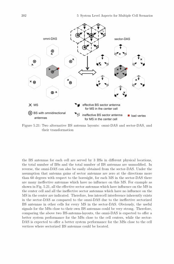
202 5 System Level Aspects for Multiple Cell Scenarios
R
MS
BS with omnidirectionalantennas
effective BS sector antennafor MS in the center cell
ineffective BS sector antennafor MS in the center cell
bad vertex
omni-DAS sector-DAS
Figure 5.21: Two alternative BS antenna layouts: omni-DAS and sector-DAS, andtheir transformation
the BS antennas for each cell are served by 3 BSs in different physical locations,the total number of BSs and the total number of BS antennas are unmodified. Inreverse, the omni-DAS can also be easily obtained from the sector-DAS. Under theassumption that antenna gains of sector antennas are zero at the directions morethan 60 degrees with respect to the boresight, for each MS in the sector-DAS thereare many ineffective antennas which have no influence on this MS. For example asshown in Fig. 5.21, all the effective sector antennas which have influence on the MS inthe center cell and all the ineffective sector antennas which have no influence on theMS in the center are indicated. Therefore, less intercell interference inherently existsin the sector-DAS as compared to the omni-DAS due to the ineffective sectorizedBS antennas in other cells for every MS in the sector-DAS. Obviously, the usefulsignals for the MSs close to their own BS antennas could be very strong. Therefore,comparing the above two BS-antenna-layouts, the omni-DAS is expected to offer abetter system performance for the MSs close to the cell centers, while the sector-DAS is expected to offer a better system performance for the MSs close to the cellvertices where sectorized BS antennas could be located.
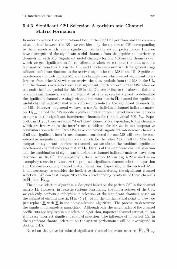
5.4 Interference Reduction 203
5.4.3 Significant CSI Selection Algorithm and Channel
Matrix Formalism
In order to reduce the computational load of the JD/JT algorithms and the commu-nication load between the BSs, we consider only the significant CSI correspondingto the channels which play a significant role in the system performance. Here wehave distinguished the significant useful channels from the significant interferencechannels for each MS. Significant useful channels for one MS are the channels overwhich we get significant useful contributions when we estimate the data symbolstransmitted from this MS in the UL, and the channels over which we generate sig-nificant useful contributions to the received signals for this MS in the DL. Significantinterference channels for one MS are the channels over which we get significant inter-ferences from other MSs when we receive the data symbols from this MS in the UL,and the channels over which we cause significant interferences to other MSs when wetransmit the data symbol for this MS in the DL. According to the above definitionsof significant channels, various mathematical criteria can be applied to determinethe significant channels. A single channel indicator matrix HU named the significantuseful channel indicator matrix is sufficient to indicate the significant channels forall MSs. However, in general we have to use KM individual channel indicator matri-ces HI,kM
named the MS specific significant interference channel indicator matricesto represent the significant interference channels for the individual MSs kM. Espe-cially, in HI,kM
, there are some “don’t care” elements corresponding to the channelswhich are irrelevant to the interference considered for MS kM in our cooperativecommunication scheme. Two MSs have compatible significant interference channelsif all the significant interference channels considered for one MS will never be con-sidered as insignificant interference channels for the other MS. If all the MSs havecompatible significant interference channels, we can obtain the combined significantinterference channel indicator matrix HI. Details of the significant channel selectionand the combination of significant interference channel indicator matrices have beendescribed in [16, 18]. For simplicity, a 3-cell sector-DAS in Fig. 5.22 is used as anexemplary scenario to visualize the proposed significant channel selection algorithmand the corresponding channel matrix formalism. Especially, in the sector-DAS itis not necessary to consider the ineffective channels during the significant channelselection. We can just assign “0”s to the corresponding positions of these channelsin HU and HI,kM
.
The above selection algorithm is designed based on the perfect CSI in the channelmatrix H. However, in realistic systems considering the imperfectness of the CSI,we can only perform a suboptimum selection of the significant channels based onthe estimated channel matrix H in (5.24). From the mathematical point of view, wejust replace H with H in the above selection algorithm. The process to determinethe significant channels is unmodified. Although only the magnitudes of the channelcoefficients are required in our selection algorithm, imperfect channel estimation canstill cause incorrect significant channel selection. The influence of imperfect CSI inthe significant channel selection on the system performance will be investigated inSection 5.4.5.
Based on the above introduced significant channel indicator matrices HU, HI,kM
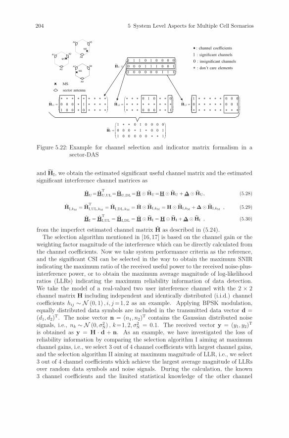
204 5 System Level Aspects for Multiple Cell Scenarios
1
0
�
�
M1
A1 A2
A3
A4 A5
A6
A7 A8
A9
M2
M3
�U
1 1 1 0 1 0 0 0 0
0 0 0 1 1 1 0 0 1
1 0 0 0 0 0 1 1 1
� �� � � �� � �
H
�I,1 0 0 0 1
1 0 0 0
� � � � � � � � �� �� � � � � � �� �� �� � � � � �
H �I,2
0 1 0 0
0 0 0 1
� � � � �� �� � � � � � � � � � �� �� �� � � � � �
H �I,3
1 0 0 0
0 0 0 1
� � � � �� �� � � � � � �� �� �� � � � � � � � � �
H
�I
1 0 1 0 0 0 0
0 0 0 1 0 0 1
1 0 0 0 0 0 1
� �� �� � � �� �� �� � �
H
MSsector antenna
: channel coefficients: significant channels: insignificant channels: don’t care elements
Figure 5.22: Example for channel selection and indicator matrix formalism in asector-DAS
and HI, we obtain the estimated significant useful channel matrix and the estimatedsignificant interference channel matrices as
HU =HT
U,UL =HU,DL =H � HU =H � HU + Δ � HU, (5.28)
HI,kM= H
T
I,UL,kM= HI,DL,kM
= H � HI,kM= H � HI,kM
+ Δ � HI,kM, (5.29)
HI = HT
I,UL = HI,DL = H � HI = H � HI + Δ � HI , (5.30)
from the imperfect estimated channel matrix H as described in (5.24).The selection algorithm mentioned in [16, 17] is based on the channel gain or the
weighting factor magnitude of the interference which can be directly calculated fromthe channel coefficients. Now we take system performance criteria as the reference,and the significant CSI can be selected in the way to obtain the maximum SNIRindicating the maximum ratio of the received useful power to the received noise-plus-interference power, or to obtain the maximum average magnitude of log-likelihoodratios (LLRs) indicating the maximum reliability information of data detection.We take the model of a real-valued two user interference channel with the 2 × 2channel matrix H including independent and identically distributed (i.i.d.) channelcoefficients hij ∼ N (0, 1) , i, j = 1, 2 as an example. Applying BPSK modulation,equally distributed data symbols are included in the transmitted data vector d =(d1, d2)
T. The noise vector n = (n1, n2)T contains the Gaussian distributed noise
signals, i.e., nk ∼ N (0, σ2N) , k=1, 2, σ2
N = 0.1. The received vector y = (y1, y2)T
is obtained as y = H · d + n. As an example, we have investigated the loss ofreliability information by comparing the selection algorithm I aiming at maximumchannel gains, i.e., we select 3 out of 4 channel coefficients with largest channel gains,and the selection algorithm II aiming at maximum magnitude of LLR, i.e., we select3 out of 4 channel coefficients which achieve the largest average magnitude of LLRsover random data symbols and noise signals. During the calculation, the known3 channel coefficients and the limited statistical knowledge of the other channel
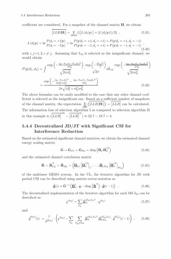
5.4 Interference Reduction 205
coefficient are considered. For a snapshot of the channel matrix H, we obtain∣∣∣LLR(H)∣∣∣ = E
{d,n}{(∣∣∣L (d1|y)
∣∣∣+ |L (d2|y)|)/2} , (5.31)
L (di|y) = lnP (di = +1|y)
P (di = −1|y)= ln
P (y|di = +1, dj = +1) + P (y|di = +1, dj = −1)
P (y|di = −1, dj = +1) + P (y|di = −1, dj = −1),
(5.32)
with i, j=1, 2, i �= j. Assuming that h12 is selected as the insignificant channel, wewould obtain
P (y|d1, d2) =∫ exp
(− (y1−h11d1−h12d2)2
2σ2N
)√
2πσ2N
·exp
(− (h12)2
2
)√
2πdh12·
exp(
− (y2−h21d1−h22d2)2
2σ2N
)√
2πσ2N
=exp
(− (y1−h11d1)2
2(d22+σ2
N)
− (y2−h21d1−h22d2)2
2σ2N
)
2π√
(d22 + σ2
N)σ2N
(5.33)
The above formulae can be easily modified to the case that any other channel coef-ficient is selected as the insignificant one. Based on a sufficient number of snapshots
of the channel matrix, the expectation E{H}
{∣∣∣LLR(H)
∣∣∣} =∣∣∣LLR
∣∣∣ can be calculated.
The information loss of selection algorithm I as compared to selection algorithm II
in this example is (∣∣∣LLR
∣∣∣(II) −∣∣∣LLR
∣∣∣(I)) ≈ 22.7 − 18.7 = 4.
5.4.4 Decentralized JD/JT with Significant CSI forInterference Reduction
Based on the estimated significant channel matrices, we obtain the estimated channelenergy scaling matrix
G = GUL = GDL = diag(HUH
∗TU
)(5.34)
and the estimated channel correlation matrix
R = RT
UL = RDL =(
HI,1
[H∗TU
]1
, . . . , HI,KM
[H∗TU
]KM
)(5.35)
of the multiuser MIMO system. In the UL, the iterative algorithm for JD withpartial CSI can be described using matrix-vector-notation as
d(i) = G−1(H∗U · e − diag
(R
T)
· d(i − 1))
. (5.36)
The decentralized implementation of the iterative algorithm for each MS kM can bedescribed as
r(kM) =∑kA
H(kM,kA)∗
U · e(kA) (5.37)
and
d(kM)
(i) =1
g(kM)·(
r(kM) −∑kA
∑k′
M�=kM
H(kM,kA)∗
U H(k′
M,kA)
I,kM· d
(k′M
)(i − 1)
), (5.38)
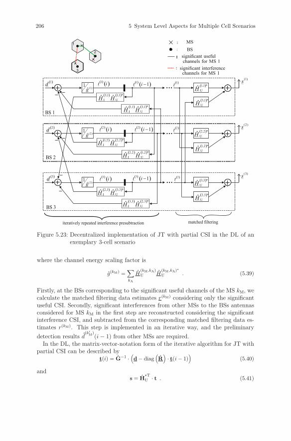
206 5 System Level Aspects for Multiple Cell Scenarios
1
2
3
:
:
:
:
iteratively repeated interference presubtraction
(1)g�
� 1d
matched filtering
BS 1
(1)s
BS 2
BS 3
� � 1,1 3,1 *
I Uˆ ˆH H
� � 3,1 1,1 *
I Uˆ ˆH H
� � 1t i � � 1
1�t i…
� 1t � 1,1 *
UH
� 3,1 *
UH
(2)g�
� 2d
(2)s
� � 1,2 2,2 *
I Uˆ ˆH H
� � 2,2 1,2 *
I Uˆ ˆH H
� � 2t i
� � 21�t i
…
� 2t � 2,2 *
UH
� 1,2 *
UH
(3)g�
� 3d
(3)s
� � 2,3 3,3 *
I Uˆ ˆH H
� � 3,3 2,3 *
I Uˆ ˆH H
� � 3t i
� � 31�t i
…
� 3t � 3,3 *
UH
� 2,3 *
UH
MSBS
significant usefulchannels for MS 1
significant interferencechannels for MS 1
Figure 5.23: Decentralized implementation of JT with partial CSI in the DL of anexemplary 3-cell scenario
where the channel energy scaling factor is
g(kM) =∑kA
H(kM,kA)U H
(kM,kA)∗
U . (5.39)
Firstly, at the BSs corresponding to the significant useful channels of the MS kM, wecalculate the matched filtering data estimates r(kM) considering only the significantuseful CSI. Secondly, significant interferences from other MSs to the BSs antennasconsidered for MS kM in the first step are reconstructed considering the significantinterference CSI, and subtracted from the corresponding matched filtering data es-timates r(kM). This step is implemented in an iterative way, and the preliminary
detection results d(k′
M)(i − 1) from other MSs are required.
In the DL, the matrix-vector-notation form of the iterative algorithm for JT withpartial CSI can be described by
t(i) = G−1 ·(d − diag
(R)
· t(i − 1))
(5.40)
ands = H
∗TU · t . (5.41)
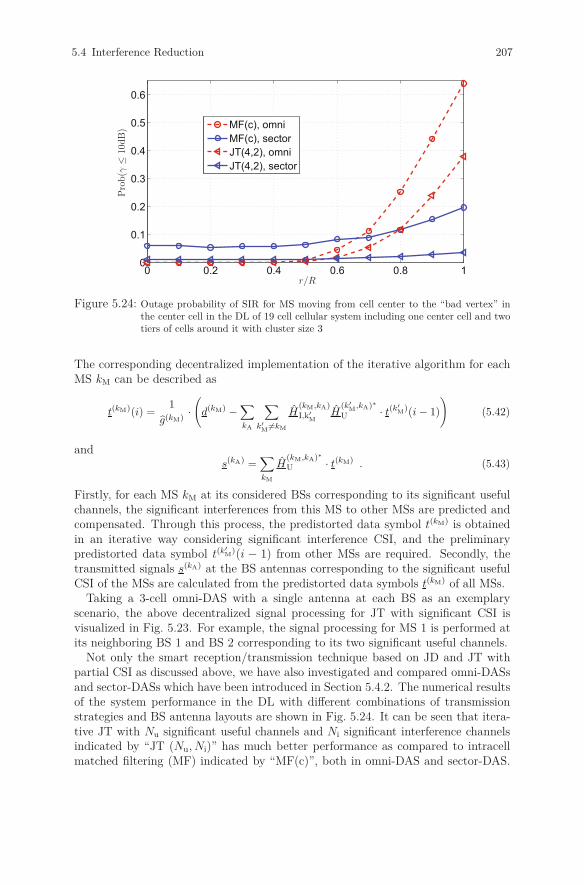
5.4 Interference Reduction 207
0 0.2 0.4 0.6 0.8 10
0.1
0.2
0.3
0.4
0.5
0.6
MF(c), omniMF(c), sectorJT(4,2), omniJT(4,2), sector
r/R
Pro
b(γ≤
10dB
)
Figure 5.24: Outage probability of SIR for MS moving from cell center to the “bad vertex” inthe center cell in the DL of 19 cell cellular system including one center cell and twotiers of cells around it with cluster size 3
The corresponding decentralized implementation of the iterative algorithm for eachMS kM can be described as
t(kM)(i) =1
g(kM)·(
d(kM) −∑kA
∑k′
M�=kM
H(kM,kA)I,k′
MH
(k′M
,kA)∗
U · t(k′M
)(i − 1)
)(5.42)
ands(kA) =
∑kM
H(kM,kA)∗
U · t(kM) . (5.43)
Firstly, for each MS kM at its considered BSs corresponding to its significant usefulchannels, the significant interferences from this MS to other MSs are predicted andcompensated. Through this process, the predistorted data symbol t(kM) is obtainedin an iterative way considering significant interference CSI, and the preliminarypredistorted data symbol t(k′
M)(i − 1) from other MSs are required. Secondly, the
transmitted signals s(kA) at the BS antennas corresponding to the significant usefulCSI of the MSs are calculated from the predistorted data symbols t(kM) of all MSs.
Taking a 3-cell omni-DAS with a single antenna at each BS as an exemplaryscenario, the above decentralized signal processing for JT with significant CSI isvisualized in Fig. 5.23. For example, the signal processing for MS 1 is performed atits neighboring BS 1 and BS 2 corresponding to its two significant useful channels.
Not only the smart reception/transmission technique based on JD and JT withpartial CSI as discussed above, we have also investigated and compared omni-DASsand sector-DASs which have been introduced in Section 5.4.2. The numerical resultsof the system performance in the DL with different combinations of transmissionstrategies and BS antenna layouts are shown in Fig. 5.24. It can be seen that itera-tive JT with Nu significant useful channels and Ni significant interference channelsindicated by “JT (Nu, Ni)” has much better performance as compared to intracellmatched filtering (MF) indicated by “MF(c)”, both in omni-DAS and sector-DAS.
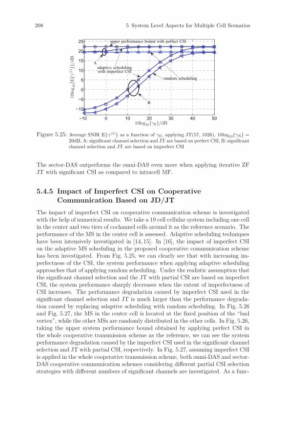
208 5 System Level Aspects for Multiple Cell Scenarios
−10 0 10 20 30 40 50
−10
−5
0
5
10
15
20
25 upper performance bound with perfect CSI
adaptive schedulingwith imperfect CSI
random scheduling
A
B
10log10{γE}/dB
10lo
g 10{E{γ
(1) }}/d
B
Figure 5.25: Average SNIR E{γ(1)} as a function of γE, applying JT(57, 1026), 10log10{γN} =20dB, A: significant channel selection and JT are based on perfect CSI, B: significantchannel selection and JT are based on imperfect CSI
The sector-DAS outperforms the omni-DAS even more when applying iterative ZFJT with significant CSI as compared to intracell MF.
5.4.5 Impact of Imperfect CSI on CooperativeCommunication Based on JD/JT
The impact of imperfect CSI on cooperative communication scheme is investigatedwith the help of numerical results. We take a 19 cell cellular system including one cellin the center and two tiers of cochannel cells around it as the reference scenario. Theperformance of the MS in the center cell is assessed. Adaptive scheduling techniqueshave been intensively investigated in [14, 15]. In [16], the impact of imperfect CSIon the adaptive MS scheduling in the proposed cooperative communication schemehas been investigated. From Fig. 5.25, we can clearly see that with increasing im-perfectness of the CSI, the system performance when applying adaptive schedulingapproaches that of applying random scheduling. Under the realistic assumption thatthe significant channel selection and the JT with partial CSI are based on imperfectCSI, the system performance sharply decreases when the extent of imperfectness ofCSI increases. The performance degradation caused by imperfect CSI used in thesignificant channel selection and JT is much larger than the performance degrada-tion caused by replacing adaptive scheduling with random scheduling. In Fig. 5.26and Fig. 5.27, the MS in the center cell is located at the fixed position of the “badvertex”, while the other MSs are randomly distributed in the other cells. In Fig. 5.26,taking the upper system performance bound obtained by applying perfect CSI inthe whole cooperative transmission scheme as the reference, we can see the systemperformance degradation caused by the imperfect CSI used in the significant channelselection and JT with partial CSI, respectively. In Fig. 5.27, assuming imperfect CSIis applied in the whole cooperative transmission scheme, both omni-DAS and sector-DAS cooperative communication schemes considering different partial CSI selectionstrategies with different numbers of significant channels are investigated. As a func-

5.4 Interference Reduction 209
−10 0 10 20 30 40
−10
−5
0
5
10
−10 0 10 20 30 40
−5
0
5
10
15
(a) omni-DAS (b) sector-DAS
upperboundupperbound
JT based on
imperfect partial CSI
imperfect partial CSI
significant channel selection
JT based onimperfect partial CSI
significant channel selectionbased on imperfect CSI
10log10{γE}/dB10log10{γE}/dB
10lo
g 10{E{γ
(1) }}/d
B
10lo
g 10{E{γ
(1) }}/d
B
Figure 5.26: Average SNIR E{γ(1)} as a function of γE, applying JT(4, 2), 10log10{γN} = 20dB
21 21.5 22 22.5 238.2
8.4
8.6
8.8
9
9.2
9.4
9.6
9.8
10
22.5 23 23.5 24 24.5
12.8
13
13.2
13.4
13.6
13.8
14
14.2
MF(c)JT(4,2)JT(4,4)JT(57,1026)
MF(c)JT(4,2)JT(4,4)JT(57,1026)
(a) omni-DAS (b) sector-DAS
10log10{γE}/dB10log10{γE}/dB
10lo
g 10{E{γ
(1) }}/d
B
10lo
g 10{E{γ
(1) }}/d
B
Figure 5.27: Average SNIR E{γ(1)} as a function of γE, 10log10{γN} = 20dB
tion of the extent of imperfectness of the CSI, we can decide how much CSI should beconsidered in the cooperative communication scheme to obtain optimum system per-formance with moderate implementation complexity. Additionally, the influence ofthe imperfectness of CSI on the advanced JD/JT algorithms, i.e., SIC in the UL andTHP in the DL with quantization, has been investigated. In Fig. 5.28 and Fig. 5.29considering the exemplary channel matrix HUL = HT
DL = (10 1 0.1; 10 2 0.1; 10 5 1),the input SNR has been adjusted in such a way that BER is always 10−3 when ap-plying different JD/JT algorithms with perfect CSI. In Fig. 5.28, ZF, SIC, ML, andoptimum MF with the ideal assumption of no multiuser interference are consideredfor JD in the receivers. In Fig. 5.29, ZF, THP, and optimum MF with the idealassumption of no multiuser interference are considered for JT in the transmitters.We can see the sensitivity of different JD/JT algorithms to the imperfectness of CSIdescribed by the variance σ2
Δ of the channel errors.

210 5 System Level Aspects for Multiple Cell Scenarios
−60 −40 −20 0 20 4010−4
10−3
10−2
10−1
100
ZFSICMLOpt. MF
10log10{σ2Δ}
BE
R
Figure 5.28: BER as a function of the extentof the imperfectness of CSI inthe UL applying JD algorithms
−60 −40 −20 0 20 4010−4
10−3
10−2
10−1
100
ZFTHPOpt. MF
10log10{σ2Δ}
BE
R
Figure 5.29: BER as a function of the extentof the imperfectness of CSI inthe DL applying JT algorithms
0 10 20 30 4010−5
10−4
10−3
10−2
ZF
suboptimum
optimum
10log10{1/σ2Δ}
BE
R
Figure 5.30: BER as a function of the extentof the perfectness of CSI with10log10{1/σ2
N} = 40dB
0 10 20 30 4010−4
10−3
10−2
ZF
suboptimum
optimum
10log10{1/σ2N}
BE
R
Figure 5.31: BER as a function of PSNR with10log10{1/σ2
Δ} = 15dB
5.4.6 Advanced Algorithm Based on Statistical Knowledge
of Imperfect CSI
Exploiting the statistical knowledge of imperfect CSI and the given alphabet S ofthe transmitted vector s, we propose an optimum detection scheme following therationale of maximum likelihood (ML) as
s = argmaxs∈S
{p(e|s, h
)}, (5.44)
where p(e|s, h
)is calculated as the marginal PDF of p
(e, h|s, h
)as
p(e|s, h
)=
∫p(e, h|s, h
)dh =
∫p (e|s, h) p(h|h)dh . (5.45)
In (5.45), p(h|h) can be calculated according to the Bayes’ theorem as
p(h|h) =p(h|h)p(h)∫p(h|h)p(h)dh
. (5.46)
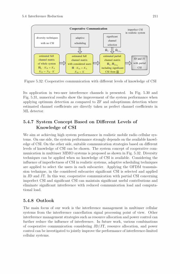
5.4 Interference Reduction 211
Cooperative Communication
diversity techniques
with no CSI
adaptive
scheduling
significantchannelselection
estimated fullchannel matrix
of whole systemHF : KM ×KA
KM = NM ·K
estimated fullchannel matrix
with considered usersH : KM ×KA
KM = K
estimated partialchannel matrix
HU, HI,kM
including significantCSI from H
JD and JT
with partial
CSI
HU HI,kM
imperfect CSIin realistic system
Figure 5.32: Cooperative communication with different levels of knowledge of CSI
Its application in two-user interference channels is presented. In Fig. 5.30 andFig. 5.31, numerical results show the improvement of the system performance whenapplying optimum detection as compared to ZF and suboptimum detection whereestimated channel coefficients are directly taken as perfect channel coefficients inML detector.
5.4.7 System Concept Based on Different Levels of
Knowledge of CSI
We aim at achieving high system performance in realistic mobile radio cellular sys-tems. On one side, the system performance strongly depends on the available knowl-edge of CSI. On the other side, suitable communication strategies based on differentlevels of knowledge of CSI can be chosen. The system concept of cooperative com-munication in multiuser MIMO systems is proposed as shown in Fig. 5.32. Diversitytechniques can be applied when no knowledge of CSI is available. Considering theinfluence of imperfectness of CSI in realistic systems, adaptive scheduling techniquesare applied to select the users in each subcarrier. Applying the OFDM transmis-sion technique, in the considered subcarrier significant CSI is selected and appliedin JD and JT. In this way, cooperative communication with partial CSI concerningimperfect CSI and significant CSI can maintain significant useful contributions andeliminate significant interference with reduced communication load and computa-tional load.
5.4.8 Outlook
The main focus of our work is the interference management in multiuser cellularsystems from the interference cancellation signal processing point of view. Otherinterference management strategies such as resource allocation and power control canfurther reduce the influence of interference. In future work, various combinationsof cooperative communication considering JD/JT, resource allocation, and powercontrol can be investigated to jointly improve the performance of interference-limitedcellular systems.
212 5 System Level Aspects for Multiple Cell Scenarios
Cooperative reception/transmission with only partial CSI is of high interest forpractical realization in future mobile radio cellular networks. Based on our con-tributions about significant CSI selection, various criteria of significant CSI can befurther investigated and applied in the realistic cellular systems. Since researchersare paying more and more attention to the cooperative communication conceptwith selected CSI [8, 9, 19–23], in future work different proposals can be compared.Further investigations could indicate which criterion for significant CSI selection ismore beneficial to system performance and which one is more beneficial to imple-mentation complexity. Combinations of different proposals and improvements of thesignificant CSI selection algorithms are expected. Some concrete design guidelinesof the selection algorithms could also be proposed.
Advanced nonlinear JD/JT algorithms, i.e., SIC with quantization in the UL andTHP in the DL, with various significant CSI selection algorithms can be furtherinvestigated with respect to analytical and numerical results in future work. Dis-tributed signal processing of these algorithms in the cooperative communicationscheme could be implemented, and its implementation complexity can be assessed.
Statistical signal processing based on limited knowledge of CSI has also been inves-tigated based on a real-valued two user interference channel model. Its applicationcan be extended to realistic multiuser cellular systems in future work.
Bibliography
[1] X. You, G. Chen, M. Chen, and X. Gao, “Toward beyond 3G: The FuTUREproject in China,” IEEE Communications Magazine, vol. 43, no. 1, pp. 38–44,Jan. 2005.
[2] K. Tachikawa, “A perspective on the evolution of mobile communications,”IEEE Communications Magazine, vol. 41, no. 1, pp. 66–73, Oct. 2003.
[3] G. J. Foschini and M. J. Gans, “On limits of wireless communications in a fadingenvironment when using multiple antennas,” Wireless Personal Commun., vol.6, pp. 311–335, Mar. 1998.
[4] E. Telatar, “Capacity of multi-antenna Gaussian channels,” European Trans-actions on Telecommunications, vol. 10, no. 6, pp. 585–595, 1999.
[5] J. G. Andrews, “Interference cancellation for cellular systems: A contemporaryoverview,” IEEE Wireless Communications, vol. 12, pp. 19–29, April 2005.
[6] R. D. J. van Nee and R. Prasad, OFDM for Wireless Multimedia Communica-tions, Artech House, Boston, 2000.
[7] T. Weber, I. Maniatis, A. Sklavos, and Y. Liu, “Joint transmission and detectionintegrated network (JOINT), a generic proposal for beyond 3G systems,” inProc. 9th International Conference on Telecommunications (ICT’02), Beijing,June 2002, vol. 3, pp. 479–483.
Bibliography 213
[8] P. Zhang, X. Tao, J. Zhang, Y. Wang, L. Li, and Y. Wang, “A vision from thefuture: Beyond 3G TDD,” IEEE Communications Magazine, vol. 43, no. 1, pp.38–44, January 2005.
[9] X. Tao, J. Xu, X. Xu, C. Tang, and P. Zhang, “Group cell FuTURE B3GTDD system,” in Proc. IEEE International Symposium on Personal, Indoorand Mobile Radio Communications (PIMRC’05).
[10] A. Klein, G. K. Kaleh, and P. W. Baier, “Zero forcing and minimum mean-square-error equalization for multiuser detection in code-division multiple accesschannels,” IEEE Transactions on Vehicular Technology, vol. 45, no. 2, pp. 276–287, May 1996.
[11] M. Meurer, P. W. Baier, T. Weber, Y. Lu, and A. Papathanassiou, “Jointtransmission: Advantageous downlink concept for CDMA mobile radio systemsusing time division duplexing,” Electronics Letters, vol. 36, no. 10, pp. 900–901,May 2000.
[12] T. Weber, A. Sklavos, and Meurer M., “Imperfect channel state information inMIMO transmission,” IEEE Transactions on Communications, vol. 54, no. 3,pp. 543–552, March 2006.
[13] S. Verdu, Multiuser Detection, University Press, Cambridge, 1998.
[14] A. Kühne and A. Klein, “Adaptive MIMO-OFDM using OSTBC with imperfectCQI feedback,” in Proc. International ITG/IEEE Workshop on Smart Antennas(WSA’08), Darmstadt, Feb. 2008.
[15] A. Kühne and A. Klein, “Throughput analysis of multi-user OFDMA-systemsusing imperfect CQI feedback and diversity techniques,” IEEE Journal onSelected Areas in Communications, vol. 26, no. 8, pp. 1440–1451, October 2008.
[16] X. Wei, T. Weber, A. Kühne, and A. Klein, “Joint transmission with imper-fect partial channel state information,” in Proc. IEEE Vehicular TechnologyConference (VTC’09-Spring), Barcelona, April 2009.
[17] X. Wei, T. Weber, A. Ahrens, and S. Deng, “Decentralized interference man-agement in mobile radio networks,” Frequenz, vol. 61, no. 11/12, pp. 259–269,2007.
[18] X. Wei, and T. Weber, “Cooperative communication with partial channel-stateinformation in multiuser MIMO systems,” AEÜ, 2010.
[19] A. Papadogiannis, H.J. Bang, D. Gesbert, and E. Hardouin, “Downlink over-head reduction for multicell cooperative processing enabled wireless networks,”in Proc. IEEE International Symposium on Personal, Indoor, Mobile RadioCommunications (PIMRC’08), Cannes, September 2008.
[20] A. Papadogiannis, D. Gesbert, and E. Hardoin, “A dynamic clustering approachin wireless networks with multi-cell cooperative processing,” in Proc. IEEEInternational Conference on Communications (ICC’08), Beijing, May 2008.

214 5 System Level Aspects for Multiple Cell Scenarios
[21] P. Marsch and G. Fettweis, “A framework for optimizing the uplink performanceof distributed antenna systems under a constrained backhaul,” in Proc. IEEEInternational Conference on Communications (ICC’07), Glasgow, June 2007.
[22] P. Marsch and G. Fettweis, “On multicell cooperative transmission in backhaul-constrained cellular systems,” Annals of Telecommunications, vol. 63, no. 5–6,pp. 253–269, June 2008.
[23] S. Khattak and G. Fettweis, “Low backhaul distributed detection strategies foran interference limited uplink cellular system,” in Proc. IEEE 67th VehicularTechnology Conference (VTC’08-Spring), Singapore, May 2008, pp. 693–697.
H. Rohling (ed.), OFDM: Concepts for Future Communication Systems, 215Signals and Communication Technology, DOI: 10.1007/978-3-642-17496-4_6,© Springer-Verlag Berlin Heidelberg 2011
6 OFDM/DMT for WirelineCommunications
With wireline, we mean digital subscriber lines as well as optical transmission. Apartfrom the general aspects of multicarrier modulation, the channel properties are verydifferent. It is thus unavoidable to go into some details of channel transfer character-istics and disturbances. In DSL, the channel characteristics are determined by thepropagation constant, the characteristic impedance, and the loop structure, further-more crosstalk from other loops and ingress (RFI, impulse noise) from outside. Incopper loops, the frequency dependent transfer function of the twisted pairs togetherwith possible reflections at splices lead to dispersion which we will also see in opticaltransmission. There, we distinguish chromatic dispersion and polarization mode dis-persion. Optical transmission especially also suffers from non-linear characteristics(Kerr effect), which does not have a counterpart in copper cables. In copper trans-mission, non-linearities are especially due to the limitations of the D/A convertersand power amplifiers, which may lead to clipping of the almost Gaussian distributedtime-domain signal of OFDM. This holds for all OFDM transmission. Other non-linearities may be due to baluns (transformers) used in DSL, but practically, theyare of minor relevance.
In the following two sections, we will study properties of the channel and specialtiesof the multicarrier transmission over twisted pairs and optical fibers. Thereafter, weconsider a new approach for impulse noise cancellation in DSL and the simulationof optical multicarrier transmission.
6.1 Discrete MultiTone (DMT) and Wireline
Channel Properties
W. Henkel, Jacobs University Bremen, Germany
This chapter describes basic properties of the wireline twister-pair channel andintroduces DMT (Discrete MultiTone), the baseband variant of OFDM. Furtherinformation can, e.g., be found in a student book project [1], or [2–5].
6.1.1 Properties of the Twisted-Pair Channel
The twisted pair (TP) cable channel is characterized by a transfer function that isincreasingly attenuating with frequency and cross-talk functions that increase withfrequency, as well. Furthermore, ingress from radio interferers (RFI), e.g., amateurradio, and impulse noise have a strong impact. In the following, we describe the
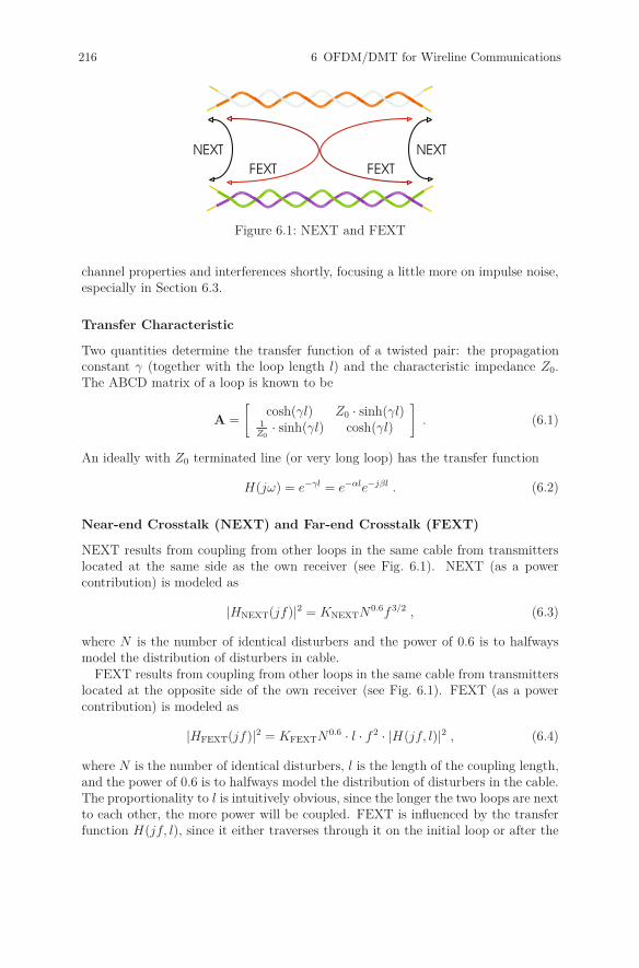
216 6 OFDM/DMT for Wireline Communications
NEXT NEXT
FEXT FEXT
Figure 6.1: NEXT and FEXT
channel properties and interferences shortly, focusing a little more on impulse noise,especially in Section 6.3.
Transfer Characteristic
Two quantities determine the transfer function of a twisted pair: the propagationconstant γ (together with the loop length l) and the characteristic impedance Z0.The ABCD matrix of a loop is known to be
A =
[cosh(γl) Z0 · sinh(γl)
1Z0
· sinh(γl) cosh(γl)
]. (6.1)
An ideally with Z0 terminated line (or very long loop) has the transfer function
H(jω) = e−γl = e−αle−jβl . (6.2)
Near-end Crosstalk (NEXT) and Far-end Crosstalk (FEXT)
NEXT results from coupling from other loops in the same cable from transmitterslocated at the same side as the own receiver (see Fig. 6.1). NEXT (as a powercontribution) is modeled as
|HNEXT(jf)|2 = KNEXTN0.6f 3/2 , (6.3)
where N is the number of identical disturbers and the power of 0.6 is to halfwaysmodel the distribution of disturbers in cable.
FEXT results from coupling from other loops in the same cable from transmitterslocated at the opposite side of the own receiver (see Fig. 6.1). FEXT (as a powercontribution) is modeled as
|HFEXT(jf)|2 = KFEXTN0.6 · l · f 2 · |H(jf, l)|2 , (6.4)
where N is the number of identical disturbers, l is the length of the coupling length,and the power of 0.6 is to halfways model the distribution of disturbers in the cable.The proportionality to l is intuitively obvious, since the longer the two loops are nextto each other, the more power will be coupled. FEXT is influenced by the transferfunction H(jf, l), since it either traverses through it on the initial loop or after the

6.1 Discrete MultiTone (DMT) and Wireline Channel Properties 217
coupling on the receiving loop. We ignore the slight differences in transfer functionson both sides which are mostly due to different twists. The so-called Equal-LevelFEXT (EL-FEXT) is defined by eliminating the length dependency and the transferfunction, i.e.,
|HEL-FEXT(jf)|2 = |HFEXT(jf)| · 1
l· 1
|H(jf, l)|2 = KFEXTN0.6 · f 2 . (6.5)
Measured NEXT and EL-FEXT functions of an 0.4-mm layered cable are shownin Fig. 6.2 and Fig. 6.3, respectively.
103 104 105 106 107−200
−180
−160
−140
−120
−100
−80
−60
−40
−20
|NE
XT|
[dB
]
frequency / Hz
Figure 6.2: Measured NEXT of an 0.4-mm layered cable
Radio-frequency Interference (RFI) and Impulse Noise
Both kinds of ingress are due to non-symmetries of the twisted pair. The pairtogether acts as an antenna, which becomes visible in the Common Mode, the averagemean of the two wires against ground. Due to non-symmetries, also in DifferentialMode, an attenuated version of the signal will be present. Non-symmetries arecharacterized by unbalance parameters like Longitudinal Conversion Loss (LCL),Transverse Conversion Loss (TCL), Longitudinal Conversion Transfer Loss (LCTL),and Transverse Conversion Transfer Loss (TCTL). We will not define them in here,instead refer to [6].
Since RFI from amateur radio stations and others are very narrow-band comparedto DSL services, they appear as a spike in the spectrum, i.e., almost a sinusoidin time domain. Countermeasures have been taken in VDSL by pulse shaping atthe transmitter and windowing at the receiver. Transmitter pulse shaping reducedegress to radio receivers, windowing at the receiver reduces ingress. Otherwise, a

218 6 OFDM/DMT for Wireline Communications
103 104 105 106 107−200
−150
−100
−50
0
50
|EL
FEX
T| [d
B/k
m]
frequency / Hz
Figure 6.3: Measured EL-FEXT of an 0.4-mm layered cable
rectangular window will lead to a stronger leakage into neighboring frequencies.Combination of neighboring carriers are also a possible measure. Also cancellationmethods based on the common mode have been proposed. These will be discussed inSection 6.3. RFI cancellation is necessary, since otherwise the desired receive signalwould be hidden in the RFI signal at the analog interface, leading to saturation ofthe A/D-converter.
Impulse noise is another disturbance that can be seen as ingress, at least whencentral offices are digitalized. In earlier times, additional strong impulse noise wascaused by relay switching in the central offices, which is not present in digitalizedcentral offices any more. Nowadays, impulse noise is only caused by electrical homeappliances, trains and trams, fluorescent tubes, ignition, lightning, and electricalmachines, especially, e.g., welding. Figure 6.4 shows an impulse, measured in aworkshop with a welding equipment and at another place caused by switching fluo-rescent tubes.The coupling mechanism for impulse noise ingress is the same as for RFI distur-bances, which means that common mode will also show a stronger interference thanthe differential mode, thereby offering possibilities for cancellation described in Sec-tion 6.3. The amplitude of impulse disturbances depends a lot on the cable infras-tructure. Especially, aerial cables carry order of magnitudes higher impulse noisethan buried cables.
In here, we shortly describe impulse-noise properties. Thorough studies on mod-eling and impulse noise generation can be found in [31–33]. The voltage follows adensity similar to Weibull, given by
fi(u) =1
240u0e|−u/u0|1/5
(6.6)
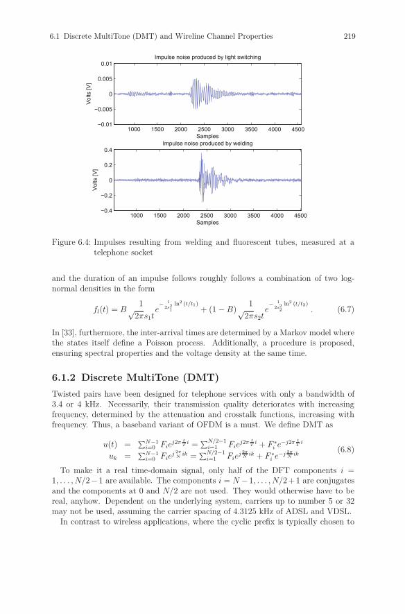
6.1 Discrete MultiTone (DMT) and Wireline Channel Properties 219
1000 1500 2000 2500 3000 3500 4000 4500−0.01
−0.005
0
0.005
0.01Impulse noise produced by light switching
Samples
Vol
ts [V
]
1000 1500 2000 2500 3000 3500 4000 4500−0.4
−0.2
0
0.2
0.4
Vol
ts [V
]
Impulse noise produced by welding
Samples
Figure 6.4: Impulses resulting from welding and fluorescent tubes, measured at atelephone socket
and the duration of an impulse follows roughly follows a combination of two log-normal densities in the form
fl(t) = B1√
2πs1te− 1
2s21
ln2 (t/t1)+ (1 − B)
1√2πs2t
e− 1
2s22
ln2 (t/t2). (6.7)
In [33], furthermore, the inter-arrival times are determined by a Markov model wherethe states itself define a Poisson process. Additionally, a procedure is proposed,ensuring spectral properties and the voltage density at the same time.
6.1.2 Discrete MultiTone (DMT)
Twisted pairs have been designed for telephone services with only a bandwidth of3.4 or 4 kHz. Necessarily, their transmission quality deteriorates with increasingfrequency, determined by the attenuation and crosstalk functions, increasing withfrequency. Thus, a baseband variant of OFDM is a must. We define DMT as
u(t) =∑N−1
i=0 Fiej2π t
Ti =
∑N/2−1i=1 Fie
j2π tT
i + F ∗i e−j2π t
Ti
uk =∑N−1
i=0 Fiej 2π
Nik =
∑N/2−1i=1 Fie
j 2πN
ik + F ∗i e−j 2π
Nik
(6.8)
To make it a real time-domain signal, only half of the DFT components i =1, . . . , N/2 −1 are available. The components i = N −1, . . . , N/2 + 1 are conjugatesand the components at 0 and N/2 are not used. They would otherwise have to bereal, anyhow. Dependent on the underlying system, carriers up to number 5 or 32may not be used, assuming the carrier spacing of 4.3125 kHz of ADSL and VDSL.
In contrast to wireless applications, where the cyclic prefix is typically chosen to
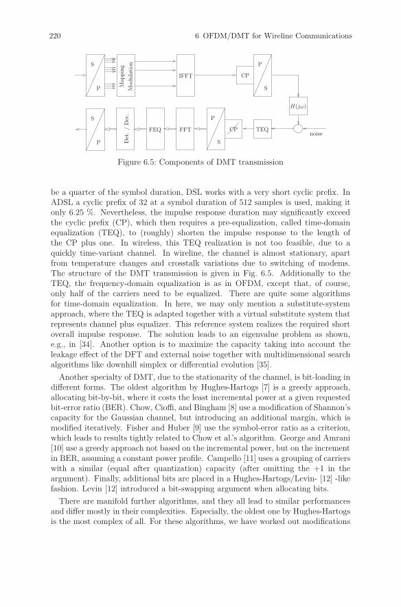
220 6 OFDM/DMT for Wireline Communications
S
P
S
P
P
S
CP
P
S
CP
noise
H(jω)
TEQFFTFEQD
et.
/D
ec.
Map
pin
g
Modula
tion
IFFT
Figure 6.5: Components of DMT transmission
be a quarter of the symbol duration, DSL works with a very short cyclic prefix. InADSL a cyclic prefix of 32 at a symbol duration of 512 samples is used, making itonly 6.25 %. Nevertheless, the impulse response duration may significantly exceedthe cyclic prefix (CP), which then requires a pre-equalization, called time-domainequalization (TEQ), to (roughly) shorten the impulse response to the length ofthe CP plus one. In wireless, this TEQ realization is not too feasible, due to aquickly time-variant channel. In wireline, the channel is almost stationary, apartfrom temperature changes and crosstalk variations due to switching of modems.The structure of the DMT transmission is given in Fig. 6.5. Additionally to theTEQ, the frequency-domain equalization is as in OFDM, except that, of course,only half of the carriers need to be equalized. There are quite some algorithmsfor time-domain equalization. In here, we may only mention a substitute-systemapproach, where the TEQ is adapted together with a virtual substitute system thatrepresents channel plus equalizer. This reference system realizes the required shortoverall impulse response. The solution leads to an eigenvalue problem as shown,e.g., in [34]. Another option is to maximize the capacity taking into account theleakage effect of the DFT and external noise together with multidimensional searchalgorithms like downhill simplex or differential evolution [35].
Another specialty of DMT, due to the stationarity of the channel, is bit-loading indifferent forms. The oldest algorithm by Hughes-Hartogs [7] is a greedy approach,allocating bit-by-bit, where it costs the least incremental power at a given requestedbit-error ratio (BER). Chow, Cioffi, and Bingham [8] use a modification of Shannon’scapacity for the Gaussian channel, but introducing an additional margin, which ismodified iteratively. Fisher and Huber [9] use the symbol-error ratio as a criterion,which leads to results tightly related to Chow et al.’s algorithm. George and Amrani[10] use a greedy approach not based on the incremental power, but on the incrementin BER, assuming a constant power profile. Campello [11] uses a grouping of carrierswith a similar (equal after quantization) capacity (after omitting the +1 in theargument). Finally, additional bits are placed in a Hughes-Hartogs/Levin- [12] -likefashion. Levin [12] introduced a bit-swapping argument when allocating bits.
There are manifold further algorithms, and they all lead to similar performancesand differ mostly in their complexities. Especially, the oldest one by Hughes-Hartogsis the most complex of all. For these algorithms, we have worked out modifications
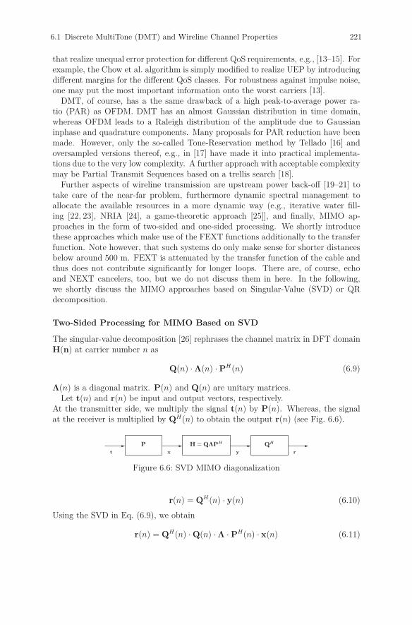
6.1 Discrete MultiTone (DMT) and Wireline Channel Properties 221
that realize unequal error protection for different QoS requirements, e.g., [13–15]. Forexample, the Chow et al. algorithm is simply modified to realize UEP by introducingdifferent margins for the different QoS classes. For robustness against impulse noise,one may put the most important information onto the worst carriers [13].
DMT, of course, has a the same drawback of a high peak-to-average power ra-tio (PAR) as OFDM. DMT has an almost Gaussian distribution in time domain,whereas OFDM leads to a Raleigh distribution of the amplitude due to Gaussianinphase and quadrature components. Many proposals for PAR reduction have beenmade. However, only the so-called Tone-Reservation method by Tellado [16] andoversampled versions thereof, e.g., in [17] have made it into practical implementa-tions due to the very low complexity. A further approach with acceptable complexitymay be Partial Transmit Sequences based on a trellis search [18].
Further aspects of wireline transmission are upstream power back-off [19–21] totake care of the near-far problem, furthermore dynamic spectral management toallocate the available resources in a more dynamic way (e.g., iterative water fill-ing [22, 23], NRIA [24], a game-theoretic approach [25]], and finally, MIMO ap-proaches in the form of two-sided and one-sided processing. We shortly introducethese approaches which make use of the FEXT functions additionally to the transferfunction. Note however, that such systems do only make sense for shorter distancesbelow around 500 m. FEXT is attenuated by the transfer function of the cable andthus does not contribute significantly for longer loops. There are, of course, echoand NEXT cancelers, too, but we do not discuss them in here. In the following,we shortly discuss the MIMO approaches based on Singular-Value (SVD) or QRdecomposition.
Two-Sided Processing for MIMO Based on SVD
The singular-value decomposition [26] rephrases the channel matrix in DFT domainH(n) at carrier number n as
Q(n) · Λ(n) · PH(n) (6.9)
Λ(n) is a diagonal matrix. P(n) and Q(n) are unitary matrices.Let t(n) and r(n) be input and output vectors, respectively.
At the transmitter side, we multiply the signal t(n) by P(n). Whereas, the signalat the receiver is multiplied by QH(n) to obtain the output r(n) (see Fig. 6.6).
t x y r
H = QΛPHP QH
Figure 6.6: SVD MIMO diagonalization
r(n) = QH(n) · y(n) (6.10)
Using the SVD in Eq. (6.9), we obtain
r(n) = QH(n) · Q(n) · Λ · PH(n) · x(n) (6.11)
222 6 OFDM/DMT for Wireline Communications
x(n) is the product of P(n) and t(n),
r(n) = QH(n) · Q(n)︸ ︷︷ ︸I
·Λ · PH(n) · P(n)︸ ︷︷ ︸I
·t(n) (6.12)
OFDM and SVD as Reed-Solomon or RS-like codes RS codes are commonlydefined as follows.
Definition 6.1.1. A Reed-Solomon (RS) code of length N and minimum Ham-ming distance dHm is a set of vectors, whose components are the values of a polyno-mial C(x) = xl · C ′(x) of degree{C ′(x)} ≤ K − 1 = N − dHm at positions zk, with zbeing an element of order N from an arbitrary number field.
c = (c0, . . . , cN−1) , ci = C(x = zi) (6.13)
wHm and dHm, the minimum Hamming weight and distance, respectively, areknown to be
wHm = min ||c||0 = dHm = N − (K − 1) = N − K + 1 . (6.14)
Since the samples are chosen to be powers of an element of order N , i.e., zk, wherez would be ej2π/N in the complex case, the equivalent description is known to be
ci = zil ·N−1∑k=0
Ckzik , i = 0, . . . , N − 1 , (6.15)
with Ck = 0 for K ≤ k ≤ N − 1, Eq. (6.15) is nothing else than an IDFT with someconsecutive DFT components unused. This means, OFDM inherently represents anRS code, when cyclically consecutive carriers are not used. In the case of DMT,these unused carrier positions need to be symmetric due to the conjugate symmetry.
Let us now compare the structures of OFDM and SVD.
OFDM: WH·channel︷ ︸︸ ︷
WΛWH ·W , (6.16)
SVD: VH · V Λ UH︸ ︷︷ ︸channel
· U . (6.17)
We observe that both make use of a pre- and post-processing by unitary matrices.IDFT and DFT diagonalize the channel Toeplitz matrix representing the convolutionwith the channel impulse response. SVD diagonalizes arbitrary channel matrices.The similarities lead to a more general concept of RS-like codes. The pre-processingmatrix of the SVD offers a code with the same Hamming distance as an RS codefor continuous and random channel matrices.
One-sided Processing for MIMO Based on QR Decomposition
Unfortunately, most of the time, we do not have the situation of a bundled connectionof only a few hundred meters where SVD would be applicable. Distances between
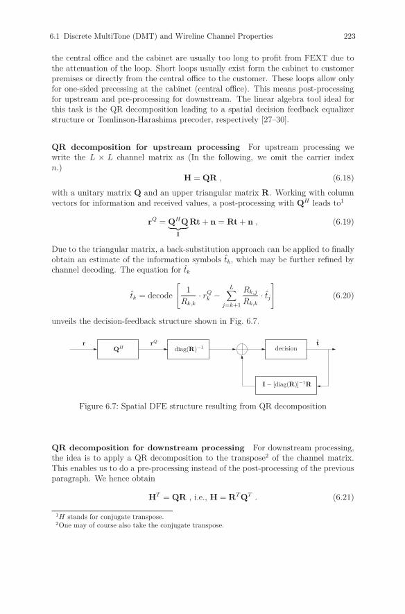
6.1 Discrete MultiTone (DMT) and Wireline Channel Properties 223
the central office and the cabinet are usually too long to profit from FEXT due tothe attenuation of the loop. Short loops usually exist form the cabinet to customerpremises or directly from the central office to the customer. These loops allow onlyfor one-sided precessing at the cabinet (central office). This means post-processingfor upstream and pre-processing for downstream. The linear algebra tool ideal forthis task is the QR decomposition leading to a spatial decision feedback equalizerstructure or Tomlinson-Harashima precoder, respectively [27–30].
QR decomposition for upstream processing For upstream processing wewrite the L × L channel matrix as (In the following, we omit the carrier indexn.)
H = QR , (6.18)
with a unitary matrix Q and an upper triangular matrix R. Working with columnvectors for information and received values, a post-processing with QH leads to1
rQ = QHQ︸ ︷︷ ︸I
Rt + n = Rt + n , (6.19)
Due to the triangular matrix, a back-substitution approach can be applied to finallyobtain an estimate of the information symbols tk, which may be further refined bychannel decoding. The equation for tk
tk = decode
⎡⎣ 1
Rk,k
· rQk −
L∑j=k+1
Rk,j
Rk,k
· tj
⎤⎦ (6.20)
unveils the decision-feedback structure shown in Fig. 6.7.
rQH
rQ
diag(R)−1
I − [diag(R)]−1R
tdecision
Figure 6.7: Spatial DFE structure resulting from QR decomposition
QR decomposition for downstream processing For downstream processing,the idea is to apply a QR decomposition to the transpose2 of the channel matrix.This enables us to do a pre-processing instead of the post-processing of the previousparagraph. We hence obtain
HT = QR , i.e., H = RT QT . (6.21)
1H stands for conjugate transpose.2One may of course also take the conjugate transpose.

224 6 OFDM/DMT for Wireline Communications
Pre-multiplying with Q∗ leads to3
rQ2 = H · Q∗ · t′ = RT · QT · Q∗︸ ︷︷ ︸=I
·t′ = RT · t′ (6.22)
Let us choose t′ ast′ = R−T · diag(RT ) · t (6.23)
The inverse of RT already ensures the desired decoupling. The diagonal matrix isadded to obtain a similar structure in the following formula as in (6.20). Equation(6.23) can equivalently be rephrased as
t′k = ΓM
⎡⎣tk −
k−1∑j=1
Rj,k
Rk,k
· t′j
⎤⎦ (6.24)
ΓM represents the modulo operation of the Tomlinson-Harashima precoding. Figure6.8 shows the precoder structure.
modulot′
Q∗
I− [diag(RT )]−1RT
t
Figure 6.8: Spatial precoder structure resulting from QR decomposition
3* means conjugate
6.2 Optical OFDM Transmission and Optical Channel Properties 225
6.2 Optical OFDM Transmission and Optical
Channel Properties
M. Mayrock, H. Haunstein, University Erlangen-Nürnberg, Germany
Commercially available systems for high bit-rate optical data transmission utilizeon-off-keying or differential phase shift keying (DPSK) and reach bit-rates up to40 Gbit/s. The transmission channel itself consists of single mode fibers exhibit-ing very low loss. In order to regenerate the power of the optical signal, opticalamplifiers, e.g., erbium doped fiber amplifiers, are placed along the link. By thismeans the optical power is increased without the need of opto-electrical signal con-version. However, optical amplifiers introduce noise, which leads to a reduction ofthe optical signal-to-noise power ratio (OSNR). Depending on the signal powers andbandwidths along with other parameters, systems can be designed for transmissionover hundreds to a couple of thousands kilometers.When transmitting over long distances various kinds of signal distortion accumulate.Chromatic Dispersion (CD) describes the effect that different frequencies travel atdifferent speeds along the optical wave-guide. Hence, pulses are broadened and fi-nally inter-symbol interference (ISI) occurs. In today’s systems CD-compensationis done with the help of dispersion compensating fibers or other optical devices likefiber gratings, which have to be adapted to the individual transmission scenario.Polarization Mode dispersion (PMD) is a further performance limiting effect. Dueto mechanical stress, imperfect fiber geometry, etc. the fiber becomes birefringent,i.e., signal contributions of orthogonal polarizations exhibit different speeds of prop-agation. The optical axes of different fiber sections are not aligned. Therefore, the“slow” and the “fast” modes of a certain piece of fiber couple into the optical axesof the next fiber section in a way which depends on their relative orientation. Thiseffect occurs all along the fiber and eventually generates a fading-channel with alarge number of echoes. There are methods for optical PMD compensation whichusually compensate for first order differential group delay. Equalization techniquesin the electrical domain could overcome this limitation. However, today’s systemsuse direct detection receivers which convert the optical signal to the electrical do-main via a non-linear operation and thus also electronic equalization shows limitedperformance.It is expected that future systems will need higher signal bandwidth leading to strictrequirements for dispersion compensation (CD and PMD). On the other hand moreand more powerful signal processing resources can be implemented in today’s inte-grated circuit fabrication processes. Therefore OFDM along with coherent detectionis a candidate for future high bit-rate optical systems.
The demand for higher bit-rates can also be accounted for using techniques whichoperate at high spectral efficiency. OFDM is interesting for such systems, as it allowsfor dense wavelength multiplexing. Moreover the modulation alphabet for individualOFDM sub-carriers can be scaled easily and thus spectral efficiency can be adaptedto given channel conditions. Recently, results of an OFDM transmission experi-ment have been published, where the authors report 5.6 bit/s/Hz spectral efficiency

226 6 OFDM/DMT for Wireline Communications
by transmitting eight times 66.8 Gbit/s over 640 km of uncompensated standardsingle-mode fiber [52]. Some modification in the set of system parameters allows forenhancement to 7.0 bit/s/Hz [53]. However, the signal-to-noise power ratio cannotbe increased to arbitrarily high values by means of increasing the optical transmitpower. This limitation is caused by the Kerr effect, which describes the variationof the refractive index of an optical wave-guide under variation of the optical signalpower. As a consequence, distorting phase modulation is caused, which is a func-tion of the signal power and finally leads to non-linear signal distortion (self phasemodulation). Furthermore the effect causes non-linear crosstalk between signals ofdifferent wavelengths and between orthogonally polarized signals.
To overcome the drawbacks of the transmission impairments and to guaranteea bit error rate (BER) < 10−16 Forward Error Correction (FEC) coding is in-evitable. In classical non-coherent direct detection receivers processing at data ratesup to 10 Gbit/s no channel capacity achieving FEC schemes were required, since ahard decision BER of already < 10−3 could be attained. So, first-generation FECschemes mainly relied on the (255, 239) Reed-Solomon (RS) code over the Galoisfield GF(256), with only 6.7% overhead. In particular, this code was recommendedby the ITU for long-haul submarine transmissions [63]. Then, the developmentof Wavelength Division Multiplexing (WDM) technology provided the impetus formoving to second-generation FEC systems, based on concatenated codes with highercoding gains [64]. Nowadays, third-generation FEC schemes based on soft-decisiondecoding have become subject of interest since stronger FEC schemes are seen asa promising way to achieve performance close to channel capacity. Therefore astraightforward approach is bit-interleaved coded modulation with iterative decod-ing (BICM-ID) , which can be considered as the most simple approach to achievehigh spectral efficiency while providing a low decoding complexity [68].
6.3 Impulse-Noise Cancellation 227
6.3 Impulse-Noise Cancellation
O. Graur, W. Henkel, Jacobs University Bremen, Germany
As previously discussed in Section 1.1, impulse noise can strongly affect trans-mission quality, occasionally even leading to DSL modem restart. In this section, acancellation method is described which relies on the strong coupling of interferenceinto Common-Mode [36].
6.3.1 Common Mode and Differential Mode
Differential-Mode (DM) signals have been the conventional approach of transmissionover copper cables. The reason behind this is that they are less susceptible tostrong interference such as impulse noise and RFI. Since DM signals appear as avoltage difference on two wires, any incident signals would couple equally, keeping thedifferential signal unchanged. Unlike DM, Common-Mode (CM) signals are takenas the arithmetic mean of the two signals measured with respect to ground, whichmakes them prone to interference. Both DM and CM signals are readily availableon the receiver side.
xDM (t) = x1(t) − x2(t) (6.25)
xCM (t) =x1(t) + x2(t)
2(6.26)
CM signals consist mainly of ingress: independent noise, a component correlatedwith the desired signal from DM, and noise correlated with the noise in DM [41].In the case of strong interference, such as in the case of impulse noise, there is astrong correlation between DM and CM signals. While the dominant componentin CM will be the impulse, this might not necessarily be the case for DM. There,impulsive noise might be buried within the rest of the signal, making the detectionless straightforward.
6.3.2 Coupling and Transfer Functions
For the rest of this section, channels were considered linear time invariant (LTI).It is also reasonable to assume that all the transmitted signals can be modeled asindependent Gaussian random variables. Since neither statistical properties, norcoupling functions were previously defined for CM, our model relies on measure-ments. For the measurements in this section, a Swiss 0.4 mm cable with 50 pairsof length 100 m was used. As Fig. 6.9 shows, measurements revealed a −50 dBattenuation of signal coupling into CM, for frequencies below 2 MHz.
Figures 6.10 and 6.11 illustrate the NEXT and FEXT coupling functions obtainedfrom measurements.
6.3.3 Common-Mode Reference-Based Canceler
The principle of impulse noise cancellation using the CM signal is illustrated inFig. 6.12.
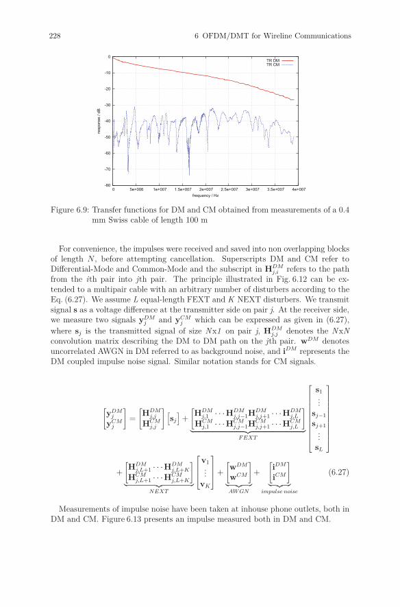
228 6 OFDM/DMT for Wireline Communications
-80
-70
-60
-50
-40
-30
-20
-10
0
0 5e+006 1e+007 1.5e+007 2e+007 2.5e+007 3e+007 3.5e+007 4e+007
resp
onse
/ dB
frequency / Hz
TR DMTR CM
Figure 6.9: Transfer functions for DM and CM obtained from measurements of a 0.4mm Swiss cable of length 100 m
For convenience, the impulses were received and saved into non overlapping blocksof length N , before attempting cancellation. Superscripts DM and CM refer toDifferential-Mode and Common-Mode and the subscript in HDM
j,i refers to the pathfrom the ith pair into jth pair. The principle illustrated in Fig. 6.12 can be ex-tended to a multipair cable with an arbitrary number of disturbers according to theEq. (6.27). We assume L equal-length FEXT and K NEXT disturbers. We transmitsignal s as a voltage difference at the transmitter side on pair j. At the receiver side,we measure two signals yDM
j and yCMj which can be expressed as given in (6.27),
where sj is the transmitted signal of size Nx1 on pair j, HDMj,j denotes the NxN
convolution matrix describing the DM to DM path on the jth pair. wDM denotesuncorrelated AWGN in DM referred to as background noise, and iDM represents theDM coupled impulse noise signal. Similar notation stands for CM signals.
[yDM
j
yCMj
]=
[HDM
j,j
HCMj,j
] [sj
]+
[HDM
j,1 · · · HDMj,j−1H
DMj,j+1 · · · HDM
j,L
HCMj,1 · · · HCM
j,j−1HCMj,j+1 · · · HCM
j,L
]︸ ︷︷ ︸
F EXT
⎡⎢⎢⎢⎢⎢⎢⎢⎢⎢⎢⎣
s1...
sj−1
sj+1...
sL
⎤⎥⎥⎥⎥⎥⎥⎥⎥⎥⎥⎦
+
[HDM
j,L+1 · · · HDMj,L+K
HCMj,L+1 · · · HCM
j,L+K
]︸ ︷︷ ︸
NEXT
⎡⎢⎢⎣
v1...
vK
⎤⎥⎥⎦ +
[wDM
wCM
]︸ ︷︷ ︸AW GN
+
[iDM
iCM
]︸ ︷︷ ︸
impulse noise
(6.27)
Measurements of impulse noise have been taken at inhouse phone outlets, both inDM and CM. Figure 6.13 presents an impulse measured both in DM and CM.
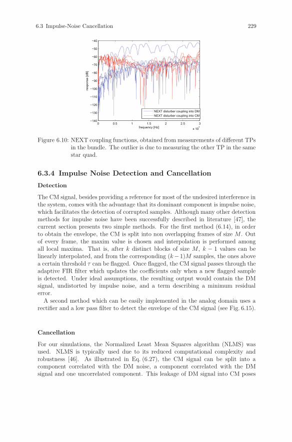
6.3 Impulse-Noise Cancellation 229
0 0.5 1 1.5 2 2.5 3
x 107
−140
−130
−120
−110
−100
−90
−80
−70
−60
−50
−40
frequency [Hz]
resp
onse
[dB
]
NEXT disturber coupling into DMNEXT disturber coupling into CM
Figure 6.10: NEXT coupling functions, obtained from measurements of different TPsin the bundle. The outlier is due to measuring the other TP in the samestar quad.
6.3.4 Impulse Noise Detection and Cancellation
Detection
The CM signal, besides providing a reference for most of the undesired interference inthe system, comes with the advantage that its dominant component is impulse noise,which facilitates the detection of corrupted samples. Although many other detectionmethods for impulse noise have been successfully described in literature [47], thecurrent section presents two simple methods. For the first method (6.14), in orderto obtain the envelope, the CM is split into non overlapping frames of size M . Outof every frame, the maxim value is chosen and interpolation is performed amongall local maxima. That is, after k distinct blocks of size M , k − 1 values can belinearly interpolated, and from the corresponding (k − 1)M samples, the ones abovea certain threshold τ can be flagged. Once flagged, the CM signal passes through theadaptive FIR filter which updates the coefficients only when a new flagged sampleis detected. Under ideal assumptions, the resulting output would contain the DMsignal, undistorted by impulse noise, and a term describing a minimum residualerror.
A second method which can be easily implemented in the analog domain uses arectifier and a low pass filter to detect the envelope of the CM signal (see Fig. 6.15).
Cancellation
For our simulations, the Normalized Least Mean Squares algorithm (NLMS) wasused. NLMS is typically used due to its reduced computational complexity androbustness [46]. As illustrated in Eq. (6.27), the CM signal can be split into acomponent correlated with the DM noise, a component correlated with the DMsignal and one uncorrelated component. This leakage of DM signal into CM poses

230 6 OFDM/DMT for Wireline Communications
0 0.5 1 1.5 2 2.5 3
x 107
−130
−120
−110
−100
−90
−80
−70
−60
−50
−40
frequency [Hz]
resp
onse
[dB
]
FEXT disturber coupling into DMFEXT disturber coupling into CM
Figure 6.11: FEXT coupling functions, obtained from measurements of different TPsin the bundle. The outliers are due to measuring adjacent TPs
∑delay
ĥ[n]
e[n]
RX/TX
RX/TX
RX/TX
x (t)1
x (t)2
xCM
xDM
DM
CMTransfer function to DM
Transfer function to CM
FEXT to DM
FEXT to CM
NEXT to DM
NEXT to CM
Figure 6.12: Coupling functions and canceler structure
the risk of canceling the useful component, which is much more likely for a high DMto CM coupling and a high SNR. One way to circumvent this problem is to updatethe filter coefficients only when the far-end transmitter is inactive [43].Uncorrelated CM in-band noise induces the possibility that it will leak to the outputof the adaptive filter, which will result in SNR loss. This undesired effect can beminimized by updating the filter coefficients only when impulse noise is detectedin CM, which is what we went for in our simulations. Crosstalk is not canceledalong with impulse noise since the total burst time is much smaller than the totaltransmission time, and the filter adaptation is performed sporadically.
6.3.5 Simulation Results
Impulse noise cancellation was investigated in the context of ADSL transmission.Coupling and transfer functions were measured for both DM and CM for a cablelength of 100 m. Length-scaling for ADSL-specific loop distances was employed usingthe method described in Chapter 1.1. Note that the same length-scaling method wasused both for DM and CM, although this might not necessarily be accurate in thecase of CM. If was used, nevertheless, since no other model for a length dependency
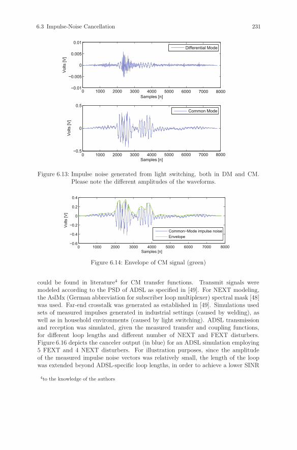
6.3 Impulse-Noise Cancellation 231
0 1000 2000 3000 4000 5000 6000 7000 8000−0.01
−0.005
0
0.005
0.01
Samples [n]
Vol
ts [V
]
0 1000 2000 3000 4000 5000 6000 7000 8000−0.5
0
0.5
Vol
ts [V
]
Samples [n]
Differential Mode
Common Mode
Figure 6.13: Impulse noise generated from light switching, both in DM and CM.Please note the different amplitudes of the waveforms.
0 1000 2000 3000 4000 5000 6000 7000 8000−0.6
−0.4
−0.2
0
0.2
0.4
Samples [n]
Vol
ts [V
]
Common−Mode impulse noiseEnvelope
Figure 6.14: Envelope of CM signal (green)
could be found in literature4 for CM transfer functions. Transmit signals weremodeled according to the PSD of ADSL as specified in [49]. For NEXT modeling,the AslMx (German abbreviation for subscriber loop multiplexer) spectral mask [48]was used. Far-end crosstalk was generated as established in [49]. Simulations usedsets of measured impulses generated in industrial settings (caused by welding), aswell as in household environments (caused by light switching). ADSL transmissionand reception was simulated, given the measured transfer and coupling functions,for different loop lengths and different number of NEXT and FEXT disturbers.Figure 6.16 depicts the canceler output (in blue) for an ADSL simulation employing5 FEXT and 4 NEXT disturbers. For illustration purposes, since the amplitudeof the measured impulse noise vectors was relatively small, the length of the loopwas extended beyond ADSL-specific loop lengths, in order to achieve a lower SINR
4to the knowledge of the authors

232 6 OFDM/DMT for Wireline Communications
0 1000 2000 3000 4000 5000 6000 7000 8000−0.6
−0.4
−0.2
0
0.2
0.4
Samples [n]
Vol
ts [V
]
Common−Mode signalEnvelope
Figure 6.15: Second method for CM envelope detection
ratio. The green line in Fig. 6.16 depicts the overall received DM signal, which iscorrupted by impulsive noise, while the black waveform illustrates the same DMsignal, impulse noise free. As expected, the canceler produces a good estimate ofthe uncorrupted DM signal but does not suppress crosstalk. The red line presentsthe ideal transmitted signal, with no interference, only attenuated by the loop. Forperfect impulse noise cancellation and no crosstalk cancellation, the blue line shouldresemble the black waveform as closely as possible, which is indeed the case.
2200 2400 2600 2800 3000 3200 3400 3600 3800 4000
−6
−4
−2
0
2
4
6
8x 10⁻³
Samples[n]
Vol
ts [V
]
Cancelled OutputImpulse + crosstalk + DM signalCrosstalk + DM signalIdeal DM signal, no crosstalk
Figure 6.16: Output of the NLMS canceler (blue). The red line represents the idealreceived signal, no crosstalk, no impulse noise, and no background noise.The black waveform denotes the sum of the ideal signal, 4 NEXT and5 FEXT disturber signals, along with background noise. The green lineillustrates the DM signal including impulse noise before cancellation.For perfect impulse noise cancellation and no crosstalk cancellation,the blue line should resemble the black signal as closely as possible.
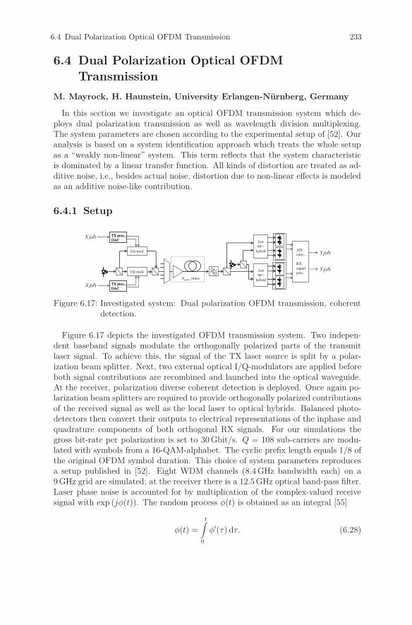
6.4 Dual Polarization Optical OFDM Transmission 233
6.4 Dual Polarization Optical OFDM
Transmission
M. Mayrock, H. Haunstein, University Erlangen-Nürnberg, Germany
In this section we investigate an optical OFDM transmission system which de-ploys dual polarization transmission as well as wavelength division multiplexing.The system parameters are chosen according to the experimental setup of [52]. Ouranalysis is based on a system identification approach which treats the whole setupas a “weakly non-linear” system. This term reflects that the system characteristicis dominated by a linear transfer function. All kinds of distortion are treated as ad-ditive noise, i.e., besides actual noise, distortion due to non-linear effects is modeledas an additive noise-like contribution.
6.4.1 Setup
Figure 6.17: Investigated system: Dual polarization OFDM transmission, coherentdetection.
Figure 6.17 depicts the investigated OFDM transmission system. Two indepen-dent baseband signals modulate the orthogonally polarized parts of the transmitlaser signal. To achieve this, the signal of the TX laser source is split by a polar-ization beam splitter. Next, two external optical I/Q-modulators are applied beforeboth signal contributions are recombined and launched into the optical waveguide.At the receiver, polarization diverse coherent detection is deployed. Once again po-larization beam splitters are required to provide orthogonally polarized contributionsof the received signal as well as the local laser to optical hybrids. Balanced photo-detectors then convert their outputs to electrical representations of the inphase andquadrature components of both orthogonal RX signals. For our simulations thegross bit-rate per polarization is set to 30 Gbit/s. Q = 108 sub-carriers are modu-lated with symbols from a 16-QAM-alphabet. The cyclic prefix length equals 1/8 ofthe original OFDM symbol duration. This choice of system parameters reproducesa setup published in [52]. Eight WDM channels (8.4 GHz bandwidth each) on a9 GHz grid are simulated; at the receiver there is a 12.5 GHz optical band-pass filter.Laser phase noise is accounted for by multiplication of the complex-valued receivesignal with exp (jφ(t)). The random process φ(t) is obtained as an integral [55]
φ(t) =
t∫0
φ′(τ) dτ. (6.28)
234 6 OFDM/DMT for Wireline Communications
Here φ′(τ) denotes zero-mean white Gaussian noise with power spectral density2πΔν. Finally, the parameter Δν describes the laser line-width, which is set to100 kHz in the sequel. The transmission link itself consisted of identical spans of stan-dard single mode fiber (length: 80 km, chromatic dispersion coefficient: 17 ps/nm/km,attenuation: 0.2 dB/km). The simulation model for the optical channel considersthe Kerr effect with the non-linear coefficient γ = 1.33/W/km [56]; polarizationdependent loss is neglected. Optical amplifiers compensate for attenuation; theirnoise-figure is assumed to be 4 dB. It should be mentioned that there are no fibersor devices for optical dispersion compensation.
6.4.2 Noise Variance Estimation
In order to determine an estimate for the maximum achievable spectral efficiency,at first the signal distortion shall be quantified. As mentioned above, the analysis isbased on a system identification approach which treats the whole setup as a “weaklynon-linear” system, i.e., the system’s characteristic is dominated by a linear transferfunction. All kinds of distortion are treated as additive noise. The transmission ofsymbol vectors [X1(d) X2(d)]T on sub-carrier d can be written as
[Y1(d)
Y2(d)
]=
[H11(d) H12(d)
H21(d) H22(d)
]·
[X1(d)
X2(d)
]+
[n1(d)
n2(d)
]. (6.29)
The samples [n1(d) n2(d)]T comprise noise which is added to the signal by opticalamplification as well as distortion due to non-linear fiber effects modeled as an ad-ditive noise-like contribution. This assumption is not valid for arbitrary points ofoperation, but reasonable for values of optical powers where we expect best trans-mission performance.After estimating the linear transfer characteristic (usually done with the help of pilotsymbols) we subtract known data symbols (either further pilot symbols or data afterdecision) which have been affected by linear distortion through the channel from thereceived symbols. Then the relative noise variance for both receive branches can bedetermined [57]:
Ni
Si
=
∑Qd=1 |ni(d)|2∑Q
d=1 |Hi1(d)X1(d) + Hi2(d)X2(d)|2 , i ∈ {1, 2} (6.30)
The summation in the nominator and denominator represents integration overthe discrete frequency spectrum. In our simulations, the per-channel optical inputpower was varied from -12 to -3 dBm. The number of fiber spans ranges from 4 to32. Based on the transmission of 100 OFDM symbols per polarization the inverseSNR of the orthogonal polarizations at the receiver is estimated according to (6.30).Figure 6.18 shows a contour plot which depicts N1/S1 in logarithmic scale. Therelative noise power increases with longer transmission distances: from less than-20 dB for short links to more than -14 dB beyond 23 spans. Furthermore the plotshows the interrelation between estimated noise variance and optical input power:For low input powers, a power increment reduces the variance of additive noise atthe receiver. At a certain power level, distortion due to fiber non-linearity comes

6.4 Dual Polarization Optical OFDM Transmission 235
Figure 6.18: Estimated relative noise power.
into play and noise power increases.
Numerous simulations have been carried out in order to quantify these observa-tions. Moreover, the influence of the launch powers of neighboring WDM channelson the noise variance has been studied. These results yield a method for separatingthe total noise variance into several contributions: Actual additive noise caused byoptical amplifiers, noise-like distortion due to self phase modulation and contribu-tions due to non-linear crosstalk between WDM channels [58].
Achievable Spectral Efficiency
According to Shannon the maximum information-rate which can be transmitted overa band-limited additive white Gaussian noise channel is
C = B · log2
(1 +
S
N
), (6.31)
where S/N and B denote the signal-to-noise power ratio and the used bandwidth.Division by B results in the achievable spectral efficiency Γ . In order to obtain anestimate for the maximum achievable spectral efficiency of the simulated OFDMsystem we determine Γ for both receive branches on sub-carrier basis
Γi(d) = log2
(1 +
E{|Hi1(d)X1(d) + Hi2(d)X2(d)|2}E{|ni(d)|2}
), i ∈ {1, 2}. (6.32)
The optical channel is assumed to be free of polarization dependent loss. Thus thecontributions of the orthogonal polarizations are added up. Furthermore we averageover the OFDM sub-carriers
Γ = η ·⎛⎝ 1
Q
Q∑d=1
Γ1(d) +1
Q
Q∑d=1
Γ2(d)
⎞⎠ . (6.33)

236 6 OFDM/DMT for Wireline Communications
Figure 6.19: Achievable spectral efficiency versus distance and launch power.
Figure 6.20: Achievable spectral efficiency vs. distance.
The coefficient η accounts for guard bands between WDM channels; in this scenariothere is a fill factor η = 8.4/9. The simulation data obtained for distances of 4 to32 spans and optical powers of -12 to -3 dBm was analyzed according to these equa-tions. The results are summarized in the contour plot in Fig. 6.19. The simulatedtransmission scenario allows for spectral efficiency of slightly more than 13 bit/s/Hzfor a distance of 4 fiber spans. For each transmission distance there is a distinctoptical power level which maximizes the SNR in the sense of a weakly non-linearsystem and at the same time yields the corresponding capacity. The extractionof the associated maximum achievable spectral efficiency versus distance is shownin Fig. 6.20. We observe a capacity decay to about 7.5 bit/s/Hz for a distance of2500 km. Due to the non-linear characteristic of the channel these results are a validestimate for the given optical setup, powers, and WDM-parameters. The channelcapacity is limited by actual additive noise along with non-linear signal distortionand non-linear cross-talk. For a comparison the diagram shows two curves which
6.4 Dual Polarization Optical OFDM Transmission 237
were obtained from approaches which consider linear AWGN channels. The investi-gated transmission system is assumed to consist of equally spaced, identical opticalamplifiers. The optical SNR (OSNR) after Nspans amplifiers is given by [59]
OSNR =Popt · λ0
G FN · h · c · Nspans · Bref
. (6.34)
Here h and c denote Planck’s constant and the speed of light, respectively. G isthe amplifiers’ gain which shall equal the loss of one fiber span. The noise figure isgiven by FN . Finally λ0 and Bref denote the reference wavelength (1550 nm) andbandwidth for noise power measurement. In optical communications usually Bref
equals 12.5 GHz. However, insertion of the actual OFDM signal bandwidth leads toan accurate SNR estimate which can be applied to Shannon’s equation. The uppercurve in Fig. 6.20 was obtained by this calculation, whereby for each transmissiondistance the optimum optical launch power found in Fig. 6.19 was inserted. It can beobserved that the numerical estimates, which consider the fiber non-linearity as anadditive noise contribution, deviate from the pure AWGN channel by approximately3 bit/s/Hz. Hence, at the optimum point of operation with respect to input power,the system still suffers from a distinct amount of distortion due to non-linear effects.An alternative way of finding a sensible value for the per-channel launch power isbased on WDM transmission parameters. Commercially availably optical amplifiersoperate in the so-called C-band which approximately ranges from 1525 to 1565 nm.Equivalently a total band-width of 5.0 THz can be used for parallel transmission.The maximum optical power typically reaches 17 dBm, e.g., used in [60]. In thecase where the total bandwidth shall be occupied by OFDM bands on a 9 GHz grid,the per-channel launch power amounts to Popt = 10.4 dBm. These considerationsare the basis for the dashed line in Fig. 6.20, obviously leading to reduced capacitycompared to the 8 channel AWGN scenario. Full occupation of the C-band resultsin penalty due to increased non-linear signal distortion. The numerical estimatesfor the achievable spectral efficiency in Fig. 6.20 exhibit a gap of approximately6 bit/s/Hz compared to the reported values of transmission experiments [52] [53].These results suggest that an increase of spectral efficiency is possible for the usedfiber links. However, first the influence of quantization noise has to be incorporatedinto the simulation model.
6.4.3 ADC/DAC Resolution
High speed devices for analog-to-digital and digital-to-analog conversion (ADC andDAC) with sampling rates beyond 20 GS/s have been demonstrated [61] as wellas the integration of four such devices, which are needed for sampling of inphaseand quadrature components of the received signals of both polarizations. At suchhigh sampling rates these devices have a more or less limited number of quantizationlevels. The authors of [61] report 6 bits resolution while state-of-the-art measurementdevices provide higher accuracy. Thus, quantization noise as well as clipping has tobe taken into consideration as performance limiting factors for high speed opticalOFDM transmission. For this purpose the simulation models of the transmitter andreceiver were extended by DAC and ADC device characteristics.
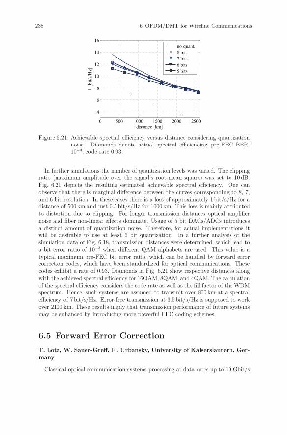
238 6 OFDM/DMT for Wireline Communications
Figure 6.21: Achievable spectral efficiency versus distance considering quantizationnoise. Diamonds denote actual spectral efficiencies; pre-FEC BER:10−3; code rate 0.93.
In further simulations the number of quantization levels was varied. The clippingratio (maximum amplitude over the signal’s root-mean-square) was set to 10 dB.Fig. 6.21 depicts the resulting estimated achievable spectral efficiency. One canobserve that there is marginal difference between the curves corresponding to 8, 7,and 6 bit resolution. In these cases there is a loss of approximately 1 bit/s/Hz for adistance of 500 km and just 0.5 bit/s/Hz for 1000 km. This loss is mainly attributedto distortion due to clipping. For longer transmission distances optical amplifiernoise and fiber non-linear effects dominate. Usage of 5 bit DACs/ADCs introducesa distinct amount of quantization noise. Therefore, for actual implementations itwill be desirable to use at least 6 bit quantization. In a further analysis of thesimulation data of Fig. 6.18, transmission distances were determined, which lead toa bit error ratio of 10−3 when different QAM alphabets are used. This value is atypical maximum pre-FEC bit error ratio, which can be handled by forward errorcorrection codes, which have been standardized for optical communications. Thesecodes exhibit a rate of 0.93. Diamonds in Fig. 6.21 show respective distances alongwith the achieved spectral efficiency for 16QAM, 8QAM, and 4QAM. The calculationof the spectral efficiency considers the code rate as well as the fill factor of the WDMspectrum. Hence, such systems are assumed to transmit over 800 km at a spectralefficiency of 7 bit/s/Hz. Error-free transmission at 3.5 bit/s/Hz is supposed to workover 2100 km. These results imply that transmission performance of future systemsmay be enhanced by introducing more powerful FEC coding schemes.
6.5 Forward Error Correction
T. Lotz, W. Sauer-Greff, R. Urbansky, University of Kaiserslautern, Ger-many
Classical optical communication systems processing at data rates up to 10 Gbit/s
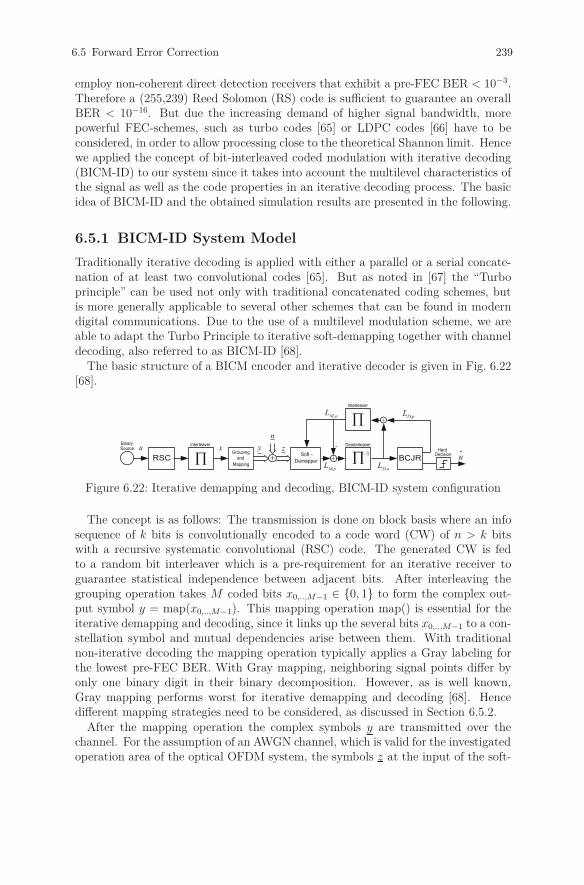
6.5 Forward Error Correction 239
employ non-coherent direct detection receivers that exhibit a pre-FEC BER < 10−3.Therefore a (255,239) Reed Solomon (RS) code is sufficient to guarantee an overallBER < 10−16. But due the increasing demand of higher signal bandwidth, morepowerful FEC-schemes, such as turbo codes [65] or LDPC codes [66] have to beconsidered, in order to allow processing close to the theoretical Shannon limit. Hencewe applied the concept of bit-interleaved coded modulation with iterative decoding(BICM-ID) to our system since it takes into account the multilevel characteristics ofthe signal as well as the code properties in an iterative decoding process. The basicidea of BICM-ID and the obtained simulation results are presented in the following.
6.5.1 BICM-ID System Model
Traditionally iterative decoding is applied with either a parallel or a serial concate-nation of at least two convolutional codes [65]. But as noted in [67] the “Turboprinciple” can be used not only with traditional concatenated coding schemes, butis more generally applicable to several other schemes that can be found in moderndigital communications. Due to the use of a multilevel modulation scheme, we areable to adapt the Turbo Principle to iterative soft-demapping together with channeldecoding, also referred to as BICM-ID [68].
The basic structure of a BICM encoder and iterative decoder is given in Fig. 6.22[68].
Figure 6.22: Iterative demapping and decoding, BICM-ID system configuration
The concept is as follows: The transmission is done on block basis where an infosequence of k bits is convolutionally encoded to a code word (CW) of n > k bitswith a recursive systematic convolutional (RSC) code. The generated CW is fedto a random bit interleaver which is a pre-requirement for an iterative receiver toguarantee statistical independence between adjacent bits. After interleaving thegrouping operation takes M coded bits x0,..,M−1 ∈ {0, 1} to form the complex out-put symbol y = map(x0,..,M−1). This mapping operation map() is essential for theiterative demapping and decoding, since it links up the several bits x0,..,M−1 to a con-stellation symbol and mutual dependencies arise between them. With traditionalnon-iterative decoding the mapping operation typically applies a Gray labeling forthe lowest pre-FEC BER. With Gray mapping, neighboring signal points differ byonly one binary digit in their binary decomposition. However, as is well known,Gray mapping performs worst for iterative demapping and decoding [68]. Hencedifferent mapping strategies need to be considered, as discussed in Section 6.5.2.
After the mapping operation the complex symbols y are transmitted over thechannel. For the assumption of an AWGN channel, which is valid for the investigatedoperation area of the optical OFDM system, the symbols z at the input of the soft-
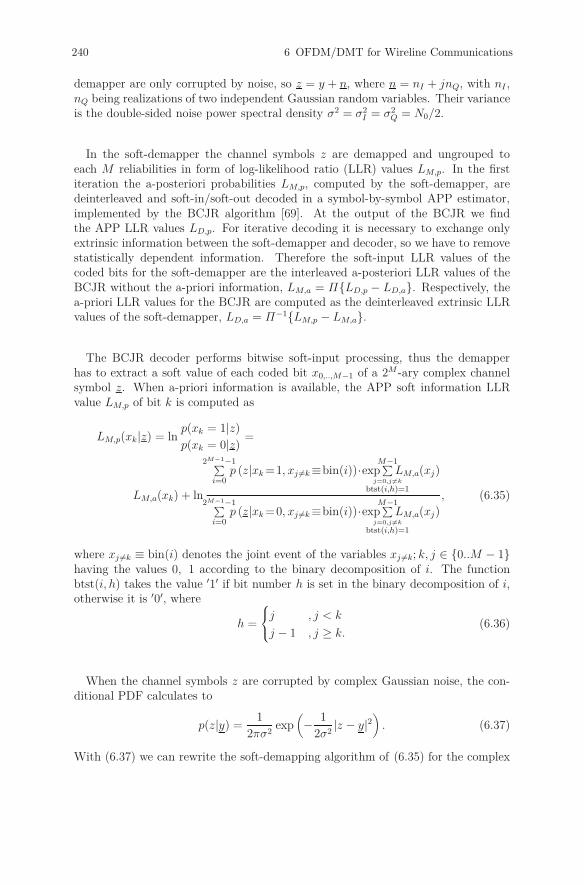
240 6 OFDM/DMT for Wireline Communications
demapper are only corrupted by noise, so z = y + n, where n = nI + jnQ, with nI ,nQ being realizations of two independent Gaussian random variables. Their varianceis the double-sided noise power spectral density σ2 = σ2
I = σ2Q = N0/2.
In the soft-demapper the channel symbols z are demapped and ungrouped toeach M reliabilities in form of log-likelihood ratio (LLR) values LM,p. In the firstiteration the a-posteriori probabilities LM,p, computed by the soft-demapper, aredeinterleaved and soft-in/soft-out decoded in a symbol-by-symbol APP estimator,implemented by the BCJR algorithm [69]. At the output of the BCJR we findthe APP LLR values LD,p. For iterative decoding it is necessary to exchange onlyextrinsic information between the soft-demapper and decoder, so we have to removestatistically dependent information. Therefore the soft-input LLR values of thecoded bits for the soft-demapper are the interleaved a-posteriori LLR values of theBCJR without the a-priori information, LM,a = Π{LD,p − LD,a}. Respectively, thea-priori LLR values for the BCJR are computed as the deinterleaved extrinsic LLRvalues of the soft-demapper, LD,a = Π−1{LM,p − LM,a}.
The BCJR decoder performs bitwise soft-input processing, thus the demapperhas to extract a soft value of each coded bit x0,..,M−1 of a 2M -ary complex channelsymbol z. When a-priori information is available, the APP soft information LLRvalue LM,p of bit k is computed as
LM,p(xk|z) = lnp(xk = 1|z)
p(xk = 0|z)=
LM,a(xk) + ln
2M−1−1∑i=0
p (z|xk =1, xj �=k ≡bin(i))·expM−1∑
j=0,j �=k
btst(i,h)=1
LM,a(xj)
2M−1−1∑i=0
p (z|xk =0, xj �=k ≡bin(i))·expM−1∑
j=0,j �=k
btst(i,h)=1
LM,a(xj)
, (6.35)
where xj �=k ≡ bin(i) denotes the joint event of the variables xj �=k; k, j ∈ {0..M − 1}having the values 0, 1 according to the binary decomposition of i. The functionbtst(i, h) takes the value ′1′ if bit number h is set in the binary decomposition of i,otherwise it is ′0′, where
h =
⎧⎨⎩j , j < k
j − 1 , j ≥ k.(6.36)
When the channel symbols z are corrupted by complex Gaussian noise, the con-ditional PDF calculates to
p(z|y) =1
2πσ2exp
(− 1
2σ2|z − y|2
). (6.37)
With (6.37) we can rewrite the soft-demapping algorithm of (6.35) for the complex

6.5 Forward Error Correction 241
AWGN channel as
LM,p(xk|z) = LM,a(xk) + ln
2M−1−1∑i=0
exp
⎡⎢⎣− 1
2σ2 |z − yk,(1,i)
|2 +M−1∑
j=0,j �=k
btst(i,h)=1
LM,a(xj)
⎤⎥⎦
2M−1−1∑i=0
exp
⎡⎢⎣− 1
2σ2 |z − yk,(0,i)
|2 +M−1∑
j=0,j �=k
btst(i,h)=1
LM,a(xj)
⎤⎥⎦
, (6.38)
where yk,(1,i)
= map(xk=1,xj �=k ≡bin(i)) and yk,(0,i)
= map(xk=0,xj �=k ≡bin(i)), j ∈{0..M − 1}.
6.5.2 Influence of the Applied Mapping
As noted before, the choice of the mapping is crucial to achieve a good performanceof BICM-ID. If Gray mapping is applied the initial BER performance is acceptable,but the performance of the iteration loop is inferior, whereas for, e.g., an anti-Graymapping its convergence behavior can be significantly improved for the price of aworse initial BER. So, for anti-Gray mapping a quite high SNR is required to reachthe so called “turbo cliff”, which is the required SNR at which the decoding processstarts to deliver an iteration gain.
However, systems applying the Turbo Principle are known to run into a certainerror floor. Hence, if a lower BER is intended outer coding is indispensable. Whenthe necessary pre-FEC BER of the outer FEC scheme is known, it is possible tooptimize the BICM-ID system to reach that specific error region by applying anirregular modulation at a lower SNR compared to the case of applying either a pureGray or a pure anti-Gray mapping. So the symbols within a CW are mapped to aratio of α according to Gray and to a ratio 1 − α according to anti-Gray,
α =NGray
NGray + NAnti−Gray
(6.39)
with N{Gray,Anti−Gray} denoting the number of symbols within a CW owning a Grayor anti-Gray mapping, respectively [62].
6.5.3 Simulations on the Performance of Coded OFDM
In this section BICM-ID is optimized according to the properties of the opticalOFDM system. The investigated coded OFDM transmission system with polariza-tion multiplexing is depicted in Fig. 6.23.
Outer coding is implemented by the (255,239) RS-Code code of rate RRS = 0.937over the Galois field GF(256), specified by the ITU in [63]. This particular codehas the property to guarantee a BER < 10−16 when the RS decoder input BER is< 10−3.
To enhance the error correction capabilities of the transmission system, innercoding is performed with a BICM encoder. So, the RS-encoder output sequence u isconvolutionally encoded with a RSC encoder of memory 5 and punctured to result
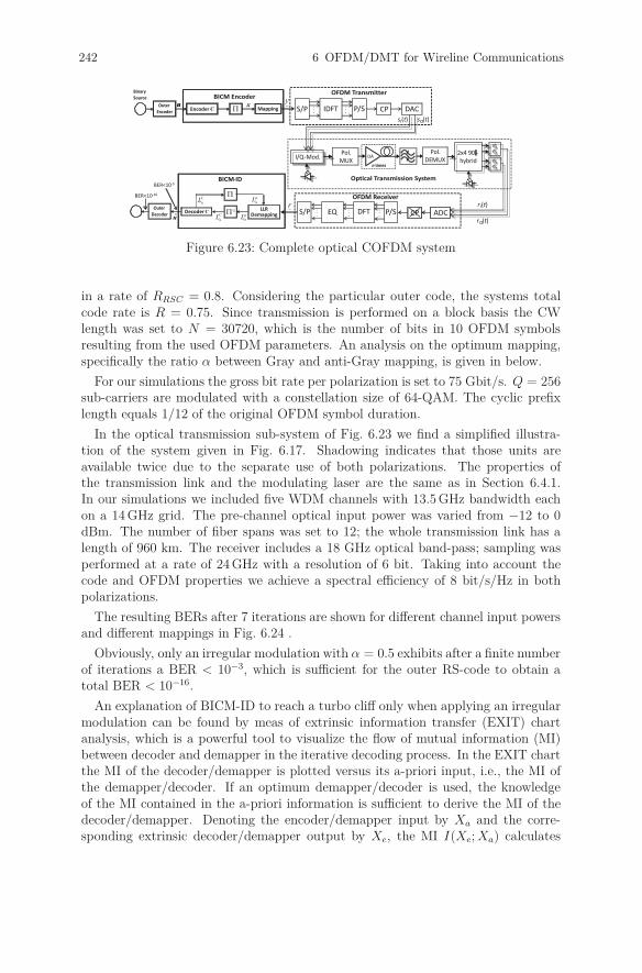
242 6 OFDM/DMT for Wireline Communications
Figure 6.23: Complete optical COFDM system
in a rate of RRSC = 0.8. Considering the particular outer code, the systems totalcode rate is R = 0.75. Since transmission is performed on a block basis the CWlength was set to N = 30720, which is the number of bits in 10 OFDM symbolsresulting from the used OFDM parameters. An analysis on the optimum mapping,specifically the ratio α between Gray and anti-Gray mapping, is given in below.
For our simulations the gross bit rate per polarization is set to 75 Gbit/s. Q = 256sub-carriers are modulated with a constellation size of 64-QAM. The cyclic prefixlength equals 1/12 of the original OFDM symbol duration.
In the optical transmission sub-system of Fig. 6.23 we find a simplified illustra-tion of the system given in Fig. 6.17. Shadowing indicates that those units areavailable twice due to the separate use of both polarizations. The properties ofthe transmission link and the modulating laser are the same as in Section 6.4.1.In our simulations we included five WDM channels with 13.5 GHz bandwidth eachon a 14 GHz grid. The pre-channel optical input power was varied from −12 to 0dBm. The number of fiber spans was set to 12; the whole transmission link has alength of 960 km. The receiver includes a 18 GHz optical band-pass; sampling wasperformed at a rate of 24 GHz with a resolution of 6 bit. Taking into account thecode and OFDM properties we achieve a spectral efficiency of 8 bit/s/Hz in bothpolarizations.
The resulting BERs after 7 iterations are shown for different channel input powersand different mappings in Fig. 6.24 .
Obviously, only an irregular modulation with α = 0.5 exhibits after a finite numberof iterations a BER < 10−3, which is sufficient for the outer RS-code to obtain atotal BER < 10−16.
An explanation of BICM-ID to reach a turbo cliff only when applying an irregularmodulation can be found by meas of extrinsic information transfer (EXIT) chartanalysis, which is a powerful tool to visualize the flow of mutual information (MI)between decoder and demapper in the iterative decoding process. In the EXIT chartthe MI of the decoder/demapper is plotted versus its a-priori input, i.e., the MI ofthe demapper/decoder. If an optimum demapper/decoder is used, the knowledgeof the MI contained in the a-priori information is sufficient to derive the MI of thedecoder/demapper. Denoting the encoder/demapper input by Xa and the corre-sponding extrinsic decoder/demapper output by Xe, the MI I(Xe; Xa) calculates
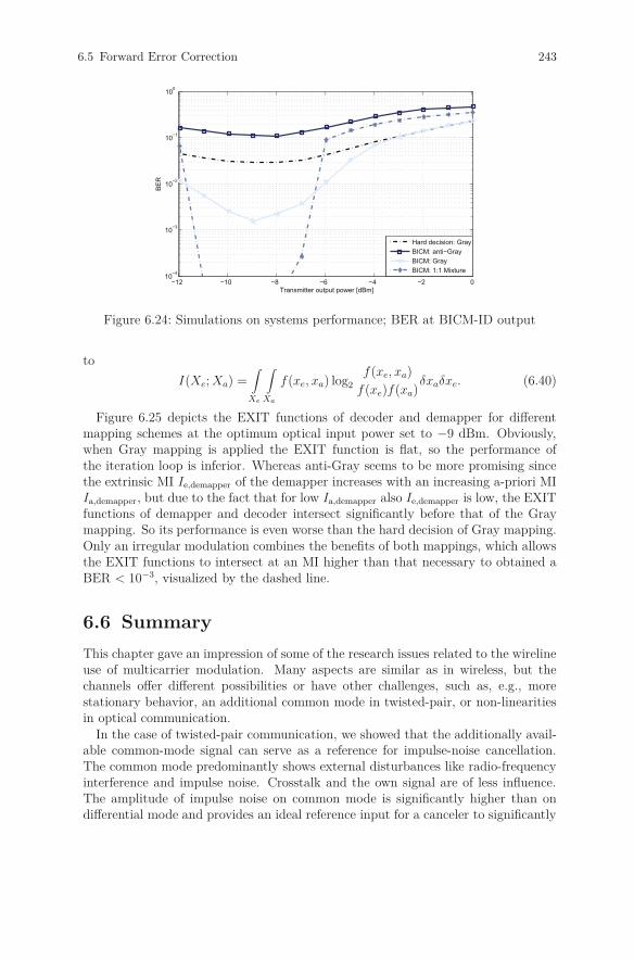
6.5 Forward Error Correction 243
−12 −10 −8 −6 −4 −2 010−4
10−3
10−2
10−1
100
Transmitter output power [dBm]
BE
R
Hard decision: GrayBICM: anti−GrayBICM: GrayBICM: 1:1 Mixture
Figure 6.24: Simulations on systems performance; BER at BICM-ID output
to
I(Xe; Xa) =∫
Xe
∫Xa
f (xe, xa) log2
f(xe, xa)
f (xe)f(xa)δxaδxe. (6.40)
Figure 6.25 depicts the EXIT functions of decoder and demapper for differentmapping schemes at the optimum optical input power set to −9 dBm. Obviously,when Gray mapping is applied the EXIT function is flat, so the performance ofthe iteration loop is inferior. Whereas anti-Gray seems to be more promising sincethe extrinsic MI Ie,demapper of the demapper increases with an increasing a-priori MIIa,demapper, but due to the fact that for low Ia,demapper also Ie,demapper is low, the EXITfunctions of demapper and decoder intersect significantly before that of the Graymapping. So its performance is even worse than the hard decision of Gray mapping.Only an irregular modulation combines the benefits of both mappings, which allowsthe EXIT functions to intersect at an MI higher than that necessary to obtained aBER < 10−3, visualized by the dashed line.
6.6 Summary
This chapter gave an impression of some of the research issues related to the wirelineuse of multicarrier modulation. Many aspects are similar as in wireless, but thechannels offer different possibilities or have other challenges, such as, e.g., morestationary behavior, an additional common mode in twisted-pair, or non-linearitiesin optical communication.
In the case of twisted-pair communication, we showed that the additionally avail-able common-mode signal can serve as a reference for impulse-noise cancellation.The common mode predominantly shows external disturbances like radio-frequencyinterference and impulse noise. Crosstalk and the own signal are of less influence.The amplitude of impulse noise on common mode is significantly higher than ondifferential mode and provides an ideal reference input for a canceler to significantly

244 6 OFDM/DMT for Wireline Communications
0 0.2 0.4 0.6 0.8 10.5
0.55
0.6
0.65
0.7
0.75
0.8
0.85
0.9
0.95
1
Ia,demapper, Ie,decoder
I e,de
map
per, I
a,de
code
r
Soft−Demapper: anti−GraySoft−Demapper: GraySoft−Demapper: 1:1 MixtureDecoder
BER = 10−3
Figure 6.25: EXIT functions of decoder and soft-demapper for different mappings atoptical input power of -9 dBm.
reduce impulse-noise in differential mode.In optics, we were aiming at a maximum achievable spectral efficiency, which is
limited by amplifier noise and non-linear fiber effects causing signal distortion andnon-linear crosstalk between WDM channels. A weakly non-linear approach wasapplied which treats all these kinds of distortion as additive noise. Based on noisevariance determination, estimates for the maximum achievable spectral efficiency areobtained, which amount to a range of 13 bit/s/Hz to 7.5 bit/s/Hz for distances from320 km up to 2500 km. Realistic ADC/DAC characteristics turned out to slightlyreduce the achievable spectral efficiency for short to medium distances. For long-haul transmission, quantization noise is not dominating. Forward error correctioncodes standardized for optical transmission leave a gap of approximately 4 bit/s/Hzto the estimated upper bound.To overcome this gap, we adapted the principle of an iterative decoding scheme,namely BICM-ID, to our system. The obtained results for the investigated opticalOFDM system promise to reach a spectral efficiency of 8 bit/s/Hz for a 960 km fiberlink. However, we expect to enhance the performance beyond that by applying evenmore powerful FEC schemes, such as multi-level codes or LDPC codes.
Bibliography
[1] http://trsys.faculty.jacobs-university.de/files/DSL_book_project.pdf
[2] T. Starr, J.M. Cioffi, and P.J. Silverman, Understanding Digital Subscriber LineTechnology, Prentice Hall, 1998.
[3] J.M. Cioffi, T. Starr, M. Sorbara, DSL Advances, Prentice Hall, 2002.

Bibliography 245
[4] W.Y. Chen, “Dsl: Simulation Techniques and Standards Development for DigitalSubscriber Line Systems,” Macmillan Technology Series, 1998.
[5] P. Golden, H. Debieu, K. Jacobsen, edts., Fundamentals of DSL Technology,Auerbach Publications, Boca Raton, FL, USA, 2006.
[6] ETSI TM 6 contribution, Luleå, Sweden, June 22-26, 1998, 970p02r3.
[7] D. Hughes-Hartogs, D., Ensemble Modem Structure for Imperfect TransmissionMedia, U.S. Patents, Nos. 4,679,227 (July 1987); 4,731,816 (March, 1988); and4,833,706 (May 1989).
[8] P.S. Chow, J.M. Cioffi, J.A.C. Bingham, “A practical discrete multitonetransceiver loading algorithm for data transmission over spectrally shaped chan-nels,” IEEE Transactions on Communications, Vol. 43, No. 234, pp. 773-775,Feb-Mar-Apr 1995.
[9] R.F.H. Fischer, J.B. Huber, “A New Loading Algorithm for Discrete MultitoneTransmission,” proc. Globecom 1996, Vol. 1, Nov. 18-22, 1996, pp. 724-728.
[10] Y. George, O. Amrani, “Bit loading algorithms for OFDM,” proc. InternationalSymposium on Information Theory (ISIT) 2004, p. 391, June 27 - July 2, 2004.2004 Page(s):391 - 391
[11] J. Campello, “A Practical Bit Loading for DMT,” proc. ICC 1999, Vancouver,Vol. 2, pp. 801-805, June 1999.
[12] H.E. Levin, “A complete and optimal data allocation method for practical dis-crete multitone systems,” GLOBECOM 2001, San Antonio, TX, USA, Vol. 1,pp. 369-374, Nov. 25-29, 2001.
[13] W. Henkel and K. Hassan, “OFDM (DMT) Bit and Power Loading for UnequalError Protection,” OFDM-Workshop 2006, Hamburg, Aug. 30-31, 2006.
[14] K. Hassan and W. Henkel, “UEP with Adaptive Multilevel Embedded Modula-tion for MIMO-OFDM Systems,” OFDM-Workshop 2008, Hamburg, Aug. 27-28,2008.
[15] F. Yu, A. Willson, “A DMT Transceiver Loading Algorithm for Data Transmis-sion with Unequal Priority over Band-limited Channels,” proc. Signals, Systems,and Computers, 1999, Pacific Grove, CA, USA, Vol. 1, pp. 685-689, Oct. 24-27,1999.
[16] J. Tellado, Peak-to-Average Power Reduction for Multicarrier Modulation,Ph.D. thesis, Stanford University, Sept. 1999.
[17] W. Henkel, V. Zrno, “PAR Reduction Revisited: An Extension to Tellado’sMethod,” 6th International OFDM-Workshop, Hamburg, Sept. 18-19, 2001.
246 6 OFDM/DMT for Wireline Communications
[18] W. Henkel, V. Azis, “Partial Transmit Sequences and Trellis Shaping,” 5thInternational ITG Conference on Source and Channel Coding (SCC), Erlangen,January 14-16, 2004.
[19] K.S. Jacobsen, “Methods of Upstream Power Backoff on Very High-Speed Digi-tal Subscriber Lines,” IEEE Communications Magazine, pp. 210-216, March 2001
[20] B. Wiese, K.S. Jacobsen, “Use of the Reference Noise Method Bounds thePerformance Loss Due to Upstream Power Backoff,” IEEE JSAC, Vol. 20, No. 5,pp. 1075-1084, June 2002.
[21] S. Schelstraete, “Define Upstream Power Backoff for VDSL,” IEEE JSAC,Vol. 20, No. 5, pp. 1064-1074, June 2002.
[22] S.T. Chung and J.M. Cioffi, “Rate and Power Control in a Two-user MulticarrierChannel with no Coordination: the Optimal Scheme vs. a Suboptimal Method,”IEEE Transactions on Communications, Vol. 51, No. 11, pp. 1768–2003, Nov2003.
[23] S.T. Chung, S.J. Kim, J. Lee, and J.M. Cioffi, “A Game-theoretic Approach toPower Allocation in Frequency Selective Gaussian Interference Channels,” in Proc.of the IEEE International Symposium on Information Theory, ISIT, Yokohama,Japan, p. 316. June-July 2003,
[24] D. Statovci, Adaptive Resource Allocation for Multi-User Digital SubscriberLines, Ph.D. thesis, Vienna University of Technology, July 2005.
[25] A. Leshem and E. Zehavi, “Game Theory and the Frequency Selective Inter-ference Channel,” IEEE Signal Processing Magazine, Vol. 26, No. 5, pp. 28-40,September 2009.
[26] G. Tauböck, W. Henkel, “MIMO Systems in the Subscriber-Line Network,” 5thInternational OFDM Workshop, Hamburg, Sept. 12-13, 2000.
[27] G. Ginis, J.M. Cioffi, “Vectored Transmission for Digital Subscriber Line Sys-tems,” IEEE JSAC, Vol. 20, No. 5, pp. 1085-1104, June 2002.
[28] G. Ginis, J.M. Cioffi, “A multi-user precoding scheme achieving crosstalk can-cellation with application to DSL systems,” proc. Thirty-Fourth Asilomar Con-ference on Signals, Systems and Computers, 2000, Vol. 2, pp. 1627-1631, Oct. 29- Nov. 1, 2000.
[29] G. Ginis, J.M. Cioffi, “On the relation between V-BLAST and the GDFE,”IEEE Communications Letters, Vol. 5, No. 9, pp. 364-366, Sept. 2001.
[30] R.F.H. Fischer, C. Windpassinger, A. Lampe, and J.B. Huber, “Space-TimeTransmission using Tomlinson-Harashima Precoding,” ITG Fachbericht, 2002.
[31] W. Henkel, T. Kessler, “A Wideband Impulsive Noise Survey in the GermanTelephone Network: Statistical Description and Modeling,” AEÜ, Vol. 48, No. 6,pp. 277-288, Nov. 1994.
Bibliography 247
[32] W. Henkel, T. Kessler, H.Y. Chung, “Coded 64-CAP ADSL in an Impulse-NoiseEnvironment – Modeling of Impulse Noise and First Simulation Results,” IEEEJSAC, Vol. 13, No. 9, Dec. 1995, pp. 1611-1621.
[33] I. Mann, S. McLaughlin, W. Henkel, R. Kirkby, and T. Kessler, “Impulse Gen-eration wich Appropriate Amplitude, Length, Inter-arrival, and Spectral Charac-teristics,” IEEE JSAC, Vol. 20, No. 5, pp. 901-912, June, 2002.
[34] M. van Bladel and M. Moeneclaey, “Time-domain equalization for multicar-rier communication,” in Proc. Communication Theory Mini-Conf. (GLOBECOM1995), pp. 167-171, Singapore, Nov. 13–17, 1995.
[35] W. Henkel and T. Kessler, “Maximizing the Channel Capacity of Multicar-rier Transmission by Suitable Adaptation of the Time-Domain Equalizer,” IEEETransactions on Communications, Vol. 48, No. 12, pp. 2000-2004, Dec. 2000.
[36] W. Henkel and O. Graur, “Impulse Noise Cancellation based on the Common-Mode Signal,” proc. Sarnoff Symposium, Princeton, NJ, USA, Apr. 12 -14, 2010,Princeton, NJ, USA.
[37] W. Henkel, T. Kessler,“A Wideband Impulsive Noise Survey in the GermanTelephone Network: Statistical Description and Modeling ,” AEÜ, Vol. 48, No. 6,pp. 277-288, Nov./Dec. 1994.
[38] W. Henkel, T. Kessler, H.Y. Chung,“A Wideband Impulse-Noise Survey onSubscriber Lines and Inter-Office Trunks: Modeling and Simulation,” Globe-com/CTMC ’95, Singapore, Nov. 13-17, 1995.
[39] I. Mann, S. McLaughlin, W. Henkel, R. Kirkby, T. Kessler,“Impulse Generationwith Appropriate Amplitude, Length, Inter-arrival, and Spectral Characteristics,”IEEE J. Select. Area Commun., Vol. 20, No. 6, pp. 901-912, June 2002.
[40] G. Ginis, C. Peng,“Alien Crosstalk Cancellation for Multipair Digital SubscriberLine Systems,” EURASIP Journal on Applied Signal Processing, Vol. 2006, 2006.
[41] T. Magesacher, P. Ödling, P. O. Börjesson and T. Nordström,“Exploiting theCommon-Mode Signal in xDSL,” European Signal Processing Conference 2004,Vienna, Austria, September 2004.
[42] T. Magesacher, P. Ödling, P. O. Börjesson,“Analysis of Adaptive InterferenceCancellation Using Common-Mode Information in Wireline Communications,”EURASIP Journal on Applied Signal Processing, Vol. 2007, 2007.
[43] T. Magesacher, P. Ödling, P. O. Börjesson,“Adaptive Interference Cancella-tion using Common-Mode Information in DSL,” Proc. European Signal ProcessingConference 2005, Antalya, Turkey, September 2005.
[44] P. Ödling, P. O. Börjesson, T. Magesacher and T. Nordström,“An Approachto Analog Mitigation of RFI,” IEEE J. Select. Area Commun., Vol. 20, No. 5,pp. 974-986, June, 2002.
248 6 OFDM/DMT for Wireline Communications
[45] S. Haykin, Adaptive Filter Theory, Englewood Cliffs, Prentice Hall, 1986.
[46] B. Widrow, J. R. Glover, J. M. Mccool, J. Kaunitz, C. S. Williams, R. H. Hean,J. R. Zeidler, E. Dong, and R. C. Goodlin,“An Adaptive Noise Cancelling: Prin-ciples and Applications,” Proc. IEEE, Vol. 63, No. 12, pp. 1692-1716, December,1975.
[47] T. Chen, C. Tsai, T. Y. Chen,“An Intelligent Impulse Noise Detection Methodby Adaptive Subband-Based Multi-State Median Filtering,” Second InternationalConference on Innovative Computing, Information and Control, ICICIC 2007,5-7 September, 2007.
[48] W. Henkel, T. Kessler,“Simulation of ADSL over ISDN on German SubscriberLines,” IEEE Communications Letters, Vol. 1, No. 5, pp. 124-126, September1997.
[49] Draft ITU-T Recommendation G.996.1,“Test Procedures for Digital SubscriberLine (DSL) Transceivers,” International Telecommunication Union.
[50] T. Nordström,“A model for an Austrian PE04 cable,” ETSI STC TM6, Sophia-Antipolis, France, September 29 — October 3, 2003.
[51] L. Heylen, J. Musson,“Cable Models predict physically impossible Behaviourin Time Domain,” ETSI TM6 Meeting, Amsterdam, Netherlands November 29— December 1, 1999.
[52] H. Takahashi, A. A. Amin, S. L. Jansen, I. Morita, H. Tanaka, “8x66.8-Gbit/sCoherent PDM-OFDM Transmission over 640 km of SSMF at 5.6-bit/s/Hz Spec-tral Efficiency,” Proc. ECOC 2008, Th.3.E.4, Sept.2008.
[53] H. Takahashi, A. A. Amin, S. L. Jansen, I. Morita, H. Tanaka, “DWDM Trans-missi on with 7.0-bit/s/Hz Spectral Efficiency using 8x65.1-Gbit/s CoherentPDM-OFDM Signals,” Proc. OFC, PDPB7, March 2009.
[54] R.-J. Essiambre, G. Foschini, P. Winzer, G. Kramer, “Capacity Limits of Fiber-Optic Communication Systems,” Proc. OFC, OThL1, March 2009.
[55] L. Kazovsky, S. Benedetto, A. Willner, Optical Fiber Communication Systems,Artech House, 1996.
[56] G. P. Agrawal, Nonlinear Fiber Optics, Academic Press, 2nd edition, 1995.
[57] M. Mayrock, H. Haunstein, “Optical Monitoring for Non-Linearity Identifica-tion in CO-OFDM Transmission Systems,” Proc. OFC, JThA58, Feb. 2008.
[58] M. Mayrock, H. Haunstein, “Monitoring of Linear and Non-linear Signal Dis-tortion in Coherent Optical OFDM Transmission,” IEEE Journal of LightwaveTechnology, vol. 27, no. 16, pp. 3560-3566, Aug. 2009.
[59] I.P. Kaminow, T.L. Koch, Optical Fiber Telecommunications IIIB, AcademicPress, 1997.

Bibliography 249
[60] X. Zhou, J. Yu, M.-F. Huang, Y. Shao, T. Wang, P. Magill, M. Cvijetic,L. Nelson, M. Birk, G. Zhang, S. Ten, H.B. Matthew, S.K. Mishra, “32Tb/s(320x114Gb/s) PDM-R Z-8QAM transmission over 580km of SMF-28 ultra-low-loss fiber,” Proc. OFC, PD PB4, March 2009.
[61] B. Beggs, “Microelectronics Advancements to Support New Modulation For-mats and DSP Techniques,” Proc. OFC, OThE4, March 2009.
[62] T. Lotz, W. Sauer-Greff, R. Urbansky, “Iterative Demapping with Non-Euclidean Metric for Optical COFDM Systems,” 14th International OFDM-Workshop, Hamburg, Germany, Sep. 2009
[63] “Interfaces for the Optical Transport Network,” Telecommunication Standard-ization Sector, International Telecommunication Union, G. 709, Mar. 2003.
[64] “Forward error correction for high bit rate DWDM submarine systems,”Telecommunication Standardization Sector, International TelecommunicationUnion, G.975.1, February 2004.
[65] C. Berrou , A. Glavieux, P. Thitimajshima, “Near Shannon limit error-correcting coding and decoding: Turbo-codes,” Proc. ICC , Geneva, Switzerland,pp. 1064-1070, May 1993.
[66] R. G. Gallager, “Low-Density Parity-Check Codes”, IRE Trans. on Info. The-ory, Vol. IT-8, pp. 21-28, Jan. 1962.
[67] J. Hagenauer, “The Turbo Principle: Tutorial Introduction and State of theArt”, Symposium on Turbo Codes, Brest, France, September 1997.
[68] S. ten Brink, J. Speidel, R.-H. Yan, “Iterative Demapping and Decoding forMultilevel Modulation,” in IEEE GLOBECOM, Sydney, Australia, Vol. 1, pp.579-584, July 1998.
[69] L. Bahl, J. Cocke, F Jelinek, J. Raviv, “Optimal Decoding of Linear Codesfor Minimizing Symbol Error Rate,” IEEE Trans. Inform. Theory, vol. 20, pp.284-287, Mar. 1974.

251
Index
�-essential support, 112adaptive MIMO transmission, 99adaptive modulation, 90, 98ADC/DAC resolution, 237automatic modulation classification, 103
basisbiorthogonal, 109dual, 109orthonormal, 109Riesz, 110
BC, see broadcast channelBCJR algorithm, 240beamforming, 147, 100, 181, 193
low-complex, 150BICM, see bit-interleaved coded
modulationbiorthogonal, see basis, biorthogonalbit allocation table, 102bit loading, 90bit-interleaved coded modulation, 85, 116
with iterative decoding (BICM-ID), 226,239
bit-loading, 98broadcast channel, 83broadcast techniques, 122
cancellation, 227, 229channel
capacity, 98coding, 84correlation, 22
distance, 24inter-site, 23, 24intra-site, 23link level, 23
system layout level, 23
estimation, 39impulse response, 2matrix, 110, 112–113modeling, 31
deterministic, 18double-directional, 16geometry-based, 15, 21stochastic, 20
multidimensional, 15operator, 109–111parameters
high-resolution estimation, 17large-scale, 21
sounding, 17state information, 85time varying, 110time-invariant, 110transfer function, 3, 16, 169
Chromatic Dispersion (CD), 225coexistence, 133coherence bandwidth, 3coherence time, 3common mode, 227compact support, 111cooperative downlink, 24Costa precoding, 83cross-layer adaptation, 176, 180crosstalk, 216CSI
imperfect, 142partial, 199
cyclic prefix, 5, 110
differential mode, 227diffraction
geometrical theory, 18Digital Radio Mondiale (DRM), 54

252 Index
Discrete Fourier transform, 8inverse, 8
Discrete MultiTone (DMT), 98, 215,219
DMT, see Discrete MultiTone (DMT)dual, see basis, dualdual polarization transmission, 233dynamic frequency selection, 169dynamic rate adaptation, 172
effective SNR, 100eigenmode transmission, 99eigenvalue update, 123EXIT charts, 129exponential effective SNR mapping, 100extrinsic information transfer (EXIT), 54
fading, 54Feichtinger algebra, 111FEXT, 216Forward Error Correction (FEC), 226,
238, 239frequency diversity, 142Gabor system, 109
generic link model, 115generic model, 118graph-based soft data and channel
estimation, 40
Huffman coding, 103
impulse noise, 217, 227, 228information-rate, 235intelligent transportation networks, 156interference
alignment, 192inter-carrier (ICI), 5intercarrier (ICI), 110intersymbol (ISI), 4, 81, 110reduction, 199
joint detection (JD), 199joint transmission (JT), 199
Kerr effect, 226, 234
large system analysis, 152Laser phase noise, 233lattice constants, 109LDPC codes, 54line-of-sight propagation, 111, 112link adaptation, 165link efficiency, 175
loading algorithm, 85log-likelihood ratio (LLR), 240low-density parity-check (LDPC), 54LTE, 115
MAC, see multiple access channelmapping, 239matrix representation of OFDM signals,
158maximum ratio combining (MRC), 54Medium Access Control (MAC)
protocols, 146MIMO, see Multiple-Input Multiple-Out-
put(MIMO)
MIMO channel, 70, 81MIMO OFDM, 70, 81MIMO transmission, 81, 82
multipoint-to-point, 81point-to-multipoint, 81point-to-point, 81
minimum rate requirements, 123modulation, 81
multicarrier, 81singlecarrier, 81
modulation and coding scheme, 171multi-carrier cyclic antenna frequency
spreading, 48multi-path propagation, 2multi-path structure, 17, 21multi-user interference, 81multilevel modulation, 239multiple access, 10multiple access channel, 82multiple link scenario, 165Multiple-Input Multiple-Output (MIMO),
99, 221, 222multiuser diversity, 142mutual information (MI), 55
NEXT, 216nonlinear detection, 36nonlinear distortions, 33
optical channel, 225optical OFDM transmission, 233orthogonality, 6orthonormal, 109, see basis, orthonormaloverlay system, 133
packet transmission efficiency, 175PAR, 69
worst-case, 69PAR reduction, 69
Index 253
downlink Transmission, 73MIMO transmission, 71
PAR reduction scheme, 70clipping and filtering, 70constellation expansion, 70partial transmit sequences, 70, 71Reed–Solomon code, 72selected mapping, 70, 71shaping techniques, 70side information, 74Simplex code, 72successive scheme, 72tone reservation, 70
parallel decoding, 116partial transmit sequences, 70peak-to-average power ratio, see PARpeak-to-average power reduction, 34,
see PAR reductionper antenna rate control, 100physical link parameters, 169polarization dependent loss, 234Polarization Mode dispersion (PMD), 225power constraint, 83power loading, 172pre-equalizer, 136predistortion, 34, 35pricing algorithms, 193propagation scenario, 16, 17, 19, 21PTS, see partial transmit sequencespulse shaping, 109, 111
QR decomposition, 222
radar, 156joint radar and communication system,
156radio channel, 2
time-variant, 136rate allocation, 128rate region, 82, 83ray-tracing, 136RayTracing, 157Reed Solomon (RS) code, 239Reed-Solomon (RS) code, 222relaying, 24RFI, 217Riesz, see basis, Riesz
RS code, see Reed-Solomon (RS) code
selected mapping, 70self-organizing resource allocation, 182signaling overhead, 102significant interference channel, 203significant useful channel, 203singular-value decomposition, 221SLM, see selected mappingsoft impulse shaping, 136soft-demapping, 239, 240Space DivisionMultiple Access (SDMA),
146space-frequency coding, 100spatial grouping, 147spatial multiplexing, 100spreading, 47
function, 111successive bit loading, 92Successive Encoding Successive Allocation
Method (SESAM), 150sum-rate maximization, 123SVD, 221
TCM, see trellis-coded modulationTHP, see Tomlinson–Harashima precoding,
see Tomlinson–Harashimaprecoding
time varying, see channel, time varyingtime-invariant, see channel, time-invariantTomlinson–Harashima precoding, 73, 83transmit power control, 170trellis-coded modulation, 85Turbo
codes (TC), 54diversity, 55equalization, 61, 128principle, 239, 241
twisted pairs, 215
uplink-downlink duality, 82, 83utility-based scheduling, 186
VBLAST, 100
Weyl-Heisenberg system, 109Wiener filter, 58