Embed Size (px)
Citation preview

Signal versus Noise in Eukaryotic Chemotaxis
Herbert LevineUCSD-CTBP (an NSF-supported PFC)
With: Wouter-Jan Rappel, W. Loomis, D. Fuller (Biology)W. Chen, B. Hu, M. Buenemann, D. Shao (CTBP)
Outline:• Experiments on chemotactic response in Dictyostelium• Signal versus noise in gradient sensing• Nonlinear amplification via signal transduction• Cell motility mechanics

Cells know where to go
QuickTime™ and aH.264 decompressor
are needed to see this picture.
Wild-type leukocyte response to fin wound
Matthias et al(2006)

Close-up view of chemotaxis
Dictybase Website http://dictybase.org/index.html
Cell moves about one cell diameter per minuteDecision-making maintains flexibility
QuickTime™ and aYUV420 codec decompressor
are needed to see this picture.

Cell migration in a gradient
QuickTime™ and a decompressor
are needed to see this picture.
cAMP gradient
flow rate 640 m/s
1h real time = 8 sec movie
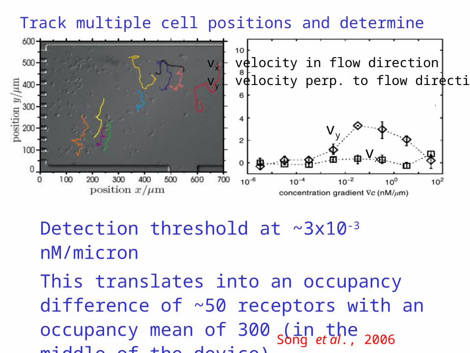
Track multiple cell positions and determine chemotactic velocity
vy
vx
Detection threshold at ~3x10⁻³ nM/micron
This translates into an occupancy difference of ~50 receptors with an occupancy mean of 300 (in the middle of the device)
Song et al., 2006
vx: velocity in flow directionvy: velocity perp. to flow direction

Subcellular polarity markers
Receptors
Occupancy
PI3K
PTEN
RAC
Myosin
Starting with the work of Parent and Devreotes, response can be tracked by subcellular markers
•Uniform CAR1 receptor•Lipid modification via PI3K•F-actin at the front (via RAC)•Myosin at the rear
These allow for the measurement of the kinetics of the gradient sensing step

New uncaging technique
From C. Beta, PotsdamUncaged cAMP in a flow creates well-defined excitationAnal Chem. (2007)
QuickTime™ and a decompressor
are needed to see this picture.

Questions for theory
• Can one predict macroscopic measures of cell motility given the space-time course of an applied signal and (possibly) the cell history– Cell speed, directional persistence, chemotactic index
– Not just averages, but also distributions
– Not just wild-type, but also mutant strains
• We are nowhere near this goal– New pathways still being discovered
– Many unresolved questions as to mechanisms

Sensing Noise• Sensing is done roughly 50K receptors, each with a binding constant of 30nM.• One can calculate directly the amount of information available to the cell regarding the external gradient angle
where y is vector of occupancies whose probability distribution is a Gaussian with mean and variance
For small gradients, M = p(y,)log
p(y,)p(y)p()∫
i =Ci
Ci + K
σ i2 =
KCi
Ni (Ci + K )2
M ~NK
4C0
R∇CC0 +K
⎛
⎝⎜
⎞
⎠⎟
2
Note: Result is in bits of information
Diffusive correlations are negligible

Sensing model

Sensing Noise• Sensing is done roughly 50K receptors, each with a binding constant of 30nM.• One can calculate directly the amount of information available to the cell regarding the external gradient angle
where y is vector of occupancies whose probability distribution is a Gaussian with mean and variance
For small gradients,
M = p(y,)logp(y,)
p(y)p()∫
i =Ci
Ci + K
σ i2 =
KCi
Ni (Ci + K )2
M ~NK
4C0
R∇CC0 +K
⎛
⎝⎜
⎞
⎠⎟
2
Note: Result is in bits of information
Diffusive correlations are negligible

Compare to experiment
• We can directly compare this number to the information about the gradient indicated by the actual cell motion
C.I. = 0.556
100
Movement up gradient
5% gradient
C.I. = ± 0.04
100
no gradient
Fuller, Chen et al, PNAS (2010)

In shallow gradients the E + I mutual information is limited by the external mutual information (receptor occupancy).
E + I mutual information decreesat higher concentrations due toan increase in internal noise.
We also analyzed theinstantaneous angle of thecells in the devices.
Result: The cell operates at the sensor noise limit for smallgradients and concentrations; eventually limited by other noiseand/or processing losses

Phenomenological approach
• We can compare the results of the experiment to a phenomenological
model where extra noise is added to the sensing noise dφdt
=−β(ρ)sin(φ−ψ)+η0
ρ= gradient strengthψ= noisy estimate of gradient directionη=extrinsic noise (due to bare motility)
From this, we can directly calculate the stationary distribution of angles of cell motion; generalization of circular normal distribution (Hu et al, PRE 2009)

Aside: Cooperative receptors
• Receptor cooperativity can lower the noise for concentrations close to Kd
Sets bound on cell size for spatial sensing (Hu et al, PRL 2010)

Signaling models
• Can we go beyond this phenomenological approach to discuss actual gradient sensing process
• We will focus on a gradient sensing approach, which tries to explain how external signals can get amplified to the level of decisions

LEGI -first conceptual model
Local activation and global inhibitionexplains adaptation to global stimulusversus steady gradient response
• Successes– Reasonable match to data (esp. in Latrunculin treated cells)
• Shortcomings– Gives linear amplification (x3 in Lat)- no polarity formation!– Inconsistent with data (Postma et al) on post-adaptation structures– Local activation cannot really work in the presence of noise (later)
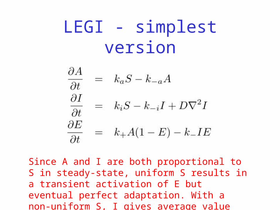
LEGI - simplest version
Since A and I are both proportional to S in steady-state, uniform S results in a transient activation of E but eventual perfect adaptation. With a non-uniform S, I gives average value and A remains local - pattern in the effector E

LEGI
Local activation and global inhibitionexplains adaptation to global stimulusversus steady gradient response
• Successes– Reasonable match to data (esp. in Latrunculin treated cells)– Can be extended to model more biological detail
• Shortcomings– Gives linear amplification (x3 in Lat)- no polarity formation!– Inconsistent with data (Postma et al) on spontaneous structures

Can we post-amplify?
•To amplify the internal gradient, we need to set a threshold for some process
•Small gap between front and back at a variable PIP3 level - in simplest model, would need some sort of cell-by-cell learning
•Amplification possible via molecular depletion (Nossal et al) - but, this leads to timescale issues
Would fall apart without absolutely perfect adaptation
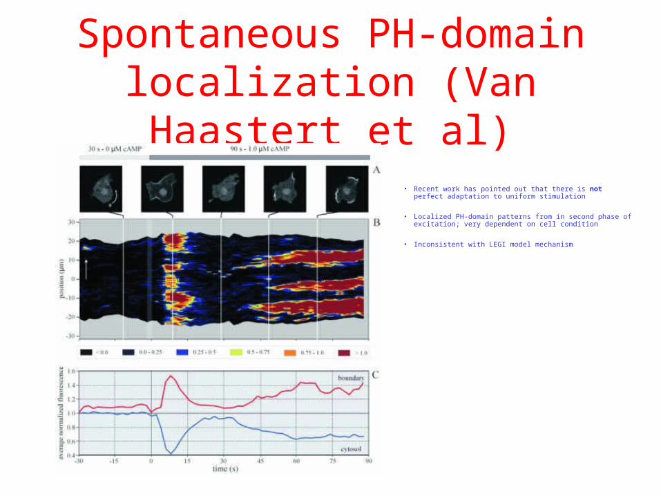
Spontaneous PH-domain localization (Van Haastert et al)
• Recent work has pointed out that there is not perfect adaptation to uniform stimulation
• Localized PH-domain patterns from in second phase of excitation; very dependent on cell condition
• Inconsistent with LEGI model mechanism

A decision-making module
• Inhibitor acts via removing the activator. • We balance the system such that the amount of (diffusing) inhibitor created by
the signal roughly equals the amount of (local) activator - operating guess - trimeric G protein subumits
• With gradient: surplus activator in front (follows external signal), surplus inhibitor in back (no response at all!)
• Can work this out analytically in a simplified 1d geometry
Membrane-bound activatorDiffusing inhibitor

New model includes a membrane-bound activator, A, a cytosolic inhibitor, B, along with its membrane-bound version Bm
€
∂A
∂t= kaS − k− a A − ks ABm on membrane
∂Bm
∂t= kbB − k− bBm − ks ABm on membrane
∂B
∂t= D∇2B in cytosol
∂B
∂n= kaS − kbB boundary condition
Balanced inactivation model (PNAS 2006)
€
A f
Ab
=kaks
k−ak−b
(Δc)2
c
Note balance inA and B production
Front to back ratio is large if decay rates are small

Experiment vs theory
Janetopoulos et al 2004Background subtraction
Levine, Kessler and Rappel, 2006Simplest prediction: no change in PH-CRAC at back membrane

Initial symmetric response - becomes asymmetric after 10 secs
Janetopoulos et al PNAS (2004)Xu et al (2005)(NB Latrunculin)
System maintains ability to respond to changing gradients
Firtel lab UCSD

Mutual Information after processing
Preliminary results
• Model captures high concentration saturation
• Possible need for new mechanism at low C
• Can be compared to other models (ultrasensitive LEGI)
Background c = 5nm
Motility Aspects
The cell needs to take the input sensing data and make a decision, based on cellular signaling networks, which way to go. After this decision, the cell needs to organize itself so as to generate the forces and shape changes needed for the actual motion.
In the remainder of this talk, I will briefly mention our very new efforts to try to understand some of these mechanical aspects of directed cell motility.

Cell in a microfluidic device with chemoattractant gradient, variable vertical height.Most of the cell in focal plane: no bleaching issuesVisualize Ras*, an upstream signaling component
Monica Skoge, Loomis lab
Phenomenological model of motility (Inbal)

Model has two components:
• A “biochemical” model which is able to produce regions of elevated concentration of a component (patches).
• A mechanical model which deforms the cell based on the patch concentration
QuickTime™ and aH.264 decompressor
are needed to see this picture.
Hecht et al submitted
SIMPLE PHENOMENOLOGICAL MODEL
Tip-splitting; expt. versus simulation

Traction Microscopy
• Data from del Alamo (Lasheras/Firtel) 2008
QuickTime™ and aSorenson Video 3 decompressorare needed to see this picture.
Pole forces at front and rear of cell
Motility cycle - Protrusion, contraction

Adhesion sites
•Uchida and Yumura showed that that there were specific adhesion sites connecting the actin cytoskeleton to the substratum
•These sites come and go as the cell goes through its motility cycle
•Our model focuses on the forces generated by these points, modeled as breakable springs
Note: Dicty does not have specialized focal adhesions

Dictyostelium cells have (non-specific) adhesion sites
Vertically restricted Dictyostelium cell in gradient, with actin marker limE at the top (green) and at the bottom surface (red)

Modeling assumptions
• We focus on the part of the cell in contact• The motility cycle consists of contraction (a-c)
and then protrusion (c-e)• Contraction is assumed to happen at constant
speed, up to a fixed percentage (accomplished by Myosin motors)
• During contraction, sites can detach if the force is too high
(Buenemann et al Biophys J. 2010)

Adhesive springs
• Uniform contraction implemented incrementally
• Compute forces (rigid or elastic substratum)
• After each time-step, adjust cell c.o.m/angle to give zero net force
• Allow springs to break at rate
• After contraction is done, assume that the cell protrusion carries the cell forward such that its back is at the last adhesive site.
• Measure traction forces, cell speeds etc as a function of the parameters
koff ,i =k0
off exp(KsΔ |rxi −
rx0,i |/kT )

Modeling assumptions
• We focus on the part of the cell in contact• The motility cycle consists of contraction (a-c) and
then protrusion (c-e)• Contraction is assumed to happen at constant speed,
up to a fixed percentage (accomplished by Myosin motors)
• During contraction, sites can detach if the force is too high

Results
Displacementmax ~ .2microns
Stress fieldPeak ~ 40 Pascal
Agrees reasonably well with traction microscopy data

Cell velocity
Speed is relatively insensitive to the values of the adhesion parameters, within a significant range
Agrees roughly with some mutant experiments; different than mammalian cells.
But, this model does not have any serious treatment of protrusion To go further, we need to start thinking about cell deformations and actin-based propulsion

Deforming Cells
• We have begun the task of constructing a model of the mechanics of deformation
• Our approach is based on a phase-field formulation of the membrane energy coupled to actin-polymerization forces
E =σ ds+ c2
κ 2∫∫ ds+ MA
2(A−A0 )
2 •Surface energy•Bending energy•Area constraintd 2x
ε2(∇φ)2 +G(φ)
⎛
⎝⎜
⎞
⎠⎟∫
d2xε
ε∇2φ−G(φ)ε
⎛
⎝⎜
⎞
⎠⎟∫2
surface
bending
This formulation can allow us to reproduce results on theequilibrium shapes of vesicles

Preliminary results
• To get to moving cells, we need to add in external forces on the protruding front, generated by actin polymerization onto a network attached by adhesions to the substrate; do this is in an ad-hoc fashion
Look at simple cells•Keratocytes•Steady motion•Velocity related to aspect ratio
•But, we need to improve our modeling approach

Summary
• Chemotactic response requires a sophisticated biophysics approach– Models are necessarily spatially-extended
– Noise is not negligible
– Cell geometry is complex and changeable
• We have used a variety of methods to look initially at the signaling and more recently at the mechanics
• Eventually, we will understand how it really works!