Embed Size (px)
DESCRIPTION
Signal Detection
Citation preview
Chapter 2Signal Processing at Receivers:Detection Theory
As an application of the statistical hypothesis testing, signal detection plays a keyrole in signal processing at receivers of wireless communication systems. To acceptor reject a hypothesis based on observations, the hypotheses are possible statisticaldescriptions of observations using statistical hypothesis testing tools. As realizationsof a certain random variable, observations can be characterized by a set of candidateprobability distributions of the random variable.
In this chapter, based on the statistical hypothesis testing, we introduce the theoryof signal detection and key techniques for performance analysis. We focus on thefundamentals of signal detection in this chapter, while the signal detection overmultiple-antenna systems will be considered in the following parts of the book.
2.1 Principles of Hypothesis Testing
Three key elements are carried out in the statistical hypothesis testing, including
(1) Observations.(2) Set of hypotheses.(3) Prior information.
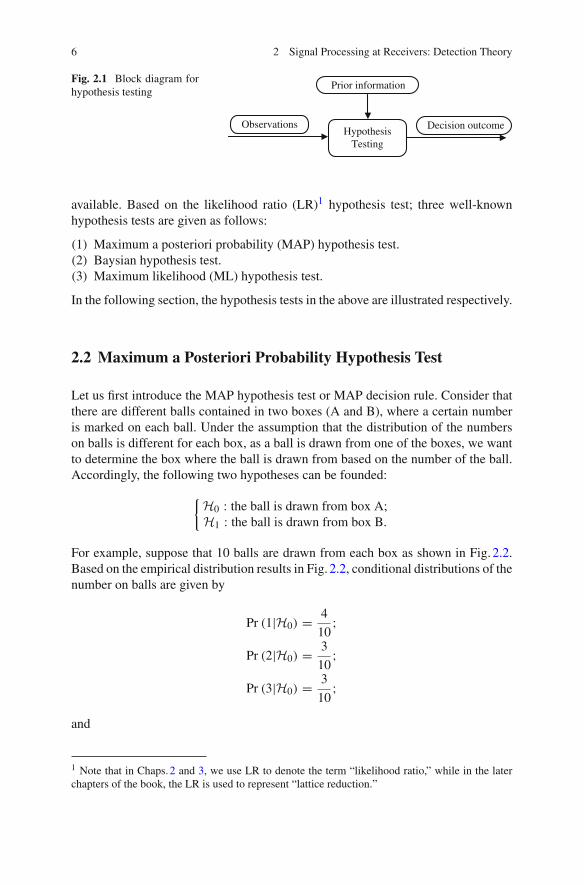
The decision process or hypothesis testing is illustrated in Fig. 2.1. In Fig. 2.1, isshown that observations and prior information are taken into account to obtain thefinal decision. However, considering the cases that no prior information is availableor prior information could be useless, the hypothesis test can also be developed withobservations only.
Under the assumption that there exist M(≥ 2) hypotheses, we can have an M-aryhypothesis testing in which we need to choose one of the M hypotheses that explainsobservations and prior information best. In order to choose a hypothesis, differentcriteria can be considered. According to these criteria, different hypothesis tests are
L. Bai et al., Low Complexity MIMO Receivers, DOI: 10.1007/978-3-319-04984-7_2, 5© Springer International Publishing Switzerland 2014
6 2 Signal Processing at Receivers: Detection Theory
Fig. 2.1 Block diagram forhypothesis testing
HypothesisTesting
Observations
Prior information
Decision outcome
available. Based on the likelihood ratio (LR)1 hypothesis test; three well-knownhypothesis tests are given as follows:
(1) Maximum a posteriori probability (MAP) hypothesis test.(2) Baysian hypothesis test.(3) Maximum likelihood (ML) hypothesis test.
In the following section, the hypothesis tests in the above are illustrated respectively.
2.2 Maximum a Posteriori Probability Hypothesis Test
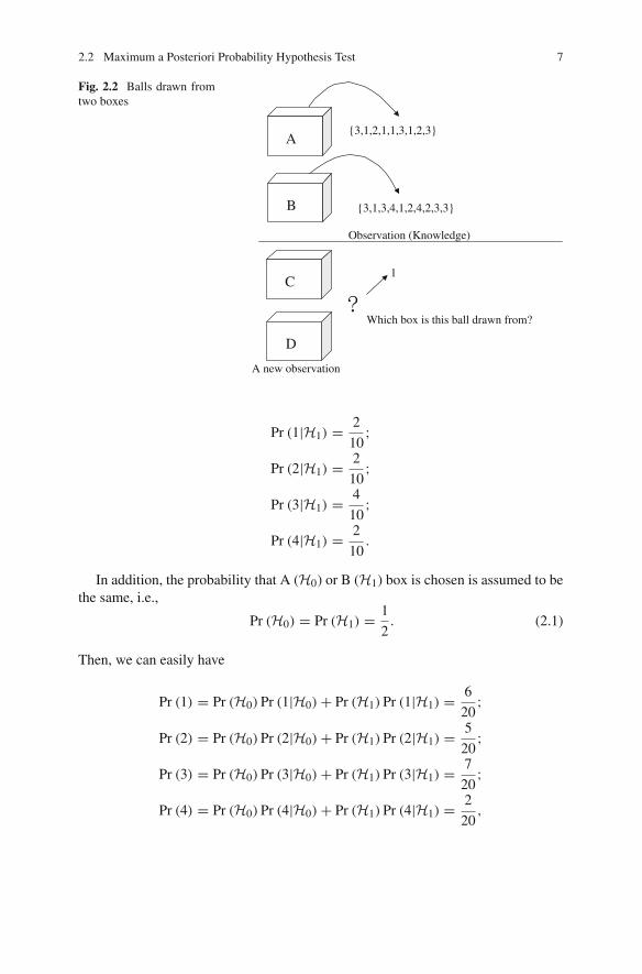
Let us first introduce the MAP hypothesis test or MAP decision rule. Consider thatthere are different balls contained in two boxes (A and B), where a certain numberis marked on each ball. Under the assumption that the distribution of the numberson balls is different for each box, as a ball is drawn from one of the boxes, we wantto determine the box where the ball is drawn from based on the number of the ball.Accordingly, the following two hypotheses can be founded:
{H0 : the ball is drawn from box A;H1 : the ball is drawn from box B.
For example, suppose that 10 balls are drawn from each box as shown in Fig. 2.2.Based on the empirical distribution results in Fig. 2.2, conditional distributions of thenumber on balls are given by
Pr (1|H0) = 4
10;
Pr (2|H0) = 3
10;
Pr (3|H0) = 3
10;
and
1 Note that in Chaps. 2 and 3, we use LR to denote the term “likelihood ratio,” while in the laterchapters of the book, the LR is used to represent “lattice reduction.”
2.2 Maximum a Posteriori Probability Hypothesis Test 7
Fig. 2.2 Balls drawn fromtwo boxes
Observation (Knowledge)
A new observation
Which box is this ball drawn from?
{3,1,2,1,1,3,1,2,3}
{3,1,3,4,1,2,4,2,3,3}
A
B
C
D
1
Pr (1|H1) = 2
10;
Pr (2|H1) = 2
10;
Pr (3|H1) = 4
10;
Pr (4|H1) = 2
10.
In addition, the probability that A (H0) or B (H1) box is chosen is assumed to bethe same, i.e.,
Pr (H0) = Pr (H1) = 1
2. (2.1)
Then, we can easily have
Pr (1) = Pr (H0) Pr (1|H0) + Pr (H1) Pr (1|H1) = 6
20;
Pr (2) = Pr (H0) Pr (2|H0) + Pr (H1) Pr (2|H1) = 5
20;
Pr (3) = Pr (H0) Pr (3|H0) + Pr (H1) Pr (3|H1) = 7
20;
Pr (4) = Pr (H0) Pr (4|H0) + Pr (H1) Pr (4|H1) = 2
20,
8 2 Signal Processing at Receivers: Detection Theory
where Pr (n) denotes the probability that the ball with number n is drawn. TakingPr(Hk) as the a priori probability (APRP) of Hk , the a posteriori probability (APP)of Hk is shown as follows:
Pr (H0|1) = 2
3;
Pr (H0|2) = 3
5;
Pr (H0|3) = 3
7;
Pr (H0|4) = 0,
and
Pr (H1|1) = 1
3;
Pr (H1|2) = 2
5;
Pr (H1|3) = 4
7;
Pr (H1|4) = 1.
Here, Pr (Hk |n) is formed as the conditional probability that the hypothesis Hk istrue under the condition that the number on the drawn ball is n. For example, if thenumber of the ball is n = 1, since Pr (H0|1) = 2
3 is greater than Pr (H1|1) = 13 , we
can decide that the ball is drawn from box A, where the hypothesis H0 is accepted.The corresponding decision rule is named as the MAP hypothesis testing, since wechoose the hypothesis that maximizes the APP.
Generally, in the binary hypothesis testing, H0 and H1 are referred to as the nullhypothesis and the alternative hypothesis, respectively. Under the assumption thatthe APRPs Pr(H0) and Pr(H1) are known and the conditional probability, Pr(Y |Hk),is given, where Y denotes the random variable for an observation, the MAP decisionrule for binary hypothesis testing is given by
{H0 : Pr (H0|Y = y) > Pr (H1|Y = y) ;H1 : Pr (H0|Y = y) < Pr (H1|Y = y) ,
(2.2)
where y denotes the realization of Y . Note that H0 is chosen if Pr (H0|Y = y) >
Pr (H1|Y = y) and vice versa. Here, we do not consider the case of Pr (H0|Y = y) =Pr (H1|Y = y) in (2.2), where a decision can be made arbitrarily. Thus, the decisionoutcome in (2.3) can be considered as a function of y. Using Bayes rule, we can alsoshow that ⎧⎪⎪⎨
⎪⎪⎩H0 : Pr (Y = y|H0)
Pr (Y = y|H1)>
Pr (H1)
Pr (H0);
H1 : Pr (Y = y|H0)
Pr (Y = y|H1)<
Pr (H1)
Pr (H0).
(2.3)
2.2 Maximum a Posteriori Probability Hypothesis Test 9
ys
f (y ) = (0,σ2 ) f ( y ) = (s,σ2 )0 1
Fig. 2.3 The pdf of the hypothesis pair
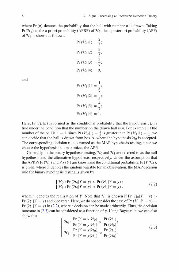
Notice that as Y is a continuous random variable, Pr (Y = y|Hk) is replaced byf (Y = y|Hk), where f (Y = y|Hk) represents the conditional probability densityfunction (pdf) of Y given Hk .
Example 2.1. Define by N (μ,σ2
)the pdf of a Gaussian random variable (i.e., x)
with mean μ and variance σ2, where
N(μ,σ2
)=
exp(− (x−μ)2
2σ2
)√
2πσ2. (2.4)
Let the noise n be a Gaussian random variable with mean zero and variance σ, whiles be a positive constant. Consider the case that a constant signal, s, is transmitted,while a received signal, y, may be corrupted by the noise, n, as shown in Fig. 2.3.Then, we can have the following hypothesis pair to decide whether or not s is presentwhen y is corrupted by n: {H0 : y = n;
H1 : y = s + n.(2.5)
Then, as shown in Fig. 2.3, we have
{f (y|H0) = N (
0,σ2) ;
f (y|H1) = N (s,σ2
),
(2.6)
andf (Y = y|H0)
f (Y = y|H1)= exp
(− s(2y − s)
2σ2
), (2.7)
when s > 0. Letting
ρ = Pr(H0)
Pr(H1),
the MAP decision rule is simplified as follows:
10 2 Signal Processing at Receivers: Detection Theory
Table 2.1 MAP decision rule Accept H0 H1
H0 is true Correct Type I (false alarm)H1 is true Type II (miss) Correct (detection)
Table 2.2 The probabilitiesof type I and II errors
Error type Case Error probability
Type I Accept H1 when H0 is true PA
Type II Accept H0 when H1 is true PB
⎧⎪⎪⎨⎪⎪⎩H0 : y <
s
2+ σ2 ln ρ
s;
H1 : y >s
2+ σ2 ln ρ
s.
(2.8)
Since the decision rule is a function of y, we can express the decision rule asfollows: {
r(y) = 0 : y ∈ A0;r(y) = 1 : y ∈ A1,
(2.9)
where A0 and A1 represent the decision regions of H0 and H1, respectively. There-fore, for the MAP decision rule in (2.8), the corresponding decision regions aregiven by ⎧⎪⎪⎨
⎪⎪⎩A0 =
{y | y <
s
2− σ2 ln ρ
s
};
A1 ={
y | y >s
2− σ2 ln ρ
s
},
(2.10)
where A0 and A1 are regarded as the acceptance region and the rejection/criticalregion, respectively, in the binary hypothesis testing.
Table 2.1 shows four possible cases of decision, where type I and II errors areusually carried out to analyze the performance. Note that since the null hypothesis,H0, normally represents the case that no signal is present, while the other hypothesis,H1, represents the case that a signal is present, the probabilities of type I and II errorsare regarded as the false alarm and miss probabilities, respectively. The two types ofdecision errors are summarized in Table 2.2. Using the decision rule r(y), PA andPB are given by
PA = Pr (Y ∈ A1|H0) (2.11)
=∫
r(y) f (y|H0)dy (2.12)
= E [r(Y )|H0] (2.13)
and
2.2 Maximum a Posteriori Probability Hypothesis Test 11
PB = Pr (Y ∈ A0|H1) (2.14)
=∫
(1 − r(y)) f (y|H1)dy (2.15)
= E [(1 − r(Y ))|H1] , (2.16)
respectively. Then, the probability of detection becomes
PD = 1 − PB (2.17)
= E [r(Y )|H1] . (2.18)
2.3 Baysian Hypothesis Test
In order to minimize the cost associated with the decision, the Baysian decision ruleis carried out. Denote by Dk the decision that acceptsHk , while by Gik the associatedcost of Di when the hypothesis Hk is true. Assuming the cost of erroneous decisionto be higher than that of correct decision, we have G10 > G00 and G01 > G11. Theaverage cost E [Gik] is given by
G = E [Gik] (2.19)
=∑
i
∑k
Gik Pr (Di ,Hk) (2.20)
=∑
i
∑k
Gik P (Di |Hk) Pr (Hk) . (2.21)
Let Ac0 denote the complementary set of the decision region, A0, and assume that
A1 = Ac0 for convenience. Since
Pr (D1|Hk) = 1 − (D0|Hk) , (2.22)
the average cost in (2.21) is rewritten as
G = G10 Pr(H0) + G11 Pr(H1) +∫A0
g1(y) − g0(y)dy, (2.23)
where {g0(y) = Pr(H0)(G10 − G00) f (y|H0);g1(y) = Pr(H1)(G01 − G11) f (y|H1).
(2.24)
Then, it is possible to minimize the average cost G by properly defining the accep-tance regions, while the problem is formulated as
12 2 Signal Processing at Receivers: Detection Theory
minA0,A1
G. (2.25)
Since (2.23) follows
G = Constant +∫A0
g1(y) − g0(y)dy, (2.26)
we can show that
minA0
G ⇔ minA0
{∫A0
g1(y) − g0(y)dy
}, (2.27)
while the optimal regions that minimize the cost are given by
{A0 = {y|g1(y) ≤ g0(y)} ;A1 = {y|g1(y) > g0(y)} .
(2.28)
Hence, we can conclude the Baysian decision rule that minimizes the cost as follows:
{H0 : g0(y) > g1(y);H1 : g0(y) < g1(y),
(2.29)
or ⎧⎪⎪⎨⎪⎪⎩H0 : f (y|H0)
f (y|H1)>
Pr(H0)
Pr(H1)
G01 − G11
G10 − G00;
H1 : f (y|H0)
f (y|H1)<
Pr(H0)
Pr(H1)
G01 − G11
G10 − G00,
(2.30)
where (G10 − G00) and (C01 − C11) are positive. More importantly, for binaryhypothesis testing, we can find out that the ratio of the cost differences, G01−G11
G10−G00,
is able to characterize the Baysian decision rule rather than the values of individualcosts, Gik’s. Specifically, as G01−G11
G10−G00= 1, the Baysian hypothesis test becomes the
MAP hypothesis test.
2.4 Maximum Likelihood Hypothesis Test
The MAP decision rule can be employed under the condition that the APRP isavailable. Considering the case that the APRP is not available, another decision rulebased on likelihood functions can be developed. For a given value of observation, y,the likelihood function is defined by
{f0(y) = f (y|H0);f1(y) = f (y|H1).
(2.31)
2.4 Maximum Likelihood Hypothesis Test 13
Notice that the likelihood function is not a function of y since y is given, but afunction of the hypothesis. With respect to the ML function, the ML decision rule isto choose the hypothesis as follows:
{H0 : f0(y) > f1(y);H1 : f0(y) < f1(y),
⇔
⎧⎪⎪⎨⎪⎪⎩H0 : f0(y)
f1(y)> 1;
H1 : f0(y)
f1(y)< 1,
(2.32)
where the ratio, f0(y)f1(y)
, is regarded as the LR. For convenience, given by
LLR(y) = logf0(y)
f1(y)(2.33)
the e-based log-likelihood ratio (LLR), the ML decision rule can be rewritten as
{H0 : LLR(y) > 0;H1 : LLR(y) < 0.
(2.34)
Note that the ML decision rule can be considered as a special case of the MAPdecision rule when the APRPs are the same, i.e., Pr(H0) = Pr(H1). In this case, theMAP decision rule is reduced to the ML decision rule.
2.5 Likelihood Ratio-Based Hypothesis Test
Let the LR-based decision rule be
⎧⎪⎪⎨⎪⎪⎩H0 : f0(y)
f1(y)> ρ;
H1 : f0(y)
f1(y)< ρ,
(2.35)
where ρ denotes a predetermined threshold. Consider the following hypothesis pairof received signals: {H0 : y = μ0 + n;
H1 : y = μ1 + n,(2.36)
where μ1 > μ0 and n ∼ N (0,σ2). Then, it follows that
{f0(y) = N (μ0,σ
2);f1(y) = N (μ1,σ
2),(2.37)
14 2 Signal Processing at Receivers: Detection Theory
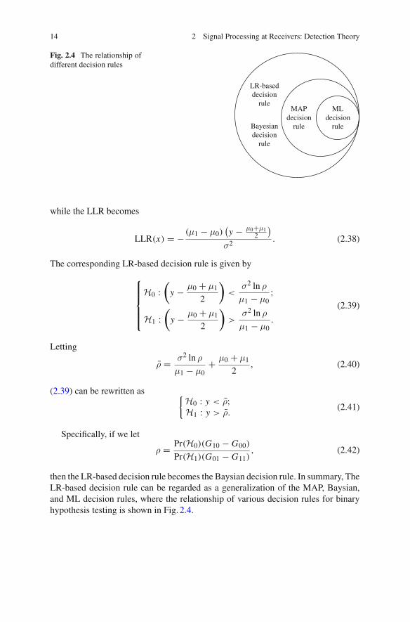
Fig. 2.4 The relationship ofdifferent decision rules
MLdecision
rule
MAPdecision
rule
LR-baseddecision
rule
Bayesiandecision
rule
while the LLR becomes
LLR(x) = − (μ1 − μ0)(y − μ0+μ1
2
)σ2 . (2.38)
The corresponding LR-based decision rule is given by
⎧⎪⎪⎪⎨⎪⎪⎪⎩H0 :
(y − μ0 + μ1
2
)<
σ2 ln ρ
μ1 − μ0;
H1 :(
y − μ0 + μ1
2
)>
σ2 ln ρ
μ1 − μ0.
(2.39)
Letting
ρ = σ2 ln ρ
μ1 − μ0+ μ0 + μ1
2, (2.40)
(2.39) can be rewritten as {H0 : y < ρ;H1 : y > ρ.
(2.41)
Specifically, if we let
ρ = Pr(H0)(G10 − G00)
Pr(H1)(G01 − G11), (2.42)
then the LR-based decision rule becomes the Baysian decision rule. In summary, TheLR-based decision rule can be regarded as a generalization of the MAP, Baysian,and ML decision rules, where the relationship of various decision rules for binaryhypothesis testing is shown in Fig. 2.4.
2.6 Neyman–Pearson Lemma 15
2.6 Neyman–Pearson Lemma
It is possible to define the Correct (detection) and type I error (false alarm) probabili-ties for each decision rule. On the contrary, for a given target detection probability orerror probability, we may be able to derive an optimal decision rule. Let us considerthe following optimization problem:
maxd
PD(d) subject to PA(d) ≤ σ, (2.43)
where d and σ represent a decision rule and the maximum false alarm probabilities,respectively. In order to find the decision rule, d, with the maximum false alarmprobability constraint, the Neyman–Pearson Lemma is presented as follows.
Lemma 2.1. Let the decision rule of d ′(s) be
d ′(s) =
⎧⎪⎪⎨⎪⎪⎩
1, if f1(s) > η f0(s);γ(s) =
{1, with probability p;0, with probability 1 − p,
if f1(s) = η f0(s);0, if f1(s) < η f0(s),
(2.44)
where η > 0 and p is decided such that PA = σ. The decision rule in (2.44) isnamed as the Neyman–Pearson (NP) rule and becomes the solution of the problemin (2.43).
Proof. Under the condition of PA ≤ σ, we can assume that the decision rule becomesd. In order to show the optimality of the problem in (2.43), we need to verify thatfor any d, we have PD(t ′) ≥ PD(t). Denote by S the observation set, where s ∈ S.Using the definition of d ′, for any s ∈ S, it shows that
(d ′(s) − d(s)
)( f1(s) − η f0(s)) ≥ 0. (2.45)
Then, it is derived that
∫s∈S
(d ′(s) − d(s)
)( f1(s) − η f0(s)) ds ≥ 0 (2.46)
and∫
s∈Sd ′(s) f1(s)ds −
∫s∈S
d(s) f1(s)ds ≥ η
(∫s∈S
d ′(s) f0(s)ds −∫
s∈Sd(s) f0(s)ds
),
(2.47)which can further show that
PD(d ′) − PD(d) ≥ η(
PA(d ′) − PA(d))
≥ 0. (2.48)
16 2 Signal Processing at Receivers: Detection Theory
Since (2.48) shows that PD(d ′) ≥ PD(d), the proof is completed. �
From (2.43), we can show that the NP decision rule is the same as the LR-baseddecision rule with the threshold ρ = 1
η except the randomized rule, i.e., f1(s) =η f0(s).
Example 2.2. Let us consider the following hypothesis pair:
{H0 : y = n;H1 : y = s + n,
(2.49)
where s > 0 and n ∼ N (0,σ2). Using (2.41), the type I error probability is shown as
� =∫ ∞
−∞d(y) f0(y)dy
=∫ ∞
ρf0(y)dy
=∫ ∞
ρ
1√2πσ2
exp
(− y2
2σ2
)dy
= Q(
ρ
σ
),
where Q(x) denotes the Q-function and is defined by
Q(x) =∫ ∞
x
1√2π
e−t2/2dt. (2.50)
Note that the function Q(x), x ≥ 0, is the tail of the normalized Gaussian pdf (i.e.,N (0, 1)) from x to ∞. Then, it follows that
� = Q(
ρ
σ
)(2.51)
orρ = σQ−1(�). (2.52)
Thus, the detection probability becomes
PD =∫ ∞
ρf1(y)dy
=∫ ∞
ρ
1√2πN 2
0
exp
(− (y − s)2
2N 20
)dy
2.6 Neyman–Pearson Lemma 17
0 0.1 0.2 0.3 0.4 0.5 0.6 0.7 0.8 0.9 10
0.1
0.2
0.3
0.4
0.5
0.6
0.7
0.8
0.9
1
Δ
PD
s = 2s = 1s = 0.5
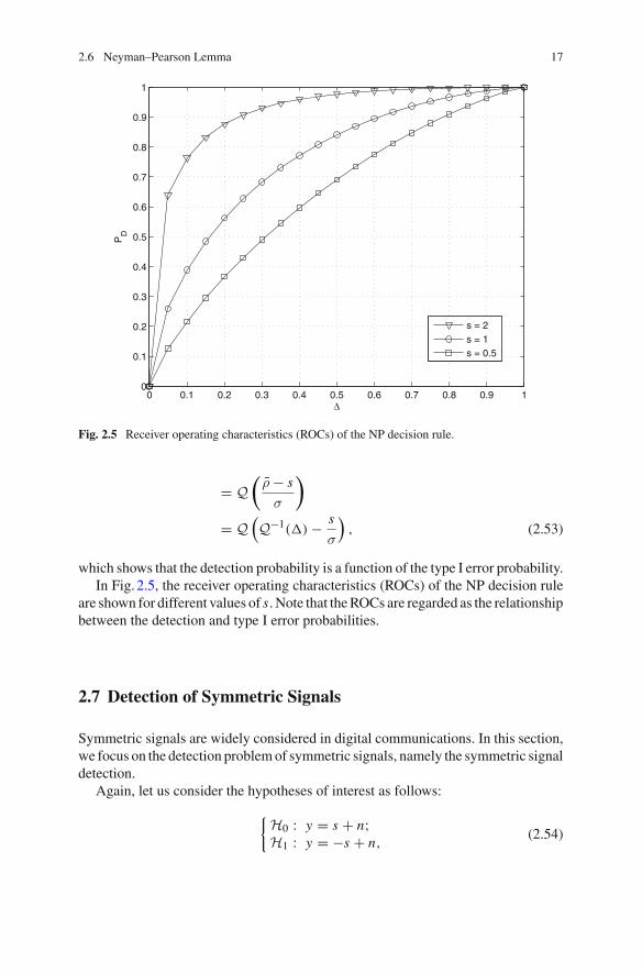
Fig. 2.5 Receiver operating characteristics (ROCs) of the NP decision rule.
= Q(
ρ − s
σ
)
= Q(Q−1(�) − s
σ
), (2.53)
which shows that the detection probability is a function of the type I error probability.In Fig. 2.5, the receiver operating characteristics (ROCs) of the NP decision rule
are shown for different values of s. Note that the ROCs are regarded as the relationshipbetween the detection and type I error probabilities.
2.7 Detection of Symmetric Signals
Symmetric signals are widely considered in digital communications. In this section,we focus on the detection problem of symmetric signals, namely the symmetric signaldetection.
Again, let us consider the hypotheses of interest as follows:
{H0 : y = s + n;H1 : y = −s + n,
(2.54)
18 2 Signal Processing at Receivers: Detection Theory
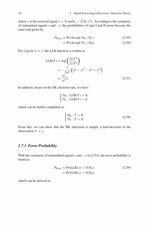
where y is the received signal, s > 0, and n ∼ N (0,σ2). According to the symmetryof transmitted signals s and −s, the probabilities of type I and II errors become thesame and given by
PError = Pr(Accept H0 | H1) (2.55)
= Pr(Accept H1 | H0). (2.56)
For a given Y = y, the LLR function is written as
LLR(Y ) = log
(f0(Y )
f1(Y )
)
= − 1
2σ2
((Y − s)2 − (Y + s)2
)
= 2s
σ2 Y. (2.57)
In addition, based on the ML decision rule, we have
{H0 : LLR(Y ) > 0;H1 : LLR(Y ) < 0,
which can be further simplified as
{H0 : Y > 0;H1 : Y < 0.
(2.58)
From this, we can show that the ML detection is simply a hard-decision of theobservation Y = y.
2.7.1 Error Probability
With the symmetry of transmitted signals s and −s in (2.54), the error probability isfound as
PError = Pr(LLR(y) > 0|H1) (2.59)
= Pr(LLR(y) < 0|H0),
which can be derived as
2.7 Detection of Symmetric Signals 19
PError = Pr(LLR(y) > 0|H1)
= Pr(y > 0|H1)
=∫ ∞
0
1√2πσ
exp
(− 1
2σ2 (Y + s)2)
dY (2.60)
and
PError =∫ ∞
sσ
1√2π
exp
(−Y 2
2
)dY
= Q( s
σ
). (2.61)
Letting the signal-to-noise ratio (SNR) be SNR = s2
σ2 , then we can have PError =Q(
√SNR). Note that the error probability decreases with the SNR, since Q is a
decreasing function.
2.7.2 Bound Analysis
In order to show the characteristics of the error probability, let us derive the boundson the error probability. Define the error function as
erf(y) = 2√π
∫ y
0exp
(−y2
)dy (2.62)
and the complementary error function as
erfc(y) = 1 − erfc(y) (2.63)
= 2√π
∫ ∞
yexp
(−t2
)dt, for y > 0,
where the relationship between the Q-function and the complementary error functionis given by
erfc(y) = 2Q(√
2y)
;
Q(y) = 1
2erfc
(y√2
). (2.64)
Then, for a given Y = y, we can show that the complementary error function hasthe following bounds:
20 2 Signal Processing at Receivers: Detection Theory
(1 − 1
2Y 2
)exp
(−Y 2)
√πY
< erfc(Y ) <exp
(−Y 2)
√πY
, (2.65)
where the lower bound is valid if Y > 1/√
2. Accordingly, the Q-function Q(Y ) isbounded as follows:
(1 − 1
Y 2
)exp
(−Y 2/2)
√2πY
< Q(Y ) <exp
(−Y 2/2)
√2πY
, (2.66)
where the lower bound is valid if x > 1. Thus, the upper bound of error probabilityis given by
PError = Q(√
SNR) <exp (−SNR/2)√
2π√
SNR. (2.67)
In order to obtain an upper bound on the probability of an event that happens rarely,the Chernoff bound is widely considered, which can be used for any backgroundnoise.
Let p(y) denote the step function, where p(y) = 1, if y ≥ 0, and p(y) = 0, ify < 0. Using the step function, the probability for the event that Y ≥ y, which canbe also regarded as the tail probability, is given by
Pr(Y ≥ y) =∫ ∞
yfY (ρ)dρ
=∫ ∞
−∞p(ρ − y) fY (ρ)dρ
= E[p(Y − y)], (2.68)
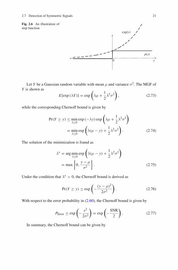
where fY (ρ) represents the pdf of Y . From Fig. 2.6, we can show that
p(y) ≤ exp(y). (2.69)
Thus, we can havePr(Y ≥ y) ≤ E[exp(Y − y)] (2.70)
orPr(Y ≥ y) ≤ E
[exp (λ(Y − y))
](2.71)
for λ ≥ 0. By minimizing the right-hand side with respect to λ in (2.71), the tightestupper bound can be obtained which is regarded as the Chernoff bound and given by
Pr(Y ≥ y) ≤ minλ≥0
exp (−λy) E[exp (λY )
]. (2.72)
In (2.72), E[exp (λY )
]is called the moment generating function (MGF).
2.7 Detection of Symmetric Signals 21
Fig. 2.6 An illustration ofstep function
exp(y)
p(y)
y0
Let Y be a Gaussian random variable with mean μ and variance σ2. The MGF ofY is shown as
E[exp (λY )] = exp
(λμ + 1
2λ2σ2
), (2.73)
while the corresponding Chernoff bound is given by
Pr(Y ≥ y) ≤ minλ≥0
exp (−λy) exp
(λμ + 1
2λ2σ2
)
= minλ≥0
exp
(λ(μ − y) + 1
2λ2σ2
). (2.74)
The solution of the minimization is found as
λ∗ = arg minλ≥0
exp
(λ(μ − y) + 1
2λ2σ2
)
= max
{0,
y − μ
σ2
}. (2.75)
Under the condition that λ∗ > 0, the Chernoff bound is derived as
Pr(Y ≥ y) ≤ exp
(− (y − μ)2
2σ2
). (2.76)
With respect to the error probability in (2.60), the Chernoff bound is given by
PError ≤ exp
(− s2
2σ2
)= exp
(−SNR
2
). (2.77)
In summary, the Chernoff bound can be given by
22 2 Signal Processing at Receivers: Detection Theory
Q(y) ≤ exp
(− y2
2
), (2.78)
which is actually a special case of the Chernoff bound in (2.72).
2.8 Binary Signal Detection
In general, signals are transmitted by waveforms rather than discrete signals overwireless channels. Using binary signaling, for 0 ≤ t < T , the received signal can bewritten as
Y (t) = S(t) + N (t), 0 ≤ t < T, (2.79)
where T and N (t) denote the signal duration and a white Gaussian random process,respectively. Note that we have E[N (t)] = 0 and E[N (t)N (ρ)] = N0
2 δ(t − ρ),where δ(t) represents the Dirac delta function. The channel in (2.79) is called theadditive white Gaussian noise (AWGN) channel, while S(t) is a binary waveformthat is given by
{under hypothesis H0 : S(t) = s0(t);under hypothesis H0 : S(t) = s1(t).
(2.80)
Note that the transmission rate is 1T bits per second for the signaling in (2.79).
Let a heuristic approach be carried out to deal with waveform signal detectionproblem. At the receiver, the decision is made with Y (t), 0 ≤ t < T . Denote by y(t)a realization or observation of Y (t), where L samples are taken from y(t). Lettings(t) and n(t) be a realization of S(t) and N (t), respectively, we can have
yl =∫ lT
L
(l−1)TL
y(t)dt,
sm,l =∫ lT
L
(l−1)TL
sm(t)dt,
nl =∫ lT
L
(l−1)TL
n(t)dt, (2.81)
where{H0 : yl = s0,l + nl;H1 : yl = s1,l + nl .
(2.82)
In addition, since N (t) is a white process, the nl ’s are independent, while the meanof nl is zero and the variance can be derived as
2.8 Binary Signal Detection 23
σ2 = E[n2l ]
= E
⎡⎣
(∫ lTL
(l−1)TL
N (t)dt
)2⎤⎦
=∫ lT
L
(l−1)TL
∫ lTL
(l−1)TL
E[N (t)N (ρ)]dtdρ
=∫ lT
L
(l−1)TL
∫ lTL
(l−1)TL
N0
2δ(t − ρ)dtdρ
= N0T
2L. (2.83)
Letting y = [y1 y2 · · · yL ]T, the LLR becomes
LLR(y) =∏L
l=1 f (yl |H0)∏Ll=1 f (yl |H1)
(2.84)
= logf0(y)
f1(y),
which follows that
LLR(y) =L∑
l=1
logf0(yl)
f1(yl)
=L∑
l=1
log
[exp
(− 1
N0
((yl − s0,l)
2 − (yl − s1,l)2))]
= 1
N0
L∑l=1
((yl − s1,l)
2 − (yl − s0,l)2)
= 1
N0
(L∑
l=1
2yl(s0,l − s1,l) +L∑
l=1
(s21,l − s2
0,l)
). (2.85)
In addition, letting sm = [sm,1 sm,2 . . . sm,L ]T, (2.85) can be rewritten as
LLR(y) = 1
N0
(2yT(s0 − s1) − (sT
0 s0 − sT1 s1)
). (2.86)
From the LLR in (2.86), the MAP decision rule is given by
24 2 Signal Processing at Receivers: Detection Theory
⎧⎪⎪⎪⎨⎪⎪⎪⎩
H0 : yT(s0 − s1) > σ2 log
(Pr(H1)
Pr(H2)
)+ 1
2(sT
0 s0 − sT1 s1);
H1 : yT(s0 − s1) < σ2 log
(Pr(H1)
Pr(H2)
)+ 1
2(sT
0 s0 − sT1 s1).
(2.87)
For the LR-based decision rule, we can replace Pr(H0)Pr(H1)
by the threshold ρ, which is
⎧⎪⎪⎨⎪⎪⎩H0 : yT(s0 − s1) > σ2 log ρ + 1
2(sT
0 s0 − sT1 s1);
H1 : yT(s0 − s1) < σ2 log ρ + 1
2(sT
0 s0 − sT1 s1).
(2.88)
As the number of samples during T seconds is small, there could be signal infor-mation loss due to sampling operation using the approach in (2.81). To avoid anysignal information loss, suppose that L is sufficiently large to approximate as
yTsi ≈ 1
T
∫ T
0y(t)sm(t)dt. (2.89)
Accordingly, the LR-based decision rule can be written as
⎧⎪⎨⎪⎩H0 : ∫ T
0 y(t)(s0(t) − s1(t))dt > σ2 log ρ + 1
2
∫ T0
(s2
0 (t) − s21 (t)
)dt;
H1 : ∫ T0 y(t)(s0(t) − s1(t))dt < σ2 log ρ + 1
2
∫ T0
(s2
0 (t) − s21 (t)
)dt,
(2.90)
or ⎧⎨⎩H0 : ∫ T
0 y(t)(s0(t) − s1(t))dt > WT ;H1 : ∫ T
0 y(t)(s0(t) − s1(t))dt < WT ,(2.91)
if we let
WT = σ2 log ρ + 1
2
∫ T
0
(s2
0 (t) − s21 (t)
)dt. (2.92)
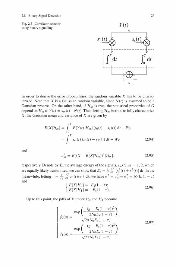
Note that the decision rule is named as the correlator detector, which can be imple-mented as in Fig. 2.7.
Let us then analyze its performance. For the ML decision rule, we can have ρ = 1in the LR-based decision rule, which leads to WT = 1
2
∫ T0
(s2
0 (t) − s21 (t)
)dt. Letting
X = ∫ T0 y(t) (s0(t) − s1(t)) dt − WT , we can show that
{Pr(D0|H1) = Pr(X > 0|H1);Pr(D1|H0) = Pr(X < 0|H0).
(2.93)
2.8 Binary Signal Detection 25
Fig. 2.7 Correlator detectorusing binary signalling
In order to derive the error probabilities, the random variable X has to be charac-terized. Note that X is a Gaussian random variable, since N (t) is assumed to be aGaussian process. On the other hand, if Hm is true, the statistical properties of Gdepend onHm as Y (t) = sm(t)+N (t). Then, lettingHm be true, to fully characterizeX , the Gaussian mean and variance of X are given by
E[X |Hm] =∫ T
0E[Y (t)|Hm] (s0(t) − s1(t)) dt − WT
=∫ T
0sm(t) (s0(t) − s1(t)) dt − WT (2.94)
andσ2
m = E[(X − E[X |Hm])2|Hm], (2.95)
respectively. Denote by Es the average energy of the signals, sm(t), m = 1, 2, whichare equally likely transmitted, we can show that Es = 1
2
∫ T0
(s2
0 (t) + s21 (t)
)dt . In the
meanwhile, letting τ = 1Es
∫ T0 s0(t)s1(t)dt , we have σ2 = σ2
0 = σ21 = N0 Es(1 − τ )
and {E[X |H0] = Es(1 − τ );E[X |H1] = −Es(1 − τ ).
(2.96)
Up to this point, the pdfs of X under H0 and H1 become
⎧⎪⎪⎪⎪⎪⎪⎪⎨⎪⎪⎪⎪⎪⎪⎪⎩
f0(g) =exp
(− (g − Es(1 − τ ))2
2N0 Es(1 − τ )
)√
2πN0 Es(1 − τ );
f1(g) =exp
(− (g + Es(1 − τ ))2
2N0 Es(1 − τ )
)√
2πN0 Es(1 − τ ).
(2.97)
26 2 Signal Processing at Receivers: Detection Theory
By following the same approach in Sect. 2.7.1, the error probability can be derived as
PError = Q(√
Es(1 − τ )
N0
). (2.98)
For a fixed signal energy, Es, since the error probability can be minimized whenτ = −1, the corresponding minimum error probability can be written as
PError = Q(√
2Es
N0
). (2.99)
Note that the resulting signals that minimize the error probability are regarded asantipodal signals, which can be easily shown as s0(t) = −s1(t). In addition, for anorthogonal signal set where ρ = 0, we have the corresponding error probability to be
PError = Q(√
Es
N0
). (2.100)
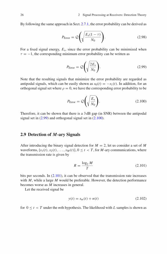
Therefore, it can be shown that there is a 3 dB gap (in SNR) between the antipodalsignal set in (2.99) and orthogonal signal set in (2.100).
2.9 Detection of M-ary Signals
After introducing the binary signal detection for M = 2, let us consider a set of Mwaveforms, {s1(t), s2(t), . . . , sM (t)}, 0 ≤ t < T , for M-ary communications, wherethe transmission rate is given by
R = log2 M
T(2.101)
bits per seconds. In (2.101), it can be observed that the transmission rate increaseswith M , while a large M would be preferable. However, the detection performancebecomes worse as M increases in general.
Let the received signal be
y(t) = sm(t) + n(t) (2.102)
for 0 ≤ t < T under the mth hypothesis. The likelihood with L samples is shown as
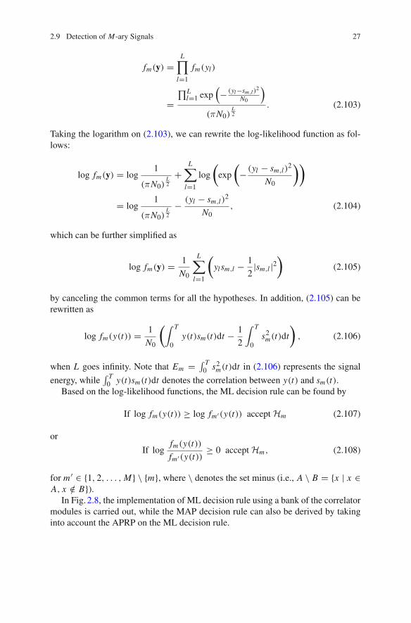
2.9 Detection of M-ary Signals 27
fm(y) =L∏
l=1
fm(yl)
=∏L
l=1 exp(− (yl−sm,l )
2
N0
)
(πN0)L2
. (2.103)
Taking the logarithm on (2.103), we can rewrite the log-likelihood function as fol-lows:
log fm(y) = log1
(πN0)L2
+L∑
l=1
log
(exp
(− (yl − sm,l)
2
N0
))
= log1
(πN0)L2
− (yl − sm,l)2
N0, (2.104)
which can be further simplified as
log fm(y) = 1
N0
L∑l=1
(ylsm,l − 1
2|sm,l |2
)(2.105)
by canceling the common terms for all the hypotheses. In addition, (2.105) can berewritten as
log fm(y(t)) = 1
N0
(∫ T
0y(t)sm(t)dt − 1
2
∫ T
0s2
m(t)dt
), (2.106)
when L goes infinity. Note that Em = ∫ T0 s2
m(t)dt in (2.106) represents the signal
energy, while∫ T
0 y(t)sm(t)dt denotes the correlation between y(t) and sm(t).Based on the log-likelihood functions, the ML decision rule can be found by
If log fm(y(t)) ≥ log fm′(y(t)) accept Hm (2.107)
or
If logfm(y(t))
fm′(y(t))≥ 0 accept Hm, (2.108)
for m′ ∈ {1, 2, . . . , M} \ {m}, where \ denotes the set minus (i.e., A \ B = {x | x ∈A, x /∈ B}).
In Fig. 2.8, the implementation of ML decision rule using a bank of the correlatormodules is carried out, while the MAP decision rule can also be derived by takinginto account the APRP on the ML decision rule.
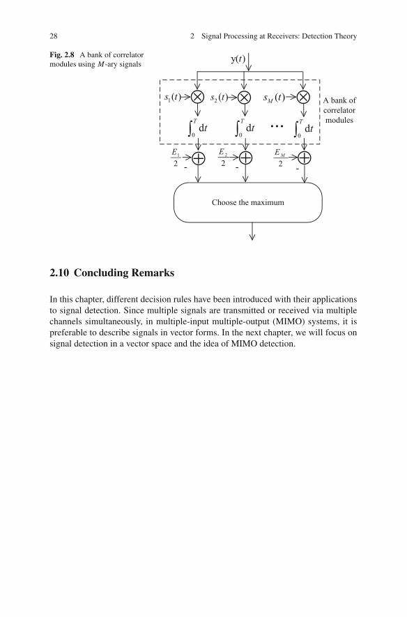
28 2 Signal Processing at Receivers: Detection Theory
Fig. 2.8 A bank of correlatormodules using M-ary signals
2.10 Concluding Remarks
In this chapter, different decision rules have been introduced with their applicationsto signal detection. Since multiple signals are transmitted or received via multiplechannels simultaneously, in multiple-input multiple-output (MIMO) systems, it ispreferable to describe signals in vector forms. In the next chapter, we will focus onsignal detection in a vector space and the idea of MIMO detection.

http://www.springer.com/978-3-319-04983-0