Side Effects of Immunities: the African Slave Trade∗

Elena EspositoEuropean University Institute†

Working Paper

October 29, 2015

Abstract

Why was slavery concentrated in the South of the United States? And why were certainAfrican populations extensively raided to be enslaved in those regions? The novel empiri-cal evidence presented in this paper reveals that (i) malaria was a major determinant forthe diffusion of African slavery in the southern United States and (ii) malaria-resistancemade sub-Saharan Africans especially attractive for employment in these regions. I firstdocument that African slavery was more widespread in those US counties subject to highermalaria exposure. Moreover, I show that the introduction of a particularly virulent, andpreviously absent, species of malaria into the United States caused a large and rapid in-crease in the prevalence of African slave labor. Finally, by looking at the historical pricesof African slaves in the Louisiana slave market, I find that more malaria-resistant slaves,i.e. those born in the most malaria-ridden regions of Africa, commanded higher prices.

Keywords: Slavery, Malaria, African Slave Trade, Colonial Institutions.

JEL Classification: I12, N31, N37, N57, J15, J47.

∗I am indebted to Matteo Cervellati for his inspiring supervision of my work. Moreover, I wish to thankOded Galor for kindly hosting me at Brown University, and Juan Dolado and Andrea Ichino for their mentor-ship at the European University Institute. Finally, comments and suggestions from Scott Abramson, FabrizioBernardi, Maristella Botticini, Graziella Bertocchi, Emilio Depetris Chauvin, Giorgio Chiovelli, Daniele Fabbri,James Fenske, Martin Fiszbein, Andrew Foster, Moshe Hazan, Eliana La Ferrara, Giorgio Gulino, John R.Logan, Ricardo Estrada Martinez, Stelios Michalopoulos, Omer Moav, Luca Pensieroso, Giovanni Prarolo,Louis Putterman, Dominic Rohner, Tim Squires, Paolo Vanin, Hans-Joachim Voth, David Weil and the otherparticipants at the Unviersity of Bologna Wednesday seminar, Brown University Macro Lunch Seminar and S4Graduate Fellow Lecture and Reception, Income Inequality Thematic Group were precious inputs for my work.†Contact details: European University Institute, Max Weber Programme, Via dei Roccettini 9, 1-50014 San

Domenico di Fiesole. E-mail: elena.esposito@eui.eu.

1

1 Introduction

There is growing evidence that the practice of slavery compromised the long-term economic

prosperity of both the enslavers and the enslaved. On the one hand, new empirical evidence

documents that slavery represents a burden for societies that historically relied on it as a source

of labor, as it has engendered long-term poverty, lower contemporary public goods provision and

higher inequality (Engerman and Sokoloff, 1997; Nunn, 2008; Dell, 2010).1 On the other hand,

slavery also appears to have stunted the long-term growth prospects of populations subject to

slave raids and enslavement - as in the case of African countries - by engendering social distrust

and fostering ethnic stratification (Nunn and Wantchekon, 2011; Whatley and Gillezeau, 2011).2

These findings have sparked significant interest in exploring what contributed to the historical

distribution of slavery, and in examining the factors that influenced and oriented the African

Slave Trade.

This paper is the first to document the role played by diseases, and notably malaria, in

determining why slavery spread in certain areas of the United States and not in others, and why

Africans - and Africans from certain regions in particular - were transported to and enslaved in

the New World so numerously. I argue that wherever in the United States malaria took root and

flourished, labor became scarcer and more expensive, slavery more economically attractive, and

malaria-resistant labor in high demand. In such areas, the malaria-resistance of Sub-Saharan

Africans increased the profitability of African slave labor, and primarily that of African slaves

from more malaria-ridden areas. Indeed, the empirical evidence I present reveals that African

slavery was largely concentrated in the more malaria-infested areas of the United States and

that it jumped after the introduction of a virulent malaria species. Moreover, by looking at

the historical prices of African slaves in the United States, I show that slaves born in regions

of Africa with higher prevalence of malaria commanded higher prices.

The hypothesis builds on two facts. First, malaria was absent from North America be-

fore European settlement. Importantly, once Europeans settled, malaria (a disease requiring

specific bio-climatic conditions for transmission) did not spread all over North America but

1See also Acemoglu, Garcıa-Jimeno, and Robinson (2012), Bertocchi and Dimico (2014) and Bobonis andMorrow (2014).

2See also Nunn (2007) and Nunn and Puga (2012).

2

became endemic only in regions which were warm and humid enough. The introduction of

the disease radically modified the epidemiological environment of the southern United States,

engendering high rates of mortality and morbidity among locals and making these areas ex-

tremely unattractive to migrants, who started to avoid them and prefer healthier destinations.3

The second fact is that, as a consequence of a greater historical exposure to the disease, certain

African populations had developed a vast set of resistances to malaria, granting protection from

the disease.

In the paper, I argue that the radical change in the epidemiological environment that re-

sulted from the introduction of malaria, coupled with the malaria resistance of certain African

populations, fundamentally affected the evolution of labor choices in the United States. In areas

subject to high malaria exposure, labor became scarcer and the practice of forced labor more

widespread. At the same time, among the pool of available laborers more malaria-resistant

workers started to be preferred. Africans had a higher stock of resistance to malaria than

locals, and among them, the resistance to malaria of Africans from more malarial regions was

even higher.

The first empirical test of the hypothesis outlined above reveals that African slavery was

concentrated in the more malaria-infested counties of the United States. In order to exploit only

the exogenous component of malaria exposure, following Kiszewski et al. (2004), throughout

the analysis I primarily employ an index of malaria prevalence and stability of transmission

predicted on the basis of bio-climatic characteristics.4 The results show a strong positive

cross-sectional correlation between malaria incidence and the share of African slaves across US

counties in 1790. The relation remains sizable and statistically significant, even when accounting

for the suitability of the county’s soil for sugar, cotton, rice, tea and tobacco cultivation.

Controlling for soil suitabilities for these labor-intensive crops is important, as many economists

have considered this the main reason why slavery spread in certain areas of the United States

and not others.5

3In particular, Europeans started to avoid unhealthy southern destinations while continuing to flow to safernorthern colonies Menard (2001).

4Additionally, I exploit a recently-released index of malaria endemicity that measures malaria parasite preva-lence at the beginning of the twentieth century (circa 1900), thus before the massive malaria eradication cam-paigns that took place after the second World War. Note that the National Malaria Eradication Program(NMEP) was launched in the United States in 1947.

5Engerman and Sokoloff (1997, 2000) argue that the US South, unlike the North, had climates and soils

3

There is a visually striking spatial correspondence between slave counties and malarial coun-

ties; a cross-sectional framework, however, cannot fully exclude that one or more unobservable

time-invariant county characteristics - potentially correlated with geographic suitability for

malaria, such as the temperature or the productivity of the soil - may be the actual driver

of African slavery. In order to control for this, in my second empirical exercise I focus on an

episode of major and rapid intensification of malaria incidence: the period surrounding the

introduction of falciparum malaria in the United States, the most deadly and virulent malaria

species. The available evidence indicates that falciparum malaria entered North America in

the 1680s, favored by weather anomalies that characterized the decade in question.

As the actual timing of the introduction of falciparum malaria in each US state could

be partly related to endogenous factors - such as trade intensity with places where malaria

was endemic - in my baseline strategy I use the decade of the main ascertained falciparum

epidemics, which took place in a decade of extreme weather anomalies, as the threshold for

malaria introduction for all states. Then, I exploit across-state variation in malaria suitability

as a proxy for the likelihood of falciparum malaria striking and becoming endemic in each

state.6 As an alternative strategy, I exploit exogenous variation from weather anomalies and

bio-climatic characteristics to predict both where and when falciparum malaria was more likely

to be introduced. I then use this predicted measure in an instrumental variable framework.7

This difference-in-difference exercise allows me to examine the increase in the share of

African slaves that followed the introduction of falciparum malaria, comparing the US states

that were more suitable for malaria with states that were less suitable. Employing a panel of

12 US states in the decades from 1640 to 1780, my results show that the introduction of the

most debilitating form of malaria increased the share of Africans significantly more in regions

with more favorable bio-climatic preconditions for malaria transmission (compared to others).

suitable for crops with large economies of scale, cultivated in large plantations where slave labor was moreprofitable. Fogel and Engerman (1974) and Fogel (1994) also argue that the types of crop in the south, sugarin particular, favored slavery because these crops were fruitfully cultivated through gang labor, a particularlyexhausting and unpleasant set of labor routines which free workers preferred to avoid.

6The geographical variation in the index follows from the facts that some states had too low average tem-peratures and populations of mosquitoes with life spans too short for falciparum malaria to become a seriousthreat, some other states met conditions for transmission only occasionally, and the weather in some otherstates was warm and humid enough to fully sustain seasonal malaria transmission.

7More precisely, my predicted measure combines time-varying information on weather anomalies with cross-sectional variation of malaria suitability across states.

4

The main threat to identification lies in the existence of other shocks occurring around the

same decades as the introduction of falciparum malaria and correlated with my measure of

malaria exposure. I address this concern by examining all the main alternative explanations

for the switch to African slave labor. Most importantly, my results hold when accounting for a

time-varying effect of soil suitability for rice,8 and for variations in English wages.9

Within the same empirical difference-in-difference exercise, I further show that the intro-

duction of falciparum malaria increased the likelihood of slavery becoming institutionalized.10 I

use the date of approval of “slave codes”, sets of laws placing harsh restrictions on the liberties

of African individuals, as an indicator of the process of institutionalization of African slavery

in the United States. My results show that after 1680 states that are more malaria-suitable are

more likely to adopt “slave codes” than less malaria-suitable ones.

The third piece of empirical evidence I provide documents the specific contribution that

malaria-resistance made in tilting the labor demands of slave-owners toward African labor, in

particular toward Africans from more malaria-ridden regions. According to my hypothesis, the

labor shortages that resulted from malaria introduction could not be filled with any type of

labor, but pushed land-owners to demand for malaria-resistant labor. Epidemiological studies

shows that malaria resistance is higher in regions historically most exposed to the disease. We

would expect thus to see higher prices being paid for slaves born in such regions.

Using historical data from the “Louisiana, Slave Records, 1719-1820” database, I assem-

bled a dataset of prices for over 3000 individuals born in 21 different African countries who

experienced enslavement in the Louisiana plantations. I proxy resistance to malaria for each

individual in the dataset with the level of malaria stability in his/her country of origin. The

results show a positive and robust correlation between the selling price of the slave and his/her

level of resistance to malaria. I further show that the results remain unaffected when a vast set

of controls - including proxies for health conditions unrelated to malaria susceptibility, body

8Wood (1974) associates the switch from European servants to African slaves in South Carolina with thebeginning of rice cultivation - rice of a particular variety that West Africans knew better how to grow.

9According to Galenson (1981) and Menard (2001), the switch followed a decrease in the supply of Europeansmigrating as servants, which happened as a consequence of lower population growth and higher wages in England.

10In fact, at the beginning of the seventeenth century the status of African workers, who were few in numbers,was not disciplined by laws and was not dramatically different from the status of other workers, like Scottish,English or Irish. In the last decades of the seventeenth century the working conditions of African workersdrastically changed and the slavery system of the US South took full shape as a condition of permanentinherited bondage.

5

size, slave traders’ production costs, and for agricultural skills of the enslaved individuals - is

taken into account.

With this paper, I aim to contribute to the vibrant empirical literature exploring the deter-

minants of slavery and of colonial institutions more generally - such as Acemoglu, Johnson, and

Robinson (2001), Bruhn and Gallego (2012), Dell (2012) and Nunn and Puga (2012) among

others. It enriches this literature by fshowing how a changing (epidemiological) environment

brought about institutional change. This represents both a step forward in the identification of

the causal effect of the epidemiological environment on historical institutions, and an insightful

setting for understanding the emergence of colonial institutions.

The paper also contributes to the literature investigating why African slavery emerged as a

dominant labor system in the South of the United States (and not in the North). This literature

includes Fogel and Engerman (1974), Goldin and Sokoloff (1981), Fogel (1994), Hanes (1996)

and Wright (2003). It does so by directly addressing a longstanding regarding the switch from

white European to African slave labor in the South of the United States that took place in the

late seventeenth century.

More broadly, this study complements the stream of economic literature exploring the re-

lationship between health, infectious diseases and economic growth, both historically and to-

day. See, among others, Gallup, Sachs, and Mellinger (1999), Acemoglu and Johnson (2006),

Weil (2007), Bleakley (2007, 2010), Cervellati and Sunde (2011), Voigtlander and Voth (2012),

Depetris-Chauvin and Weil (2013) and Alsan (2015).11

Finally, being the first quantitative analysis of the historical role of malaria in African

slavery in the United States, this work contributes to the historical literature exploring the

role of diseases in the peopling of the Americas. Indeed, for decades historians have debated

and strongly disagreed over the role played by tropical diseases in the development of African

slavery in the New World.12 Through the development and formal testing of a systematic set

11Even more generally, by conjecturing an interplay between the geographic environment, climatic events andbroadly-defined historical institutions, my work shares the same conceptual framework as Michalopoulos (2012),Alesina, Giuliano, and Nunn (2013) and Ashraf and Galor (2013), to name just a few.

12On the one hand, there is the position of the historian Philip Curtin (1968), who wrote “[o]n the Americanside of the ocean, planters soon found that both the local Indians and imported European workers tended todie out, while Africans apparently worked better and lived longer in the ’climate’ of tropical America”. On theother hand, scholars such as the celebrated historian of slavery Kenneth Stampp fiercely opposed the hypothesis,rejecting the idea that black people fared better than whites in the sickly lowlands of the US South as a myth(Stampp, 2011).

6

of hypotheses, this work aims to integrate historical evidence and insights from the works of

Curtin (1968), Coelho and McGuire (1997), Kiple and King (2003), McNeill (2010) and Mann

(2011).

The paper is organized as follows. In the next section, I provide an epidemiological and

a historical background. The cross-county analysis is introduced in Section 3.1. Section 3.2

presents the analysis of the introduction of falciparum malaria into the US colonies. I turn to

slave prices in Section 3.3. The final section concludes.

2 Background

2.1 Malaria: the Great Debilitator

Malaria is a parasite transmitted to humans by mosquitoes. How threatening the disease is to

humans depends on three key variables in the malaria transmission process: the parasite, the

mosquitoes and the weather. The single-cell parasite, the plasmodium, exists in different strains

and, among these strains, vivax malaria and falciparum malaria are the most widespread.13

Vivax malaria is a milder form of the disease, rarely fatal, whereas falciparum malaria is the

most virulent and lethal form. The mosquitoes that transmit malaria are the females of the

Anopheles genus.14 Certain Anopheles species, for instance the primary malaria vectors in

Africa, prefer to feed on humans rather than on any other vertebrate, favoring the process of

malaria transmission.15 The weather is the third key variable for malaria transmission. On the

one hand, higher temperatures reduce the duration of the development of the parasite within the

mosquito, aiding malaria transmission. On the other hand, mosquitoes require enough water

and hot enough temperatures to reproduce, develop and survive.16 On top of this, the two

major strains of malaria require different climatic conditions, with falciparum malaria needing

13Other strains are the Plasmodium malariae, Plasmodium ovale and Plasmodium knowlesi.14More precisely, of the 430 Anopheles species that we know, only 30-40 transmit malaria.15Another characteristic of mosquitoes that affects their ability to transmit the disease is their average life

span, mosquitoes living longer have higher chances of transmitting the infection.16More specifically, malaria transmission intensity is a complex function of temperature, as temperature affects

several aspects of the transmission process. It affects the number of available mosquitoes per human, mosquitofeeding rates, daily vector survival and time required for sporogony (the development of the parasites ingestedby the mosquito). See Gething, Van Boeckel, Smith, Guerra, Patil, Snow, and Hay (2011) for an accuratemodelling of the effect of temperature on the intensity of vivax malaria versus falciparum malaria transmission.

7

higher temperatures than vivax malaria to become infectious.17

The classic clinical symptoms of malaria attacks are fever, chills, nausea and aches. Of all

the existing strains, falciparum malaria is responsible for the most serious malaria symptoms, as

it can lead to impaired consciousness, psychological disruption, coma and even death (cognitive

malaria).18 Even though after repeated infections malaria virulence and the mortality risk are

reduced, the disease does not stop being a burden. In fact, continual infections deteriorate

general health conditions, decreasing the ability to resist other diseases.19 Precisely because it

tends to weaken the immune system and drain energies, malaria has been named the ’the great

debilitator’ (Dobson, 1989).

The best proof of the health burden that malaria represented is written in the genetic

code of a share of the world’s population. In fact, over the last millennia a vast range of

genetic adaptions have arisen to protect humans against the disease, to the point that malaria

is considered the ’strongest known force for evolutionary selection in the recent history of the

human genome’ (Kwiatkowski, 2005). Blood cell abnormalities are the most well-known and

studied genetic resistances to malaria.20 However, current research has shed light only on the

tip of the iceberg since a vast set of protective mechanisms remain unexplored and genetic

factors seem to account for many more than the sole protective effects of blood cell disorders

(MacKinnon et al., 2005).

Acquired immunities represent the second big category of protective resistance.21 While

resistance to the severe life-threatening consequences of infection is acquired relatively fast

17Vivax malaria can continue development with temperatures as low as 9 degrees C; falciparum reproductionstops below 18 degrees C (Humphreys, 2001). For this reason, in the hot season vivax malaria used to reacheven coastal northern European regions, such as Scotland and Finland.

18The untreated mortality rate of falciparum malaria can range between 20 and 40% in a susceptible pop-ulation, whereas vivax does not kill more than 5% of infected individuals (Rutman and Rutman, 1976). Forexample, on the west coast of Africa in the early 1800s, mortality rates for Europeans often exceeded 50% peryear (Curtin, 1989). After the introduction of quinine (late 1800s) the mortality rate fell to about 25%, indirectevidence that the majority of deaths were caused by falciparum malaria (Hedrick, 2011).

19Rutman and Rutman (1976) report the result of a study documenting that for every ascertained malariadeath, 5 additional deaths are caused by malaria indirectly, which acts by worsening the virulence of otherdiseases.

20Malaria is the evolutionary force behind genetic variation such as the Duffy blood group antigen, sickle celldisease, thalassemia, glucose-6-phosphatase deficiency, and many more. See Sirugo et al., 2006 and Carter andMendis, 2002) for insightful reviews. In Table 27 of Appendix A, I summarize the main blood cell-abnormalitiesand the type of protection they grant. Importantly, different populations have independently developed specificevolutionary responses to malaria (Kwiatkowski, 2005).

21The key determinants of the acquired immune status of an individual are the number of malarial infectionsexperienced and the intervals between infections.

8

(Doolan et al., 2009), clinical immunity to milder symptoms is acquired slowly and requires

repeated infections (Stevenson and Riley, 2004).22 Importantly, a recent stream of research has

pointed out that innate and acquired immunities are likely to interact, so that infections can

trigger innate responses that might facilitate the acquisition of acquired immunities.23 In other

words, innate resistance to malaria can engender better adaptive responses once an individual

faces an episode of infection.

Sub-Saharan Africa hosts the most debilitating strains of the disease and the species of

mosquitoes most threatening to humans. Therefore, African populations have developed a

particularly vast range of innate immunities to malaria. For instance, the sickle cell trait, a

blood cell disorder that can reduce the likelihood of developing cerebral malaria after a falci-

parum infection by up to 90%, is widespread among several African populations. Even African

populations that do not present a high frequency of the sickle cell trait, have independently

developed a high frequency of other resistances, such as the HbC allele in Dogons in Mali or

the high levels of antimalarial antibodies in Fulani in Burkina Faso.24 Importantly, even across

Sub-Saharan African populations I find substantial heterogeneity in the degree of resistance to

malaria (Kwiatkowski, 2005).

2.2 Malaria Reaches the US Colonies

Before the European settlement, the geographical remoteness of the Americas had completely

spared the continent from the major Old World diseases, which then started to be introduced

into the continent.25 On the one hand, diseases transmitted through direct human contact -

22Based on available knowledge, innate and acquired resistance interact in complex ways, granting variouslevels of protection: i) by reducing the number of parasites, ii) once parasitized, by reducing the risk of becomingill with fever and iii) once infected with malaria, by reducing the risk of developing severe malaria (Carter andMendis, 2002; Kwiatkowski, 2005).

23See Mackinnon, Mwangi, Snow, Marsh, and Williams (2005) for the case of sickle cell trait.24On top of this, a great majority of Sub-Saharan Africans are completely immune to vivax malaria (thanks to

the protection granted by the Duffy blood group antigen), whereas all other human populations are vulnerableto this species of malaria parasite.

25There are several explanations of the way diseases primarily traveled from the Old World to the New World.First, the New World had a relatively low number of animals available for domestication and thus less scopefor the development of indigenous animal-born infections. Second, the relative scarcity of diseases was a directconsequence of the way the continent was populated during the migration of humans out of Africa: small bandsof humans migrated to North America through the Bering Strait, so that no vector disease could complete thevoyage in the cold weather of the Strait and very few human-contact diseases could sustain themselves in thesesmall migrating bands (Diamond and Ford, 2000; Wolfe, Dunavan, and Diamond, 2007; McNeill, 2010).

9

i.e. through air or body fluids - immediately spread across all latitudes in the very early phase

of settlement. On the other hand, the introduction of tropical diseases relying on vectors for

transmission - such as malaria - took longer and, once introduced, remained largely confined

to tropical and semi-tropical areas.

The delayed introduction of vector diseases, and notably malaria, is explained by the epi-

demiology of the disease. For the plasmodium of malaria to be introduced into the US Colonies,

a set of conditions had to materialize together: i) an individual infected with malaria had to

embark on a ship (and survive till destination);26 ii) upon arrival in North America, the destina-

tion region had to host some variety of Anopheles mosquitoes that could transmit the infection

to the local susceptible population; iii) the climate/season at destination had to be warm and

humid enough for the Anopheles mosquitoes and the parasite to be active. Since vivax malaria,

unlike falciparum, was widespread in many of the European countries where the first settlers

were from, the likelihood of somebody infected with the disease embarking was higher than for

falciparum malaria.27 Moreover, at destination, the weather conditions compatible with falci-

parum transmission only existed during the warmest seasons and only in the warmer states,

whereas we know vivax malaria was transmitted as far north as the state of New York.28 For

all these reasons, the conditions for the introduction of vivax malaria were met earlier in time

than for falciparum (Mann, 2011).

In effect, historical evidence shows that already at the beginning of the 17th century US set-

tlers suffered from relapsing fevers that characterize vivax malaria infections. On the contrary,

falciparum malaria struck later. During the 1680s unusually virulent and deadly epidemics

of falciparum malaria started to ravage the colonies (Wood, 1974; Childs, 1940; Rutman and

Rutman, 1976), possibly as a consequence of weather anomalies associated with the El Nino

events of 1681 and 1683-84. There is no way to know with certainty who carried falciparum

malaria into the US colonies and from where he/she was traveling. At that time, falciparum

had already been introduced in South America and in the Caribbean (Curtin 1993, Yalcindag

26Given that somebody suffering from malaria paroxysms would had hardly been selected as a slave andwould probably not have dared to face a long sea journey if a voluntary migrant, the individuals that carriedmalaria to the New World were possibly in the incubation stage or in a latent stage of the infection.

27It is also likely that the higher mortality rate of falciparum malaria versus vivax malaria reduced theprobability of a human carrier of falciparum remaining alive throughout the voyage.

28On top of this, vivax malaria, unlike falciparum, has a long dormant phase and tend to relapse after theprimary infection, so that human carriers can host the parasite a-symptomatically for several months.

10

2012) from Africa, so that the human carrier of falciparum malaria into the colonies is likely

to have been an African slave or a European mariner traveling from areas infested with the

disease.29

What is certain is that in the US colonies where it took root and flourished malaria started

to take a “dreadful toll” among settlers. Data for Christ Parish in South Carolina from the

early eighteenth century show that 86% of the population used to die before reaching age 20,

and 57% before reaching age 5.30 Unsurprisingly, the great majority of deaths took place in

the “ague and fever” months, between August and November (Packard, 2007).31 A factor that

increased the effective burden of malaria was its rural nature, which took the largest share of

the malaria toll from farmers. Often hitting during harvest time, malaria caused serious losses

in terms of worker time and efficiency.32

This paper emphasizes the health consequences of the introduction of falciparum malaria

into the US colonies, despite the fact that other tropical diseases to which Africans also had

previous comparatively higher exposure were introduced in the first decades of European set-

tlement. The most devastating of these was yellow fever, which hit the US colonies repeatedly

throughout the eighteenth century in waves of epidemics.33 Although yellow fever possibly also

played a role, there are certain characteristics of the disease that make it a less compelling

explanation for African slavery. First, slavery was primarily a rural phenomenon,34 and while

malaria was to a large extent a rural disease, yellow fever mainly hit in big cities, sea-coast

cities in particular. Moreover, while falciparum malaria was largely confined to the US South,

yellow fever epidemics were frequent even as far north as New York and Philadelphia.35

29Interestingly, Packard (2007) points out that since “... human hosts who exhibit resistance to P. Falciparumare less efficient transmitters of the parasite to Anopheline mosquitoes than humans with no resistance, whitesettlers were probably more responsible for the subsequent transmission of [malaria] falciparum in South Carolinathat were West Africans.”

30From Packard (2007). Note that a high child mortality rate is typical of malaria-infested regions.31In fact, malaria has a seasonal nature in North America, and it is expected to hit in the late summer and

early autumn.32Van Dine (1916) reports the results of an investigation by the Bureau of Entomology in Louisiana as late

as 1913, at a time when the disease was largely under control. Still, malaria was responsible for about 15 lostdays of work per adult per year, mainly concentrated in the most labor-intensive season.

33According to McNeill (2010) and Kiple and King (2003), yellow fever was the main determinant of pat-terns of African enslavement in tropical and semi-tropical America. Regarding other diseases, Coelho andMcGuire (2006) present evidence in favor of descendants of Africans having a lower susceptibility to hookworm.Hookworms, however, do not cause morbidity and mortality comparable to yellow fever and malaria.

34Although not solely a rural phenomenon. See Goldin (1976) for a study on the presence of slaves in cities.35The first ascertained yellow-fever epidemics hit Charleston and Philadelphia simultaneously, causing similar

11

2.3 Labor Preferences in Colonial America

For several decades, European workers had been the principal source of labor in the US colonies,

where they were mainly employed as indentured servants. Under a contract of servitude called

indenture, the emigrant agreed to work for a designated master for a fixed period of time in

return for passage to a specified colony (Galenson, 1981).36

For European servants, health at destination was one of the key variables to consider in

deciding whether and where to migrate. Indirect evidence comes from the length of indentures:

servants directed to less healthy locations had to serve for shorter periods (Galenson, 1981).

Despite various attempts by the colonial governments to hide news of diseases from potential

settlers, information on health conditions in the colonies frequently reached the home country

(Wood, 1974).

Unsurprisingly, a contraction in the supply of European servants migrating to southern US

colonies followed the introduction of falciparum malaria. According to Menard (2001), the

deterioration in the health environment of certain states made these destinations unattractive.

South Carolina, for instance, started to be considered “the great charnel house of the country”

and had increasing difficulties in attracting new Europeans.37

Since the early days of settlement, colonizers had tried to satisfy their labor needs by enslav-

ing Native American tribes. In several pre-colonial US states the phenomenon was anything but

marginal. However, Native Americans were only considered partially suitable for employment

in plantations. The high degree of morbidity and mortality they experienced is considered

among the main explanations behind their perceived unfitness. First, the Native American

population was fully susceptible to common European diseases such as measles and smallpox,

which set them on a long-term trend of demographic decline. On top of this there was malaria,

to which they also had no previous exposure and high susceptibility.38

amounts of damage (Waring, 1975).36It is estimated that between a half and two thirds of all white immigrants to the American colonies after the

1630s came under indenture, and that up to 75% of Virginian settlers in the seventeenth century were servants(Galenson, 1981).

37Menard (2001) notes that after European servants started to avoid unhealthy southern destinations, theycontinued to flow to the newly established colony of Pennsylvania migrants.

38Humphreys (2001) reports the widespread conviction that Native Americans could not live in the sameareas as the Africans, as they tended to die from fevers so rapidly. It is no surprise then that in the US coloniesNative American slaves were sold for prices up to 50% lower than African slaves (Menard, 2001).

12

European settlers seem to have rapidly reached the conviction that Africans were more

resistant to malaria than Europeans and Native Americans. We frequently find statements

such as this: “The old plantation was situated in rich lands, abounding in malaria, against

which only the negro was proof.”39 Africans’ lower susceptibility to malaria even attracted the

inquiry of the scientific community. In the American Journal of the Medical Sciences in 1856,

Dr. Alfred Tebault reported the results of his studies on the differential incidence of malaria

between Africans and white Americans (Savitt, 2002). According to his findings, blacks suffered

from about one third of the malaria attacks that struck white Americans. Importantly, slave

owners’ perceptions of this differential susceptibility to diseases went even further, to the point

that planters’ claimed to be able to discern different health susceptibilities even among Africans

based on their place of origin.40

If the ethnic composition of the labor force is one side of the coin, coercion of workers and

their legal liberties is the other. The first Africans brought to the US colonies were employed

as indentured servants, just like Europeans. Unlike Europeans, their settlement was often

involuntary, but after a period of work they were not infrequently able to gain their freedom. In

effect, in the first half of the seventeenth century Africans were allowed to work independently,

could buy and sell their produce, barter their free time for wages, and eventually buy their

freedom.41 For a long time the legal status of Africans brought to North America remained

blurred, regulated more by customary practice than by actual laws. Moreover, it varied widely

across states and over time (Wiecek, 1977). Starting in the second half of the seventeenth

century, states started to approve legislation aiming at a reduction of the liberties of African

workers, and at a stiffening in their status of slaves. This process culminated in the approval

of “slave codes”, which were a comprehensive set of laws that attempted to define slave status

and sanction once and for all its elementary characteristics. Broadly speaking, all “slave codes”

had in common three basic elements: slavery was as a life-long condition inherited through the

mother, slave status had a racial basis and slaves were defined as property (Wiecek, 1977).

39Mallard (1892).40For instance, laborers from the Congos were not appreciated because of their ill health in lowland plantations.

Additional evidence is reported in Section 3.3.41Indeed, Ira Berlin (2009) writes on the African slaves shipped to Jamestown in 1619 that they were “Set to

work alongside a melange of English and Irish servants, little but skin color distinguished them...”.

13

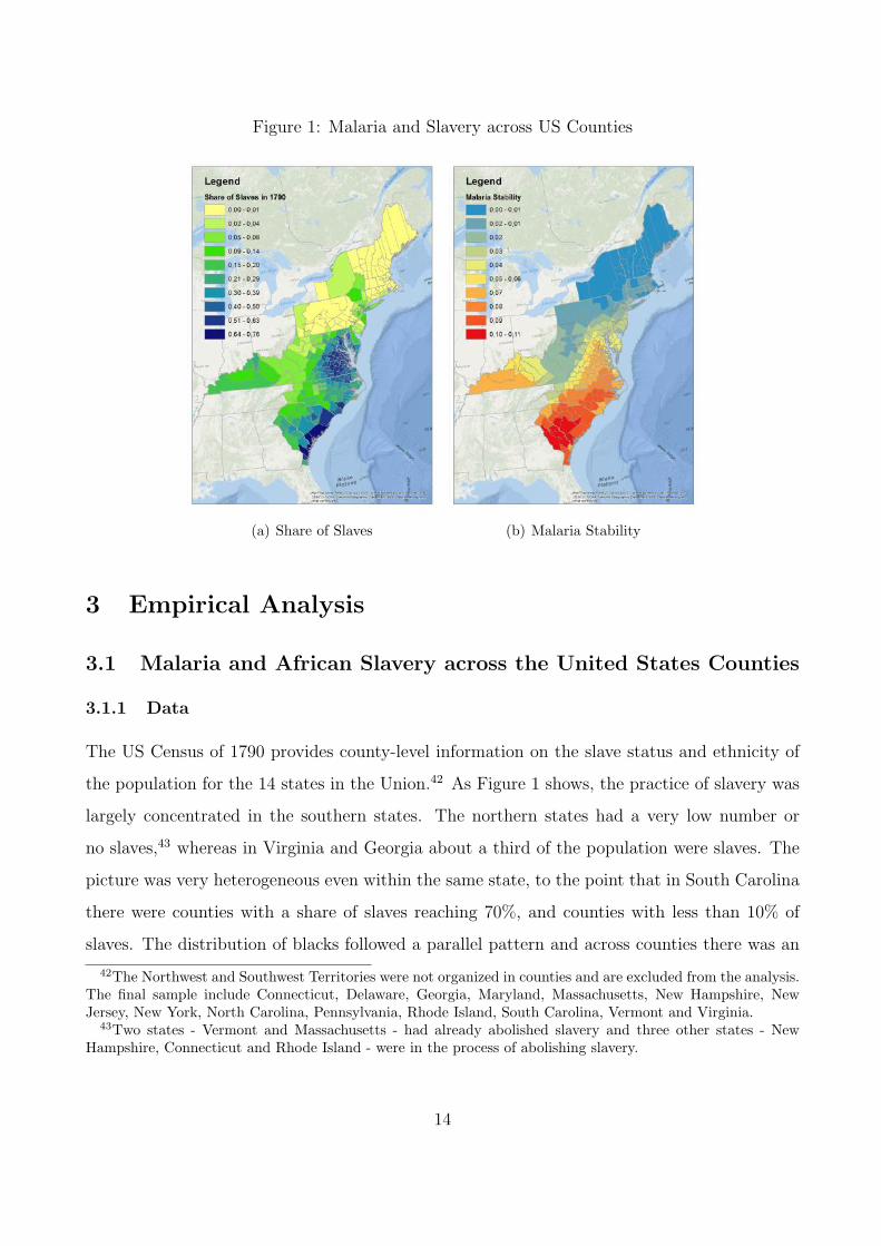
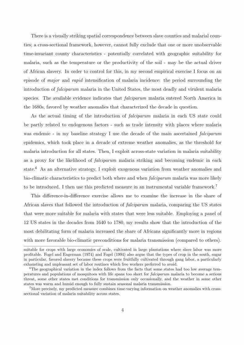
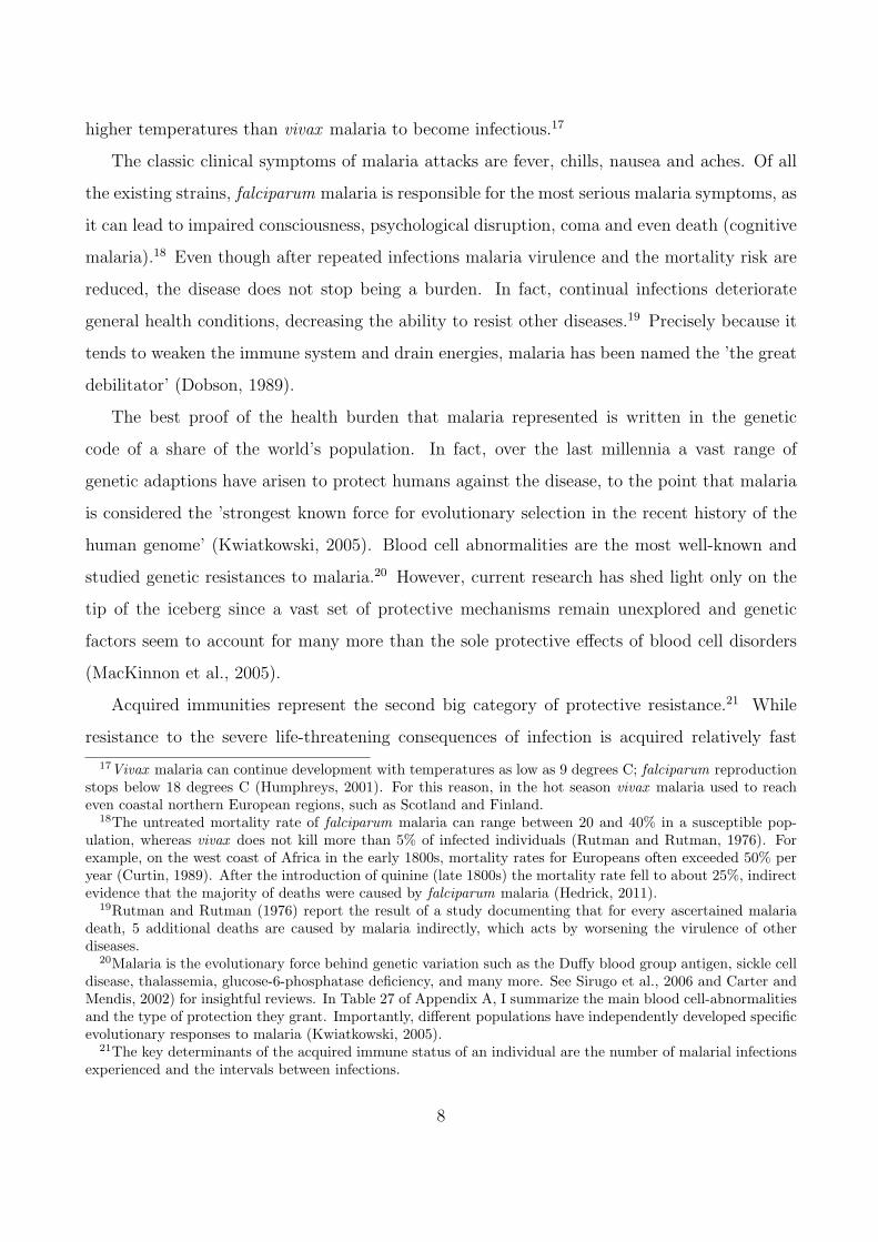
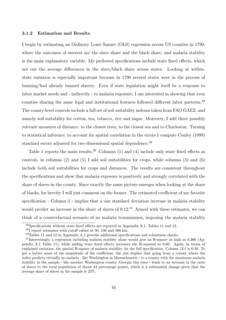
Figure 1: Malaria and Slavery across US Counties

(a) Share of Slaves (b) Malaria Stability

3 Empirical Analysis

3.1 Malaria and African Slavery across the United States Counties

3.1.1 Data

The US Census of 1790 provides county-level information on the slave status and ethnicity of

the population for the 14 states in the Union.42 As Figure 1 shows, the practice of slavery was

largely concentrated in the southern states. The northern states had a very low number or

no slaves,43 whereas in Virginia and Georgia about a third of the population were slaves. The

picture was very heterogeneous even within the same state, to the point that in South Carolina

there were counties with a share of slaves reaching 70%, and counties with less than 10% of

slaves. The distribution of blacks followed a parallel pattern and across counties there was an

42The Northwest and Southwest Territories were not organized in counties and are excluded from the analysis.The final sample include Connecticut, Delaware, Georgia, Maryland, Massachusetts, New Hampshire, NewJersey, New York, North Carolina, Pennsylvania, Rhode Island, South Carolina, Vermont and Virginia.

43Two states - Vermont and Massachusetts - had already abolished slavery and three other states - NewHampshire, Connecticut and Rhode Island - were in the process of abolishing slavery.

14

almost one-to-one correlation between the share of blacks and the share of slaves.44

Turning to malaria distribution, ideally I would require a historical measure of the malaria

incidence across the United States counties in 1790. Unfortunately, accurate measures of

malaria morbidity and mortality for 1790 are unavailable and, most importantly, morbidity

and mortality are themselves a consequence of living standards, agricultural productivity and

other features that might be related to colonizers’ labor choices. Since malaria transmission can

take place only in specific climatic and biological environments, to proxy for effective historical

malaria exposure I exploit an exogenous predicted measure of incidence devised by Kiszewski

et al. (2004): the Malaria Stability Index. This index predicts the risk of being infected

with malaria is as a function of characteristics of the mosquito vector prevalent in the region

- the proportion biting people and the daily survival rate - and climate - a combination of

temperature and precipitation conditions.45 Moreover, I also use a historical index of malaria

endemicity measured at the beginning of the twentieth century, produced by Lysenko (1968)

and digitalized by Hay S.I. (2004).46 The index aims to measure the historical average parasiti-

zation rate at a geographically disaggregated level and offers the advantage of measuring actual

malaria incidence at a time that predates large-scale public health interventions for malaria

eradication.47

44All Europeans and European descendants were classified as “Whites”, while “non-Whites” were people ofAfrican ancestry, or mixed African ancestry. Note that until 1860 the census did not include non-taxed AmericanIndians (i.e. living in tribal society), who composed the great majority of the Native American population.

45Malaria risk is a non-linear function of both temperature and precipitation. Temperature has a hump-shaped effect on malaria risk and the risk is present only when the precipitation level in the previous monthis higher than a threshold. The average risk is computed for each month of the year, and then averaged outinto a cross-sectional variable. The final index has a spatial resolution of 0.5 x 0.5 degrees and ranges from 0 to39. The climatic data employed are averages of monthly observations between 1901 and 1990. Ideally, for myapplication the index should rely on historical climatic data, which are, however, not available for US countiesin 1790. As long as the outcome variables - share of slaves and share of blacks - did not have an influence ontemperature and precipitation, the results are not driven by this aspect of the index.

46In a previous version of this paper, Esposito (2013), I exploited a predicted index of malaria risk devisedby Hong (2007). The index by Hong (2007) is constructed on the basis of several climatic and geographiccharacteristics and of the share of land cleared for agriculture. Since the share of land cleared for agriculturemight capture features of the county with a direct effect on the dependent variables of my study, it is less suitedfor my specific application. Note, however, that the index would give virtually identical results.

47The measure goes from 0, no transmission, to 5 holoendemic (transmission occurs all year long). Theintermediate steps are epidemic, hypoendemic (very intermittent transmission), hyperendemic (intense, butwith periods of no transmission) and mesoendemic (regular seasonal transmission).

15

3.1.2 Estimation and Results

I begin by estimating an Ordinary Least Square (OLS) regression across US counties in 1790,

where the outcomes of interest are the slave share and the black share, and malaria stability

is the main explanatory variable. My preferred specifications include state fixed effects, which

net out the average differences in the slave/black share across states. Looking at within-

state variation is especially important because in 1790 several states were in the process of

banning/had already banned slavery. Even if state legislation might itself be a response to

labor market needs and - indirectly - to malaria exposure, I am interested in showing that even

counties sharing the same legal and institutional features followed different labor patterns.48

The county-level controls include a full set of soil suitability indexes taken from FAO GAEZ, and

namely soil suitability for cotton, tea, tobacco, rice and sugar. Moreover, I add three possibly

relevant measures of distance: to the closest river, to the closest sea and to Charleston. Turning

to statistical inference, to account for spatial correlation in the errors I compute Conley (1999)

standard errors adjusted for two-dimensional spatial dependence.49

Table 1 reports the main results.50 Columns (1) and (4) include only state fixed effects as

controls, in columns (2) and (5) I add soil suitabilities for crops, while columns (3) and (6)

include both soil suitabilities for crops and distances. The results are consistent throughout

the specifications and show that malaria exposure is positively and strongly correlated with the

share of slaves in the county. Since exactly the same picture emerges when looking at the share

of blacks, for brevity I will just comment on the former. The estimated coefficient of my favorite

specification - Column 3 - implies that a one standard deviation increase in malaria stability

would predict an increase in the share of slaves of 0.12.51 Armed with these estimates, we can

think of a counterfactual scenario of no malaria transmission, imposing the malaria stability

48Specifications without state fixed effects are reported in Appendix A.1, Tables 11 and 12.49I report estimates with cutoff values at 50, 100 and 500 km.50Tables 11 and 12 in Appendix A.1 provide additional specifications and robustness checks.51Interestingly, a regression including malaria stability alone would give an R-square as high as 0.366 (Ap-

pendix A.1 Table 11), while adding state fixed effects increases the R-squared to 0.60. Again, in terms ofexplained variation, the partial R-square of malaria stability (in the full specification, Column (3)) is 0.39. Toget a better sense of the magnitude of the coefficient, the size implies that going from a county where theindex predicts virtually no malaria - like Washington in Massachusetts - to a county with the maximum malariastability in the sample - like another Washington county, Georgia this time - leads to an increase in the ratioof slaves to the total population of about 44 percentage points, which is a substantial change given that theaverage share of slaves in the sample is 22%.

16

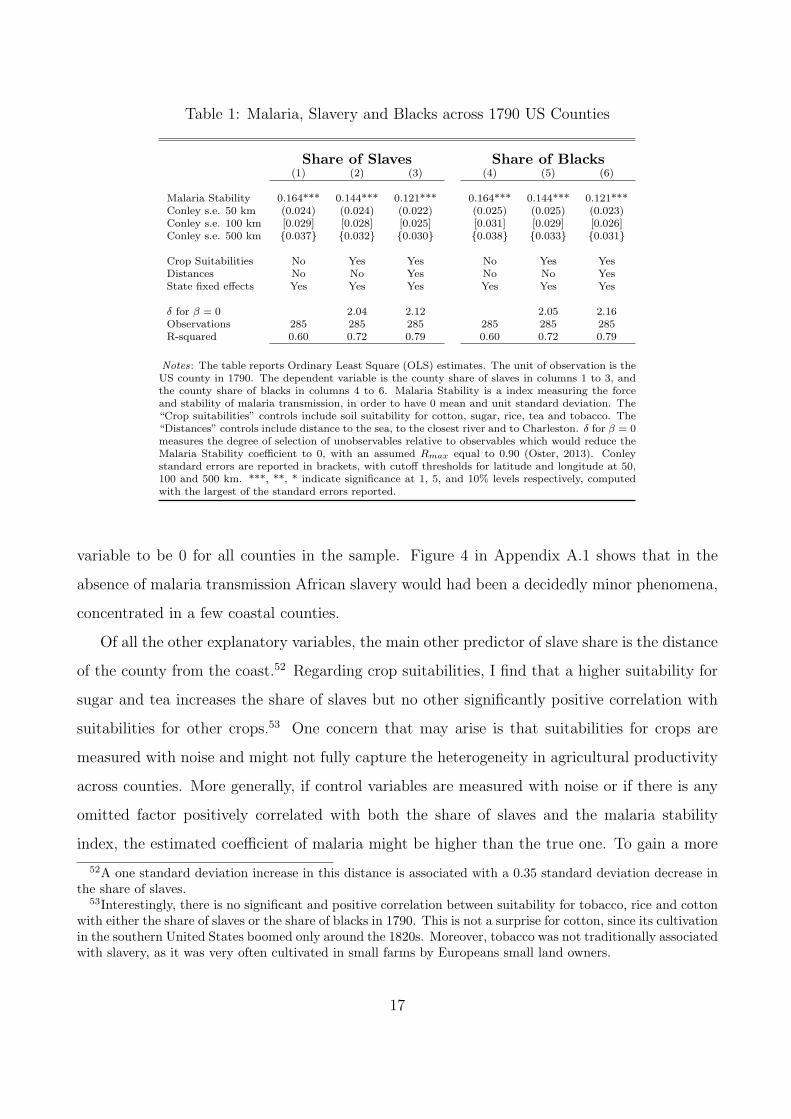
Table 1: Malaria, Slavery and Blacks across 1790 US Counties

Share of Slaves Share of Blacks(1) (2) (3) (4) (5) (6)

Malaria Stability 0.164*** 0.144*** 0.121*** 0.164*** 0.144*** 0.121***Conley s.e. 50 km (0.024) (0.024) (0.022) (0.025) (0.025) (0.023)Conley s.e. 100 km [0.029] [0.028] [0.025] [0.031] [0.029] [0.026]Conley s.e. 500 km {0.037} {0.032} {0.030} {0.038} {0.033} {0.031}

Crop Suitabilities No Yes Yes No Yes YesDistances No No Yes No No YesState fixed effects Yes Yes Yes Yes Yes Yes

δ for β = 0 2.04 2.12 2.05 2.16Observations 285 285 285 285 285 285R-squared 0.60 0.72 0.79 0.60 0.72 0.79

Notes: The table reports Ordinary Least Square (OLS) estimates. The unit of observation is theUS county in 1790. The dependent variable is the county share of slaves in columns 1 to 3, andthe county share of blacks in columns 4 to 6. Malaria Stability is a index measuring the forceand stability of malaria transmission, in order to have 0 mean and unit standard deviation. The“Crop suitabilities” controls include soil suitability for cotton, sugar, rice, tea and tobacco. The“Distances” controls include distance to the sea, to the closest river and to Charleston. δ for β = 0measures the degree of selection of unobservables relative to observables which would reduce theMalaria Stability coefficient to 0, with an assumed Rmax equal to 0.90 (Oster, 2013). Conleystandard errors are reported in brackets, with cutoff thresholds for latitude and longitude at 50,100 and 500 km. ***, **, * indicate significance at 1, 5, and 10% levels respectively, computedwith the largest of the standard errors reported.

variable to be 0 for all counties in the sample. Figure 4 in Appendix A.1 shows that in the

absence of malaria transmission African slavery would had been a decidedly minor phenomena,

concentrated in a few coastal counties.

Of all the other explanatory variables, the main other predictor of slave share is the distance

of the county from the coast.52 Regarding crop suitabilities, I find that a higher suitability for

sugar and tea increases the share of slaves but no other significantly positive correlation with

suitabilities for other crops.53 One concern that may arise is that suitabilities for crops are

measured with noise and might not fully capture the heterogeneity in agricultural productivity

across counties. More generally, if control variables are measured with noise or if there is any

omitted factor positively correlated with both the share of slaves and the malaria stability

index, the estimated coefficient of malaria might be higher than the true one. To gain a more

52A one standard deviation increase in this distance is associated with a 0.35 standard deviation decrease inthe share of slaves.

53Interestingly, there is no significant and positive correlation between suitability for tobacco, rice and cottonwith either the share of slaves or the share of blacks in 1790. This is not a surprise for cotton, since its cultivationin the southern United States boomed only around the 1820s. Moreover, tobacco was not traditionally associatedwith slavery, as it was very often cultivated in small farms by Europeans small land owners.

17

formal insight into the size of this bias, following Oster (2013), I compute how important the

unobservable characteristics of the county should be relative to the observable ones for the

estimated effect of malaria stability to fall down to 0. The results, reported in Table 1, show

that for the true effect of malaria stability to be 0, there should be an effect of unobservables

about 2 times as large as the effect of the observed set of controls (Column 3).54

Looking at other outcomes, higher malaria incidence predicts also a larger share of white

families owning slaves out of all families, and a larger black population measured in absolute

terms (Appendix A.1 Table 10, Panel A). Moreover, the results are robust to the inclusion

of climatic controls such as temperature and precipitation, as well as when holding constant

the total county population (Appendix A.1 Table 10, Panel B). Note that the results are

identical when using the alternative measure of historical malaria incidence, with the estimated

coefficients remarkably similar to the baseline ones (Appendix A.1 Table 11, Panel C ). Finally,

if we were to look only at “slave states”, states where slavery was legally sanctioned in 1790,

we would again find the same identical estimated coefficients (Appendix A.1 Table 11, Panel

D).

3.2 The Introduction of Falciparum Malaria into the Colonies

3.2.1 Empirical Strategy

The cross-sectional results may be fundamentally flawed if the areas where malaria occurred

were different from other areas along dimensions that we do not observe, which could be the ac-

tual reason for greater exploitation of African slaves. To exclude this, I propose an identification

strategy that looks at a change in malaria intensity, by exploiting as a quasi-natural experiment

the introduction of falciparum malaria, the most virulent and deadly malaria species, into the

United States.

The first challenge of the exercise is to identify the exact timing of the introduction of

falciparum malaria into the US colonies. Indeed, thanks to historical evidence, the introduction

of the disease can be dated with a sufficient degree of accuracy. In fact, epidemiology would

54The reported δ are computed assuming an Rmax equal to 0.9. Note, however, that for any assumed valueof Rmax, δ is always larger than 1.5, which is reassuring given that Oster (2013) indicates 1 as a reasonableheuristic value.

18

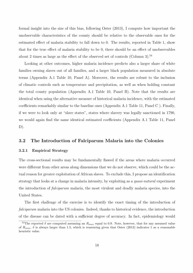
Table 2: Health Changes in South Carolina

Year Source Opinion on the Health of the Colonies

1674 Joseph West, letter to Lord Ashley Our people (God be praised) doe continue very well in healthand the country seemes to be very healthfull and delightsome.

1681 Thomas Newe, letter to his father ...most have a seasoning, but few dye of it.

1684 Lord Cardross and William Dunlop,leaders of the Scottish contingent Car-olina Merchant

We found the place so extraordinarily sicklies that sicknessquickley seased many of our number and took away greatmany...

1737 Immigrant from Europe I herewith wish to have everybody warned that he should nothanker to come into this country, for diseases here have toomuch sway and people have died in masses.

suggest that when a falciparum malaria infection hits a population never previously exposed

to the parasite, violent epidemics must follow. Epidemics are expected to hit until a new

equilibrium is reached, when falciparum malaria starts to be endemic to the region. In effect,

a series of epidemics started to hit the most southern US colonies during the 1680s. The most

well-known is the one that hit Charleston in 1684 (Waring, 1975). An increase in the virulence

and mortality of fevers and agues was registered in various places and the epidemic forms that

the infection took at first, coupled with the sudden rise in the mortality rates that followed,

are consistent with the traits of falciparum malaria.55

Exploring anecdotal evidence with these epidemiological considerations in mind leads Wood

(1974) and Rutman and Rutman (1976) to date the introduction of falciparum malaria around

the mid-1680s. I further conjecture that the weather anomalies that characterized the decade

created weather conditions particularly suitable for the introduction of falciparum malaria. In

fact, based on data that climate historians have pieced together, starting from the 1680s we

observe an increase in extreme weather events.56 Importantly, there is vast anecdotal evidence

documenting a sudden deterioration in the health environment of the Southern colonies in the

1680s. Table 2, for instance, reports extracts for South Carolina before and after the falciparum

epidemic that hit Charleston in 1684.

55See, for instance, Wood (1974); Childs (1940) for South Carolina and Rutman and Rutman (1976) forVirginia.

56El Nino events were documented in 1681, 1683-1684 and 1687-88. For comparison, note that in the twoprevious decades we have evidence of only one El Nino event (1671) in the 1670s, and one event in the 1660s(1661). Figure 5 plots the full time series of El Nino events. Extreme weather events can increase malaria riskin many ways, for instance by creating additional mosquito-breeding places. An exceptionally dry summer canincrease the pools of stagnant water in a river, and unusually heavy rains and floods can do the same.

19

Ideally, the analysis would require information on the specific timing of the introduction

of falciparum malaria into each US state. However, while historical analysis of the health

environment of the major colonial states are vast and informative, smaller and more peripheral

states have received less investigation. Moreover, the actual timing of the introduction of the

disease into each state could itself be a consequence of endogenous factors, such as a larger

prior importation of workers from tropical areas where the disease was already endemic.57

To overcome data limitations and the potential source of endogeneity that might drive the

actual timing of the introduction in different states, in my baseline analysis I use the same date

of falciparum malaria arrival for all states. Based on the work of Wood (1974) and Rutman

and Rutman (1976), I consider the decades up to 1680 (included) as prior to introduction, and

the subsequent decades as post-introduction. Moreover, I exploit the differential geographic

suitability for malaria across states to predict where malaria was more likely to hit and then

become endemic. In a dif-in-dif exercise, I examine the effect of the falciparum shock on the

change in the share of blacks before and after 1690, comparing the states where falciparum

malaria could thrive with the states where it could not.

The main threat to this strategy is posed by shocks that differentially affected states more or

less suitable for malaria and were contemporaneous to the introduction of falciparum malaria.

Drawing on the most popular explanations provided by historians for the rapid switch towards

African labor in high-malaria states, I show that the effect is not driven by the confounding

effects of factors highlighted by the competing hypotheses.

According to several authors, the rapid increase in African labor in the colonies followed

the introduction of a specific variety of rice, the cultivation methods of which were mastered

by people from certain African regions.58 To take into account the possible effect of a surge in

57In other words, we can conceptualize the likelihood of falciparum malaria arriving in the colonies as afunction of two sets of factors: i) the exogenous likelihood related to the bio-climatic conditions, as the arrivalof a falciparum malaria carrier in a cold state where conditions for transmission are not met or met only rarelywas less likely to generate epidemics than the arrival of the carrier in a state where the bio-climatic conditionsfor transmission are frequently met; ii) the endogenous components affecting the probability of introduction,like for instance the size of the workforce from places where malaria was endemic.

58Around 1685 Captain John Thurber introduced a particular variety of rice in Charleston: ’Gold Seede’ fromMadagascar, which happened to prosper in the soils of South Carolina. According to other sources, bushels ofrice were sent to Carolina earlier on. What we know for sure are the bushels of rice exported to England fromthe US colonies. The figures are available from 1698. The rice exported from the producing areas was still verylittle in 1698, with 10,407 pounds of rice exported. However, exports started increasing fast so that in 1700the colonies exported 394,130 pounds of rice. In 1750, the amount of rice exported was over 27 million pounds.

20

rice cultivation on the share of African labor, I allow for a different effect of the state average

suitability for rice before and after 1690, in an exercise which mirrors my main specification

where malaria stability is the variable of interest.59

An alternative explanation behind the rise in African labor in the US colonies centers around

the role played by English wages. While the prices of African slaves remained relatively stable

in the second half of the seventeenth century, the price of servants increased notably due to

a rise in wages registered in England, which pushed up the opportunity costs of Europeans

willing to migrate to the colonies (Galenson, 1981). If the effect of a reduced supply of servants

homogeneously affected all the states in my sample, accounting for aggregate shocks hitting all

the colonies at once would eliminate this potential bias. Furthermore, to exclude the possibility

that the lower availability of European servants affected certain states more than others, I allow

the time series of farm wages in England to affect each state differently.

As an alternative strategy, in order to get rid of the endogeneity that might drive the timing

and location of falciparum malaria introduction, I use time and state variation in bio-climatic

characteristics to predict when and where falciparum malaria became endemic. The predictor is

constructed on the intuition that weather anomalies created conditions favoring the introduction

of falciparum malaria, particularly in states with a higher bio-climatic potential for malaria

transmission. Therefore, as a source of bio-climatic variation I exploit the interaction between

a time-series of weather anomalies (common for all states) and the cross-sectional variation in

malaria suitability across states.60 As a second step, I collect all available information on the

appearance of falciparum malaria for each state and instrument it with my predicted index.

A concern that may arise is the possibility that the falciparum malaria epidemics observed

were a consequence of the greater inflow of Africans in high malaria states, and not viceversa.

Note that both the identification strategies are intended to tackle this concern. First, my

baseline exercise resembles a reduced form specification in spirit. In other words, the inflow

of workers from malaria-infested areas certainly increased the likelihood of epidemics, but the

Source: Colonial and Prefederal Statistics, Chapter Z.59As a robustness exercise, without imposing any structure, I control for a time-varying effect of the average

suitability for rice (and of a set of cash crops) of the state on the share of blacks.60More formally, my exogenous predictor be the term El Ninot ∗MSc, the interaction term between the

number of El Nino events in the decade, which varies by decade, and the malaria stability index in the state,which varies across states.

21

interaction between the post-introduction variable (equal for all states) and the malaria stability

index only exploits exogenous variation in bio-climatic suitability to malaria - i.e. it is not an

actual measure of malaria incidence. Furthermore, in my second strategy I indeed use an

actual measure of incidence - indicating where and when falciparum malaria was endemic - but

I instrument this variable with a predicted measure constructed on the basis of bio-climatic

information.61

3.2.2 Data

The Colonial and Pre-Federal Statistics of the US Census provide figures on the number of

“Whites” and “Negroes” in each state over the decades from the early days of settlement. As

first outcome variable, I look at the average share of blacks in the total population of the state.

As a second outcome of interest, I investigate when and in which US states the southern slave

labor system was institutionalized. Until the last decades of the seventeenth century, in fact,

Africans in the United States were treated similarly as servants from England, Scotland, Ireland

and Native Americans.62 Then, in the last decades of the seventeenth century “... Negroes did

cease to be servants and became slaves”: Africans became property of their owners, for life.63

The stiffening of the legislation governing living and working conditions of Africans culminated

into the approval of comprehensive “slave codes” in some of the US states. For my analysis,

I employ the approval of a “slave code” as a proxy for the apex in the reduction of liberties

experienced by Africans employed in each state.

In my final sample, where the unit of observation is the state at the beginning of each

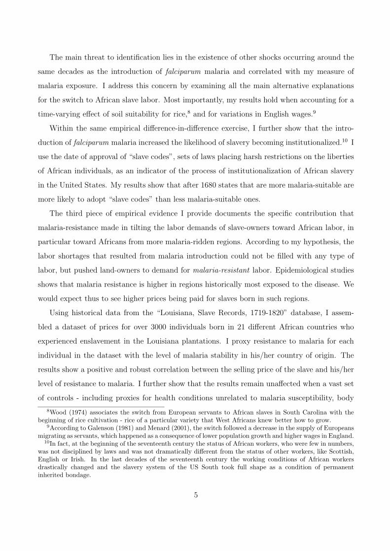
decade, I observe 12 states from 1640 to 1780.64 Figure 2 summarizes the evolution of the share

61Note, however, that according to my hypothesis there is indeed scope for path-dependence in the mechanismwhich led to the establishment of African slavery in the southern US. In fact, bringing Africans to states wheremalaria can take root could have increased the likelihood of acquiring malaria, which then might have furtherenhanced the need for African workers. Even according to this version of the hypothesis, the primary driverremains malaria.

62“The status of Negroes was that of servants” (Oscar and Handlin, 1950).63As Oscar and Handlin (1950) put it “slavery was not there from the start...”, and it was in the last decades

of the seventeenth century that “Negroes did cease to be servants and became slaves, ceased to be men in whommasters held a proprietary interest and became chattels, objects that were the property of their owners. In thattransformation originated the Southern labor system.”.

64I exclude 1630, as information for only 4 states was available. However, the results would not change if Iwere to include 1630 in the sample. Moreover, as they would not contribute to the empirical analysis, I excludestates that are observed only after 1690. Moreover, to be able to compare data over time I consider Maine,Playmouth and Massachusetts as a single state.

22

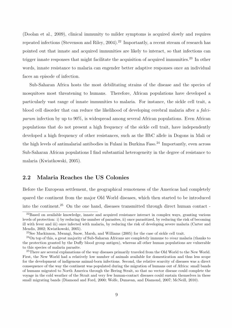
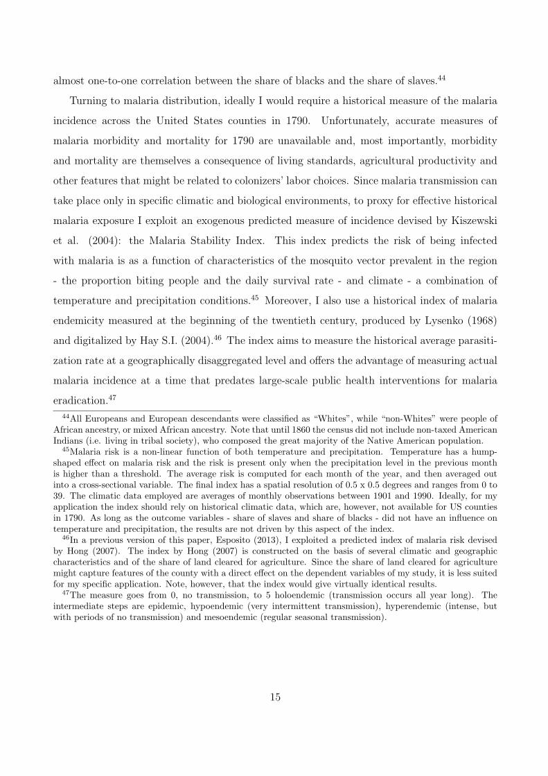
Figure 2: Blacks over Total Population in US Colonies

0.2

.4.6

.8B

lack

s to

Tot

al P

opul

atio

n

1650 1700 1750 1800Years

South Carolina North CarolinaVirginia MarylandDelaware New JerseyPennsylvania ConnecticutRhode Island New HampshireNew York Massachusetts

†The graphs show the ratio of Africans to the total population in the US pre-federal states. The line is black for all states with a

malaria stability index higher than the average and grey for all states with an index below the average.

23

of Africans over time across the 12 states in the sample.

I use the malaria stability index of Kiszewski et al. (2004) to proxy for the average geo-

graphical suitability for malaria in the state.65 In Figure 2, states with higher than average

malaria stability are reported in black and lower than average malaria stability states are in

light grey. Before 1690, the high-malaria states had average shares of blacks only slightly higher

than the low-malaria states: respectively 6% and 4%. After 1690, the two groups of states took

diverging paths, with the low-malaria states states maintaining the same low share of blacks

(around 5%), while in the high-malaria states blacks reached on average 27% of the total popu-

lation. Furthermore, I find that until the 1680s no state had a slave code in force, while starting

in the 1690s more than half of the states approved a slave code.66

3.2.3 Estimation and Results

Figure 2 seems to suggest that after 1690 the share of blacks in the population jumped rapidly

only in the more malaria-suitable states. Turning to a more formal analysis, I propose a set of

estimates based on the specification below:

%Blacks,t = α + β ∗MSs ∗ Post1690t +n∑i=1

γ ∗ Is,t + µs + µt + εs,t (1)

The main interest lies in β, the coefficient of the interaction term between Post-1690t, an

indicator taking value 1 for the decades following 1690 (with 1690 included), and the variable

MSs, which is a continuous index measuring malaria stability in the state standardized in

order to have 0 mean and unit standard deviation. All the specifications include state fixed

effects µs and decade fixed effects µt, with the aim to net out variation arising from time-

invariant differences across states and shocks common to all states. The main outcome of

interest is %Blacks,t, the share of black population in the state at the beginning of the decade.67

65As a robustness check, I employ the historical index of malaria endemicity measured at the beginningof the twentieth century. The index contains relevant information as long as the malaria distribution at thebeginning of the twentieth century is a function of bio-climatic conditions already present during the colonialtimes. However, if the distribution of African slaves affected the malaria endemicity rate at the beginning ofthe twentieth century, the results might be biased and need to be interpreted with caution.

66Note that, given that the treatment is continuous, I cannot provide the standard difference-in-differencegraphical representation mapping treated and not treated.

67Ideally, I would like to identify the same diverging paths in the time series of wages for free workers, whichat the time were primarily European servants. In other words, I expect to observe a higher cost for free labor

24

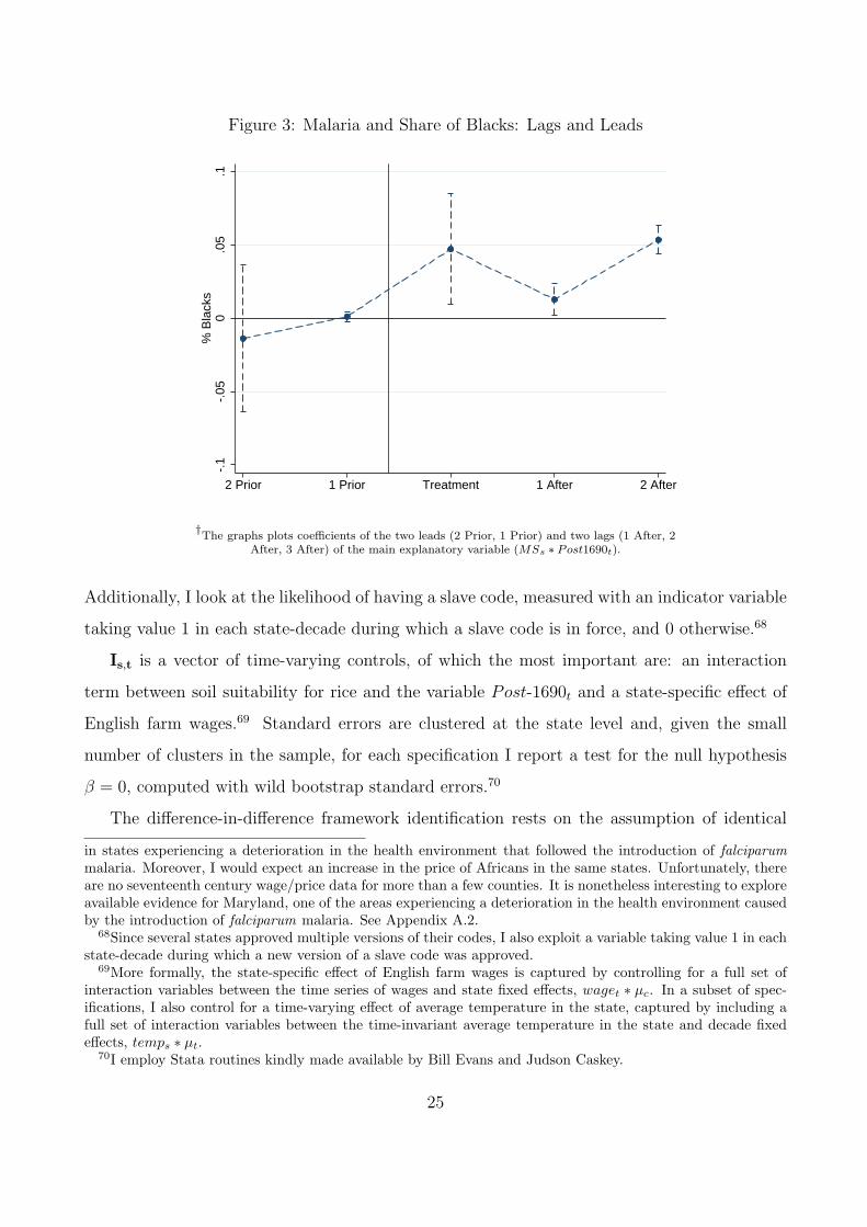
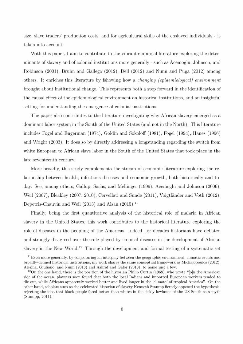
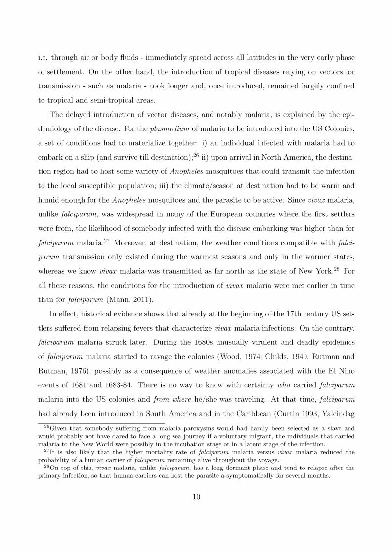
Figure 3: Malaria and Share of Blacks: Lags and Leads

-.1

-.05

0.0

5.1

% B

lack

s

2 Prior 1 Prior Treatment 1 After 2 After

†The graphs plots coefficients of the two leads (2 Prior, 1 Prior) and two lags (1 After, 2

After, 3 After) of the main explanatory variable (MSs ∗ Post1690t).

Additionally, I look at the likelihood of having a slave code, measured with an indicator variable

taking value 1 in each state-decade during which a slave code is in force, and 0 otherwise.68

Is,t is a vector of time-varying controls, of which the most important are: an interaction

term between soil suitability for rice and the variable Post-1690t and a state-specific effect of

English farm wages.69 Standard errors are clustered at the state level and, given the small

number of clusters in the sample, for each specification I report a test for the null hypothesis

β = 0, computed with wild bootstrap standard errors.70

The difference-in-difference framework identification rests on the assumption of identical

in states experiencing a deterioration in the health environment that followed the introduction of falciparummalaria. Moreover, I would expect an increase in the price of Africans in the same states. Unfortunately, thereare no seventeenth century wage/price data for more than a few counties. It is nonetheless interesting to exploreavailable evidence for Maryland, one of the areas experiencing a deterioration in the health environment causedby the introduction of falciparum malaria. See Appendix A.2.

68Since several states approved multiple versions of their codes, I also exploit a variable taking value 1 in eachstate-decade during which a new version of a slave code was approved.

69More formally, the state-specific effect of English farm wages is captured by controlling for a full set ofinteraction variables between the time series of wages and state fixed effects, waget ∗ µc. In a subset of spec-ifications, I also control for a time-varying effect of average temperature in the state, captured by including afull set of interaction variables between the time-invariant average temperature in the state and decade fixedeffects, temps ∗ µt.

70I employ Stata routines kindly made available by Bill Evans and Judson Caskey.

25

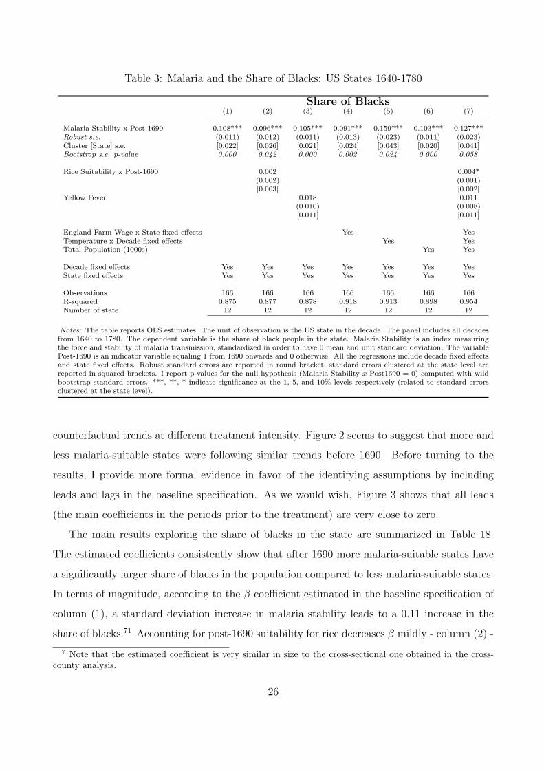
Table 3: Malaria and the Share of Blacks: US States 1640-1780

Share of Blacks(1) (2) (3) (4) (5) (6) (7)

Malaria Stability x Post-1690 0.108*** 0.096*** 0.105*** 0.091*** 0.159*** 0.103*** 0.127***Robust s.e. (0.011) (0.012) (0.011) (0.013) (0.023) (0.011) (0.023)Cluster [State] s.e. [0.022] [0.026] [0.021] [0.024] [0.043] [0.020] [0.041]Bootstrap s.e. p-value 0.000 0.042 0.000 0.002 0.024 0.000 0.058

Rice Suitability x Post-1690 0.002 0.004*(0.002) (0.001)[0.003] [0.002]

Yellow Fever 0.018 0.011(0.010) (0.008)[0.011] [0.011]

England Farm Wage x State fixed effects Yes YesTemperature x Decade fixed effects Yes YesTotal Population (1000s) Yes Yes

Decade fixed effects Yes Yes Yes Yes Yes Yes YesState fixed effects Yes Yes Yes Yes Yes Yes Yes

Observations 166 166 166 166 166 166 166R-squared 0.875 0.877 0.878 0.918 0.913 0.898 0.954Number of state 12 12 12 12 12 12 12

Notes: The table reports OLS estimates. The unit of observation is the US state in the decade. The panel includes all decadesfrom 1640 to 1780. The dependent variable is the share of black people in the state. Malaria Stability is an index measuringthe force and stability of malaria transmission, standardized in order to have 0 mean and unit standard deviation. The variablePost-1690 is an indicator variable equaling 1 from 1690 onwards and 0 otherwise. All the regressions include decade fixed effectsand state fixed effects. Robust standard errors are reported in round bracket, standard errors clustered at the state level arereported in squared brackets. I report p-values for the null hypothesis (Malaria Stability x Post1690 = 0) computed with wildbootstrap standard errors. ***, **, * indicate significance at the 1, 5, and 10% levels respectively (related to standard errorsclustered at the state level).

counterfactual trends at different treatment intensity. Figure 2 seems to suggest that more and

less malaria-suitable states were following similar trends before 1690. Before turning to the

results, I provide more formal evidence in favor of the identifying assumptions by including

leads and lags in the baseline specification. As we would wish, Figure 3 shows that all leads

(the main coefficients in the periods prior to the treatment) are very close to zero.

The main results exploring the share of blacks in the state are summarized in Table 18.

The estimated coefficients consistently show that after 1690 more malaria-suitable states have

a significantly larger share of blacks in the population compared to less malaria-suitable states.

In terms of magnitude, according to the β coefficient estimated in the baseline specification of

column (1), a standard deviation increase in malaria stability leads to a 0.11 increase in the

share of blacks.71 Accounting for post-1690 suitability for rice decreases β mildly - column (2) -

71Note that the estimated coefficient is very similar in size to the cross-sectional one obtained in the cross-county analysis.

26

just like accounting for the state-specific effects of English farm wages - column (5). In column

(3) I account for the number of yellow fever epidemics in the state in the decade, which, however,

leave the coefficient unaffected, just as controlling for the population in the state. Finally, it is

reassuring that the inclusion of temperature interacted with year fixed effects does not reduce,

but actually increases, the size of β, indicating that the the estimated effect is not driven by

pre/post 1690 differences acting along a climatic gradient. In additional specifications, reported

in Tables 16, I show that the effect of stability is not driven by a spurious correlation with cash

crop suitability. First, I interact cash crops suitability with a post-1690 indicator variable,

second, I allow for the effect of soil suitability for rice, tobacco and tea to vary over time,

interacting soil suitabilities with a full set of decade fixed effects. In Panel B of Table 17, as a

robustness exercise, I exclude each of the four southernmost states and show that the results

are not driven by any specific southern state.

Table 4 reports Linear Probability Model (LPM) estimations exploring the distribution

of “slave codes”. In the upper panel the dependent variable, Slave Code in Force, indicates

whether a slave code is in force in the state-decade, whereas in the lower panel the variable Slave

Code Approval indicates whether the state approved a slave code in the decade. The results

show that the falciparum malaria shock increases the likelihood of having a slave code in force,

and of approving one, for highly malaria-suitable states when compared to low malaria-suitable

states.72 As for robustness checks, Panel A of Table 16 shows that results hold when using the

historical malaria endemicity index.

As a second identification strategy, I construct a variable (Falciparum Malaria) indicating

for each state when historical evidence documents falciparum malaria’s appearance. Since

the variable Falciparum Malaria is measured with error and might be endogenously driven

by spurious factors, I instrument it with a variable aiming at capturing the effect of weather

anomalies in more malaria-suitable states. My proxy measure for weather anomalies (common

to all states) is the number of El Nino events registered in the decade.73 The results, summarized

in Table 18, show that: i) weather anomalies in the highly malaria-suitable states significantly

72A standard deviation increase in malaria stability increases by one third the probability of having a slavecode in force.

73More precisely, the instrument is the interaction term between El Nino events #El Ninot and the malariastability in the state MSc.

27

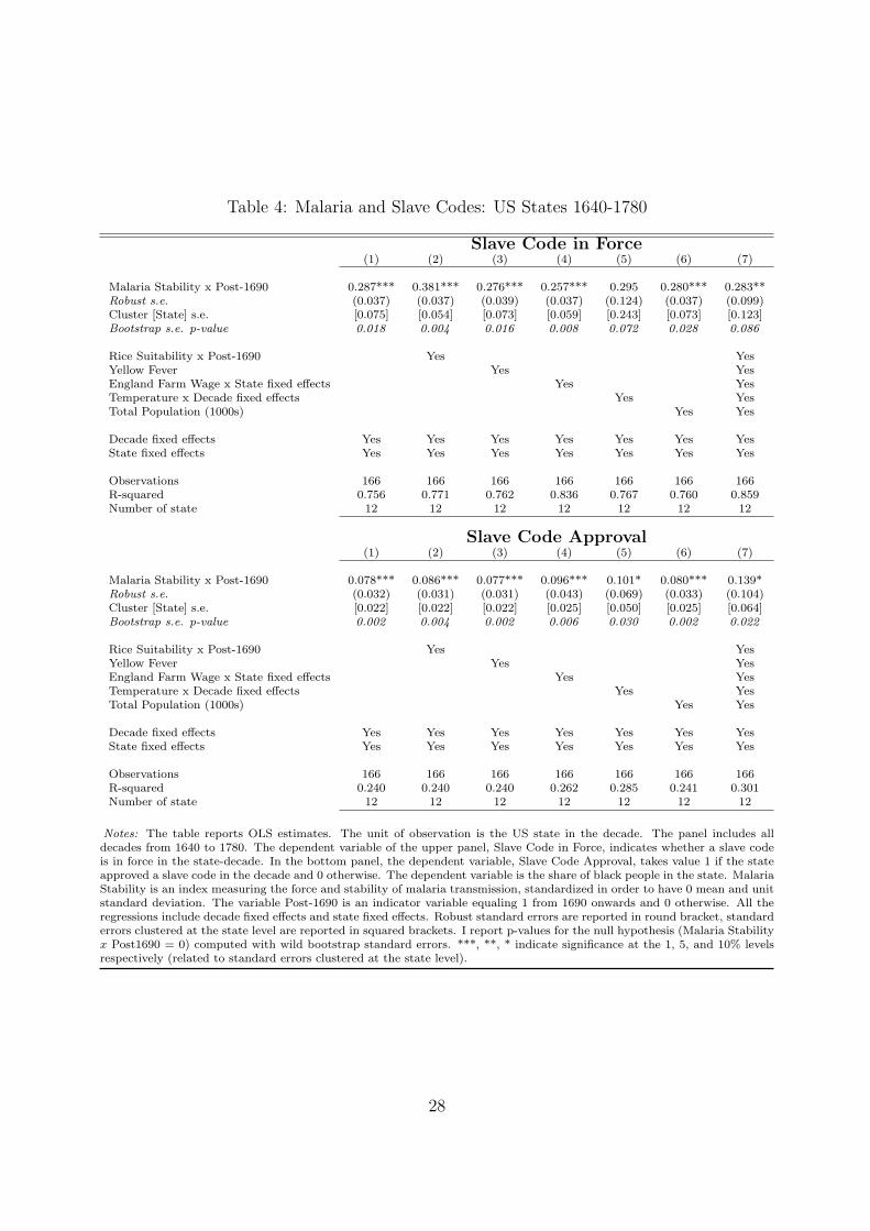
Table 4: Malaria and Slave Codes: US States 1640-1780

Slave Code in Force(1) (2) (3) (4) (5) (6) (7)

Malaria Stability x Post-1690 0.287*** 0.381*** 0.276*** 0.257*** 0.295 0.280*** 0.283**Robust s.e. (0.037) (0.037) (0.039) (0.037) (0.124) (0.037) (0.099)Cluster [State] s.e. [0.075] [0.054] [0.073] [0.059] [0.243] [0.073] [0.123]Bootstrap s.e. p-value 0.018 0.004 0.016 0.008 0.072 0.028 0.086

Rice Suitability x Post-1690 Yes YesYellow Fever Yes YesEngland Farm Wage x State fixed effects Yes YesTemperature x Decade fixed effects Yes YesTotal Population (1000s) Yes Yes

Decade fixed effects Yes Yes Yes Yes Yes Yes YesState fixed effects Yes Yes Yes Yes Yes Yes Yes

Observations 166 166 166 166 166 166 166R-squared 0.756 0.771 0.762 0.836 0.767 0.760 0.859Number of state 12 12 12 12 12 12 12

Slave Code Approval(1) (2) (3) (4) (5) (6) (7)

Malaria Stability x Post-1690 0.078*** 0.086*** 0.077*** 0.096*** 0.101* 0.080*** 0.139*Robust s.e. (0.032) (0.031) (0.031) (0.043) (0.069) (0.033) (0.104)Cluster [State] s.e. [0.022] [0.022] [0.022] [0.025] [0.050] [0.025] [0.064]Bootstrap s.e. p-value 0.002 0.004 0.002 0.006 0.030 0.002 0.022

Rice Suitability x Post-1690 Yes YesYellow Fever Yes YesEngland Farm Wage x State fixed effects Yes YesTemperature x Decade fixed effects Yes YesTotal Population (1000s) Yes Yes

Decade fixed effects Yes Yes Yes Yes Yes Yes YesState fixed effects Yes Yes Yes Yes Yes Yes Yes

Observations 166 166 166 166 166 166 166R-squared 0.240 0.240 0.240 0.262 0.285 0.241 0.301Number of state 12 12 12 12 12 12 12

Notes: The table reports OLS estimates. The unit of observation is the US state in the decade. The panel includes alldecades from 1640 to 1780. The dependent variable of the upper panel, Slave Code in Force, indicates whether a slave codeis in force in the state-decade. In the bottom panel, the dependent variable, Slave Code Approval, takes value 1 if the stateapproved a slave code in the decade and 0 otherwise. The dependent variable is the share of black people in the state. MalariaStability is an index measuring the force and stability of malaria transmission, standardized in order to have 0 mean and unitstandard deviation. The variable Post-1690 is an indicator variable equaling 1 from 1690 onwards and 0 otherwise. All theregressions include decade fixed effects and state fixed effects. Robust standard errors are reported in round bracket, standarderrors clustered at the state level are reported in squared brackets. I report p-values for the null hypothesis (Malaria Stabilityx Post1690 = 0) computed with wild bootstrap standard errors. ***, **, * indicate significance at the 1, 5, and 10% levelsrespectively (related to standard errors clustered at the state level).

28

predict the variable Falciparum Malaria - First Stage, Table 18; ii) weather anomalies in

the more malaria-suitable states are also associated with a sizable increases in the share of

blacks and a higher likelihood of having a slave code in force - Reduced Form, Table 18; iii)

instrumenting the variable Falciparum Malaria with weather anomalies in the more malaria-

suitable states, I find instrumental variable estimates in line with the OLS ones - OLS and IV,

Table 18.

3.3 Malaria Resistance and Slave Prices

Only to the unpracticed eye could all Africans look alike.

– Ullrich Bonnel Philips, American Negro Slavery

Evidence from the previous sections shows that malaria was an important determinant for

the diffusion of African slavery in the southern United States. This section aims to document

that it is precisely the comparative higher malaria-resistance of sub-Saharan Africans that made

them especially attractive for employment in these regions. In other words, this section aims to

show that slave-owners’ labor choices moved from a conscious intent to meet their labor needs

with the comparatively most productive pool of laborers.74

Thus, in this last section I provide evidence of slave-owners’ preferences for slaves with higher

resistance and immunities to malaria. In order to do so, I conjecture that among the African

workers shipped to North America, individuals born in African regions with more malaria had

a higher stock of acquired and innate immunities to the disease. On the premise that malaria

resistance was associated with better health and higher productivity, I search for a malaria

premium in the slave transactions occurring in the Louisiana slave market.

The possibility of detecting a malaria premium in prices depends on the existence of a com-

petitive market for slaves. Fogel and Engerman (1974) claim that slave-owners were rational

profit maximizers who paid a price for their slaves equal to their marginal productivity, properly

discounted. Indeed, Louisiana was a very large slave market with thousands of yearly trans-

actions. Along similar lines, Kotlikoff (1979) shows that selling prices reflected productivity

74In other terms, according to the hypothesis the enslavement of Africans in the US South did not only followfrom labor scarcity in the unhealthy malaria-ridden areas but for a specific quest for malaria-resistant labor.

29

differentials resulting from characteristics such as age, sex and skills.75

Crucially, a large body of anecdotal evidence documents the fact that colonizers preferred

certain African groups over others, and that health played an important role in the shaping

of these preferences.76 Perceptions that individuals born in different African regions fared

differently in the low land plantations of North America are present in planters’ own accounts.

Ibos from the Niger Delta, for instance, were considered sickly, whereas Gold Coast slaves were

seen as hardy, robust and subject to little mortality (Littlefield, 1981).

Planters had limited understanding of the determinants behind these health differentials.

Certain diseases had clearly identifiable symptoms, such as smallpox, while the symptoms of

malaria were more difficult to identify. Notwithstanding the obvious complications in diagnosis

experienced at the time, interesting insights emerge from the details of these perceived differen-

tial health susceptibilities. In the case of Congos, for instance, their higher degree of mortality

was experienced in lowland plantations (Geggus, 2001), and we know that malaria was in fact

the major disease of the lowlands. Furthermore, regarding the peculiar fitness of Gold Coast

slaves, it is mentioned that they “were fit to work immediately”. In other words, they needed

to undergo a less debilitating form of ’seasoning’, the dangerous process of adjustment to the

local set of pathogens that each newcomer had to go through, among which malaria fevers

represented the major component. On top of this, it is important to keep in mind that malaria

tends to weaken the immune system, so that individuals contracting the infection are more

vulnerable to several other diseases.

For the present analysis it is important to acknowledge that the health of individuals en-

slaved from Africa was also influenced by the hardship of the long voyage from their African

country of origin.77 Moreover, slave origin was considered to matter for a vast set of physical

and cultural characteristics beyond health, such as body size and agricultural skills. For in-

75Kotlikoff (1979) estimates a male premium from 23.6% to 48.8%. The polynomial he estimates for agepeaks at age 22. The presence of warranties for a large share of slave transactions is another indicator of therationality and scrutiny that characterized the trade (Kotlikoff, 1979).

76Peter Wood (1974), among many others, asserts that “white colonists would have marveled at the ignoranceof their descendants, who asserted blindly that all Africans looked the same”. Along similar lines, Wax (1973)claims that “slave preferences were apparent in all of the colonies and helped to shape the dimensions andcomposition of the slave trade to the mainland”.

77The direction of the effect of the hardships faced during the long voyage from Africa on individual health isambiguous. On the one hand, the hardship of the voyage might have long-lasting detrimental consequences onhealth; on the other hand we might expect a selection bias effect with the consequence of only the more healthypeople being able to survive to the destination.

30

stance, body size was considered a direct consequence of the food availability and the vegetation

in the regions of birth.78 Moreover, Mauro (1964) points out that slaves “did not arrive naked,

but brought with them a sense of sedentary life and of agriculture”.79

3.3.1 Data

To test my hypothesis, I employ a database collecting records for a large number of individuals

who came to Louisiana as slaves between 1719 and 1820: The “Louisiana, Slave Records”

database, conceived and designed by Gwendolyn Midlo Hall (Hall, 2005). The database contains

a rich set of biographical and genealogical details for thousands of individuals who experienced

slavery in the Louisiana plantations. For the purpose of my analysis, the “Louisiana, Slave

Records” database has the unique feature of documenting for individual slaves born in Africa

both their selling price and their place of birth.80

Reconnecting information on the place of birth as recorded in the database to a geographical

unit is a key part of my analysis. For over half of the individuals in the sample, the place of

birth is defined in terms of “modern countries” or political entities largely overlapping with

modern country borders.81 For about one third of the records, the ethnicity of the slave is

provided, whereas cities or geographical locations are the place of birth indicated for about

10% of individuals.82 I aggregate all the available information at the African country level,

since anecdotal evidence suggests that planters did not have detailed knowledge of the vari-

ous African ethnicities, but tended to refer to broader families or larger geographical/cultural

units.83 Narratives in Wax (1973), who studies US slave-owners’ preferences by place of origin,

78Slaves from the Gold Coast, for instance, had access to a vast set of nutritious foods, whereas people livingon the coast had diets relying mainly on fish, tubers and vegetables (Littlefield, 1981).

79Wood (1974) points to the central role of skills in the cultivation of rice. According to him, slaves fromAfrican “rice” regions were in high demand in places specializing in extensive rice cultivation, like South Carolina.

80Individuals born in Africa represent more than half of the individuals for whom I have details on the place ofbirth. Following the instructions of the author, Hall (2005), I exclude records retrieved from the Atlantic SlaveTrade database, which mixes the place of birth and the place of embarkation of the slave. The choice to excludeslaves for whom I only know the port of embarkation and not the exact place of birth follows from my aim toproxy the endowment of acquired and innate immunities to malaria with the epidemiological environment ofthe place of birth. Note, however, that the results would not change if I included records from the AtlanticSlave Trade database.

81This is no surprise if we look at two historical maps drawn by Europeans in 1808 and 1829, which I provide inthe Appendix. In fact, geographical areas are identified with labels that are easily linkable to modern countriesand that to a large extent overlap with modern country borders.

82For the remaining records, I could not track the recorded place of birth to any geographical location.83For instance, in the two advertisements reported in the Appendix, the slave traders refer to slaves from

31

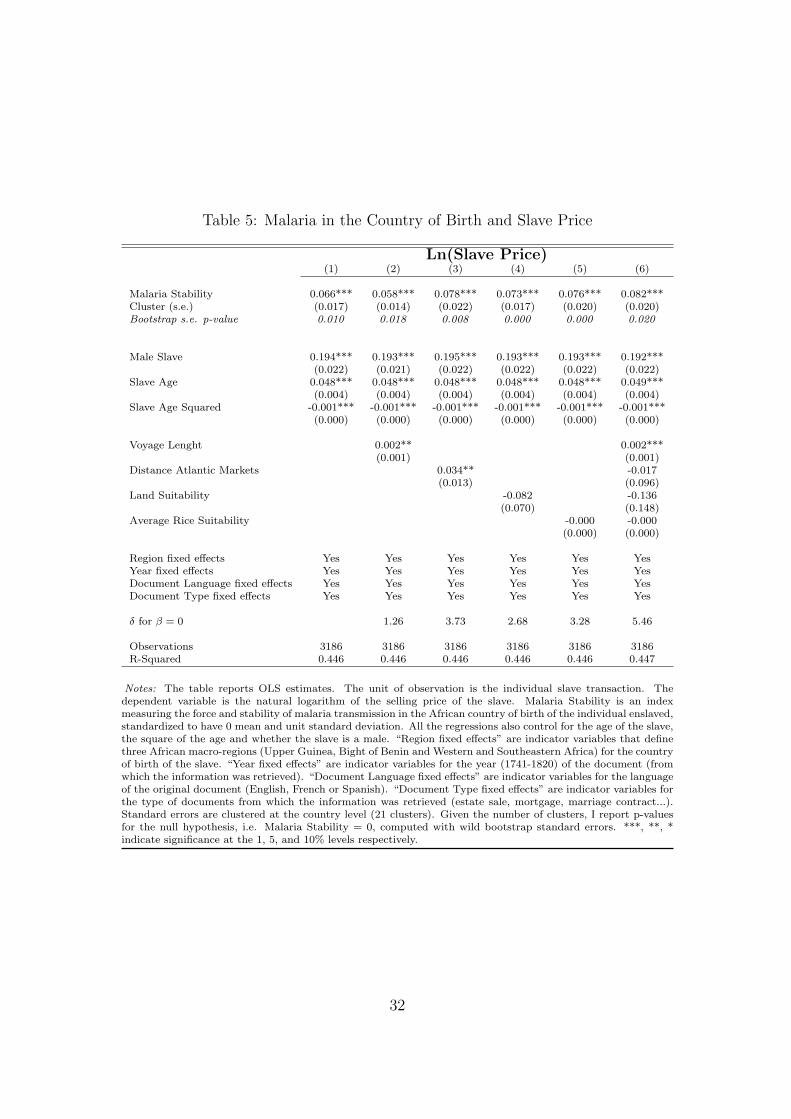
Table 5: Malaria in the Country of Birth and Slave Price

Ln(Slave Price)(1) (2) (3) (4) (5) (6)

Malaria Stability 0.066*** 0.058*** 0.078*** 0.073*** 0.076*** 0.082***Cluster (s.e.) (0.017) (0.014) (0.022) (0.017) (0.020) (0.020)Bootstrap s.e. p-value 0.010 0.018 0.008 0.000 0.000 0.020

Male Slave 0.194*** 0.193*** 0.195*** 0.193*** 0.193*** 0.192***(0.022) (0.021) (0.022) (0.022) (0.022) (0.022)

Slave Age 0.048*** 0.048*** 0.048*** 0.048*** 0.048*** 0.049***(0.004) (0.004) (0.004) (0.004) (0.004) (0.004)

Slave Age Squared -0.001*** -0.001*** -0.001*** -0.001*** -0.001*** -0.001***(0.000) (0.000) (0.000) (0.000) (0.000) (0.000)

Voyage Lenght 0.002** 0.002***(0.001) (0.001)

Distance Atlantic Markets 0.034** -0.017(0.013) (0.096)

Land Suitability -0.082 -0.136(0.070) (0.148)

Average Rice Suitability -0.000 -0.000(0.000) (0.000)

Region fixed effects Yes Yes Yes Yes Yes YesYear fixed effects Yes Yes Yes Yes Yes YesDocument Language fixed effects Yes Yes Yes Yes Yes YesDocument Type fixed effects Yes Yes Yes Yes Yes Yes

δ for β = 0 1.26 3.73 2.68 3.28 5.46

Observations 3186 3186 3186 3186 3186 3186R-Squared 0.446 0.446 0.446 0.446 0.446 0.447

Notes: The table reports OLS estimates. The unit of observation is the individual slave transaction. Thedependent variable is the natural logarithm of the selling price of the slave. Malaria Stability is an indexmeasuring the force and stability of malaria transmission in the African country of birth of the individual enslaved,standardized to have 0 mean and unit standard deviation. All the regressions also control for the age of the slave,the square of the age and whether the slave is a male. “Region fixed effects” are indicator variables that definethree African macro-regions (Upper Guinea, Bight of Benin and Western and Southeastern Africa) for the countryof birth of the slave. “Year fixed effects” are indicator variables for the year (1741-1820) of the document (fromwhich the information was retrieved). “Document Language fixed effects” are indicator variables for the languageof the original document (English, French or Spanish). “Document Type fixed effects” are indicator variables forthe type of documents from which the information was retrieved (estate sale, mortgage, marriage contract...).Standard errors are clustered at the country level (21 clusters). Given the number of clusters, I report p-valuesfor the null hypothesis, i.e. Malaria Stability = 0, computed with wild bootstrap standard errors. ***, **, *indicate significance at the 1, 5, and 10% levels respectively.

32

show that slave-owners referred to the origins of their slaves with terms such as as: Calabari,

Gold Coast, Wydah, Gambia, Angola and Congo slaves.84

The link to modern countries for the majority of the reported places of origin in the sample

is straightforward (for instance Gold Coast, Gabon, Coast of Senegal). I exclude individuals

in the sample with an ethnicity not clearly traceable to a single modern country.85 Moreover,

I perform a vast set of robustness checks, excluding individuals whose place of origin can only

imperfectly be matched to a modern country.

Among the subset of slaves born in Africa, I exclude records for individuals that contain

no price information or that are sold in groups.86 I further exclude individuals with no age

or sex information. For my baseline specifications, I assemble a final sample composed of

3186 individuals sold in the Louisiana Slave Market between 1741 and 1820, with places of

birth spanning 21 African countries.87 Since different slave transactions took place in different

currencies, I exploit the price conversion variable constructed by Robert A. Rosenberg, which

converts all prices into dollar values. The average selling price in the sample is equal to 570 US

dollars. The majority of the transactions involved male individuals, and the average age was

29.

3.3.2 Estimation and Results

Turning to my empirical exercise, I propose the following baseline specification:

ln(price)i,c,r,t = β0 + β1MSc,r + β2Xi,c,r,t + β3Zc,r + µr + µt + εi,c,r,t

where the dependent variable is the natural logarithm of the price for the individual i sold in

year t, born in African country c, located in region r. The main variable of interest is the

Sierra Leon, Windward Coast and Rice Coast.84Hall (2005) claims that - wherever the ethnic origin of the slave was specified - it was an information

provided by the slave him/herself.85In particular, I exclude Manding and Fulani. Note, however, that including them by tracing them to the

country which currently hosts the largest population would leave the results unaffected.86Two types of prices are provided: sale and inventory prices. For my baseline results I use selling prices. If

I included inventory prices, the results would not change. A robustness estimation including all the prices isavailable in the Appendix.

87The countries of origin for the individuals in my sample are Angola, Benin, Burkina Faso, Cameroon,Central African Republic, Congo, Congo Democratic Republic, Cote d’Ivoire, Gabon, Ghana, Guinea, GuineaBissau, Liberia, Mali, Mozambique, Nigeria, Senegal, Sierra Leone, Tanzania, Togo and Zimbabwe.

33

level of malaria stability in the country of origin of the enslaved individual MSc,r. Individual

controls Xi,c,r,t include age, age squared, a dummy variable taking value one if the slave is a

male, type of sale transaction and the language of the document that registered the transaction.

I allow for a non-linear effect of age on prices by including an age squared term. Note that

document type refers to the kind of transaction - i.e. sale, estate sale, seizure for debt - and

allows me to exclude any patterns in slave pricing related to the type of transaction confounding

my results. Equally importantly, since French, Spanish and English slave owners are involved

in the transactions, I include fixed effects for the languages of the document registering the

transaction. On top of this, all the specifications include three African regions fixed effects, to

avoid comparing slaves born in overly distant locations.

Finally, I add an extensive set of country-level controls Zc,r. The first set of controls aims

to proxy for the hardship of the journey from the African country of origin. The second set

of country controls includes several measures of suitability for agriculture, and in particular

for rice cultivation. Additional controls attempt to exclude malaria stability be capturing:

(i) across-country/ethnicity differences in body height and size, (ii) heterogeneity in the slave

traders’ production costs across countries,88 and (iii) agricultural skills or cultural attitudes

towards sedentarianism and complex social organizations prevalent in the African country of

origin of the enslaved individual .

Table 5 and 6 report the main results; additional specifications are available in the Appendix

(Table 22, 23 and 24). The estimated effect of malaria stability in the country of birth on the

price of the individual is large in size and precisely estimated: a one standard deviation increase

in the malaria stability index raises the price paid for the individual slave by about 7% (Column

1).89 Interestingly, the only other controls that persistently show a well-estimated correlation

with the selling price are the length of the sea journey from the individual country of birth and

the country distance to the major Atlantic slave markets.90 Both controls have a positive effect

on the slave price, possibly reflecting a selection effect in the subset of slaves that survived as

88Following Nunn and Puga (2012) and Fenske and Kala (2015), I control for ruggedness and average tem-perature.

89To get a better sense of the magnitude, this also implies that going from the 25th to the 75th percentileof the malaria stability in the country of origin leads to a predicted price that is 10% higher, which is broadlyabout half of the difference between the price for a male and a female.

90Note that for countries that do not have access to the sea, I imputed the length of the sea journey for theclosest country.

34

far as the Louisiana’s plantations. The results are robust to the inclusion of controls, which in

fact tend to increase the size of the estimated coefficient.

I attempt to control for differences in body size in two ways. First, I assemble the available

data on historical body heights for different African countries/ethnic groups. As a second way, I

construct a variable indicating whether a famine/drought took place during the first two years of

life of the individual slave in his/her African country of birth.91 My results, reported in Table 6,

show that the inclusion of these controls leave the coefficient of interest unaffected. Similarly,

results hold when controlling for proxy of historical agricultural skills, historical population

density and state antiquity.

I perform several robustness checks. Table 22 report specifications including a vast list

of geo-climatic controls. In Table 23, I use an alternative measure of malaria exposure in

the country of origin: historical malaria endemicity. Finally, I show that the results do not

depend on slave transactions including slaves whose origin is only imperfectly attributable to a

modern country. In order to do so, I exclude all slaves from ethnic groups whose geographical

distribution crosses a border, even if only marginally (see Table 24, No border Groups).92

Moreover, I show that the results do not depend on the inclusion of slaves whose place of birth

is Congo, and neither do they on slaves whose place of birth is Guinea (see Table 24).

3.3.3 Additional Results: Slave Mortality and Quantity of Enslaved Individuals

The previous results document a positive correlation between prices of individuals enslaved in

Louisiana and the malaria incidence in their countries of origin. To prove that behind this

correlation lies a health differential, I would ideally need data on the morbidity and mortality

that slaves from different African countries experienced in the Louisiana plantations. Since

these data are not available, I exploit data on the mortality of individuals during their journey

to the Americas. This approach is insightful since the transatlantic journey was undoubtedly a

situation of unparalleled health distress, and malaria fevers represented one of the major source

91Details on the variables’ construction are available in the Appendix.92Note that I have already excluded from the sample individuals from groups whose territory is almost evenly

split across two (or more) locations. All the ethnicities left in the baseline specification have a predominantlylarger amount of their land in one specific modern country.

35

of health hazards.93 The results, reported in Table 25, shows that ships departing from more

malaria-infested countries had a lower average rate of enslaved individuals perishing during the

voyage.

An additional implication of the main hypothesis is that malaria incidence in the country of

origin should have exactly the same positive effect found for prices on the quantities of slaves

imported. I exploit the timing of the introduction of falciparum malaria and look at the number

of voyages registered in the Transatlantic Slave Trade database from Africa to US colonies

before and after 1690. However, the scarcity of direct trips to Africa before the introduction

of falciparum malaria reduces the power of the test. Given this major caveat, the results are

in line with my expectations. Figure 6 reports a time-varying coefficient of malaria stability

on the number of voyages from African countries.94 Despite not being precisely estimated, the

results show an increase in the size of the coefficient for Malaria Stability taking place in the

decades following 1690.95

4 Conclusion

In this paper, I have argued that Africans were especially attractive for employment in tropical

and semi-tropical areas because they had higher resistance to many of the diseases that were

ravaging those regions. In particular, Africans’ resistance to malaria increased the profitability

of African slave labor, especially of slaves coming from the more malaria-ridden parts of Africa.

To verify the hypothesis, I have exploited the time variation arising from the introduction of

falciparum malaria into the US colonies together with state variation in geographic suitability

for malaria. By doing so, I have compared the percentage of slaves in the US colonial states that

were more suitable for malaria with that of states that were less suitable before and after the

introduction of falciparum malaria. Moreover, using the historical prices of African slaves sold

in the Louisiana slave market, I have documented the existence of a malaria premium. That is,

93Sheridan (1981) documents that fevers and dysentery were the main causes of morbidity and mortalityexperienced on the ships. Among the fevers, malaria fevers (intermittent and recurrent) played a large role.

94More precisely, the dependent variable is the number of voyages from African country c over a 5-yearsinterval. The specification includes African country fixed effects and 5-year intervals fixed effects.

95As an an alternative, I look at the total number of individuals enslaved to the New World by Africancountry, and show that countries with higher malaria stability were more massively exposed to the trade (Table26).

36

I have shown that, among slaves transported from Africa, slaves born in African regions with

more malaria commanded higher prices.

37

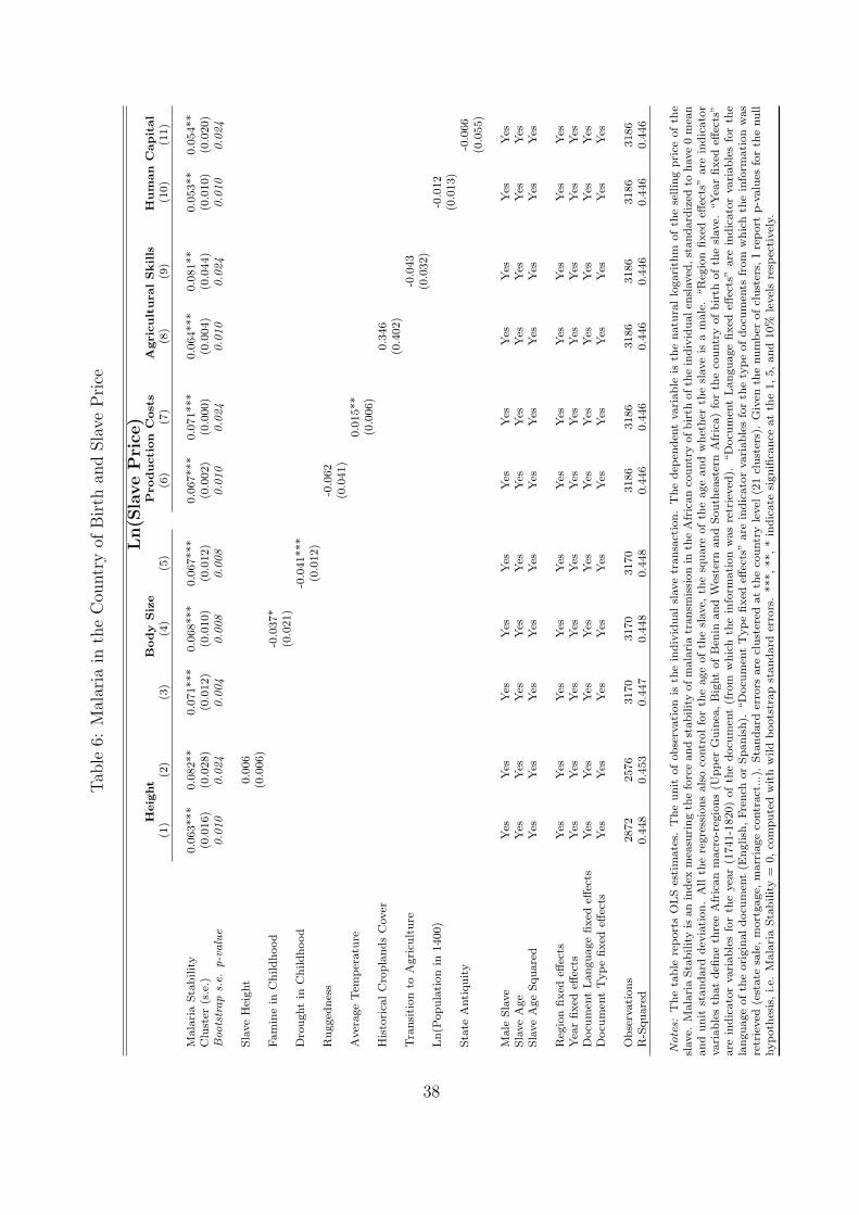
Tab

le6:

Mal

aria

inth

eC

ountr

yof

Bir

than

dSla

veP

rice

Ln(S

lavePrice

)H

eig

ht

Bod

yS

ize

Prod

ucti

on

Cost

sA

gric

ult

ural

Skil

lsH

um

an

Cap

ital

(1)

(2)

(3)

(4)

(5)

(6)

(7)

(8)

(9)

(10)

(11)

Mala

ria

Sta

bilit

y0.0

63***

0.0

82**

0.0

71***

0.0

68***

0.0

67***

0.0

67***

0.0

71***

0.0

64***

0.0

81**

0.0

53**

0.0

54**

Clu

ster

(s.e

.)(0

.016)

(0.0

28)

(0.0

12)

(0.0

10)

(0.0

12)

(0.0

02)

(0.0

00)

(0.0

04)

(0.0

44)

(0.0

10)

(0.0

20)

Boo

tstraps.e.

p-value

0.010

0.024

0.004

0.008

0.008

0.010

0.024

0.010

0.024

0.010

0.024

Sla

ve

Hei

ght

0.0

06

(0.0

06)

Fam

ine

inC

hild

hood

-0.0

37*

(0.0

21)

Dro

ught

inC

hild

hood

-0.0

41***

(0.0

12)

Ru

gged

nes

s-0

.062

(0.0

41)

Aver

age

Tem

per

atu

re0.0

15**

(0.0

06)

His

tori

cal

Cro

pla

nd

sC

over

0.3

46

(0.4

02)

Tra

nsi

tion

toA

gri

cult

ure

-0.0

43

(0.0

32)

Ln

(Pop

ula

tion

in1400)

-0.0

12

(0.0

13)

Sta

teA

nti

qu

ity

-0.0

66

(0.0

55)

Male

Sla

ve

Yes

Yes

Yes

Yes

Yes

Yes

Yes

Yes

Yes

Yes

Yes

Sla

ve

Age

Yes

Yes

Yes

Yes

Yes

Yes

Yes

Yes

Yes

Yes

Yes

Sla

ve

Age

Squ

are

dY

esY

esY

esY

esY

esY

esY

esY

esY

esY

esY

es

Reg

ion

fixed

effec

tsY

esY

esY

esY

esY

esY

esY

esY

esY

esY

esY

esY

ear

fixed

effec

tsY

esY

esY

esY

esY

esY

esY

esY

esY

esY

esY

esD

ocu

men

tL

an

gu

age

fixed

effec

tsY

esY

esY

esY

esY

esY

esY

esY

esY

esY

esY

esD

ocu

men

tT

yp

efi

xed

effec

tsY

esY

esY

esY

esY

esY

esY

esY

esY

esY

esY

es

Ob

serv

ati

on

s2872

2576

3170

3170

3170

3186

3186

3186

3186

3186

3186

R-S

qu

are

d0.4

48

0.4

53

0.4

47

0.4

48

0.4

48

0.4

46

0.4

46

0.4

46

0.4

46

0.4

46

0.4

46

Notes:

Th

eta

ble

rep

ort

sO

LS

esti

mate

s.T

he

un

itof

ob

serv

ati

on

isth

ein

div

idu

al

slave

tran

sact

ion

.T

he

dep

end

ent

vari

ab

leis

the

natu

ral

logari

thm

of

the

sellin

gp

rice

of

the

slave.

Mala

ria

Sta

bilit

yis

an

index

mea

suri

ng

the

forc

ean

dst

ab

ilit

yof

mala

ria

tran

smis

sion

inth

eA

fric

an

cou

ntr

yof

bir

thof

the

ind

ivid

ual

ensl

aved

,st

an

dard

ized

toh

ave

0m

ean

an

du

nit

stan

dard

dev

iati

on

.A

llth

ere

gre

ssio

ns

als

oco

ntr

ol

for

the

age

of

the

slave,

the

squ

are

of

the

age

an

dw

het

her

the

slave

isa

male

.“R

egio

nfi

xed

effec

ts”

are

ind

icato

rvari

ab

les

that

defi

ne

thre

eA

fric

an

macr

o-r

egio

ns

(Up

per

Gu

inea

,B

ight

of

Ben

inan

dW

este

rnan

dS

ou

thea

ster

nA

fric

a)

for

the

cou

ntr

yof

bir

thof

the

slave.

“Y

ear

fixed

effec

ts”

are

ind

icato

rvari

ab

les

for

the

yea

r(1

741-1

820)

of

the

docu

men

t(f

rom

wh

ich

the

info

rmati

on

was

retr

ieved

).“D

ocu

men

tL

an

gu

age

fixed

effec

ts”

are

ind

icato

rvari

ab

les

for

the

lan

gu

age

of

the

ori

gin

al

docu

men

t(E

nglish

,F

ren

chor

Sp

an

ish

).“D

ocu

men

tT

yp

efi

xed

effec

ts”

are

ind

icato

rvari

ab

les

for

the

typ

eof

docu

men

tsfr

om

wh

ich

the

info

rmati

on

was

retr

ieved

(est

ate

sale

,m

ort

gage,

marr

iage

contr

act

...)

.S

tan

dard

erro

rsare

clu

ster

edat

the

countr

yle

vel

(21

clu

ster

s).

Giv

enth

enu

mb

erof

clu

ster

s,I

rep

ort

p-v

alu

esfo

rth

enull

hyp

oth

esis

,i.e.

Mala

ria

Sta

bilit

y=

0,

com

pu

ted

wit

hw

ild

boots

trap

stan

dard

erro

rs.

***,

**,

*in

dic

ate

sign

ifica

nce

at

the

1,

5,

an

d10%

level

sre

spec

tivel

y.

38

References

Acemoglu, D., C. Garcıa-Jimeno, and J. Robinson (2012): “Finding Eldorado: Slavery

and Long-run Development in Colombia,” Journal of Comparative Economics.

Acemoglu, D., and S. Johnson (2006): “Disease and development: the effect of life ex-

pectancy on economic growth,” .

Acemoglu, D., S. Johnson, and J. A. Robinson (2001): “The Colonial Origins of Compar-

ative Development: An Empirical Investigation,” American Economic Review, 91(5), 1369–

1401.

Alesina, A., P. Giuliano, and N. Nunn (2013): “On the origins of gender roles: Women

and the plough,” The Quarterly Journal of Economics, 128(2), 469–530.

Allison, A. (2006): “Genetic factors in resistance to malaria,” Annals of the New York

Academy of Sciences, 91(3), 710–729.

Alsan, M. (2015): “The Effect of the TseTse Fly on African Development,” American Eco-

nomic Review, 105(1), 382–410.

Ashraf, Q., and O. Galor (2013): “The out of Africa hypothesis, human genetic diversity,

and comparative economic development,” The American Economic Review, 103(1), 1–46.

Berlin, I. (2009): Many thousands gone: The first two centuries of slavery in North America.

Harvard University Press.

Bertocchi, G., and A. Dimico (2014): “Slavery, education, and inequality,” European

Economic Review, 70, 197–209.

Bleakley, H. (2007): “Disease and development: evidence from hookworm eradication in the

American South,” The Quarterly Journal of Economics, 122(1), 73.

(2010): “Malaria Eradication in the Americas: A Retrospective Analysis of Childhood

Exposure,” American Economic Journal: Applied Economics, 2(2), 1–45.

Bobonis, G. J., and P. M. Morrow (2014): “Labor coercion and the accumulation of

human capital,” Journal of Development Economics, 108, 32–53.

Bruhn, M., and F. Gallego (2012): “Good, bad, and ugly colonial activities: do they

matter for economic development?,” Review of Economics and Statistics, 94(2), 433–461.

39

Carter, R., and K. N. Mendis (2002): “Evolutionary and historical aspects of the burden

of malaria,” Clinical microbiology reviews, 15(4), 564–594.

Cervellati, M., and U. Sunde (2011): “Disease and development: The role of life ex-

pectancy reconsidered,” Economics Letters, 113(3), 269–272.

Childs, S. J. R. (1940): “Malaria and colonization in the Carolina low country, 1526-1696,”

Ph.D. thesis, Johns Hopkins Press.

Coelho, P., and R. McGuire (1997): “African and European Bound Labor in the British

New World: The Biological Consequences of Economic Choices,” The Journal of economic

history, 57(01), 83–115.

Coelho, P. R., and R. A. McGuire (2006): “Racial differences in disease susceptibilities:

Intestinal worm infections in the early twentieth-century American South,” Social history of

medicine, 19(3), 461–482.

Conley, T. G. (1999): “GMM estimation with cross sectional dependence,” Journal of econo-

metrics, 92(1), 1–45.

Curtin, P. (1968): “Epidemiology and the slave trade,” Political Science Quarterly, pp. 190–

216.

Curtin, P. D. (1993): “Disease exchange across the tropical Atlantic,” History and philosophy

of the life sciences, pp. 329–356.

Dell, M. (2010): “The persistent effects of Peru’s mining Mita,” Econometrica, 78(6), 1863–

1903.

Dell, M. (2012): “Path dependence in development: Evidence from the Mexican Revolution,”

Unpublished manuscript, Department of Economics, Harvard University.

Depetris-Chauvin, E., and D. N. Weil (2013): “Malaria and Early African Develop-

ment: Evidence from the Sickle Cell Trait,” Discussion paper, National Bureau of Economic

Research.

Diamond, J., and L. Ford (2000): “Guns, germs, and steel: the fates of human societies,”

Perspectives in Biology and Medicine, 43(4), 609.

Dobson, M. (1989): “History of malaria in England.,” Journal of the Royal Society of

Medicine, 82(Suppl 17), 3.

40

Doolan, D. L., C. Dobano, and J. K. Baird (2009): “Acquired immunity to malaria,”

Clinical microbiology reviews, 22(1), 13–36.

Engerman, S., and K. Sokoloff (1997): Factor Endowments, Institutions, and Differential

Growth Paths among New World Economies, vol. 89. Stanford University Press.

Fenske, J., and N. Kala (2015): “Climate and the slave trade,” Journal of Development

Economics, 112, 19–32.

Fogel, R. W. (1994): Without consent or contract: the rise and fall of American slavery.

WW Norton & Company.

Fogel, R. W., and L. Engerman, S (1974): “Time on the Cross,” The Economics of

American Negro Slavery, 2, 242–243.

Galenson, D. W. (1981): White servitude in colonial America: An economic analysis. Cam-

bridge University Press Cambridge.

Gallup, J. L., J. D. Sachs, and A. D. Mellinger (1999): “Geography and economic

development,” International regional science review, 22(2), 179–232.

Geggus, D. (2001): “The French slave trade: an overview,” The William and Mary Quarterly,

pp. 119–138.

Gething, P. W., T. P. Van Boeckel, D. L. Smith, C. A. Guerra, A. P. Patil,

R. W. Snow, and S. I. Hay (2011): “Modelling the global constraints of temperature on

transmission of Plasmodium falciparum and P. vivax,” Parasit Vectors, 4(92), 4.

Goldin, C., and K. L. Sokoloff (1981): “The Relative Productivity Hypothesis of Indus-

trialization: The American Case, 1820-1850,” .

Goldin, C. D. (1976): Urban slavery in the American South, 1820-1860: a quantitative

history. University of Chicago Press.

Hall, G. M. (2005): Slavery and African ethnicities in the Americas: restoring the links.

University of North Carolina Press.

Hanes, C. (1996): “Turnover cost and the distribution of slave labor in Anglo-America,” The

Journal of Economic History, 56(02), 307–329.

41

Hay S.I., Guerra C.A., T. A. N. A. . S. R. (2004): “The global distribution and population

at risk of malaria: past, present and future,” Lancet Infectious Diseases, 4(6), 327–336.

Hedrick, P. (2011): “Population genetics of malaria resistance in humans,” Heredity, 107(4),

283–304.

Hong, S. C. (2007): “The burden of early exposure to malaria in the united states, 1850–1860:

Malnutrition and immune disorders,” The journal of economic history, 67(04), 1001–1035.

Humphreys, M. (2001): Malaria: poverty, race, and public health in the United States. JHU

Press.

Kiple, K., and V. King (2003): Another Dimension to the Black Diaspora: diet, disease and

racism. Cambridge University Press.

Kiszewski, A., A. Mellinger, A. Spielman, P. Malaney, S. E. Sachs, and J. Sachs

(2004): “A global index representing the stability of malaria transmission,” The American

journal of tropical medicine and hygiene, 70(5), 486–498.

Kotlikoff, L. J. (1979): “The structure of slave prices in New Orleans, 1804 to 1862,”

Economic Inquiry, 17(4), 496–518.

Kwiatkowski, D. P. (2005): “How malaria has affected the human genome and what human

genetics can teach us about malaria,” The American Journal of Human Genetics, 77(2),

171–192.

Littlefield, D. C. (1981): “Rice and slaves,” Ethnicity and the Slave Trade in Colonial

South Carolina.

Lysenko, A.J., S. I. (1968): “Geography of malaria. A medico-geographic profile of an ancient

disease,” Medicinskaja Geografija, p. 25146.

Mackinnon, M. J., T. W. Mwangi, R. W. Snow, K. Marsh, and T. N. Williams

(2005): “Heritability of malaria in Africa,” PLoS medicine, 2(12), e340.

Mallard, R. Q. (1892): Plantation life before emancipation. Negro History Press.

Mann, C. C. (2011): 1493: Uncovering the New World Columbus Created. Alfred a Knopf

Incorporated.

42

Mauro, F. (1964): L’expansion europeenne:(1600-1870), no. 27. Presses universitaires de

France.

McNeill, J. (2010): “Mosquito Empires: Ecology And War In The Greater Caribbean, 1620-

1914,” .

Menard, R. R. (2001): Migrants, Servants and Slaves: Unfree Labor in Colonial British

America, vol. 699. Variorum.

Michalopoulos, S. (2012): “The origins of ethnolinguistic diversity,” The American eco-

nomic review, 102(4), 1508.

Nunn, N. (2007): “The long-term effects of Africa’s slave trades,” .

Nunn, N. (2008): “The Long-Term Effects of Africa’s Slave Trades,” The Quarterly Journal

of Economics, 123(1), 139–176.

Nunn, N., and D. Puga (2012): “Ruggedness: The blessing of bad geography in Africa,”

Review of Economics and Statistics, 94(1), 20–36.

Nunn, N., and L. Wantchekon (2011): “The Slave Trade and the Origins of Mistrust in

Africa,” The American Economic Review, 101(7), 3221–3252.

Oscar, and M. F. Handlin (1950): “Origins of the Southern labor system,” The William

and Mary Quarterly: A Magazine of Early American History, pp. 199–222.

Oster, E. (2013): “Unobservable selection and coefficient stability: Theory and validation,”

Discussion paper, National Bureau of Economic Research.

Packard, R. M. (2007): The making of a tropical disease: a short history of malaria. Johns

Hopkins University Press, Baltimore.

Rutman, D. B., and A. H. Rutman (1976): “Of agues and fevers: malaria in the early

Chesapeake.,” The William and Mary Quarterly, 33, 31.

Savitt, T. L. (2002): Medicine and slavery: The diseases and health care of blacks in ante-

bellum Virginia. University of Illinois Press.

Sheridan, R. B. (1981): “The Guinea Surgeons on the Middle Passage: The Provision of

Medical Services in the British Slave Trade,” International Journal of African Historical

Studies, pp. 601–625.

43

Sokoloff, K., and S. Engerman (2000): “History lessons: Institutions, factors endow-

ments, and paths of development in the new world,” The Journal of Economic Perspectives,

14(3), 217–232.

Stampp, K. M. (2011): The peculiar institution. Alfred A. Knopf.

Stevenson, M. M., and E. M. Riley (2004): “Innate immunity to malaria,” Nature Reviews

Immunology, 4(3), 169–180.

Van Dine, D. (1916): “The relation of malaria to crop production,” Scientific Monthly Novem-

ber, pp. 431–439.

Voigtlander, N., and H.-J. Voth (2012): “The Three Horsemen of Riches: Plague, War,

and Urbanization in Early Modern Europe,” The Review of Economic Studies, p. rds034.

Waring, J. I. (1975): “Colonial medicine in Georgia and South Carolina.,” The Georgia

historical quarterly, 59, 141.

Wax, D. D. (1973): “Preferences for slaves in colonial America,” Journal of Negro History,

pp. 371–401.

Weil, D. N. (2007): “Accounting for The Effect of Health on Economic Growth,” The Quar-

terly Journal of Economics, 122(3), 1265–1306.

Whatley, W., and R. Gillezeau (2011): “The impact of the transatlantic slave trade on

ethnic stratification in Africa,” The American Economic Review, pp. 571–576.

Wiecek, W. M. (1977): “The statutory law of slavery and race in the thirteen mainland

colonies of British America,” The William and Mary Quarterly: A Magazine of Early Amer-

ican History, pp. 258–280.

Wolfe, N. D., C. P. Dunavan, and J. Diamond (2007): “Origins of major human infec-

tious diseases,” Nature, 447(7142), 279–283.

Wood, P. (1974): “Black Majority: Negroes in Colonial South Carolina from 1670 through

the Stono Rebellion,” Norton Library, New York.

Wright, G. (2003): “Slavery and American agricultural history,” Agricultural history, pp.

527–552.

44

Yalcindag, E., E. Elguero, C. Arnathau, P. Durand, J. Akiana, T. J. Ander-

son, A. Aubouy, F. Balloux, P. Besnard, H. Bogreau, et al. (2012): “Multiple

independent introductions of Plasmodium falciparum in South America,” Proceedings of the

National Academy of Sciences, 109(2), 511–516.

45

SIDE EFFECTS OF IMMUNITIES: THE AFRICAN SLAVE TRADE

ONLINE APPENDIX

APPENDIX A: DATA SOURCES AND ADDITIONAL TABLES

Appendix A.1: Malaria and African Slavery - 1790 United States Counties

Data Sources: 1790 United States CountyShare of SlavesRatio of slaves to total population in the county in 1790. Source: Historical U.S. census. www.nhgis.org.Share of BlacksRatio of blacks to total population in the county in 1790. Source: Historical U.S. census. www.nhgis.org.Malaria StabilityAverage Malaria Stability Index in the state. Source: average Malaria Stability is constructed as thestate average of the Malaria Stability index from Kiszewski et al. (2004).Malaria EndemicityAverage Historical Malaria Endemicity in the state. Source: average Historical Malaria Endemicityis constructed as the state average of the Malaria Endemicity level, devised by Lysenko (1968) anddigitalized by Hay (2004).Crop Suitability IndexesEstimated suitability index (value) for cultivating cotton, coffee, rice, sugar, tea and tobacco with Lowinput in a rainfed agriculture. Source: FAO/IIASA, 2011. Global Agro-ecological Zones (GAEZv3.0).FAO Rome, Italy and IIASA, Laxenburg, Austria. http://gaez.fao.org/Main.html.Distance to SeaAverage county distance to seas and oceans (1000 km). Source: GSHHG - A Global Self-consistent,Hierarchical, High-resolution Geography Database, computed using ArcGIS with data in North AmericaEquidistant Conic projection.Distance to RiversAverage county distance to inland water bodies, rivers and lakes (1000 km). Source: computed usingArcGIS with data in North America Equidistant Conic projection.Distance to CharlestonAverage county distance to to Charleston country (1000 km). Source: computed using ArcGIS with datain North America Equidistant Conic projection.Average PrecipitationAverage county monthly precipitation mm/month (baseline period 1961-1990). Source: CRU CL 2.0data from New (2002).Average TemperatureMean annual county temperature (baseline period 1961-1990). Source: from FAO/IIASA, 2011-2012.Global Agro-ecological Zones (GAEZ v3.0). FAO Rome, Italy and IIASA, Laxenburg, Austria.Total PopulationTotal population in the county in 1790. Source: Historical U.S. census. www.nhgis.org.Share of Families with SlavesShare of families owning slaves in the county in 1790. Source: Historical U.S. census. www.nhgis.org.BlacksBlack People in the county in 1790. Source: Historical U.S. census. www.nhgis.org.

46

Table 8: Summary Statistics of Cross-County Analysis

Variable Mean Std. Dev. Min Max NShare of Slaves 0.224 0.205 0 0.762 285Share of Blacks 0.239 0.209 0.002 0.772 285Malaria Stability 0 1 -1.493 2.24 285Malaria Endemicity 0 1 -2.107 0.97 285Cotton Suitability 2469.092 1746.858 0 7486.781 285Rice Suitability 1071.552 1422.706 0 5802.241 285Sugar Suitability 140.035 508.068 0 2874.037 285Tea Suitability 2142.92 2162.941 0 7170.96 285Tobacco Suitability 4000.996 1380.764 0.305 7261.313 285Distance Sea 0.118 0.136 0 0.713 285Distance River 0.011 0.006 0.001 0.035 285Distance Charleston 0.63 0.363 0.001 1.689 285Average Precipitation 95.261 8.106 71.054 119.591 285Average Temperature 12.588 3.225 4.625 19.337 285Total Population 13662.926 11349.489 305 75980 285Share of Families with Slaves 0.234 0.183 0 0.684 142Blacks 2643.519 3886.554 16 51583 285

47

Tab

le9:

Cro

ss-c

orre

lati

onta

ble

Vari

ab

les

(1)

(2)

(3)

(4)

(5)

(6)

(7)

(8)

(9)

(10)

(11)

(12)

(13)

(14)

(15)

(16)

(17)

(1)

Sh

are

of

Sla

ves

1.0

00

(2)

Sh

are

of

Bla

cks

0.9

97

1.0

00

(3)

Mala

ria

Sta

bilit

y0.6

05

0.5

91

1.0

00

(4)

His

tori

cal

Mala

ria

En

dem

icit

y0.7

00

0.6

87

0.7

80

1.0

00

(5)

Cott

on

Su

itab

ilit

y0.4

37

0.4

27

0.7

12

0.5

62

1.0

00

(6)

Ric

eS

uit

ab

ilit

y0.0

46

0.0

37

0.4

79

0.2

08

0.3

82

1.0

00

(7)

Su

gar

Su

itab

ilit

y0.2

95

0.2

84

0.4

07

0.2

62

0.1

11

0.3

56

1.0

00

(8)

Tea

Su

itab

ilit

y0.5

25

0.5

14

0.6

62

0.6

37

0.5

02

0.2

64

0.1

04

1.0

00

(9)

Tob

acc

oS

uit

ab

ilit

y-0

.042

-0.0

50

0.2

12

0.0

92

0.5

49

0.1

82

-0.1

30

0.1

82

1.0

00

(10)

Sea

Dis

tan

ce-0

.273

-0.3

03

0.0

84

-0.1

43

0.1

73

0.2

04

-0.1

04

0.0

59

0.2

84

1.0

00

(11)

Riv

erD

ista

nce

-0.1

96

-0.2

05

-0.0

31

-0.1

05

0.0

16

-0.1

29

-0.0

76

-0.0

55

0.1

01

0.0

94

1.0

00

(12)

Dis

tan

ceto

Ch

arl

esto

n-0

.552

-0.5

35

-0.8

86

-0.7

46

-0.6

57

-0.3

93

-0.3

76

-0.6

96

-0.3

15

-0.2

10

0.0

67

1.0

00

(13)

Aver

age

Pre

cip

itati

on

-0.0

39

-0.0

40

0.3

18

0.0

64

0.0

28

0.5

35

0.3

42

0.2

33

-0.0

63

-0.0

82

0.0

23

-0.2

87

1.0

00

(14)

Aver

age

Tem

per

atu

re0.6

30

0.6

23

0.9

20

0.7

50

0.6

88

0.5

14

0.4

57

0.6

70

0.2

68

0.0

33

-0.1

59

-0.9

35

0.3

63

1.0

00

(15)

Tota

lP

op

ula

tion

-0.2

69

-0.2

61

-0.3

82

-0.3

27

-0.2

93

-0.2

14

-0.0

87

-0.3

82

-0.0

25

-0.2

19

0.1

51

0.4

64

0.0

00

-0.4

27

1.0

00

(16)

Sh

are

of

Fam

ilie

sw

ith

Sla

ves

0.9

51

0.9

54

0.6

41

0.6

20

0.4

90

0.3

11

0.3

30

0.4

10

-0.1

16

-0.2

95

-0.3

08

-0.5

56

0.1

87

0.6

66

-0.2

77

1.0

00

(17)

Bla

cks

0.6

15

0.6

17

0.3

21

0.3

65

0.2

29

-0.0

49

0.2

33

0.2

18

-0.0

14

-0.2

18

-0.0

48

-0.2

83

-0.0

62

0.3

15

0.2

51

0.5

26

1.0

00

48

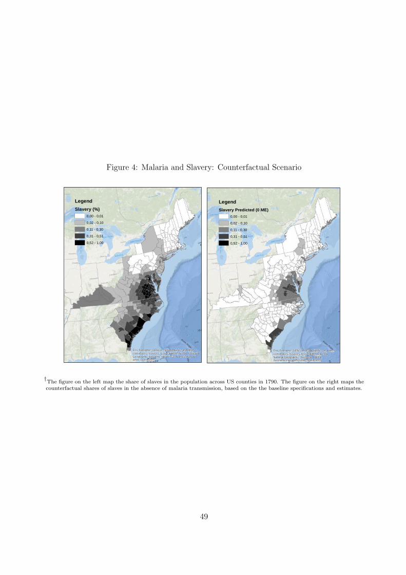
Figure 4: Malaria and Slavery: Counterfactual Scenario

Esri, DeLorme, GEBCO, NOAA NGDC, and othercontributors; Sources: Esri, GEBCO, NOAA,National Geographic, DeLorme, HERE,Geonames.org, and other contributors

Esri, DeLorme, GEBCO, NOAA NGDC, and othercontributors; Sources: Esri, GEBCO, NOAA, NationalGeographic, DeLorme, HERE, Geonames.org, andother contributors

Legend

Slavery Predicted (0 ME)

0,00 - 0,01

0,02 - 0,10

0,11 - 0,30

0,31 - 0,51

0,52 - 1,00

Legend

Slavery (%)0,00 - 0,01

0,02 - 0,10

0,11 - 0,30

0,31 - 0,51

0,52 - 1,00

†The figure on the left map the share of slaves in the population across US counties in 1790. The figure on the right maps thecounterfactual shares of slaves in the absence of malaria transmission, based on the the baseline specifications and estimates.

49

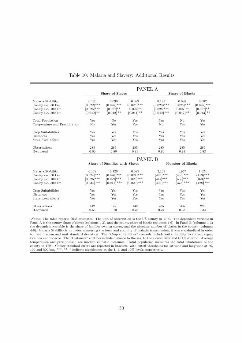
Table 10: Malaria and Slavery: Additional Results

PANEL AShare of Slaves Share of Blacks

Malaria Stability 0.120 0.090 0.089 0.123 0.088 0.087Conley s.e. 50 km (0.022)*** (0.025)*** (0.025)*** (0.023)*** (0.025)*** (0.025)***Conley s.e. 100 km [0.025]*** [0.027]** [0.027]** [0.026]*** [0.027]** [0.027]**Conley s.e. 500 km {0.040}** {0.042}** {0.044}** {0.040}*** {0.042}** {0.043}**

Total Population Yes No Yes Yes No YesTemperature and Precipitation No Yes Yes No Yes Yes

Crop Suitabilities Yes Yes Yes Yes Yes YesDistances Yes Yes Yes Yes Yes YesState fixed effects Yes Yes Yes Yes Yes Yes

Observations 285 285 285 285 285 285R-squared 0.60 0.80 0.81 0.80 0.81 0.82

PANEL BShare of Families with Slaves Number of Blacks

Malaria Stability 0.129 0.126 0.085 2,109 1,957 1,624Conley s.e. 50 km (0.024)*** (0.026)*** (0.024)*** (405)*** (485)*** (419)***Conley s.e. 100 km [0.026]*** [0.029]*** [0.028]*** [447]*** [535]*** [463]***Conley s.e. 500 km {0.034}*** {0.041}*** {0.029}*** {409}*** {375}*** {428}***

Crop Suitabilities Yes Yes Yes Yes Yes YesDistances Yes Yes Yes Yes Yes YesState fixed effects Yes Yes Yes Yes Yes Yes

Observations 142 142 142 285 285 285R-squared 0.65 0.70 0.78 0.24 0.33 0.34

Notes: The table reports OLS estimates. The unit of observation is the US county in 1790. The dependent variable inPanel A is the county share of slaves (columns 1-3), and the county share of blacks (columns 4-6). In Panel B (columns 1-3)the dependent variable is the share of families owning slaves, and the absolute number of blacks in the county (columns4-6). Malaria Stability is an index measuring the force and stability of malaria transmission, it was standardized in orderto have 0 mean and unit standard deviation. The “Crop suitabilities” controls include soil suitability to cotton, sugar,rice, tea and tobacco. The “Distances” controls include distance to the sea, to the closest river and to Charleston. Averagetemperature and precipitation are modern climatic measures. Total population measures the total inhabitants of thecounty in 1790. Conley standard errors are reported in brackets, with cutoff thresholds for latitude and longitude at 50,100 and 500 km. ***, **, * indicate significance at the 1, 5, and 10% levels respectively.

50

Tab

le11

:M

alar

iaan

dSla

very

acro

ssU

SC

ounti

es

DependentVariable:Share

ofSlaves1790

PA

NE

LA

Mala

ria

Sta

bilit

y-

Fu

llS

am

ple

Mala

ria

Sta

bilit

y0.1

24

0.1

64

0.1

97

0.1

57

0.1

66

0.1

53

0.1

70

0.1

44

Con

ley

s.e.

50

km

(0.0

10)*

**

(0.0

24)*

**

(0.0

27)*

**

(0.0

23)*

**

(0.0

24)*

**

(0.0

22)*

**

(0.0

23)*

**

(0.0

24)*

**

Con

ley

s.e.

100

km

[0.0

16]*

**

[0.0

29]*

**

[0.0

33]*

**

[0.0

29]*

**

[0.0

30]*

**

[0.0

27]*

**

[0.0

29]*

**

[0.0

28]*

**

Con

ley

s.e.

500

km

{0.0

30}*

**{0

.046}*

**{0

.049}*

**{0

.048}*

**

{0.0

47}*

**{0

.036}*

**

{0.0

46}*

**{0

.037}*

**

CropSuitability

Indexes

Cott

on

Su

itab

ilit

yN

oN

oY

esN

oN

oN

oN

oY

esS

ugar

Su

itab

ilit

yN

oN

oN

oY

esN

oN

oN

oY

esR

ice

Su

itab

ilit

yN

oN

oN

oN

oY

esN

oN

oY

esT

eaS

uit

ab

ilit

yN

oN

oN

oN

oN

oY

esN

oY

esT

ob

acc

oS

uit

ab

ilit

yN

oN

oN

oN

oN

oN

oY

esY

es

Sta

teF

EN

oY

esY

esY

esY

esY

esY

esY

es

Ob

serv

ati

on

s285

285

285

285

285

285

285

285

R-s

qu

are

d0.3

66

0.6

01

0.6

21

0.6

48

0.6

09

0.6

15

0.6

58

0.7

16

PA

NE

LB

PA

NE

LC

PA

NE

LD

Mala

ria

Sta

bilit

yM

ala

ria

En

dem

icit

yM

ala

ria

Sta

bilit

yF

ull

Sam

ple

Fu

llS

am

ple

On

lyS

lave

Sta

tes

Mala

ria

Sta

bilit

y0.1

06

0.1

53

0.1

51

0.1

21

0.1

65

0.1

20

Con

ley

s.e.

50

km

(0.0

20)*

**

(0.0

22)*

**

(0.0

28)*

**

(0.0

22)*

**

(0.0

24)*

**

(0.0

23)*

**

Con

ley

s.e.

100

km

[0.0

23]*

**

[0.0

25]*

**

[0.0

33]*

**

[0.0

25]*

**

[0.0

30]*

**

[0.0

26]*

**

Con

ley

s.e.

500

km

{0.0

36}*

**{0

.034}*

**{0

.046}*

**{0

.040}*

**

{0.0

41}*

**{0

.046}*

**

Mala

ria

En

dem

icit

y0.1

23

0.0

48

Con

ley

s.e.

50

km

(0.0

16)*

**

(0.0

14)*

**

Con

ley

s.e.

100

km

[0.0

22]*

**

[0.0

17]*

**

Con

ley

s.e.

500

km

{0.0

20}*

**{0

.010}*

**

CropSuitability

Indexes

Yes

Yes

Yes

Yes

No

Yes

No

Yes

Distances

Sea

Dis

tan

ceY

esN

oN

oY

esN

oY

esN

oY

esR

iver

Dis

tan

ceN

oY

esN

oY

esN

oY

esN

oY

esD

ista

nce

Ch

arl

esto

nN

oN

oY

esY

esN

oY

esN

oY

es

Sta

teF

EY

esY

esY

esY

esY

esY

esY

esY

es

Ob

serv

ati

on

s285

285

285

285

285

285

244

244

R-s

qu

are

d0.7

90.7

30.7

20.7

90.6

20.7

70.5

10.7

5

Notes:

Th

eta

ble

rep

ort

sO

LS

esti

mate

s.T

he

un

itof

ob

serv

ati

on

isth

eU

Sco

unty

in1790.

Th

ed

epen

den

tvari

ab

leis

the

share

of

slaves

inth

eco

unty

pop

ula

tion

.In

pan

elA

,B

an

dD

,th

eex

pla

nato

ryvari

ab

leis

Mala

ria

Sta

bilit

y,an

ind

exm

easu

rin

gth

efo

rce

an

dst

ab

ilit

yof

mala

ria

tran

smis

sion

,st

an

dard

ized

inord

erto

have

0m

ean

an

du

nit

stan

dard

dev

iati

on

.In

Pan

elC

the

exp

lan

ato

ryvari

ab

leis

Mala

ria

En

dem

icit

y,an

ind

exm

easu

rin

gth

em

ala

ria

para

siti

zati

on

rate

at

the

beg

inn

ing

of

the

20th

centu

ry,

stan

dard

ized

inord

erto

have

0m

ean

an

du

nit

stan

dard

dev

iati

on

.F

or

the

sam

ple

of

“sl

ave

state

s”,

Iex

clu

de

cou

nti

esin

Con

nec

ticu

t,M

ass

ach

use

tts,

New

Ham

psh

ire,

Rh

ode

Isla

nd

an

dV

erm

ont.

Con

ley

stan

dard

erro

rsare

rep

ort

edin

bra

cket

s,w

ith

cuto

ffth

resh

old

sfo

rla

titu

de

an

dlo

ngit

ud

eat

50,

100

an

d500

km

.***,

**,

*in

dic

ate

sign

ifica

nce

at

the

1,

5,

an

d10%

level

sre

spec

tivel

y.

51

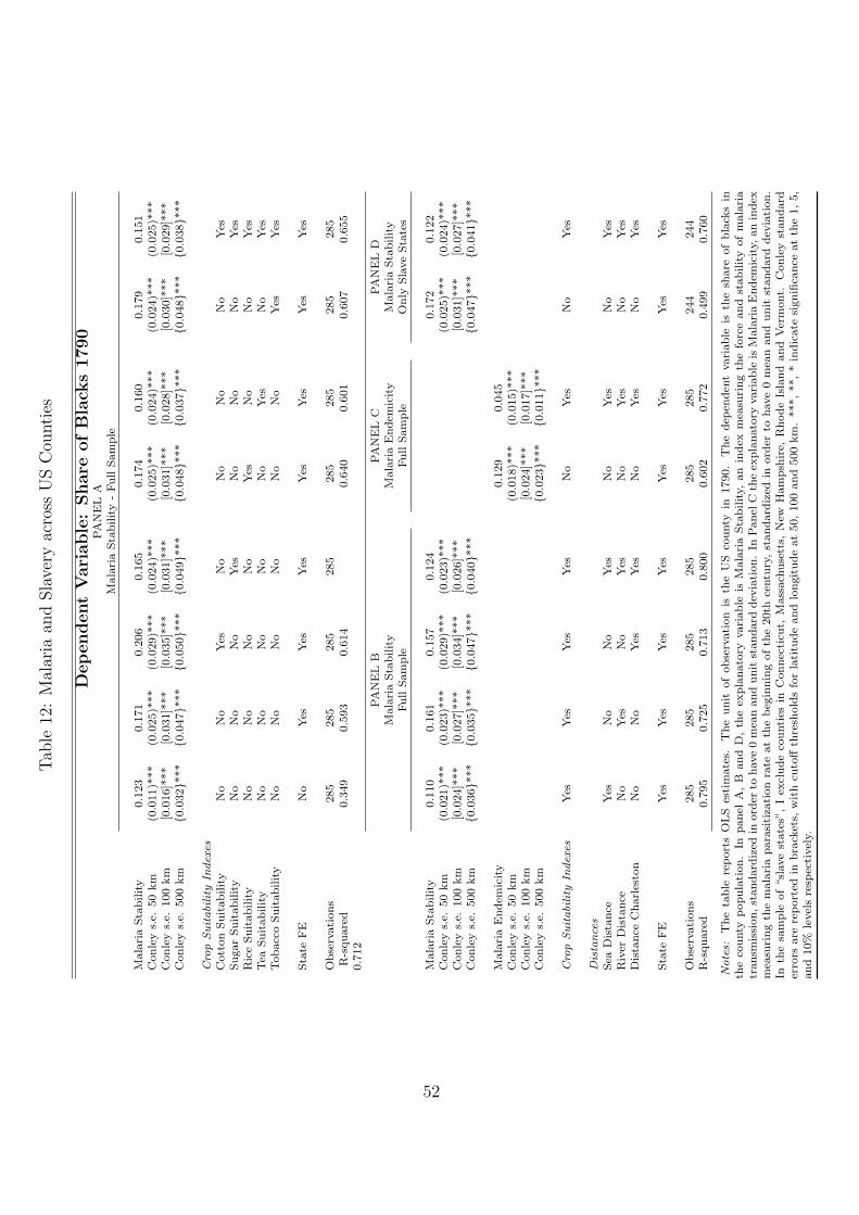
Tab

le12

:M

alar

iaan

dSla

very

acro

ssU

SC

ounti

es

DependentVariable:Share

ofBlack

s1790

PA

NE

LA

Mala

ria

Sta

bilit

y-

Fu

llS

am

ple

Mala

ria

Sta

bilit

y0.1

23

0.1

71

0.2

06

0.1

65

0.1

74

0.1

60

0.1

79

0.1

51

Con

ley

s.e.

50

km

(0.0

11)*

**

(0.0

25)*

**

(0.0

29)*

**

(0.0

24)*

**

(0.0

25)*

**

(0.0

24)*

**

(0.0

24)*

**

(0.0

25)*

**

Con

ley

s.e.

100

km

[0.0

16]*

**

[0.0

31]*

**

[0.0

35]*

**

[0.0

31]*

**

[0.0

31]*

**

[0.0

28]*

**

[0.0

30]*

**

[0.0

29]*

**

Con

ley

s.e.

500

km

{0.0

32}*

**{0

.047}*

**{0

.050}*

**{0

.049}*

**

{0.0

48}*

**{0

.037}*

**

{0.0

48}*

**{0

.038}*

**

CropSuitability

Indexes

Cott

on

Su

itab

ilit

yN

oN

oY

esN

oN

oN

oN

oY

esS

ugar

Su

itab

ilit

yN

oN

oN

oY

esN

oN

oN

oY

esR

ice

Su

itab

ilit

yN

oN

oN

oN

oY

esN

oN

oY

esT

eaS

uit

ab

ilit

yN

oN

oN

oN

oN

oY

esN

oY

esT

ob

acc

oS

uit

ab

ilit

yN

oN

oN

oN

oN

oN

oY

esY

es

Sta

teF

EN

oY

esY

esY

esY

esY

esY

esY

es

Ob

serv

ati

on

s285

285

285

285

285

285

285

285

R-s

qu

are

d0.3

49

0.5

93

0.6

14

0.6

40

0.6

01

0.6

07

0.6

55

0.7

12

PA

NE

LB

PA

NE

LC

PA

NE

LD

Mala

ria

Sta

bilit

yM

ala

ria

En

dem

icit

yM

ala

ria

Sta

bilit

yF

ull

Sam

ple

Fu

llS

am

ple

On

lyS

lave

Sta

tes

Mala

ria

Sta

bilit

y0.1

10

0.1

61

0.1

57

0.1

24

0.1

72

0.1

22

Con

ley

s.e.

50

km

(0.0

21)*

**

(0.0

23)*

**

(0.0

29)*

**

(0.0

23)*

**

(0.0

25)*

**

(0.0

24)*

**

Con

ley

s.e.

100

km

[0.0

24]*

**

[0.0

27]*

**

[0.0

34]*

**

[0.0

26]*

**

[0.0

31]*

**

[0.0

27]*

**

Con

ley

s.e.

500

km

{0.0

36}*

**{0

.035}*

**{0

.047}*

**{0

.040}*

**

{0.0

47}*

**{0

.041}*

**

Mala

ria

En

dem

icit

y0.1

29

0.0

45

Con

ley

s.e.

50

km

(0.0

18)*

**

(0.0

15)*

**

Con

ley

s.e.

100

km

[0.0

24]*

**

[0.0

17]*

**

Con

ley

s.e.

500

km

{0.0

23}*

**{0

.011}*

**

CropSuitability

Indexes

Yes

Yes

Yes

Yes

No

Yes

No

Yes

Distances

Sea

Dis

tan

ceY

esN

oN

oY

esN

oY

esN

oY

esR

iver

Dis

tan

ceN

oY

esN

oY

esN

oY

esN

oY

esD

ista

nce

Ch

arl

esto

nN

oN

oY

esY

esN

oY

esN

oY

es

Sta

teF

EY

esY

esY

esY

esY

esY

esY

esY

es

Ob

serv

ati

on

s285

285

285

285

285

285

244

244

R-s

qu

are

d0.7

95

0.7

25

0.7

13

0.8

00

0.6

02

0.7

72

0.4

99

0.7

60

Notes:

Th

eta

ble

rep

ort

sO

LS

esti

mate

s.T

he

un

itof

ob

serv

ati

on

isth

eU

Sco

unty

in1790.

Th

ed

epen

den

tvari

ab

leis

the

share

of

bla

cks

inth

eco

unty

pop

ula

tion

.In

pan

elA

,B

an

dD

,th

eex

pla

nato

ryvari

ab

leis

Mala

ria

Sta

bilit

y,an

ind

exm

easu

rin

gth

efo

rce

an

dst

ab

ilit

yof

mala

ria

tran

smis

sion

,st

an

dard

ized

inord

erto

have

0m

ean

an

du

nit

stan

dard

dev

iati

on

.In

Pan

elC

the

exp

lan

ato

ryvari

ab

leis

Mala

ria

En

dem

icit

y,an

ind

exm

easu

rin

gth

em

ala

ria

para

siti

zati

on

rate

at

the

beg

inn

ing

of

the

20th

centu

ry,

stan

dard

ized

inord

erto

have

0m

ean

an

du

nit

stan

dard

dev

iati

on

.In

the

sam

ple

of

“sl

ave

state

s”,

Iex

clu

de

cou

nti

esin

Con

nec

ticu

t,M

ass

ach

use

tts,

New

Ham

psh

ire,

Rh

od

eIs

lan

dan

dV

erm

ont.

Con

ley

stan

dard

erro

rsare

rep

ort

edin

bra

cket

s,w

ith

cuto

ffth

resh

old

sfo

rla

titu

de

an

dlo

ngit

ud

eat

50,

100

an

d500

km

.***,

**,

*in

dic

ate

sign

ifica

nce

at

the

1,

5,

an

d10%

level

sre

spec

tivel

y.

52

Appendix A.2: Malaria and African Slavery - Panel United States 1640-1790

Data Sources: Malaria and Slavery - Panel United States 1640-1790Blacks to Total PopulationRatio of black population in the state in the decade. Maine, Playmouth and Massachusetts added uptogether. States for which we have information only after 1690 are excluded (Kentucky, Tennessee,Georgia and Vermont). Decade 1630 is excluded because data for only 4 states is available. Source:Colonial and Prefederal Statistics, Chapter Z.Blacks to Total Population LagRatio of black population in the state in the decade lagged. Source: Colonial and Prefederal Statistics,Chapter Z.Total PopulationTotal population in the state in the decade. Source: Colonial and Prefederal Statistics, Chapter Z.Post-1690Indicator variable that equaling 1 from 1690 onwards, and 0 otherwise.Yellow FeverNumber of yellow fever epidemics in the decade within the decade. Source: Duffy (1972).England Farm WageDaily Farm Wage England, averaged over decades. Source: English prices and wages, 1209-1914 (GregoryClark).Malaria StabilityAverage Malaria Stability Index in the state. Source: average Malaria Stability is constructed as thestate average of the Malaria Stability index from Kiszewski (2004).Falciparum MalariaFalciparum Malaria is an indicator variable taking value 1 if in the state-decade there is historical evidenceof falciparum malaria. Source: Wood (1974) and Rutman and Rutman (1976).Malaria EndemicityAverage Historical Malaria Endemicity in the state. Source: average Historical Malaria Endemicityis constructed as the state average of the Malaria Endemicity level, devised by Lysenko (1968) anddigitalized by Hay (2004).Crop Suitability IndexesEstimated suitability index (value) for cultivating cotton, coffee, rice, sugar, tea and tobacco at a dis-aggregated geographic level. Source: FAO/IIASA, 2011. Global Agro-ecological Zones (GAEZv3.0).FAO Rome, Italy and IIASA, Laxenburg, Austria. http://gaez.fao.org/Main.html. The suitability indexemployed is the one estimated for low inputs level and rain-fed conditions.Average TemperatureMean annual country temperature (baseline period 1961-1990). Source: state average of the mean annualtemperature across grids, from FAO/IIASA, 2011-2012. Global Agro-ecological Zones (GAEZ v3.0). FAORome, Italy and IIASA, Laxenburg, Austria.Slave Code in ForceIndicator variable taking value 1 in each state-decade during which a slave code was in force, 0 otherwise.Source: (Wiecek, 1977)Slave Code ApprovedIndicator variable taking value 1 in each state-decade during which a slave code was approved, 0 otherwise.Source: (Wiecek, 1977)# El Nino EventsNumber of El Nino years in the decade. Source: Historical El Nino Events.Retrived from: https://sites.google.com/site/medievalwarmperiod/Home/historic-el-nino-events.

53

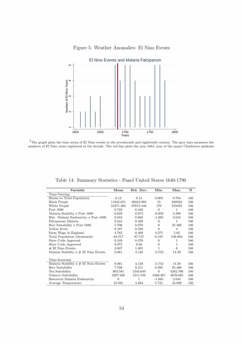
Figure 5: Weather Anomalies: El Nino Events

12

34

5N

umbe

r of

El N

ino

Yea

rs

1600 1650 1700 1750 1800Years

El Nino Events and Malaria Falciparum

†The graph plots the time series of El Nino events in the seventeenth and eighteenth century. The grey bars measures the

numbers of El Nino years registered in the decade. The red line plots the year 1684, year of the major Charleston epidemic.

Table 14: Summary Statistics - Panel United States 1640-1790

Variable Mean Std. Dev. Min. Max. NTime-VaryingBlacks to Total Population 0.12 0.15 0.003 0.704 166Black People 11845.651 30243.983 15 220582 166White People 52471.404 67674.448 170 319450 166Post 1690 0.723 0.449 0 1 166Malaria Stability x Post 1690 0.029 0.872 -0.959 2.398 166Hist. Malaria Endemicity x Post 1690 0.018 0.868 -1.065 2.044 166Falciparum Malaria 0.241 0.429 0 1 166Rice Suitability x Post 1690 5.706 8.076 0 25.466 166Yellow Fever 0.187 0.589 0 4 166Farm Wage in England 4.762 0.409 4.275 5.82 166Total Population (thousands) 64.317 87.747 0.185 538.004 166Slave Code Approval 0.349 0.478 0 1 166Slave Code Approved 0.072 0.26 0 1 166# El Nino Events 3.807 1.405 1 6 166Malaria Stability x # El Nino Events 0.061 4.128 -5.752 14.39 166

Time-InvariantMalaria Stability x # El Nino Events 0.061 4.128 -5.752 14.39 166Rice Suitability 7.708 8.311 0.295 25.466 166Tea Suitability 963.581 1344.649 0 4282.766 166Tobacco Suitability 3207.936 1211.556 1040.467 4670.695 166Historical Malaria Endemicity 0 1 -1.065 2.044 166Average Temperature 10.591 3.284 5.721 16.898 166

54

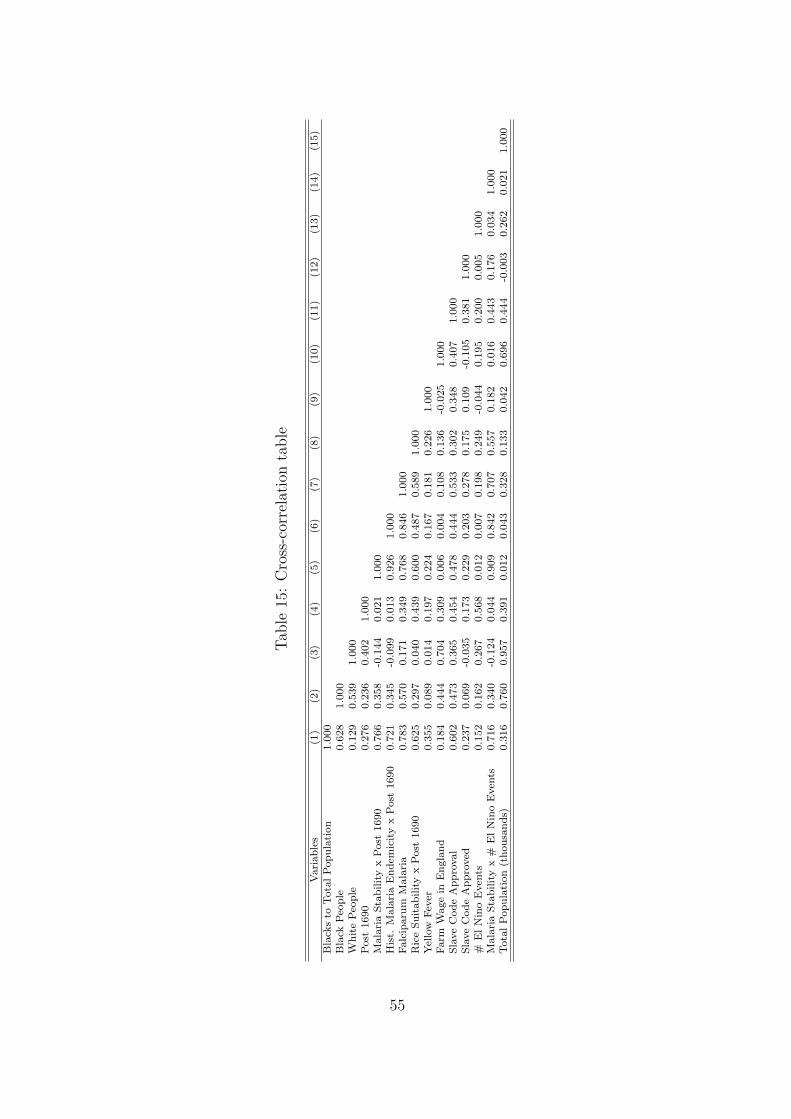
Tab

le15

:C

ross

-cor

rela

tion

table

Vari

ab

les

(1)

(2)

(3)

(4)

(5)

(6)

(7)

(8)

(9)

(10)

(11)

(12)

(13)

(14)

(15)

Bla

cks

toT

ota

lP

op

ula

tion

1.0

00

Bla

ckP

eop

le0.6

28

1.0

00

Wh

ite

Peo

ple

0.1

29

0.5

39

1.0

00

Post

1690

0.2

76

0.2

36

0.4

02

1.0

00

Mala

ria

Sta

bilit

yx

Post

1690

0.7

66

0.3

58

-0.1

44

0.0

21

1.0

00

His

t.M

ala

ria

En

dem

icit

yx

Post

1690

0.7

21

0.3

45

-0.0

99

0.0

13

0.9

26

1.0

00

Falc

iparu

mM

ala

ria

0.7

83

0.5

70

0.1

71

0.3

49

0.7

68

0.8

46

1.0

00

Ric

eS

uit

ab

ilit

yx

Post

1690

0.6

25

0.2

97

0.0

40

0.4

39

0.6

00

0.4

87

0.5

89

1.0

00

Yel

low

Fev

er0.3

55

0.0

89

0.0

14

0.1

97

0.2

24

0.1

67

0.1

81

0.2

26

1.0

00

Farm

Wage

inE

ngla

nd

0.1

84

0.4

44

0.7

04

0.3

09

0.0

06

0.0

04

0.1

08

0.1

36

-0.0

25

1.0

00

Sla

ve

Cod

eA

pp

roval

0.6

02

0.4

73

0.3

65

0.4

54

0.4

78

0.4

44

0.5

33

0.3

02

0.3

48

0.4

07

1.0

00

Sla

ve

Cod

eA

pp

roved

0.2

37

0.0

69

-0.0

35

0.1

73

0.2

29

0.2

03

0.2

78

0.1

75

0.1

09

-0.1

05

0.3

81

1.0

00

#E

lN

ino

Even

ts0.1

52

0.1

62

0.2

67

0.5

68

0.0

12

0.0

07

0.1

98

0.2

49

-0.0

44

0.1

95

0.2

00

0.0

05

1.0

00

Mala

ria

Sta

bilit

yx

#E

lN

ino

Even

ts0.7

16

0.3

40

-0.1

24

0.0

44

0.9

09

0.8

42

0.7

07

0.5

57

0.1

82

0.0

16

0.4

43

0.1

76

0.0

34

1.0

00

Tota

lP

op

ula

tion

(th

ou

san

ds)

0.3

16

0.7

60

0.9

57

0.3

91

0.0

12

0.0

43

0.3

28

0.1

33

0.0

42

0.6

96

0.4

44

-0.0

03

0.2

62

0.0

21

1.0

00

55

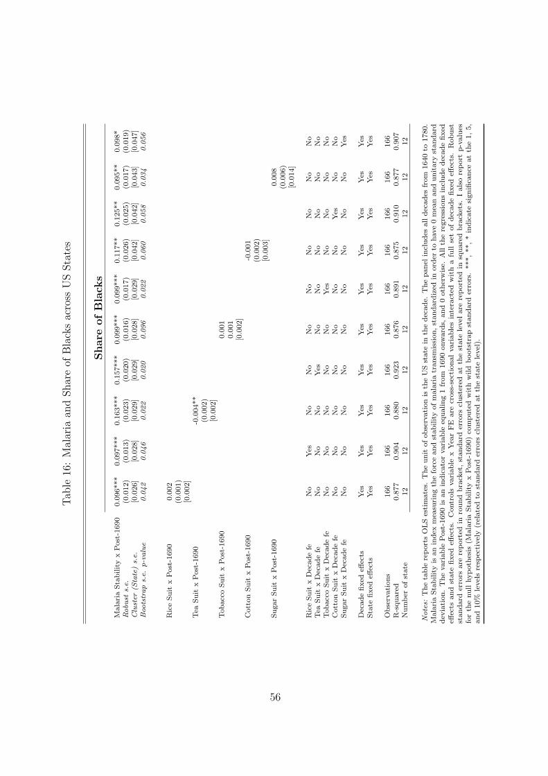
Tab

le16

:M

alar

iaan

dShar

eof

Bla

cks

acro

ssU

SSta

tes

Share

ofBlack

s

Mala

ria

Sta

bilit

yx

Post

-1690

0.0

96***

0.0

97***

0.1

63***

0.1

57***

0.0

99***

0.0

99***

0.1

17**

0.1

25**

0.0

95**

0.0

98*

Robu

sts.e.

(0.0

12)

(0.0

13)

(0.0

23)

(0.0

20)

(0.0

16)

(0.0

17)

(0.0

26)

(0.0

25)

(0.0

17)

(0.0

19)

Cluster

(State)s.e.

[0.0

26]

[0.0

28]

[0.0

29]

[0.0

29]

[0.0

28]

[0.0

29]

[0.0

42]

[0.0

42]

[0.0

43]

[0.0

47]

Boo

tstraps.e.

p-value

0.042

0.046

0.022

0.020

0.096

0.022

0.060

0.058

0.034

0.056

Ric

eS

uit

xP

ost

-1690

0.0

02

(0.0

01)

[0.0

02]

Tea

Su

itx

Post

-1690

-0.0

04**

(0.0

02)

[0.0

02]

Tob

acc

oS

uit

xP

ost

-1690

0.0

01

0.0

01

[0.0

02]

Cott

on

Su

itx

Post

-1690

-0.0

01

(0.0

02)

[0.0

03]

Su

gar

Su

itx

Post

-1690

0.0

08

(0.0

06)

[0.0

14]

Ric

eS

uit

xD

ecad

efe

No

Yes

No

No

No

No

No

No

No

No

Tea

Su

itx

Dec

ad

efe

No

No

No

Yes

No

No

No

No

No

No

Tob

acc

oS

uit

xD

ecad

efe

No

No

No

No

No

Yes

No

No

No

No

Cott

on

Su

itx

Dec

ad

efe

No

No

No

No

No

No

No

Yes

No

No

Su

gar

Su

itx

Dec

ad

efe

No

No

No

No

No

No

No

No

No

Yes

Dec

ad

efi

xed

effec

tsY

esY

esY

esY

esY

esY

esY

esY

esY

esY

esS

tate

fixed

effec

tsY

esY

esY

esY

esY

esY

esY

esY

esY

esY

es

Ob

serv

ati

on

s166

166

166

166

166

166

166

166

166

166

R-s

qu

are

d0.8

77

0.9

04

0.8

80

0.9

23

0.8

76

0.8

91

0.8

75

0.9

10

0.8

77

0.9

07

Nu

mb

erof

state

12

12

12

12

12

12

12

12

12

12

Notes:

Th

eta

ble

rep

ort

sO

LS

esti

mate

s.T

he

un

itof

ob

serv

ati

on

isth

eU

Sst

ate

inth

ed

ecad

e.T

he

pan

elin

clud

esall

dec

ad

esfr

om

1640

to1780.

Mala

ria

Sta

bilit

yis

an

ind

exm

easu

rin

gth

efo

rce

an

dst

ab

ilit

yof

mala

ria

tran

smis

sion

,st

an

dard

ized

inord

erto

have

0m

ean

an

du

nit

ary

stan

dard

dev

iati

on

.T

he

vari

ab

leP

ost

-1690

isan

ind

icato

rvari

ab

leeq

ualin

g1

from

1690

onw

ard

s,an

d0

oth

erw

ise.

All

the

regre

ssio

ns

incl

ud

ed

ecad

efi

xed

effec

tsan

dst

ate

fixed

effec

ts.

Contr

ols

vari

ab

lex

Yea

rF

Eare

cross

-sec

tion

al

vari

ab

les

inte

ract

edw

ith

afu

llse

tof

dec

ad

efi

xed

effec

ts.

Rob

ust

stan

dard

erro

rsare

rep

ort

edin

rou

nd

bra

cket

,st

an

dard

erro

rscl

ust

ered

at

the

state

level

are

rep

ort

edin

squ

are

db

rack

ets.

Ials

ore

port

p-v

alu

esfo

rth

enu

llhyp

oth

esis

(Mala

ria

Sta

bilit

yx

Post

-1690)

com

pu

ted

wit

hw

ild

boots

trap

stan

dard

erro

rs.

***,

**,

*in

dic

ate

sign

ifica

nce

at

the

1,

5,

an

d10%

level

sre

spec

tivel

y(r

elate

dto

stan

dard

erro

rscl

ust

ered

at

the

state

level

).

56

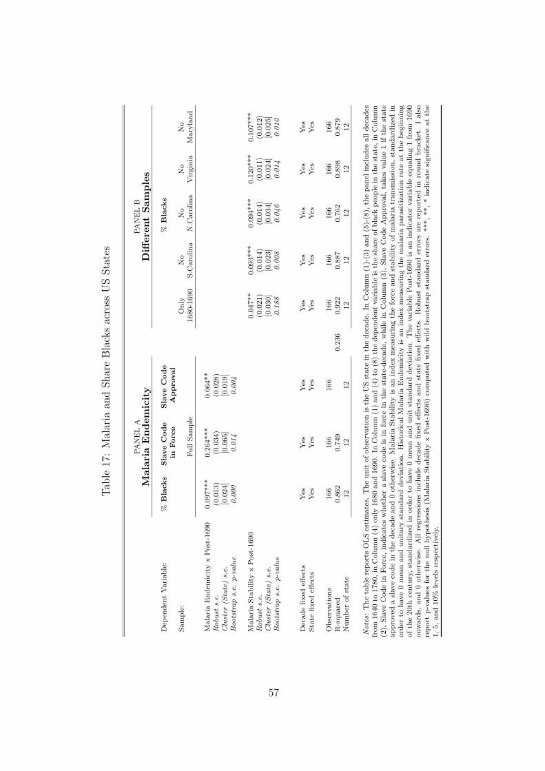
Tab

le17

:M

alar

iaan

dShar

eB

lack

sac

ross

US

Sta

tes

PA

NE

LA

PA

NE

LB

Mala

ria

En

dem

icit

yD

iffere

nt

Sam

ple

s

Dep

end

ent

Vari

ab

le:

%B

lacks

Sla

ve

Cod

eS

lave

Cod

e%

Bla

cks

inForce

App

roval

Sam

ple

:O

nly

No

No

No

No

Fu

llS

am

ple

1680-1

690

S.C

aro

lin

aN

.Caro

lin

aV

irgin

iaM

ary

lan

d

Mala

ria

En

dem

icit

yx

Post

-1690

0.0

97***

0.2

64***

0.0

64**

Robu

sts.e.

(0.0

13)

(0.0

34)

(0.0

28)

Cluster

(State)s.e.

[0.0

24]

[0.0

65]

[0.0

19]

Boo

tstraps.e.

p-value

0.000

0.014

0.004

Mala

ria

Sta

bilit

yx

Post

-1690

0.0

47**

0.0

93***

0.0

94***

0.1

20***

0.1

07***

Robu

sts.e.

(0.0

21)

(0.0

14)

(0.0

14)

(0.0

11)

(0.0

12)

Cluster

(State)s.e.

[0.0

30]

[0.0

23]

[0.0

34]

[0.0

24]

[0.0

25]

Boo

tstraps.e.

p-value

0.188

0.008

0.046

0.014

0.010

Dec

ad

efi

xed

effec

tsY

esY

esY

esY

esY

esY

esY

esY

esS

tate

fixed

effec

tsY

esY

esY

esY

esY

esY

esY

esY

es

Ob

serv

ati

on

s166

166

166

166

166

166

166

166

R-s

qu

are

d0.8

62

0.7

49

0.2

36

0.9

22

0.8

87

0.7

62

0.8

98

0.8

79

Nu

mb

erof

state

12

12

12

12

12

12

12

12

Notes:

Th

eta

ble

rep

ort

sO

LS

esti

mate

s.T

he

un

itof

ob

serv

ati

on

isth

eU

Sst

ate

inth

ed

ecad

e.In

Colu

mn

(1)-

(3)

an

d(5

)-(8

),th

ep

an

elin

clu

des

all

dec

ad

esfr

om

1640

to1780,

inC

olu

mn

(4)

on

ly1680

an

d1690.

InC

olu

mn

(1)

an

d(4

)to

(8)

the

dep

end

ent

vari

ab

leis

the

share

of

bla

ckp

eop

lein

the

state

,in

Colu

mn

(2),

Sla

ve

Cod

ein

Forc

e,in

dic

ate

sw

het

her

asl

ave

cod

eis

info

rce

inth

est

ate

-dec

ad

e,w

hile

inC

olu

mn

(3),

Sla

ve

Cod

eA

pp

roval,

takes

valu

e1

ifth

est

ate

ap

pro

ved

asl

ave

cod

ein

the

dec

ad

ean

d0

oth

erw

ise.

Mala

ria

Sta

bilit

yis

an

ind

exm

easu

rin

gth

efo

rce

an

dst

ab

ilit

yof

mala

ria

tran

smis

sion

,st

an

dard

ized

inord

erto

have

0m

ean

an

du

nit

ary

stan

dard

dev

iati

on

.H

isto

rica

lM

ala

ria

En

dem

icit

yis

an

ind

exm

easu

ring

the

mala

ria

para

siti

zati

on

rate

at

the

beg

inn

ing

of

the

20th

centu

ry,

stan

dard

ized

inord

erto

have

0m

ean

an

du

nit

stan

dard

dev

iati

on

.T

he

vari

ab

leP

ost

-1690

isan

ind

icato

rvari

ab

leeq

ualin

g1

from

1690

onw

ard

s,an

d0

oth

erw

ise.

All

regre

ssio

ns

incl

ud

ed

ecad

efi

xed

effec

tsan

dst

ate

fixed

effec

ts.

Rob

ust

stan

dard

erro

rsare

rep

ort

edin

rou

nd

bra

cket

.I

als

ore

port

p-v

alu

esfo

rth

enu

llhyp

oth

esis

(Mala

ria

Sta

bilit

yx

Post

-1690)

com

pu

ted

wit

hw

ild

boots

trap

stan

dard

erro

rs.

***,

**,

*in

dic

ate

sign

ifica

nce

at

the

1,

5,

an

d10%

level

sre

spec

tivel

y.

57

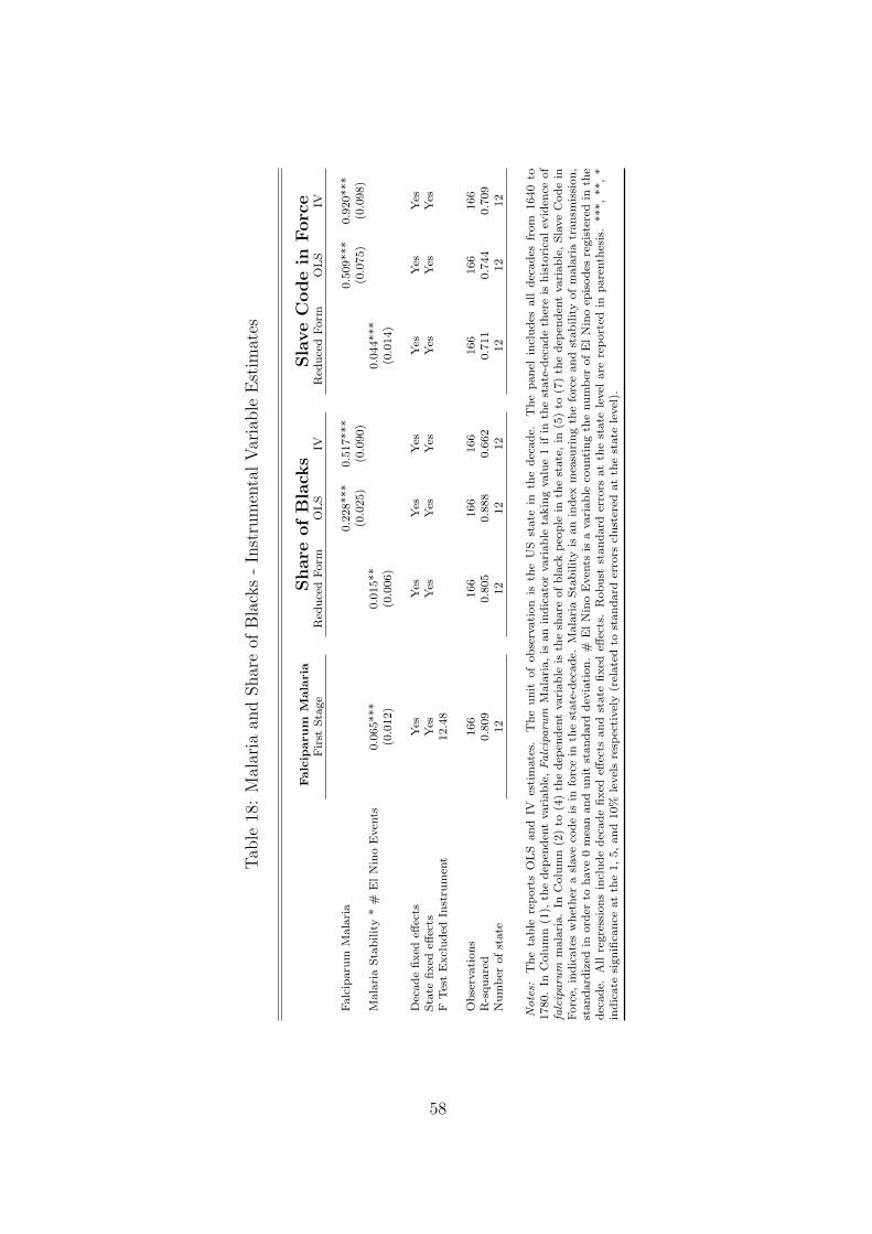
Tab

le18

:M

alar

iaan

dShar

eof

Bla

cks

-In

stru

men

tal

Var

iable

Est

imat

es

Falc

iparu

mM

ala

ria

Share

ofBlack

sSlaveCodein

Force

Fir

stS

tage

Red

uce

dF

orm

OL

SIV

Red

uce

dF

orm

OL

SIV

Falc

iparu

mM

ala

ria

0.2

28***

0.5

17***

0.5

09***

0.9

20***

(0.0

25)

(0.0

90)

(0.0

75)

(0.0

98)

Mala

ria

Sta

bilit

y*

#E

lN

ino

Even

ts0.0

65***

0.0

15**

0.0

44***

(0.0

12)

(0.0

06)

(0.0

14)

Dec

ad

efi

xed

effec

tsY

esY

esY

esY

esY

esY

esY

esS

tate

fixed

effec

tsY

esY

esY

esY

esY

esY

esY

esF

Tes

tE

xcl

ud

edIn

stru

men

t12.4

8

Ob

serv

ati

on

s166

166

166

166

166

166

166

R-s

qu

are

d0.8

09

0.8

05

0.8

88

0.6

62

0.7

11

0.7

44

0.7

09

Nu

mb

erof

state

12

12

12

12

12

12

12

Notes:

Th

eta

ble

rep

ort

sO

LS

an

dIV

esti

mate

s.T

he

un

itof

ob

serv

ati

on

isth

eU

Sst

ate

inth

ed

ecad

e.T

he

pan

elin

clu

des

all

dec

ad

esfr

om

1640

to1780.

InC

olu

mn

(1),

the

dep

end

ent

vari

ab

le,Falciparu

mM

ala

ria,

isan

ind

icato

rvari

ab

leta

kin

gvalu

e1

ifin

the

state

-dec

ad

eth

ere

ish

isto

rica

lev

iden

ceof

falciparu

mm

ala

ria.

InC

olu

mn

(2)

to(4

)th

ed

epen

den

tvari

ab

leis

the

share

of

bla

ckp

eop

lein

the

state

,in

(5)

to(7

)th

ed

epen

den

tvari

ab

le,

Sla

ve

Cod

ein

Forc

e,in

dic

ate

sw

het

her

asl

ave

cod

eis

info

rce

inth

est

ate

-dec

ad

e.M

ala

ria

Sta

bilit

yis

an

ind

exm

easu

rin

gth

efo

rce

an

dst

ab

ilit

yof

mala

ria

tran

smis

sion

,st

an

dard

ized

inord

erto

have

0m

ean

an

du

nit

stan

dard

dev

iati

on

.#

El

Nin

oE

ven

tsis

avari

ab

leco

unti

ng

the

nu

mb

erof

El

Nin

oep

isod

esre

gis

tere

din

the

dec

ad

e.A

llre

gre

ssio

ns

incl

ud

ed

ecad

efi

xed

effec

tsan

dst

ate

fixed

effec

ts.

Rob

ust

stan

dard

erro

rsat

the

state

level

are

rep

ort

edin

pare

nth

esis

.***,

**,

*in

dic

ate

sign

ifica

nce

at

the

1,

5,

an

d10%

level

sre

spec

tivel

y(r

elate

dto

stan

dard

erro

rscl

ust

ered

at

the

state

level

).

58

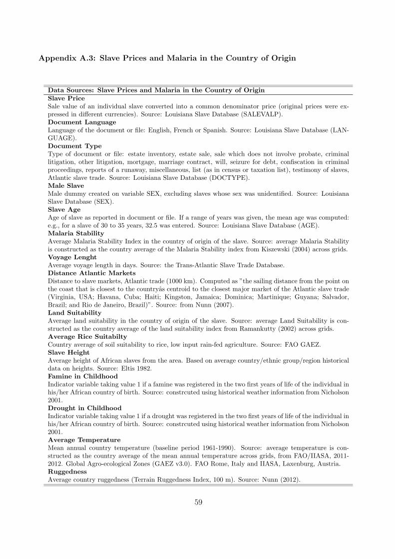
Appendix A.3: Slave Prices and Malaria in the Country of Origin

Data Sources: Slave Prices and Malaria in the Country of OriginSlave PriceSale value of an individual slave converted into a common denominator price (original prices were ex-pressed in different currencies). Source: Louisiana Slave Database (SALEVALP).Document LanguageLanguage of the document or file: English, French or Spanish. Source: Louisiana Slave Database (LAN-GUAGE).Document TypeType of document or file: estate inventory, estate sale, sale which does not involve probate, criminallitigation, other litigation, mortgage, marriage contract, will, seizure for debt, confiscation in criminalproceedings, reports of a runaway, miscellaneous, list (as in census or taxation list), testimony of slaves,Atlantic slave trade. Source: Louisiana Slave Database (DOCTYPE).Male SlaveMale dummy created on variable SEX, excluding slaves whose sex was unidentified. Source: LouisianaSlave Database (SEX).Slave AgeAge of slave as reported in document or file. If a range of years was given, the mean age was computed:e.g., for a slave of 30 to 35 years, 32.5 was entered. Source: Louisiana Slave Database (AGE).Malaria StabilityAverage Malaria Stability Index in the country of origin of the slave. Source: average Malaria Stabilityis constructed as the country average of the Malaria Stability index from Kiszewski (2004) across grids.Voyage LenghtAverage voyage length in days. Source: the Trans-Atlantic Slave Trade Database.Distance Atlantic MarketsDistance to slave markets, Atlantic trade (1000 km). Computed as ”the sailing distance from the point onthe coast that is closest to the countryas centroid to the closest major market of the Atlantic slave trade(Virginia, USA; Havana, Cuba; Haiti; Kingston, Jamaica; Dominica; Martinique; Guyana; Salvador,Brazil; and Rio de Janeiro, Brazil)”. Source: from Nunn (2007).Land SuitabilityAverage land suitability in the country of origin of the slave. Source: average Land Suitability is con-structed as the country average of the land suitability index from Ramankutty (2002) across grids.Average Rice SuitabiltyCountry average of soil suitability to rice, low input rain-fed agriculture. Source: FAO GAEZ.Slave HeightAverage height of African slaves from the area. Based on average country/ethnic group/region historicaldata on heights. Source: Eltis 1982.Famine in ChildhoodIndicator variable taking value 1 if a famine was registered in the two first years of life of the individual inhis/her African country of birth. Source: constrcuted using historical weather information from Nicholson2001.Drought in ChildhoodIndicator variable taking value 1 if a drought was registered in the two first years of life of the individual inhis/her African country of birth. Source: constrcuted using historical weather information from Nicholson2001.Average TemperatureMean annual country temperature (baseline period 1961-1990). Source: average temperature is con-structed as the country average of the mean annual temperature across grids, from FAO/IIASA, 2011-2012. Global Agro-ecological Zones (GAEZ v3.0). FAO Rome, Italy and IIASA, Laxenburg, Austria.RuggednessAverage country ruggedness (Terrain Ruggedness Index, 100 m). Source: Nunn (2012).

59

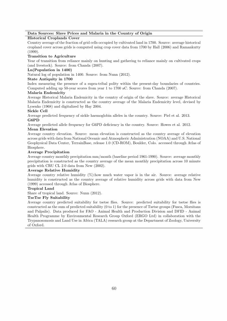
Data Sources: Slave Prices and Malaria in the Country of OriginHistorical Croplands CoverCountry average of the fraction of grid cells occupied by cultivated land in 1700. Source: average historicalcropland cover across grids is computed using crop cover data from 1700 by Hall (2006) and Ramankutty(1999).Transition to AgricultureYear of transition from reliance mainly on hunting and gathering to reliance mainly on cultivated crops(and livestock). Source: from Chanda (2007).Ln(Population in 1400)Natural log of population in 1400. Source: from Nunn (2012).State Antiquity in 1700Index measuring the presence of a supra-tribal polity within the present-day boundaries of countries.Computed adding up 50-year scores from year 1 to 1700 aC. Source: from Chanda (2007).Malaria EndemicityAverage Historical Malaria Endemicity in the country of origin of the slave. Source: average HistoricalMalaria Endemicity is constructed as the country average of the Malaria Endemicity level, devised byLysenko (1968) and digitalized by Hay 2004.Sickle CellAverage predicted frequency of sickle haemoglobin alleles in the country. Source: Piel et al. 2013.G6PDAverage predicted allele frequency for G6PD deficiency in the country. Source: Howes et al. 2012.Mean ElevationAverage country elevation. Source: mean elevation is constructed as the country average of elevationacross grids with data from National Oceanic and Atmospheric Administration (NOAA) and U.S. NationalGeophysical Data Center, TerrainBase, release 1.0 (CD-ROM), Boulder, Colo. accessed through Atlas ofBiosphere.Average PrecipitationAverage country monthly precipitation mm/month (baseline period 1961-1990). Source: average monthlyprecipitation is constructed as the country average of the mean monthly precipitation across 10 minutegrids with CRU CL 2.0 data from New (2002).Average Relative HumidityAverage country relative humidity (%):how much water vapor is in the air. Source: average relativehumidity is constructed as the country average of relative humidity across grids with data from New(1999) accessed through Atlas of Biosphere.Tropical LandShare of tropical land. Source: Nunn (2012).TseTse Fly SuitabilityAverage country predicted suitability for tsetse flies. Source: predicted suitability for tsetse flies isconstructed as the sum of predicted suitability (0 to 1) for the presence of Tsetse groups (Fusca, Morsitansand Palpalis). Data produced for FAO - Animal Health and Production Division and DFID - AnimalHealth Programme by Environmental Research Group Oxford (ERGO Ltd) in collaboration with theTrypanosomosis and Land Use in Africa (TALA) research group at the Department of Zoology, Universityof Oxford.

60

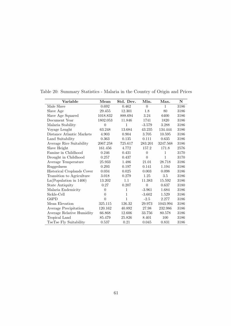
Table 20: Summary Statistics - Malaria in the Country of Origin and Prices

Variable Mean Std. Dev. Min. Max. NMale Slave 0.692 0.462 0 1 3186Slave Age 29.455 12.301 1.8 80 3186Slave Age Squared 1018.832 888.694 3.24 6400 3186Document Year 1802.053 11.846 1741 1820 3186Malaria Stability 0 1 -3.579 3.288 3186Voyage Lenght 63.248 13.684 43.235 134.444 3186Distance Atlantic Markets 4.903 0.904 3.705 10.595 3186Land Suitability 0.363 0.135 0.111 0.635 3186Average Rice Suitability 2067.258 725.617 283.201 3247.568 3186Slave Height 161.456 4.772 157.2 171.8 2576Famine in Childhood 0.246 0.431 0 1 3170Drought in Childhood 0.257 0.437 0 1 3170Average Temperature 25.933 1.486 21.01 28.718 3186Ruggedness 0.293 0.197 0.141 1.194 3186Historical Croplands Cover 0.034 0.025 0.003 0.098 3186Transition to Agriculture 3.018 0.279 1.25 3.5 3186Ln(Population in 1400) 13.202 1.1 11.383 15.592 3186State Antiquity 0.27 0.207 0 0.637 3180Malaria Endemicity 0 1 -3.961 1.684 3186Sickle-Cell 0 1 -3.602 1.529 3186G6PD 0 1 -2.5 2.277 3186Mean Elevation 325.115 126.32 29.973 1043.994 3186Average Precipitation 120.162 40.892 27.98 232.986 3186Average Relative Humidity 66.868 12.606 33.756 80.578 3186Tropical Land 85.479 25.826 8.401 100 3186TseTse Fly Suitability 0.537 0.21 0.045 0.831 3186

61

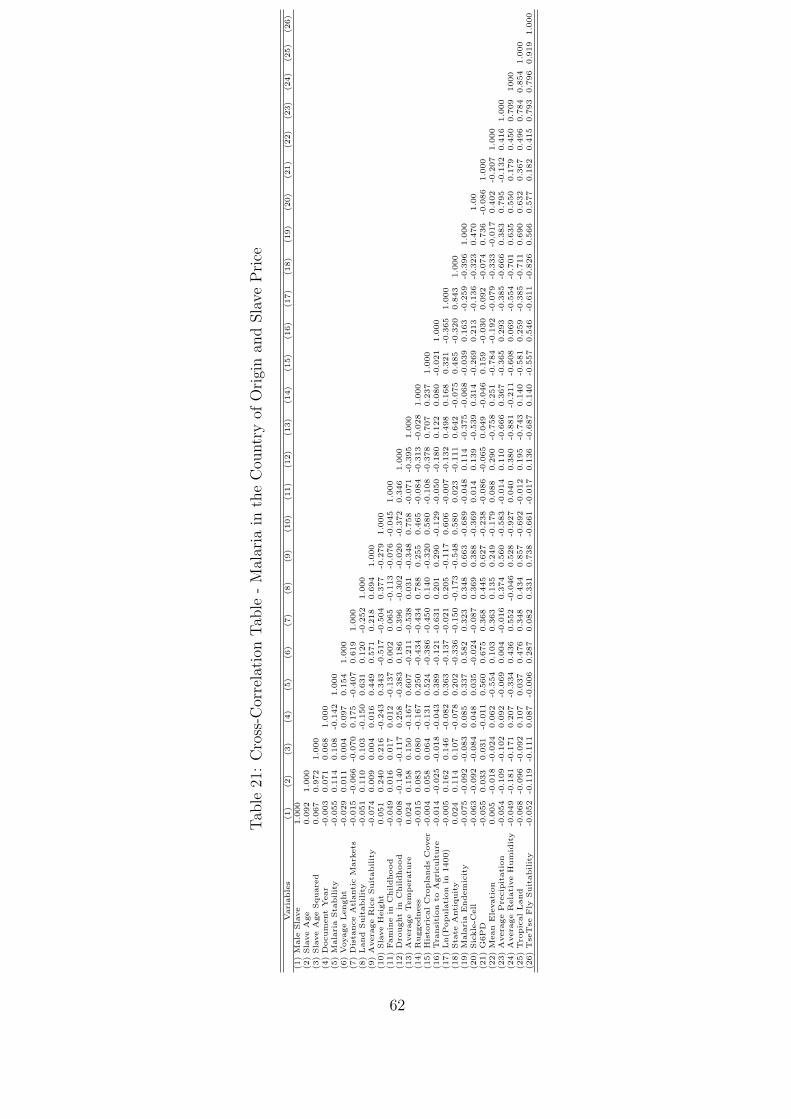
Tab

le21

:C

ross

-Cor

rela

tion

Tab

le-

Mal

aria

inth

eC

ountr

yof

Ori

gin

and

Sla

veP

rice

Variables

(1)

(2)

(3)

(4)

(5)

(6)

(7)

(8)

(9)

(10)

(11)

(12)

(13)

(14)

(15)

(16)

(17)

(18)

(19)

(20)

(21)

(22)

(23)

(24)

(25)

(26)

(1)M

ale

Slave

1.000

(2)SlaveAge

0.092

1.000

(3)SlaveAgeSquare

d0.067

0.972

1.000

(4)DocumentYear

-0.003

0.071

0.068

1.000

(5)M

alaria

Sta

bility

-0.055

0.114

0.108

-0.142

1.000

(6)VoyageLenght

-0.029

0.011

0.004

0.097

0.154

1.000

(7)Dista

nceAtlanticM

ark

ets

-0.015

-0.066

-0.070

0.175

-0.407

0.619

1.000

(8)Land

Suitability

-0.051

0.110

0.103

-0.150

0.631

0.120

-0.252

1.000

(9)Avera

geRiceSuitability

-0.074

0.009

0.004

0.016

0.449

0.571

0.218

0.694

1.000

(10)SlaveHeight

0.051

0.240

0.216

-0.243

0.343

-0.517

-0.504

0.377

-0.279

1.000

(11)Famin

ein

Childhood

-0.049

0.016

0.017

0.012

-0.137

0.002

0.065

-0.113

-0.076

-0.045

1.000

(12)Dro

ughtin

Childhood

-0.008

-0.140

-0.117

0.258

-0.383

0.186

0.396

-0.302

-0.020

-0.372

0.346

1.000

(13)Avera

geTempera

ture

0.024

0.158

0.150

-0.167

0.607

-0.211

-0.538

0.031

-0.348

0.758

-0.071

-0.395

1.000

(14)Ruggedness

-0.015

0.083

0.080

-0.167

0.250

-0.434

-0.434

0.788

0.255

0.465

-0.084

-0.313

-0.028

1.000

(15)Histo

ricalCro

plandsCover

-0.004

0.058

0.064

-0.131

0.524

-0.386

-0.450

0.140

-0.320

0.580

-0.108

-0.378

0.707

0.237

1.000

(16)Tra

nsition

toAgriculture

-0.014

-0.025

-0.018

-0.043

0.389

-0.121

-0.631

0.201

0.290

-0.129

-0.050

-0.180

0.122

0.080

-0.021

1.000

(17)Ln(P

opulation

in1400)

-0.005

0.162

0.146

-0.082

0.363

-0.137

-0.021

0.205

-0.117

0.606

-0.007

-0.132

0.498

0.168

0.321

-0.365

1.000

(18)Sta

teAntiquity

0.024

0.114

0.107

-0.078

0.202

-0.336

-0.150

-0.173

-0.548

0.580

0.023

-0.111

0.642

-0.075

0.485

-0.320

0.843

1.000

(19)M

alaria

Endemicity

-0.075

-0.092

-0.083

0.085

0.337

0.582

0.323

0.348

0.663

-0.689

-0.048

0.114

-0.375

-0.068

-0.039

0.163

-0.259

-0.396

1.000

(20)Sickle-C

ell

-0.063

-0.092

-0.084

0.048

0.035

-0.024

-0.087

0.369

0.388

-0.369

0.014

0.139

-0.539

0.314

-0.269

0.213

-0.136

-0.323

0.470

1.00

(21)G6PD

-0.055

0.033

0.031

-0.011

0.560

0.675

0.368

0.445

0.627

-0.238

-0.086

-0.065

0.049

-0.046

0.159

-0.030

0.092

-0.074

0.736

-0.086

1.000

(22)M

ean

Elevation

0.005

-0.018

-0.024

0.062

-0.554

0.103

0.363

0.135

0.249

-0.179

0.088

0.290

-0.758

0.251

-0.784

-0.192

-0.079

-0.333

-0.017

0.402

-0.207

1.000

(23)Avera

gePre

cip

itation

-0.054

-0.109

-0.102

0.092

-0.069

0.004

-0.016

0.374

0.560

-0.583

-0.014

0.110

-0.666

0.367

-0.365

0.293

-0.385

-0.666

0.383

0.795

-0.132

0.416

1.000

(24)Avera

geRelativeHumid

ity

-0.049

-0.181

-0.171

0.207

-0.334

0.436

0.552

-0.046

0.528

-0.927

0.040

0.380

-0.881

-0.211

-0.608

0.069

-0.554

-0.701

0.635

0.550

0.179

0.450

0.709

1000

(25)Tro

picalLand

-0.068

-0.096

-0.092

0.107

0.037

0.476

0.348

0.434

0.857

-0.692

-0.012

0.195

-0.743

0.140

-0.581

0.259

-0.385

-0.711

0.690

0.632

0.367

0.496

0.784

0.854

1.000

(26)Tse

Tse

Fly

Suitability

-0.052

-0.119

-0.111

0.087

-0.006

0.287

0.082

0.331

0.738

-0.661

-0.017

0.136

-0.687

0.140

-0.557

0.546

-0.611

-0.826

0.566

0.577

0.182

0.415

0.793

0.796

0.919

1.000

62

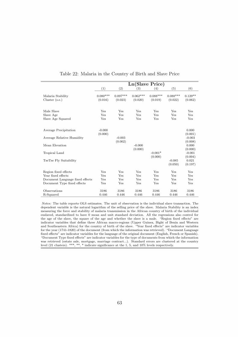
Table 22: Malaria in the Country of Birth and Slave Price

Ln(Slave Price)(1) (2) (3) (4) (5) (6)

Malaria Stability 0.080*** 0.097*** 0.062*** 0.088*** 0.088*** 0.129**Cluster (s.e.) (0.016) (0.023) (0.020) (0.019) (0.022) (0.062)

Male Slave Yes Yes Yes Yes Yes YesSlave Age Yes Yes Yes Yes Yes YesSlave Age Squared Yes Yes Yes Yes Yes Yes

Average Precipitation -0.000 0.000(0.000) (0.001)

Average Relative Humidity -0.003 -0.003(0.002) (0.008)

Mean Elevation -0.000 0.000(0.000) (0.000)

Tropical Land -0.001* -0.001(0.000) (0.004)

TseTse Fly Suitability -0.085 0.021(0.050) (0.197)

Region fixed effects Yes Yes Yes Yes Yes YesYear fixed effects Yes Yes Yes Yes Yes YesDocument Language fixed effects Yes Yes Yes Yes Yes YesDocument Type fixed effects Yes Yes Yes Yes Yes Yes

Observations 3186 3186 3186 3186 3186 3186R-Squared 0.446 0.446 0.446 0.446 0.446 0.446

Notes: The table reports OLS estimates. The unit of observation is the individual slave transaction. Thedependent variable is the natural logarithm of the selling price of the slave. Malaria Stability is an indexmeasuring the force and stability of malaria transmission in the African country of birth of the individualenslaved, standardized to have 0 mean and unit standard deviation. All the regressions also control forthe age of the slave, the square of the age and whether the slave is a male. “Region fixed effects” areindicator variables that define three African macro-regions (Upper Guinea, Bight of Benin and Westernand Southeastern Africa) for the country of birth of the slave. “Year fixed effects” are indicator variablesfor the year (1741-1820) of the document (from which the information was retrieved). “Document Languagefixed effects” are indicator variables for the language of the original document (English, French or Spanish).“Document Type fixed effects” are indicator variables for the type of documents from which the informationwas retrieved (estate sale, mortgage, marriage contract...). Standard errors are clustered at the countrylevel (21 clusters). ***, **, * indicate significance at the 1, 5, and 10% levels respectively.

63

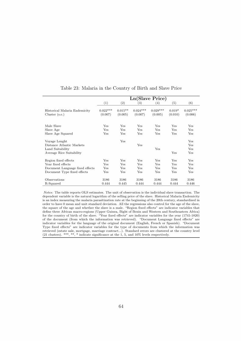
Table 23: Malaria in the Country of Birth and Slave Price

Ln(Slave Price)(1) (2) (3) (4) (5) (6)

Historical Malaria Endemicity 0.022*** 0.015** 0.024*** 0.029*** 0.019* 0.025***Cluster (s.e.) (0.007) (0.005) (0.007) (0.005) (0.010) (0.006)

Male Slave Yes Yes Yes Yes Yes YesSlave Age Yes Yes Yes Yes Yes YesSlave Age Squared Yes Yes Yes Yes Yes Yes

Voyage Lenght Yes YesDistance Atlantic Markets Yes YesLand Suitability Yes YesAverage Rice Suitability Yes Yes

Region fixed effects Yes Yes Yes Yes Yes YesYear fixed effects Yes Yes Yes Yes Yes YesDocument Language fixed effects Yes Yes Yes Yes Yes YesDocument Type fixed effects Yes Yes Yes Yes Yes Yes

Observations 3186 3186 3186 3186 3186 3186R-Squared 0.444 0.445 0.444 0.444 0.444 0.446

Notes: The table reports OLS estimates. The unit of observation is the individual slave transaction. Thedependent variable is the natural logarithm of the selling price of the slave. Historical Malaria Endemicityis an index measuring the malaria parasitization rate at the beginning of the 20th century, standardized inorder to have 0 mean and unit standard deviation. All the regressions also control for the age of the slave,the square of the age and whether the slave is a male. “Region fixed effects” are indicator variables thatdefine three African macro-regions (Upper Guinea, Bight of Benin and Western and Southeastern Africa)for the country of birth of the slave. “Year fixed effects” are indicator variables for the year (1741-1820)of the document (from which the information was retrieved). “Document Language fixed effects” areindicator variables for the language of the original document (English, French or Spanish). “DocumentType fixed effects” are indicator variables for the type of documents from which the information wasretrieved (estate sale, mortgage, marriage contract...). Standard errors are clustered at the country level(21 clusters). ***, **, * indicate significance at the 1, 5, and 10% levels respectively.

64

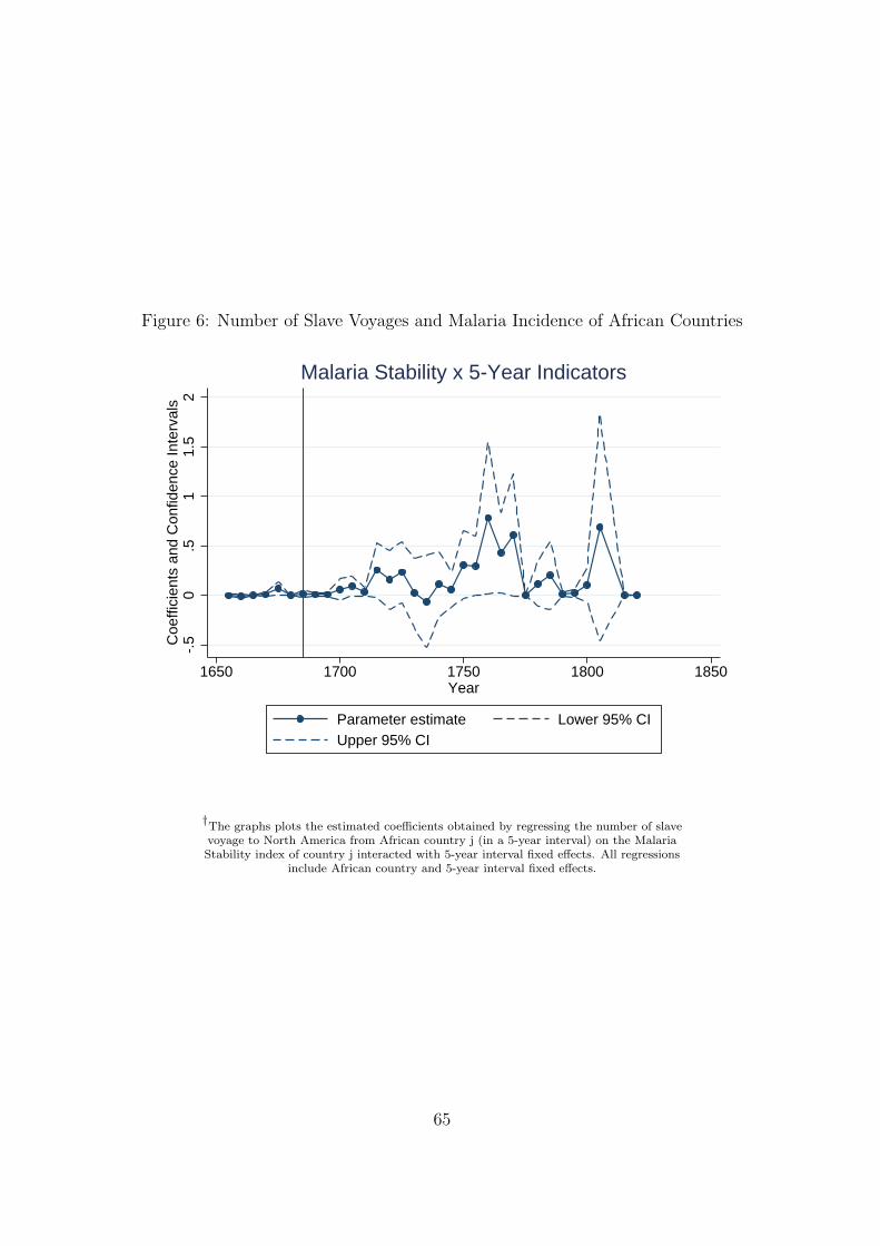
Figure 6: Number of Slave Voyages and Malaria Incidence of African Countries

-.5

0.5

11.

52

Coe

ffici

ents

and

Con

fiden

ce In

terv

als

1650 1700 1750 1800 1850Year

Parameter estimate Lower 95% CIUpper 95% CI

Malaria Stability x 5-Year Indicators

†The graphs plots the estimated coefficients obtained by regressing the number of slavevoyage to North America from African country j (in a 5-year interval) on the MalariaStability index of country j interacted with 5-year interval fixed effects. All regressions

include African country and 5-year interval fixed effects.

65

Tab

le24

:M

alar

iain

the

Cou

ntr

yof

Bir

than

dSla

veP

rice

Ln(S

lavePrice

)SlavePrice

No

Bord

er

Grou

ps

No

“C

on

go”

No

“G

uin

ea”

Fu

llS

am

ple

(1)

(2)

(3)

(4)

(5)

(6)

(7)

(8)

Mala

ria

Sta

bilit

y0.0

75***

0.0

74***

0.0

72***

0.0

82***

0.0

69***

0.0

82***

36.7

46***

40.7

32***

Clu

ster

s.e.

(0.0

18)

(0.0

19)

(0.0

21)

(0.0

21)

(0.0

15)

(0.0

23)

(8.8

40)

(6.7

77)

Male

Sla

ve

Yes

Yes

Yes

Yes

Yes

Yes

Yes

Yes

Sla

ve

Age

Yes

Yes

Yes

Yes

Yes

Yes

Yes

Yes

Sla

ve

Age

Squ

are

dY

esY

esY

esY

esY

esY

esY

esY

es

Reg

ion

fixed

effec

tsY

esY

esY

esY

esY

esY

esY

esY

esY

ear

fixed

effec

tsY

esY

esY

esY

esY

esY

esY

esY

esD

ocu

men

tL

an

gu

age

fixed

effec

tsY

esY

esY

esY

esY

esY

esY

esY

esD

ocu

men

tT

yp

efi

xed

effec

tsY

esY

esY

esY

esY

esY

esY

esY

es

Ob

serv

ati

on

s1616

1616

1988

1988

2832

2832

3186

3186

R-S

qu

are

d0.4

49

0.4

51

0.4

43

0.4

45

0.4

50

0.4

51

0.3

63

0.3

65

Notes:

Th

eta

ble

rep

ort

sO

LS

esti

mate

s.T

he

un

itof

ob

serv

ati

on

isth

ein

div

idu

al

slave

tran

sact

ion

.T

he

dep

end

ent

vari

ab

leis

the

natu

ral

logari

thm

of

the

sellin

gp

rice

of

the

slave

inC

olu

mn

(1)

to(6

),an

dth

eab

solu

tevalu

eof

the

sale

pri

cein

Colu

mn

(7)

to(8

).M

ala

ria

Sta

bilit

yis

an

ind

exm

easu

rin

gth

efo

rce

an

dst

ab

ilit

yof

mala

ria

tran

smis

sion

inth

eA

fric

an

cou

ntr

yof

bir

thof

the

ind

ivid

ual

ensl

aved

,st

an

dard

ized

toh

ave

0m

ean

an

du

nit

stan

dard

dev

iati

on

.A

llth

ere

gre

ssio

ns

als

oco

ntr

ol

for

the

age

of

the

slave,

the

squ

are

of

the

age

an

dw

het

her

the

slave

isa

male

.“R

egio

nfi

xed

effec

ts”

are

ind

icato

rvari

ab

les

that

defi

ne

thre

eA

fric

an

macr

o-r

egio

ns

(Up

per

Gu

inea

,B

ight

of

Ben

inan

dW

este

rnan

dS

ou

thea

ster

nA

fric

a)

for

the

cou

ntr

yof

bir

thof

the

slave.

“Y

ear

fixed

effec

ts”

are

ind

icato

rvari

ab

les

for

the

yea

r(1

741-1

820)

of

the

docu

men

t(f

rom

wh

ich

the

info

rmati

on

was

retr

ieved

).“D

ocu

men

tL

an

gu

age

fixed

effec

ts”

are

ind

icato

rvari

ab

les

for

the

lan

gu

age

of

the

ori

gin

al

docu

men

t(E

nglish

,F

ren

chor

Sp

anis

h).

“D

ocu

men

tT

yp

efi

xed

effec

ts”

are

ind

icato

rvari

ab

les

for

the

typ

eof

docu

men

tsfr

om

wh

ich

the

info

rmati

on

was

retr

ieved

(est

ate

sale

,m

ort

gage,

marr

iage

contr

act

...)

.S

tan

dard

erro

rsare

clu

ster

edat

the

cou

ntr

yle

vel

(21

clu

ster

s).

***,

**,

*in

dic

ate

sign

ifica

nce

at

the

1,

5,

an

d10%

level

sre

spec

tivel

y.

66

Table 25: Malaria and Slave Mortality

Share of Deaths during Middle Passage(1) (2) (3) (4) (5)

Malaria Stability -0.004*** -0.009*** -0.010*** -0.009*** -0.006***(0.001) (0.002) (0.003) (0.003) (0.002)

Bootstrap s.e. p-value 0.040 0.004 0.002 0.018 0.066

Voyage Lenght Yes Yes Yes Yes YesRuggedness No Yes Yes Yes YesTemperature No No Yes Yes YesSoil No No No Yes YesLatitude No No No No Yes

Region fixed effects Yes Yes Yes Yes YesYear fixed effects Yes Yes Yes Yes Yes

Observations 3,951 3,951 3,951 3,951 3,951R-squared 0.267 0.271 0.271 0.271 0.275

Notes: The table reports OLS estimates. The unit of observation is the single AfricanTrade ship voyage. The dependent variable is the share of enslaved individuals dyingduring the voyage. Malaria Stability is an index measuring the force and stability ofmalaria transmission in the African country of embarkation.“Region fixed effects” areindicator variables that define African macro-regions (Upper Guinea, Bight of Benin,Western Africa and Southeastern Africa) for the country of birth of the slave. “Yearfixed effects” are indicator variables for the year of the sea voyage. Standard errors areclustered at the country level. Given the small number of clusters (17), I report p-valuesfor the null hypothesis, i.e. Malaria Stability = 0, computed with wild bootstrap standarderrors. ***, **, * indicate significance at 1, 5, and 10% levels, respectively.

Table 26: Malaria and Slave Exports in Africa

Ln(Slaves Exported over Total Area)(1) (2) (3) (4) (5)

Malaria Stability 0.262*** 0.205*** 0.217*** 0.162** 0.136**(0.030) (0.049) (0.044) (0.064) (0.065)

Ruggedness No Yes No Yes YesTemperature No Yes No Yes YesHumidity No Yes No Yes YesNear Coast No No Yes Yes YesDistances Slave Markets No No Yes Yes YesLn Pop Density 1400 No No No No Yes

Observations 57 47 57 47 47R-squared 0.471 0.483 0.560 0.526 0.604

Notes: The table reports OLS estimates. The unit of observation is the AfricanCountry. The dependent variable is the natural logarithm of the total number ofslaves exported over the total land area. Malaria Stability is an index measuring theforce and stability of malaria transmission. Robust standard errors in parenthesis.***, **, * indicate significance at 1, 5, and 10% levels respectively.

67

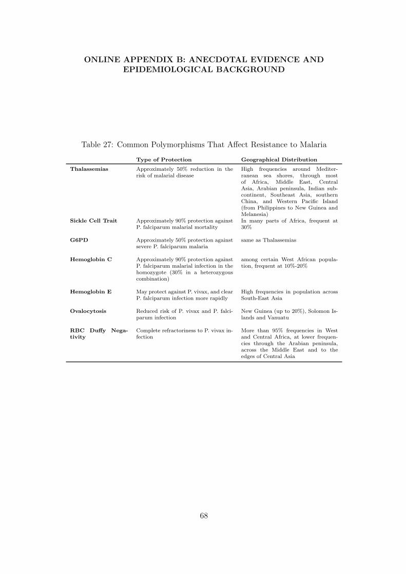
ONLINE APPENDIX B: ANECDOTAL EVIDENCE ANDEPIDEMIOLOGICAL BACKGROUND

Table 27: Common Polymorphisms That Affect Resistance to Malaria

Type of Protection Geographical Distribution

Thalassemias Approximately 50% reduction in therisk of malarial disease

High frequencies around Mediter-ranean sea shores, through mostof Africa, Middle East, CentralAsia, Arabian peninsula, Indian sub-continent, Southeast Asia, southernChina, and Western Pacific Island(from Philippines to New Guinea andMelanesia)

Sickle Cell Trait Approximately 90% protection againstP. falciparum malarial mortality

In many parts of Africa, frequent at30%

G6PD Approximately 50% protection againstsevere P. falciparum malaria

same as Thalassemias

Hemoglobin C Approximately 90% protection againstP. falciparum malarial infection in thehomozygote (30% in a heterozygouscombination)

among certain West African popula-tion, frequent at 10%-20%

Hemoglobin E May protect against P. vivax, and clearP. falciparum infection more rapidly

High frequencies in population acrossSouth-East Asia

Ovalocytosis Reduced risk of P. vivax and P. falci-parum infection

New Guinea (up to 20%), Solomon Is-lands and Vanuatu

RBC Duffy Nega-tivity

Complete refractoriness to P. vivax in-fection

More than 95% frequencies in Westand Central Africa, at lower frequen-cies through the Arabian peninsula,across the Middle East and to theedges of Central Asia

68

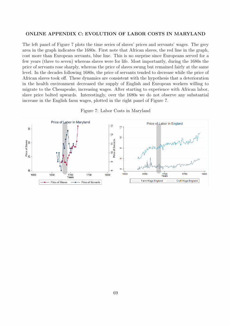
ONLINE APPENDIX C: EVOLUTION OF LABOR COSTS IN MARYLAND

The left panel of Figure 7 plots the time series of slaves’ prices and servants’ wages. The greyarea in the graph indicates the 1680s. First note that African slaves, the red line in the graph,cost more than European servants, blue line. This is no surprise since Europeans served for afew years (three to seven) whereas slaves were for life. Most importantly, during the 1680s theprice of servants rose sharply, whereas the price of slaves swung but remained fairly at the samelevel. In the decades following 1680s, the price of servants tended to decrease while the price ofAfrican slaves took off. These dynamics are consistent with the hypothesis that a deteriorationin the health environment decreased the supply of English and European workers willing tomigrate to the Chesapeake, increasing wages. After starting to experience with African labor,slave price bolted upwards. Interestingly, over the 1680s we do not observe any substantialincrease in the English farm wages, plotted in the right panel of Figure 7.

Figure 7: Labor Costs in Maryland

69

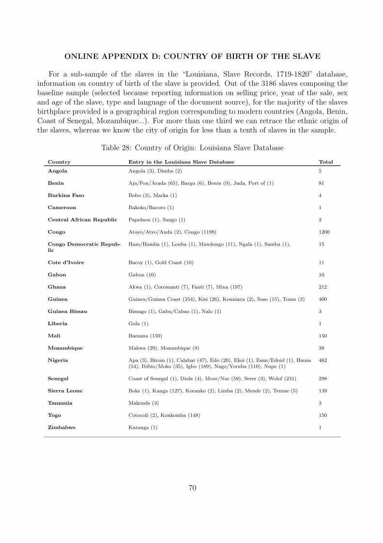
ONLINE APPENDIX D: COUNTRY OF BIRTH OF THE SLAVE

For a sub-sample of the slaves in the “Louisiana, Slave Records, 1719-1820” database,information on country of birth of the slave is provided. Out of the 3186 slaves composing thebaseline sample (selected because reporting information on selling price, year of the sale, sexand age of the slave, type and language of the document source), for the majority of the slavesbirthplace provided is a geographical region corresponding to modern countries (Angola, Benin,Coast of Senegal, Mozambique...). For more than one third we can retrace the ethnic origin ofthe slaves, whereas we know the city of origin for less than a tenth of slaves in the sample.

Table 28: Country of Origin: Louisiana Slave Database

Country Entry in the Louisiana Slave Database Total

Angola Angola (3), Dimba (2) 5

Benin Aja/Fon/Arada (65), Bargu (6), Benin (9), Juda, Port of (1) 81

Burkina Faso Bobo (3), Marka (1) 4

Cameroon Bakoko/Bacoro (1) 1

Central African Republic Papelaou (1), Sango (1) 2

Congo Atoyo/Atyo/Auda (2), Congo (1198) 1200

Congo Democratic Repub-lic

Ham/Hamba (1), Louba (1), Mandongo (11), Ngala (1), Samba (1), 15

Cote d’Ivoire Bacoy (1), Gold Coast (10) 11

Gabon Gabon (10) 10

Ghana Akwa (1), Coromanti (7), Fanti (7), Mina (197) 212

Guinea Guinea/Guinea Coast (354), Kisi (26), Kouniaca (2), Soso (15), Toma (3) 400

Guinea Bissau Bissago (1), Gabu/Cabao (1), Nalo (1) 3

Liberia Gola (1) 1

Mali Bamana (150) 150

Mozambique Makwa (29), Mozambique (9) 38

Nigeria Apa (3), Birom (1), Calabar (47), Edo (20), Ekoi (1), Esan/Edoid (1), Hausa(54), Ibibio/Moko (35), Igbo (189), Nago/Yoruba (110), Nupe (1)

462

Senegal Coast of Senegal (1), Diola (4), Moor/Nar (59), Serer (3), Wolof (231) 298

Sierra Leone Boke (1), Kanga (127), Koranko (2), Limba (2), Mende (2), Temne (5) 139

Tanzania Makonde (3) 3

Togo Cotocoli (2), Konkomba (148) 150

Zimbabwe Karanga (1) 1

70

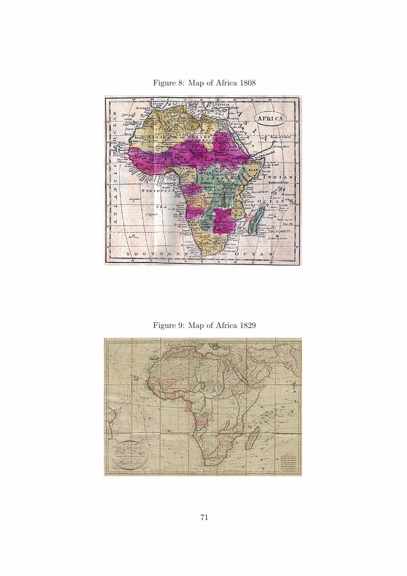
Figure 8: Map of Africa 1808

Figure 9: Map of Africa 1829

71

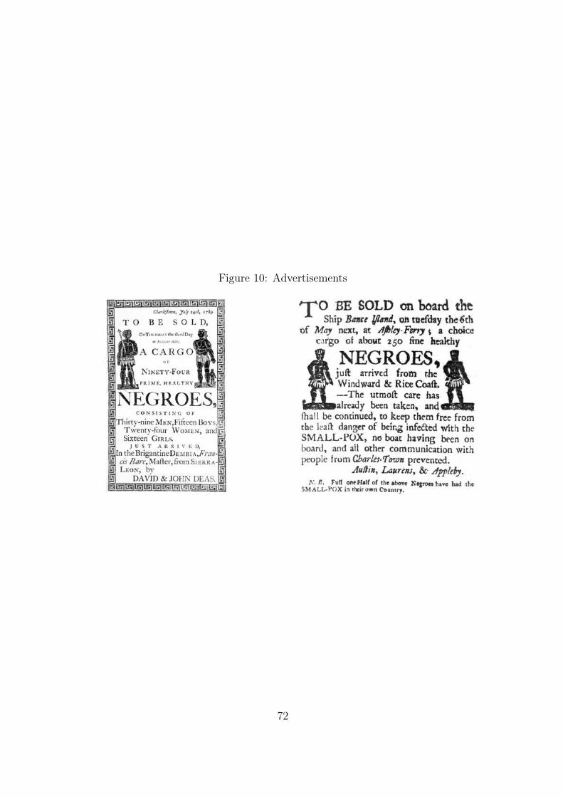
Figure 10: Advertisements

72