i

NUMERICAL APPROXIMATION IN CFD PROBLEMS

USING PHYSICS INFORMED MACHINE LEARNING

A Thesis

Submitted by

SIDDHARTH ROUT

for the award of the degree

of

BACHELOR OF TECHNOLOGY

&

MASTER OF TECHNOLOGY

DEPARTMENT OF MECHANICAL ENGINEERING

INDIAN INSTITUTE OF TECHNOLOGY MADRAS

CHENNAI-600036

MAY 2019

ii

iii

Jai Jagannath

iv

THESIS CERTIFICATE

This is to certify that the thesis entitled “Numerical Approximation in CFD Problems Using

Physics Informed Machine Learning” submitted by Siddharth Rout to the Indian Institute

of Technology, Madras for the award of B. Tech – M. Tech Dual Degree is a bona fide record

of research work carried out by him under my supervision. The contents of this thesis, in full

or in parts, have not been submitted to any other Institute or University for the award of any

degree or diploma.

Prof. Balaji Srinivasan

Associate Professor

Department of Mechanical Engineering

Indian Institute of Technology Madras

Chennai – 600 036.

Place: Chennai

Date: May 2019

i

ACKNOWLEDGEMENTS

My father often says, “Every one of us needs a good mentor and back support to achieve

something in life. A good mentor is a privilege and privileges should always be respected.” It

gives me a sense of satisfaction to express my sincere gratitude to my supervisor Dr. Balaji

Srinivasan for being a mentor and guide to me in true sense. He is the most sensible person I

have ever met. He has given a direction to my career. I would like to thank him for introducing

me to the exciting field of applied machine learning in fluid mechanics. I would like to thank

God for putting me at the right place. It is a privilege to be part of his research team.

I would like to thank my lab mate Vikas Dwivedi for being a constant support throughout the

last year. We have spent hours and days discussing various problems or test results which we

encountered during the course of the project. No matter if we got the right or wrong solution,

that helped us to stay motivated.

ii

ABSTRACT

Keywords: Numerical approximation; Advection-Diffusion Equation; Advection Dominant

Flows; Neural Networks; Physics Informed Learning; Extreme Learning Machine.

The thesis focuses on various techniques to find an alternate approximation method that could

be universally used for a wide range of CFD problems but with low computational cost and

low runtime. Various techniques have been explored within the field of machine learning to

gauge the utility in fulfilling the core ambition. Steady advection diffusion problem has been

used as the test case to understand the level of complexity up to which a method can provide

solution. Ultimately, the focus stays over physics informed machine learning techniques where

solving differential equations is possible without any training with computed data. The

prevalent methods by I.E. Lagaris et.al. and M. Raissi et.al are explored thoroughly.

The prevalent methods cannot solve advection dominant problems. A physics informed

method, called as Distributed Physics Informed Neural Network (DPINN), is proposed to solve

advection dominant problems. It increases the flexibility and capability of older methods by

splitting the domain and introducing other physics-based constraints as mean squared loss

terms. Various experiments are done to explore the end to end possibilities with the method.

Parametric study is also done to understand the behavior of the method to different tunable

parameters. The method is tested over steady advection-diffusion problems and unsteady

square pulse problems. Very accurate results are recorded.

Extreme learning machine (ELM) is a very fast neural network algorithm at the cost of tunable

parameters. The ELM based variant of the proposed model is tested over the advection-

diffusion problem. ELM makes the complex optimization simpler and since the method is non-

iterative, the solution is recorded in a single shot. The ELM based variant seems to work better

than the simple DPINN method. Simultaneously scope for various development in future are

hinted throughout the thesis.

iii

TABLE OF CONTENTS

ABSTRACT ii

TABLE OF CONTENTS iii

LIST OF FIGURES vii

LIST OF TABLES viiiiii

CHAPTER 1

INTRODUCTION

1.1. INTRODUCTION 9

1.2. OBJECTIVE OF THE WORK 10

1.3. ARTIFICIAL NEURAL NETWORKS 10

1.4. NEURAL NETWORKS AS FUNCTION APPROXIMATORS 12

1.5. THE PROBLEM WITH ADVECTION-DIFFUSION 13

CHAPTER 2

DATA DRIVEN METHODS

2.1.1. NON-LINEAR REGRESSION OF PHYSICAL SOLUTION FOR

ADVECTION-DIFFUSION EQUATION 14

2.1.2. OBSERVATIONS 15

2.2.1. ENHANCEMENT OF SOLUTION FROM CENTRAL DIFFERENCE SCHEME

17

2.2.2. OBSERVATIONS 19

2.3.1. PREDICTION OF ERROR IN CDS SOLUTION 19

2.3.2. OBSERVATIONS 19

2.4. FUNCTION APPROXIMATION OF EXACT PHYSICAL SOLUTION 19

2.5. CONCLUSION 19

CHAPTER 3

PHYSICS INFORMED LEARNING

3.1. PHYSICS INFORMED NEURAL NETWORK FOR SOLVING ODE AND PDE

20

3.2.1 LAGARIS’ ALGORITHM 20

3.2.2. LAGARIS’ IMPLEMENTATION OF ADVECTION-DIFFUSION 21

3.3.1. PHYSICS INFORMED DEEP LEARNING BY MAZIAR RAISSI ET. AL. 22

iv

3.3.2. PINN IMPLEMENTATION FOR ADVECTION-DIFFUSION 23

CHAPTER 4

DISTRIBUTED PHYSICS INFORMED NEURAL NETWORK (DPINN)

4.1. INTRODUCTION 24

4.2. DATA DRIVEN DISTRIBUTED NEURAL NETWORK 24

4.3. DISTRIBUTED PHYSICS INFORMED NEURAL NETWORK (DPINN) 25

4.4.1. INTERFACE CONDITIONS: VALUE MATCHING 26

4.4.2. INTERFACE CONDITIONS: SLOPE MATCHING 26

4.4.3. INTERFACE CONDITIONS: SECOND DERIVATIVE MATCHING 27

4.4.4. INTERFACE CONDITIONS: FLUX MATCHING 27

4.5. DPINN IMPLEMENTATION OF STEADY ADVECTION-DIFFUSION 28

4.6. SUMMARY OF DPINN 29

CHAPTER 5

EXPERIMENTS TO ENHANCE DPINN

5.1. INTRODUCTION 30

5.2. RANDOM COLLOCATION POINTS FOR FORCING THE EQUATION 30

5.3. EFFECTS OF ACTIVATION FUNCTIONS 30

5.4. REGULARIZATION 31

5.5.1. WEIGHED LOSS TERMS 32

5.5.2. TUNING WEIGHED LOSS TERMS BY TRIALS 33

5.5.3. LAGRANGIAN MULTIPLIERS FOR CONSTRAINED OPTIMIZATION 34

5.6. WEIGHT INITIALIZATION BY RECURRENT DOMAIN SPLIT 35

5.7. GUIDED CONVERGENCE BY UPDATING 𝜖 THROUGH ITERATION 36

5.8.1. MODIFIED TRIAL FUNCTIONS WITH EXTRA LINEAR COMPONENT 37

5.8.2. MODIFIED TRIAL FUNCTIONS FOR BOUNDARY FORCING 37

5.8.3. MODIFIED TRIAL FUNCTIONS FOR FORCING BOUNDARIES AND

INTERFACE MATCHING 38

5.9. EFFECT OF NEGATIVE ‘𝜖’ AND DOMAIN OF ‘X’ 39

5.10. USING THE FLUX TERM FOR FORCING AT COLLOCATION POINTS 40

5.11. LOSS TERM TREND WITH ITERATION 41

5.12. LOSS GRADIENT TREND WITH ITERATION 43

5.13. NORMALIZATION OF EACH SUB-DOMAIN IN DPINN 44

v

5.14. TESTS FOR FINDING ISSUES 46

5.14.1.PIECEWISE LINEAR APPROXIMATION 46

5.14.2.PIECEWISE QUADRATIC APPROXIMATION 48

5.14.3.CONCLUSION FROM EQUATION SOLVING 49

5.15. LEVENBERG-MARQUARDT ALGORITHM FOR WEIGHT UPDATE 50

CHAPTER 6

EXTREME LEARNING MACHINE BASED DPINN

6.1. EXTREME LEARNING MACHINE 52

6.2.1. ELM IN PINN FOR ADVECTION-DIFFUSION 53

6.2.2. OBSERVATIONS 54

6.3.1. ELM IN DISTRIBUTED PINN 56

6.3.2. OBSERVATIONS 57

6.4. NORMALIZATION OF ELM BASED DPINN 60

CHAPTER 7

PARAMETRIC STUDY: 1-D UNSTEADY ADVECTION USING DPINN

7.1. EFFECT OF NUMBER OF BLOCKS 62

7.2. EFFECT OF COLLOCATION POINTS PER BLOCK 63

7.3. EFFECT OF LEARNING RATE 64

7.4. EFFECT OF OPTIMIZER 66

7.5. EFFECT OF NON-LINEARITY 67

7.6. EFFECT OF NUMBER OF NEURONS IN EACH LAYER 68

7.7. EFFECT OF NUMBER OF LAYERS 69

CHAPTER 8

CONCLUSIONS 71

RECOMMENDATIONS FOR FUTURE WORK 71

REFERENCES 72

vi

LIST OF FIGURES

Figure 1.1: Analogy between biological and artificial neuron

Figure 1.2: Deep neural network architecture.

Figure 1.3: Advection-diffusion solutions

Figure 2.1: Architecture for solution enhancement

Figure 2.2: Comparisons of neural network enhanced predictions vs upwind solution for

two cases

Figure 2.3: Effect of number of training data enhancement.

Figure 2.4: Prediction of exact solution by adding artificial diffusion.

Figure 2.5: Regression plot for prediction with the architecture [3, 50, 30, 1].

Figure 3.1: Comparison of prediction using Lagaris’ concept for ϵ = 0.3 and 0.7.

Figure 3.2: Prediction using PINN for ϵ = 0.15

Figure 4.1: Prediction using distributed neural network for ϵ = 0.03

Figure 4.2: Split of domain into blocks for a two-variable system

Figure 4.3: Neural network architecture for each block in DPINN for a specific case.

Figure 5.1: Weight matrices for different cases.

Figure 5.2: Predictions using DPINN for ϵ = 0.1 and ϵ = 0.075

Figure 5.3: Predictions using DPINN for different weights assigned to loss terms for ϵ =

0.05 and lr = 0.01

Figure 5.4: Predictions using DPINN for weights decided by trials assigned to loss terms

for ϵ = 0.05, lr = 0.01

Figure 5.5: Development of blocks and weight assignment is shown from top to bottom

Figure 5.6: Predictions at various iteration steps

Figure 5.7: Prediction for ϵ = 0.1 by boundary forcing

Figure 5.8: Prediction for ϵ = 0.1 by boundary and continuity forcing

Figure 5.9: Prediction for negative ϵ with domain expansion

Figure 5.10: Prediction for flux collocation two points/block

Figure 5.11: Prediction for negative ϵ with flux collocation two points/block

Figure 5.12: Loss trend when approximation is has minor issues at boundaries and interfaces

Figure 5.13: Loss trend for positive ϵ when boundaries and interfaces fail completely.

Figure 5.14: Loss trend for negative ϵ when convergence is very exact

Figure 5.15: Loss trend for negative ϵ when convergence fails

Figure 5.16: Gradient trend for positive ϵ when convergence fails

vii

Figure 5.17: Gradient trend for negative ϵ when convergence is very exact

Figure 5.18: Gradient trend for negative ϵ when convergence fails

Figure 5.19: Sub-domains scaled from 0 to 1

Figure 5.20: Development of the solution with normalized DPINN

Figure 5.21: Effect of number of collocation points for exact solution using linear

approximation

Figure 5.22: Solution using of pseudoinverse of M with 10 blocks

Figure 5.23: Solution using of pseudoinverse of M with 100 blocks

Figure 5.24: Solution by piecewise quadratic approximation with direct differential equation

Figure 5.25: Solution by piecewise quadratic approximation with flux equation

Figure 5.26: Solution by LMA for ϵ = 0.14

Figure 5.27: Solution by LMA for ϵ = -0.14

Figure 5.28: Solution by LMA for ϵ = 0.1

Figure 6.1: Architecture and algorithm for ELM

Figure 6.2: Architecture for ELM-PINN

Figure 6.3: ELM-PINN predictions for different ϵ

Figure 6.4: ELM-PINN predictions for different number of collocation points

Figure 6.5: ELM-PINN predictions with and without pseudoinverse

Figure 6.6: Split of domain for ELM-DPINN

Figure 6.7: Predictions of ELM-DPINN with different number of blocks

Figure 6.8: Predictions of ELM-DPINN for different ϵ

Figure 6.9: Predictions of ELM-DPINN for different number of blocks

Figure 6.10: Predictions of ELM-DPINN for different number of neurons

Figure 6.11: Predictions of ELM-DPINN and CDS for different number of blocks

Figure 6.12: Predictions of ELM-DPINN vs CDS for different number of collocation points

Figure 6.12: Predictions of ELM-DPINN for different ϵ

Figure 7.1: Log(loss) vs iterations for different learning rates with GD, Adagrad and Adam

Figure 7.2: Log(loss) vs iterations for different optimizers

viii

LIST OF TABLES

Table 2.1: Correlation coefficient of regression for different number of neurons.

Table 3.1: Range of ϵ for different architectures

Table 5.1: Comparison between various activation function for DPINN

Table 6.1: Comparison between ELM and typical neural network

Table 7.1: Losses at stopping point for various C against various divisions in x domain

Table 7.2: Losses at stopping point for various C against various divisions in time domain

Table 7.3: Losses at stopping point for various C against various numbers of collocation

points in x domain

Table 7.4: Losses at stopping point for various C against various number of collocation

points in time domain

Table 7.5: Losses at stopping point for various learning rate against various optimizers

Table 7.6: Losses at stopping point for various optimizers

Table 7.7: Losses at stopping point for different activation functions

Table 7.8: Losses at stopping point for different number of neurons per layer

Table 7.9: Losses at stopping point for different number of layers

9

CHAPTER 1

INTRODUCTION

1.1. INTRODUCTION

Computational fluid dynamics (CFD) is the science of simulation, prediction and analysis of

fluid flows, heat transfer, mass transfer, chemical reactions and related phenomena by solving

the physics based governing equations for large set of finite points or finite volume cells. The

governing equations are mostly ordinary differential equations (ODEs) and partial differential

equations (PDEs). Exact solution for most of the ODEs and PDEs is not known. To solve a

large set of differential equations various numerical approximation methods are used. The

differential equations are discretized to get the approximate equation called difference

equation. Solving the sets of equations for CFD problems is computationally expensive and

time consuming. A person needs to have high performance computing facility and cooling

facility before he thinks to solve a high-fidelity problem.

Again, the equations being solved are not exact, so the solution is also not exact. To reduce the

error in solution various higher order methods are used. There can be three types of error in

solution:

a) Instability: Unphysical oscillations

b) Accuracy

c) Shift

The methods to solve each type of error is different. There is no universal method to address

all the types of error. Again, typically the methods are problem specific. Application of these

methods extensively increases the accompanied computational cost.

The concept of machine learning can help us to tackle all the above issues. In fact, machine

learning models could be used to do a whole lot of other tasks like generation high resolution

solution from a coarse grid solution or corrupt solution, prediction of correction, prediction of

unpredictable parameters, data driven analysis of flow-field etc.

In order to reduce the computation expense, can we think of any alternate approximation

method? The thesis will revolve around this broad question.

10

1.2. OBJECTIVE OF THE WORK

The main concern in this thesis has been devised from the motivation that an alternate

approximation method could reduce the computation expense. It may not reflect in the scope

of this project but the thesis would justify the claim.

Our prime objective is to develop an alternate approximation method which could be

universally applied. The main targets of the project are to generate a more accurate solution

and/or speed up the computation. We believe the concept of machine learning could help us

achieving our ambition.

Primarily, the focus is to develop a neural network based differential equation solver which

could generate a function that could approximate the solution of the differential equation. This

proposition is based on the results of the initial research by George Cybenko (1989), where he

proves that neural networks are universal approximators (Universal Approximation Theorem).

If we could approximate a differential equation over the domain or over parts of the domain,

we would be essentially devising an appropriate shape function which could be used on larger

grids to produce equivalent approximation. There would be a tradeoff between the complexity

of shape function and the grid size. Vaguely stating, a less complex shape function

approximated over a way larger grid would make the computation less expensive.

The proposition has supporting reasons to justify the claim. The main challenge is to

conceptualize and device a method.

1.3. ARTIFICIAL NEURAL NETWORKS

Artificial neural networks (ANN) are a class of algorithms loosely modelled on the typical

connections between biological neurons in the brain. It also adopts the fact that neurons loosely

process the information before let it out. The robustness of information processing inspires

computational researchers to adopt the base concept. However, the engine that drives an ANN

is completely different from the biological neural network. There is no match in the way ANN

functions and the way biological neurons function.

Though the hype in the usages of ANNs is very new to the world, but the concepts are many

generations old. The recent hype is due to the availability of computational power and surge in

the utility in the field of image processing. The first artificial neuron was produced by

11

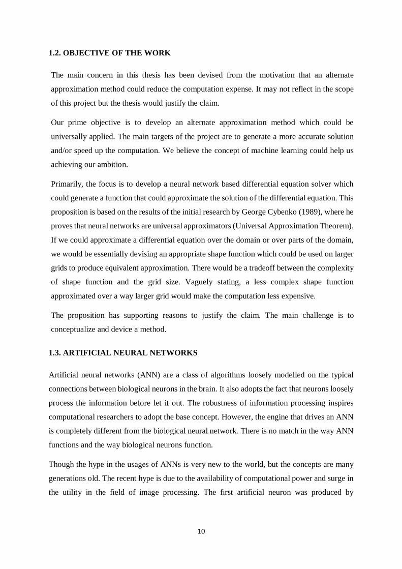
neurophysiologist Warren McCulloch and logician Walter Pits in 1943. The concept of neural

networks was first proposed by Alan Turing in 1948.

A neural network takes single or multiple feed(s) as input. It can produce more than one output

as well. The process that happens in between the input and output is a combination of weighed

linear summation and non-linear activation. Each block that does these processes are called a

neuron (or node). The first task for a neuron is to assign weights to each input and produce a

weighed linear combination of inputs. This generates a single value that represents the total

impact of all the inputs. Most often a bias numerical value is added to it to allow flexibility.

The second task for the neuron is to introduce a non-linearity. The neuron feeds the value

obtained in the last step into a function (called activation function) to get the final output. The

commonly used activation functions are tanh(x), sigmoid(x), ReLU(x), SeLU(x), Heaviside(x)

etc. These non-linear functions allow non-linear scaling of the output. Neural network is a set

of interconnected neurons. A set of parallel neurons is called a hidden layer. If the number of

hidden neurons is more than one, then the network is called deep neural network.

Figure 1.1: Analogy between biological and artificial neuron

Figure 1.2: Deep neural network architecture.

12

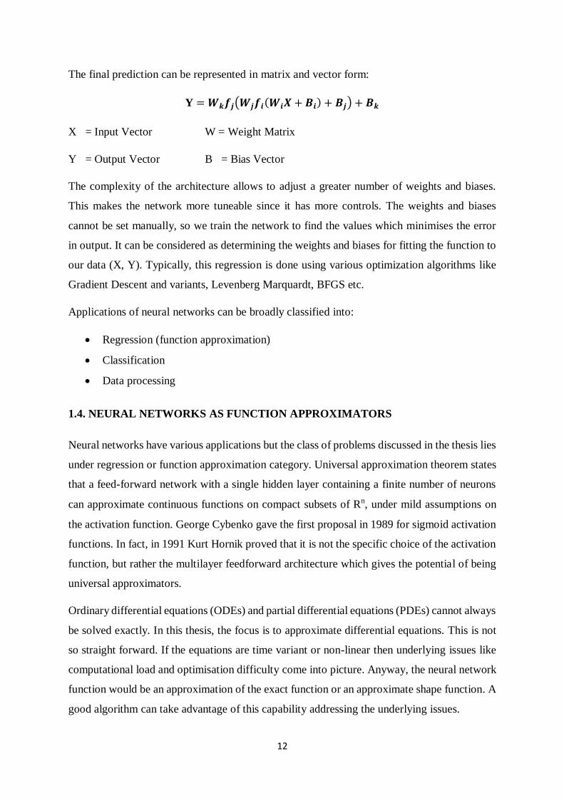
The final prediction can be represented in matrix and vector form:

Y = 𝑾𝒌𝒇𝒋(𝑾𝒋𝒇𝒊(𝑾𝒊𝑿 + 𝑩𝒊) + 𝑩𝒋) + 𝑩𝒌

X = Input Vector W = Weight Matrix

Y = Output Vector B = Bias Vector

The complexity of the architecture allows to adjust a greater number of weights and biases.

This makes the network more tuneable since it has more controls. The weights and biases

cannot be set manually, so we train the network to find the values which minimises the error

in output. It can be considered as determining the weights and biases for fitting the function to

our data (X, Y). Typically, this regression is done using various optimization algorithms like

Gradient Descent and variants, Levenberg Marquardt, BFGS etc.

Applications of neural networks can be broadly classified into:

• Regression (function approximation)

• Classification

• Data processing

1.4. NEURAL NETWORKS AS FUNCTION APPROXIMATORS

Neural networks have various applications but the class of problems discussed in the thesis lies

under regression or function approximation category. Universal approximation theorem states

that a feed-forward network with a single hidden layer containing a finite number of neurons

can approximate continuous functions on compact subsets of Rn, under mild assumptions on

the activation function. George Cybenko gave the first proposal in 1989 for sigmoid activation

functions. In fact, in 1991 Kurt Hornik proved that it is not the specific choice of the activation

function, but rather the multilayer feedforward architecture which gives the potential of being

universal approximators.

Ordinary differential equations (ODEs) and partial differential equations (PDEs) cannot always

be solved exactly. In this thesis, the focus is to approximate differential equations. This is not

so straight forward. If the equations are time variant or non-linear then underlying issues like

computational load and optimisation difficulty come into picture. Anyway, the neural network

function would be an approximation of the exact function or an approximate shape function. A

good algorithm can take advantage of this capability addressing the underlying issues.

13

Three benchmark problems that could targeted are:

1. Steady Advection Diffusion

∁𝒅𝒖

𝒅𝒙= ∈

𝒅𝟐𝒖

𝒅𝒙𝟐

2. Unsteady Linear Advection

𝒅𝒖

𝒅𝒕+ ∁

𝒅𝒖

𝒅𝒙= 𝟎

3. Unsteady Non-Linear Burgers

𝒅𝒖

𝒅𝒕+ 𝒖

𝒅𝒖

𝒅𝒙= ∈

𝒅𝟐𝒖

𝒅𝒙𝟐

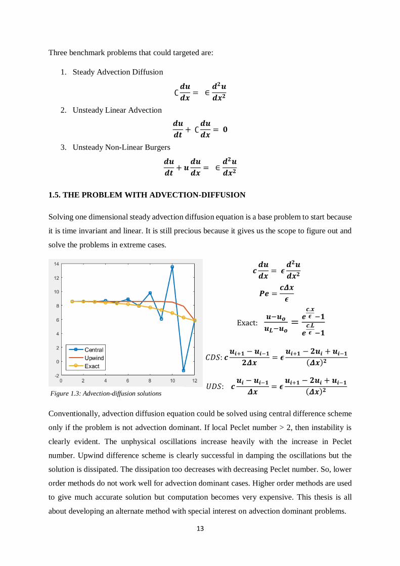
1.5. THE PROBLEM WITH ADVECTION-DIFFUSION

Solving one dimensional steady advection diffusion equation is a base problem to start because

it is time invariant and linear. It is still precious because it gives us the scope to figure out and

solve the problems in extreme cases.

𝒄𝒅𝒖

𝒅𝒙= 𝝐

𝒅𝟐𝒖

𝒅𝒙𝟐

𝑷𝒆 =𝒄𝜟𝒙

𝝐

Exact: 𝒖−𝒖𝒐

𝒖𝑳−𝒖𝒐=

𝒆𝒄.𝒙𝝐 −𝟏

𝒆𝒄.𝑳𝝐 −𝟏

𝐶𝐷𝑆: 𝒄𝒖𝒊+𝟏 − 𝒖𝒊−𝟏

𝟐𝜟𝒙= 𝝐

𝒖𝒊+𝟏 − 𝟐𝒖𝒊 + 𝒖𝒊−𝟏

(𝜟𝒙)𝟐

𝑈𝐷𝑆: 𝒄𝒖𝒊 − 𝒖𝒊−𝟏

𝜟𝒙= 𝝐

𝒖𝒊+𝟏 − 𝟐𝒖𝒊 + 𝒖𝒊−𝟏

(𝜟𝒙)𝟐

Conventionally, advection diffusion equation could be solved using central difference scheme

only if the problem is not advection dominant. If local Peclet number > 2, then instability is

clearly evident. The unphysical oscillations increase heavily with the increase in Peclet

number. Upwind difference scheme is clearly successful in damping the oscillations but the

solution is dissipated. The dissipation too decreases with decreasing Peclet number. So, lower

order methods do not work well for advection dominant cases. Higher order methods are used

to give much accurate solution but computation becomes very expensive. This thesis is all

about developing an alternate method with special interest on advection dominant problems.

Figure 1.3: Advection-diffusion solutions

14

CHAPTER 2

DATA DRIVEN METHODS

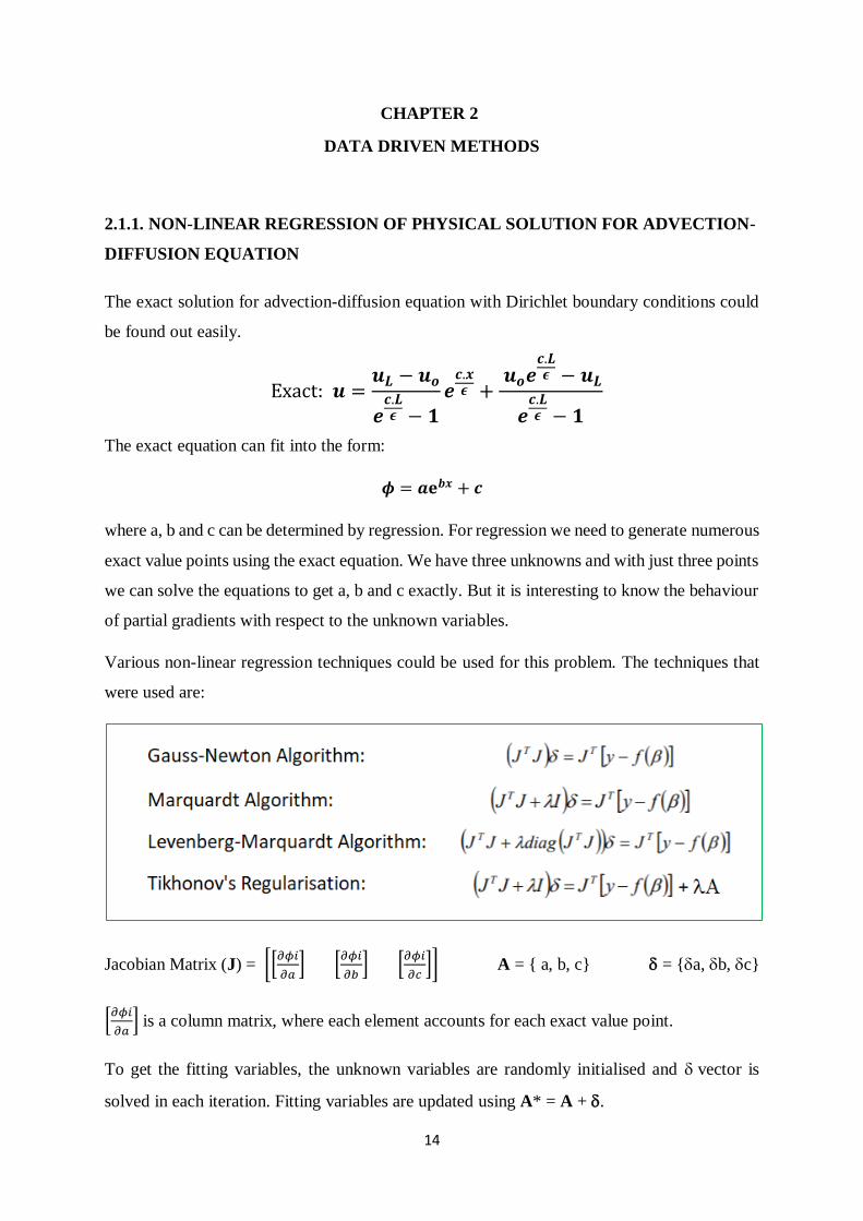
2.1.1. NON-LINEAR REGRESSION OF PHYSICAL SOLUTION FOR ADVECTION-

DIFFUSION EQUATION

The exact solution for advection-diffusion equation with Dirichlet boundary conditions could

be found out easily.

Exact: 𝒖 =𝒖𝑳 − 𝒖𝒐

𝒆𝒄.𝑳𝝐 − 𝟏

𝒆𝒄.𝒙𝝐 +

𝒖𝒐𝒆𝒄.𝑳𝝐 − 𝒖𝑳

𝒆𝒄.𝑳𝝐 − 𝟏

The exact equation can fit into the form:

𝝓 = 𝒂ⅇ𝒃𝒙 + 𝒄

where a, b and c can be determined by regression. For regression we need to generate numerous

exact value points using the exact equation. We have three unknowns and with just three points

we can solve the equations to get a, b and c exactly. But it is interesting to know the behaviour

of partial gradients with respect to the unknown variables.

Various non-linear regression techniques could be used for this problem. The techniques that

were used are:

Jacobian Matrix (J) = [[𝜕𝜙𝑖

𝜕𝑎] [

𝜕𝜙𝑖

𝜕𝑏] [

𝜕𝜙𝑖

𝜕𝑐]] A = { a, b, c} = {a, b, c}

[𝜕𝜙𝑖

𝜕𝑎] is a column matrix, where each element accounts for each exact value point.

To get the fitting variables, the unknown variables are randomly initialised and vector is

solved in each iteration. Fitting variables are updated using A* = A + .

15

2.1.2. OBSERVATIONS

Ideally the fitting should produce very accurate solution but it is not that straight forward.

vector is not always easily solvable. Three types of solutions could be seen:

1. Properly converged

2. Unstable

3. Singular JTJ

Apart from difficulty in solving, solution depends on initialization, boundary conditions and

tuning parameters as well.

Using the Gauss-Newton Algorithm (GNA), for large domain it was clearly evident that the

JTJ matrix became singular. Especially, if 𝝐 < 0.2, then finding the regression becomes

extremely difficult. The small domains over which solution is stable are distributed all over the

R1. However, for negative values 𝝐 of the occurrence of singularity is remarkably rarer. This

is a strange behavior, which comes into frame in further chapters of this thesis as well.

All other techniques mentioned above have regularization parameter () which helps in

conditioning the JTJ matrix to avoid singularity. Even after adjusting the tuning parameter the

regression is unstable for most of the portion of the domain. The Marquardt Algorithm (MA)

and Tikhonov’s Regularization (TR) perform better than the Levenberg-Marquardt Algorithm

(LMA) though LMA is typically assumed to be more robust than the former algorithms. MA,

TR and LMA perform appreciably better than GNA but none of them are robust for our

problem. If 𝝐 < 0.02 none of them are able to produce appreciable regression.

2.2.1. ENHANCEMENT OF SOLUTION FROM CENTRAL DIFFERENCE SCHEME

Central difference scheme (CDS) produces unstable solution for advection dominant problems.

Central differencing is a good approximation for isotropic spread of the property. A map

between CDS solution and exact solution can be easily built using a single layered neural

network since CDS and exact solutions can be easily found out. If a generalized map could be

found out, then it could enhance CDS solution for any advection-diffusion problem. This is the

key advantage of the model.

Let N finite grid points be taken over the test domain. A single layered neural network is trained

with the exact solution for the cases with different 𝝐 and different boundary conditions as

16

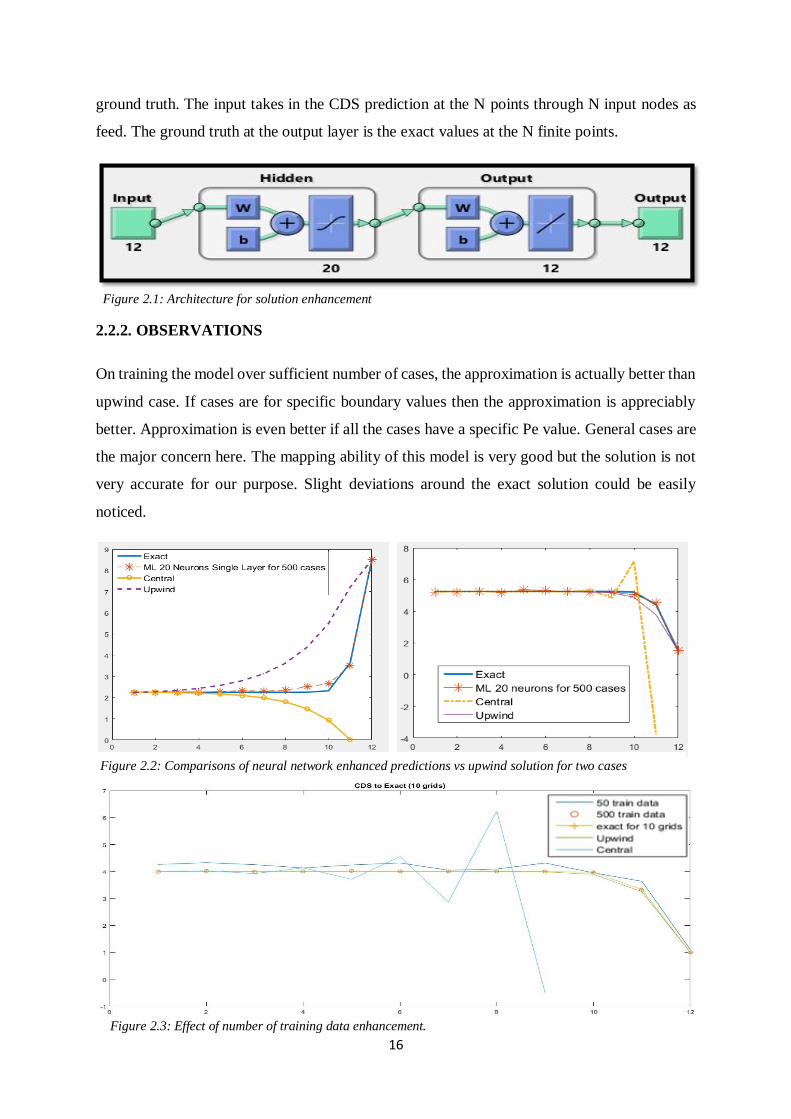
ground truth. The input takes in the CDS prediction at the N points through N input nodes as

feed. The ground truth at the output layer is the exact values at the N finite points.

2.2.2. OBSERVATIONS

On training the model over sufficient number of cases, the approximation is actually better than

upwind case. If cases are for specific boundary values then the approximation is appreciably

better. Approximation is even better if all the cases have a specific Pe value. General cases are

the major concern here. The mapping ability of this model is very good but the solution is not

very accurate for our purpose. Slight deviations around the exact solution could be easily

noticed.

Figure 2.3: Effect of number of training data enhancement.

Figure 2.1: Architecture for solution enhancement

Figure 2.2: Comparisons of neural network enhanced predictions vs upwind solution for two cases

17

The prediction would improve with the increase in the depth of network and increase in the

number of grid points. There are two major limitations of this method. The predictions are

limited to the range of the cases over which the network has been training. It cannot be used to

enhance adverse cases. The second major limitation is inability to enhance the general second

order differential equation (au" + bu' + cu + d = 0). The complexity of the CDS to exact map

increases when generalized. Deeper networks may help on capturing the complexity.

The underlying advantages of this method are ability to predict for very high Pe cases. The

second major advantage is ability to speed up prediction by obtaining coarse CDS solution and

enhancing it to an estimate that we would have obtained from higher resolution solution. In

fact, neural networks could be used to generate higher resolution solution from low resolution

solution. In an experiment, it was observed to be giving better estimate than Richardson’s

extrapolation.

2.3.1. PREDICTION OF ERROR IN CDS SOLUTION

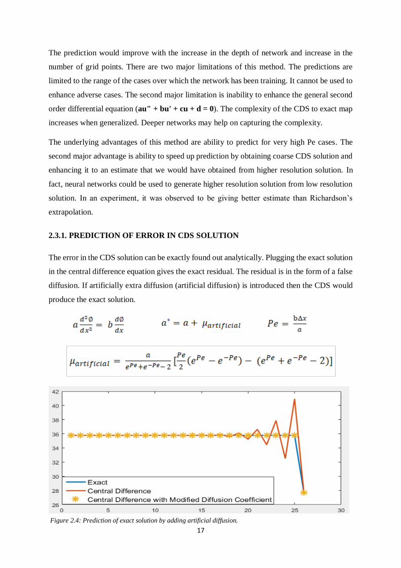
The error in the CDS solution can be exactly found out analytically. Plugging the exact solution

in the central difference equation gives the exact residual. The residual is in the form of a false

diffusion. If artificially extra diffusion (artificial diffusion) is introduced then the CDS would

produce the exact solution.

Figure 2.4: Prediction of exact solution by adding artificial diffusion.

18

artificial is a function of a, b and x. In fact, the function is very similar to the activation function

tanh(x). We designed few architectures which were essentially fed with different combinations

of these three input variables. For instance, (a and Pe), (a, b and Pe), (a, b and x) etc. These

are called different representations for input. We would actually create a function estimator.

This experiment will help us to figure out how easy it is to create a surrogate model to estimate

the artificial diffusion. If such a model works well, it could be used to find the error in

estimation through an extended variant of our model.

2.3.2. OBSERVATIONS

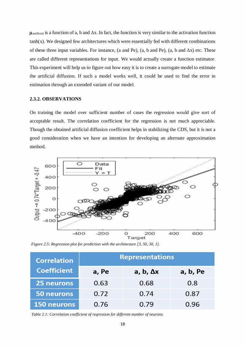
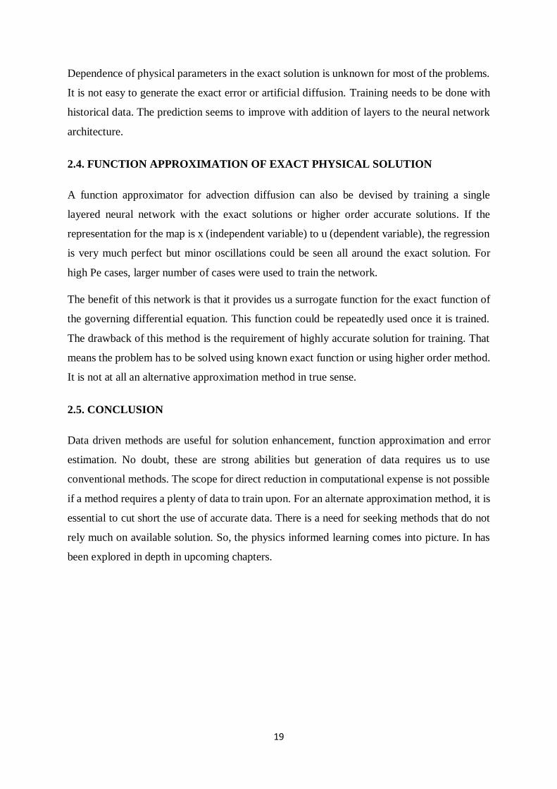
On training the model over sufficient number of cases the regression would give sort of

acceptable result. The correlation coefficient for the regression is not much appreciable.

Though the obtained artificial diffusion coefficient helps in stabilizing the CDS, but it is not a

good consideration when we have an intention for developing an alternate approximation

method.

Figure 2.5: Regression plot for prediction with the architecture [3, 50, 30, 1].

Table 2.1: Correlation coefficient of regression for different number of neurons.

19

Dependence of physical parameters in the exact solution is unknown for most of the problems.

It is not easy to generate the exact error or artificial diffusion. Training needs to be done with

historical data. The prediction seems to improve with addition of layers to the neural network

architecture.

2.4. FUNCTION APPROXIMATION OF EXACT PHYSICAL SOLUTION

A function approximator for advection diffusion can also be devised by training a single

layered neural network with the exact solutions or higher order accurate solutions. If the

representation for the map is x (independent variable) to u (dependent variable), the regression

is very much perfect but minor oscillations could be seen all around the exact solution. For

high Pe cases, larger number of cases were used to train the network.

The benefit of this network is that it provides us a surrogate function for the exact function of

the governing differential equation. This function could be repeatedly used once it is trained.

The drawback of this method is the requirement of highly accurate solution for training. That

means the problem has to be solved using known exact function or using higher order method.

It is not at all an alternative approximation method in true sense.

2.5. CONCLUSION

Data driven methods are useful for solution enhancement, function approximation and error

estimation. No doubt, these are strong abilities but generation of data requires us to use

conventional methods. The scope for direct reduction in computational expense is not possible

if a method requires a plenty of data to train upon. For an alternate approximation method, it is

essential to cut short the use of accurate data. There is a need for seeking methods that do not

rely much on available solution. So, the physics informed learning comes into picture. In has

been explored in depth in upcoming chapters.

20

CHAPTER 3

PHYSICS INFORMED LEARNING

3.1. PHYSICS INFORMED NEURAL NETWORK FOR SOLVING ODE AND PDE

The usual neural networks are based on data that are fed. The model just tries to fit into the

data. There is no need for understanding the physics behind the problem to train a neural

network. This is the reason why there are small noise like oscillations around the exact solution.

It is essential to make the neural network function learn the physics of the problem.

Solving a regression problem is an optimization problem. The easiest way to introduce the

physics into the problem is to somehow introduce it in the optimization objective. I.E. Lagaris

et. al. in 1997 suggested a way to do so. Solving a differential equation is treated as an

optimization problem over a neural network function and not really treated as a training

problem. The beauty of this algorithm is that, it does not require any data to get the required

neural network trained. Only the values of independent variables are fed for training. The initial

and boundary conditions are also required to be fed into the optimization objective.

3.2.1. LAGARIS’ ALGORITHM

A function approximator for any differential equation is proposed to be build. It should take in

the values of independent variables like x, y, z etc. The method suggested by Lagaris et. al. in

1997 uses a single layered neural network with sigmoid activation function to satisfy the

differential equation. The residual after plugging in the neural network function (𝑁(𝑥𝑖⃗⃗⃗ , 𝑝 )) is a

good measure of error. To inform the boundary constraints a trial function (𝜓) is proposed to

be plugged in, instead of plugging in the neural network function directly. The trial function is

a mathematically transformed function of the neural network function that satisfies the

constraints exactly. A properly trained network would produce extremely low residual.

Minimization of this residual (Gi) is a beautiful way to impose physics into the neural network.

So, the least squared sum of residual over the grid points is the loss function. The points over

which the network is trained are called collocation points.

𝐿 = 𝑚𝑖𝑛𝑝 ∑𝐺2(𝑥𝑖⃗⃗ ⃗, 𝜓(𝑥𝑖⃗⃗ ⃗, 𝑝 ), 𝛻𝜓(𝑥𝑖⃗⃗ ⃗, 𝑝 ), 𝛻2𝜓(𝑥𝑖⃗⃗ ⃗, 𝑝 ))

𝜓(𝑥 , 𝑝 ) = 𝐴(𝑥 ) + 𝐹(𝑥 ,𝑁(𝑥 , 𝑝 ))

21

The parameters (�⃗⃗� ) contains the weights and biases for the network. The gradients are

calculated using the AutoGrad technique, easily available on TensorFlow now a days.

3.2.2. LAGARIS’ IMPLEMENTATION OF ADVECTION DIFFUSION

The base problem of steady one-dimensional advection diffusion equation is solved under

Dirichlet boundary conditions {u(0) = 𝑢𝐿, u(1) = 𝑢𝑅}. So, the trial function and the loss

function are:

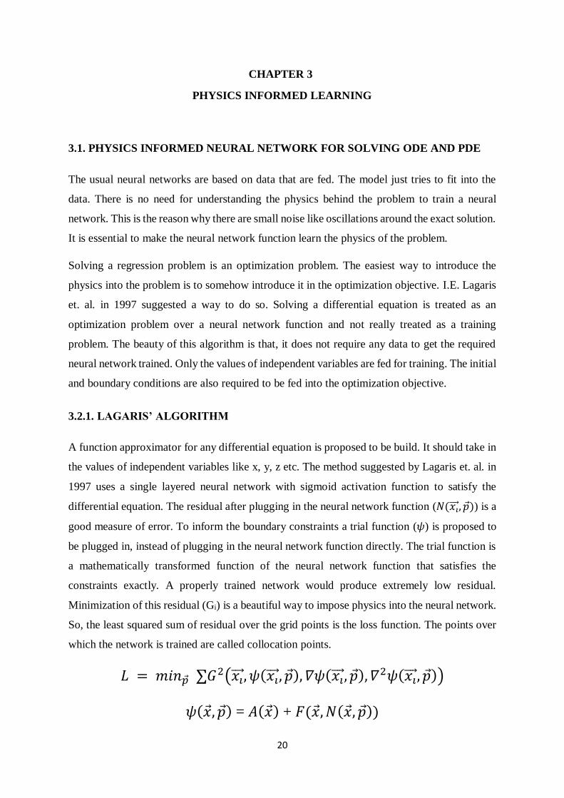
𝜓(𝑥, 𝑝 ) = (1 − 𝑥)𝑢𝐿 + 𝑥𝑢𝑅 + 𝑥(1 − 𝑥)𝑁(𝑥, 𝑝 )

L(𝑝 ) = ∑[𝜖𝜕2𝜓(𝑥,𝑝 )

𝜕𝑥2−

𝜕𝜓(𝑥,𝑝 )

𝜕𝑥]2

Regular optimizers like gradient descent could be used as regular neural network. It works

really well for 𝜖 > 0.6 but with decrease in the value the estimation deviates from the exact

solution. The boundaries are always intact since we have forced them in the trial function. If 𝜖

is very low like 0.1 or less then the model fails and it is unable to converge. So, keeping the

boundaries in place makes it difficult for optimization. This is a serious problem and there will

be multiple evidences in further chapters as well. Not much improvement could be noticed with

increased number of neurons in the hidden layer. Since, there are no much other parameter

which could be controlled, it proves the incapability of the method to solve such problems.

Lagaris’ method can be used for a wide class of differential equations but it cannot provide

solution for extreme cases, like in the case advective dominance. A strong limitation of this

𝜖 = 0.3 𝜖 = 0.7

Figure 3.1: Comparison of prediction using Lagaris’ concept for 𝜖 = 0.3 and 0.7.

{blue curve represents the exact solution while orange curve is the prediction} The curves on the right seems to be overlapping on each other.

22

approach is that the trial function needs to defined appropriately for each problem. This makes

the model less generalizable. The other major limitation is the inability to solve time variant

problems. Solving initial value problems using this method seems to be very inefficient.

3.3.1. PHYSICS INFORMED DEEP LEARNING BY MAZIAR RAISSI ET.AL.

Maziar Raissi et. al., in 2017, came up with a development over the method proposed by

Lagaris et. al. The proposed method addresses the limitations of Lagaris’ method that has been

mentioned at the end of the last segment. The core improvements are:

1. Additional loss terms are computed as mean squared error at boundaries to satisfy the

boundary conditions. The makes the method generalizable to almost all the classes of

ODEs and PDEs. Numerous boundary conditions could be enforced as additional mean

squared error loss terms. There is no need for altering the trial function, the neural

network itself can do the job of trial function.

2. The second benefit of using additional loss term for boundary constraints is allowing

relaxation at boundaries during the course of optimization makes the convergence

easier and simpler. Though there will be slight deviation from boundary values but as

the optimization converges the values start matching the exact values very accurately.

3. Initial conditions could be imposed by addition of extra loss terms as mean of squared

errors of the initial value data, very much like boundary constraints. This improvement

makes it usable to solve time variant problems like advection and burgers.

4. The architecture in this model allows deeper layers, which makes it possible to solve

complex and non-linear functions.

The formulations for trail function (𝜓), loss function (L), collocation loss(Lf), boundary

constraint loss (Lb) and initial constraint loss (Li) are:

𝜓(𝑥, 𝑡, 𝑝 ) = Neural 𝑁𝑒𝑡𝑤𝑜𝑟𝑘(𝑥, 𝑡, 𝑝 )

Lf(𝑝 ) = 1

𝑁𝑓∑[ 𝑓𝐷𝐸 (

𝜕𝑛𝜓(𝑥,𝑡,𝑝 )

𝜕𝑥𝑛 , . . ,𝜕2𝜓(𝑥,𝑡,𝑝 )

𝜕𝑥2 ,𝜕𝜓(𝑥,𝑡,𝑝 )

𝜕𝑥)]

2

Lb(𝑝 ) = 1

𝑁𝑏∑[𝜓(𝑥𝑏

𝑘, 𝑡, 𝑝 ) − 𝜓𝑏𝑘]

2

Li(𝑝 ) = 1

𝑁𝑖∑[𝜓(𝑥𝑖

𝑘, 𝑡, 𝑝 ) − 𝜓𝑖𝑘]

2

23

L(𝑝 ) = Lf(𝑝 ) + Lb(𝑝 ) + Li(𝑝 )

Nf, Nb and Ni are numbers of collocation points, boundary points and initial points respectively.

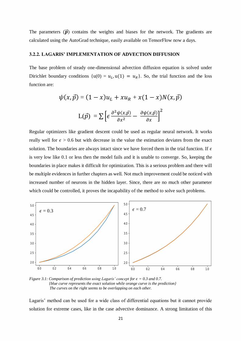
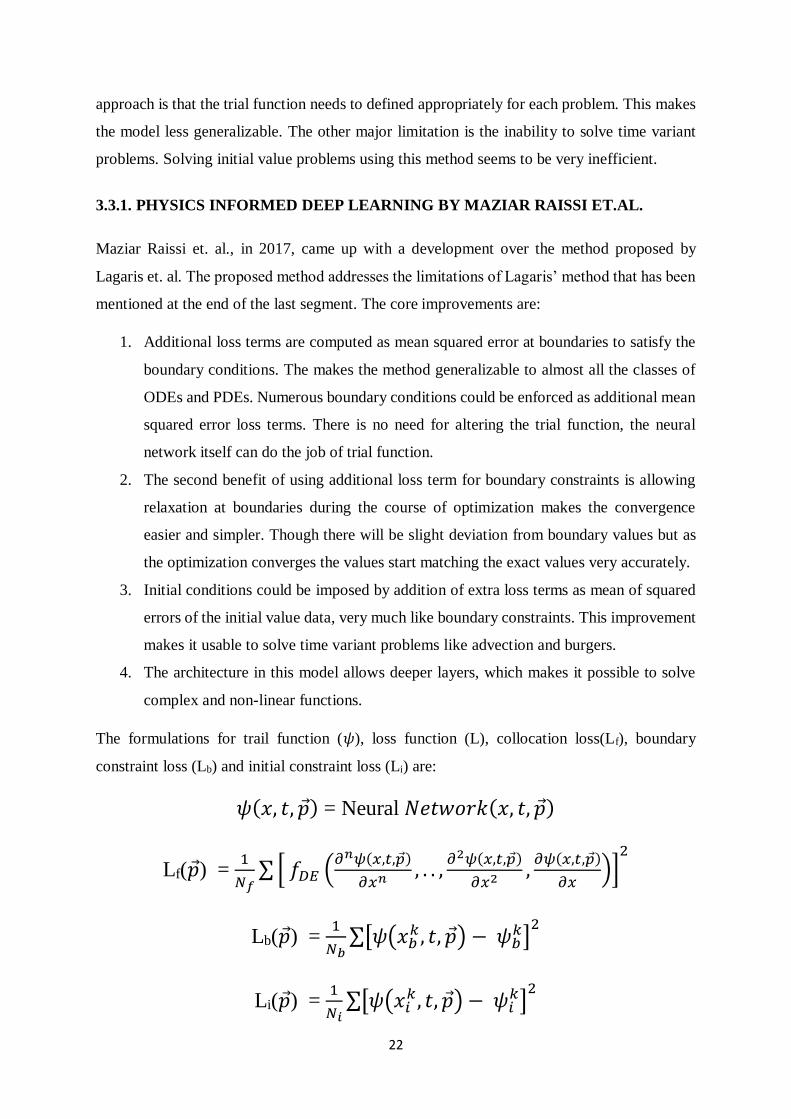
3.3.2. PINN IMPLEMENTATION FOR ADVECTION DIFFUSION

For advection diffusion,

𝑓𝐷𝐸 = 𝜖𝜕2𝜓(𝑥, 𝑡, 𝑝 )

𝜕𝑥2−

𝜕𝜓(𝑥, 𝑡, 𝑝 )

𝜕𝑥

PINN’s implementation makes it possible to solve problems for 𝜖 > 0.14. This is a remarkable

improvement, since the previous method could produce solution for 𝜖 > 0.6. Practically

speaking, 𝜖 > 0.1 is not a sufficient range.

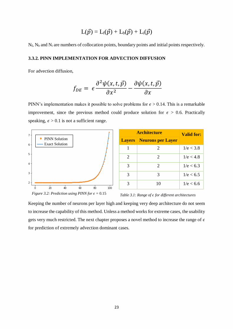
Architecture Valid for:

Layers Neurons per Layer

1 2 1/e < 3.8

2 2 1/e < 4.8

3 2 1/e < 6.3

3 3 1/e < 6.5

3 10 1/e < 6.6

Keeping the number of neurons per layer high and keeping very deep architecture do not seem

to increase the capability of this method. Unless a method works for extreme cases, the usability

gets very much restricted. The next chapter proposes a novel method to increase the range of 𝜖

for prediction of extremely advection dominant cases.

Figure 3.2: Prediction using PINN for 𝜖 = 0.15

PINN Solution

Exact Solution

Table 3.1: Range of 𝜖 for different architectures

24

CHAPTER 4

DISTRIBUTED PHYSICS INFORMED NEURAL NETWORK (DPINN)

4.1. INTRODUCTION

The available methods cannot provide solution for 𝜖 < 0.1. The optimization becomes very

tough for the method because for extremely low 𝜖 the architecture could not capture the sharp

gradient that appears quite sudden in the course of domain. To reduce the burden over a

network it has been decided to go for a series of small networks. The idea is to fit the equation

piece-wise. It is analogous to piece wise curve fitting. Each piece is essentially a sub-domain

and there will be a network for each sub-domain to approximate for the sub-domain.

4.2. DATA DRIVEN DISTRIBUTED NEURAL NETWORK

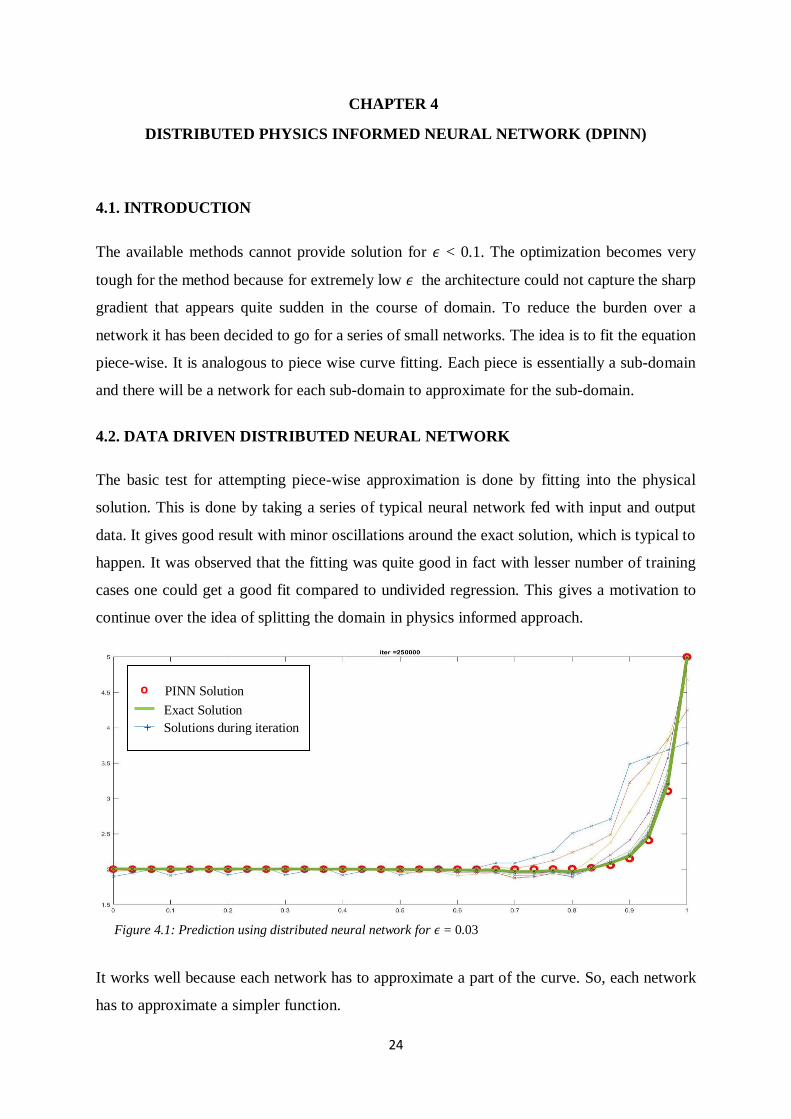
The basic test for attempting piece-wise approximation is done by fitting into the physical

solution. This is done by taking a series of typical neural network fed with input and output

data. It gives good result with minor oscillations around the exact solution, which is typical to

happen. It was observed that the fitting was quite good in fact with lesser number of training

cases one could get a good fit compared to undivided regression. This gives a motivation to

continue over the idea of splitting the domain in physics informed approach.

It works well because each network has to approximate a part of the curve. So, each network

has to approximate a simpler function.

Figure 4.1: Prediction using distributed neural network for 𝜖 = 0.03

o PINN Solution

Exact Solution

+ Solutions during iteration

25

4.3. DISTRIBUTED PHYSICS INFORMED NEURAL NETWORK (DPINN)

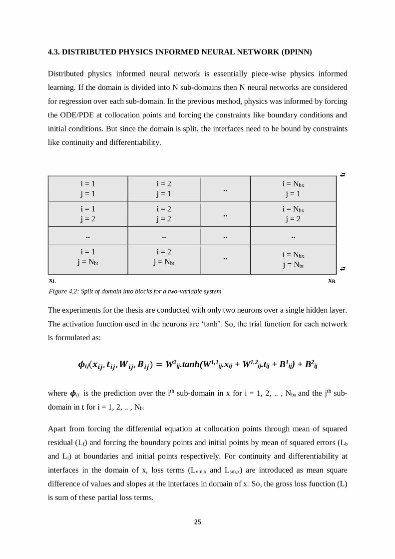
Distributed physics informed neural network is essentially piece-wise physics informed

learning. If the domain is divided into N sub-domains then N neural networks are considered

for regression over each sub-domain. In the previous method, physics was informed by forcing

the ODE/PDE at collocation points and forcing the constraints like boundary conditions and

initial conditions. But since the domain is split, the interfaces need to be bound by constraints

like continuity and differentiability.

i = 1

j = 1

i = 2

j = 1 ..

i = Nbx

j = 1

i = 1

j = 2

i = 2

j = 2 ..

i = Nbx

j = 2

.. .. .. ..

i = 1

j = Nbt

i = 2

j = Nbt .. i = Nbx

j = Nbt

The experiments for the thesis are conducted with only two neurons over a single hidden layer.

The activation function used in the neurons are ‘tanh’. So, the trial function for each network

is formulated as:

𝝓ij(𝒙𝒊𝒋, 𝒕𝒊𝒋,𝑾𝒊𝒋, 𝑩𝒊𝒋) = W2ij.tanh(W1,1

ij.xij + W1,2ij.tij + B1

ij) + B2ij

where 𝝓ij is the prediction over the ith sub-domain in x for i = 1, 2, .. , Nbx and the jth sub-

domain in t for i = 1, 2, .. , Nbt

Apart from forcing the differential equation at collocation points through mean of squared

residual (Lf) and forcing the boundary points and initial points by mean of squared errors (Lb

and Li) at boundaries and initial points respectively. For continuity and differentiability at

interfaces in the domain of x, loss terms (Lvm,x and Lsm,x) are introduced as mean square

difference of values and slopes at the interfaces in domain of x. So, the gross loss function (L)

is sum of these partial loss terms.

xL xR

t i

tf

Figure 4.2: Split of domain into blocks for a two-variable system

26

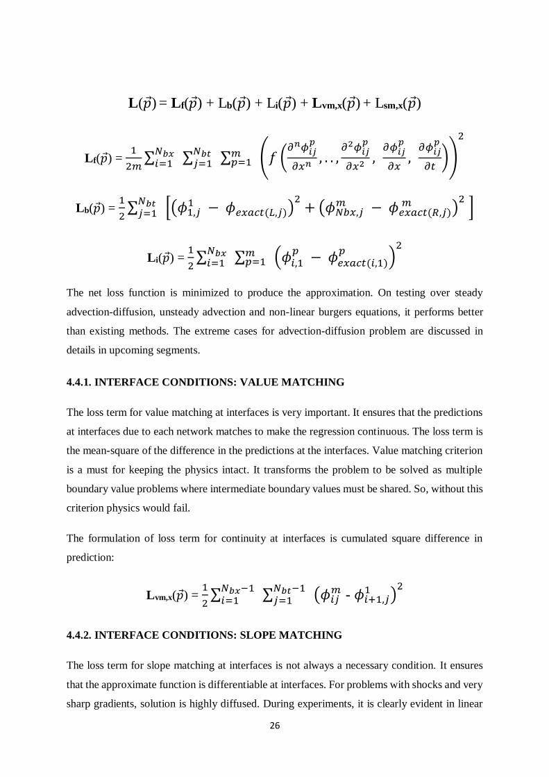
L(𝑝 ) = Lf(𝑝 ) + Lb(𝑝 ) + Li(𝑝 ) + Lvm,x(𝑝 ) + Lsm,x(𝑝 )

Lf(𝑝 ) = 1

2𝑚∑

𝑁𝑏𝑥𝑖=1 ∑

𝑁𝑏𝑡𝑗=1 ∑ 𝑚

𝑝=1 (𝑓 (𝜕𝑛𝜙𝑖𝑗

𝑝

𝜕𝑥𝑛 , . . ,𝜕2𝜙𝑖𝑗

𝑝

𝜕𝑥2 ,𝜕𝜙𝑖𝑗

𝑝

𝜕𝑥,

𝜕𝜙𝑖𝑗𝑝

𝜕𝑡))

2

Lb(𝑝 ) = 1

2∑

𝑁𝑏𝑡𝑗=1 [(𝜙1,𝑗

1 − 𝜙𝑒𝑥𝑎𝑐𝑡(𝐿,𝑗) )

2+ (𝜙𝑁𝑏𝑥,𝑗

𝑚 − 𝜙𝑒𝑥𝑎𝑐𝑡(𝑅,𝑗) 𝑚 )

2 ]

Li(𝑝 ) = 1

2∑

𝑁𝑏𝑥𝑖=1 ∑ 𝑚

𝑝=1 (𝜙𝑖,1𝑝

− 𝜙𝑒𝑥𝑎𝑐𝑡(𝑖,1)𝑝

)2

The net loss function is minimized to produce the approximation. On testing over steady

advection-diffusion, unsteady advection and non-linear burgers equations, it performs better

than existing methods. The extreme cases for advection-diffusion problem are discussed in

details in upcoming segments.

4.4.1. INTERFACE CONDITIONS: VALUE MATCHING

The loss term for value matching at interfaces is very important. It ensures that the predictions

at interfaces due to each network matches to make the regression continuous. The loss term is

the mean-square of the difference in the predictions at the interfaces. Value matching criterion

is a must for keeping the physics intact. It transforms the problem to be solved as multiple

boundary value problems where intermediate boundary values must be shared. So, without this

criterion physics would fail.

The formulation of loss term for continuity at interfaces is cumulated square difference in

prediction:

Lvm,x(𝑝 ) = 1

2∑

𝑁𝑏𝑥−1𝑖=1 ∑

𝑁𝑏𝑡−1𝑗=1 (𝜙𝑖𝑗

𝑚 - 𝜙𝑖+1,𝑗1 )

2

4.4.2. INTERFACE CONDITIONS: SLOPE MATCHING

The loss term for slope matching at interfaces is not always a necessary condition. It ensures

that the approximate function is differentiable at interfaces. For problems with shocks and very

sharp gradients, solution is highly diffused. During experiments, it is clearly evident in linear

27

unsteady advection of heaviside function or square pulse. While for continuous and

differentiable functions, using this additional loss term smoothens the optimization. Even using

slope matching loss term helps in equations with diffusion terms like advection-diffusion and

burgers.

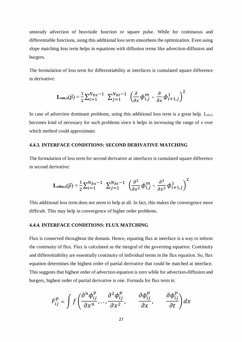
The formulation of loss term for differentiability at interfaces is cumulated square difference

in derivative:

Lsm,x(𝑝 ) = 1

2∑

𝑁𝑏𝑥−1𝑖=1 ∑

𝑁𝑏𝑡−1𝑗=1 (

𝜕

𝜕𝑥𝜙𝑖,𝑗

𝑚 - 𝜕

𝜕𝑥𝜙𝑖+1,𝑗

1 )2

In case of advection dominant problems, using this additional loss term is a great help. Lsm,x

becomes kind of necessary for such problems since it helps in increasing the range of 𝜖 over

which method could approximate.

4.4.3. INTERFACE CONDITIONS: SECOND DERIVATIVE MATCHING

The formulation of loss term for second derivative at interfaces is cumulated square difference

in second derivative:

Lsdm,x(𝑝 ) = 1

2∑

𝑁𝑏𝑥−1𝑖=1 ∑

𝑁𝑏𝑡−1𝑗=1 (

𝜕2

𝜕𝑥2𝜙𝑖,𝑗

𝑚 - 𝜕2

𝜕𝑥2𝜙𝑖+1,𝑗

1 )2

This additional loss term does not seem to help at all. In fact, this makes the convergence more

difficult. This may help in convergence of higher order problems.

4.4.4. INTERFACE CONDITIONS: FLUX MATCHING

Flux is conserved throughout the domain. Hence, equating flux at interface is a way to inform

the continuity of flux. Flux is calculated as the integral of the governing equation. Continuity

and differentiability are essentially continuity of individual terms in the flux equation. So, flux

equation determines the highest order of partial derivative that could be matched at interface.

This suggests that highest order of advection equation is zero while for advection-diffusion and

burgers, highest order of partial derivative is one. Formula for flux term is:

𝐹𝑖𝑗𝑝

= ∫𝑓(𝜕𝑛𝜙𝑖𝑗

𝑝

𝜕𝑥𝑛, . . ,

𝜕2𝜙𝑖𝑗𝑝

𝜕𝑥2,

𝜕𝜙𝑖𝑗𝑝

𝜕𝑥,

𝜕𝜙𝑖𝑗𝑝

𝜕𝑡)𝑑𝑥

28

The formulation of loss term for flux continuity at interfaces is cumulated square difference in

flux:

Lfm,x(𝑝 ) = 1

2∑

𝑁𝑏𝑥−1𝑖=1 ∑

𝑁𝑏𝑡−1𝑗=1 (𝐹𝑖𝑗

𝑚 - 𝐹𝑖+1,𝑗1 )

2

This additional loss term has nearly similar effect of slope matching at interfaces. Slope

matching and flux matching could be used interchangeably. Keeping or discarding this loss

term does not seem to make significant change in convergence.

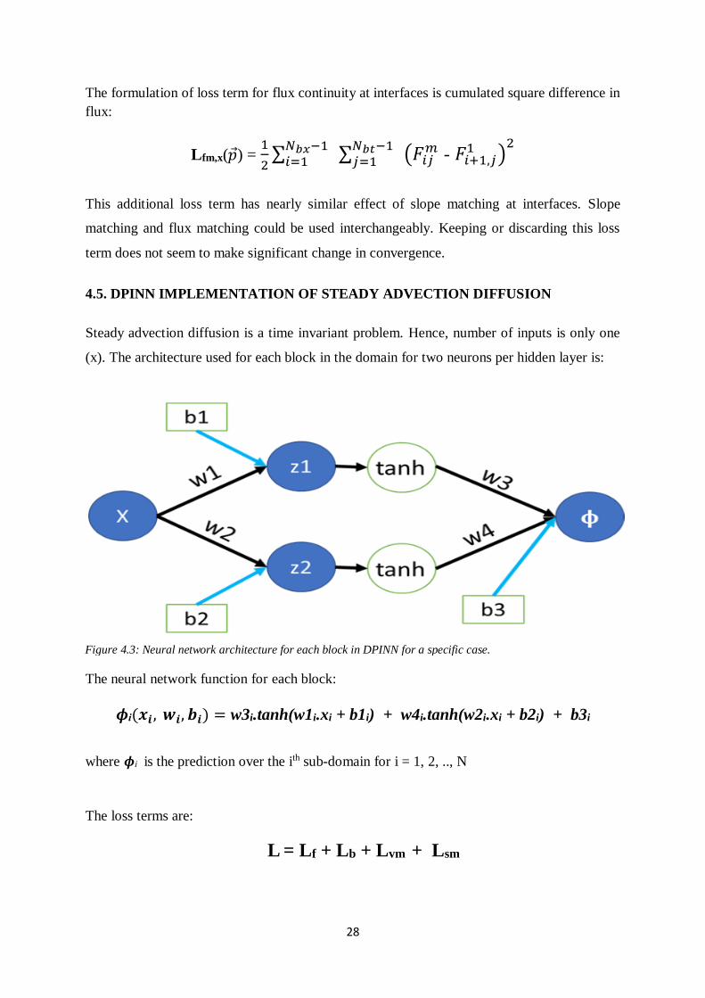
4.5. DPINN IMPLEMENTATION OF STEADY ADVECTION DIFFUSION

Steady advection diffusion is a time invariant problem. Hence, number of inputs is only one

(x). The architecture used for each block in the domain for two neurons per hidden layer is:

The neural network function for each block:

𝝓i(𝒙𝒊, 𝒘𝒊, 𝒃𝒊) = w3i.tanh(w1i.xi + b1i) + w4i.tanh(w2i.xi + b2i) + b3i

where 𝝓i is the prediction over the ith sub-domain for i = 1, 2, .., N

The loss terms are:

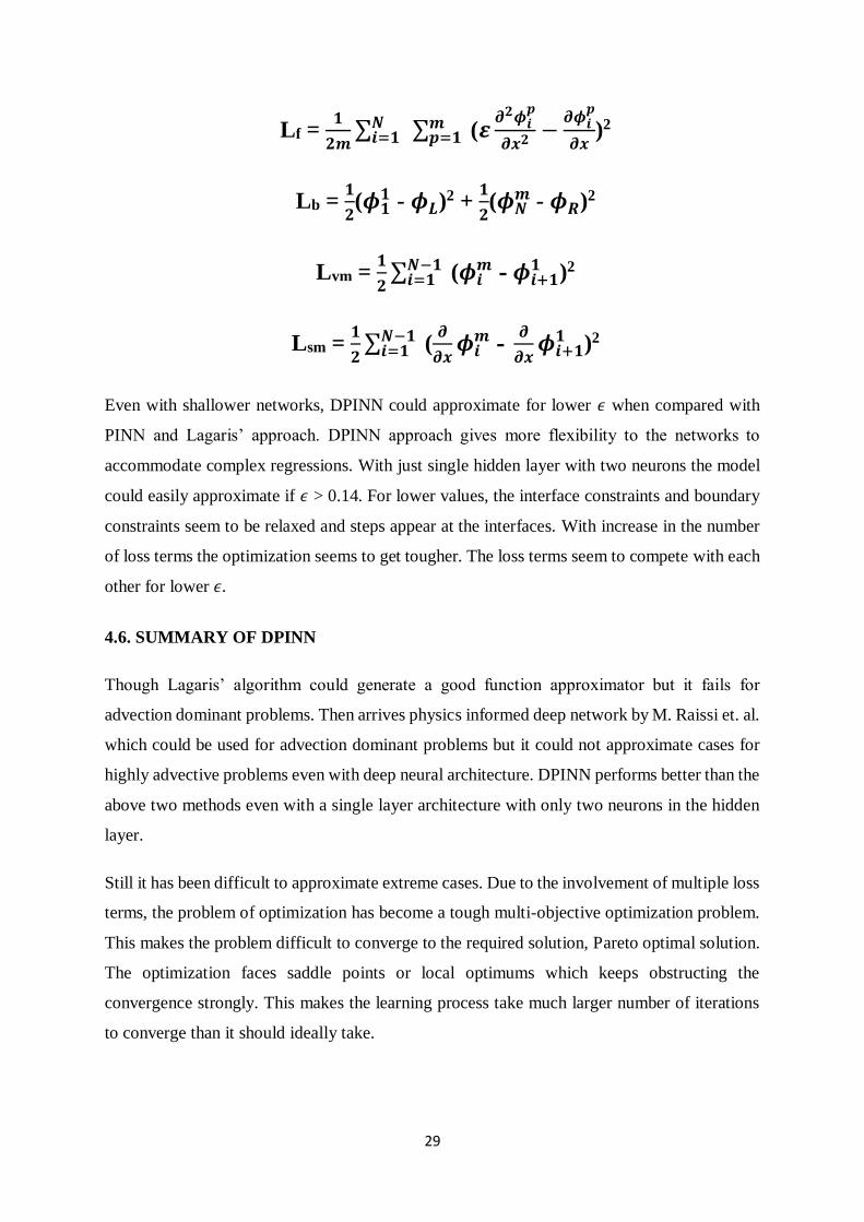
L = Lf + Lb + Lvm + Lsm

Figure 4.3: Neural network architecture for each block in DPINN for a specific case.

29

Lf = 𝟏

𝟐𝒎∑ 𝑵

𝒊=𝟏 ∑ 𝒎𝒑=𝟏 (𝜺

𝝏𝟐𝝓𝒊𝒑

𝝏𝒙𝟐 −𝝏𝝓𝒊

𝒑

𝝏𝒙)2

Lb = 𝟏

𝟐(𝝓𝟏

𝟏 - 𝝓𝑳 )2 +

𝟏

𝟐(𝝓𝑵

𝒎 - 𝝓𝑹 )2

Lvm = 𝟏

𝟐∑ 𝑵−𝟏

𝒊=𝟏 (𝝓𝒊𝒎 - 𝝓𝒊+𝟏

𝟏 )2

Lsm = 𝟏

𝟐∑ 𝑵−𝟏

𝒊=𝟏 (𝝏

𝝏𝒙𝝓𝒊

𝒎 - 𝝏

𝝏𝒙𝝓𝒊+𝟏

𝟏 )2

Even with shallower networks, DPINN could approximate for lower 𝜖 when compared with

PINN and Lagaris’ approach. DPINN approach gives more flexibility to the networks to

accommodate complex regressions. With just single hidden layer with two neurons the model

could easily approximate if 𝜖 > 0.14. For lower values, the interface constraints and boundary

constraints seem to be relaxed and steps appear at the interfaces. With increase in the number

of loss terms the optimization seems to get tougher. The loss terms seem to compete with each

other for lower 𝜖.

4.6. SUMMARY OF DPINN

Though Lagaris’ algorithm could generate a good function approximator but it fails for

advection dominant problems. Then arrives physics informed deep network by M. Raissi et. al.

which could be used for advection dominant problems but it could not approximate cases for

highly advective problems even with deep neural architecture. DPINN performs better than the

above two methods even with a single layer architecture with only two neurons in the hidden

layer.

Still it has been difficult to approximate extreme cases. Due to the involvement of multiple loss

terms, the problem of optimization has become a tough multi-objective optimization problem.

This makes the problem difficult to converge to the required solution, Pareto optimal solution.

The optimization faces saddle points or local optimums which keeps obstructing the

convergence strongly. This makes the learning process take much larger number of iterations

to converge than it should ideally take.

30

CHAPTER 5

EXPERIMENTS TO ENHANCE DPINN

5.1. INTRODUCTION

In this chapter various reports of various trial and experiments conducted to enhance the

DPINN algorithm are recorded topic wise.

5.2. RANDOM COLLOCATION POINTS FOR FORCING THE EQUATION

Overfitting is evident in the vicinity of shocks and sharp gradients. It could be seen in around

the edges square pulse in linear advection. Initially, uniformly domain points were fed for

forcing the differential equation at only specific points as a result the behaviour of the function

at neighbouring points could not be captured.

New set of random points are generated within each block before each iteration of optimization.

Considering random points within blocks helps in protecting the network from over fitting. It

also helps in speeding up the convergence. The predictions at edges becomes neater. It should

be noted that, forcing the differential equation at end points perform better than otherwise.

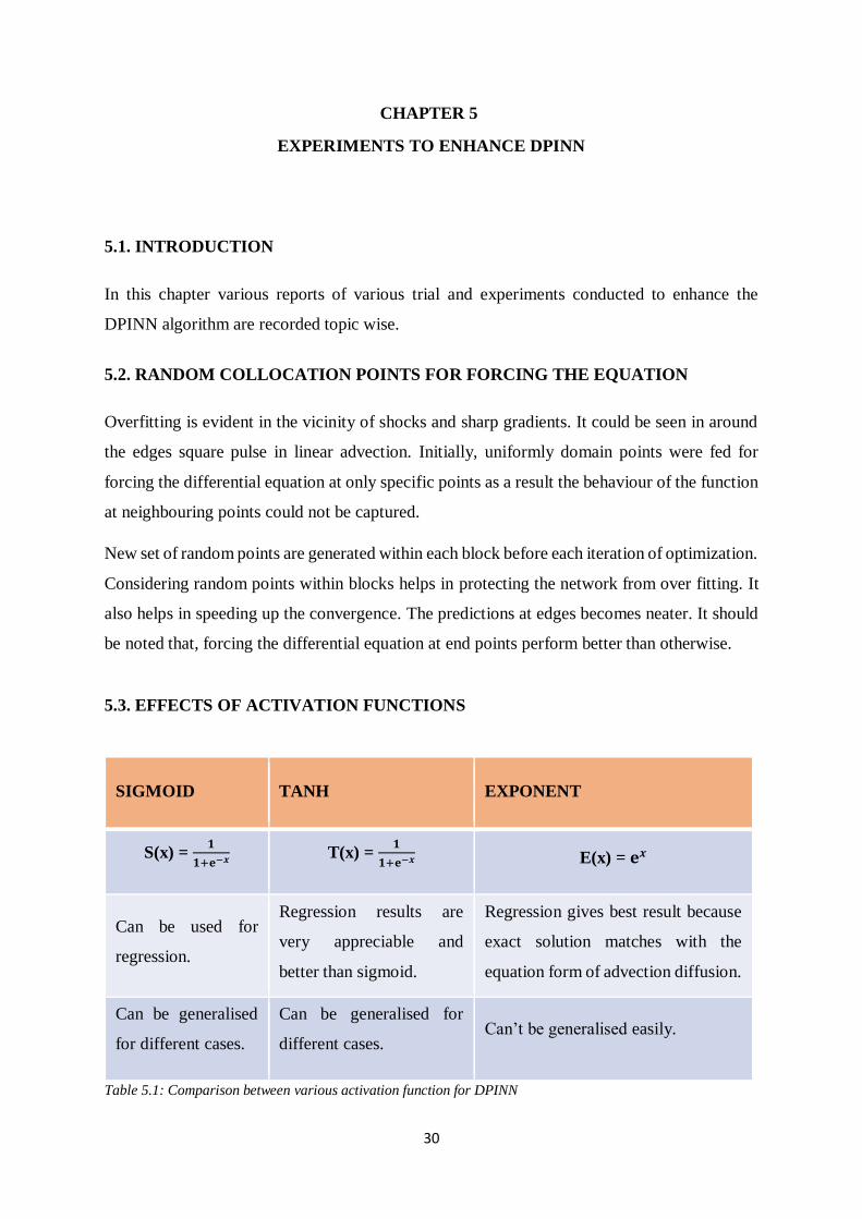
5.3. EFFECTS OF ACTIVATION FUNCTIONS

Table 5.1: Comparison between various activation function for DPINN

SIGMOID TANH EXPONENT

S(x) = 𝟏

𝟏+ⅇ−𝒙 T(x) = 𝟏

𝟏+ⅇ−𝒙 E(x) = ⅇ𝒙

Can be used for

regression.

Regression results are

very appreciable and

better than sigmoid.

Regression gives best result because

exact solution matches with the

equation form of advection diffusion.

Can be generalised

for different cases.

Can be generalised for

different cases. Can’t be generalised easily.

31

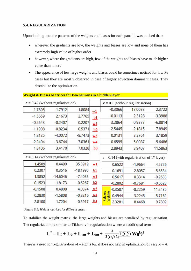
5.4. REGULARIZATION

Upon looking into the patterns of the weights and biases for each panel it was noticed that:

• wherever the gradients are low, the weights and biases are low and none of them has

extremely high value of higher order

• however, where the gradients are high, few of the weights and biases have much higher

value than others

• The appearance of few large weights and biases could be sometimes noticed for low Pe

cases but they are mostly observed in case of highly advection dominant cases. They

destabilize the optimization.

Weight & Biases Matrices for two neurons in a hidden layer .

To stabilize the weight matrix, the large weights and biases are penalized by regularization.

The regularization is similar to Tikhonov’s regularization where an additional term

L* = Lf + Lb + Lvm + Lsm +

𝝀

𝟐(𝒊∗𝒋∗𝒌)∑∑∑(Wij

k)2

There is a need for regularization of weights but it does not help in optimization of very low 𝝐.

𝝐 = 0.42 (without regularisation)

𝝐 = 0.1 (without regularisation)

𝝐 = 0.14 (without regularisation) 𝝐 = 0.14 (with regularization of 1st layer)

w1

b1

w2

b2

w3

w4

b3

w1

b1

w2

b2

w3

w4

b3

Rel

axed

W

eigh

ts

Figure 5.1: Weight matrices for different cases.

32

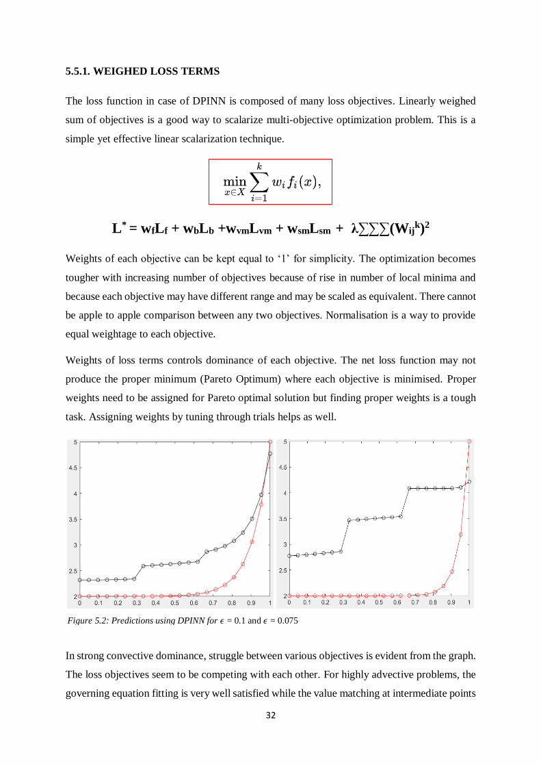
5.5.1. WEIGHED LOSS TERMS

The loss function in case of DPINN is composed of many loss objectives. Linearly weighed

sum of objectives is a good way to scalarize multi-objective optimization problem. This is a

simple yet effective linear scalarization technique.

L* = wfLf + wbLb +wvmLvm + wsmLsm + λ∑∑∑(Wij

k)2

Weights of each objective can be kept equal to ‘1’ for simplicity. The optimization becomes

tougher with increasing number of objectives because of rise in number of local minima and

because each objective may have different range and may be scaled as equivalent. There cannot

be apple to apple comparison between any two objectives. Normalisation is a way to provide

equal weightage to each objective.

Weights of loss terms controls dominance of each objective. The net loss function may not

produce the proper minimum (Pareto Optimum) where each objective is minimised. Proper

weights need to be assigned for Pareto optimal solution but finding proper weights is a tough

task. Assigning weights by tuning through trials helps as well.

In strong convective dominance, struggle between various objectives is evident from the graph.

The loss objectives seem to be competing with each other. For highly advective problems, the

governing equation fitting is very well satisfied while the value matching at intermediate points

Figure 5.2: Predictions using DPINN for 𝜖 = 0.1 and 𝜖 = 0.075

33

and boundary points matching fails heavily. So, penalizing the fitting loss term by dividing the

loss term by 10-50 helps. Similarly, prioritizing the boundary point loss and value matching at

intermediate points by multiplying the loss term by 10-50 helps.

Error due to slope at intermediate points is not much. Changing the weight for that case does

not seem to respond to well to direct toward the actual solution. Somehow, it is subtly stable

weight equals to 1.

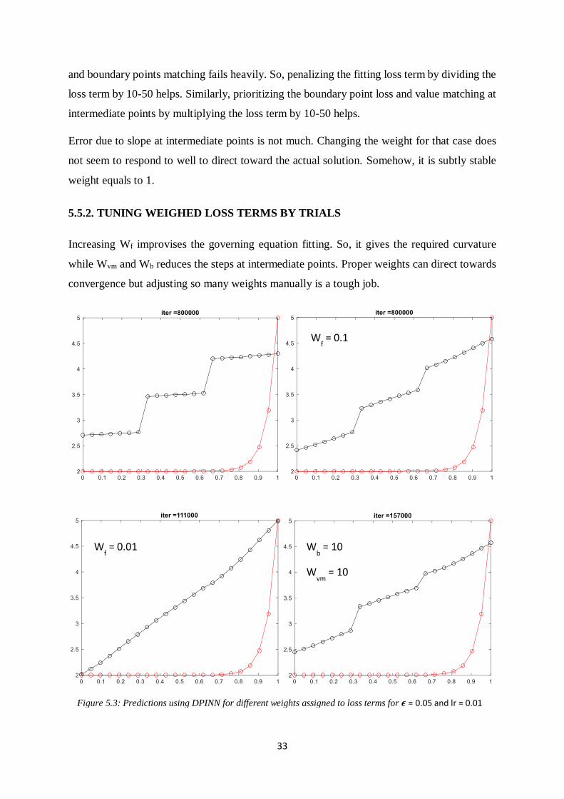
5.5.2. TUNING WEIGHED LOSS TERMS BY TRIALS

Increasing Wf improvises the governing equation fitting. So, it gives the required curvature

while Wvm and Wb reduces the steps at intermediate points. Proper weights can direct towards

convergence but adjusting so many weights manually is a tough job.

Wf = 0.1

Wf = 0.01 W

b = 10

Wvm

= 10

Figure 5.3: Predictions using DPINN for different weights assigned to loss terms for 𝝐 = 0.05 and lr = 0.01

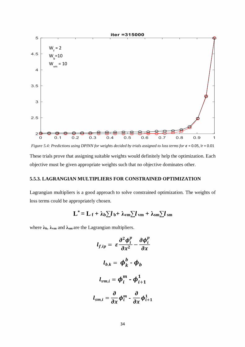
34

These trials prove that assigning suitable weights would definitely help the optimization. Each

objective must be given appropriate weights such that no objective dominates other.

5.5.3. LAGRANGIAN MULTIPLIERS FOR CONSTRAINED OPTIMIZATION

Lagrangian multipliers is a good approach to solve constrained optimization. The weights of

loss terms could be appropriately chosen.

L* = L f + λb∑l b+ λvm∑l vm + λsm∑l sm

where λb, λvm and λsm are the Lagrangian multipliers.

𝒍𝒇,𝒊𝒑 = 𝜺𝝏𝟐𝝓𝒊

𝒑

𝝏𝒙𝟐−

𝝏𝝓𝒊𝒑

𝝏𝒙

𝒍𝒃,𝒌 = 𝝓𝒌𝒃 - 𝝓𝒃

𝒍𝒗𝒎,𝒊 = 𝝓𝒊𝒎

- 𝝓𝒊+𝟏𝟏

𝒍𝒔𝒎,𝒊 =𝝏

𝝏𝒙𝝓𝒊

𝒎 - 𝝏

𝝏𝒙𝝓𝒊+𝟏

𝟏

Wf = 2

Wb=10

Wvm

= 10

Figure 5.4: Predictions using DPINN for weights decided by trials assigned to loss terms for 𝝐 = 0.05, lr = 0.01

35

Normal equations: 𝜵𝑳∗ = 𝟎

[ 𝜕∑𝑙𝑏

𝜕𝜔𝑖𝑗

𝜕∑𝑙𝑣𝑚

𝜕𝜔𝑖𝑗

𝜕∑𝑙𝑠𝑚

𝜕𝜔𝑖𝑗 ] [λ𝑏 λ𝑣𝑚 λ𝑠𝑚]𝑻 = [−∑𝑙𝑓

𝜕𝑙𝑓

𝜕𝜔𝑖𝑗]

𝝀 = (𝑨𝑻𝑨 )−𝟏𝑨𝑻𝑩

The Lagrange’s method cannot be exactly imposed in this problem. The result deteriorates in

this scheme.

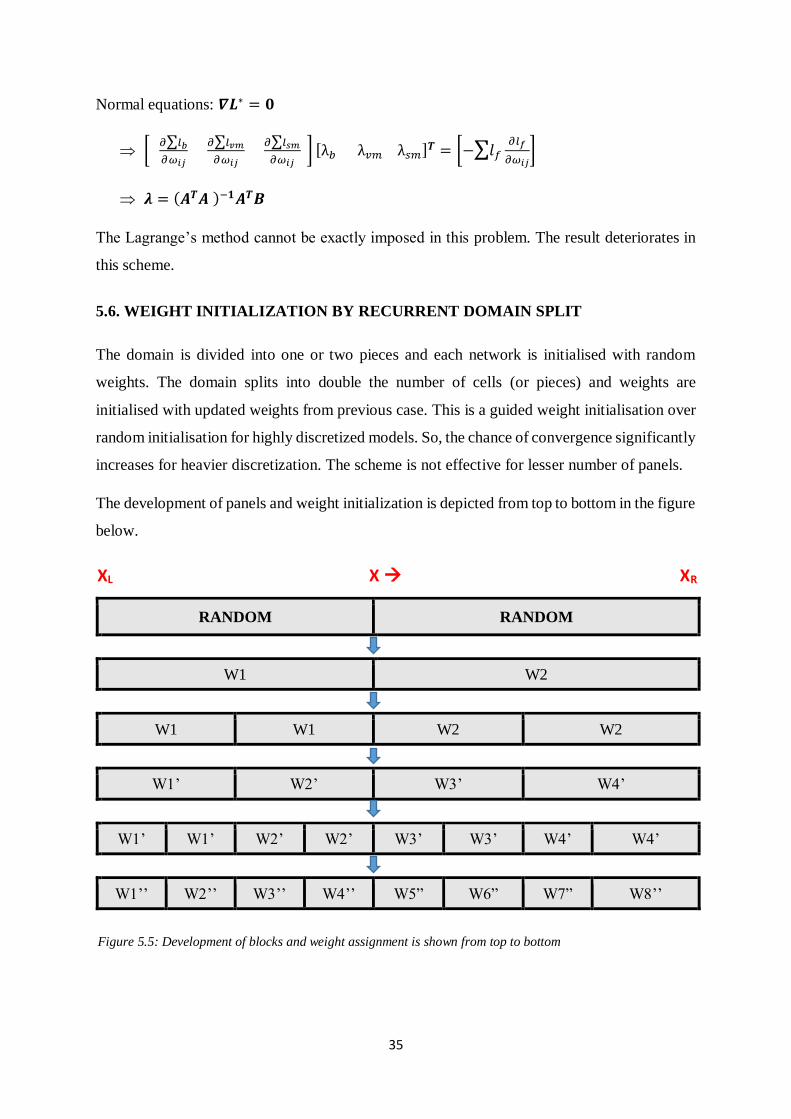
5.6. WEIGHT INITIALIZATION BY RECURRENT DOMAIN SPLIT

The domain is divided into one or two pieces and each network is initialised with random

weights. The domain splits into double the number of cells (or pieces) and weights are

initialised with updated weights from previous case. This is a guided weight initialisation over

random initialisation for highly discretized models. So, the chance of convergence significantly

increases for heavier discretization. The scheme is not effective for lesser number of panels.

The development of panels and weight initialization is depicted from top to bottom in the figure

below.

RANDOM RANDOM

W1 W2

W1 W1 W2 W2

W1’ W2’ W3’ W4’

W1’ W1’ W2’ W2’ W3’ W3’ W4’ W4’

W1’’ W2’’ W3’’ W4’’ W5” W6” W7” W8’’

XL X → XR

Figure 5.5: Development of blocks and weight assignment is shown from top to bottom

36

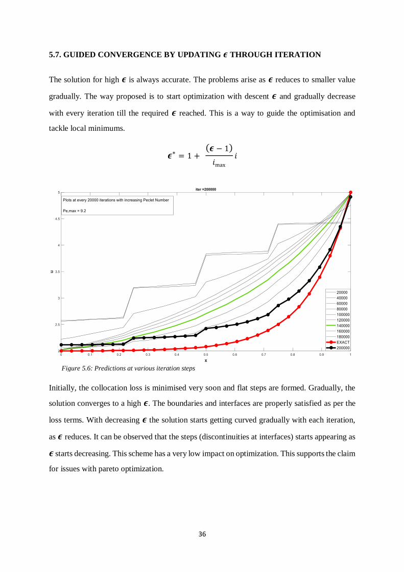
5.7. GUIDED CONVERGENCE BY UPDATING 𝝐 THROUGH ITERATION

The solution for high 𝝐 is always accurate. The problems arise as 𝝐 reduces to smaller value

gradually. The way proposed is to start optimization with descent 𝝐 and gradually decrease

with every iteration till the required 𝝐 reached. This is a way to guide the optimisation and

tackle local minimums.

𝝐∗ = 1 + (𝝐 − 1)

𝑖max

𝑖

Initially, the collocation loss is minimised very soon and flat steps are formed. Gradually, the

solution converges to a high 𝝐. The boundaries and interfaces are properly satisfied as per the

loss terms. With decreasing 𝝐 the solution starts getting curved gradually with each iteration,

as 𝝐 reduces. It can be observed that the steps (discontinuities at interfaces) starts appearing as

𝝐 starts decreasing. This scheme has a very low impact on optimization. This supports the claim

for issues with pareto optimization.

Figure 5.6: Predictions at various iteration steps

37

5.8.1. MODIFIED TRIAL FUNCTIONS WITH EXTRA LINEAR COMPONENT

Let the trial function have a linear component in the form:

𝝓(𝒙,𝝎, 𝒃) = 𝑨𝒙 + 𝑵𝑵(𝒙,𝒘, 𝒃)

Where,

𝝓 : new trial function

NN: old neural network

A: additional weight

The idea behind this approach is to guide the weights update to fit a straight line before the

network function starts capturing the trend. Addition of a new term ‘Ax’ helps the convergence

by guiding the weights towards linear fitting at early stage of learning. Can be tried with

dominatingly large value of A during weight initialization to increase the impact. Somehow,

this approach does not seem to be that effective during optimization

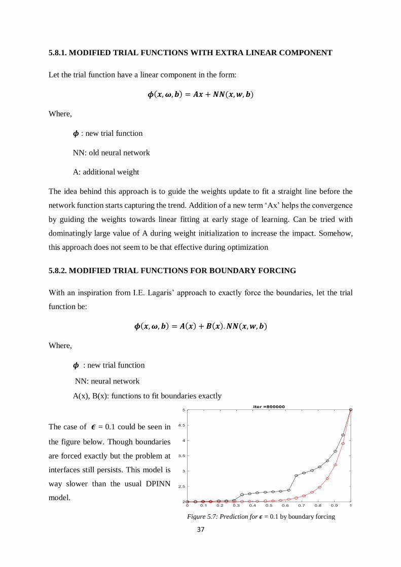
5.8.2. MODIFIED TRIAL FUNCTIONS FOR BOUNDARY FORCING

With an inspiration from I.E. Lagaris’ approach to exactly force the boundaries, let the trial

function be:

𝝓(𝒙,𝝎, 𝒃) = 𝑨(𝒙) + 𝑩(𝒙).𝑵𝑵(𝒙,𝒘, 𝒃)

Where,

𝝓 : new trial function

NN: neural network

A(x), B(x): functions to fit boundaries exactly

The case of 𝝐 = 0.1 could be seen in

the figure below. Though boundaries

are forced exactly but the problem at

interfaces still persists. This model is

way slower than the usual DPINN

model.

Figure 5.7: Prediction for 𝝐 = 0.1 by boundary forcing

38

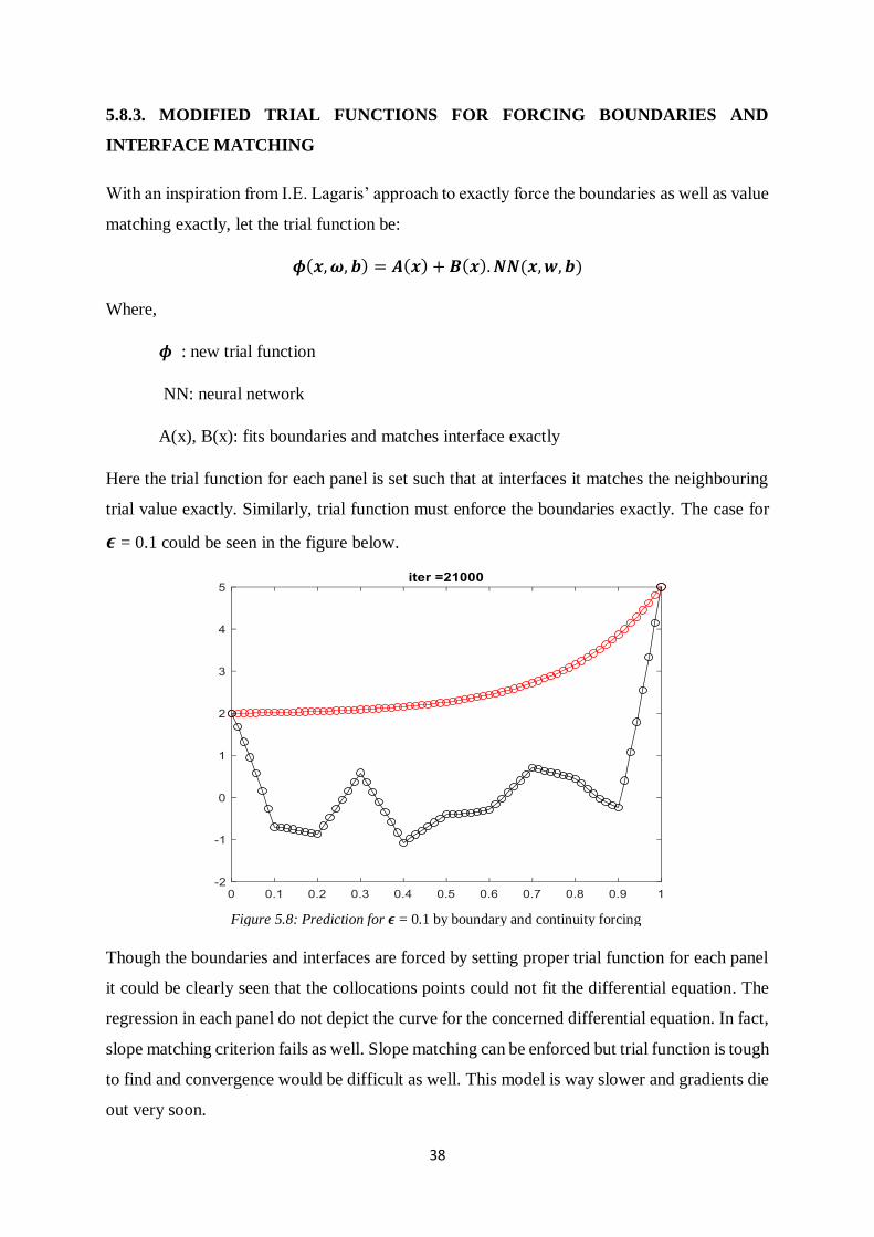
5.8.3. MODIFIED TRIAL FUNCTIONS FOR FORCING BOUNDARIES AND

INTERFACE MATCHING

With an inspiration from I.E. Lagaris’ approach to exactly force the boundaries as well as value

matching exactly, let the trial function be:

𝝓(𝒙,𝝎, 𝒃) = 𝑨(𝒙) + 𝑩(𝒙).𝑵𝑵(𝒙,𝒘, 𝒃)

Where,

𝝓 : new trial function

NN: neural network

A(x), B(x): fits boundaries and matches interface exactly

Here the trial function for each panel is set such that at interfaces it matches the neighbouring

trial value exactly. Similarly, trial function must enforce the boundaries exactly. The case for

𝝐 = 0.1 could be seen in the figure below.

Though the boundaries and interfaces are forced by setting proper trial function for each panel

it could be clearly seen that the collocations points could not fit the differential equation. The

regression in each panel do not depict the curve for the concerned differential equation. In fact,

slope matching criterion fails as well. Slope matching can be enforced but trial function is tough

to find and convergence would be difficult as well. This model is way slower and gradients die

out very soon.

Figure 5.8: Prediction for 𝝐 = 0.1 by boundary and continuity forcing

39

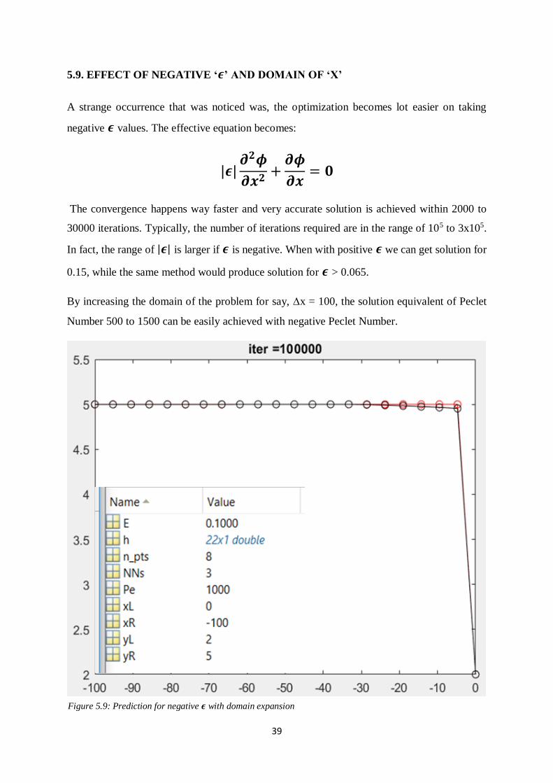
5.9. EFFECT OF NEGATIVE ‘𝝐’ AND DOMAIN OF ‘X’

A strange occurrence that was noticed was, the optimization becomes lot easier on taking

negative 𝝐 values. The effective equation becomes:

|𝝐|𝝏𝟐𝝓

𝝏𝒙𝟐+

𝝏𝝓

𝝏𝒙= 𝟎

The convergence happens way faster and very accurate solution is achieved within 2000 to

30000 iterations. Typically, the number of iterations required are in the range of 105 to 3x105.

In fact, the range of |𝝐| is larger if 𝝐 is negative. When with positive 𝝐 we can get solution for

0.15, while the same method would produce solution for 𝝐 > 0.065.

By increasing the domain of the problem for say, x = 100, the solution equivalent of Peclet

Number 500 to 1500 can be easily achieved with negative Peclet Number.

Figure 5.9: Prediction for negative 𝝐 with domain expansion

40

5.10. USING THE FLUX TERM FOR FORCING AT COLLOCATION POINTS

Flux = [𝜺𝝏𝝓𝒊

𝒎

𝝏𝒙 − 𝝓𝒊

𝒎]

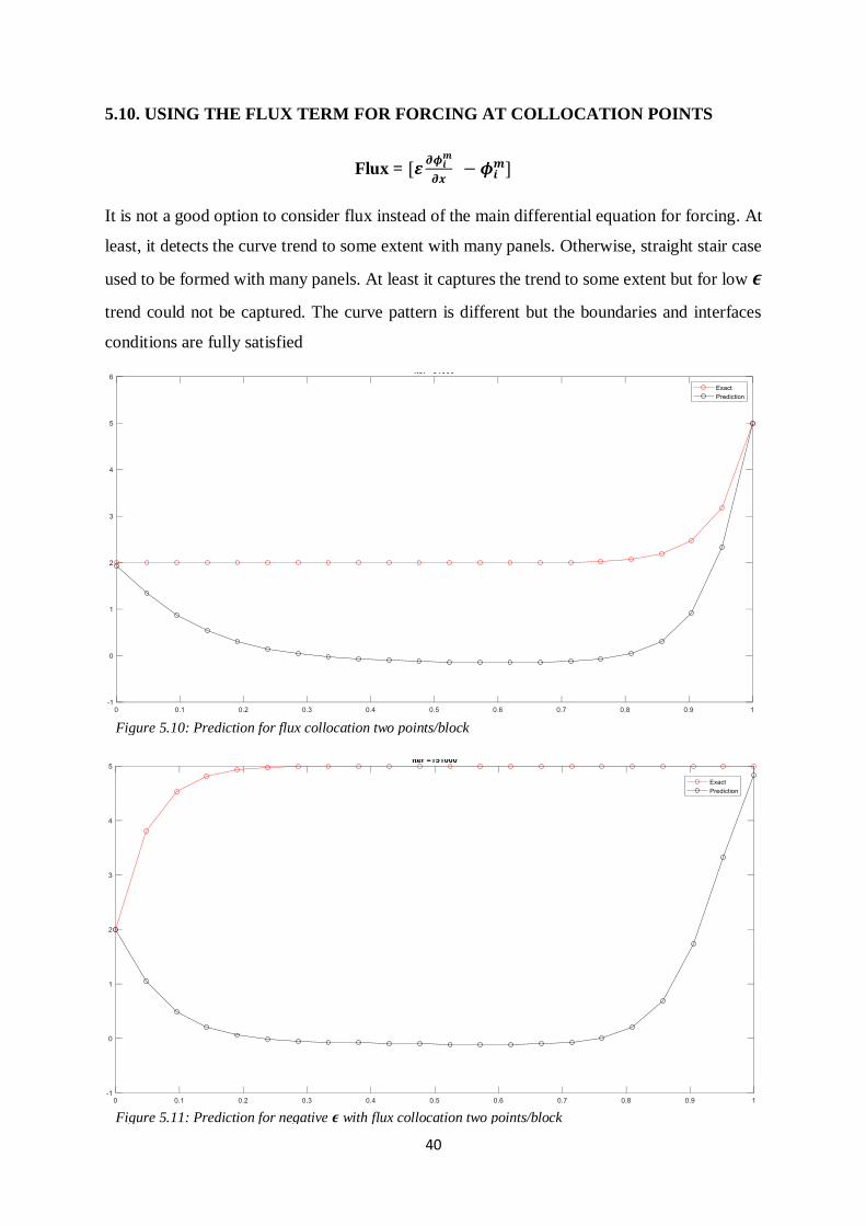
It is not a good option to consider flux instead of the main differential equation for forcing. At

least, it detects the curve trend to some extent with many panels. Otherwise, straight stair case

used to be formed with many panels. At least it captures the trend to some extent but for low 𝝐

trend could not be captured. The curve pattern is different but the boundaries and interfaces

conditions are fully satisfied

Figure 5.10: Prediction for flux collocation two points/block

Figure 5.11: Prediction for negative 𝝐 with flux collocation two points/block

41

5.11. LOSS TERM TREND WITH ITERATION

I. ROUGHLY APPROXIMATING CASE

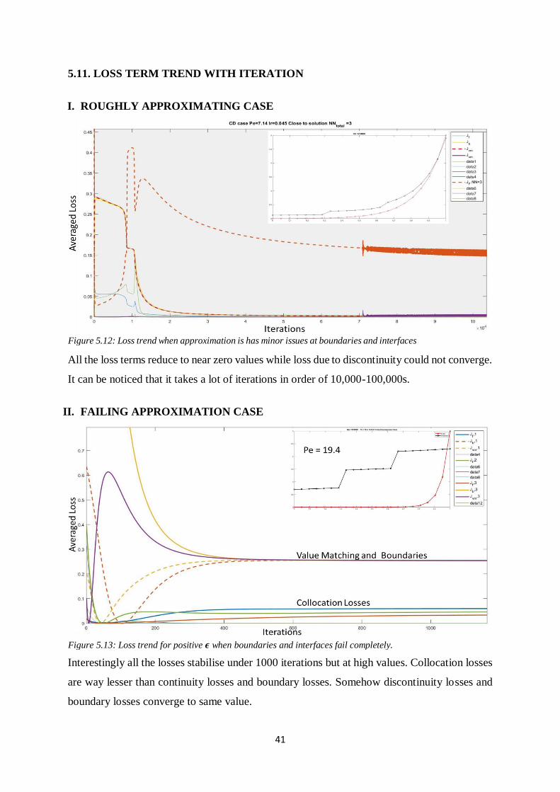
All the loss terms reduce to near zero values while loss due to discontinuity could not converge.

It can be noticed that it takes a lot of iterations in order of 10,000-100,000s.

II. FAILING APPROXIMATION CASE

Interestingly all the losses stabilise under 1000 iterations but at high values. Collocation losses

are way lesser than continuity losses and boundary losses. Somehow discontinuity losses and

boundary losses converge to same value.

Figure 5.12: Loss trend when approximation is has minor issues at boundaries and interfaces

Figure 5.13: Loss trend for positive 𝝐 when boundaries and interfaces fail completely.

42

III. NEGATIVE 𝝐 CONVERGING CASE

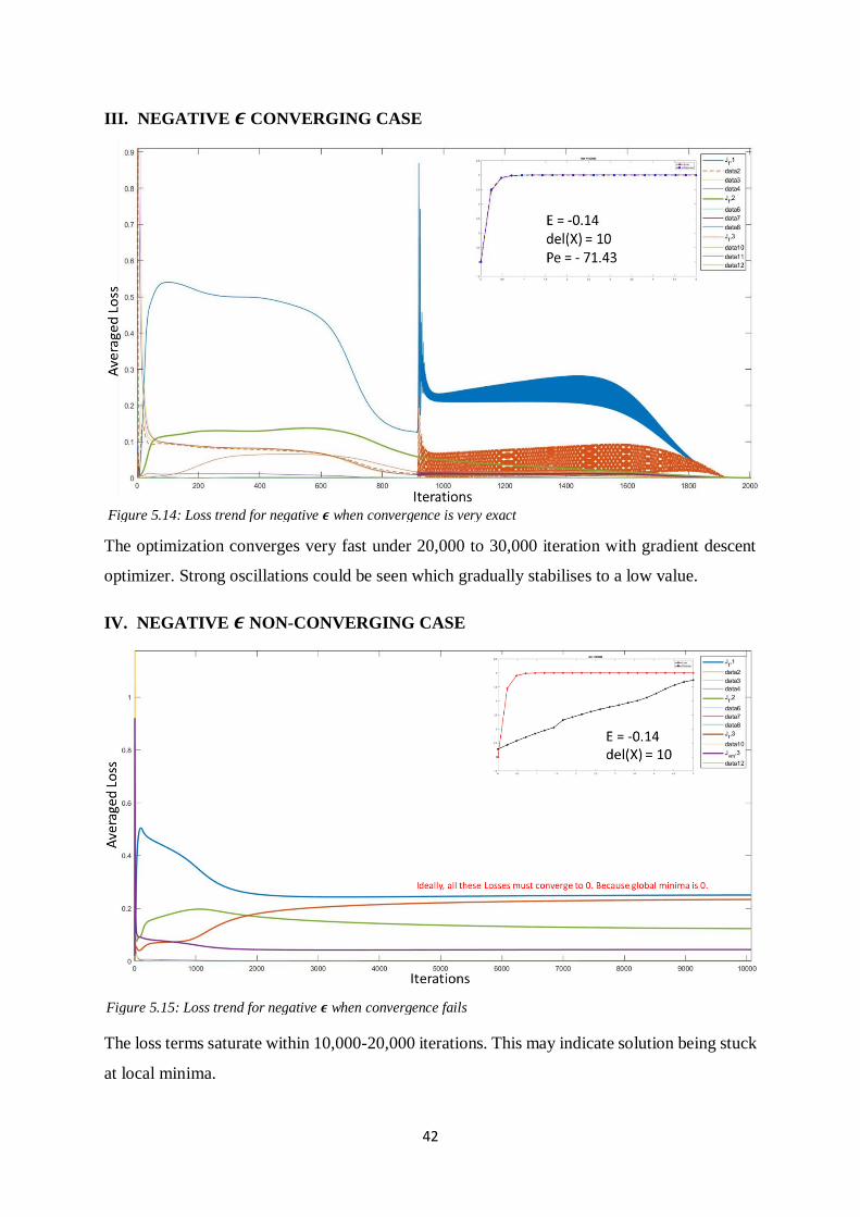
The optimization converges very fast under 20,000 to 30,000 iteration with gradient descent

optimizer. Strong oscillations could be seen which gradually stabilises to a low value.

IV. NEGATIVE 𝝐 NON-CONVERGING CASE

The loss terms saturate within 10,000-20,000 iterations. This may indicate solution being stuck

at local minima.

Figure 5.14: Loss trend for negative 𝝐 when convergence is very exact

Figure 5.15: Loss trend for negative 𝝐 when convergence fails

43

5.12. LOSS GRADIENT TREND WITH ITERATION

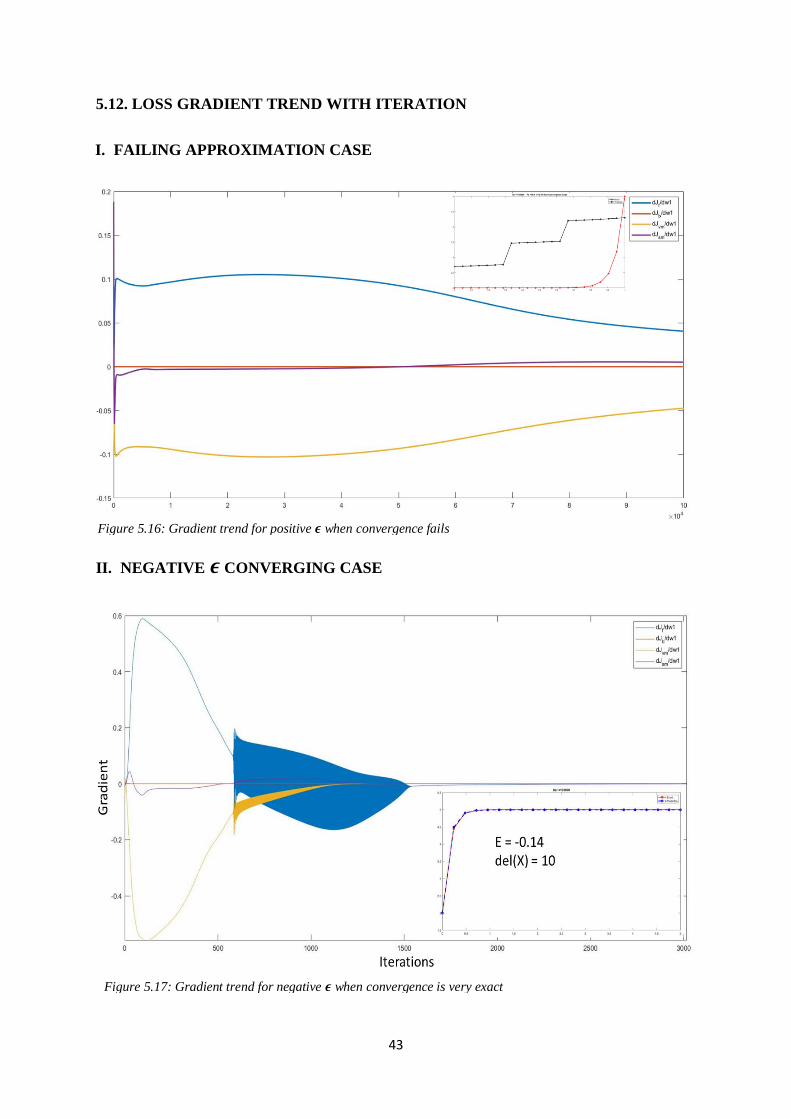
I. FAILING APPROXIMATION CASE

II. NEGATIVE 𝝐 CONVERGING CASE

Figure 5.17: Gradient trend for negative 𝝐 when convergence is very exact

Figure 5.16: Gradient trend for positive 𝝐 when convergence fails

44

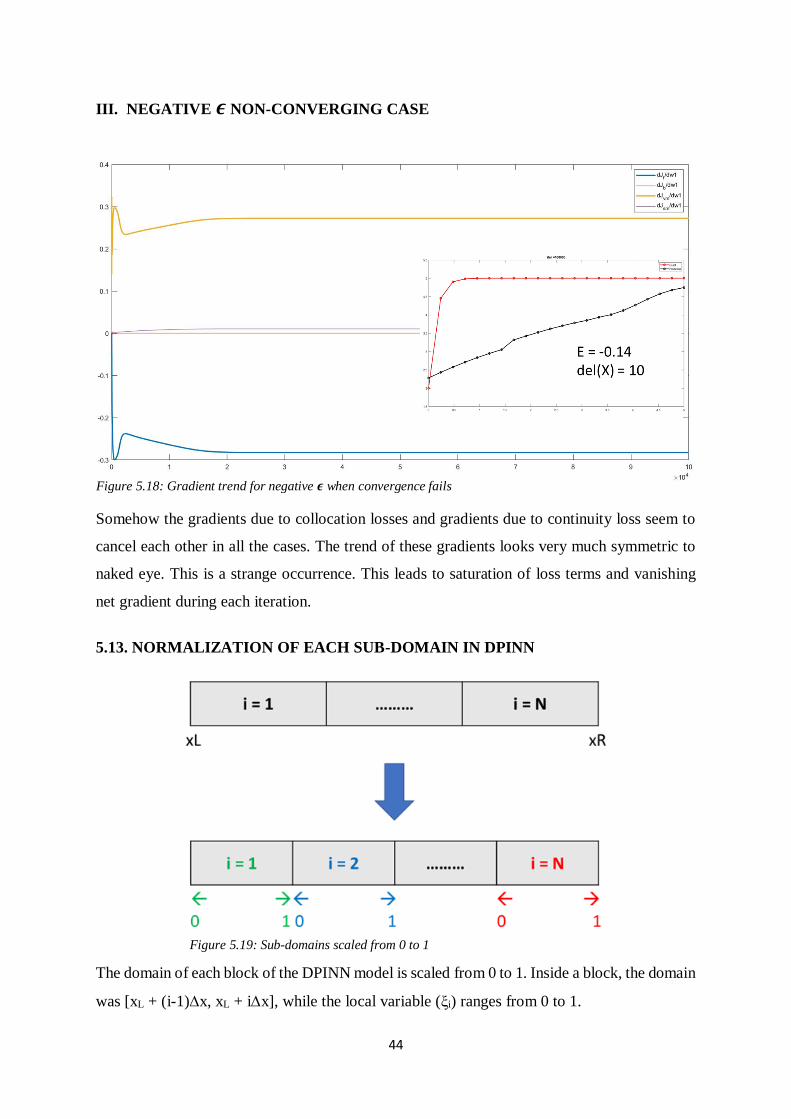
III. NEGATIVE 𝝐 NON-CONVERGING CASE

Somehow the gradients due to collocation losses and gradients due to continuity loss seem to

cancel each other in all the cases. The trend of these gradients looks very much symmetric to

naked eye. This is a strange occurrence. This leads to saturation of loss terms and vanishing

net gradient during each iteration.

5.13. NORMALIZATION OF EACH SUB-DOMAIN IN DPINN

The domain of each block of the DPINN model is scaled from 0 to 1. Inside a block, the domain

was [xL + (i-1)x, xL + ix], while the local variable (ξi) ranges from 0 to 1.

Figure 5.18: Gradient trend for negative 𝝐 when convergence fails

Figure 5.19: Sub-domains scaled from 0 to 1

45

Within the sub-domain:

x = xL + (i-1 + ξ i)x

=> dx = x.dξ i & (dx)2 = (x) 2.(d ξ i) 2

So, the differential equation becomes:

𝛆𝛛𝟐𝛟

𝛛𝐱𝟐−

𝛛𝛟

𝛛𝐱= 𝟎

=> 𝛆𝛛𝟐𝛟

(x) 2𝛛ξ i𝟐 −

𝛛𝛟

(x) 𝛛ξ i

= 𝟎

=> 𝛆𝛛𝟐𝛟

(x)𝛛ξ i𝟐 −

𝛛𝛟

𝛛ξ i

= 𝟎

=> (𝐍𝐁.𝛆

𝐱𝐑−𝐱𝐋)

𝛛𝟐𝛟

𝛛ξ i𝟐 −

𝛛𝛟

𝛛ξ i

= 𝟎

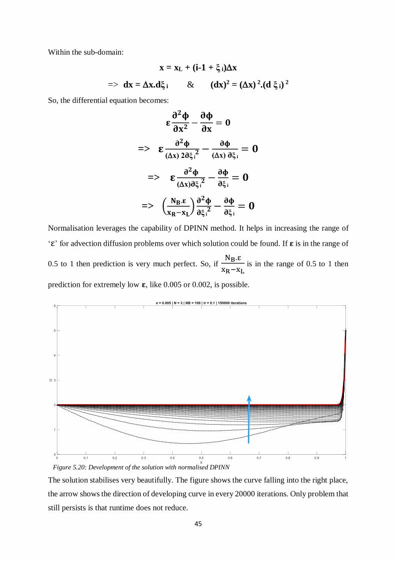
Normalisation leverages the capability of DPINN method. It helps in increasing the range of

‘ε’ for advection diffusion problems over which solution could be found. If 𝛆 is in the range of

0.5 to 1 then prediction is very much perfect. So, if NB.ε

xR−xL is in the range of 0.5 to 1 then

prediction for extremely low 𝛆, like 0.005 or 0.002, is possible.

The solution stabilises very beautifully. The figure shows the curve falling into the right place,

the arrow shows the direction of developing curve in every 20000 iterations. Only problem that

still persists is that runtime does not reduce.

Figure 5.20: Development of the solution with normalised DPINN

46

5.14. TESTS FOR FINDING ISSUES

Issues may have rose due to many problems but most probably due to either poor optimisation

or ill-posed algorithm for physics information (training). Various tests were conducted to figure

out if there is any error due to training.

• Linear Approximation by Solving Exactly Required Consistent Discrete Equations

• Linear Approximation by Norm Minimisation of Discrete Equations

• Quadratic Approximation by Norm Minimisation of Discrete Equations

• Optimization of Neural Network using Levenberg-Marquardt Algorithm

5.14.1. PIECEWISE LINEAR APPROXIMATION

Let us have N panels and approximating function in each panel be Y = Aix + Bi, where Ai and

Bi are to be determined to find the fit, where i = panel number.

Governing equations: ∈𝝏𝟐𝒀

𝝏𝒙𝟐 −

𝝏𝒀

𝝏𝒙 = 0 => 0 – Ai = 0 ( invalid )

So, Flux equation is used as governing equation: ∈𝝏𝒀

𝝏𝒙 − 𝒀= 0

=> ∈Ai – Aix – Bi = 0

Interface continuity equation,

Y(x=xi,R) = Y(x=xi+1,L)

=> Ai.xi,R + Bi = Ai+1.xi+1,L + Bi+1

Boundary equation,

Y(x=xL) = YL & Y(x=xR) = YR

=> A1.xL + B1 = YL & AN.xR + BN = YR

The number of unknowns that needs to be determined is 2N. For exact solution, 2N equations

are required to be solved. There are two compulsory equations for boundary conditions, N-1

compulsory equations for value match at interfaces for continuity. N – 1 more equations are

required for exact solution. So, N-1 distinct collocation points are used over governing

differential equation but there are infinite points for collocation so, equations will be

inconsistent.

47

Writing the equations in Matrix form, MX = C where X = coefficient matrix,

X = M-1.C

In case of inconsistent equations, M is not invertible. So, pseudoinverse of M is taken instead.

Penrose-Moore pseudoinverse solution give the solution in least-norm sense.

X = pinv(M).C

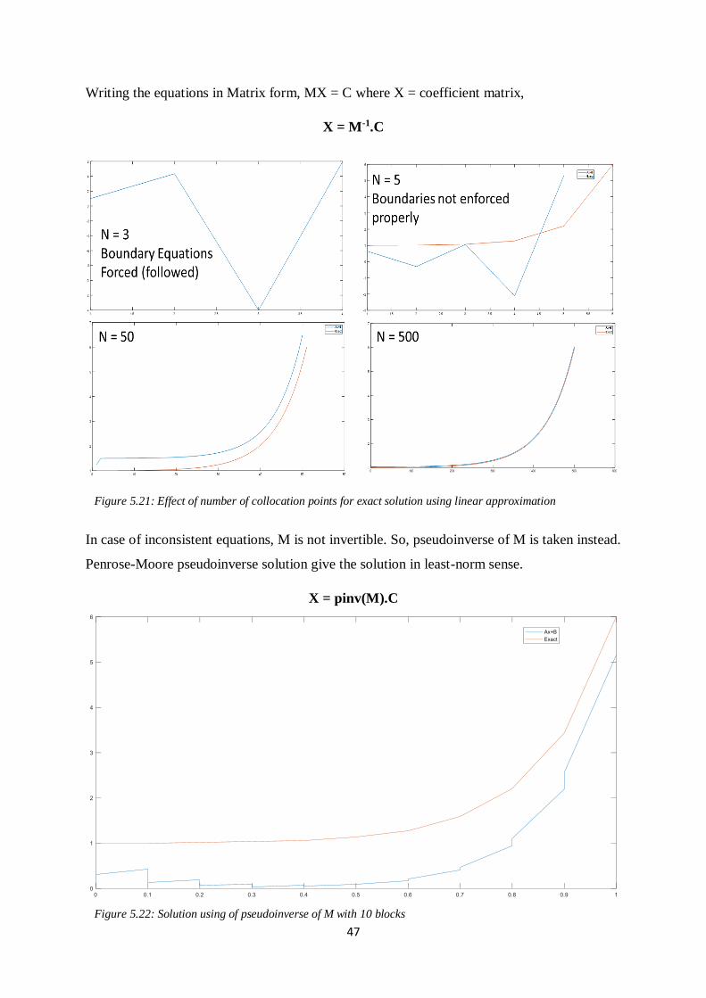
Figure 5.21: Effect of number of collocation points for exact solution using linear approximation

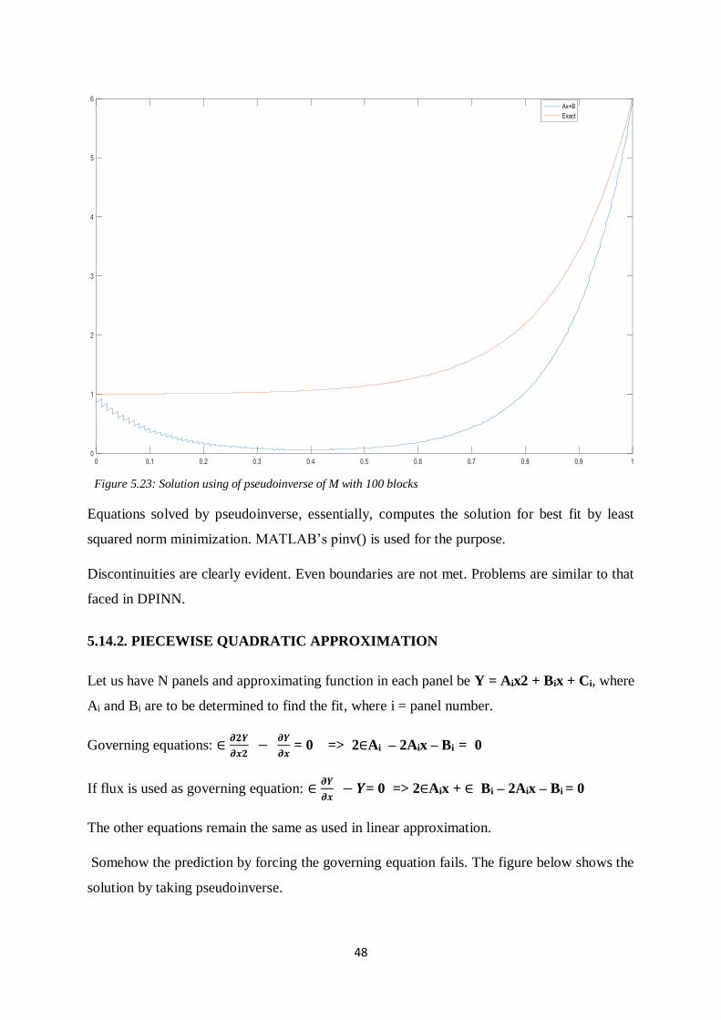
Figure 5.22: Solution using of pseudoinverse of M with 10 blocks

48

Equations solved by pseudoinverse, essentially, computes the solution for best fit by least

squared norm minimization. MATLAB’s pinv() is used for the purpose.

Discontinuities are clearly evident. Even boundaries are not met. Problems are similar to that

faced in DPINN.

5.14.2. PIECEWISE QUADRATIC APPROXIMATION

Let us have N panels and approximating function in each panel be Y = Aix2 + Bix + Ci, where

Ai and Bi are to be determined to find the fit, where i = panel number.

Governing equations: ∈𝝏𝟐𝒀

𝝏𝒙𝟐 −

𝝏𝒀

𝝏𝒙 = 0 => 2∈Ai – 2Aix – Bi = 0

If flux is used as governing equation: ∈𝝏𝒀

𝝏𝒙 − 𝒀= 0 => 2∈Aix + ∈ Bi – 2Aix – Bi = 0

The other equations remain the same as used in linear approximation.

Somehow the prediction by forcing the governing equation fails. The figure below shows the

solution by taking pseudoinverse.

Figure 5.23: Solution using of pseudoinverse of M with 100 blocks

49

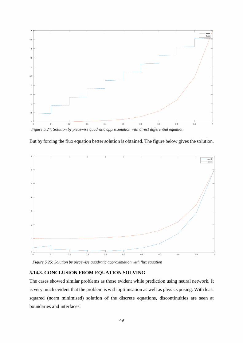
But by forcing the flux equation better solution is obtained. The figure below gives the solution.

5.14.3. CONCLUSION FROM EQUATION SOLVING

The cases showed similar problems as those evident while prediction using neural network. It

is very much evident that the problem is with optimisation as well as physics posing. With least

squared (norm minimised) solution of the discrete equations, discontinuities are seen at

boundaries and interfaces.

Figure 5.24: Solution by piecewise quadratic approximation with direct differential equation

Figure 5.25: Solution by piecewise quadratic approximation with flux equation

50

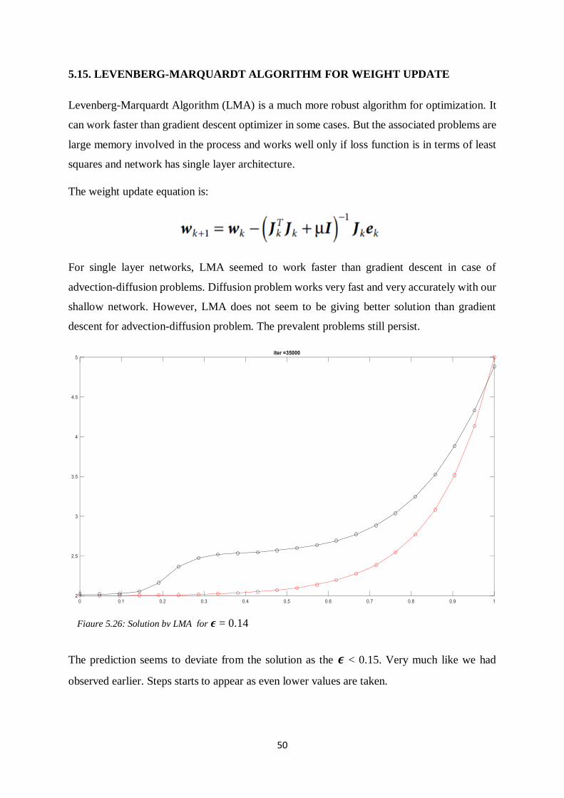
5.15. LEVENBERG-MARQUARDT ALGORITHM FOR WEIGHT UPDATE

Levenberg-Marquardt Algorithm (LMA) is a much more robust algorithm for optimization. It

can work faster than gradient descent optimizer in some cases. But the associated problems are

large memory involved in the process and works well only if loss function is in terms of least

squares and network has single layer architecture.

The weight update equation is:

For single layer networks, LMA seemed to work faster than gradient descent in case of

advection-diffusion problems. Diffusion problem works very fast and very accurately with our

shallow network. However, LMA does not seem to be giving better solution than gradient

descent for advection-diffusion problem. The prevalent problems still persist.

The prediction seems to deviate from the solution as the 𝝐 < 0.15. Very much like we had

observed earlier. Steps starts to appear as even lower values are taken.

Figure 5.26: Solution by LMA for 𝝐 = 0.14

51

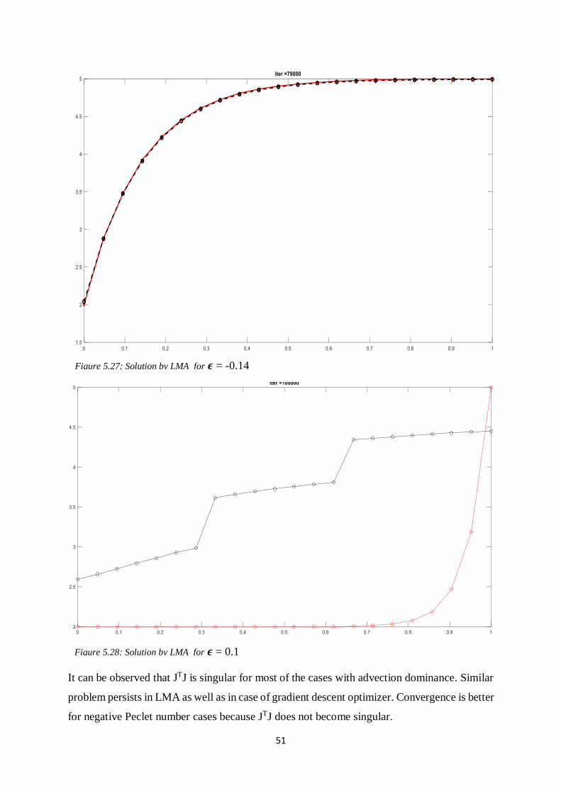
It can be observed that JTJ is singular for most of the cases with advection dominance. Similar

problem persists in LMA as well as in case of gradient descent optimizer. Convergence is better

for negative Peclet number cases because JTJ does not become singular.

Figure 5.27: Solution by LMA for 𝝐 = -0.14

Figure 5.28: Solution by LMA for 𝝐 = 0.1

52

CHAPTER 6

EXTREME LEARNING MACHINE BASED DPINN

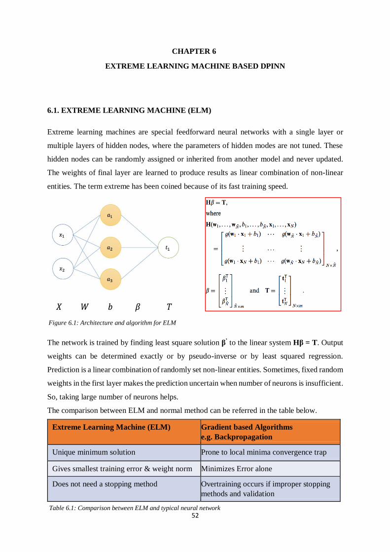
6.1. EXTREME LEARNING MACHINE (ELM)

Extreme learning machines are special feedforward neural networks with a single layer or

multiple layers of hidden nodes, where the parameters of hidden modes are not tuned. These

hidden nodes can be randomly assigned or inherited from another model and never updated.

The weights of final layer are learned to produce results as linear combination of non-linear

entities. The term extreme has been coined because of its fast training speed.

The network is trained by finding least square solution β’ to the linear system Hβ = T. Output

weights can be determined exactly or by pseudo-inverse or by least squared regression.

Prediction is a linear combination of randomly set non-linear entities. Sometimes, fixed random

weights in the first layer makes the prediction uncertain when number of neurons is insufficient.

So, taking large number of neurons helps.

The comparison between ELM and normal method can be referred in the table below.

Extreme Learning Machine (ELM) Gradient based Algorithms

e.g. Backpropagation

Unique minimum solution Prone to local minima convergence trap

Gives smallest training error & weight norm Minimizes Error alone

Does not need a stopping method Overtraining occurs if improper stopping

methods and validation

Figure 6.1: Architecture and algorithm for ELM

Table 6.1: Comparison between ELM and typical neural network

53

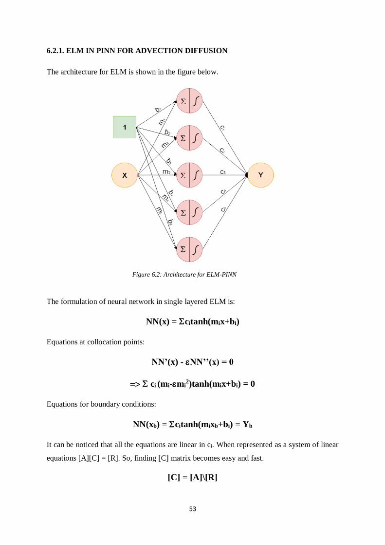
6.2.1. ELM IN PINN FOR ADVECTION DIFFUSION

The architecture for ELM is shown in the figure below.

The formulation of neural network in single layered ELM is:

NN(x) = citanh(mix+bi)

Equations at collocation points:

NN’(x) - NN’’(x) = 0

= ci (mi-mi2)tanh(mix+bi) = 0

Equations for boundary conditions:

NN(xb) = citanh(mixb+bi) = Yb

It can be noticed that all the equations are linear in ci. When represented as a system of linear

equations [A][C] = [R]. So, finding [C] matrix becomes easy and fast.

[C] = [A]\[R]

Figure 6.2: Architecture for ELM-PINN

54

If the number of collocation equations is N, and the number of boundary equations is 2 then

for exact solution, we need N+2 unknowns for exactness. So, N+2 neurons are taken in the

architecture.

ELM preserves the non-linearity but since only the second layer of weights are variable the

optimization objective becomes simpler. The set of equations are linear combinations of the

weights; hence the varying weights can be solved exactly if the number of neurons equals the

number of equations. There is no need for backpropagation. If a greater number of training

equations/points are taken than the number of neurons then least squared solution is a very

good approximate. This is the reason why this algorithm is way faster.

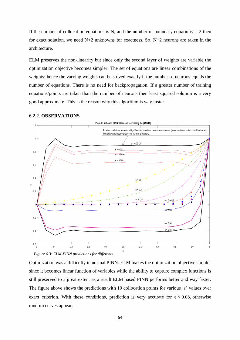
6.2.2. OBSERVATIONS

Optimization was a difficulty in normal PINN. ELM makes the optimization objective simpler

since it becomes linear function of variables while the ability to capture complex functions is

still preserved to a great extent as a result ELM based PINN performs better and way faster.

The figure above shows the predictions with 10 collocation points for various ‘’ values over

exact criterion. With these conditions, prediction is very accurate for otherwise

random curves appear.

Figure 6.3: ELM-PINN predictions for different

55

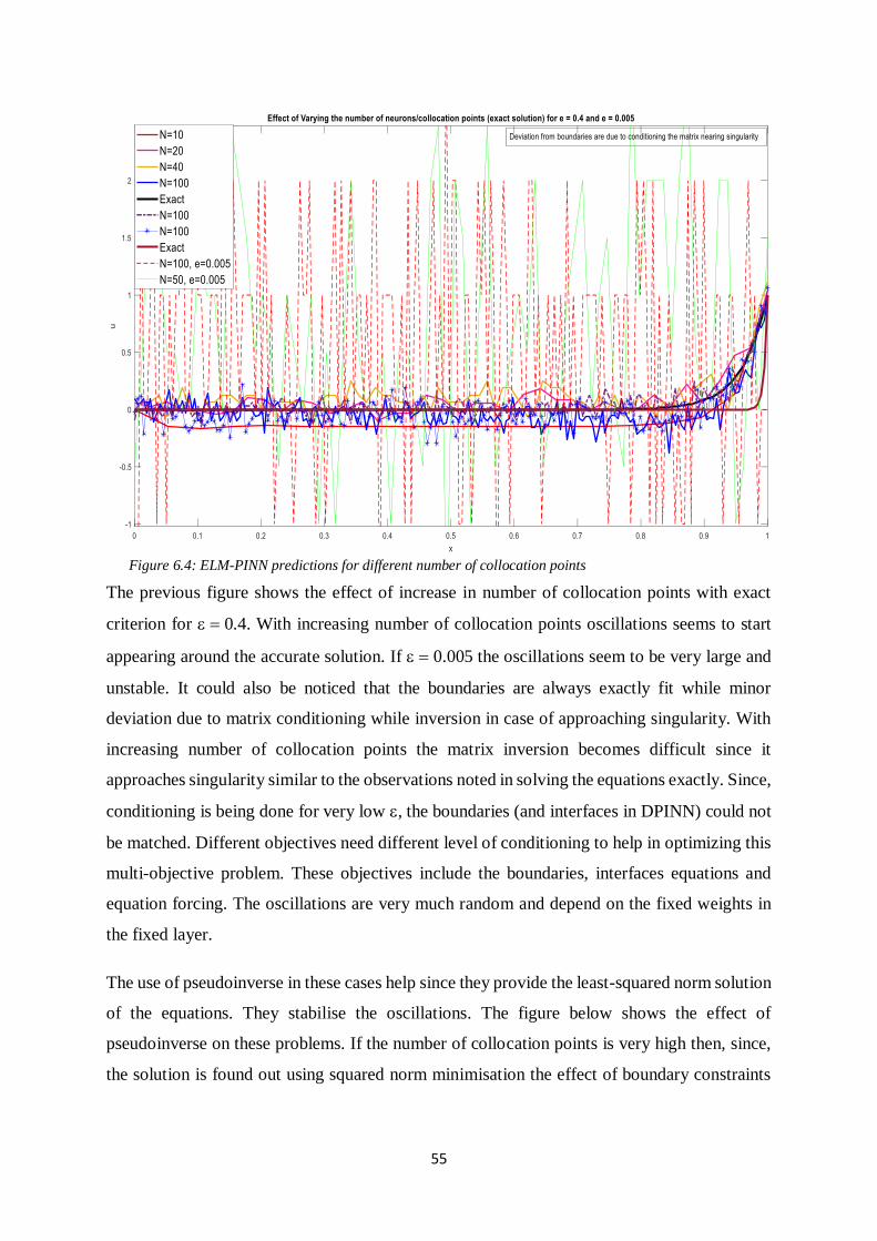
The previous figure shows the effect of increase in number of collocation points with exact

criterion for = 0.4. With increasing number of collocation points oscillations seems to start

appearing around the accurate solution. If = 0.005 the oscillations seem to be very large and

unstable. It could also be noticed that the boundaries are always exactly fit while minor

deviation due to matrix conditioning while inversion in case of approaching singularity. With

increasing number of collocation points the matrix inversion becomes difficult since it

approaches singularity similar to the observations noted in solving the equations exactly. Since,

conditioning is being done for very low , the boundaries (and interfaces in DPINN) could not

be matched. Different objectives need different level of conditioning to help in optimizing this

multi-objective problem. These objectives include the boundaries, interfaces equations and

equation forcing. The oscillations are very much random and depend on the fixed weights in

the fixed layer.

The use of pseudoinverse in these cases help since they provide the least-squared norm solution

of the equations. They stabilise the oscillations. The figure below shows the effect of

pseudoinverse on these problems. If the number of collocation points is very high then, since,

the solution is found out using squared norm minimisation the effect of boundary constraints

Figure 6.4: ELM-PINN predictions for different number of collocation points

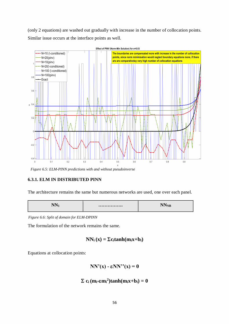
56

(only 2 equations) are washed out gradually with increase in the number of collocation points.

Similar issue occurs at the interface points as well.

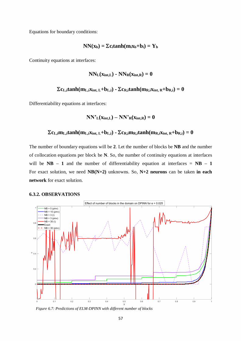
6.3.1. ELM IN DISTRIBUTED PINN

The architecture remains the same but numerous networks are used, one over each panel.

NN1 ……………. NNNB

The formulation of the network remains the same.

NNi (x) = citanh(mix+bi)

Equations at collocation points:

NN’(x) - NN’’(x) = 0

ci (mi-mi2)tanh(mix+bi) = 0

Figure 6.5: ELM-PINN predictions with and without pseudoinverse

Figure 6.6: Split of domain for ELM-DPINN

57

Equations for boundary conditions:

NN(xb) = citanh(mixb+bi) = Yb

Continuity equations at interfaces:

NNL(xint,L) - NNR(xint,R) = 0

cL,itanh(mL,ixint, L+bL,i) - cR,itanh(mR,ixint, R+bR,i) = 0

Differentiability equations at interfaces:

NN’L(xint,L) – NN’R(xint,R) = 0

cL,imL,itanh(mL,ixint, L+bL,i) - cR,imR,itanh(mR,ixint, R+bR,i) = 0

The number of boundary equations will be 2. Let the number of blocks be NB and the number

of collocation equations per block be N. So, the number of continuity equations at interfaces

will be NB – 1 and the number of differentiability equation at interfaces = NB – 1

For exact solution, we need NB(N+2) unknowns. So, N+2 neurons can be taken in each

network for exact solution.

6.3.2. OBSERVATIONS

Figure 6.7: Predictions of ELM-DPINN with different number of blocks

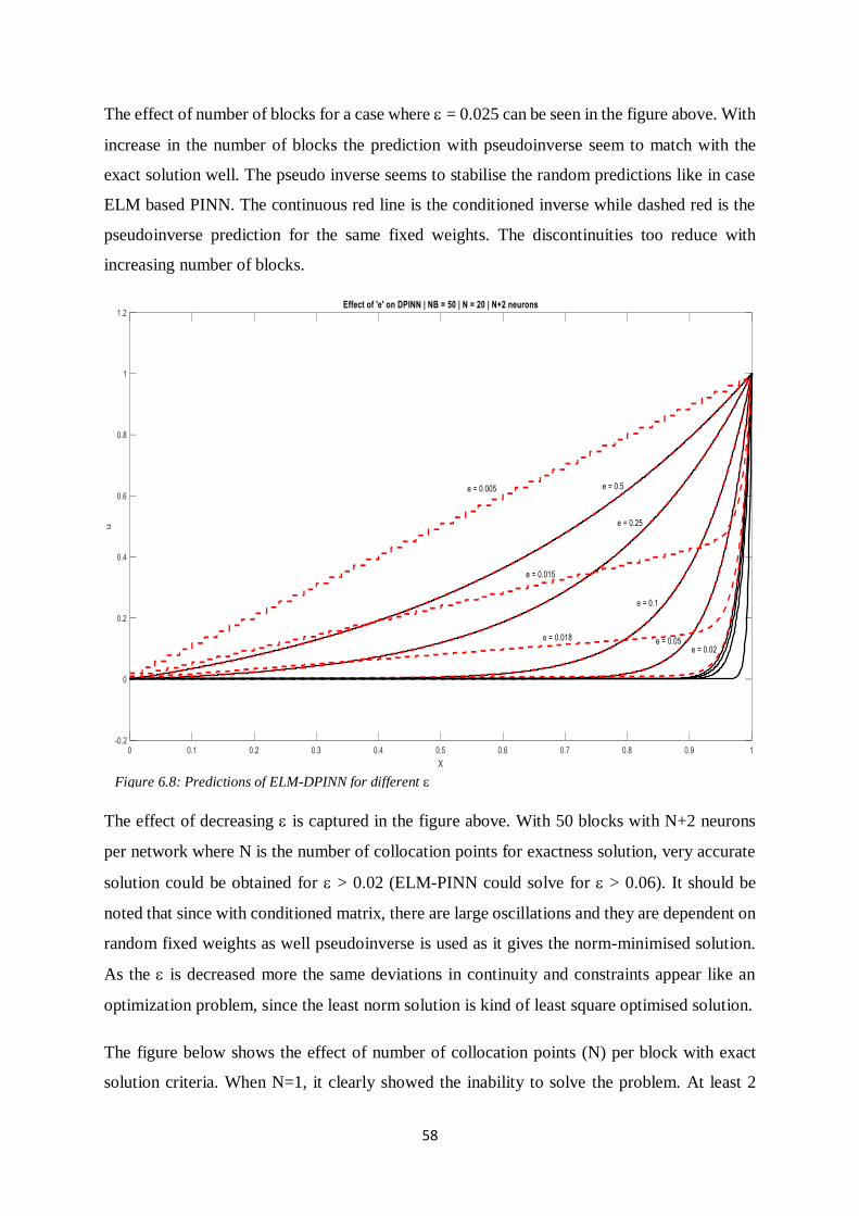
58

The effect of number of blocks for a case where = 0.025 can be seen in the figure above. With

increase in the number of blocks the prediction with pseudoinverse seem to match with the

exact solution well. The pseudo inverse seems to stabilise the random predictions like in case

ELM based PINN. The continuous red line is the conditioned inverse while dashed red is the

pseudoinverse prediction for the same fixed weights. The discontinuities too reduce with

increasing number of blocks.

The effect of decreasing is captured in the figure above. With 50 blocks with N+2 neurons

per network where N is the number of collocation points for exactness solution, very accurate

solution could be obtained for > 0.02 (ELM-PINN could solve for > 0.06). It should be

noted that since with conditioned matrix, there are large oscillations and they are dependent on

random fixed weights as well pseudoinverse is used as it gives the norm-minimised solution.

As the is decreased more the same deviations in continuity and constraints appear like an

optimization problem, since the least norm solution is kind of least square optimised solution.

The figure below shows the effect of number of collocation points (N) per block with exact

solution criteria. When N=1, it clearly showed the inability to solve the problem. At least 2

Figure 6.8: Predictions of ELM-DPINN for different

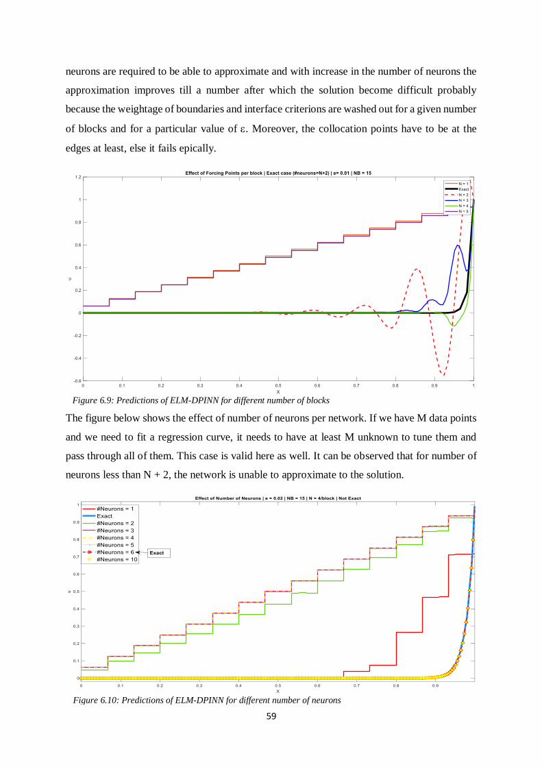
59

neurons are required to be able to approximate and with increase in the number of neurons the

approximation improves till a number after which the solution become difficult probably

because the weightage of boundaries and interface criterions are washed out for a given number

of blocks and for a particular value of . Moreover, the collocation points have to be at the

edges at least, else it fails epically.

The figure below shows the effect of number of neurons per network. If we have M data points

and we need to fit a regression curve, it needs to have at least M unknown to tune them and

pass through all of them. This case is valid here as well. It can be observed that for number of

neurons less than N + 2, the network is unable to approximate to the solution.

Figure 6.9: Predictions of ELM-DPINN for different number of blocks

Figure 6.10: Predictions of ELM-DPINN for different number of neurons

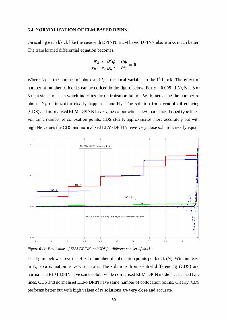
60

6.4. NORMALIZATION OF ELM BASED DPINN

On scaling each block like the case with DPINN, ELM based DPINN also works much better.

The transformed differential equation becomes,

𝑵𝑩. 𝜺

𝒙𝑹 − 𝒙𝑳

𝝏𝟐𝝓

𝝏ξ i𝟐 −

𝝏𝝓

𝝏ξ i

= 𝟎

Where NB is the number of block and ξi is the local variable in the ith block. The effect of

number of number of blocks can be noticed in the figure below. For 𝜺 = 0.005, if NB is is 3 or

5 then steps are seen which indicates the optimization failure. With increasing the number of

blocks NB optimization clearly happens smoothly. The solution from central differencing

(CDS) and normalised ELM-DPINN have same colour while CDS model has dashed type lines.

For same number of collocation points, CDS clearly approximates more accurately but with

high NB values the CDS and normalised ELM-DPINN have very close solution, nearly equal.

The figure below shows the effect of number of collocation points per block (N). With increase

in N, approximation is very accurate. The solutions from central differencing (CDS) and

normalised ELM-DPIN have same colour while normalised ELM-DPIN model has dashed type

lines. CDS and normalised ELM-DPIN have same number of collocation points. Clearly, CDS

performs better but with high values of N solutions are very close and accurate.

Figure 6.11: Predictions of ELM-DPINN and CDS for different number of blocks

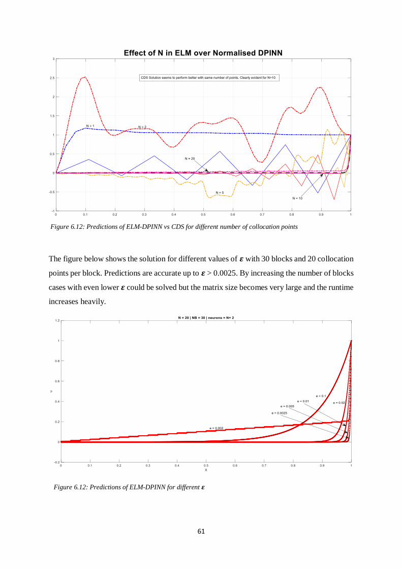
61

The figure below shows the solution for different values of 𝜺 with 30 blocks and 20 collocation

points per block. Predictions are accurate up to 𝜺 > 0.0025. By increasing the number of blocks

cases with even lower 𝜺 could be solved but the matrix size becomes very large and the runtime

increases heavily.

Figure 6.12: Predictions of ELM-DPINN vs CDS for different number of collocation points

Figure 6.12: Predictions of ELM-DPINN for different 𝜺

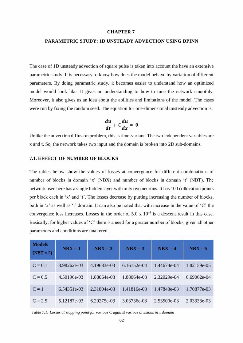
62

CHAPTER 7

PARAMETRIC STUDY: 1D UNSTEADY ADVECTION USING DPINN

The case of 1D unsteady advection of square pulse is taken into account the have an extensive

parametric study. It is necessary to know how does the model behave by variation of different

parameters. By doing parametric study, it becomes easier to understand how an optimized

model would look like. It gives an understanding to how to tune the network smoothly.

Moreover, it also gives us an idea about the abilities and limitations of the model. The cases

were run by fixing the random seed. The equation for one-dimensional unsteady advection is,

𝒅𝒖

𝒅𝒕+ ∁

𝒅𝒖

𝒅𝒙= 𝟎

Unlike the advection diffusion problem, this is time-variant. The two independent variables are

x and t. So, the network takes two input and the domain is broken into 2D sub-domains.

7.1. EFFECT OF NUMBER OF BLOCKS

The tables below show the values of losses at convergence for different combinations of

number of blocks in domain ‘x’ (NBX) and number of blocks in domain ‘t’ (NBT). The

network used here has a single hidden layer with only two neurons. It has 100 collocation points

per block each in ‘x’ and ‘t’. The losses decrease by putting increasing the number of blocks,

both in ‘x’ as well as ‘t’ domain. It can also be noted that with increase in the value of ‘C’ the

convergence loss increases. Losses in the order of 5.0 x 10-4 is a descent result in this case.

Basically, for higher values of ‘C’ there is a need for a greater number of blocks, given all other

parameters and conditions are unaltered.

Models

(NBT = 5) NBX = 1 NBX = 2 NBX = 3 NBX = 4 NBX = 5

C = 0.1 3.98262e-03 4.19683e-03 6.16152e-04 1.44674e-04 1.82159e-05

C = 0.5 4.50196e-03 1.88064e-03 1.88064e-03 2.32029e-04 6.69062e-04

C = 1 6.54351e-03 2.31804e-03 1.41816e-03 1.47843e-03 1.70877e-03

C = 2.5 5.12187e-03 6.20275e-03 3.03736e-03 2.53500e-03 2.03333e-03

Table 7.1: Losses at stopping point for various C against various divisions in x domain

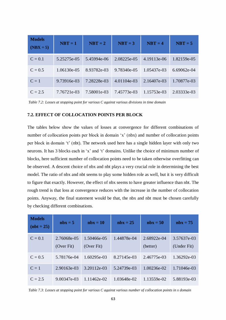
63

Models

(NBX = 5) NBT = 1 NBT = 2 NBT = 3 NBT = 4 NBT = 5

C = 0.1 5.25275e-05 5.45994e-06 2.08225e-05 4.19113e-06 1.82159e-05

C = 0.5 1.06130e-05 8.93782e-03 9.78340e-05 1.05437e-03 6.69062e-04

C = 1 9.73916e-03 7.28228e-03 4.01104e-03 2.16407e-03 1.70877e-03

C = 2.5 7.76721e-03 7.58001e-03 7.45773e-03 1.15753e-03 2.03333e-03

7.2. EFFECT OF COLLOCATION POINTS PER BLOCK

The tables below show the values of losses at convergence for different combinations of

number of collocation points per block in domain ‘x’ (nbx) and number of collocation points

per block in domain ‘t’ (nbt). The network used here has a single hidden layer with only two

neurons. It has 3 blocks each in ‘x’ and ‘t’ domains. Unlike the choice of minimum number of

blocks, here sufficient number of collocation points need to be taken otherwise overfitting can

be observed. A descent choice of nbx and nbt plays a very crucial role in determining the best

model. The ratio of nbx and nbt seems to play some hidden role as well, but it is very difficult

to figure that exactly. However, the effect of nbx seems to have greater influence than nbt. The

rough trend is that loss at convergence reduces with the increase in the number of collocation

points. Anyway, the final statement would be that, the nbx and nbt must be chosen carefully

by checking different combinations.

Models

(nbt = 25) nbx = 5 nbx = 10 nbx = 25 nbx = 50 nbx = 75

C = 0.1 2.76068e-05

(Over Fit)

1.50466e-05

(Over Fit)

1.44878e-04 2.68922e-04

(better)

3.57637e-03

(Under Fit)

C = 0.5 5.78176e-04 1.60295e-03 8.27145e-03 2.46775e-03 1.36292e-03

C = 1 2.90163e-03 3.20112e-03 5.24739e-03 1.00236e-02 1.71046e-03

C = 2.5 9.00347e-03 1.11462e-02 1.03648e-02 1.13559e-02 5.88193e-03

Table 7.2: Losses at stopping point for various C against various divisions in time domain

Table 7.3: Losses at stopping point for various C against various number of collocation points in x domain

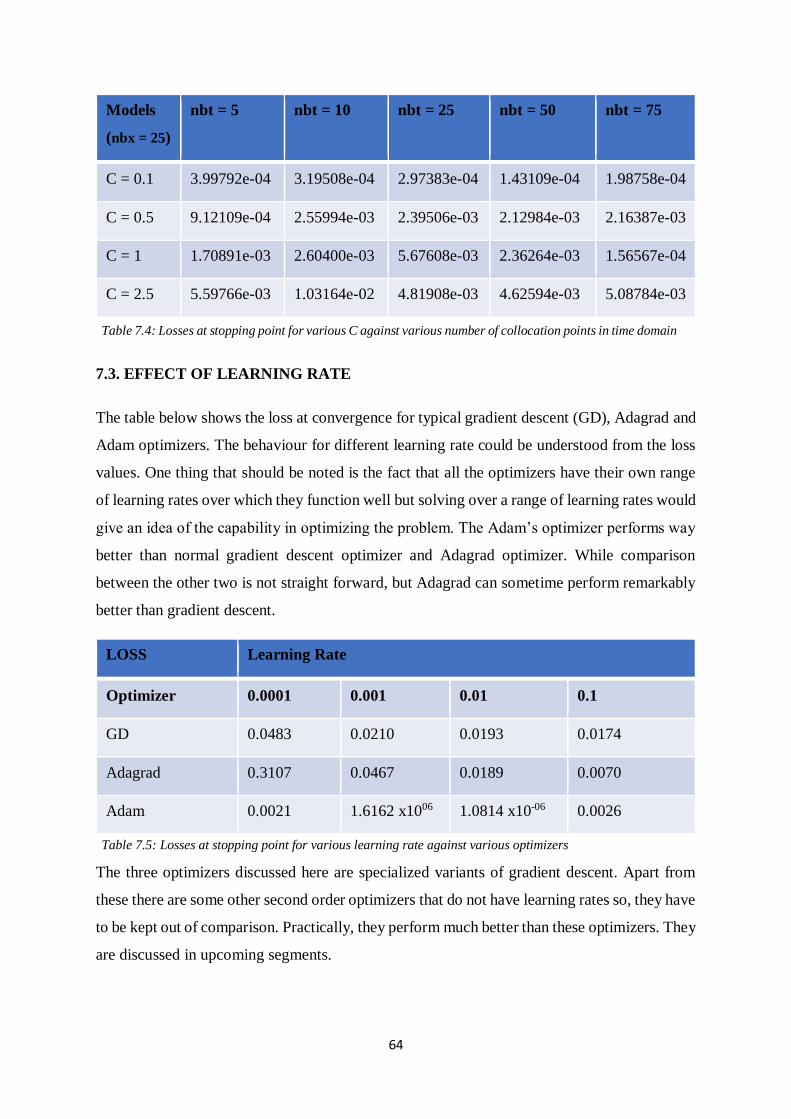
64

Models

(nbx = 25)

nbt = 5 nbt = 10 nbt = 25 nbt = 50 nbt = 75

C = 0.1 3.99792e-04 3.19508e-04 2.97383e-04 1.43109e-04 1.98758e-04

C = 0.5 9.12109e-04 2.55994e-03 2.39506e-03 2.12984e-03 2.16387e-03

C = 1 1.70891e-03 2.60400e-03 5.67608e-03 2.36264e-03 1.56567e-04

C = 2.5 5.59766e-03 1.03164e-02 4.81908e-03 4.62594e-03 5.08784e-03

7.3. EFFECT OF LEARNING RATE

The table below shows the loss at convergence for typical gradient descent (GD), Adagrad and

Adam optimizers. The behaviour for different learning rate could be understood from the loss

values. One thing that should be noted is the fact that all the optimizers have their own range

of learning rates over which they function well but solving over a range of learning rates would

give an idea of the capability in optimizing the problem. The Adam’s optimizer performs way

better than normal gradient descent optimizer and Adagrad optimizer. While comparison

between the other two is not straight forward, but Adagrad can sometime perform remarkably

better than gradient descent.

LOSS Learning Rate

Optimizer 0.0001 0.001 0.01 0.1

GD 0.0483 0.0210 0.0193 0.0174

Adagrad 0.3107 0.0467 0.0189 0.0070

Adam 0.0021 1.6162 x1006 1.0814 x10-06 0.0026

The three optimizers discussed here are specialized variants of gradient descent. Apart from

these there are some other second order optimizers that do not have learning rates so, they have

to be kept out of comparison. Practically, they perform much better than these optimizers. They

are discussed in upcoming segments.

Table 7.4: Losses at stopping point for various C against various number of collocation points in time domain

Table 7.5: Losses at stopping point for various learning rate against various optimizers

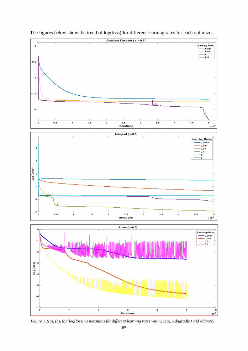
65

The figures below show the trend of log(loss) for different learning rates for each optimizer.

Figure 7.1(a), (b), (c): log(loss) vs iterations for different learning rates with GD(a), Adagrad(b) and Adam(c)

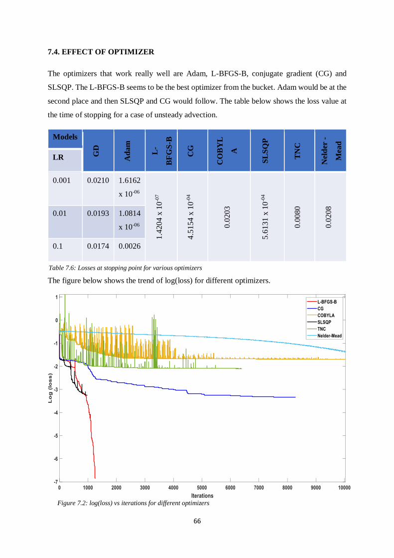
66

7.4. EFFECT OF OPTIMIZER

The optimizers that work really well are Adam, L-BFGS-B, conjugate gradient (CG) and

SLSQP. The L-BFGS-B seems to be the best optimizer from the bucket. Adam would be at the

second place and then SLSQP and CG would follow. The table below shows the loss value at

the time of stopping for a case of unsteady advection.

Models

GD

Ad

am

L-

BF

GS

-B

CG

CO

BY

L

A

SL

SQ

P

TN

C

Nel

der

-

Mea

d

LR

0.001 0.0210 1.6162

x 10-06

1.4

204 x

10

-07

4.5

154 x

10

-04

0.0

203

5.6

131 x

10

-04

0.0

080

0.0

208

0.01 0.0193 1.0814

x 10-06

0.1 0.0174 0.0026

The figure below shows the trend of log(loss) for different optimizers.

Figure 7.2: log(loss) vs iterations for different optimizers

Table 7.6: Losses at stopping point for various optimizers

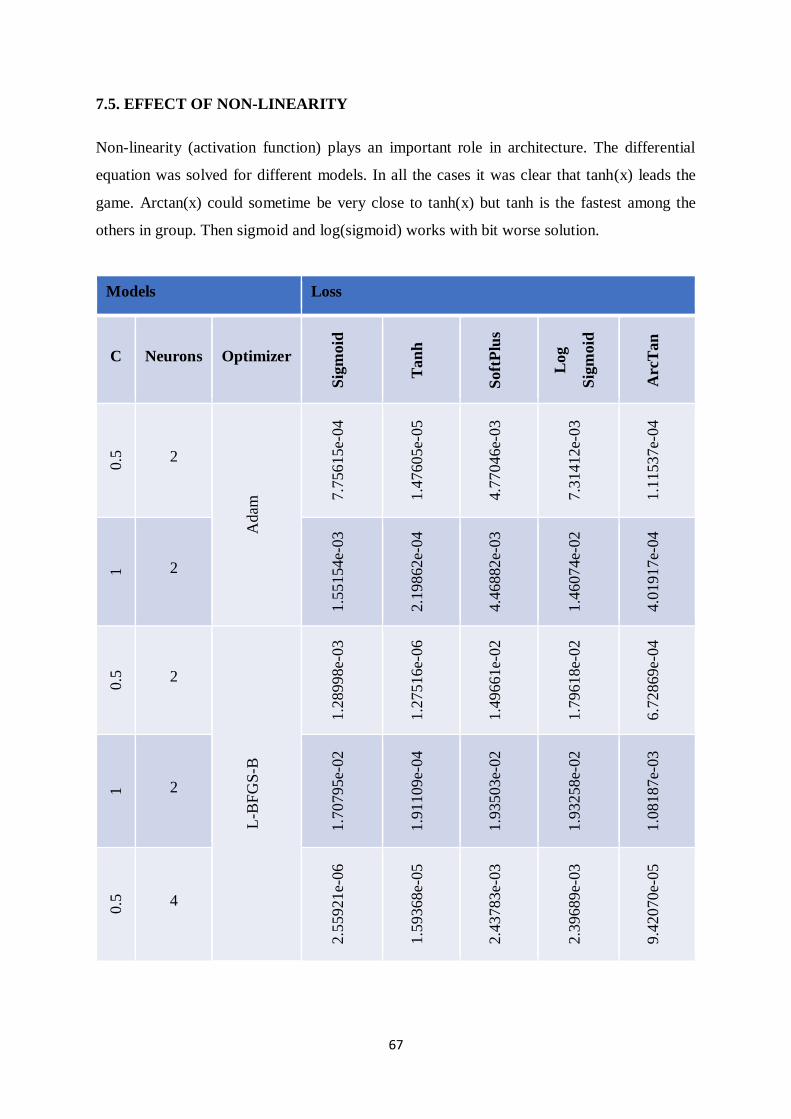
67

7.5. EFFECT OF NON-LINEARITY

Non-linearity (activation function) plays an important role in architecture. The differential

equation was solved for different models. In all the cases it was clear that tanh(x) leads the

game. Arctan(x) could sometime be very close to tanh(x) but tanh is the fastest among the

others in group. Then sigmoid and log(sigmoid) works with bit worse solution.

Models Loss

C Neurons Optimizer

Sig

moid

Tan

h

Soft

Plu

s

Log

Sig

moid

Arc

Tan

0.5

2

Adam

7.7

5615e-

04

1.4

7605e-

05

4.7

7046e-

03

7.3

1412e-

03

1.1

1537e-

04

1 2

1.5

5154e-

03

2.1

9862e-

04

4.4

6882e-

03

1.4

6074e-

02

4.0

1917e-

04

0.5

2

L-B

FG

S-B

1.2

8998e-

03

1.2

7516e-

06

1.4

9661e-

02

1.7

9618e-

02

6.7

2869e-

04

1 2

1.7

0795e-

02

1.9

1109e-

04

1.9

3503e-

02

1.9

3258e-

02

1.0

8187e-

03

0.5

4

2.5

5921e-

06

1.5

9368e-

05

2.4

3783e-

03

2.3

9689e-

03

9.4

2070e-

05

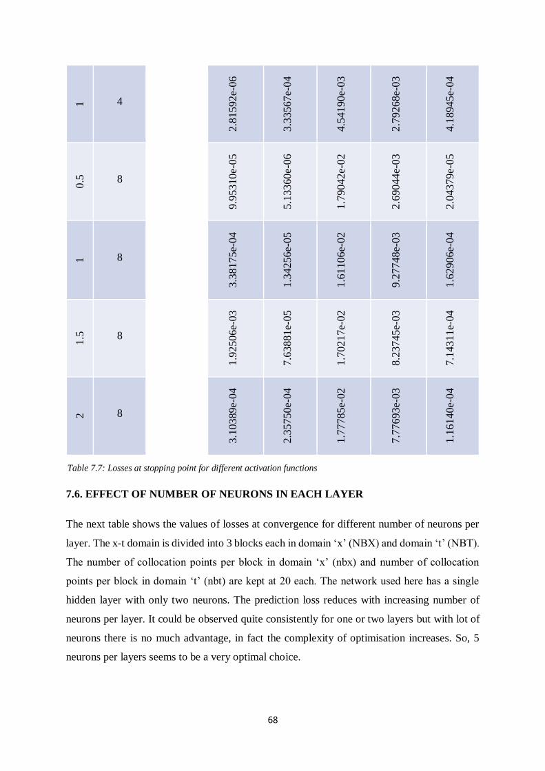
68

1 4

2.8

1592e-

06

3.3

3567e-

04

4.5

4190e-

03

2.7

9268e-

03

4.1

8945e-

04

0.5

8

9.9

5310e-

05

5.1

3360e-

06

1.7

9042e-

02

2.6

9044e-

03

2.0

4379e-

05

1 8

3.3

8175e-

04

1.3

4256e-

05

1.6

1106e-

02

9.2

7748e-

03

1.6

2906e-

04

1.5

8

1.9

2506e-

03

7.6

3881e-

05

1.7

0217e-

02

8.2

3745e-

03

7.1

4311e-

04

2 8

3.1

0389e-

04

2.3

5750e-

04

1.7

7785e-

02

7.7

7693e-

03

1.1

6140e-

04

7.6. EFFECT OF NUMBER OF NEURONS IN EACH LAYER

The next table shows the values of losses at convergence for different number of neurons per

layer. The x-t domain is divided into 3 blocks each in domain ‘x’ (NBX) and domain ‘t’ (NBT).

The number of collocation points per block in domain ‘x’ (nbx) and number of collocation

points per block in domain ‘t’ (nbt) are kept at 20 each. The network used here has a single

hidden layer with only two neurons. The prediction loss reduces with increasing number of

neurons per layer. It could be observed quite consistently for one or two layers but with lot of

neurons there is no much advantage, in fact the complexity of optimisation increases. So, 5

neurons per layers seems to be a very optimal choice.

Table 7.7: Losses at stopping point for different activation functions

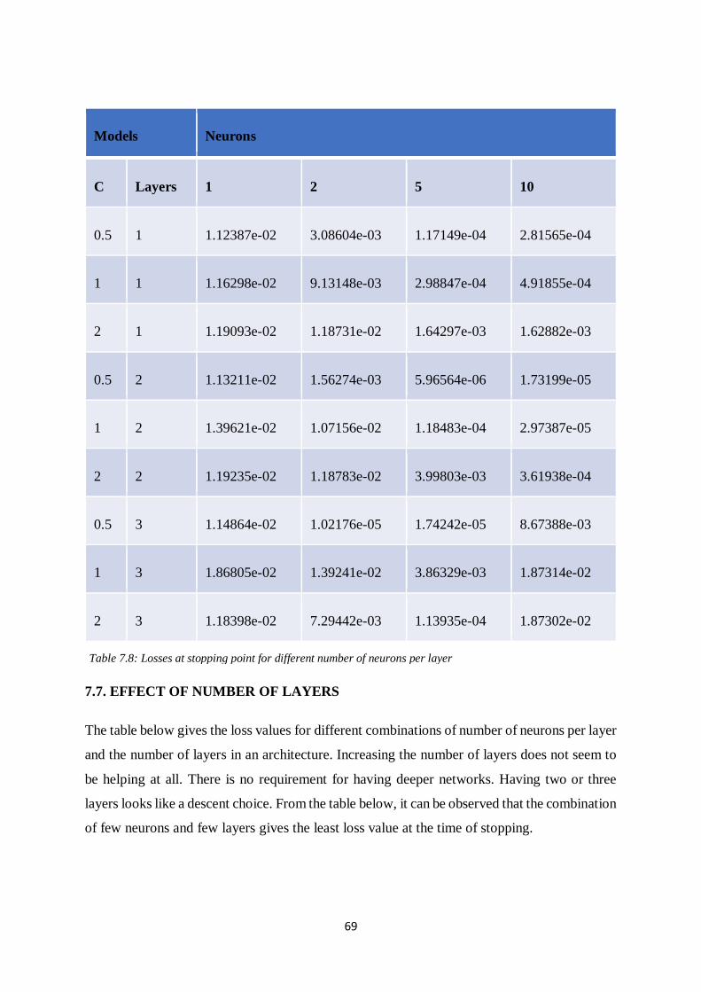
69

Models Neurons

C Layers 1 2 5 10

0.5 1 1.12387e-02 3.08604e-03 1.17149e-04 2.81565e-04

1 1 1.16298e-02 9.13148e-03 2.98847e-04 4.91855e-04

2 1 1.19093e-02 1.18731e-02 1.64297e-03 1.62882e-03

0.5 2 1.13211e-02 1.56274e-03 5.96564e-06 1.73199e-05

1 2 1.39621e-02 1.07156e-02 1.18483e-04 2.97387e-05

2 2 1.19235e-02 1.18783e-02 3.99803e-03 3.61938e-04

0.5 3 1.14864e-02 1.02176e-05 1.74242e-05 8.67388e-03

1 3 1.86805e-02 1.39241e-02 3.86329e-03 1.87314e-02

2 3 1.18398e-02 7.29442e-03 1.13935e-04 1.87302e-02

7.7. EFFECT OF NUMBER OF LAYERS

The table below gives the loss values for different combinations of number of neurons per layer

and the number of layers in an architecture. Increasing the number of layers does not seem to

be helping at all. There is no requirement for having deeper networks. Having two or three

layers looks like a descent choice. From the table below, it can be observed that the combination

of few neurons and few layers gives the least loss value at the time of stopping.

Table 7.8: Losses at stopping point for different number of neurons per layer

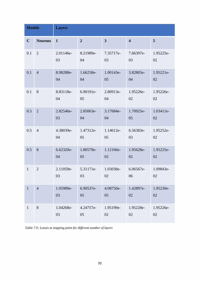
70

Models Layers

C Neurons 1 2 3 4 5

0.1 2 2.01146e-

03

8.21989e-

04

7.35717e-

03

7.66397e-

03

1.95225e-

02

0.1 4 8.98288e-

04

1.66258e-

04

1.00143e-

05

3.82805e-

04

1.95221e-

02

0.1 8 8.83118e-

04

6.90191e-

05

2.80913e-

04

1.95226e-

02

1.95226e-

02

0.5 2 2.82546e-

03

2.85063e-

04

3.17684e-

04

1.70925e-

05

1.03411e-

02

0.5 4 4.38039e-

04

1.47312e-

05

1.14612e-

05

6.56383e-

03

1.95252e-

02

0.5 8 6.62320e-

04

1.80579e-

05

1.12166e-

02

1.95628e-

02

1.95225e-

02

1 2 2.11059e-

03

5.31171e-

03

1.03038e-

02

6.06567e-

06

1.09843e-

02

1 4 1.05989e-

03

6.90537e-

05

4.08750e-

05

1.42897e-

02

1.95230e-

02

1 8 1.04268e-

03

4.24757e-

05

1.95199e-

02

1.95228e-

02

1.95226e-

02

Table 7.9: Losses at stopping point for different number of layers

71

CHAPTER 8

CONCLUSIONS

To summarize, the proposed methods is a good approximation method to solve wide class of

CFD problems. It works much better than the prevalent methods. The older method by I. E.

Lagaris et.al. could solve an advection dominant problem if 𝝐 > 0.5 while the recent version

by Maziar Raissi et. al. could solve a problem if 𝝐 > 0.15. The proposed method Distributed

Physics Informed Neural Network (DPINN) could easily solve the same problem for 𝝐 > 0.002.

The next level advancement, ELM based DPINN, could easily solve for 𝝐 > 0.003 while it

struggles a bit for lower 𝝐 due to large memory involved in the process. In future these methods

can grow up to replace the conventional methods. Otherwise ELM is faster than all the above

model discussed above and gives solution in single shot.

RECOMMENDATIONS FOR THE FUTURE WORK

The problems at current level is the competition with prevalent conventional methods. The

machine learning models generally take time to train themselves so, these models are slower

compared to conventional models. Since, it has been discussed how these models can

overpower conventional methods, there is no doubt on the ability. So, lot of research need to

be done to figure out the solutions.

One method can be to go for adaptive splitting of domains like adaptive meshing in

conventional methods. That would certainly reduce the computational burden.

Another thing that could be researched on is the optimization issue in solving extreme

problems. There should be a method to improve the optimization. One way would be to pose

the various loss objectives together in a better way like assigning proper weights, similar to the

logic behind Lagrange’s multiplier method for multi-objective method.

The solutions for negative 𝝐 are somehow, way better. The reason behind this could be

researched.

The ELM based DPINN fails for larger matrices due to the issue of large memory. A better

method can be proposed to tackle this issue.

72

REFERENCES

[1] G Cybenko, "Approximation by superpositions of a sigmoidal function." Mathematics of

Control, Signals, and Systems (MCSS) 2, no. 4 (1989): 303--314.

[2] Kurt Hornik, Maxwell Stinchcombe and Halbert White, "Multilayer feedforward networks

are universal approximators." Neural Networks 2, no. 5 (1989): 359 - 366.

[3] Isaac E. Lagaris, Aristidis Likas and Dimitrios I. Fotiadis, "Artificial neural networks for

solving ordinary and partial differential equations." IEEE Trans. Neural Networks 9, no. 5

(1998): 987-1000.

[4] Maziar Raissi, Paris Perdikaris and George E. Karniadakis, "Physics Informed Deep

Learning (Part I): Data-driven Solutions of Nonlinear Partial Differential

Equations." CoRR abs/1711.10561 (2017).

[5] Guang-Bin Huang, Qin-Yu Zhu and Chee Kheong Siew, "Extreme learning machine:

Theory and applications." Neurocomputing 70, no. 1-3 (2006): 489-501.