FEDERAL RESERVE BANK OF SAN FRANCISCO

WORKING PAPER SERIES

Monetary and Macroprudential Policy in a Leveraged Economy

Sylvain Leduc

Federal Reserve Bank of San Francisco

Jean-Marc Natal Swiss National Bank

April 2015

Working Paper 2011-15 http://www.frbsf.org/publications/economics/papers/2011/wp11-15bk.pdf

Suggested citation: Leduc, Sylvain and Jen-Marc Natal. 2015. “Monetary and Macroprudential Policy in a Leveraged Economy.” Federal Reserve Bank of San Francisco Working Paper 2011-15. http://www.frbsf.org/economicresearch/publications/working-papers/wp11-15bk.pdf The views in this paper are solely the responsibility of the authors and do not necessarily reflect the views of the International Monetary Fund, its Executive Board, or IMF management, the Federal Reserve Bank of San Francisco or the Board of Governors of the Federal Reserve System.

Monetary and Macroprudential Policy in a Leveraged

Economy ∗

Sylvain Leduc†and Jean-Marc Natal‡

April 2015

Abstract

We examine the optimal monetary policy in the presence of endogenous feedback

loops between asset prices and economic activity. We reconsider this issue in the context

of the financial accelerator model and when macroprudential policies can be pursued.

Absent macroprudential policy, we first show that the optimal monetary policy leans

considerably against movements in asset prices and risk premia. We show that the optimal

policy can be closely approximated and implemented using a speed-limit rule that places

a substantial weight on the growth of financial variables. An endogenous feedback loop is

crucial for this result, and price stability is otherwise quasi-optimal. Similarly, introducing

a simple macroprudential rule that links reserve requirements to credit growth dampens

the endogenous feedback loop, leading the optimal monetary policy to focus on price

stability.

Keywords: Monetary Policy, asset prices, risk premia, price stability

JEL codes: E52,E58,E32,E44

∗The views expressed in this paper are those of the authors and do not necessarily represent the views of

the International Monetary Fund, its Executive Board, or IMF management, the Federal Reserve Bank of San

Francisco, or any other person associated with the Federal Reserve System.†Federal Reserve Bank of San Francisco. Corresponding Author: Sylvain Leduc, Telephone 415-974-3059,

Fax 415-974-2168. Email address: sylvain.leduc@sf.frb.org‡International Monetary Fund. Email address: JNatal@imf.org

1

1 Introduction

The financial crisis of 2007-2009 has led to a reconsideration of the role of financial stability in

the conduct of monetary policy. In particular, the crisis reignited the view that central banks’

focus on inflation targeting may be insufficient to bring about macroeconomic stability and

may need to be complemented with targets for some financial measures such as credit, leverage,

or asset prices. Indeed, many policymakers have acknowledged that the financial crisis has led

them to adjust their views on the role of asset prices in the conduct of monetary policy.1

Nevertheless, in keeping with Tinbergen’s principle of allocating one instrument per tar-

get, the generally preferred approach to tackling financial stability remains to use policy in-

struments specifically designed for the task, such as micro- or macroprudential policies, and let

monetary policy focus on the stabilization of inflation and output gaps.2 Yet, this first-best

strategy may come with important limitations. As Stein (2013, 2014) emphasized, it is unlikely

that macroprudential policies by themselves can perfectly contain an unwarranted rise in lever-

age and credit risk in the economy, partly because macroprudential tools may be difficult to

adjust on a timely basis and partly because they don’t affect all parts of the financial system

equally. In contrast, monetary policy does affect all parts of the financial system (i.e., “it gets

in all of the cracks”) through changes in interest rates and thus the cost of leverage. In this

second-best world, monetary policy could be considered a valuable alternative.

In this paper, we reconsider the role of financial variables in the implementation of mon-

etary policy in the presence of endogenous feedback loops between asset prices, firms’ financial

health, and overall economic activity, using the financial accelerator model of Bernanke, Gertler,

and Gilchrist (1999, BGG). In this framework, entrepreneurs need external sources of funds to

finance investment and their level of net worth affects their cost of capital. By directly affecting

entrepreneurs’ net worth, swings in asset prices affect the cost of credit financing and tend to

amplify movements in investment. In contrast to the work of Bernanke and Gertler (1999, 2001)

and Gilchrist and Leahy (2002), who focused on simple interest rate rules, we emphasize the

1See, for instance, Yellen (2009) who argues that circumstances may develop where it might be appropriateto lean against booming asset prices with tighter monetary policy.

2See Bernanke (2012) among others.

2

design of optimal policy under commitment and study its impact on asset prices and risk pre-

mia (external finance premium, in the words of BGG). To emphasize the issue raised by Stein,

we first assume that macroprudential policies are unavailable to policymakers but that they

may instead rely on monetary policy to address financial stability issues.3 We then introduce

macroprudential policy and examine how the optimal policy prescription is affected.

We first show that when macroprudential policy is unavailable, the optimal monetary

policy deviates significantly from perfect price stability – the canonical New Keynesian bench-

mark – and instead leans considerably against movements in financial variables, such as asset

prices, leverage, risk premia, or credit growth. This reflects the fact that the tightness of firms’

financial constraints varies with the state of the business cycle (a central feature of the financial

accelerator), and that, as a result, so does the degree of inefficiency of natural output, i.e.,

the level of output that ensures perfect price stability. In this context, perfect price stability

is suboptimal. Policymakers lean against swings in financial variables (asset prices, leverage,

and risk premia) because doing so reduces inefficient fluctuations in output. Hence, optimal

policy trades off volatility in the inflation rate for a more efficient allocation of production. In

addition to productivity shocks, we experiment with risk shocks, which have been emphasized

in the literature as an important driver of the business cycle (see Christiano et al., 2014). We

show that the trade-off is more acute when the economy is hit by risk shocks.

Fundamentally, optimal policy leans against movements in financial variables because

the feedback loop gives rise to a pecuniary externality.4 Entrepreneurs do not internalize the

effect of their borrowing behavior on the price of capital and thus on their ability to borrow.

For instance, when entrepreneurs as a group borrow more to buy capital goods, the price of

capital is bid up. Since net worth is positively related to the price of capital, entrepreneurs’

net worth rises, as does their ability to borrow. Because this externality is not internalized by

each individual entrepreneurs, it ultimately leads to overborrowing and inefficient movements

in output.

A second result of the paper is to show that optimal policy can be closely approximated

3Curdia and Woodford (2009) and Woodford (2012), for instance, adopt a similar strategy.4Christiano and Ikeda (2011) discuss the pecuniary externality in the BGG model.

3

by simple “speed-limit” interest rate rules that place a considerable weight on the growth of

financial variables in response to real or financial shocks. These rules have the advantage of

relying solely on observables. They are also relatively easy to implement as they do not require

undue knowledge about the efficient levels of variables, which are typically difficult to assess,

particularly in the case of financial variables.5 We consider a rule that includes the change in the

external finance premium, but our results would be similar if we included alternative measures

such as the changes in equity prices, net worth, the leverage ratio, risk premia, or credit as an

indicator of financial pressure (see, e.g., Stein, 2014 for an emphasis on risk premia). Broadly

speaking, we find that the optimized interest rate rule (the one that best approximates the

allocation under optimal policy) is one that puts substantial weight on inflation and the growth

of financial variables.6

While the suboptimality of perfect price stability policy may be seen as intuitive given

the presence of financial frictions, we show that it hinges on two aspects of the model. First,

it crucially rests on the presence of an endogenous feedback loop between asset prices and

investment – the so-called financial accelerator. When we eliminate the fluctuations in asset

prices by allowing capital to adjust at no cost, we find that the optimal policy closely follows

the standard prescription to stabilize prices, even in the presence of agency costs. Only when

financial fluctuations are significant enough to lead to substantial inefficiency in the equilibrium

allocation does optimal policy mitigate movements in asset prices and other financial variables.

This result points to the importance of incorporating costly capital accumulation in the model

to generate potentially large endogenous movements in asset prices and net worth.

Second, the optimal monetary policy leans against movements in asset prices only when

the financial friction interacts with the monopolistic distortion in steady state. With a positive

steady-state markup, the inefficient movements in economic activity arising from the presence

of agency costs get amplified (for standard nonlinear utility), and the optimal policy trades

5Interest rate rules including a change in asset prices have also been studied by Gilchrist and Saito (2008)in a model with imperfect information, and by Tetlow (2006) under model uncertainty.

6Examining alternative monetary policy rules in the BBG framework in response to financial shocks, Gilchristand Zakrajsek (2012) also find that placing some weight on the external finance premium in a Taylor-type rulebrings about stabilization benefits.

4

off price stability for a more efficient output allocation by leaning against movements in asset

prices and mitigating the effects of the financial accelerator and the associated externality.

When we instead allow for a subsidy that eliminates the positive steady-state markup, as is

often assumed in the literature, we find that the optimal monetary policy is essentially price

stability. Hence a meaningful role for asset prices in the design of optimal monetary policy

emerges only in economies in which the natural and efficient allocations differ markedly.

In the last part of the paper, we introduce macroprudential policy and examine its effect

on the optimal monetary policy response to productivity and financial shocks. The design of

macroprudential policies has attracted a lot of attention recently, and many different policies

have been proposed in the literature such as reserve requirements, capital requirements, limits

on the loan-to-value ratio, and dynamic provisioning, to name only a few. Here we focus on a

countercyclical macroprudential rule that links reserve requirements–a natural instrument in our

theoretical environment–to the growth rate of credit in the economy.7 Credit growth is a logical

focal point for a macroprudential rule given the role of credit in amplifying financial imbalances

in periods leading up to financial crises (see Taylor and Schularick, 2012). Policymakers have

also been stressing credit growth as a key indicator of financial excess. For instance, the Basel

III accord suggests an additional countercyclical capital buffer in periods of above average credit

growth.

In addition, countercyclical reserve requirements have often been used in developing

economies faced with large financial fluctuations (Federico, Vegh, and Vuletin, 2012) and may be

relevant for industrial countries that desire to develop macroprudential tools.8 Along those lines,

Kayshap and Stein (2012) argued for the use of time-varying reserve requirements on short-term

debts to act as a Pigouvian tax on financial institutions engaged in maturity transformation.

That said, the gist our results should apply more generally to other types of macroprudential

policy that limit credit growth.

7We follow Claessens et al. (2014), among others, and classify reserve requirements under the rubric ofmacroprudential policies.

8Using a large dataset of banks in advanced and emerging markets economies, Claessens et al. (2014) showthat macroprudential policies that limit banks’ assets and liabilities, such as reserve requirements, are alsoeffective in limiting credit growth.

5

When our simple macroprudential rule is calibrated to maximize household welfare, bring-

ing about reserve requirements that vary positively with credit growth, we show that the optimal

monetary policy is akin to ensuring perfect price stability since the macroprudential rule damp-

ens the endogenous feedback loop. As credit expands, for instance following an output boom,

reserve requirements increase, dampening the associated increase in asset prices and excessive

rise in investment. In this case, the optimal monetary policy can be approximated by an inter-

est rate feedback rule that solely reacts to movements in the inflation rate and nearly stabilizes

prices.

Overall, macroprudential and monetary policy largely operate as substitutes in our en-

vironment: a tighter (looser) macroprudential policy brings about a looser (tighter) optimal

monetary policy. Our results suggest that even relatively simple rules can go a long way in rein-

ing in the financial accelerator so that monetary policy can focus optimally on price stability.

This is particularly the case when the economy is subject to financial shocks.

The remainder of this paper is organized as follows. Before presenting the main building

blocks of our model in section 2, we briefly review the relevant literature and stress the value

added of our analysis relative to previous contributions. We describe the model’s calibration

before presenting our main results in section 3, emphasizing the importance of endogenous

fluctuations in asset prices. We then discuss a simple and implementable speed-limit rule that

closely approximates the optimal monetary policy and conduct a robustness analysis. Finally,

we examine the introduction of a simple macroprudential policy that positively links reserve

requirements to credit growth and study its implication for the optimal monetary policy.

1.1 Related literature

To better emphasize the importance of endogenous feedback loops for monetary policy, we

deliberately relied on a standard model and a standard calibration. In addition to being simple,

this approach has the added benefit of clarifying the paper’s contribution relative to the previous

literature. In particular, by modeling endogenous feedback loops through capital accumulation,

our analysis of optimal policy complements the recent contributions of Curdia and Woodford

6

(2009), Woodford (2012), and particularly those of De Fiore and Tristani (2013), De Fiore,

Teles, and Tristani (2011) and Carlstrom, Fuerst, and Paustian (2010). De Fiore and Tristani

(2013) study the optimal monetary policy in a model with costly state verification and price

rigidity, but one in which there are no endogenous movements in net worth, partly reflecting the

absence of capital accumulation. They derive the loss function of the central bank, which they

show to depend on the volatility of the nominal interest rate and credit spreads, in addition

to the volatility of inflation and that of the output gap. They find that following a financial

shock, interest rates should be aggressively lowered but price stability remains nearly optimal

otherwise.

In contrast, Carlstrom, Fuerst, and Paustian (2010) derive the optimal monetary policy

in an environment in which firms’ labor hiring is constrained by their net worth, as in the

model of Kiyotaki and Moore (1997). They show that the central bank’s loss function is partly

a function of the tightness of the credit constraint, which they interpret as a risk premium.

Although their model abstracts from capital accumulation, it captures endogenous movements

in net worth through movements in share prices of monopolistic sticky-price firms. They show

that stabilizing inflation is nearly optimal in their framework, even if the credit constraint is

quite severe, because the weight on inflation volatility in the central bank’s loss function dwarfs

that on the variability of the risk premium.

De Fiore, Teles, and Tristani (2011) also examine the optimal monetary policy in a

model with agency costs in which firms’ financing conditions are predetermined. They show

that the optimal policy allows deviations from price stability to mitigate output fluctuations

via movements in firms’ real funds needed to finance production.

One important distinguishing feature of our work is the introduction of capital accumu-

lation, which allows us to directly examine the importance of the financial accelerator for the

design of optimal monetary policy. This additional feature allows an endogenous feedback be-

tween asset prices, net worth, and economic activity, which implies that the optimal monetary

policy should lean against movements in financial variables,bringing about departures from

perfect price stability. Absent this mechanism, price stability is quasi-optimal.

7

Our paper also relates to Faia and Monacelli (2007), who study the design of optimized

interest rate rules in response to technology and government spending shocks in a model with

agency costs adapted from the work of Carlstrom and Fuerst (1997). Faia and Monacelli

find that the optimal rule remains focused on stabilizing inflation. One important difference

between our analysis and theirs is that we explicitly consider a model where the efficient and

natural output differ markedly. We also complement their analysis by emphasizing the design

of optimal policies under financial shocks and by considering speed-limit rules as implementable

policy rules.

Finally, we add to this body of work by considering the impact of simple macroprudential

rules on the optimal monetary policy. In so doing, our paper also complements a growing

body of work that examines the effects of different macroprudential policies on the economy

(see Christensen, Meh, and Moran (2011), Angeloni and Faia (2013), and Quint and Rabanal

(2013), among others). To keep our analysis tractable we abstracted from modeling the strategic

interactions between monetary and macroprudential policies. However, benefits can arise from

policy coordination (on this issue see, for instance, Beau, Clerc, and Mojon (2011), Collard et

al. (2012) and Angelini, Neri, and Panetta (2014)).

2 The model

Our analysis draws on BGG’s seminal work and on the more recent contributions of Christiano,

Motto, and Rostagno (CMR (2003, 2010, 2014)). The economy consists of four sectors. The

first two sectors produce intermediate and final goods, respectively, while the third produces

physical capital and the fourth provides loans to investors and can be interpreted as a pseudo-

banking sector. Banks in our framework are risk-averse and hold a perfectly diversified portfolio

of entrepreneurial loans. The economy is populated by households composed of consumers and

workers and by risk-neutral entrepreneurs. The latter own the capital stock and provide capital

services to intermediate goods producers. Entrepreneurs finance their purchases of capital

both with internal funds (own net worth) and external funds (bank loans). Entrepreneurs

face idiosyncratic productivity shocks and are subject to bankruptcy if their project fails. The

8

banking sector receives deposits from households (which are considered riskless and are thus

remunerated as such) and make loans to entrepreneurs. A key mechanism of the model is that

the premium over the risk-free rate – the so-called external finance premium – that entrepreneurs

must pay to borrow is related to their leverage. The more “skin in the game” the entrepreneurs

have, the smaller is the moral hazard problem and the premium.

In the following, we describe the main building blocks of the model, which features a

traditional New Keynesian model augmented by a financial accelerator following BGG and

CMR. More details can be found in the appendix.

2.1 Main building blocks

2.1.1 Capital producers

As in CMR (2010, 2014), there is a large number of identical capital producers operating under

perfect competition who, at time t, produce new physical capital kt+1 to be used in t+ 1, using

the following production function:

kt+1 = (1− δ) kt + (1− S (it/it−1)) it,

where it denotes investment, δ is the depreciation rate 0 ≤ δ ≤ 1 and S (·) is an increasing

and convex function. The new capital stock is sold at price Qt and the old capital stock is

purchased at price Qt on the capital market. Therefore, profits are given by

Πkt = Qtkt+1 − Ptit − Qtkt.

Maximizing profit subject to the production constraint leads to the following two first-

order conditions:

Qt ((1− S (it/it−1))− S ′ (it/it−1) it/it−1) = Pt (1)

Qt = Qt (1− δ) . (2)

9

2.1.2 Entrepreneurs

There is a large number of heterogeneous entrepreneurs, indexed by j, who buy new capital

stock kj,t+1 at price Qt from the capital producers and transform it into capital services xj,t+1

according to the linear technology:

xj,t+1 = ωjkj,t+1, (3)

where ωj denotes the productivity of the transformation technology which is entrepreneur-

specific. The random variable ω is drawn from a cumulative distribution denoted by Ft(ω?) =

P (ωj 6 ω?) with mean E(ω) = 1. Entrepreneurial investment is risky and, as in CMR, the

degree of risk is assumed to vary over time. Therefore we assume that log(ω) is normally

distributed with mean µω,t and standard deviation σω,t. The standard deviation σω,t is the

realization of a mean-preserving stochastic process referred to below as a “risk shock,” which

follows an AR(1) process with autoregressive coefficient ρσω and innovations, εσω , assumed to

be normally distributed with mean zero and standard deviation σεσω .

Each entrepreneur draws its type ωj after capital kj,t+1 has been purchased. To purchase

capital, each entrepreneur can either use her net worth Nj,t+1 or borrow Bj,t+1 from banks at the

gross rate of interest Rbj,t+1. To ensure that entrepreneurs do not accumulate enough net worth

to make the borrowing constraint nonbinding, we assume that entrepreneurs exit the economy

(close business) each period with probability 1 − γ.9 Within each period, entrepreneurs rent

their capital services to intermediate goods producers at the real price zt+1, and at the end of

the period they resell their capital stock to capital producers at price Qt+1.

Hence, entrepreneur j’s expected revenue from purchasing capital can be written as

Et

[Pt+1zt+1ωjkj,t+1 + Qt+1ωjkj,t+1

].

Denoting the rate of return on capital as

Rkt+1 ≡

Pt+1zt+1 + Qt+1

Qt

,

9To maintain a constant population of entrepreneurs, we assume that 1 − γ new entrepreneurs are born atthe same time. These entrepreneurs finance their purchases with a transfer, τet , that they receive from thegovernment. Departing entrepreneurs consume their net worth.

10

we can rewrite an entrepreneur’s expected revenue in the following way

Et[QtR

kt+1ωjkj,t+1

]. (4)

To finance capital purchases, the entrepreneur can either use her net worth Nj,t+1 or enter a

contract with a bank to borrow Bj,t+1 at gross rate Rbj,t+1, such that

Qtkj,t+1 = Nj,t+1 +Bj,t+1.

The debt contract then specifies the loan amount Bj,t+1 and the nominal gross rate Rbj,t+1. If

the entrepreneur’s project is a success she pays back the loan and interest (Rbj,t+1Bj,t+1) to the

bank. If the project fails (because the project’s productivity, ωj, turns out to be too low) the

bank pays a proportional cost µ to monitor the entrepreneur and confiscates the remaining

assets. Thus, there exists a cutoff value ω?j,t+1 defined as

Rbj,t+1Bj,t+1 = ω?j,t+1QtR

kt+1kj,t+1 (5)

below which the entrepreneur declares bankruptcy.

The expression for an entrepreneur’s expected profit can be derived to be

Et

[∫ ∞ω?j,t+1

(ωQtRkt+1kj,t+1 −Rb

j,t+1Bj,t+1)dF (ω)

].

Using the definition of the cutoff value ω?j,t+1, and making use of the fact that kj,t+1 is decided

in period t, the expected profit function rewrites as

Et

[∫ ∞ω?j,t+1

(ω − ω?j,t+1)Rkt+1dF (ω)

]Qtkj,t+1, (6)

which defines the entrepreneur’s objective function.

2.1.3 Banks and reserve requirements

Since the bank receives Rbj,t+1Bj,t+1 if an entrepreneur’s productivity is higher than the cutoff

value ω?j,t+1 and otherwise seizes all the entrepreneur’s assets ωjQtRkt+1kj,t+1 if the project fails

(after having paid a proportional monitoring cost, µ), the bank’s revenue corresponds to:∫ ∞ω?j,t+1

Rbj,t+1Bj,t+1dF (ω) + (1− µ)

∫ ω?j,t+1

0

ωQtRkt+1kj,t+1dF (ω)

11

which can be rewritten as

(1− F (ω?j,t+1))Rbj,t+1Bj,t+1 + (1− µ)

∫ ω?j,t+1

0

ωQtRkt+1kj,t+1dF (ω).

Banks are assumed to be perfectly competitive and riskless. They finance themselves via

household deposits Bj,t+1 that earn the nominal (risk-free) gross interest rate Rt, where Rt is

not contingent on shocks realized in t+ 1.

In addition, banks’ lending is subject to macroprudential policy restrictions. In particular,

we assume that banks are subject to a reserve requirement, φt, which varies with indicators of

financial activity, FIt, (for instance, credit growth, leverage ratio, asset prices, among others)

according to a simple rule

φt = φ∗ + χFIt, 0 < φt < 1 (7)

where φ∗ is a constant and χ is a parameter calibrated such that 0 < φt < 1 for reasonable

values of FIt.

For simplicity, banks’ reserves are assumed to be kept in “cash” and earn a zero rate

of return.10 Given the reserve requirement, φt, determining the fraction of loanable deposits,

the financial intermediary must issue Bj,t+1/(1 − φt) deposits to finance Bj,t+1 loans per en-

trepreneurs. Therefore, the zero profit condition implies

(1− F (ω?j,t+1))Rbj,t+1Bj,t+1 + (1− µ)

∫ ω?j,t+1

0

ωQtRkt+1kj,t+1dF (ω) = Rt

Bj,t+1

(1− φt), (8)

which also corresponds to the bank’s participation constraint.

In turn, the contract between a bank and a borrower specifies a level of loans, Bj,t+1 and a

gross interest rate Rbj,t+1 that maximizes the expected profit of the entrepreneur, subject to the

participation constraint of the bank. Equivalently the contract determines a level of capital,

kj,t+1, and a cutoff point, ω?j,t+1 by maximizing entrepreneurs’ profits, subject to the bank’s

10We could alternatively assume that reserves are remunerated. The key assumption is that the rate of returnon reserves should be smaller than the rate Rt earned by households on bank deposits such that an increase inreserves leads to an increase in the risk premium, as per the banks’ zero profit condition.

12

participation constraint above. In the appendix, we show that the solution to this problem is

given by the following two equations

Et

[[1− Γ(ω?j,t+1)

]Rkt+1 +

[Γ(ω?j,t+1)− µG(ω?j,t+1)

]Rkt+1 − Rt

(1−φt)

1− µω?j,t+1h(ω?j,t+1)

]= 0 (9)

[(Γ(ω?j,t+1))− µG(ω?j,t+1)

]QtR

kt+1kj,t+1 −Rt

(Qtkj,t+1 −Nj,t+1)

(1− φt)= 0. (10)

Note that the presence of reserve requirements, φt, affects the contract between the bank and

the entrepreneur. In Section 3.6 below, we show that a tighter macroprudential policy captured

by a higher reserve requirement, φt, leads to a higher spread between the risky and riskless rates

of return. Intuitively, since part of the bank’s source of funds must be held in reserve, it is

more costly for the bank to make a loan of a given size, which is reflected in a higher interest

rate spread.11 Clearly, the standard contract arises in the absence of reserve requirements (i.e.,

φt=0, for all t).

2.1.4 Aggregated net worth

The contract between a bank and an entrepreneur specifies a level of loans, Bj,t+1, and a gross

interest rate, Rbj,t+1, that maximizes the expected profit of the entrepreneur subject to the

bank’s participation constraint, or identically a level of capital kj,t+1 and a cutoff point ω?j,t+1.

Clearly, the amount of loans and therefore the level of investment will depend on entrepreneurs’

net worth Nj,t+1 (the new state variable associated with asymmetric information). Aggregating

over all entrepreneurs, it can be shown (see Appendix and BGG for details) that entrepreneurial

net worth evolves according to

Nt+1 = γΞt + τ et ,

where Ξt is the aggregate profit flow to entrepreneurs, τ et is the government transfer to “newly

born” entrepreneurs, and γ is the entrepreneurs’ constant survival probability.12

11Quint and Rabanal (2011) also introduce a macroprudential regulation in a financial accelerator model ofa monetary union, which increases the spread faced by borrowers.

12In Leduc and Natal (2011), we also examined a shock to net worth, as captured by an innovation to γt.

13

2.1.5 Intermediate goods producers

Intermediate goods producers are monopolistically competitive. They produce an intermediate

good by means of capital and labor according to a constant return to scale production function:

yt (i) = atkt (i)α ht (i)1−α with α ∈ (0, 1) , (11)

where kt (i) and ht (i) respectively denote the physical capital and the labor input used by

firm i to produce yt (i), and where at represents total factor productivity, which is assumed to

follow an AR(1) process with autoregressive coefficient ρa and innovation, εa, that is normally

distributed with mean zero and standard deviation σa.

The firm determines its production plan to minimize its total cost :

min{ht(i),kt(i)}

Ptwtht(i) + Ptztkt (i)

subject to production. As is standard in the New Keynesian literature, we assume that firms

set their prices according to Calvo’s staggering scheme and define τ as the probability that a

particular firm is able to reset its price next period.

2.1.6 Final goods producers

Final goods are produced by competitive retailers that assemble intermediate goods according

to a CES aggregator

yt =

(∫ 1

0

yt (i)1λ di

)λwith λ ∈ [1,∞),

where λ stands for the elasticity of substitution between intermediate goods and determines

the intermediate good producers’ market power (or the steady-state markup of price P over

their marginal costs).

2.1.7 Households

The representative household maximizes the discounted value of its lifetime utility that features

preferences over consumption and labor:

Ut = E0

∞∑j=0

βj(

1

1− σcc1−σct+j −

νh1 + σh

h1+σht+j

), (12)

14

subject to the budget constraint

PtCt = Ptwtht + Πt +Rt−1Bt −Bt+1,

where Πt represents the dividends earned on the profits of intermediate goods firms, 0 < β < 1

represents the rate of time preference, and νh is a normalizing constant.

The household is also subject to the time endowment constraint

lt + ht = 1,

where lt denotes the proportion of total time dedicated to leisure.

2.2 Baseline calibration

The baseline calibration is standard and is reported in Table 1. We assume a coefficient of

relative risk aversion, σc = 1.5 and we set σh to 1, implying a unit Frisch elasticity of labor

supply. We choose β=0.99, leading to an annual real interest rate of 4 percent.

Because of monopolistic competition and costly state verification (the model’s financial

friction for µ > 0), the steady state of the model is distorted. The gross markup of price over

marginal costs, λ, is set to 1.1. The capital share parameter in the Cobb-Douglas production

function α = 0.36, and the quarterly depreciation rate is 2.5 percent per quarter. We assume

a Calvo parameter θ of 0.75, so that, on average, firms expect to be able to change their price

once a year.

We follow BGG (1999), Carlstrom and Fuerst (1997), and CMR (2010), and calibrate

the financial intermediation block to obtain an annual credit risk premium (Rk

R) of about 2

percentage points in the steady state. The entrepreneur’s ex ante survival probability (from

one quarter to the next), γ, is set to 97.28 percent, in line with BGG. We set the bank’s

monitoring cost as a share of final output, µ = 0.2 while F (ω?), the proportion of businesses

going bankrupt per quarter, is set to 0.75 percent.

Those parameter values imply the economy’s steady-state capital-output ratio, ky

= 8.08

and the investment-output ratio, iy

= 0.2 , broadly in line with estimations provided by CMR

(2010) for the euro area (8.70; 0.21) and the United States (6.98; 0.25).

15

We specify the investment adjustment cost function as in CMR (2014):

S(xt) =1

2

{exp

[√S ′′(xt − x)

]+ exp

[−√S ′′(xt − x)

]− 2}, (13)

where xt ≡ it/it−1 and x represents its steady-state value. Note that S(x) = S ′(x) = 0 and

S ′′(x) = S ′′, where S ′′ is a model parameter that we calibrate to 10, based on the estimated

value in CMR (2014).

As mentioned previously, our macroprudential policy takes the form of a reserve require-

ment rule given by equation (7) above and reproduced here for convenience

φt = φ∗ + χFIt, 0 < φt < 1.

In the benchmark model, we first abstract from macroprudential policy and set φ∗ = χ = 0. For

the experiments in which we introduce macroprudential policy, we first set φ∗ in line with the

evidence in Federico, Vegh, and Vuletin (2012) who find that the average reserve requirement

in industrialized countries over the period 1975-2011 is 2 percent. We then consider a reserve

requirement rule in which the financial indicator is credit growth. We first concentrate on an

optimized value of χ. Specifically, we find the value of χ that maximizes welfare, assuming that

monetary policy is set optimally taking into account the macroprudential rule (we describe the

way we characterize the optimal monetary policy below). This leads to χ = 1.0064, so that

reserve requirements vary positively with credit growth (i.e., they are countercyclical). We then

compare this rule’s implications to one where reserve requirement respond more aggressively to

credit growth, setting χ = 3.13

Finally, in all the simulation exercises, we set the parameters (ρa, ρσω and σεa , σεσω ) of

the AR(1) processes to correspond to the mode of their estimated posterior distribution for the

United States in CMR (2014).

13Assuming that monetary policy pursues strict price stability, for instance, we find an optimal value ofψ = 1.85.

16

3 The results

We compute the optimal monetary policy under commitment following the timeless perspective

approach of Woodford (2003). We do so explicitly by acknowledging the distorted nature of the

steady state. That is, competitive inefficiencies are not offset by lump-sum subsidies (see, for

instance, Benigno and Woodford, 2005) and monitoring costs are positive in the steady state.

We study the responses to shocks to aggregate productivity, at, and to the cross-sectional distri-

bution of entrepreneurs’ individual productivity, σω, and contrast the optimal precommitment

policy to the traditional New Keynesian optimal benchmark, which consists of ensuring perfect

price stability.

As a useful and simpler benchmark, we first abstract from macroprudential policies,

setting φt = 0, for all t. Using this benchmark model, we show three main results. First, the

presence of a financial accelerator introduces a nontrivial policy trade-off that is especially acute

in response to financial shocks. Endogenous fluctuations in net worth triggered by fluctuations

in asset prices play an important role in driving resource allocation away from their most efficient

use. This is in contrast to a recent literature (e.g., Faia and Monacelli (2007)) that finds that

the traditional New Keynesian optimal policy prescription (perfectly stabilizing prices under

both real and financial shocks) remains optimal even in the presence of financial frictions.

Second, we show that the large consensus around a policy of perfect price stabilization,

even in the presence of a financial accelerator, is due to the standard (and unrealistic) New Key-

nesian assumption that policymakers can compensate workers for the monopolistic competition

distortion in a lump-sum fashion. While the financial friction is a necessary condition for a

policy trade-off to arise, the latter remains quantitatively small if the competitive distortion–by

far the largest friction in the model–is subsidized away.14

Third, to study the importance of asset prices, interest rate spreads, or leverage ratio

targeting in the conduct of monetary policy, we simulate the economy under different interest

rate rules to which we append these alternative indicators. We show that the optimal precom-

14In Leduc and Natal (2011), we show that the optimal policy prescription is invariant to whether householdbank deposits are protected against surprise inflation (as in BGG 1999) or not (as in CMR 2010).

17

mitment policy can be closely approximated and implemented using a speed-limit monetary

policy rule that places a substantial weight on the growth rate of financial variables.

We then modify this benchmark model by introducing a simple, implementable, macro-

prudential policy with countercyclical reserve requirements (where reserve requirements increase

with credit growth). Introducing this simple rule has a substantial impact on our benchmark

result. When the macroprudential policy leans against credit growth, the optimal monetary

policy focuses almost exclusively on price stability in response to productivity and financial

shocks. Hence, the macroprudential and monetary policies are substitutes: a tighter (looser)

macroprudential policy brings about a looser (tighter) optimal monetary policy.

3.1 Optimal monetary policy

Following Woodford’s (2003) timeless perspective approach, impulse responses under optimal

policy refer to an equilibrium where policy is described by the first-order conditions of a Ramsey

planner deciding on allocation for t ≥ 1 and ignoring the potential time inconsistency problem

due to the particular nature of t = 0. Dynare is used to solve for optimal policy.

In the BGG framework, optimal policy is difficult to characterize since, in principle, the

social planner has to maximize welfare of two different types of agents, households and en-

trepreneurs. This is nontrivial since entrepreneurs and households have different degrees of risk

aversion (entrepreneurs are risk-neutral) and different discount factors. In BGG, entrepreneurs

are assumed to be extremely patient since they are willing to postpone consumption to the

period before they die.

Following De Fiore et al. (2011), we do not include the entrepreneurs in the social

welfare function because we do not want to think of them as actual agents but as a way to

introduce the financial friction in the model. Moreover, because entrepreneurs are risk-neutral,

the volatility of the economy under different policies does not affect the entrepreneurs’ average

level of consumption. Therefore, excluding entrepreneurs from the welfare calculation does not

impact the welfare ranking of alternative policies, as it would only introduce a constant in the

welfare calculation (see Faia and Monacelli 2007 for a similar argument).

18

3.2 Optimal policy versus perfect price stability (PPS)

Consider first the impact of a positive and temporary productivity shock when monetary policy

either is conducted optimally or targets price stability.15 In the financial accelerator model,

higher productivity leads to higher asset prices, which increases entrepreneurs’ net worth and

results in higher investment. In turn, the increase in investment and output stimulates asset

prices, which then feed back into higher net worth and investment. Figure 1 shows that optimal

policy tends to dampen the response of the economy compared to a policy of perfect price

stability (PPS), the canonical New Keynesian benchmark. Compared to PPS, the optimal

policy is more restrictive, as shown by the increase in the real interest rate, which initially

slows the economy and leads to a decline in inflation. On impact the rise of asset prices under

the optimal policy is almost half of that under PPS, which in turn dampens the responses of net

worth, leverage, and the risk premium by similar magnitudes. At the same time, optimal policy

allows some fluctuations in the inflation rate as policymakers trade off inflation stabilization

for output stabilization.

The optimal policy trade-off illustrated in Figure 1 means that there is an externality as-

sociated with the financial accelerator mechanism: The financial friction (monitoring cost) gives

rise to an overreaction of investment and output with respect to the efficient allocation, which

optimal policy takes into account. Figure 2 compares the efficient responses to the responses

that would arise under either PPS or the optimal policy following a positive productivity shock.

We define the efficient response as that of the economy without financial frictions, in which a

lump-sum tax-financed subsidy offsets the monopolistic competition distortion in the steady

state and where prices are perfectly flexible. The figure shows that, under the optimal policy

the rise in net worth and equity is more muted than under the natural allocation brought about

by PPS. Fewer investment projects are financed, which aligns the response of the economy more

closely with the efficient allocation where financial frictions are absent.

Although the difference between the optimal monetary policy and a policy that aims at

15Note that because we assume a non-efficient steady state, the natural allocation ensuring price stability isnot necessarily efficient.

19

PPS remains relatively small following a productivity shock, the departure from price stability

becomes much more pronounced when the economy is hit by financial shocks. Because financial

shocks interfere directly with the financial intermediation process, they have a more direct

bearing on asset prices, net worth, and finance premia than productivity shocks. We examine

a drop in σω, i.e., a decline in the cross-sectional distribution of entrepreneurs’ individual

productivity, interpreted as a decrease in the perception of market risk, which affects risk

premia directly (see CMR (2010)).16 As in the case of a productivity shock, the optimal

monetary policy leans against movements in asset prices and net worth, but the difference

between optimal policy and PPS is somewhat starker. As shown in Figure 3, the optimal

policy is more restrictive than PPS – as reflected in the sudden more pronounced tightening of

real interest rates – dampening the rise in equity prices and avoiding the increase in net worth

that occurs under PPS. By leaning against the jump in asset prices, the optimal policy avoids

the investment spree that characterizes the allocation under PPS, but this requires a temporary

drop in inflation and a more pronounced initial output contraction.17

Interestingly, since optimal policy prevents an increase in entrepreneurs’ net worth, lever-

age (not shown) is higher than under PPS despite lower investment.18 This reflects the fact

that banks are perfectly safe in the model (risk is perfectly diversified), and thus there is no

concern about the extent of leverage in the economy. Optimal policy limits the amplitude of in-

vestment fluctuations that arise out of the financial accelerator’s externality by leaning against

asset prices.

16The analysis is almost isomorphic for shocks to net worth (or γ-shocks) that are central to the analysis inGilchrist and Leahy (2002). However, as explained in CMR (2010), these shocks have counterfactual implicationsfor credit growth and are therefore less likely to be primary drivers of the business cycle. A description of theeffects of shocks to net worth on the economy can be found in Leduc and Natal (2011).

17In Leduc and Natal (2011), we also considered a shock to net worth, as in Gilchrist and Leahy (2002). Asfor a negative σω-shock, the shock to net worth boosts asset prices, investment, and output. We showed that,in this case as well, optimal policy tends to dampen movements in asset prices, net worth, and finance premiacompared to PPS.

18Under our calibration, optimal policy actually engineers a decrease in net worth.

20

3.3 The role of the financial friction and asset prices

How important are movements in asset prices in determining the optimal monetary response?

To isolate the effect of fluctuations in asset prices via the financial accelerator, we trim down

the investment adjustment cost in equation (13). Mechanically, when changing investment is

not costly, asset prices (Tobin’s Q) do not need to increase by much to induce the required

level of investment; in our example, asset prices remain almost fixed. Figure 4 shows the

response of the economy to a positive productivity shock (at) and to a drop in risk (σω,t). It

shows these responses under the optimal policy and price stability in the presence of investment

adjustment costs (our benchmark case) and also under the optimal policy when investment can

be freely adjusted, so that the asset price transmission channel is shut off. The figure shows

that endogenous fluctuations in asset prices and their impact on net worth are first order in

determining the optimal monetary response to shocks. When asset prices do not move, the

optimal policy response to a productivity shock, for instance, is virtually identical to a policy

targeting price stability, as the wedge between natural and efficient output remains almost

constant, an issue we discuss in more detail below. The optimal policy response to the financial

shock becomes also closer to price stability absent fluctuations in asset prices.

What is the importance of the model’s financial friction in driving this result? Figure

5 contrasts the output and inflation responses under the optimal policy for different degrees

of the financial friction. When financial frictions are nearly shut off (setting the monitoring

cost µ = 0.05), PPS is close to optimal following a productivity shock, as movement in asset

prices are muted due to the weak financial accelerator. Similarly, following a financial shock

the movements in output and inflation are somewhat muted when the size of the financial

friction is reduced.19 This result again highlights the importance of the multiplier effects of

asset prices on investment, i.e., the feedback loop through which an increase in asset prices

boosts investment via a rise in net worth and a corresponding drop in the external finance

premium. This dynamic effect pushes the economy to deviate substantially from the efficient

19In terms of financial shocks, Figure 4 and 5 only report the responses to a σω shock, but the responses toa γ shock would tell a similar story.

21

allocation, and price stability is not the welfare-maximizing solution.

3.4 The role of the subsidized steady state

Most authors routinely assume that the government is able to levy a lump-sum tax and transfer

the proceeds to workers in the form of an employment subsidy that compensates them for

the welfare loss associated with the steady-state monopolistic competition distortion. This

assumption makes the equilibrium under flexible prices efficient and, under certain conditions

(see Woodford 2003), optimal monetary policy delivers the flexible price allocation (or constant

markups and prices), which features PPS. Although this assumption is innocuous in a canonical

New Keynesian model where the only other distortion is price stickiness (since the wedge

between efficient and natural output is constant), it can have important consequences when

the economy is simultaneously subject to another real friction, like the countercyclical credit

market imperfections inherent to the financial accelerator model.

In general, the flexible price allocation does not maximize household welfare when there

is a nontrivial real friction and when the steady-state markup is non-zero.20 As shown in Galı,

Gertler, and Lopez-Salido (2007), the welfare loss from output fluctuations is increasing in the

amount of steady-state distortion. In the case of a subsidized steady state, the welfare loss

associated with inefficient output variations is dwarfed by the welfare cost of inflation, and

price stability may remain the welfare-maximizing policy. Figure 6 shows that, indeed, the

optimal policy responses to a productivity shock and to a drop in σω are extremely close to

PPS when a subsidy is available to offset the steady-state monopolistic competition distortion,

even in the presence of financial frictions (µ = 0.2). This result corroborates similar analysis

by Carlstrom, Fuerst, and Paustian (2009) and Faia and Monacelli (2007).

In the financial accelerator model, a positive steady-state markup distortion is important

because it results in a nonconstant wedge between the natural and optimal output response

to shocks. As a result, welfare can be improved by deviating from price stability: trading

20See Adao, Correia, and Teles (2003) for a formal analysis in the context of a monetary model with cash-in-advance constraints and firms that set prices one period in advance. Natal (2012) show that the flexibleprice allocation is not optimal either in models where oil enters as an imperfect substitute for other productionfactors and consumption goods.

22

off some output variability against movements in inflation. Figure 7 shows that the larger

the steady-state markup distortion, the larger is the variability of the wedge, and the larger

the monetary policy trade-off. When the monopolistic distortion is subsidized away, there is

essentially no trade-off , even if the steady state remains inefficient due to the presence of agency

costs. Implicitly, agency costs induce suboptimal output fluctuations that are outweighed by

the costs of inflation fluctuations.21

3.5 Implementing optimal policy

One problem with welfare-based optimal policies is their reliance on unobservables such as the

efficient level of output or various shadow prices, which, in practice, makes them difficult to

implement. A straightforward alternative is to rely on simple but suboptimal rules that are

functions of observables only. Previous literature (see Walsh, 2003) has shown that the optimal

precommitment monetary policy rule can be approximated by a simple inertial policy rule – or

speed-limit rule – in the New Keynesian context. In particular, just as optimal policies with

commitment, a speed-limit rule introduces inertia in output and inflation that would otherwise

be absent with other level-based simple rules. To take into account the extra friction due to

the financial accelerator, we append a financial variable to the rule and postulate the following

general specification:

rt = gππy,t + g∆y (yt − yt−1) + g∆f

(f it − f it−1

), (14)

where variables with a hat denote deviations from the steady state and f it is our financial

indicator. We consider a rule in which we set this indicator to equal the external finance

premium. However, our results are robust to alternative measures such as equity prices, net

worth, or loans because they are all interrelated via the optimal debt contract between banks

and entrepreneurs. The general rule relies on a reasonable information set as only the growth

rates of the variables are required. Using equation (14), we search for the simple rule (over

the space of parameters gπ, g∆y, and g∆f ) that best approximates the optimal precommitment

21Note that this result holds even for larger than one-standard-deviation shocks.

23

plan. To do so, we simply maximize the economy’s social welfare function using a second-order

approximation to the economy’s equilibrium conditions and welfare function.22

Figures 8 and 9 show impulse responses to a productivity shock, at, and a risk shock,

σω, under the optimal plan, the optimized speed-limit rule, and a traditional Taylor rule. The

first part of Table 2 reports the value of the parameters of the optimized rule for the different

exercises using our benchmark model ignoring macroprudential policy.23 The optimized rule

leans strongly against inflation (because of the price friction) and the change in risk premium

(because of the financial friction), but does not react to the change in output (g∆y = 0).

Moreover, the financial friction is quantitatively important and leads the monetary authority

to place a very large weight on the growth in the equity finance premium. Figures 8 and

9 show that our speed-limit rule reproduces very closely the allocation generated under the

optimal policy and particularly leads to inertial, hump-shaped movements in many variables.

In contrast, the standard Taylor rule often misses on the magnitude, and sometimes on the sign,

of the variables’ responses under the optimal policy and typically doesn’t generate hump-shaped

movements.

The importance of leaning against changes in financial variables is highlighted in Figure

10, which compares the responses to each shock when the weight on the growth of the financial

indicator in the speed-limit rule is reduced compared to that in the optimized rule. The

figure shows that a larger weight on the change in fit helps create more inertial responses,

particularly for investment and output. When the policymaker leans less against changes in the

risk premium, investment responds too much too quickly, which leads to suboptimal movements

in consumption (not shown) and output. Strikingly, even relatively modest responses to changes

in fit produce results that are pretty close to the optimized policy.

As a final exercise, we also searched for the parameters of the speed-limit rule that best

match the optimal plan when the two shocks are considered simultaneously. The result, shown

22See also Benigno and Woodford (2005) and Dennis (1999) for discussions of the importance of taking asecond-order approximation to the model solution and issues with the linear-quadratic approach.

23Note also that similar results would be obtained with rules that lean against other financial variables suchas equity prices, net worth, or loans because they are all interrelated via the optimal debt contract betweenbanks and entrepreneurs.

24

in the last row of Table 2, is qualitatively similar to the individual shock exercises presented in

Figures 8 and 9.

Overall, we take from this exercise that, absent macroprudential policy, a speed-limit rule

with a substantial weight on inflation and on the change in the risk premium does a good job

at mimicking the optimal plan. While the optimized weight on the financial variable is rather

large, we take this particular value literally. Indeed, Figure 10 shows that even a significantly

smaller weight on the change in the risk premium goes a long way in approximating the optimal

monetary policy.

3.6 Macroprudential Policy

In this section, we introduce macroprudential policy and study how it impacts the optimal

monetary policy in the benchmark model. In particular, we examine a simple, implementable,

rule that positively links reserve requirements to changes in credit growth. We focus on credit

growth since the literature has emphasized this variable as a useful indicator of financial im-

balances (see, for instance, Basel III).

We consider two cases:. First, when the sensitivity of reserve requirements to credit

growth is optimized (χ = 1.0064); second, when macroprudential policy responds more force-

fully to credit growth (χ = 3). Figures 11 and 12 show the responses of the economy to a

productivity and a risk shock under these two macroprudential rules, when monetary policy is

set optimally. Each figure also reports the responses under our benchmark economy without

reserve requirements.

The figures show that introducing a simple reserve requirement rule substantially damp-

ens the need for the optimal monetary policy to raise interest rates in the face of expansionary

shocks. Following a productivity shock (Figure 11), for instance, reserve requirements increase

in line with credit growth, pushing up the premium over the return on the risk-free asset. Since

part of the banks’ source of funds must be held in reserves earning zero return, extending credit

becomes more costly, which is reflected in a higher interest rate spread. In turn, the increase in

reserve requirements curbs the rise in equity prices and investment in the short run. Interest-

25

ingly, the interest rate needs to rise less in the presence of macroprudential policy, since reserve

requirement partly mutes the effect of the financial accelerator. In contrast to the benchmark

economy, if reserve requirements respond more aggressively to credit growth (ψ = 3), the opti-

mal monetary policy reaction to productivity shocks is to lower the real interest rate. In this

case, inflation is also nearly stabilized, but the increase in investment is too muted.24 These

results highlight the extent of substitutability between monetary and macroprudential policies.

A tighter (looser) macroprudential policy allows a looser (tighter) monetary response.

Similar effects can be observed following a risk shock, as shown in Figure 12. Again, the

presence of a simple reserve requirement rule allows for a smaller rise in the interest rate and

a substantially more muted response of the economy overall.

As in the previous section, we can approximate the optimal monetary policy by an interest

rate rule, given a particular policy for reserve requirements. As anticipated by the results in

Figures 11 and 12, the last three columns of Table 2 show that the optimal monetary policy

leans dramatically less against movements in financial variables when the macroprudential rule

is optimized (χ = 1.0064). In this case, the weight on the financial indicator in the speed-limit

rule is 0 in response to productivity and financial shocks.

Finally, we conduct a welfare analysis of the different policy combinations in Table 3, with

the details of our welfare calculation described in Appendix IV. The table reports the welfare

loss–measured in percent of yearly steady-state consumption–associated with alternative mon-

etary policies under different assumptions regarding the sensitivity of the reserve requirements

to credit growth. The table first shows that under our benchmark economy the welfare cost

of pursuing price stability is substantial, reaching roughly 1.3 percent of yearly consumption.

Adopting a Taylor rule brings about an even higher cost.

However, the welfare costs of alternative monetary policy rules are dramatically reduced

in the presence of macroprudential policy. In particular, the welfare costs of pursuing price

stability becomes negligible, as the negative effects of financial shocks on welfare are mitigated

with reserve requirements that respond to credit growth. So, while Stein’s (2013) argument that

24For instance, investment rises much less than the efficient response in this case (not shown).

26

monetary policy should deviate from price stability and respond to financial imbalances is cap-

tured by our benchmark economy in which macroprudential policy is unavailable to policymak-

ers, quasi price stability reemerges in the presence of a simple, implementable, macroprudential

rule that solely reacts to credit growth.

4 Conclusion

The financial crisis has forced policymakers and academics to revisit the role of financial vari-

ables in the conduct of monetary policy. Our work is in this vein and shows that, in the seminal

framework of Bernanke, Gertler, and Gilchrist (1999), optimal policy trades off short-run infla-

tion stabilization for a more efficient allocation of production by leaning against movements in

asset prices particularly in response to financial shocks. Our result hinges on the presence of

two reasonable conditions. First, the natural allocation must differ from the efficient one, with a

wedge between the two that varies along the business cycle. This naturally occurs in the model

when we realistically abstract from the presence of employment subsidies to monopolistic firms.

Second, the economy must be subject to an endogenous feedback loop between asset prices and

economic fluctuations. Absent that feedback, a policy of strict inflation targeting remains the

optimal prescription for monetary policy. We also show that in practice the optimal monetary

policy can be well approximated by a speed-limit interest rate rule that places a large weight

on deviations of inflation from a target and on the growth rate of financial variables. Thanks to

the presence of a large feedback coefficient on inflation, monetary policy does not allow inflation

expectations to become unanchored as a result of the trade-off.

Our benchmark model abstracts from macroprudential policy and thus broadly captures

Stein’s (2013) argument that, because macroprudential policy may be unavailable or difficult

to adjust on a timely basis, monetary policy may have a role to play to contain financial

“excesses.” However, we show that even a simple macroprudential rule that positively links

reserve requirements to credit growth substantially dampens the endogenous feedback loop and

allows optimal monetary policy to focus exclusively on price stability.

Our analysis abstracted from the presence of financial constraints on banks and other

27

financial institutions, which clearly played an important role during the financial crisis. We

conjecture that qualitatively our results would also hold in a model with those features (see

Gertler and Karad (2009), Gertler and Kiyotaki (2010), or Brunnermeier and Sannikov (2011)

for models with constraints on financial institutions). However, the extent to which the optimal

monetary policy leans against changes in financial variables and the role of macroprudential pol-

icy may very well depend on whether or not financial institutions also face financial constraints.

We intend to pursue this avenue in future research.

28

Appendix I: The contract (not for publication)

The contract specifies a level of loans, Bj,t+1 and a gross interest rate Rbj,t+1 that maximizes

the expected profit of the entrepreneur subject to the participation constraint of the financial

intermediary (the bank), or identically a level of capital and a cutoff point.

To simplify matters, it is convenient to operate certain substitutions.25 Let us first

introduce:

Γ(ω) = ω(1− F (ω)) +G(ω) and G(ω) =

∫ ω

0

xdF (x)

which satisfy

Γ′(ω) = 1− F (ω)

G′(ω) = ωF ′(ω).

The expected profit of the entrepreneur is given by equation (6), which rewrites as

Et

[∫ ∞ω?j,t+1

ωdF (ω)Rkt+1 − ω?j,t+1

∫ ∞ω?j,t+1

dF (ω)Rkt+1

]Qtkj,t+1.

Note that since E(ω) = 1, we have

1 =

∫ ∞0

ωdF (ω) =

∫ ω?j,t+1

0

ωdF (ω) +

∫ ∞ω?j,t+1

ωdF (ω)

such that∫ ∞ω?j,t+1

ωdF (ω) = 1−∫ ω?j,t+1

0

ωdF (ω) = 1−G(ω?j,t+1).

Hence, the expected profit function rewrites

Et

[[1−G(ω?j,t+1)− ω?j,t+1(1− F (ω?j,t+1))]Rk

t+1

]Qtkj,t+1

which can be compactly written as

Et

[[1− Γ(ω?j,t+1)

]Rkt+1

]Qtkj,t+1.

25Note that we consider the steady-state contract only. As σω,t takes the form of a “risk shock” in certainsimulations presented, the equations must be updated accordingly.

29

Given the reserve requirement, φt, determining the fraction of loanable deposits, the

financial intermediary issues Bj,t+1/(1− φt) deposits to finance Bj,t+1 loans per entrepreneurs.

Therefore, combining the participation constraint (8) with the definition of the cutoff we can

write:[(1− F (ω?j,t+1))ω?j,t+1 + (1− µ)

∫ ω?j,t+1

0

ωdF (ω)

]QtR

kt+1kj,t+1 = Rt

Bj,t+1

(1− φt)

or identically[(Γ(ω?j,t+1))− µG(ω?j,t+1)

]QtR

kt+1kj,t+1 = Rt

Bj,t+1

(1− φt).

Then using the fact that Qtkj,t+1 = Nj,t+1 +Bj,t+1 we rewrite the equation above as[(Γ(ω?j,t+1))− µG(ω?j,t+1)

]QtR

kt+1kj,t+1 = Rt

(Qtkj,t+1 −Nj,t+1)

(1− φt).

The CSV problem therefore amounts to finding a cutoff point ω?j,t+1 and a level of capital

kj,t+1 that solves

max{ω?j,t+1,kj,t+1}

Et

[[1− Γ(ω?j,t+1)

]Rkt+1

]Qtkj,t+1

[(Γ(ω?j,t+1))− µG(ω?j,t+1)

]QtR

kt+1kj,t+1 = Rt

(Qtkj,t+1 −Nj,t+1)

(1− φt).

Denoting by Ψt+1 the Lagrange multiplier associated with the constraint, and remembering

that ω?j,t+1 is indexed by each possible Rkt+1, the set of first-order conditions is given by

Et

[[1− Γ(ω?j,t+1)

]Rkt+1 + Ψt+1

([(Γ(ω?j,t+1))− µG(ω?j,t+1)

]Rkt+1 −

Rt

(1− φt)

)]= 0

−Γ′(ω?j,t+1) + Ψt+1

(Γ′(ω?j,t+1)− µG′(ω?j,t+1)

)= 0

Ψt+1

[([(Γ(ω?j,t+1))− µG(ω?j,t+1)

]QtR

kt+1kj,t+1 −Rt(

Qtkj,t+1 −Nj,t+1

(1− φt))

)]= 0

Restricting ourselves to interior solutions, we have Ψt+1 > 0 and the system becomes

Et

[[1− Γ(ω?j,t+1)

]Rkt+1 +

Γ′(ω?j,t+1)

Γ′(ω?j,t+1)− µG′(ω?j,t+1)

([Γ(ω?j,t+1)− µG(ω?j,t+1)

]Rkt+1 −

Rt

(1− φt)

)]= 0

[(Γ(ω?j,t+1))− µG(ω?j,t+1)

]QtR

kt+1kj,t+1 −Rt

(Qtkj,t+1 −Nj,t+1)

(1− φt)= 0

30

Recalling that Γ′(ω?j,t+1) = 1− F (ω?j,t+1), G

′(ω?j,t+1) = ω?j,t+1Γ

′(ω?j,t+1), and defining h(ω?j,t+1) =

Γ′(ω?j,t+1)/(1− F (ω?j,t+1)), we can reduce the system to

Et

[[1− Γ(ω?j,t+1)

]Rkt+1 +

[Γ(ω?j,t+1)− µG(ω?j,t+1)

]Rkt+1 − Rt

(1−φt)

1− µω?j,t+1h(ω?j,t+1)

]= 0

[Γ(ω?j,t+1)− µG(ω?j,t+1)

]QtR

kt+1kj,t+1 −Rt

(Qtkj,t+1 −Nj,t+1)

(1− φt)= 0.

It is clear from the first equation that ω?j,t+1 only depends on Rkt+1, Rt, and φt. Therefore, we

have ω?j,t+1 = ω?t+1 for all j, such that

Et

[[1− Γ(ω?t+1)

]Rkt+1 +

[Γ(ω?t+1)− µG(ω?t+1)

]Rkt+1 − Rt

(1−φt)

1− µω?t+1h(ω?t+1)

]= 0 (15)

[Γ(ω?t+1)− µG(ω?t+1)

]QtR

kt+1kj,t+1 −Rt

(Qtkj,t+1 −Nj,t+1)

(1− φt)= 0. (16)

Appendix II: Aggregation and Equilibrium(not for publication)

This section discusses the evolution of aggregate net worth, denoted by Nt+1. At this stage it

is useful to introduce the distribution of net worth, Υ(N), such that

Nt+1 =

∫ ∞0

NdΥ(N).

Recalling that the capital stock held by an individual j is a function of individual net worth, it

is clear that aggregate capital kt+1 is given by

kt+1 =

∫ ∞0

kt+1(N)dΥ(N).

Noting that equation (16) is linear in both kj,t+1 and Nj,t+1, we have, aggregating over individ-

uals

Et

[[1− Γ(ω?t+1)

]Rkt+1 +

[Γ(ω?t+1)− µG(ω?t+1)

]Rkt+1 − Rt

(1−φt)

1− µω?t+1h(ω?t+1)

]= 0 (17)

[Γ(ω?t+1)− µG(ω?t+1)

]QtR

kt+1kt+1 −Rt

(Qtkt+1 −Nt+1)

(1− φt)= 0. (18)

31

In equilibrium, the fraction of loanable deposits held at financial intermediaries must

equal the total funds supplied to entrepreneurs. The fraction of loanable deposits depends on

the particular macroprudential policy pursued. Thus, we have Bt+1 = Qtkt+1 −Nt+1 = φtDt.

We now turn our attention to the law of motion of aggregate net worth. Let us denote

by Ξj,t the average actual profit of an individual entrepreneur in period t,

Ξj,t = [1− Γ(ω?t )]RktQt−1kj,t.

Note that this individual profit is linear in kj,t, such that aggregate profit flow is given by∫ ∞0

Ξt(N)dΥ(N) = [1− Γ(ω?t )]RktQt−1

∫ ∞0

kt(N)dΥ(N)

and

Ξt = [1− Γ(ω?t )]RktQt−1kt.

Since entrepreneurs are randomly drawn for survival with probability γt, and newly born en-

trepreneurs receive a transfer τ et from the government, aggregate net worth evolves as

Nt+1 = γtΞt + τ et

or

Nt+1 = γt[1− Γ(ω?t )]RktQt−1kt + τ et . (19)

The (1 − γt) entrepreneurs selected to close their business consume a constant share χ of

their profit, the remaining being kept by the government to finance transfers to newly born

entrepreneurs. Hence

Ptcet = (1− γt)χ[1− Γ(ω?t )]R

ktQt−1kt. (20)

32

Appendix III: Risk (not for publication)

In this Appendix we come back to the determination of ω?. Recall that we use a log–normal

distribution for ω, such that

F (ω?) =1

σω√

2π

∫ log(ω?)

0

e−12(x−µωσω

)2

dx.

Making the change of variable y = x−µωσω

, we have

F (ω?) =1√2π

∫ log(ω?)−µωσω

0

e−y2 dy = Φ

(log(ω?)− µω

σω

)where Φ(·) denotes the cdf of the normal distribution.

Likewise,

G(ω?) =1

σω√

2π

∫ log(ω?)

0

exe−12(x−µωσω

)2

dx.

Making a first change of variable y = x−µωσω

, we have

G(ω?) =eµω√

2π

∫ log(ω?)−µωσω

0

e−12

(y2−2σωy)dy.

Adding and substracting σω/2 in the exponential under the integral, we have

G(ω?) =eµω+

σ2ω2

√2π

∫ log(ω?)−µωσω

0

e−12

(y−σω)2dy.

Making a last change of variable z = y − σω, this rewrites as

G(ω?) =eµω+

σ2ω2

√2π

∫ log(ω?)−µωσω

−σω

0

e−z2

2 dz = eµω+σ2ω2 Φ

(log(ω?)− µω

σω− σω

).

Since E(ω) = 1, G(ω?) reduces to

G(ω?) = Φ

(log(ω?)− µω

σω− σω

).

Note finally that E(ω) = 1 imposes µω = −σ2ω

2. Therefore, in the case of a risk shock, µω,t =

−σ2ω,t

2.

33

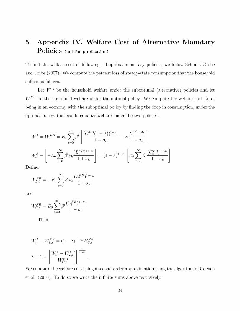
5 Appendix IV. Welfare Cost of Alternative Monetary

Policies (not for publication)

To find the welfare cost of following suboptimal monetary policies, we follow Schmitt-Grohe

and Uribe (2007). We compute the percent loss of steady-state consumption that the household

suffers as follows.

Let WA be the household welfare under the suboptimal (alternative) policies and let

W FB be the household welfare under the optimal policy. We compute the welfare cost, λ, of

being in an economy with the suboptimal policy by finding the drop in consumption, under the

optimal policy, that would equalize welfare under the two policies.

WAt = W FB

t = E0

∞∑t=0

βt

[(CFB

t (1− λ))1−σc

1− σc− νh

LFB1+σht

1 + σh

]

WAt −

[−E0

∞∑t=0

βtνh(LFBt )1+σh

1 + σh

]= (1− λ)1−σc

[E0

∞∑t=0

βt(CFB

t )1−σc

1− σc

]Define:

W FBL,t = −E0

∞∑t=0

βtνh(LFBt )1+σh

1 + σh

and

W FBC,t = E0

∞∑t=0

βt(CFB

t )1−σc

1− σc

Then

WAt −W FB

L,t = (1− λ)1−σcW FBC,t

λ = 1−

[WAt −W FB

L,t

W FBC,t

] 11−σc

.

We compute the welfare cost using a second-order approximation using the algorithm of Coenen

et al. (2010). To do so we write the infinite sums above recursively.

34

References

[1] Adao, Bernardino, Isabel Correia, and Pedro Teles, (2003), “Gaps and Triangles,” Review

of Economic Studies 70, pp. 699-713.

[2] Angelini, Paolo, Stefano Neri and Fabio Panetta, (2014), “The Interaction Between Capital

Requirements and Monetary Policy,” Journal of Money, Credit, and Banking 46(6), pp.

1073-1112.

[3] Angeloni, Ignazio and Ester Faia, (2013), “Capital Regulation and Monetary Policy with

Fragile Banks,” Journal of Monetary Economics 60, pp. 311-324.

[4] Beau, Denis, Clerc, Laurent, and Benoıt Mojon, (2011), “Macro-Prudential Policy and the

Conduct of Monetary Policy,” Banque de France Working Papers.

[5] Benigno, Pierpaolo and Michael Woodford (2005), “Inflation Stabilization and Welfare:

The Case of a Distorted Steady State,” Journal of the European Economic Association

3, pp. 1185-1236.

[6] Bernanke, Ben, and Mark Gertler (1999), “Monetary Policy and Asset Volatility,” Federal

Reserve Bank of Kansas City Economic Review, Fourth Quarter 1999, 84(4), pp. 17-52.

[7] Bernanke, Ben and Mark Gertler (2001), “Should Central Banks Respond to Movements

in Asset Prices,” American Economic Review Papers and Proceedings 91, 253-257.

[8] Bernanke, Ben, Mark Gertler, and Simon Gilchrist (1999), The Financial Accelerator in

a Quantitative Business Cycle Framework,” in John B. Taylor and Michael Woodford,

eds., Handbook of Macroeconomics, vol. 1C, Amsterdam: North-Holland.

[9] Brunnermeier, Markus K. and Yuliy Sannikov (2011), “A Macroeconomic Model with a

Financial Sector,” manuscript.

[10] Carlstrom, Charles C. and Timothy S. Fuerst (1997), “Agency Costs, Net Worth, and Busi-

ness Fluctuations: A Computable General Equilibrium Analysis,” American Economic

Review 87, pp.893-910.

35

[11] Carlstom, Charles T. C., Timothy S. Fuerst, and Matthias Paustian (2010), “Optimal

Monetary Policy In a Model with Agency Costs,” Journal of Money Credit and Banking,

42(1), pp. 37-70.

[12] Collard, Fabrice, Dellas, Harris, Diba, Behzad, and Olivier Loisel (2013), “Optimal Mon-

etary and Prudential Policies,” manuscript.

Christensen, Ian, Cesaire Meh, and Kevin Moran, (2011), “Bank Leverage and Macroeco-

nomic Dynamics,” Bank of Canada Working Paper 2011-32.

[13] Christiano, Lawrence J., Roberto Motto, and Massimo Rostagno, (2003), “The Great

Depression and the Friedman-Schwartz Hypothesis,” Journal of Money, Credit and

Banking 35(6), pp. 1119-1198.

[14] Christiano, Lawrence J. and Daisuke Ikeda, (2011), “Government Policy, Credit markets

and the Economy,” NBER Working Paper 17142.

[15] Christiano, Lawrence J., Roberto Motto, and Massimo Rostagno, (2010), “Financial Fac-

tors in Economic Fluctuations,” ECB Working Paper 1192.

[16] Christiano, Lawrence J., Roberto Motto, and Massimo Rostagno, (2014), “Risk Shocks,”

American Economic Review 104(1), pp. 27-65.

[17] Claessens, Stijn, Ghosh, Swati R., and Roxana Mihet, (2014), “Macro-Prudential Policies

to Mitigate Financial System Vulnerabilities,” IMF Working paper 14/155.

[18] Coenen, Gunter, Lombardo, Giovanni, Smets, Frank and Roland Straub, (2010), “Interna-

tional Transmission and Monetary Policy Cooperation,” in Jordi Galı and Mark Gertler

(eds), International Dimensions of Monetary Policy, NBER, Cambridge, M.A., Chapter

3, 175-192.

[19] Collard, Fabrice, Dellas, Harris, Diba, Behzad, and Olivier Loisel, (2012), “Optimal Mon-

etary Policy and Prudential Policies,” Banque de France Document de Travail no. 413.

[20] Curdia, Vasco, and Michael Woodford, (2009) “Credit Frictions and Optimal Monetary

Policy,” BIS Working Paper #278, Bank for International Settlements.

36

[21] De Fiore, Fiorella, Pedro Teles and Oreste Tristani (2011), “Monetary Policy and the

Financiing of Firms,” American Economic Journals: Macroeconomics 3, pp. 1-31.

[22] De Fiore, Fiorella and Oreste Tristani (2013), “Optimal Monetary Policy in a Model of

the Credit Channel,” Economic Journal 123(571), pp. 906-931.

[23] Dennis, Richard (2004), “Solving for Optimal Simple Rules in Rational Expectations Mod-

els,”Journal of Economic Dynamics and Control 28(8), pp. 1635-1660.

[24] Faia, Ester and Tommaso Monacelli (2007), “Optimal Interest-Rate Rules, Asset Prices,

and Credit Frictions,” Journal of Economic Dynamics and Control 31, pp. 3228-3254.

[25] Federico, Pablo, Vegh, Carlos A. and Guillermo Vuletin, (2012), “Reserve Requirement

Policy Over the Business Cylce,” manuscript.

[26] Galı, Jordi, Gertler Mark, and David Lopez-Salido (2007), “Markups, Gaps, and the Wel-

fare Costs of Business Fluctuations,” Review of Economics and Statistics 89(1), pp.

44-59.

[27] Gertler, Mark and Peter Karadi, (2009), “A Model of Unconventional Monetary Policy,”

manuscript.

[28] Gertler, Mark and Nobuhiro Kiyotaki (2010), “Financial Intermediation and Credit Policy

in Business Cycle Analysis,” in Benjamin M. Friedman and Michael Woodford, eds,

Handbook of Monetary Economics, vol 3A, pp 547-600.

[29] Gilchrist, Simon and John V. Leahy (2002), “Monetary Policy and Asset Prices,” Journal

of Monetary Economics 49(1), pp. 75-97.

[30] Gilchrist, Simon and Masashi Saito (2008),“Expectations, Asset Prices, and Monetary

Policy: The Role of Learning,” in John Y. Campbell, ed. Asset Prices and Monetary

Policy, Chicago: University of Chicago Press.

[31] Gilchrist, Simon and Egon Zakrajsek, (2012), “Credit Supply Shocks and Economic Activ-

ity in a Financial Accelerator Model,” in Alan Blinder, Andrew Lo and Robert Solow

(eds), Rethinking the Financial Crisis.

37

[32] Kashyap, Anil and jeremy C. Stein, (2012), “The optimal Conduct of Monetary Policy with

Interest on Reserves, American Economic Journal: Macroeconomics 4, pp. 266-282.

[33] Kiyotaki, Nobuhiro and John H. Moore, (1997), “Credit Cycles,” Journal of Political

Economy, 105(2), pp. 211-248.

[34] Leduc, Sylvain and Jean-Marc Natal, (2011), “Should Central Banks Lean Against Asset

Prices,” Federal Reserve Bank of San Francisco Working Paper 2011-15.

[35] Natal, Jean-Marc, (2012), “Monetary Response to Oil Price Shocks,” Journal of Money,

Credit, and Banking 44, pp. 53-101.

[36] Quint, Dominic and Pau Rabanal, (2013), “Monetary and Macroprudential Policy in an

Estimated DSGE Model of the Euro Area,” IMF Working Paper 13/2009.

[37] Schmitt-Grohe, Stephanie and Martin Uribe, (2007), “Optimal, Simple, and Imple-

mentable Monetary and Fiscal Rules,” Journal of Monetary Economics 54, pp. 1702-

1725.

[38] Stein, Jeremy C. (2013), “Overheating in Credit Markets: Origins, Measurement, and

Policy Responses,”speech delivered at “Restoring Household Financial Stability after

the Great Recession: Why Household Balance Sheets Matter,”a symposium sponsored

by the Federal Reserve Bank of St. Louis.

[39] Stein, Jeremy C. (2014), “Incorporating Financial Stability Considerations Into a Monetary

Policy Framework,”speech delivered at the“International Research Forum on Monetary

Policy”organized by the European Central Bank, the Federal Reserve Board, the Cen-

ter for Financial Studies at the Goethe University, and the Georgetown Center for

Economic Research at Georgetown University.

[40] Taylor, Alan M., and Moritz Schularick, (2012). “Credit Booms Gone Bust: Monetary

Policy, Leverage Cycle, and Financial Crises 1870-2009,” American Economic Re-

view.102(2), pp. 1029-61.

[41] Tetlow, Robert J. (2006), “Monetary Policy, Asset Prices and Misspecification: The Robust

38

Approach to Bubbles with Model Uncertainty,” in Issues in Inflation Targeting (Ottawa:

The Bank of Canada).

[42] Walsh, Carl E. (2003), “Speed Limit Policies: The Output Gap and Optimal Monetary

Policy,” American Economic Review 93(1), pp. 265-278.

[43] Woodford, Michael (2003). Interest and Prices: Foundations of a Theory of Monetary

Policy, Princeton: Princeton University Press.

[44] Woodford, Michael (2012). “Inflation Targeting and Financial Stability, ”Sveriges Riksbank

Economic Review, pp. 7-32.

[45] Yellen, Janet L. (2009), “A Minsky Meltdown: Lessons for Central Bankers,”speech to

the 18th Annual Hyman P. Minsky Conference on the State of the U.S. and World

Economies—“Meeting the Challenges of the Financial Crisis”organized by the Levy

Economics Institute of Bard College, New York, NY.

39

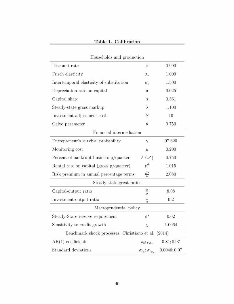
Table 1. Calibration

Households and production

Discount rate β 0.990

Frisch elasticity σh 1.000

Intertemporal elasticity of substitution σc 1.500

Depreciation rate on capital δ 0.025

Capital share α 0.361

Steady-state gross markup λ 1.100

Investment adjustment cost S 10

Calvo parameter θ 0.750

Financial intermediation

Entrepreneur’s survival probability γ 97.620

Monitoring cost µ 0.200

Percent of bankrupt business p/quarter F (ω?) 0.750

Rental rate on capital (gross p/quarter) Rk 1.015

Risk premium in annual percentage terms Rk

R2.080

Steady-state great ratios

Capital-output ratio ky

8.08

Investment-output ratio iy

0.2

Macroprudential policy

Steady-State reserve requirement φ∗ 0.02

Sensitivity to credit growth χ 1.0064

Benchmark shock processes: Christiano et al. (2014)

AR(1) coefficients ρa; ρσω 0.81; 0.97

Standard deviations σεa ;σεσω 0.0046; 0.07

40

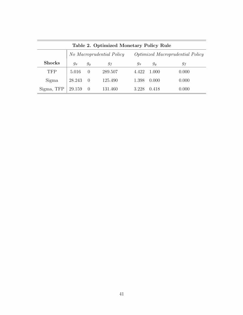
Table 2. Optimized Monetary Policy Rule

No Macroprudential Policy Optimized Macroprudential Policy

Shocks gπ gy gf gπ gy gf

TFP 5.016 0 289.507 4.422 1.000 0.000

Sigma 28.243 0 125.490 1.398 0.000 0.000

Sigma, TFP 29.159 0 131.460 3.228 0.418 0.000

41

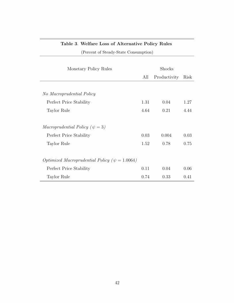
Table 3. Welfare Loss of Alternative Policy Rules

(Percent of Steady-State Consumption)

Monetary Policy Rules Shocks

All Productivity Risk

No Macroprudential Policy

Perfect Price Stability 1.31 0.04 1.27

Taylor Rule 4.64 0.21 4.44

Macroprudential Policy (ψ = 3)

Perfect Price Stability 0.03 0.004 0.03

Taylor Rule 1.52 0.78 0.75

Optimized Macroprudential Policy (ψ = 1.0064)

Perfect Price Stability 0.11 0.04 0.06

Taylor Rule 0.74 0.33 0.41

42

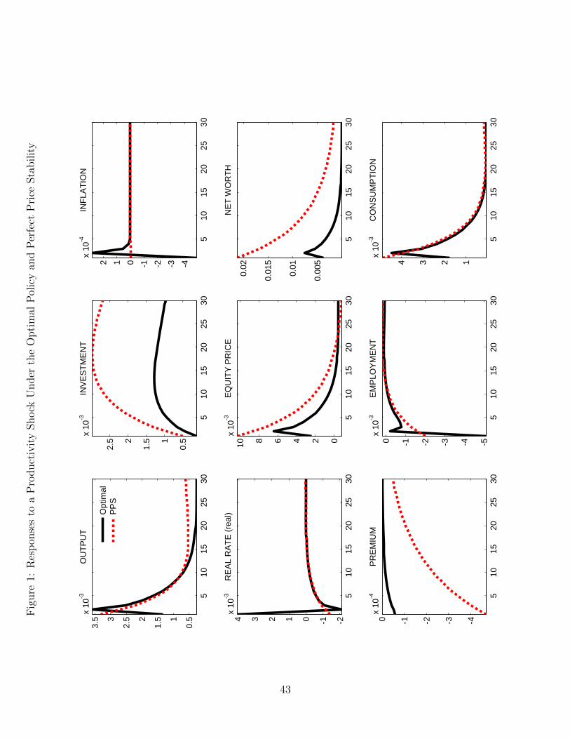
Fig

ure

1:R

esp

onse

sto

aP

roduct

ivit

yShock

Under

the

Opti

mal

Pol

icy

and

Per

fect

Pri

ceSta

bilit

y

510

1520

2530

0.51

1.52

2.53

3.5

x 10

-3O

UTP

UT

510

1520

2530

0.51

1.52

2.5

x 10

-3IN

VE

STM

EN

T

510

1520

2530

-4-3-2-1012

x 10

-4IN

FLA

TIO

N

510

1520

2530

-2-101234x

10-3

RE

AL

RA

TE (r

eal)

510

1520

2530

0246810x

10-3

EQ

UIT

Y P

RIC

E

510

1520

2530

0.00

5

0.01

0.01

5

0.02

NE

T W

OR

TH

510

1520

2530

-4-3-2-10x

10-4

PR

EM

IUM

510

1520

2530

-5-4-3-2-10x

10-3

EM

PLO

YM

EN

T

510

1520

2530

1234

x 10

-3C

ON

SU

MP

TIO

N

Opt

imal

PP

S

43

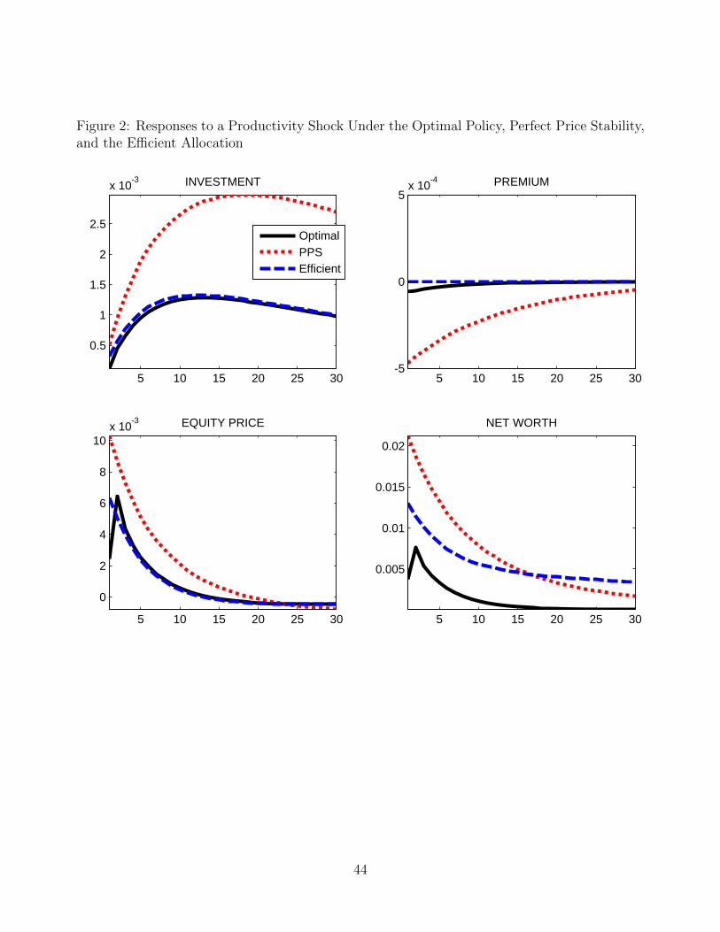
Figure 2: Responses to a Productivity Shock Under the Optimal Policy, Perfect Price Stability,and the Efficient Allocation

5 10 15 20 25 30

0.5

1

1.5

2

2.5

x 10-3 INVESTMENT

5 10 15 20 25 30-5

0

5x 10-4 PREMIUM

5 10 15 20 25 30

0

2

4

6

8

10x 10-3 EQUITY PRICE

5 10 15 20 25 30

0.005

0.01

0.015

0.02

NET WORTH

OptimalPPSEfficient

44

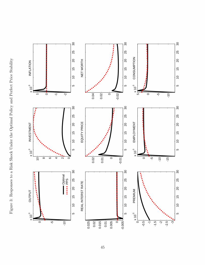
Fig

ure

3:R

esp

onse

sto

aR

isk

Shock

Under

the

Opti

mal

Pol

icy

and

Per

fect

Pri

ceSta

bilit

y

510

1520

2530

-10-50

x 10

-3O

UTP

UT

Opt

imal

PP

S

510

1520

2530

0246810

x 10

-3IN

VE

STM

EN

T

510

1520

2530

-2-101

x 10

-3IN

FLA

TIO

N

510

1520

2530

-0.0

050

0.00

5

0.01

0.01

5

0.02

0.02

5

RE

AL

INTE

RS

T R

ATE

510

1520

2530

-0.0

10

0.01

0.02

EQ

UIT

Y P

RIC

E

510

1520

2530

-0.0

20

0.02

0.04

NE

T W

OR

TH

510

1520

2530

-3

-2.5-2

-1.5-1

-0.50

x 10

-3P

RE

MIU

M

510

1520

2530

-15

-10-50

x 10

-3E

MP

LOY

ME

NT

510

1520

2530

-10-505

x 10

-3C

ON

SU

MP

TIO

N

45

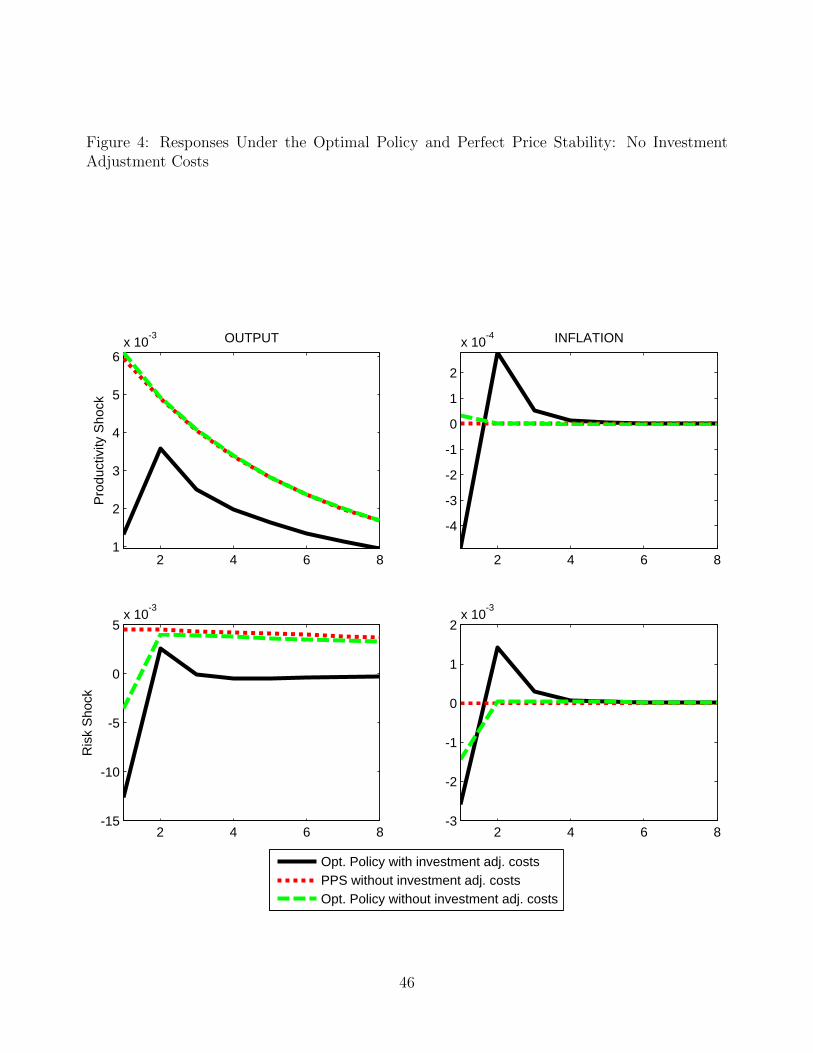
Figure 4: Responses Under the Optimal Policy and Perfect Price Stability: No InvestmentAdjustment Costs

2 4 6 81

2

3

4

5

6x 10-3 OUTPUT

Pro

duct

ivity

Sho

ck

2 4 6 8

-4

-3

-2

-1

0

1

2

x 10-4 INFLATION

2 4 6 8-15

-10

-5

0

5x 10-3

Ris

k S

hock

2 4 6 8-3

-2

-1

0

1

2x 10-3

Opt. Policy with investment adj. costsPPS without investment adj. costsOpt. Policy without investment adj. costs

46

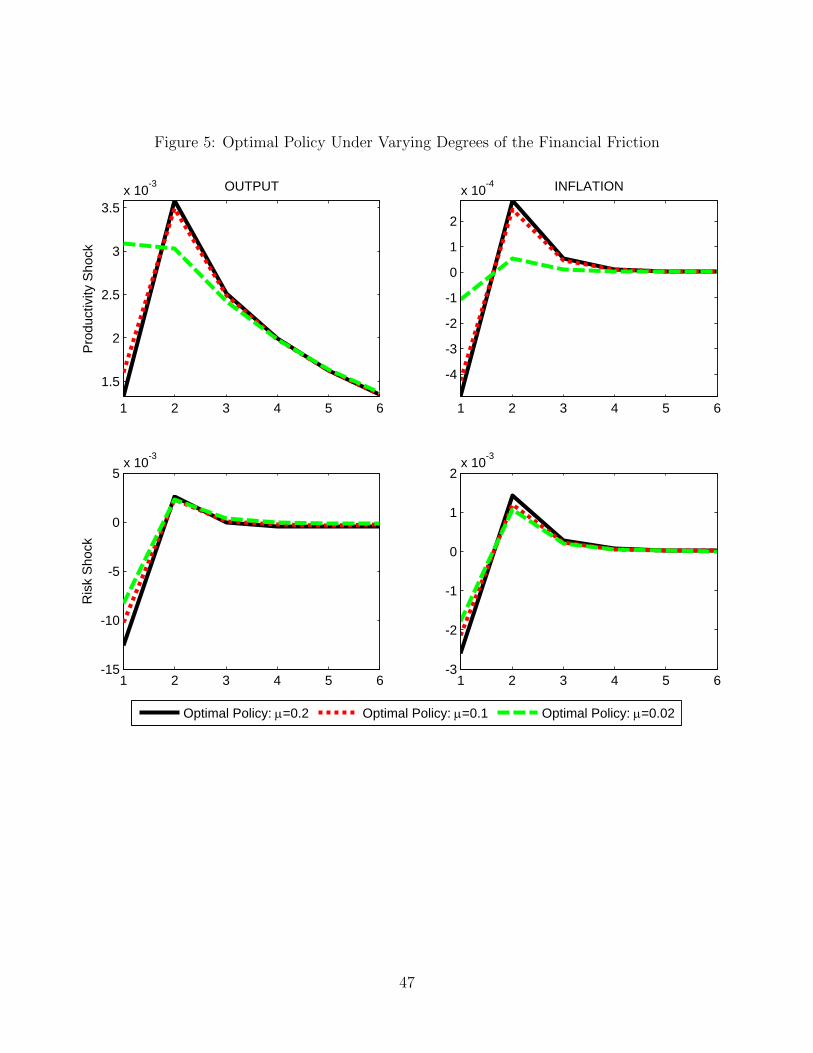
Figure 5: Optimal Policy Under Varying Degrees of the Financial Friction

1 2 3 4 5 6

1.5

2

2.5

3

3.5x 10-3 OUTPUT

Pro

duct

ivity

Sho

ck

1 2 3 4 5 6

-4

-3

-2

-1

0

1

2

x 10-4 INFLATION

1 2 3 4 5 6-15

-10

-5

0

5x 10-3

Ris

k S

hock

1 2 3 4 5 6-3

-2

-1

0

1

2x 10-3

Optimal Policy: =0.2 Optimal Policy: =0.1 Optimal Policy: =0.02

47

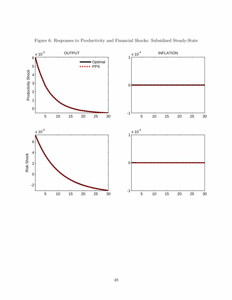
Figure 6: Responses to Productivity and Financial Shocks: Subsidized Steady-State

5 10 15 20 25 30

0

1

2

3

4

5

6x 10-3

Pro

duct

ivity

Sho

ck

OUTPUT

OptimalPPS

5 10 15 20 25 30-1

0

1x 10-4 INFLATION

5 10 15 20 25 30

-2

0

2

4

6

x 10-3

Ris

k S

hock

5 10 15 20 25 30-1

0

1x 10-4

48

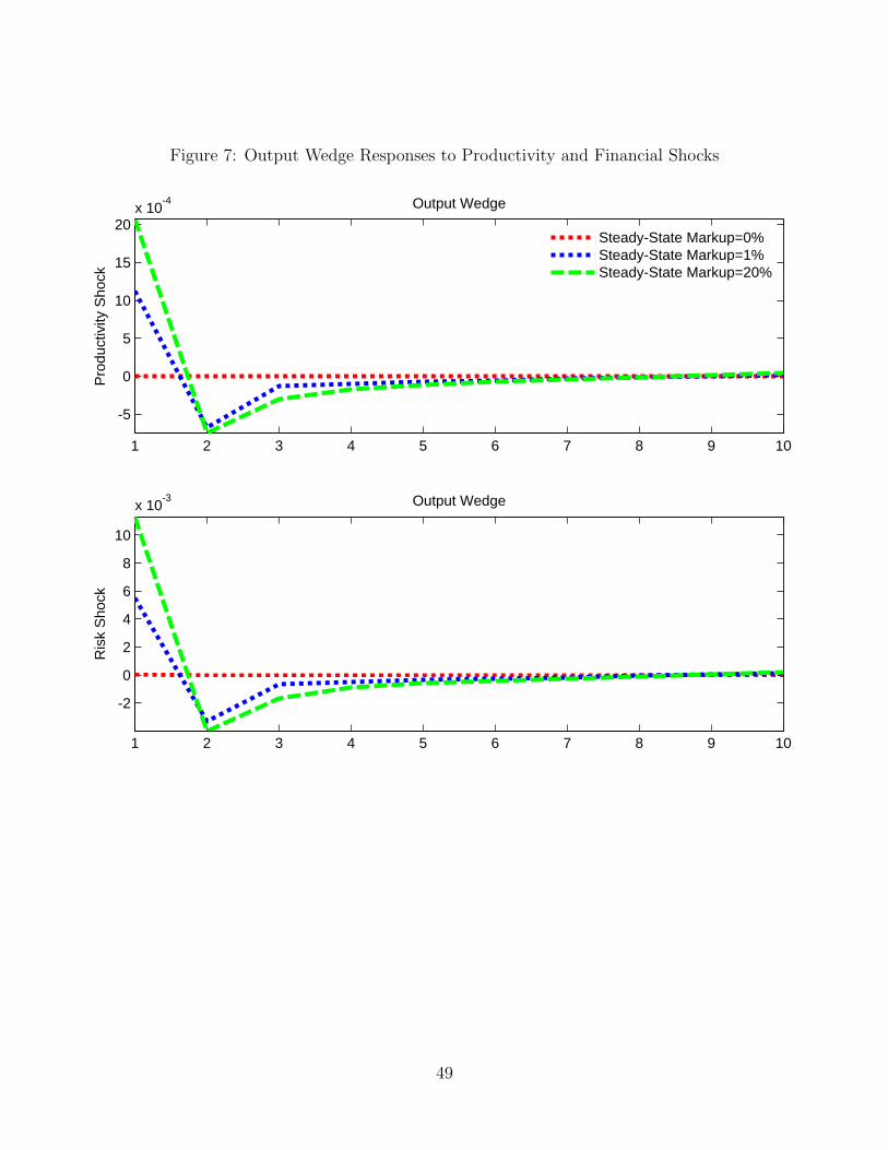
Figure 7: Output Wedge Responses to Productivity and Financial Shocks

1 2 3 4 5 6 7 8 9 10

-5

0

5

10

15

20x 10-4 Output Wedge

Pro

duct

ivity

Sho

ck

Steady-State Markup=0%Steady-State Markup=1%Steady-State Markup=20%

1 2 3 4 5 6 7 8 9 10

-2

0

2

4

6

8

10

x 10-3 Output Wedge

Ris

k S

hock

49

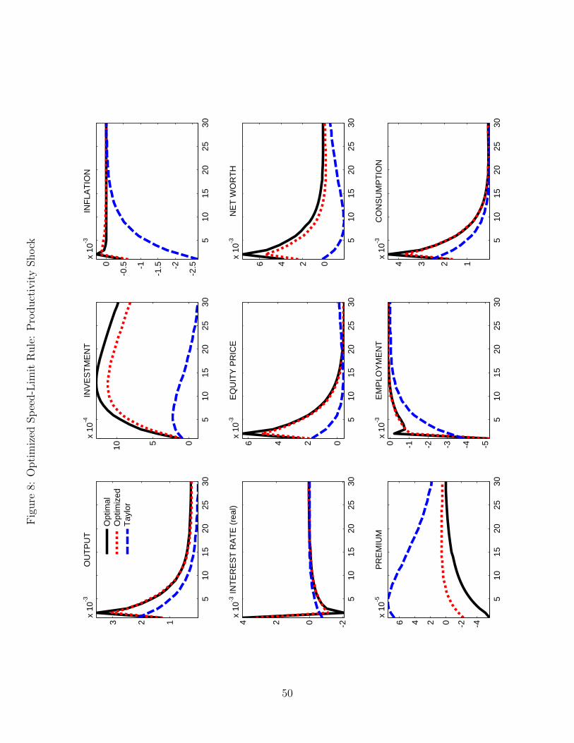
Fig

ure

8:O

pti

miz

edSp

eed-L

imit

Rule

:P

roduct

ivit

yShock

510

1520

2530

123

x 10

-3O

UTP

UT

O

ptim

alO

ptim

ized

Tayl

or

510

1520

2530

0510

x 10

-4IN

VE

STM

EN

T

510

1520

2530

-2.5-2

-1.5-1

-0.50

x 10

-3IN

FLA

TIO

N

510

1520

2530

-2024x

10-3

INTE

RE

ST

RA

TE (r

eal)

510

1520

2530

0246x

10-3

EQ

UIT

Y P

RIC

E

510

1520

2530

0246

x 10

-3N

ET

WO

RTH

510

1520

2530

-4-20246

x 10

-5P

RE

MIU

M

510

1520

2530

-5-4-3-2-10x

10-3

EM

PLO

YM

EN

T

510

1520

2530

1234

x 10

-3C

ON

SU

MP

TIO

N

50

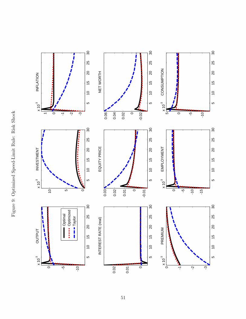
Fig

ure

9:O

pti

miz

edSp

eed-L

imit

Rule

:R

isk

Shock

510

1520

2530

-10-50

x 10

-3O

UTP

UT

Opt

imal

Opt

imiz

edTa

ylor

510

1520

2530

0510

x 10

-3IN

VE

STM

EN

T

510

1520

2530

-3-2-101

x 10

-3IN

FLA

TIO

N

510

1520

2530

0

0.01

0.02

INTE

RE

ST

RA

TE (r

eal)

510

1520

2530

-0.0

10

0.01

0.02

0.03

EQ

UIT

Y P

RIC

E

510

1520

2530

-0.0

20

0.02

0.04

0.06

NE

T W

OR

TH

510

1520

2530

-3-2-10x

10-3

PR

EM

IUM

510

1520

2530

-15

-10-50

x 10

-3E

MP

LOY

ME

NT

510

1520

2530

-10-505

x 10

-3C

ON

SU

MP

TIO

N

51

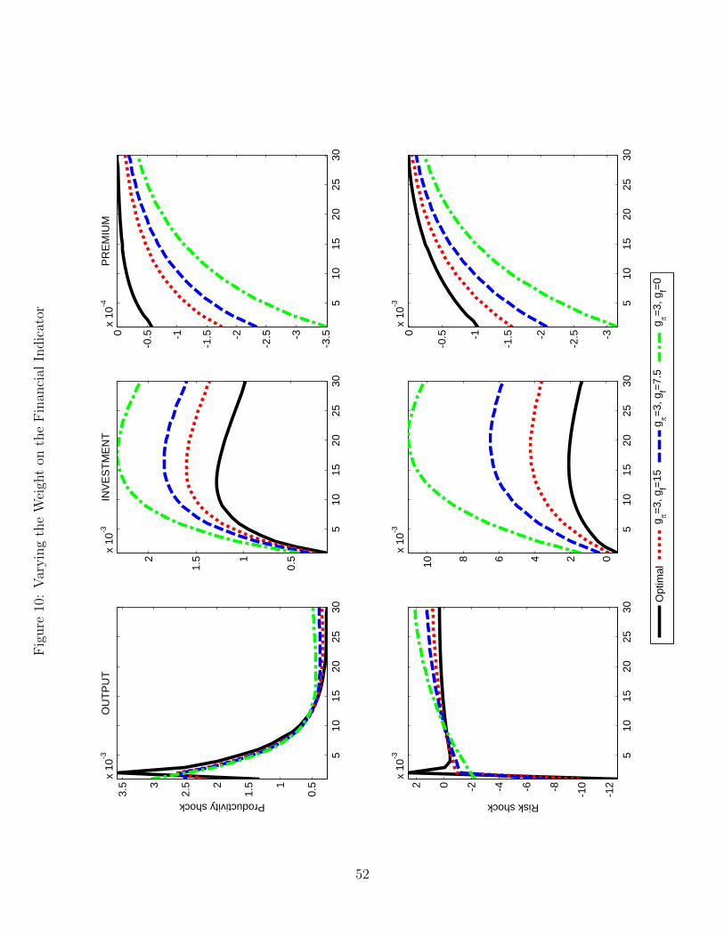
Fig

ure

10:

Var

yin

gth

eW

eigh

ton

the

Fin

anci

alIn

dic

ator

510

1520

2530

0.51

1.52

2.53

3.5

x 10

-3O

UTP

UT

Productivity shock

510

1520

2530

0.51

1.52

x 10

-3IN

VE

STM

EN

T

510

1520

2530

-3.5-3

-2.5-2

-1.5-1

-0.50

x 10

-4P

RE

MIU

M

510

1520

2530

-12

-10-8-6-4-202

x 10

-3

Risk shock

510

1520

2530

0246810

x 10

-3

510

1520

2530

-3

-2.5-2

-1.5-1

-0.50

x 10

-3

Opt

imal

g =3

, gf=1

5g

=3, g

f=7.5

g =3

, gf=0

52

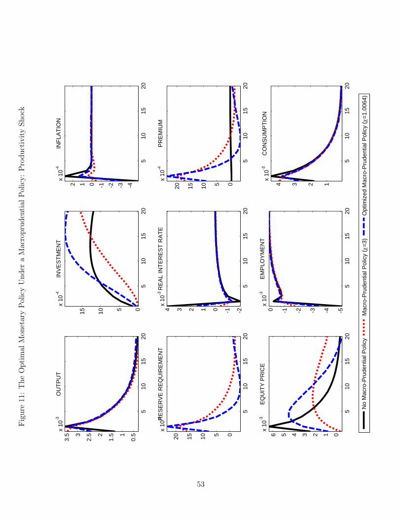
Fig

ure

11:

The

Opti

mal

Mon

etar

yP

olic

yU

nder

aM

acro

pru

den

tial

Pol

icy:

Pro

duct

ivit

yShock

510

1520

0.51

1.52

2.53

3.5

x 10

-3O

UTP

UT

510

1520

051015

x 10

-4IN

VE

STM

EN

T

510

1520

-4-3-2-1012

x 10

-4IN

FLA

TIO

N

510

1520

05101520

x 10

-4 RE

SE

RV

E R

EQ

UIR

EM

EN

T

510

1520

-2-101234x

10-3

RE

AL

INTE

RE

ST

RA

TE

510

1520

05101520

x 10

-4P

RE

MIU

M

510

1520

0123456x

10-3

EQ

UIT

Y P

RIC

E

510

1520

-5-4-3-2-10x

10-3

EM

PLO

YM

EN

T

510

1520

1234

x 10

-3C

ON

SU

MP

TIO

N

No

Mac

ro-P

rude

ntia

l Pol

icy

Mac

ro-P

rude

ntia

l Pol

icy

(=3

)O

ptim

ized

Mac

ro-P

rude

ntia

l Pol

icy

(=1

.006

4)

53

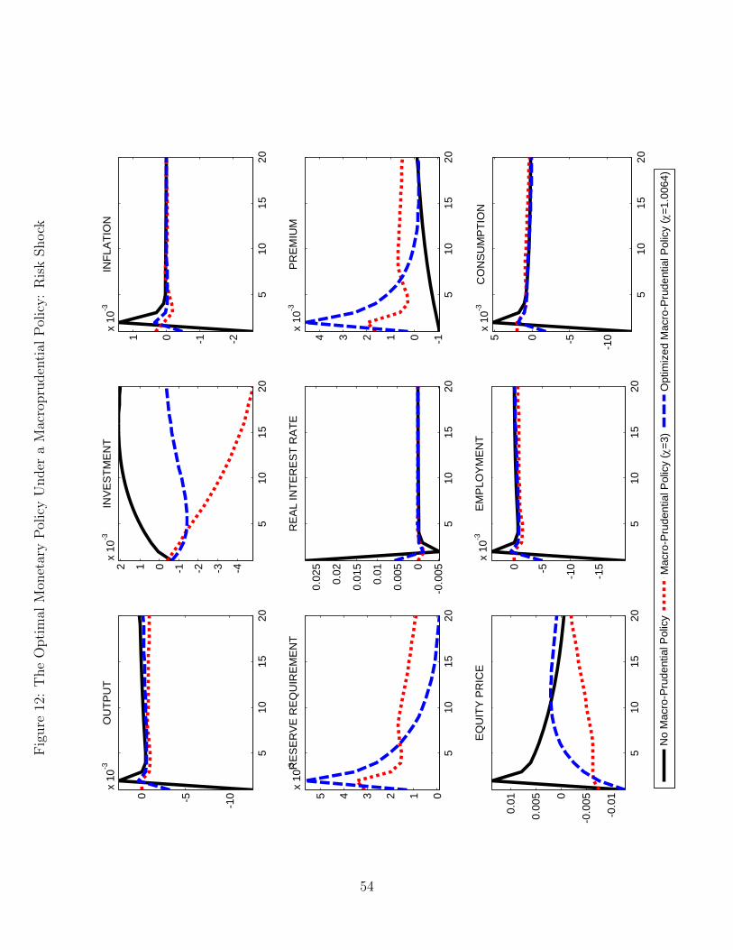
Fig

ure

12:

The

Opti

mal

Mon

etar

yP

olic

yU

nder

aM

acro

pru

den

tial

Pol

icy:

Ris

kShock

510

1520

-10-50

x 10

-3O

UTP

UT

510

1520

-4-3-2-1012x

10-3

INV

ES

TME

NT

510

1520

-2-101

x 10

-3IN

FLA

TIO

N

510

1520

012345

x 10

-3 RE

SE

RV

E R

EQ

UIR

EM

EN

T

510

1520

-0.0

050

0.00

5

0.01

0.01

5

0.02

0.02

5

RE

AL

INTE

RE

ST

RA

TE

510

1520

-101234

x 10

-3P

RE

MIU

M

510

1520

-0.0

1

-0.0

050

0.00

5

0.01

EQ

UIT

Y P

RIC

E

510

1520

-15

-10-50

x 10

-3E

MP

LOY

ME

NT

510

1520

-10-505

x 10

-3C

ON

SU

MP

TIO

N

No

Mac

ro-P

rude

ntia

l Pol

icy

Mac

ro-P

rude

ntia

l Pol

icy

(=3

)O

ptim

ized

Mac

ro-P

rude

ntia

l Pol

icy

(=1

.006

4)

54