Short-Text Semantic Similarity: Algorithms and

Applications

by

Md Arafat Sultan

B.Sc. Computer Science, University of Dhaka, 2007

M.S. Computer Science, University of Dhaka, 2009

M.S. Computer Science, University of Colorado Boulder, 2013

A thesis submitted to the

Faculty of the Graduate School of the

University of Colorado in partial fulfillment

of the requirements for the degree of

Doctor of Philosophy

Department of Computer Science

2016

This thesis entitled:Short-Text Semantic Similarity: Algorithms and Applications

written by Md Arafat Sultanhas been approved for the Department of Computer Science

Tamara Sumner

James Martin

Martha Palmer

Date

The final copy of this thesis has been examined by the signatories, and we find that both thecontent and the form meet acceptable presentation standards of scholarly work in the above

mentioned discipline.

Sultan, Md Arafat (Ph.D., Computer Science)

Short-Text Semantic Similarity: Algorithms and Applications

Thesis directed by Prof. Tamara Sumner

Short snippets of written text play a central role in our day-to-day communication—sms

and email messages, news headlines, tweets, and image captions are some of the many forms

in which we see them used every day. Natural language processing (nlp) techniques have

provided means for automatically processing such textual data at scale, supporting key

applications in areas like education, law, healthcare, and security. This dissertation explores

automatic identification of semantic similarity for short text: given two snippets, neither

longer than a few sentences, the goal is to develop algorithms that can quantify the degree of

their semantic similarity.

Short text similarity (sts) is an important problem in contemporary nlp, with ap-

plications in numerous real-life tasks. In academic tests, for example, student responses to

short-answer questions can be automatically graded based on their semantic similarity with

expert-provided correct answers to those questions. Automatic question answering (qa) is

another example, where textual similarity with the question is used to evaluate candidate

answer snippets retrieved from larger documents.

Semantic analysis of short text, however, is a challenging task—complex human expres-

sions can be encoded in just a few words, and sentences that look quite different on the surface

can express very similar meanings. This research contributes to the automatic identification

of short text similarity (sts) through the development and application of algorithms that

can align semantically similar concepts in the two snippets. The proposed sts algorithms are

applied to the real-life tasks of short answer grading and question answering. All algorithms

demonstrate state-of-the-art results in the respective tasks.

In view of the high utility of sts, statistical domain adaptation techniques are also

iv

explored for the proposed sts algorithms. Given training examples from different domains,

these techniques enable (1) joint learning of per-domain parameters (i.e. a separate set of

model parameters for each domain), and (2) inductive transfer among the domains for a

supervised sts model. Across text from different sources and applications, domain adaptation

improves overall performance of the proposed sts models.

Dedication

To my parents.

vi

Acknowledgements

This work would not have been possible without the advice and support of some

remarkable people. I don’t know how to thank Tammy enough; she is the best advisor

one could have, and has been an endless source of support and inspiration for me. I thank

Jim and Martha for being such great mentors; I will always be inspired by their knowledge

and personality. Working with Steve during my early years gave me the self-confidence I

needed to do independent research; thank you very much Steve! I thank Jordan for his

help and guidance; I learned key research skills working with him. A big thanks goes to my

labmates and collaborators: Ovo, David, Keith, Soheil, Ifeyinwa, Srinjita, Heather, Holly,

Katie, Daniela, and Bill. Finally, the person whose infinite patience and persistence made it

possible for me to stay focused on my work is my beautiful wife Salima. Thanks Salima, I

cannot imagine traveling down this path without you.

Contents

Chapter

1 Introduction 1

1.1 Short-Text Semantic Similarity (sts) . . . . . . . . . . . . . . . . . . . . . . 2

1.2 The Utility of sts . . . . . . . . . . . . . . . . . . . . . . . . . . . . . . . . . 3

1.3 Research Questions and Studies . . . . . . . . . . . . . . . . . . . . . . . . . 4

1.4 Contributions . . . . . . . . . . . . . . . . . . . . . . . . . . . . . . . . . . . 9

2 Monolingual Alignment: Identifying Related Concepts in Short Text Pairs 10

2.1 The Alignment Problem . . . . . . . . . . . . . . . . . . . . . . . . . . . . . 11

2.2 Alignment: Key Pieces of the Puzzle . . . . . . . . . . . . . . . . . . . . . . 12

2.3 Unsupervised Alignment Using Lexical and Contextual Similarity . . . . . . 14

2.3.1 System Description . . . . . . . . . . . . . . . . . . . . . . . . . . . . 15

2.3.2 Evaluation . . . . . . . . . . . . . . . . . . . . . . . . . . . . . . . . . 26

2.3.3 Discussion . . . . . . . . . . . . . . . . . . . . . . . . . . . . . . . . . 32

2.4 Two-Stage Logistic Regression for Supervised Alignment . . . . . . . . . . . 34

2.4.1 System Description . . . . . . . . . . . . . . . . . . . . . . . . . . . . 34

2.4.2 Features . . . . . . . . . . . . . . . . . . . . . . . . . . . . . . . . . . 36

2.4.3 Experiments . . . . . . . . . . . . . . . . . . . . . . . . . . . . . . . . 40

2.4.4 Discussion . . . . . . . . . . . . . . . . . . . . . . . . . . . . . . . . . 45

2.5 Conclusions . . . . . . . . . . . . . . . . . . . . . . . . . . . . . . . . . . . . 46

viii

3 Algorithms for Short-Text Semantic Similarity 47

3.1 Short-Text Semantic Similarity . . . . . . . . . . . . . . . . . . . . . . . . . 47

3.2 Literature Review . . . . . . . . . . . . . . . . . . . . . . . . . . . . . . . . . 49

3.3 The SemEval Semantic Textual Similarity 2012–2015 Corpus . . . . . . . . . 52

3.4 Short Text Similarity from Alignment . . . . . . . . . . . . . . . . . . . . . . 53

3.4.1 System Description . . . . . . . . . . . . . . . . . . . . . . . . . . . . 54

3.4.2 Evaluation . . . . . . . . . . . . . . . . . . . . . . . . . . . . . . . . . 54

3.5 A Supervised sts Model . . . . . . . . . . . . . . . . . . . . . . . . . . . . . 58

3.5.1 System Description . . . . . . . . . . . . . . . . . . . . . . . . . . . . 59

3.5.2 Evaluation . . . . . . . . . . . . . . . . . . . . . . . . . . . . . . . . . 60

3.6 Conclusions and Future Work . . . . . . . . . . . . . . . . . . . . . . . . . . 64

4 Short Text Similarity for Automatic Question Answering 65

4.1 Background . . . . . . . . . . . . . . . . . . . . . . . . . . . . . . . . . . . . 67

4.1.1 Answer Sentence Ranking . . . . . . . . . . . . . . . . . . . . . . . . 67

4.1.2 Answer Extraction . . . . . . . . . . . . . . . . . . . . . . . . . . . . 68

4.1.3 Coupled Ranking and Extraction . . . . . . . . . . . . . . . . . . . . 70

4.2 Approach . . . . . . . . . . . . . . . . . . . . . . . . . . . . . . . . . . . . . 71

4.2.1 Answer Sentence Ranking . . . . . . . . . . . . . . . . . . . . . . . . 71

4.2.2 Answer Extraction . . . . . . . . . . . . . . . . . . . . . . . . . . . . 72

4.2.3 Joint Ranking and Extraction . . . . . . . . . . . . . . . . . . . . . . 72

4.2.4 Learning . . . . . . . . . . . . . . . . . . . . . . . . . . . . . . . . . . 74

4.3 Answer Sentence Ranking Features . . . . . . . . . . . . . . . . . . . . . . . 74

4.4 Answer Extraction Features . . . . . . . . . . . . . . . . . . . . . . . . . . . 75

4.4.1 Question-Independent Features . . . . . . . . . . . . . . . . . . . . . 76

4.4.2 Features Containing the Question Type . . . . . . . . . . . . . . . . . 76

4.5 Experiments . . . . . . . . . . . . . . . . . . . . . . . . . . . . . . . . . . . . 79

ix

4.5.1 Data . . . . . . . . . . . . . . . . . . . . . . . . . . . . . . . . . . . . 79

4.5.2 Answer Sentence Ranking . . . . . . . . . . . . . . . . . . . . . . . . 80

4.5.3 Answer Extraction . . . . . . . . . . . . . . . . . . . . . . . . . . . . 82

4.6 Discussion . . . . . . . . . . . . . . . . . . . . . . . . . . . . . . . . . . . . . 87

4.7 Conclusions and Future Work . . . . . . . . . . . . . . . . . . . . . . . . . . 87

5 Short Answer Grading using Text Similarity 89

5.1 sts and Short Answer Grading . . . . . . . . . . . . . . . . . . . . . . . . . 90

5.2 Related Work . . . . . . . . . . . . . . . . . . . . . . . . . . . . . . . . . . . 91

5.3 Method . . . . . . . . . . . . . . . . . . . . . . . . . . . . . . . . . . . . . . 92

5.3.1 Features . . . . . . . . . . . . . . . . . . . . . . . . . . . . . . . . . . 92

5.4 Experiments . . . . . . . . . . . . . . . . . . . . . . . . . . . . . . . . . . . . 94

5.4.1 The Mohler et al. [68] Task . . . . . . . . . . . . . . . . . . . . . . . 94

5.4.2 The SemEval-2013 Task . . . . . . . . . . . . . . . . . . . . . . . . . 96

5.4.3 Runtime Test . . . . . . . . . . . . . . . . . . . . . . . . . . . . . . . 97

5.4.4 Ablation Study . . . . . . . . . . . . . . . . . . . . . . . . . . . . . . 98

5.5 Conclusions . . . . . . . . . . . . . . . . . . . . . . . . . . . . . . . . . . . . 99

6 Domain Adaptation for Short Text Similarity 100

6.1 Tasks and Datasets . . . . . . . . . . . . . . . . . . . . . . . . . . . . . . . . 101

6.2 Bayesian Domain Adaptation for sts . . . . . . . . . . . . . . . . . . . . . . 103

6.2.1 Base Models . . . . . . . . . . . . . . . . . . . . . . . . . . . . . . . . 103

6.2.2 Adaptation to sts Domains . . . . . . . . . . . . . . . . . . . . . . . 105

6.2.3 Multitask Learning . . . . . . . . . . . . . . . . . . . . . . . . . . . . 106

6.3 Features . . . . . . . . . . . . . . . . . . . . . . . . . . . . . . . . . . . . . . 107

6.4 Experiments . . . . . . . . . . . . . . . . . . . . . . . . . . . . . . . . . . . . 108

6.4.1 Adaptation to sts Domains . . . . . . . . . . . . . . . . . . . . . . . 109

6.4.2 Multitask Learning . . . . . . . . . . . . . . . . . . . . . . . . . . . . 113

x

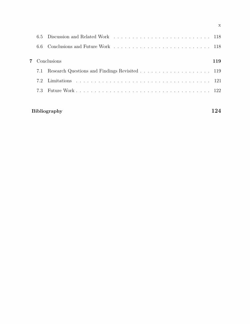
6.5 Discussion and Related Work . . . . . . . . . . . . . . . . . . . . . . . . . . 118

6.6 Conclusions and Future Work . . . . . . . . . . . . . . . . . . . . . . . . . . 118

7 Conclusions 119

7.1 Research Questions and Findings Revisited . . . . . . . . . . . . . . . . . . . 119

7.2 Limitations . . . . . . . . . . . . . . . . . . . . . . . . . . . . . . . . . . . . 121

7.3 Future Work . . . . . . . . . . . . . . . . . . . . . . . . . . . . . . . . . . . . 122

Bibliography 124

Tables

Table

1.1 Human-assigned similarity scores to sentence pairs [1]. . . . . . . . . . . . . 2

1.2 The relation between sts and question answering. Answer-bearing sentences

are likely to have semantically more in common with the question than sen-

tences not containing an answer. These examples are taken from the question

answering dataset reported in [104]. . . . . . . . . . . . . . . . . . . . . . . . 4

1.3 The relation between sts and short answer grading. The first student answer,

which covers the entire semantic content of the reference answer, received a

100% score from human graders. The second answer covers much less of the

reference answer’s content, receiving a score of only 40%. These examples are

taken from the dataset reported in [68]. . . . . . . . . . . . . . . . . . . . . . 5

2.1 Equivalent dependency structures. . . . . . . . . . . . . . . . . . . . . . . . . 19

2.2 Results of intrinsic evaluation on two datasets. . . . . . . . . . . . . . . . . . 27

2.3 Ablation test results. . . . . . . . . . . . . . . . . . . . . . . . . . . . . . . . 28

2.4 Performance on different word pair types. . . . . . . . . . . . . . . . . . . . . 30

2.5 Extrinsic evaluation on *SEM 2013 sts data. The sts system of Han et

al. [42] is the top-performing system at *SEM 2013; Yao et al. [108] report the

previous best monolingual aligner. . . . . . . . . . . . . . . . . . . . . . . . . 31

xii

2.6 Extrinsic evaluation on msr paraphrase data. Madnani et al. [42] have the

best performance on this dataset; Yao et al. [108, 109] report state-of-the-art

monolingual aligners. . . . . . . . . . . . . . . . . . . . . . . . . . . . . . . . 32

2.7 Performance on two alignment data sets. Improvements of the proposed

supervised aligners over other aligners in F1 are statistically significant. . . . 41

2.8 Extrinsic evaluation on *SEM 2013 sts data. . . . . . . . . . . . . . . . . . 42

2.9 Extrinsic evaluation on msr paraphrase data. . . . . . . . . . . . . . . . . . 42

2.10 Performance with and without stage 2. . . . . . . . . . . . . . . . . . . . . . 43

2.11 Results without different stage 1 features. . . . . . . . . . . . . . . . . . . . 44

2.12 Results without different stage 2 features. . . . . . . . . . . . . . . . . . . . 44

2.13 Performance on different word pair types. . . . . . . . . . . . . . . . . . . . . 45

3.1 Human-assigned similarity scores to pairs of sentences on a 0–5 scale. Examples

are taken from [1]. Interpretation of each similarity level is shown in Table 3.2. 48

3.2 Interpretations of the six similarity levels at SemEval Semantic Textual Simi-

larity [1]. . . . . . . . . . . . . . . . . . . . . . . . . . . . . . . . . . . . . . . 49

3.3 All datasets from SemEval sts 2012–2015. Average sentence lengths, measured

in number of words, are shown for all datasets. q&a: Questions and Answers;

mt: Machine Translation; iaa: Inter-Annotator Agreement. . . . . . . . . . 52

3.4 Performance of human annotators and different sts systems on SemEval STS

2012–2015 test sets. . . . . . . . . . . . . . . . . . . . . . . . . . . . . . . . . 56

3.5 Examples of sentence similarity scores computed by the unsupervised sts

algorithm. . . . . . . . . . . . . . . . . . . . . . . . . . . . . . . . . . . . . . 57

3.6 Different source domains of text at SemEval sts 2012–2015. . . . . . . . . . 60

3.7 Performance of human annotators and different sts systems on SemEval sts

2012–2015 test sets. . . . . . . . . . . . . . . . . . . . . . . . . . . . . . . . . 61

xiii

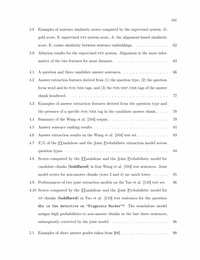
3.8 Examples of sentence similarity scores computed by the supervised system. G:

gold score, S: supervised sts system score, A: the alignment-based similarity

score, E: cosine similarity between sentence embeddings. . . . . . . . . . . . 62

3.9 Ablation results for the supervised sts system. Alignment is the more infor-

mative of the two features for most datasets. . . . . . . . . . . . . . . . . . 63

4.1 A question and three candidate answer sentences. . . . . . . . . . . . . . . . 66

4.2 Answer extraction features derived from (1) the question type, (2) the question

focus word and its pos/ner tags, and (3) the pos/dep/ner tags of the answer

chunk headword. . . . . . . . . . . . . . . . . . . . . . . . . . . . . . . . . . 77

4.3 Examples of answer extraction features derived from the question type and

the presence of a specific pos/ner tag in the candidate answer chunk. . . . . 78

4.4 Summary of the Wang et al. [104] corpus. . . . . . . . . . . . . . . . . . . . 79

4.5 Answer sentence ranking results. . . . . . . . . . . . . . . . . . . . . . . . . . 81

4.6 Answer extraction results on the Wang et al. [104] test set. . . . . . . . . . . 83

4.7 F1% of the STandalone and the Joint Probabilistic extraction model across

question types. . . . . . . . . . . . . . . . . . . . . . . . . . . . . . . . . . . 84

4.8 Scores computed by the STandalone and the Joint Probabilistic model for

candidate chunks (boldfaced) in four Wang et al. [104] test sentences. Joint

model scores for non-answer chunks (rows 2 and 4) are much lower. . . . . . 85

4.9 Performances of two joint extraction models on the Yao et al. [110] test set. 86

4.10 Scores computed by the STandalone and the Joint Probabilistic model for

np chunks (boldfaced) in Yao et al. [110] test sentences for the question:

Who is the detective on “Diagnosis Murder”? The standalone model

assigns high probabilities to non-answer chunks in the last three sentences,

subsequently corrected by the joint model. . . . . . . . . . . . . . . . . . . . 86

5.1 Examples of short answer grades taken from [68]. . . . . . . . . . . . . . . . 90

xiv

5.2 Performance on the Mohler et al. [68] dataset with out-of-domain training.

Performances of simpler bag-of-words models are reported by those authors. 95

5.3 Performance on the Mohler et al. [68] dataset with in-domain training. . . . 96

5.4 F1 scores on the SemEval-2013 datasets. . . . . . . . . . . . . . . . . . . . . 97

5.5 Ablation results on the Mohler et al. [68] dataset. . . . . . . . . . . . . . . 98

6.1 Ten different source domains at SemEval sts 2012–2015. . . . . . . . . . . . 102

6.2 The proposed Bayesian base models outperform the state of the art in sts,

sas and asr. . . . . . . . . . . . . . . . . . . . . . . . . . . . . . . . . . . . 108

6.3 Correlation ratios of the three models vs. the best model across sts domains.

Best scores are boldfaced, worst scores are underlined. The adaptive model

has the best (1) overall score, and (2) consistency across domains. . . . . . 111

6.4 Feature weights and correlations of different models in three extreme scenarios.

In each case, the adaptive model learns relative weights that are more similar

to those in the best baseline model. . . . . . . . . . . . . . . . . . . . . . . 112

6.5 Sentence pairs from smt and msrpar-test with gold similarity scores and

model errors (Global, Individual and Adaptive). The adaptive model error is

very close to the best model error in each case. . . . . . . . . . . . . . . . . 113

Figures

Figure

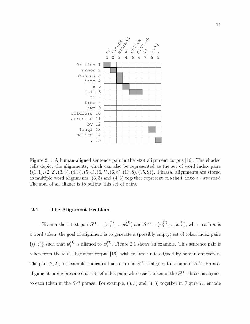
2.1 A human-aligned sentence pair in the msr alignment corpus [16]. The shaded

cells depict the alignments, which can also be represented as the set of word in-

dex pairs {(1, 1), (2, 2), (3, 3), (4, 3), (5, 4), (6, 5), (6, 6), (13, 8), (15, 9)}. Phrasal

alignments are stored as multiple word alignments: (3, 3) and (4, 3) together

represent crashed into ↔ stormed. The goal of an aligner is to output this

set of pairs. . . . . . . . . . . . . . . . . . . . . . . . . . . . . . . . . . . . . 11

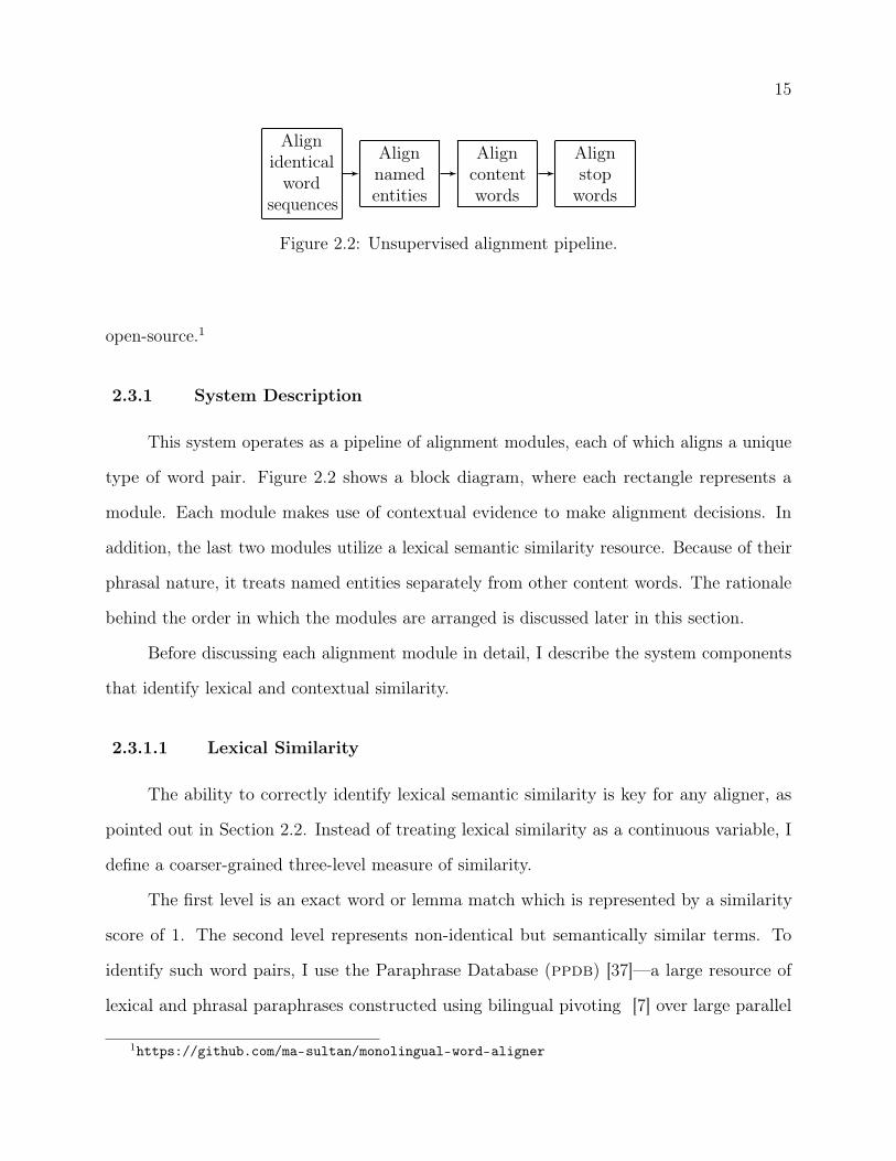
2.2 Unsupervised alignment pipeline. . . . . . . . . . . . . . . . . . . . . . . . . 15

2.3 Equivalent dependency types: dobj and rcmod . . . . . . . . . . . . . . . . . 17

2.4 Parent-child orientations in dependencies. . . . . . . . . . . . . . . . . . . . . 18

2.5 % distribution of aligned word pair types; nne: non-named entity, ne: named

entity, c: content word, f : function word, p: punctuation mark. . . . . . . . 29

2.6 Two-stage logistic regression for alignment. Stage 1 computes an alignment

probability φij for each word pair based on local features f (1)ij and learned

weights θ(1)tij (see Section 2.4.2.1). Stage 2 assigns each pair a label Aij ∈

{aligned, not aligned} based on its own φ, the φ of its cooperating and

competing pairs, a max-weighted bipartite matching Mφ with all φ values as

edge weights, the semantic similarities Sw of the pair’s words and words in all

cooperating pairs, and learned weights θ(2)tij for these global features. . . . . 35

xvi

2.7 Word and entity-based representations of a sentence. Words in the same named

entity are grouped together in the latter representation. . . . . . . . . . . . . 38

3.1 Alignment in semantically similar sentences. This sentence pair was judged

to be 80% similar by human annotators. There is also a very high degree of

semantic alignment between concepts (words and phrases) between the two

sentences. . . . . . . . . . . . . . . . . . . . . . . . . . . . . . . . . . . . . . 53

3.2 Alignment in semantically dissimilar sentences. This sentence pair was labeled

only 20% similar by human judges. The two sentences also have a very low

degree of semantic alignment. . . . . . . . . . . . . . . . . . . . . . . . . . . 54

6.1 Base models for sts, sas and asr. Plates represent replication across sentence

pairs. . . . . . . . . . . . . . . . . . . . . . . . . . . . . . . . . . . . . . . . . 104

6.2 Adaptation to different sts domains. The outer plate represents replication

across domains. Joint learning of a global weight vector w∗ along with

individual domain-specific vectors wd enables inductive transfer among domains.105

6.3 Multitask learning: sts, sas and asr. Global (w∗), task-specific (wsts, wsas,

wasr) and domain-specific (wd) weight vectors are jointly learned, enabling

transfer across domains and tasks. . . . . . . . . . . . . . . . . . . . . . . . . 106

6.4 A non-hierarchical joint model for sts, sas and asr. A common weight vector

w is learned for all tasks and domains. . . . . . . . . . . . . . . . . . . . . . 107

6.5 Results of adaptation to sts domains across different amounts of training data.

Table shows mean±SD from 20 random train/test splits. While the baselines

perform poorly at extremes, the adaptive model shows consistent performance. 110

6.6 Results of multitask learning for sts. Table shows mean±sd from 20 random

train/test splits. The adaptive model consistently performs well while the

baselines have different failure modes. . . . . . . . . . . . . . . . . . . . . . 114

xvii

6.7 Results of multitask learning for sas. Tables show mean±SD from 20 random

train/test splits. The adaptive model performs the best, and successfully

handles domain shift evident from the global model error. . . . . . . . . . . . 115

6.8 Results of multitask learning for asr. Tables show mean±SD from 20 random

train/test splits. Least affected by coarse-grained in-domain annotations, the

global model performs the best; the adaptive model stays close across all

training set sizes. . . . . . . . . . . . . . . . . . . . . . . . . . . . . . . . . . 116

Chapter 1

Introduction

Much of today’s human communication happens in the form of short snippets of written

text. News headlines, sms and emails, tweets, image captions—the use of short text is

extensive, spanning a variety of domains and applications. Analysis of such raw textual data

can reveal information that is important, even critical, in different areas of modern human

life: education, security, business, law, healthcare, and so forth. Unsurprisingly, processing of

short text—sentences for example—is a primary focus in classical and contemporary natural

language processing (nlp).

As a unit of analysis, however, short text presents unique challenges for nlp algorithms.

Unlike words, for example, an infinite number of meaningful sentences can be generated in

any human language. Each sentence is therefore too scarce as a unit to support effective

statistical analysis in its raw form. Unlike documents, on the other hand, sentences do not

generally have sufficient content for topical analysis to work properly. Within their brief

span, short text can accommodate the most complex and subtlest of human expressions,

necessitating semantic and syntactic analysis at a much deeper level than what is typically

required for words or documents. Fortunately, nlp has matured as a field to the point where

we have powerful algorithms for sentential semantics and syntax, which in turn has opened

up avenues for exciting new research.

This dissertation focuses on one such research problem: determination of semantic

similarity between two short snippets of text. On the one hand, short text similarity (sts)

2

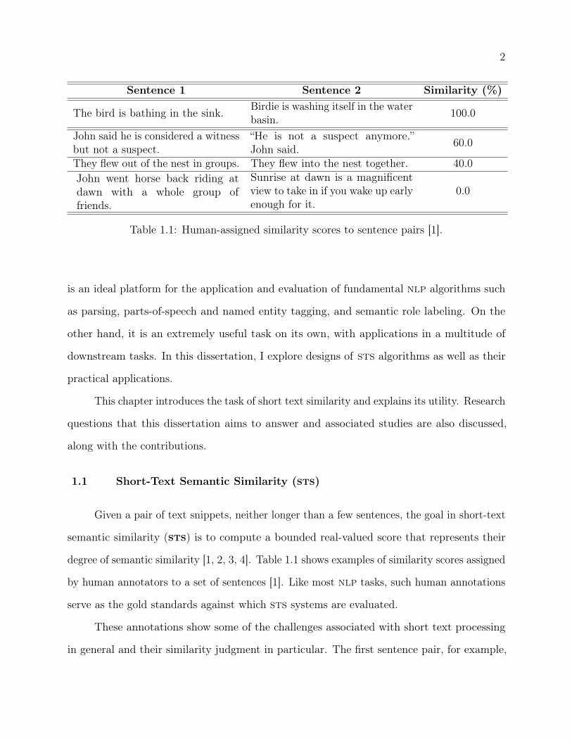
Sentence 1 Sentence 2 Similarity (%)

The bird is bathing in the sink. Birdie is washing itself in the waterbasin. 100.0

John said he is considered a witnessbut not a suspect.

“He is not a suspect anymore.”John said. 60.0

They flew out of the nest in groups. They flew into the nest together. 40.0John went horse back riding atdawn with a whole group offriends.

Sunrise at dawn is a magnificentview to take in if you wake up earlyenough for it.

0.0

Table 1.1: Human-assigned similarity scores to sentence pairs [1].

is an ideal platform for the application and evaluation of fundamental nlp algorithms such

as parsing, parts-of-speech and named entity tagging, and semantic role labeling. On the

other hand, it is an extremely useful task on its own, with applications in a multitude of

downstream tasks. In this dissertation, I explore designs of sts algorithms as well as their

practical applications.

This chapter introduces the task of short text similarity and explains its utility. Research

questions that this dissertation aims to answer and associated studies are also discussed,

along with the contributions.

1.1 Short-Text Semantic Similarity (sts)

Given a pair of text snippets, neither longer than a few sentences, the goal in short-text

semantic similarity (sts) is to compute a bounded real-valued score that represents their

degree of semantic similarity [1, 2, 3, 4]. Table 1.1 shows examples of similarity scores assigned

by human annotators to a set of sentences [1]. Like most nlp tasks, such human annotations

serve as the gold standards against which sts systems are evaluated.

These annotations show some of the challenges associated with short text processing

in general and their similarity judgment in particular. The first sentence pair, for example,

3

shows why unlike documents, exact term matching is inadequate for short text—the ability to

identify semantically similar words and phrases (e.g., sink and water basin) is an absolute

necessity. The pair with a 40% similarity shows how function words—words that are generally

considered to have little semantic value—can affect sentence meaning, and consequently,

human perception of similarity in text pairs with otherwise high term overlap.

sts poses numerous such challenges, a comprehensive treatment of all of which is

beyond the scope of a single dissertation. Instead, the aim of this dissertation is to capture

the fundamental requirements of sts in a simple set of actionable hypotheses and design

effective and efficient sts models that can be easily applied to real-life applications.

It is important to note the distinction between sts and the related tasks of paraphrase

detection and textual entailment recognition. In paraphrase detection [30, 61, 86], the goal is

to assign a binary label to a short text pair that indicates whether or not they are semantically

equivalent, as opposed to a real-valued score representing their degree of similarity. In textual

entailment recognition [23, 39], the output is again a binary variable, but one that indicates

whether the truth value of one snippet—the hypothesis—can be derived from that of the

other—the text. Unlike sts and paraphrase detection, entailment is thus directional: “S(1)

entails S(2)” does not necessarily mean “S(2) entails S(1).”

1.2 The Utility of sts

While sts can serve as an ideal testbed for fundamental nlp algorithms, its primary

utility lies in the large set of downstream tasks where it can be used as a system component.

Consider question answering (qa), for example. An important qa task is the identification

of answer-bearing sentences given a set of candidates. Table 1.2 shows a question Q and

two candidate answer sentences S(1) and S(2). Of the two candidates, only S(1) contains an

answer to Q. It is not entirely coincidental that it also has a greater semantic overlap with

Q than S(2)—answer-bearing sentences are generally expected to mention concepts about

which the question is being asked. While high semantic similarity with the question does not

4

Q What country is the biggest producer of tungsten?

S(1) China dominates world tungsten production and has frequently beenaccused of dumping tungsten on western markets.

S(2) Shanghai now has 26 foreign financial companies, the largest number inChina.

Table 1.2: The relation between sts and question answering. Answer-bearing sentences arelikely to have semantically more in common with the question than sentences not containingan answer. These examples are taken from the question answering dataset reported in [104].

guarantee the presence of an answer in a candidate sentence, it can definitely be useful in

filtering out bad candidates. Examples of answer sentence identification algorithms based on

semantic similarity can be found in [82, 104, 107].

Another real-life task that can benefit from sts is the grading of short answers in

academic tests. Given a correct reference answer to a short-answer question, student answers

can be evaluated based on their semantic similarity with the reference answer. Table 1.3

shows an example from a dataset of Data Structures questions in undergraduate Computer

Science [68]. The first student answer covers the entire semantic content of the reference

answer; as expected, human graders gave it a 100% score. The second answer, on the contrary,

received a much lower score of 40% as it covers much less of the reference answer’s content.

This dissertation closely examines the two above tasks as application areas for the

proposed sts models. Other applications of sts include evaluation of machine-translated text

[19, 58], redundancy identification during text summarization [25, 102], text reuse detection

[9, 21], and identification of core domain concepts in educational resources [90].

1.3 Research Questions and Studies

In view of sts as a high-utility task, this dissertation focuses on (1) the development of

fast, easy-to-replicate, and high-accuracy sts algorithms, and (2) their application to two

practical tasks: question answering and assessment of short student answers. Following are

5

Question: What is a stack?Reference Answer: A data structure that can store elements, which has the property thatthe last item added will be the first to be removed (or last-in-first-out).

Student Answer GradeA data structure for storing items which are to be accessed in last-in first-out order 100%that can be implemented in three ways.Stores a set of elements in a particular order. 40%

Table 1.3: The relation between sts and short answer grading. The first student answer,which covers the entire semantic content of the reference answer, received a 100% scorefrom human graders. The second answer covers much less of the reference answer’s content,receiving a score of only 40%. These examples are taken from the dataset reported in [68].

the research questions I aim to answer, together with a brief discussion of the associated

studies.

(1) How can semantically similar concepts be identified in a given pair of

short text snippets? A core hypothesis underlying the sts models proposed in

this dissertation is that semantically similar text pairs should contain more common

concepts—words and phrases with similar semantic roles—than dissimilar ones. This

first research question asks how algorithms can be developed for identifying and

aligning such related concepts in the two input snippets.

Commonly known as monolingual alignment, this problem has been explored

in several prior studies [60, 99, 108]. I propose two algorithms for word alignment,

one unsupervised and the other supervised. Both operationalize the simple hypothesis

that related words in two text snippets can be identified using similarity in (1) their

own meanings, and (2) the contexts in which they have been used in the snippets.

Both aligners demonstrate state-of-the-art accuracy in multiple intrinsic and extrinsic

evaluation experiments.

Chapter 2 discusses the details of these algorithms.

6

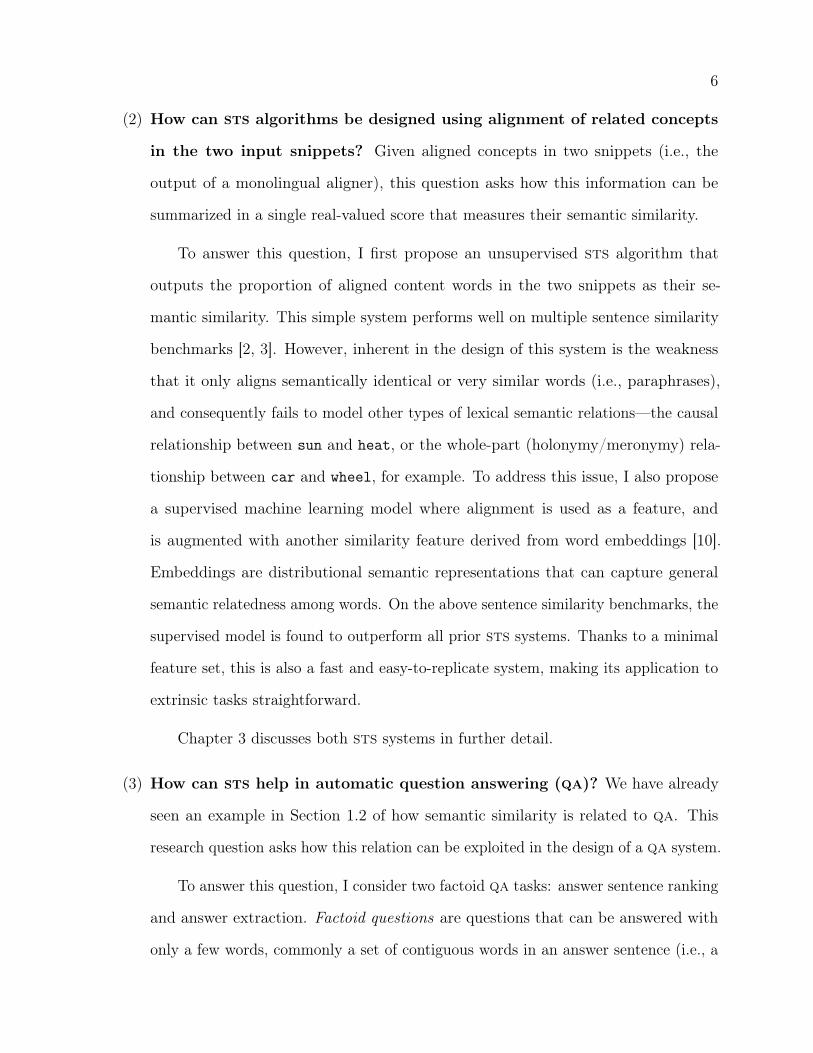
(2) How can sts algorithms be designed using alignment of related concepts

in the two input snippets? Given aligned concepts in two snippets (i.e., the

output of a monolingual aligner), this question asks how this information can be

summarized in a single real-valued score that measures their semantic similarity.

To answer this question, I first propose an unsupervised sts algorithm that

outputs the proportion of aligned content words in the two snippets as their se-

mantic similarity. This simple system performs well on multiple sentence similarity

benchmarks [2, 3]. However, inherent in the design of this system is the weakness

that it only aligns semantically identical or very similar words (i.e., paraphrases),

and consequently fails to model other types of lexical semantic relations—the causal

relationship between sun and heat, or the whole-part (holonymy/meronymy) rela-

tionship between car and wheel, for example. To address this issue, I also propose

a supervised machine learning model where alignment is used as a feature, and

is augmented with another similarity feature derived from word embeddings [10].

Embeddings are distributional semantic representations that can capture general

semantic relatedness among words. On the above sentence similarity benchmarks, the

supervised model is found to outperform all prior sts systems. Thanks to a minimal

feature set, this is also a fast and easy-to-replicate system, making its application to

extrinsic tasks straightforward.

Chapter 3 discusses both sts systems in further detail.

(3) How can sts help in automatic question answering (qa)? We have already

seen an example in Section 1.2 of how semantic similarity is related to qa. This

research question asks how this relation can be exploited in the design of a qa system.

To answer this question, I consider two factoid qa tasks: answer sentence ranking

and answer extraction. Factoid questions are questions that can be answered with

only a few words, commonly a set of contiguous words in an answer sentence (i.e., a

7

chunk); examples include the name of a person, the year of an event, and so on. Given

a question and a set of candidate answer sentences, answer sentence ranking is

the task of assigning each candidate a rank so that the ones that contain an answer

are ranked higher [81, 82, 104, 110]. Answer extraction is the task of extracting

an answer chunk from one or more answer sentences [81, 107].

I develop two different types of models for these tasks. In the first, I follow existing

literature to design a separate model for each. The ranking problem has traditionally

been solved by computing a similarity score for each question-answer sentence pair

and ranking them based on these scores. I design such a supervised ranking model

that learns to assign similarity scores to qa pairs from human annotations. Features

derived from the proposed sts models are used in this model. For extraction, I

compute scores for base noun phrase (np) chunks in a given answer sentence; the

chunks are then assessed by their properties relative to the question (e.g., whether

the question is a who question and the chunk refers to a person).

In the second model type, I propose techniques to combine the outputs of the

two type 1 models above. For answer sentence ranking, this means scoring based

not only on a candidate sentence’s overall similarity with the question but also on

whether it contains the right kind of information to answer the question. Similarly

for answer extraction, this means chunk scoring based not only on a type match with

the question, but also on the relevance of the entire sentence given the question. On

existing qa benchmarks [104, 110], the proposed models outperform current systems

for both extraction and ranking.

A detailed description of these qa systems is provided in Chapter 4.

(4) How can sts help in automatically grading short answers in academic

tests? The example in Table 1.3 shows the relation between text similarity and

student scores in short-answer questions. This research question asks how this relation

8

can be exploited to build automatic short answer graders.

Many existing short answer grading systems operate by computing textual

similarity with the reference answer(s) [44, 51, 68, 77]. I adopt this framework

to design a supervised grader, which employs the feature set of the proposed sts

models and is trained on human-graded short answers. The generic sts features are

also augmented with grading-specific measures: for example, question demoting [68]

proposes to discard words in the answers (both student and reference) that are also

present in the question, since such words are almost never the key answer words that

a grader is looking for. On multiple existing answer grading test sets [31, 68], the

proposed system outperforms existing graders.

The grader is described in Chapter 5.

(5) How can sts algorithms adapt to requirements of different target domains

and applications? The potential applications of sts span a large variety of domains

and applications. For example, the input sentences can come from news headlines,

image captions, tweets, or academic text. We have also seen various applications of

sts in Section 1.2. This question asks how the proposed sts models can adapt to

data from such varied domains and applications.

I explore hierarchical Bayesian domain adaptation [35] to answer this

question. Given training data from different domains and applications, this technique

jointly learns global, domain-, and application-specific instances of the parameters

of a supervised model. At application time, only parameter values specific to the

target domain and application are employed. In my experiments, domain adaptation

improves performance when in-domain training data is scarce.

Domain adaptation is discussed in further detail in Chapter 6.

9

1.4 Contributions

The primary contribution of the research in this dissertation is a set of nlp algorithms

for short-text semantic similarity and related tasks, leading to several publications:

(1) Two top-performing monolingual word aligners that can be applied to text comparison

tasks such as sts, paraphrase detection, and textual entailment recognition; published

in the Transactions of the acl [88] and the Proceedings of emnlp 2015 [92].

(2) Two simple, fast, and state-of-the-art sts systems; published in the Proceedings of

SemEval-2014 [89] and SemEval-2015 [91].

(3) A high-performance joint model for answer sentence ranking and answer extraction;

to be published in the Transactions of the acl [94].

(4) A fast and high-performance short answer grading system; to be published in the

Proceedings of naacl 2016 [95].

(5) An sts model designed to adapt to the requirements of different domains and

applications; to be published in the Proceedings of naacl 2016 [93].

Chapter 2

Monolingual Alignment: Identifying Related Concepts in Short Text Pairs

A central problem underlying short text comparison tasks is that of alignment: pairing

semantic units (i.e. words and phrases) with similar roles in the two input snippets. Such

aligned pairs represent local similarities in the input snippets and can provide useful infor-

mation for sentence-level paraphrase detection, sts and entailment recognition. Alignment

dates back to some of the earliest systems for these tasks [24, 47, 64]. In sts, for example,

information derived from semantically similar or related words in the input snippets has been

utilized by early unsupervised systems [48, 56, 64] as well as recent supervised ones [8, 59, 101].

This high utility has also generated interest in alignment as a standalone task, resulting in

the development of a number of monolingual aligners in recent years [60, 98, 99, 108, 109].

Surprisingly, however, none of these studies explore arguably the simplest and most

intuitive techniques that seem promising for alignment. In this chapter, I identify the core

requirements of alignment, analyze their implications (Sections 2.1 and 2.2), and present

a simple and intuitive design for an unsupervised aligner (Section 2.3). Based on similar

design principles, a supervised model is also proposed (Section 2.4). Experimental results are

presented where both aligners outperform all past systems on multiple benchmarks.

In the context of this dissertation, this chapter explores RQ1 of Section 1.3: How can

semantically similar concepts be identified in a given pair of short text snippets?

11

British 1

armor 2

crashed 3

into 4

a 5

jail 6

to 7

free 8

two 9

soldiers 10

arrested 11

by 12

Iraqi 13

police 14

. 15

1 2 3 4 5 6 7 8 9

Figure 2.1: A human-aligned sentence pair in the msr alignment corpus [16]. The shadedcells depict the alignments, which can also be represented as the set of word index pairs{(1, 1), (2, 2), (3, 3), (4, 3), (5, 4), (6, 5), (6, 6), (13, 8), (15, 9)}. Phrasal alignments are storedas multiple word alignments: (3, 3) and (4, 3) together represent crashed into ↔ stormed.The goal of an aligner is to output this set of pairs.

2.1 The Alignment Problem

Given a short text pair S(1) = (w(1)1 , ..., w

(1)n ) and S(2) = (w

(2)1 , ..., w

(2)m ), where each w is

a word token, the goal of alignment is to generate a (possibly empty) set of token index pairs

{(i, j)} such that w(1)i is aligned to w(2)

j . Figure 2.1 shows an example. This sentence pair is

taken from the msr alignment corpus [16], with related units aligned by human annotators.

The pair (2, 2), for example, indicates that armor in S(1) is aligned to troops in S(2). Phrasal

alignments are represented as sets of index pairs where each token in the S(1) phrase is aligned

to each token in the S(2) phrase. For example, (3, 3) and (4, 3) together in Figure 2.1 encode

12

the alignment crashed into ↔ stormed.

2.2 Alignment: Key Pieces of the Puzzle

An effective aligner can be designed only when the requirements of alignment are clearly

understood. In this section, I illustrate the key pieces of the alignment puzzle using the

sentence pair in Figure 2.1 as an example, and discuss techniques used by existing aligners to

solve them. The term “unit” is used in this section to refer to both words and phrases in a

text snippet.

Evident from the alignments in Figure 2.1 is that aligned units are typically semantically

similar or related. Existing aligners utilize a variety of resources and techniques to identify

semantically similar units, such as WordNet [60, 99], paraphrase databases [109], distributional

similarity measures [60, 109], and string similarity measures [60, 108]. Recent work on neural

word embeddings [10, 65] have advanced the state of distributional similarity, but remain

largely unexplored in the context of monolingual alignment.

Lexical or phrasal similarity alone does not entail alignment, however. Consider function

words: the alignment (5, 4) is present in Figure 2.1 not only because both units are the

word a, but also because they modify semantically equivalent units: jail and police

station. For content word alignment, the influence of context becomes salient particularly

in the presence of competing units. In Figure 2.1, soldiers(10) is not aligned to troops(2)

despite the two words’ semantic equivalence in isolation, due to the presence of a competing

pair, (armor(2), troops(2)), which is a better fit in context.

These examples reveal a second requirement for alignment: assessing the similarity

between the semantic contexts in which the two units appear in their respective snippets.

Most existing aligners employ different contextual similarity measures as features for a

supervised learning model. Such features include shallow surface measures like the difference

in the relative positions of the units being aligned in the respective snippets, and similarities

in the immediate left or right tokens [60, 99, 108]. Deeper syntactic measures like typed

13

dependencies have also been employed as representations of context [98, 99]; these aligners

add constraints for an integer linear program that effectively reward pairs with common

dependencies.

The third and final key component of an aligner is a mechanism to combine lexi-

cal/phrasal and contextual similarities to generate alignments. This task is non-trivial due to

the presence of cooperating and competing units. I first discuss competing units: semantically

similar units in one snippet, each of which is a potential candidate for alignment with one or

more units in the other snippet. At least three different possible scenarios of varying difficulty

exist concerning such units:

• Scenario 1: No competing units. In Figure 2.1, the aligned pair (British(1), UK(1))

represents this scenario.

• Scenario 2: Many-to-one competition—when multiple units in one snippet are similar

to a single unit in the other snippet. In Figure 2.1, (armors(2), troops(2)) and

(soldiers(10), troops(2)) are in such competition.

• Scenario 3: Many-to-many competition—when similar units in one snippet have

multiple potential alignments in the other snippet.

Groups of mutually cooperating units can also exist where one unit provides supporting

evidence for the alignment of other units in the group. Examples (besides multiword

named entities) include individual words in one snippet that are grouped together in the

other snippet (e.g., state of the art ↔ state-of-the-art or headquarters in Paris

↔ Paris-based).

I briefly discuss the working principles of existing aligners to show how they respond to

these challenges. MacCartney et al. [60] and Thadani et al. [98, 99] frame alignment as a set

of phrase edit (insertion, deletion and substitution) operations that transform one snippet into

the other. Each edit operation is scored as a weighted sum of feature values (including lexical

and contextual similarity features), and an optimal set of edits is computed using a decoding

14

algorithm such as simulated annealing [60] or integer linear programming [98, 99]. Yao et

al. [108, 109] take a sequence labeling approach: input snippets are considered sequences of

units and for each unit in one snippet, units in the other snippet are considered potential

labels. A first order conditional random field (crf) is used for prediction.

Only the phrase edit systems above address the challenges posed by competing pairs,

by restricting the participation of each token to exactly one edit. While their phrase-based

representation supports grouping of cooperating tokens in a snippet, use of only lexical

similarity features makes this representation rather ineffective. The sequential model in [109]

allows consecutive tokens to be represented together in a single semi-Markovian state, which

are matched to tokens and phrases in the other snippet using the ppdb phrasal paraphrases

[37].

2.3 Unsupervised Alignment Using Lexical and Contextual Similarity

It can be argued that existing aligners, while important and interesting in their approach,

emphasize more on elegant mathematical modeling than on addressing the central challenges

of alignment. For example, while sequential models are more powerful than individual

token-based models, it is not clear how much an aligner gains by just using a first-order

crf as in [108, 109], and ignoring deeper and longer-distance contextual features such as

typed dependencies. Furthermore, replication of such systems is fairly difficult, limiting their

usability in downstream applications.

In view of the above, I propose a lightweight, easy-to-construct aligner that produces

high-quality output. The basic idea is to treat alignment as a weighted bipartite matching

problem, where weights of word token pairs (w(1)i , w

(2)j ) ∈ S(1)×S(2) are derived via simple and

intuitive application of robust linguistic representations of lexical and contextual similarity. I

primarily focus on word alignment, which Yao et al. [109] report to cover more than 95% of

all alignments in multiple human-annotated corpora [16, 98]. This aligner has been made

15

Alignidenticalword

sequences

Alignnamedentities

Aligncontentwords

Alignstopwords

Figure 2.2: Unsupervised alignment pipeline.

open-source.1

2.3.1 System Description

This system operates as a pipeline of alignment modules, each of which aligns a unique

type of word pair. Figure 2.2 shows a block diagram, where each rectangle represents a

module. Each module makes use of contextual evidence to make alignment decisions. In

addition, the last two modules utilize a lexical semantic similarity resource. Because of their

phrasal nature, it treats named entities separately from other content words. The rationale

behind the order in which the modules are arranged is discussed later in this section.

Before discussing each alignment module in detail, I describe the system components

that identify lexical and contextual similarity.

2.3.1.1 Lexical Similarity

The ability to correctly identify lexical semantic similarity is key for any aligner, as

pointed out in Section 2.2. Instead of treating lexical similarity as a continuous variable, I

define a coarser-grained three-level measure of similarity.

The first level is an exact word or lemma match which is represented by a similarity

score of 1. The second level represents non-identical but semantically similar terms. To

identify such word pairs, I use the Paraphrase Database (ppdb) [37]—a large resource of

lexical and phrasal paraphrases constructed using bilingual pivoting [7] over large parallel

1https://github.com/ma-sultan/monolingual-word-aligner

16

corpora. I use the largest (xxxl) of the ppdb’s lexical paraphrase packages and treat all pairs

identically by ignoring the accompanying statistics. The resource is customized by removing

pairs of identical words or lemmas and adding lemmatized forms of the remaining pairs. For

now, I use the term ppdbSim to refer to the similarity of each word pair in this modified

version of ppdb (which is a value in (0, 1)) and later explain how the system determines it

(Section 2.3.1.3). Finally, any pair of different words which is also absent in ppdb is assigned

a zero similarity score.

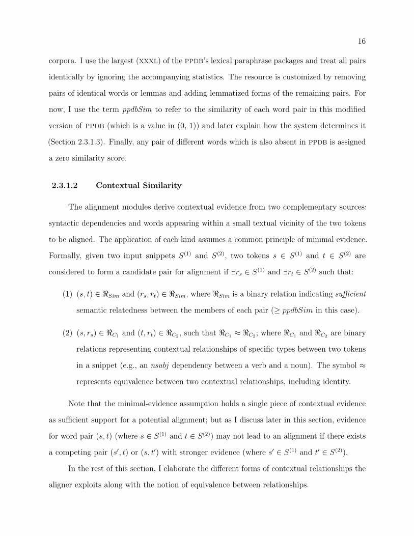
2.3.1.2 Contextual Similarity

The alignment modules derive contextual evidence from two complementary sources:

syntactic dependencies and words appearing within a small textual vicinity of the two tokens

to be aligned. The application of each kind assumes a common principle of minimal evidence.

Formally, given two input snippets S(1) and S(2), two tokens s ∈ S(1) and t ∈ S(2) are

considered to form a candidate pair for alignment if ∃rs ∈ S(1) and ∃rt ∈ S(2) such that:

(1) (s, t) ∈ <Sim and (rs, rt) ∈ <Sim, where <Sim is a binary relation indicating sufficient

semantic relatedness between the members of each pair (≥ ppdbSim in this case).

(2) (s, rs) ∈ <C1 and (t, rt) ∈ <C2 , such that <C1 ≈ <C2 ; where <C1 and <C2 are binary

relations representing contextual relationships of specific types between two tokens

in a snippet (e.g., an nsubj dependency between a verb and a noun). The symbol ≈

represents equivalence between two contextual relationships, including identity.

Note that the minimal-evidence assumption holds a single piece of contextual evidence

as sufficient support for a potential alignment; but as I discuss later in this section, evidence

for word pair (s, t) (where s ∈ S(1) and t ∈ S(2)) may not lead to an alignment if there exists

a competing pair (s′, t) or (s, t′) with stronger evidence (where s′ ∈ S(1) and t′ ∈ S(2)).

In the rest of this section, I elaborate the different forms of contextual relationships the

aligner exploits along with the notion of equivalence between relationships.

17

S(1): He wrote a book .

nsubj

dobj

det

S(2): I read the book he wrote .

nsubj

dobj

det

rcmod

nsubj

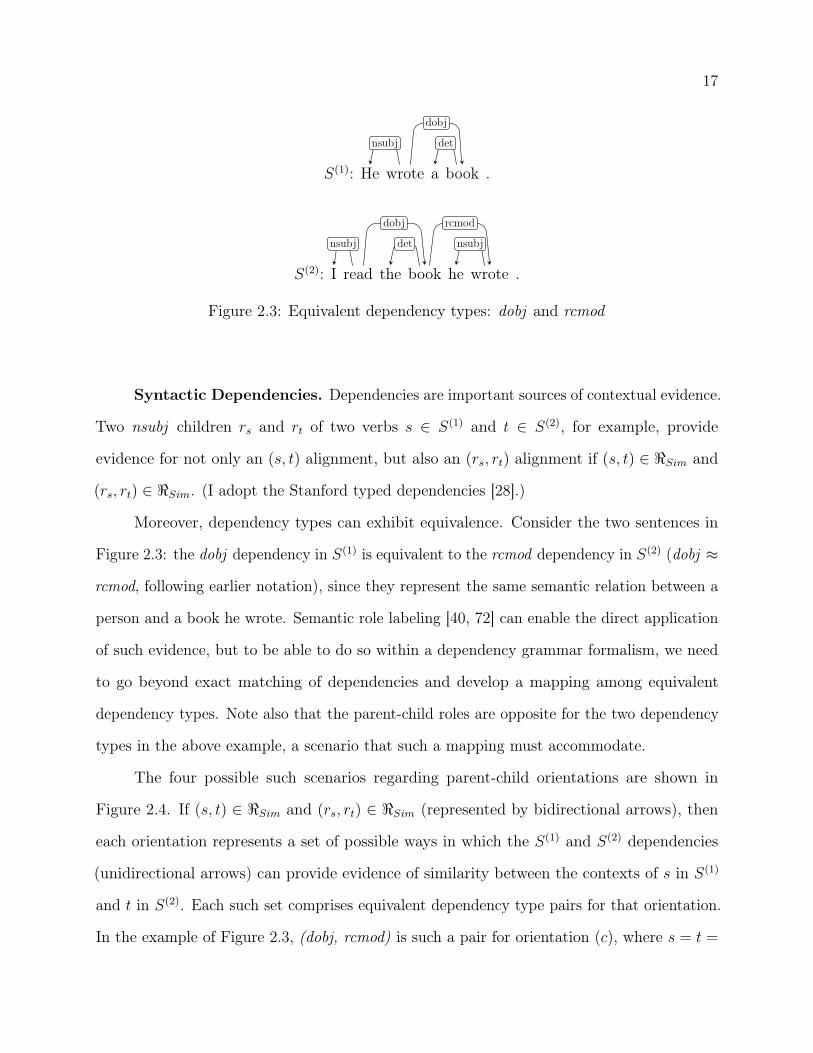
Figure 2.3: Equivalent dependency types: dobj and rcmod

Syntactic Dependencies. Dependencies are important sources of contextual evidence.

Two nsubj children rs and rt of two verbs s ∈ S(1) and t ∈ S(2), for example, provide

evidence for not only an (s, t) alignment, but also an (rs, rt) alignment if (s, t) ∈ <Sim and

(rs, rt) ∈ <Sim. (I adopt the Stanford typed dependencies [28].)

Moreover, dependency types can exhibit equivalence. Consider the two sentences in

Figure 2.3: the dobj dependency in S(1) is equivalent to the rcmod dependency in S(2) (dobj ≈

rcmod, following earlier notation), since they represent the same semantic relation between a

person and a book he wrote. Semantic role labeling [40, 72] can enable the direct application

of such evidence, but to be able to do so within a dependency grammar formalism, we need

to go beyond exact matching of dependencies and develop a mapping among equivalent

dependency types. Note also that the parent-child roles are opposite for the two dependency

types in the above example, a scenario that such a mapping must accommodate.

The four possible such scenarios regarding parent-child orientations are shown in

Figure 2.4. If (s, t) ∈ <Sim and (rs, rt) ∈ <Sim (represented by bidirectional arrows), then

each orientation represents a set of possible ways in which the S(1) and S(2) dependencies

(unidirectional arrows) can provide evidence of similarity between the contexts of s in S(1)

and t in S(2). Each such set comprises equivalent dependency type pairs for that orientation.

In the example of Figure 2.3, (dobj, rcmod) is such a pair for orientation (c), where s = t =

18

s

rs

t

rt

rs

s

rt

t

s

rs

t

rt

s

rs

t

rt

(a) (b) (c) (d)

Figure 2.4: Parent-child orientations in dependencies.

wrote and rs = rt = book.

I apply the notion of dependency type equivalence to intra-category alignment of content

words in four major lexical categories: verbs, nouns, adjectives and adverbs (the Stanford pos

tagger [100] is used to identify the categories). Table 2.1 shows dependency type equivalences

for each lexical category of s and t.

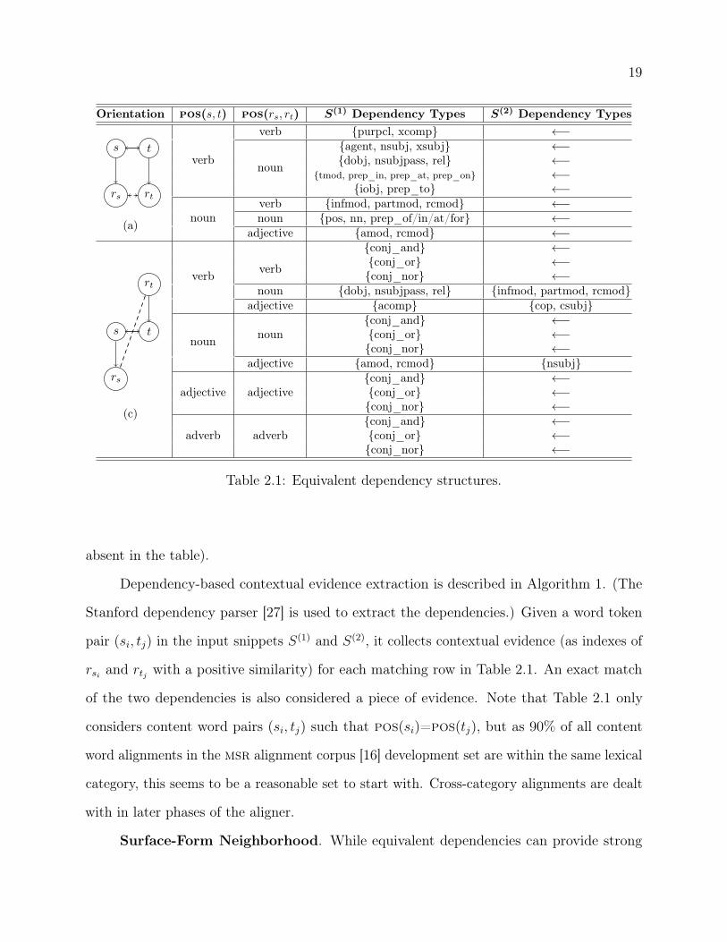
The ‘←’ sign on column 5 of some rows represents a duplication of the column 4 content

of the same row. For each row, columns 4 and 5 show two sets of dependency types; each

member of the first is equivalent to each member of the second for the current orientation

(column 1) and lexical categories of the associated words (columns 2 and 3). For example, row

2 represents the fact that an agent relation (between s and rs; s is the parent) is equivalent

to an nsubj relation (between t and rt; t is the parent).

Note that the equivalences are fundamentally redundant across different orientations.

For example, row 2 (which is presented as an instance of orientation (a) can also be presented

as an instance of orientation (b) with pos(s)=pos(t)=noun and pos(rs)=pos(rt)=verb. Such

redundant equivalences are not shown in the table. As another example, the equivalence of

dobj and rcmod in Figure 2.3 is shown in the table only as an instance of orientation (c) and

not as an instance of orientation (d). (In general, this is why orientations (b) and (d) are

19

Orientation pos(s, t) pos(rs, rt) S(1) Dependency Types S(2) Dependency Types

s

rs

t

rt

verb

verb {purpcl, xcomp} ←−

noun

{agent, nsubj, xsubj} ←−{dobj, nsubjpass, rel} ←−

{tmod, prep_in, prep_at, prep_on} ←−{iobj, prep_to} ←−

nounverb {infmod, partmod, rcmod} ←−

(a) noun {pos, nn, prep_of/in/at/for} ←−adjective {amod, rcmod} ←−

s

rs

t

rtverb verb

{conj_and} ←−{conj_or} ←−{conj_nor} ←−

noun {dobj, nsubjpass, rel} {infmod, partmod, rcmod}adjective {acomp} {cop, csubj}

noun noun{conj_and} ←−{conj_or} ←−{conj_nor} ←−

adjective {amod, rcmod} {nsubj}

adjective adjective{conj_and} ←−{conj_or} ←−

(c) {conj_nor} ←−

adverb adverb{conj_and} ←−{conj_or} ←−{conj_nor} ←−

Table 2.1: Equivalent dependency structures.

absent in the table).

Dependency-based contextual evidence extraction is described in Algorithm 1. (The

Stanford dependency parser [27] is used to extract the dependencies.) Given a word token

pair (si, tj) in the input snippets S(1) and S(2), it collects contextual evidence (as indexes of

rsi and rtj with a positive similarity) for each matching row in Table 2.1. An exact match

of the two dependencies is also considered a piece of evidence. Note that Table 2.1 only

considers content word pairs (si, tj) such that pos(si)=pos(tj), but as 90% of all content

word alignments in the msr alignment corpus [16] development set are within the same lexical

category, this seems to be a reasonable set to start with. Cross-category alignments are dealt

with in later phases of the aligner.

Surface-Form Neighborhood. While equivalent dependencies can provide strong

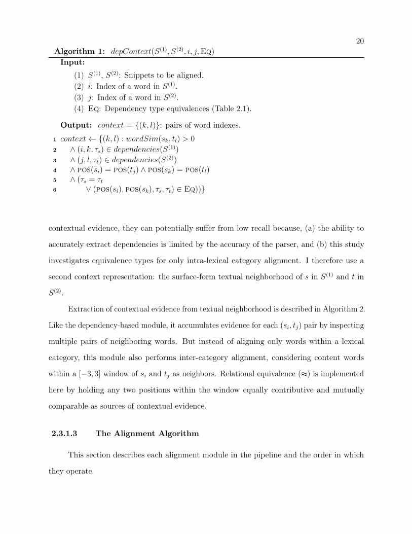
20Algorithm 1: depContext(S(1), S(2), i, j,Eq)

Input:

(1) S(1), S(2): Snippets to be aligned.(2) i: Index of a word in S(1).(3) j: Index of a word in S(2).(4) Eq: Dependency type equivalences (Table 2.1).

Output: context = {(k, l)}: pairs of word indexes.

1 context← {(k, l) : wordSim(sk, tl) > 0

2 ∧ (i, k, τs) ∈ dependencies(S(1))

3 ∧ (j, l, τt) ∈ dependencies(S(2))4 ∧ pos(si) = pos(tj) ∧ pos(sk) = pos(tl)5 ∧ (τs = τt6 ∨ (pos(si),pos(sk), τs, τt) ∈ Eq))}

contextual evidence, they can potentially suffer from low recall because, (a) the ability to

accurately extract dependencies is limited by the accuracy of the parser, and (b) this study

investigates equivalence types for only intra-lexical category alignment. I therefore use a

second context representation: the surface-form textual neighborhood of s in S(1) and t in

S(2).

Extraction of contextual evidence from textual neighborhood is described in Algorithm 2.

Like the dependency-based module, it accumulates evidence for each (si, tj) pair by inspecting

multiple pairs of neighboring words. But instead of aligning only words within a lexical

category, this module also performs inter-category alignment, considering content words

within a [−3, 3] window of si and tj as neighbors. Relational equivalence (≈) is implemented

here by holding any two positions within the window equally contributive and mutually

comparable as sources of contextual evidence.

2.3.1.3 The Alignment Algorithm

This section describes each alignment module in the pipeline and the order in which

they operate.

21Algorithm 2: textContext(S(1), S(2), i, j,Stop)

Input:

(1) S(1), S(2): Snippets to be aligned.(2) i: Index of a word in S(1).(3) j: Index of a word in S(2).(4) Stop: A set of stop words.

Output: context = {(k, l)}: pairs of word indexes.

1 Ci ← {k : k ∈ [i− 3, i+ 3] ∧ k 6= i ∧ sk 6∈ Stop}2 Cj ← {l : l ∈ [j − 3, j + 3] ∧ l 6= j ∧ tl 6∈ Stop}3 context← Ci × Cj

Identical Word Sequences. The presence of a common word sequence in S(1) and

S(2) is indicative of an (a) identical, and (b) contextually similar word in the other sentence

for each word in the sequence. On the msr alignment corpus [16] dev set, one-to-one

alignment of tokens in such sequences of length n demonstrates a high precision (≈ 97%) for

n ≥ 2. Thus membership in such sequences can be considered a simple form of contextual

evidence for alignment; the proposed aligner aligns all identical word sequence pairs in S(1)

and S(2) containing at least one content word. From here on, I will refer to this module as

wordSequenceAlign.

A special case of sequences aligned in this manner is a hyphen-delimited group of tokens

that appears in the other snippet as individual tokens (e.g., state-of-the-art ↔ state of

the art). Note that this is a form of cooperation among tokens in the latter snippet.

Named Entities. Named entities are aligned separately to enable the alignment of

full and partial mentions (and acronyms) of the same entity. Note that tokens in the full

mention in such cases are mutually cooperating. The Stanford Named Entity Recognizer [34]

is used to identify named entities in S(1) and S(2). After aligning the exact term matches, any

unmatched term of a partial mention is aligned to all terms in the full mention. The module

recognizes only first-letter acronyms (e.g., NYC: New York City) and aligns an acronym to

all terms in the full mention of the corresponding name.

22

Since named entities are instances of nouns, named entity alignment is also informed by

contextual evidence like any other content word (which I discuss next), but happens before

alignment of other generic content words. Parents (or children) of a named entity are simply

the parents (or children) of its head word. I will refer to this module as a method named

namedEntityAlign from this point on.

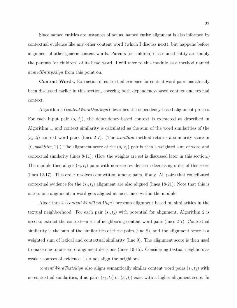
Content Words. Extraction of contextual evidence for content word pairs has already

been discussed earlier in this section, covering both dependency-based context and textual

context.

Algorithm 3 (contentWordDepAlign) describes the dependency-based alignment process.

For each input pair (si, tj), the dependency-based context is extracted as described in

Algorithm 1, and context similarity is calculated as the sum of the word similarities of the

(sk, tl) context word pairs (lines 2-7). (The wordSim method returns a similarity score in

{0, ppdbSim, 1}.) The alignment score of the (si, tj) pair is then a weighted sum of word and

contextual similarity (lines 8-11). (How the weights are set is discussed later in this section.)

The module then aligns (si, tj) pairs with non-zero evidence in decreasing order of this score

(lines 12-17). This order resolves competition among pairs, if any. All pairs that contributed

contextual evidence for the (si, tj) alignment are also aligned (lines 18-21). Note that this is

one-to-one alignment: a word gets aligned at most once within the module.

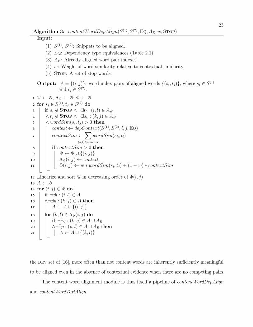
Algorithm 4 (contentWordTextAlign) presents alignment based on similarities in the

textual neighborhood. For each pair (si, tj) with potential for alignment, Algorithm 2 is

used to extract the context—a set of neighboring content word pairs (lines 2-7). Contextual

similarity is the sum of the similarities of these pairs (line 8), and the alignment score is a

weighted sum of lexical and contextual similarity (line 9). The alignment score is then used

to make one-to-one word alignment decisions (lines 10-15). Considering textual neighbors as

weaker sources of evidence, I do not align the neighbors.

contentWordTextAlign also aligns semantically similar content word pairs (si, tj) with

no contextual similarities, if no pairs (sk, tj) or (si, tl) exist with a higher alignment score. In

23Algorithm 3: contentWordDepAlign(S(1), S(2),Eq, AE, w,Stop)

Input:

(1) S(1), S(2): Snippets to be aligned.(2) Eq: Dependency type equivalences (Table 2.1).(3) AE: Already aligned word pair indexes.(4) w: Weight of word similarity relative to contextual similarity.(5) Stop: A set of stop words.

Output: A = {(i, j)}: word index pairs of aligned words {(si, tj)}, where si ∈ S(1)

and tj ∈ S(2).

1 Ψ← ∅; ΛΨ ← ∅; Φ← ∅2 for si ∈ S(1), tj ∈ S(2) do3 if si 6∈ Stop ∧ ¬∃tl : (i, l) ∈ AE4 ∧ tj 6∈ Stop ∧ ¬∃sk : (k, j) ∈ AE5 ∧ wordSim(si, tj) > 0 then6 context← depContext(S(1), S(2), i, j,Eq)

7 contextSim←∑

(k,l)∈context

wordSim(sk, tl)

8 if contextSim > 0 then9 Ψ← Ψ ∪ {(i, j)}

10 ΛΨ(i, j)← context11 Φ(i, j)← w ∗ wordSim(si, tj) + (1− w) ∗ contextSim

12 Linearize and sort Ψ in decreasing order of Φ(i, j)13 A← ∅14 for (i, j) ∈ Ψ do15 if ¬∃l : (i, l) ∈ A16 ∧¬∃k : (k, j) ∈ A then17 A← A ∪ {(i, j)}18 for (k, l) ∈ ΛΨ(i, j) do19 if ¬∃q : (k, q) ∈ A ∪ AE20 ∧¬∃p : (p, l) ∈ A ∪ AE then21 A← A ∪ {(k, l)}

the dev set of [16], more often than not content words are inherently sufficiently meaningful

to be aligned even in the absence of contextual evidence when there are no competing pairs.

The content word alignment module is thus itself a pipeline of contentWordDepAlign

and contentWordTextAlign.

24Algorithm 4: contentWordTextAlign(S(1), S(2), AE, w,Stop)

Input:

(1) S(1), S(2): Snippets to be aligned.(2) AE: Existing alignments by word indexes.(3) w: Weight of word similarity relative to contextual similarity.(4) Stop: A set of stop words.

Output: A = {(i, j)}: word index pairs of aligned words {(si, tj)}, where si ∈ S(1)

and tj ∈ S(2).

1 Ψ← ∅; Φ← ∅2 for si ∈ S(1), tj ∈ S(2) do3 if si 6∈ Stop ∧ ¬∃tl : (i, l) ∈ AE4 ∧ tj 6∈ Stop ∧ ¬∃sk : (k, j) ∈ AE5 ∧ wordSim(si, tj) > 0 then6 Ψ← Ψ ∪ {(i, j)}7 context← textContext(S(1), S(2), i, j,Stop)

8 contextSim←∑

(k,l)∈context

wordSim(sk, tl)

9 Φ(i, j)← w ∗ wordSim(si, tj) + (1− w) ∗ contextSim

10 Linearize and sort Ψ in decreasing order of Φ(i, j)11 A← ∅12 for (i, j) ∈ Ψ do13 if ¬∃l : (i, l) ∈ A14 ∧¬∃k : (k, j) ∈ A then15 A← A ∪ {(i, j)}

Stop Words. Some stop words get aligned by the aligner as part of identical word

sequence alignment and neighbor alignment as discussed earlier in this section. For the

rest, dependencies and surface-form textual neighborhoods are used as before, with three

adjustments.

First, since stop word alignment is the last step in the pipeline, only pairs that have

already been aligned are considered to provide contextual evidence—other pairs have already

been judged unrelated by the aligner regardless of their degree of lexical and contextual

similarity. Second, since many stop words (e.g. determiners, modals) typically demonstrate

little variation in the dependencies they engage in, I ignore type equivalences for stop words

25Algorithm 5: align(S(1), S(2),Eq, w,Stop)

Input:

(1) S(1), S(2): Snippets to be aligned.(2) Eq: Dependency type equivalences (Table 2.1).(3) w: Weight of lexical similarity relative to contextual similarity.(4) Stop: A set of stop words.

Output: A = {(i, j)}: word index pairs of aligned words {(si, tj)} where si ∈ S(1) andtj ∈ S(2).

1 A← wordSequenceAlign(S(1), S(2))

2 A← A ∪ namedEntityAlign(S(1), S(2),Eq, A, w)

3 A← A ∪ contentWordDepAlign(S(1), S(2),Eq, A, w,Stop)

4 A← A ∪ contentWordTextAlign(S(1), S(2), A, w,Stop)

5 A← A ∪ stopWordDepAlign(S(1), S(2), A, w,Stop)

6 A← A ∪ stopWordTextAlign(S(1), S(2), A, w,Stop)

and implement only exact matching of dependencies.2 Finally, for textual neighborhood, the

aligner disregards alignment of left neighbors of one word with right neighbors of the other

and vice versa—again due to the relatively fixed nature of dependencies between stop words

and their neighbors.

Thus stop words are also aligned in a sequence of dependency and textual neighborhood-

based alignments. I assume two corresponding modules named stopWordDepAlign and

stopWordTextAlign, respectively.

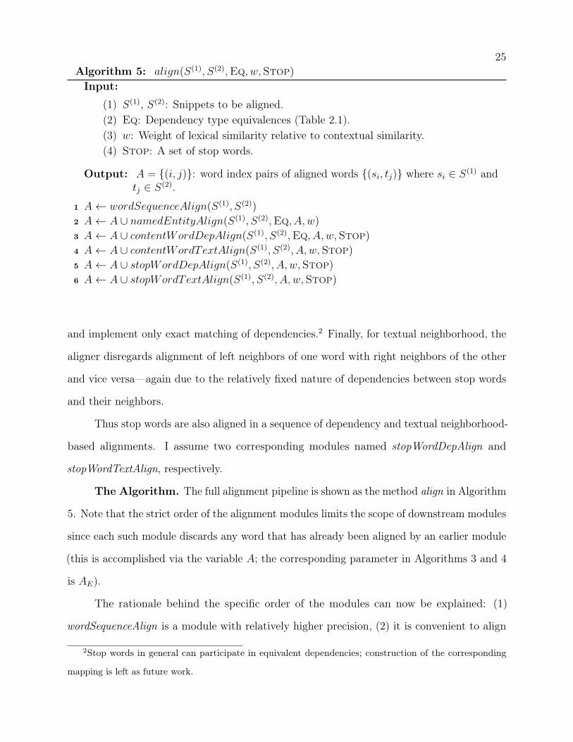
The Algorithm. The full alignment pipeline is shown as the method align in Algorithm

5. Note that the strict order of the alignment modules limits the scope of downstream modules

since each such module discards any word that has already been aligned by an earlier module

(this is accomplished via the variable A; the corresponding parameter in Algorithms 3 and 4

is AE).

The rationale behind the specific order of the modules can now be explained: (1)

wordSequenceAlign is a module with relatively higher precision, (2) it is convenient to align

2Stop words in general can participate in equivalent dependencies; construction of the corresponding

mapping is left as future work.

26

named entities before other content words to enable alignment of entity mentions of different

lengths, (3) dependency-based evidence was observed to be more reliable (i.e. of higher

precision) than surface-form textual evidence in the msr alignment corpus dev set, and (4)

stop word alignments are dependent on existing content word alignments.

The aligner assumes two free parameters: ppdbSim and w (in Algorithms 3 and 4). To

determine their values, an exhaustive grid search is performed through the two-dimensional

space (ppdbSim,w) for ppdbSim,w ∈ {0.1, 0.2, ..., 0.9, 1}, and the combination (0.9, 0.9)

yields the best F1 score on the msr corpus dev set. While this adds a minimal amount of

supervision to the design of the aligner, these values are used unchanged in all subsequent

applications of the aligner reported in this dissertation (i.e. without any retraining).

2.3.2 Evaluation

I evaluate the proposed aligner both intrinsically and extrinsically on multiple corpora.

This section discusses the results.

2.3.2.1 Intrinsic Evaluation

The msr alignment dataset3 [16] provides annotations for training and intrinsically

evaluating monolingual aligners. Three annotators individually aligned words and phrases

in 1,600 pairs of premise and hypothesis sentences from the rte2 challenge data (divided

into dev and test sets, each consisting of 800 sentences). The dataset has subsequently

been used to evaluate several top performing aligners [60, 99, 108, 109]. I use the test set

for evaluation; following the above studies, (a) a majority rule is applied to select from the

three sets of annotations for each sentence and discard three-way disagreements, (b) only the

sure links are used (word pairs that annotators mentioned should certainly be aligned, as

opposed to possible links).

I test the generalizability of the aligner by evaluating it, unchanged (i.e. with identical

3http://www.cs.biu.ac.il/~nlp/files/RTE_2006_Aligned.zip

27

System P% R% F1% E%

msr

MacCartney et al. [60] 85.4 85.3 85.3 21.3Thadani & McKeown [99] 89.5 86.2 87.8 33.0Yao et al. [108] 93.7 84.0 88.6 35.3Yao et al. [109] 92.1 82.8 86.8 29.1This Aligner 93.7 89.8 91.7 43.8

edb

++ Yao et al. [108] 91.3 82.0 86.4 15.0

Yao et al. [109] 90.4 81.9 85.9 13.7This Aligner 93.5 82.5 87.6 18.3

Table 2.2: Results of intrinsic evaluation on two datasets.

parameter values), on a second alignment corpus: the Edinburgh++4 [98] corpus. The test

set consists of 306 pairs; each pair is aligned by at most two annotators, and I adopt the

random selection policy described in [98] to resolve disagreements.

Table 2.2 shows the results. For each corpus, it shows precision (% system alignments

that match gold annotations), recall (% gold alignments discovered by the aligner), F1 score

and the percentage of sentences that receive the exact gold alignments (denoted by E) from

the aligner.

On the msr test set, the proposed aligner shows a 3.1% improvement in F1 score over

the previous best system [108] with a 27.2% error reduction. Importantly, it demonstrates

a considerable increase in recall without any loss in precision. The E score also increases

as a consequence. On the Edinburgh++ test set, the proposed aligner achieves a 1.2%

increase in F1 score (an error reduction of 8.8%) over the previous best system [108], with

improvements in both precision and recall.

2.3.2.2 Ablation Test

Ablation tests are run to assess the importance of the aligner’s individual components.

Each row in Table 2.3 beginning with (-) shows a feature excluded from the aligner and two

4http://www.ling.ohio-state.edu/~scott/#edinburgh-plusplus

28

msr edb++

Feature P% R% F1% P% R% F1%

Original 93.7 89.8 91.7 93.5 82.5 87.6(-) Word Similarity 95.2 86.3 90.5 95.1 77.3 85.3(-) Contextual Evidence 81.3 86.0 83.6 86.4 80.6 83.4(-) Dependencies 94.2 88.8 91.4 93.8 81.3 87.1(-) Text Neighborhood 85.5 90.4 87.9 90.4 84.3 87.2

Table 2.3: Ablation test results.

associated sets of metrics, showing the performance of the resulting algorithm on the two

alignment corpora.

Without a word similarity module, recall drops as expected. Without contextual

evidence (word sequences, dependencies and textual neighbors) precision drops considerably

and recall also falls. Without dependencies, the aligner still gives state-of-the-art results,

which points to the possibility of a very fast yet high-performance aligner. Without evidence

from surface-form textual neighbors, however, the precision of the aligner suffers badly.

Textual neighbors find alignments across different lexical categories, a type of alignment that

is currently not supported by the dependency equivalences. Extending the set of dependency

type equivalences might alleviate this issue.

2.3.2.3 Error Analysis

To better understand the failure modes of the aligner, I examine its performance on

different types of word pairs. Each token is first categorized along two different dimensions:

(1) whether or not it is part of a named entity, and (2) which of the following groups it

belongs to: content words, function words, and punctuation marks. Combined, these two

dimensions form a domain of six possible values which can be represented as the Cartesian

product {non-named entity, named entity} × {content word, function word, punctuation

mark}. Each member of this set is a word type in this experiment; for instance, named entity

29

05101520253035404550

{nne-c, nne-c}

{nne-c, nne-f}

{nne-c, ne-c}

{nne-f, nne-f}

{nne-p, nne-p}

{ne-c, ne-c}

MSR EDB++

Figure 2.5: % distribution of aligned word pair types; nne: non-named entity, ne: namedentity, c: content word, f : function word, p: punctuation mark.

function word is a word type.

Given input snippets S(1) and S(2), the notion of types is then extended to word pairs in

S(1) × S(2): the type of pair (w(1)i , w

(2)j ) is the union of the types of w(1)

i and w(2)j . Figure 2.5

shows the % distribution of word pair types with at least 20 aligned instances in at least one

test set. These six types account for more than 99% of all alignments in both test sets.

Table 2.4 shows performance on each of these six word pair types. Performance is good

overall, except on {nne-c, nne-f } pairs. These pairs are intrinsically difficult for a word aligner

because they occur frequently as part of phrasal alignments, e.g., the pair (into, stormed)

in Figure 2.1 where the phrase crashed into was aligned to the word stormed. Recall is

also relatively low on {nne-c, ne-c} pairs; on many occasions, world knowledge is required

to recognize their semantic equivalence (e.g., in daughter ↔ Chelsea, or California ↔

state). Fortunately, these two word pair types are the least common of the six in both test

sets, indicating their overall low frequency.

Some false negatives are found in {nne-c, nne-c} pairs as well, due primarily to (1)

use of ppdb as the only lexical similarity resource, and (2) failure to address one-to-many

alignments. This also has an effect on {nne-f, nne-f } pairs, as function word alignment is

dependent on related content word alignment.

30

msr edb++

Pair Type P% R% F1% P% R% F1%{nne-c, nne-c} 93.4 85.2 89.1 92.7 87.0 89.8{nne-c, nne-f } 100.0 1.4 2.7 88.9 4.2 8.0{nne-c, ne-c} 87.1 82.2 84.6 75.9 68.8 72.1{nne-f, nne-f } 86.5 88.4 87.4 95.3 82.5 88.4{nne-p, nne-p} 99.5 99.4 99.5 96.3 91.3 93.8{ne-c, ne-c} 95.8 97.4 96.6 93.8 91.6 92.7

Table 2.4: Performance on different word pair types.

2.3.2.4 Extrinsic Evaluation

The aligner is extrinsically evaluated on short text similarity and paraphrase detection.

Short Text Similarity (sts). In the context of this dissertation, sts is the primary

target task for the aligner. Chapter 3 explores sts via alignment in greater detail; here I run a

short experiment to extrinsically evaluate the aligner. The setup and test data are taken from

the SemEval-2013 Semantic Textual Similarity task [3]. There are four test datasets in the

SemEval-2013 sts corpus, each containing sentence pairs with associated human annotations

of similarity. The Pearson product-moment correlation coefficient (Pearson’s r) with human

annotations is computed individually for each test set and a weighted sum of the correlations

is used as the final evaluation metric. The weight of a test set is proportional to the number

of pairs it contains.

The aligner is applied to the task by aligning each sentence pair and taking the

proportion of content words aligned in the two sentences (by normalizing with the harmonic

mean of their number of content words) as a proxy of their semantic similarity. Only three

of the four SemEval-2013 sts datasets were freely available at the time of this experiment

(Headlines, Onwn, and fnwn),5 and are used here (leaving out the smt dataset). These

three sets contain 1500 annotated sentence pairs in total.

5http://ixa2.si.ehu.es/sts/

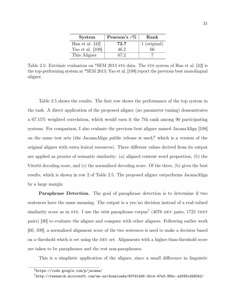
31

System Pearson’s r% RankHan et al. [42] 73.7 1 (original)Yao et al. [108] 46.2 66This Aligner 67.2 7

Table 2.5: Extrinsic evaluation on *SEM 2013 sts data. The sts system of Han et al. [42] isthe top-performing system at *SEM 2013; Yao et al. [108] report the previous best monolingualaligner.

Table 2.5 shows the results. The first row shows the performance of the top system in

the task. A direct application of the proposed aligner (no parameter tuning) demonstrates

a 67.15% weighted correlation, which would earn it the 7th rank among 90 participating

systems. For comparison, I also evaluate the previous best aligner named JacanaAlign [108]

on the same test sets (the JacanaAlign public release is used,6 which is a version of the

original aligner with extra lexical resources). Three different values derived from its output

are applied as proxies of semantic similarity: (a) aligned content word proportion, (b) the

Viterbi decoding score, and (c) the normalized decoding score. Of the three, (b) gives the best

results, which is shown in row 2 of Table 2.5. The proposed aligner outperforms JacanaAlign

by a large margin.

Paraphrase Detection. The goal of paraphrase detection is to determine if two

sentences have the same meaning. The output is a yes/no decision instead of a real-valued

similarity score as in sts. I use the msr paraphrase corpus7 (4076 dev pairs, 1725 test

pairs) [30] to evaluate the aligner and compare with other aligners. Following earlier work

[60, 109], a normalized alignment score of the two sentences is used to make a decision based

on a threshold which is set using the dev set. Alignments with a higher-than-threshold score

are taken to be paraphrases and the rest non-paraphrases.

This is a simplistic application of the aligner, since a small difference in linguistic

6https://code.google.com/p/jacana/7http://research.microsoft.com/en-us/downloads/607d14d9-20cd-47e3-85bc-a2f65cd28042/

32

System Accuracy% P% R% F1%

Madnani et al. [61] 77.4 79.0 89.9 84.1Yao et al. [108] 70.0 72.6 88.1 79.6Yao et al. [109] 68.1 68.6 95.8 79.9This Aligner 73.4 76.6 86.4 81.2

Table 2.6: Extrinsic evaluation on msr paraphrase data. Madnani et al. [42] have the bestperformance on this dataset; Yao et al. [108, 109] report state-of-the-art monolingual aligners.

properties of two sentences (e.g. polarity or modality) can make them non-paraphrases

despite a high degree of alignment. So the aligner was not expected to demonstrate state-of-

the-art performance, but still it gets close, as shown in Table 2.6. The first column shows

the accuracy of each system in classifying the input sentences into one of two classes: true

(paraphrases) and false (non-paraphrases). The rest of the columns show the performance of

the system for the true class in terms of precision, recall, and F1 score. Italicized numbers

represent scores that were not reported by the authors of the corresponding papers, but are

reconstructed from the reported data (and hence are likely to have small precision errors).

The first row shows the best performance by any system on this test set at the time of

this experiment. The next two rows show the performance of two state-of-the-art aligners

(performances of both systems were reported in [109]). The last row shows the performance of

the proposed aligner. Although it does worse than the best paraphrase system, it outperforms

the other aligners.

2.3.3 Discussion

The above results show that a word aligner based on simple measures of lexical and

contextual similarity can demonstrate state-of-the-art accuracy. However, as aligners are

frequently components of larger systems, accuracy is not always the only concern. Other

dimensions of an aligner’s usefulness include speed, consumption of computing resources,

33

replicability, and generalizability to different applications. My design goals include achieving

a balance among such multifarious and conflicting goals.

A speed advantage of the proposed aligner stems from framing the problem as one-to-one

word alignment and thus avoiding an expensive decoding phase. The presence of multiple

phases is offset by discarding already aligned words in subsequent phases. The use of ppdb as

the only lexical similarity resource helps in reducing latency as well as space requirements. As

shown in the ablation study, further speedup could be achieved with only a small performance

degradation by considering only the textual neighborhood as source of contextual evidence.

However, the two major goals that the aligner arguably achieves to the greatest extent

are replicability and generalizability. Easy replicability of the aligner stems from its use of

only basic and frequently used nlp modules (a lemmatizer, a pos tagger, an ner module,

and a dependency parser for English: all available as part of the Stanford Corenlp suite;8 I

use a Python wrapper9) and a single lexical similarity resource (ppdb).

The aligner demonstrates top performance in both intrinsic and extrinsic evaluation. A

design characteristic that enhances the generalizability of the aligner is its minimal dependence

on the msr alignment training data, which originates from a textual entailment corpus having

unique properties such as disparities in the lengths of the input sentences and a directional

nature of their relationship (i.e., the premise implying the hypothesis, but not vice versa). A

related potential reason is the symmetry of the aligner’s output (caused by its assumption of

no directionality)—the fact that it outputs the same set of alignments regardless of the order

of the input sentences, in contrast to most existing aligners.

Major limitations of the aligner include the inability to align phrases, including multiword

expressions. It is incapable of capturing and exploiting long-distance relations among words

in a snippet. It uses ppdb as the only resource to identify paraphrases; but no resource

is perfect and ppdb is no exception, therefore some related word pairs remain unaligned.

8http://stanfordnlp.github.io/CoreNLP/9https://github.com/dasmith/stanford-corenlp-python

34

Such pairs include non-paraphrase words that are related by other semantic relations, e.g.,

cause-effect (sun and heat), or whole-part (car and wheel).

2.4 Two-Stage Logistic Regression for Supervised Alignment

Section 2.2 outlined key design goals that served as the basis for the above unsupervised

aligner design: computation and application of lexical and contextual similarity to produce

alignments, addressing different scenarios posed by competing and cooperating units. In this

section, I present a supervised word aligner built on top of similar design elements.

2.4.1 System Description

I propose a two-stage logistic regression model for supervised word alignment. Stage

1 computes an alignment probability for each word pair independently, based only on the

pair’s own lexical and contextual similarity features. Stage 2 assigns the eventual alignment

labels to all pairs following a comparative assessment of stage 1 probabilities of cooperating

and competing pairs.

Figure 2.6 shows the model. Given input text snippets S(1) = (w(1)1 , ..., w

(1)n ) and

S(2) = (w(2)1 , ..., w

(2)m ) where w(t)

k is the k-th token in snippet S(t), the goal of stage 1 is to

assign each token pair of the form (w(1)i , w

(2)j ) an alignment probability φij , based on the pair’s

lexical and contextual similarity features.10 These features are discussed in Section 2.4.2.1.

I train separate models for different word pair types, all following the model template of

Figure 2.6. As in Section 2.3.2.3, each token is categorized along two different dimensions: (1)

whether or not it is part of a named entity, and (2) which of the following groups it belongs

to: content words, function words, and punctuation marks. This distinction is important

because, (1) certain features apply only to certain types of words (e.g., acronymy applies

only to named entities; punctuation marks do not participate in dependency relationships),

and (2) certain features can be more important for certain types of words (e.g., the role of a

10For ease of discussion, I use a different set of notations for the supervised model.

35

𝒇𝑖𝑗(1)

𝒇11(1)

𝒇𝑛𝑚(1)

𝜙𝑖𝑗𝜙11 𝜙𝑛𝑚𝜙𝑖𝑘 𝜙𝑙𝑗

𝐴𝑖𝑗

… …

𝜽𝑡11(1)

𝜽𝑡𝑖𝑗(2)

… … … …

𝜽𝑡𝑖𝑗(1) 𝜽𝑡𝑛𝑚

(1)

𝑴𝜙 𝑺𝑤

Stage 1

Stage 2

Figure 2.6: Two-stage logistic regression for alignment. Stage 1 computes an alignmentprobability φij for each word pair based on local features f (1)

ij and learned weights θ(1)tij (see

Section 2.4.2.1). Stage 2 assigns each pair a label Aij ∈ {aligned, not aligned} based on itsown φ, the φ of its cooperating and competing pairs, a max-weighted bipartite matching Mφ

with all φ values as edge weights, the semantic similarities Sw of the pair’s words and wordsin all cooperating pairs, and learned weights θ(2)

tij for these global features.

function word depends heavily on its surrounding words and therefore contextual features

can be more important for function words). Combined, the two above dimensions form a

domain of six possible values which can be represented as the Cartesian product {non-named

entity, named entity} × {content word, function word, punctuation mark}. Each member of

this set is a word type in my model; for instance, named entity function word is a word type.

As before, the notion of types is then extended to word pairs in S(1) × S(2): the type of

pair (w(1)i , w

(2)j ) is the union of the types of w(1)

i and w(2)j . Given the pair’s stage 1 feature

vector f (1)ij and the stage 1 weight vector θ(1)

tij for its type tij , its stage 1 alignment probability

φij is computed as:

φij =1

1 + e−θ(1)tij

·f (1)ij

The weight vector θ(1)t for word pair type t is derived by minimizing the L1-regularized loss:

J(θ(1)t ) = − 1

Nt

Nt∑p=1

[y

(p)t log(φ

(p)t ) + (1− y(p)

t ) log(1− φ(p)t )

]+ λ‖θ(1)

t ‖1

36

where Nt is the number of word pairs of type t over all sentence pairs in the training data,

y(p)t is the gold label for pair p of type t (1 = aligned, 0 = not aligned), and φ(p)

t is its stage 1

alignment probability.

Stage 2 of the model assigns the final alignment label Aij ∈ {0, 1} to (w(1)i , w

(2)j ). Like

stage 1, it uses L1-regularized logistic regression to compute an alignment probability for each

word pair, but additionally assigns a final 0/1 label using a 0.5 threshold. Stage 2 factors in

the stage 1 probabilities of cooperating and competing pairs as well as a maximum-weighted

matching Mφ between S(1) and S(2), where word pairs in S(1) × S(2) are weighted by their

stage 1 φ values. Such global knowledge is useful in addressing cooperation and competition

among words. Stage 2 features are discussed in Section 2.4.2.2.

The two stages are trained separately, each as n standard logistic regression models

where n is the number of word pair types for which at least one instance per class is observed

in the training data. The stage 1 models are first trained and used to make predictions for

each training sentence pair (for each training pair, all other training pairs are used to train

the model). Given all the stage 1 alignment probabilities and the other stage 2 features, the

stage 2 models are then trained. At test time, the two sets of trained models (i.e. stage 1

and 2 models) are successively applied to each input sentence pair.

2.4.2 Features

As mentioned above, a separate model is trained for each individual word pair type.

The feature set is largely the same across word pair types, with a few differences. In the two

following sections, I discuss these features and mention the word pair types they are applied

to. Alignment of the two words w(1)i ∈ S(1) and w(2)

j ∈ S(2) is assumed.

2.4.2.1 Stage 1: Assessing Pairs Individually

Lexical Similarity Features. The first feature combines neural word embeddings,

used previously for word similarity prediction [10, 65], with the paraphrase database ppdb [37].

37

The feature is the output of a ridge regression model trained on human annotations of word

similarity [17, 41, 76] with two features: the cosine similarity between the neural embedding

vectors of the two words (using a publicly available set of 400-dimensional word vectors [10]),

and the presence/absence of the word pair in the ppdb xxxl database. This regression model

produces similarities (sim henceforth) in [0, 1], but I only consider similarities above 0.5 as

lower scores are often noisy. To deal with single-letter spelling errors, I consider w(1)i and

w(2)j to be an exact match if exactly one of the two is correctly spelled and their Levenshtein

distance is 1 (words of length ≥ 3 only).

I also use the following semantic and string similarity features: a binary feature that is

1 iff one of w(1)i and w(2)

j is hyphenated and the other is identical to a hyphen-delimited part

of the first, the same feature for highly similar (sim ≥ 0.9) words, two features that show

what proportion of the characters of one word is covered by the other if the latter is a prefix

or a suffix of the former and zero otherwise (words of length ≥ 3 only).

For named entities, I (1) consider acronymy as exact match, (2) use membership in

two lists of alternative country names and country-nationality pairs (from Wikipedia) as

features, and (3) include a feature that encodes whether w(1)i and w(2)

j belong to the same

named entity (determined by one mention containing all words of the other, e.g., Einstein

and Albert Einstein).

Contextual Similarity Features. Effective identification of contextual similarity

calls for a robust representation of word context in a sentence. The contextual features used

here are based on two different sentence representations. The word-based representation treats

each individual word as a semantic unit whereas the entity-based representation (1) groups

together words in a multiword named entity, and (2) treats non-name words as individual

entities. Figure 2.7 shows an example. The two representations are complementary—the

entity-based representation can capture equivalences between mentions of different lengths of

a named entity, while the word-based representation allows the use of similarity resources for

named entity words. Non-name words are treated identically. For simplicity I only discuss

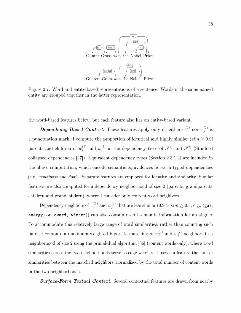
38

Günter Grass won the Nobel Prize.

nn nsubj

det

nn

dobj

Günter_Grass won the Nobel_Prize.

nsubj det

dobj

Figure 2.7: Word and entity-based representations of a sentence. Words in the same namedentity are grouped together in the latter representation.

the word-based features below, but each feature also has an entity-based variant.

Dependency-Based Context. These features apply only if neither w(1)i nor w(2)

j is

a punctuation mark. I compute the proportion of identical and highly similar (sim ≥ 0.9)

parents and children of w(1)i and w

(2)j in the dependency trees of S(1) and S(2) (Stanford

collapsed dependencies [27]). Equivalent dependency types (Section 2.3.1.2) are included in

the above computation, which encode semantic equivalences between typed dependencies

(e.g., nsubjpass and dobj ). Separate features are employed for identity and similarity. Similar

features are also computed for a dependency neighborhood of size 2 (parents, grandparents,

children and grandchildren), where I consider only content word neighbors.

Dependency neighbors of w(1)i and w(2)

j that are less similar (0.9 > sim ≥ 0.5; e.g., (gas,

energy) or (award, winner)) can also contain useful semantic information for an aligner.

To accommodate this relatively large range of word similarities, rather than counting such

pairs, I compute a maximum-weighted bipartite matching of w(1)i and w(2)

j neighbors in a

neighborhood of size 2 using the primal-dual algorithm [36] (content words only), where word

similarities across the two neighborhoods serve as edge weights. I use as a feature the sum of

similarities between the matched neighbors, normalized by the total number of content words

in the two neighborhoods.

Surface-Form Textual Context. Several contextual features are drawn from nearby

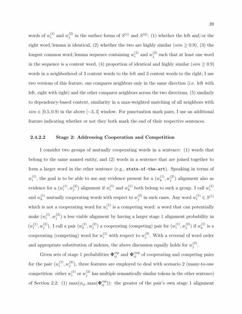
39

words of w(1)i and w(2)

j in the surface forms of S(1) and S(2): (1) whether the left and/or the

right word/lemma is identical, (2) whether the two are highly similar (sim ≥ 0.9), (3) the

longest common word/lemma sequence containing w(1)i and w(2)

j such that at least one word

in the sequence is a content word, (4) proportion of identical and highly similar (sim ≥ 0.9)

words in a neighborhood of 3 content words to the left and 3 content words to the right; I use

two versions of this feature, one compares neighbors only in the same direction (i.e. left with

left, right with right) and the other compares neighbors across the two directions, (5) similarly

to dependency-based context, similarity in a max-weighted matching of all neighbors with

sim ∈ [0.5, 0.9) in the above [−3, 3] window. For punctuation mark pairs, I use an additional

feature indicating whether or not they both mark the end of their respective sentences.

2.4.2.2 Stage 2: Addressing Cooperation and Competition

I consider two groups of mutually cooperating words in a sentence: (1) words that

belong to the same named entity, and (2) words in a sentence that are joined together to

form a larger word in the other sentence (e.g., state-of-the-art). Speaking in terms of

w(1)i , the goal is to be able to use any evidence present for a (w

(1)k , w

(2)j ) alignment also as

evidence for a (w(1)i , w

(2)j ) alignment if w(1)

i and w(1)k both belong to such a group. I call w(1)

i

and w(1)k mutually cooperating words with respect to w(2)

j in such cases. Any word w(1)l ∈ S(1)

which is not a cooperating word for w(1)i is a competing word: a word that can potentially

make (w(1)i , w

(2)j ) a less viable alignment by having a larger stage 1 alignment probability in

(w(1)l , w

(2)j ). I call a pair (w

(1)k , w

(2)j ) a cooperating (competing) pair for (w

(1)i , w

(2)j ) if w(1)

k is a

cooperating (competing) word for w(1)i with respect to w(2)

j . With a reversal of word order

and appropriate substitution of indexes, the above discussion equally holds for w(2)j .

Given sets of stage 1 probabilities Φcopij and Φcmp

ij of cooperating and competing pairs

for the pair (w(1)i , w

(2)j ), three features are employed to deal with scenario 2 (many-to-one

competition: either w(1)i or w(2)

j has multiple semantically similar tokens in the other sentence)

of Section 2.2: (1) max(φij,max(Φcopij )): the greater of the pair’s own stage 1 alignment

40

probability and the highest among all cooperating pair probabilities, (2) max(Φcmpij ): the

highest of all competing pair probabilities, and (3) a binary feature indicating which of the

two above is larger.

To address scenario 3 (many-to-many competition: both w(1)i and w(2)

j have multiple

semantically similar tokens in the other sentence), a weighted bipartite graph is constructed:

nodes represent words in S(1) and S(2) and the weight of each edge represents the stage 1

alignment probability of a word pair in S(1) × S(2). A max-weighted bipartite matching Mφ

of word pairs is identified in this graph. For each word pair, I employ a feature indicating

whether or not it is in Mφ. The presence of (w(1)i , w

(2)j ) and (w

(1)k , w

(2)l ) in Mφ, where all

four words are similar, is a potential indicator that (w(1)i , w

(2)l ) and (w

(1)k , w

(2)j ) are no longer

viable alignments.

Low recall has traditionally been the primary weakness of supervised aligners (as shown

later in Table 2.7). Observation of the aligner’s behavior on the dev set of the msr alignment

corpus [16] suggests that this happens primarily due to highly similar word pairs being

left unaligned even in the absence of competing pairs, because of relatively low contextual

evidence. Consequently, aligner performance suffers in sentences with few common or similar

words. To promote high recall, I employ the higher of a word pair’s own lexical similarity

and the lexical similarity of the cooperating pair with the highest stage 1 probability as a

stage 2 feature. This feature enables reassessment and possible alignment of semantically

similar word pairs that are otherwise left unaligned due to the above reason.

The stage 2 feature set is identical across word pair types, but as in stage 1, individual

models are trained for different pair types.

2.4.3 Experiments

I run the same experiments that were run to evaluate the unsupervised aligner in

Section 2.3. The same datasets are used for all experiments.

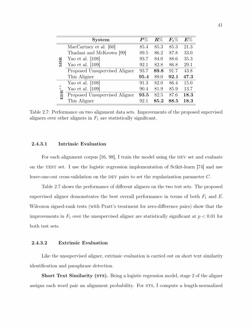
41

System P% R% F1% E%

msr

MacCartney et al. [60] 85.4 85.3 85.3 21.3Thadani and McKeown [99] 89.5 86.2 87.8 33.0Yao et al. [108] 93.7 84.0 88.6 35.3Yao et al. [109] 92.1 82.8 86.8 29.1Proposed Unsupervised Aligner 93.7 89.8 91.7 43.8This Aligner 95.4 89.0 92.1 47.3

edb

++

Yao et al. [108] 91.3 82.0 86.4 15.0Yao et al. [109] 90.4 81.9 85.9 13.7Proposed Unsupervised Aligner 93.5 82.5 87.6 18.3This Aligner 92.1 85.2 88.5 18.3

Table 2.7: Performance on two alignment data sets. Improvements of the proposed supervisedaligners over other aligners in F1 are statistically significant.

2.4.3.1 Intrinsic Evaluation

For each alignment corpus [16, 98], I train the model using the dev set and evaluate

on the test set. I use the logistic regression implementation of Scikit-learn [74] and use

leave-one-out cross-validation on the dev pairs to set the regularization parameter C.

Table 2.7 shows the performance of different aligners on the two test sets. The proposed

supervised aligner demonstrates the best overall performance in terms of both F1 and E.

Wilcoxon signed-rank tests (with Pratt’s treatment for zero-difference pairs) show that the

improvements in F1 over the unsupervised aligner are statistically significant at p < 0.01 for

both test sets.

2.4.3.2 Extrinsic Evaluation

Like the unsupervised aligner, extrinsic evaluation is carried out on short text similarity

identification and paraphrase detection.

Short Text Similarity (sts). Being a logistic regression model, stage 2 of the aligner

assigns each word pair an alignment probability. For sts, I compute a length-normalized

42

System Pearson’s r% RankHan et al. [42] 73.7 1 (original)Yao et al. [108] 46.2 66Proposed Unsupervised Aligner 67.2 7This Aligner 67.8 4

Table 2.8: Extrinsic evaluation on *SEM 2013 sts data.

sum of alignment probabilities of content word pairs across the two sentences. All pairs with

probability > 0.5 are included; the remaining pairs are included in decreasing order of their

probabilities and already included words are ignored. As before, I normalize by dividing with

the harmonic mean of the numbers of content words in the two sentences.

Table 2.8 shows the performance of different aligners on the three SemEval-2013 sts

test sets, along with the contest-winning system [42]. This aligner demonstrates a weighted

correlation of 67.8%, which is better than similar sts systems based on the other aligners.

The difference with the unsupervised aligner is statistically significant at p < 0.05 (two-sample

one-tailed z-test). Overall, it outperforms 86 of the 89 participating systems.

Paraphrase Detection. As before, a true decision is made for a test sentence pair iff

the length-normalized alignment score for the pair exceeds a threshold derived from the dev

set. Table 2.9 shows the results. Among all aligners, this supervised aligner achieves the best

F1 score and the second best accuracy.

System Accuracy% P% R% F1%

Madnani et al. [61] 77.4 79.0 89.9 84.1Yao et al. [108] 70.0 72.6 88.1 79.6Yao et al. [109] 68.1 68.6 95.8 79.9Proposed Unsupervised Aligner 73.4 76.6 86.4 81.2This Aligner 73.2 75.3 88.8 81.5

Table 2.9: Extrinsic evaluation on msr paraphrase data.

43

Model P% R% F1% E %

msr Two-Stage Model 95.4 89.0 92.1 47.3

Stage 1 Only 92.9 85.6 89.1 28.0

edb

++ Two-Stage Model 92.1 85.2 88.5 18.3

Stage 1 Only 93.0 79.0 85.4 13.7

Table 2.10: Performance with and without stage 2.

2.4.3.3 Ablation Test

I run ablation tests to find out how important (1) the two-stage framework, and (2)

the different features are for this aligner.

Results without Stage 2. Stage 1 of the aligner can operate as an aligner by itself

by mapping each alignment probability to a 0/1 alignment decision based on a threshold of

0.5. From a design perspective, this is an aligner that does not address scenarios 2 and 3 of

Section 2.2.

The performance of the aligner with and without stage 2 is shown in Table 2.10. On

each test set, the F1 and E scores increase with the addition of stage 2. On the msr test

set, performance improves along all dimensions. On the Edinburgh++ test set, the precision

drops a little, but this effect is offset by a larger improvement in recall. These results show

that stage 2 is central to the aligner’s success.

Without Different Stage 1 Features. I exclude different stage 1 features (which

fall into one of two groups: lexical and contextual) and examine the resulting model’s

performance. Table 2.11 shows the results. The subtraction sign represents the exclusion of

the corresponding feature.

Without any lexical feature (i.e., if the model relies only on contextual features), both

precision and recall decrease, resulting in a considerable overall performance drop (row 2).

Exclusion of word similarity resources (i.e. embeddings and ppdb) improves precision, but

44

msr edb++

Features P% R% F1% P% R% F1%

All Features 95.4 89.0 92.1 92.1 85.2 88.5(-) Lexical 95.1 82.8 88.5 90.9 84.0 87.3(-) Resources 96.0 87.0 91.3 92.2 84.3 88.1(-) Contextual 89.0 79.2 83.9 89.9 66.3 76.3(-) Dependency 95.3 88.2 91.6 91.9 84.9 88.3(-) Surface 94.4 85.6 89.8 90.6 76.9 83.2(-) Word-Based 94.6 87.7 91.0 92.0 85.1 88.4(-) Entity-Based 95.5 89.0 92.1 92.1 85.1 88.5

Table 2.11: Results without different stage 1 features.

again harms overall performance (row 3).

Without any contextual features, the model suffers badly in both precision and recall

(row 4). The extreme overall performance degradation indicates that contextual features are

more important for the aligner than lexical features. Leaving out surface-form neighbors

results in a larger performance drop than when dependency-based neighbors are excluded,

pointing to a more robust role of the former group in representing context (rows 5 and 6).

Finally, the entity-based representation of context neither helps nor harms system performance

(row 8), but relying only on entity-based neighbors has detrimental effects (row 7). Factoring

in semantic similarities of named entities should improve the utility of these features.

Without Different Stage 2 Features. Table 2.12 shows the aligner’s performance

after the exclusion of different stage 2 features. Leaving out the stage 1 alignment probabilities

msr edb++

Features P% R% F1% P% R% F1%All Features 95.4 89.0 92.1 92.1 85.2 88.5(-) φ values 87.3 90.7 88.9 86.4 86.9 86.7(-) Matching 95.3 87.9 91.5 92.3 84.6 88.3(-) Word Sim 95.5 88.4 91.8 92.7 84.7 88.5

Table 2.12: Results without different stage 2 features.

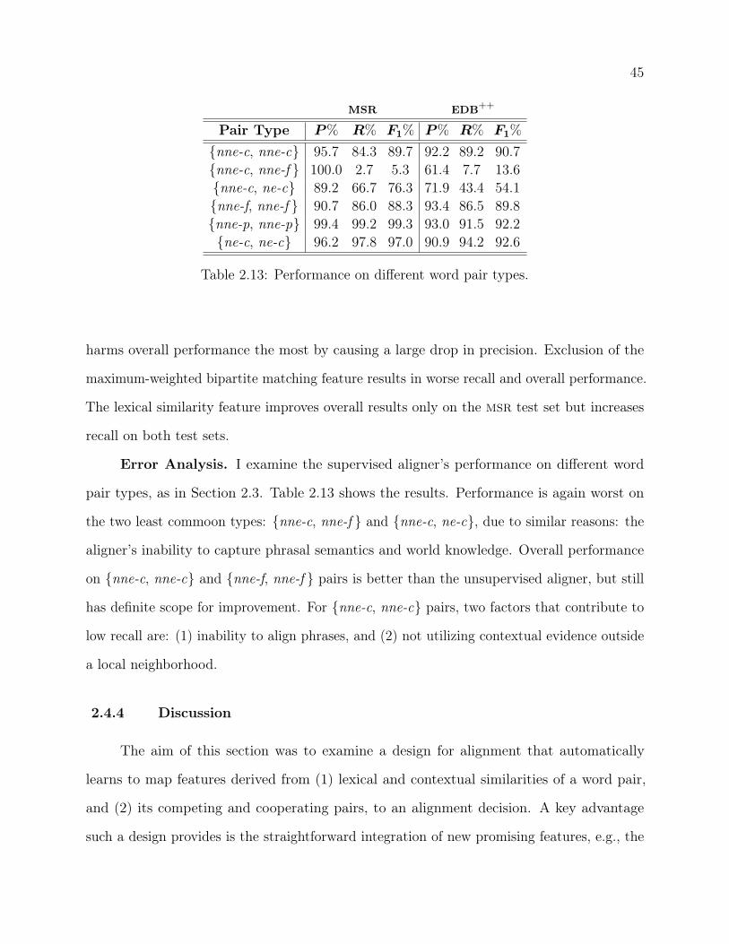
45

msr edb++

Pair Type P% R% F1% P% R% F1%{nne-c, nne-c} 95.7 84.3 89.7 92.2 89.2 90.7{nne-c, nne-f } 100.0 2.7 5.3 61.4 7.7 13.6{nne-c, ne-c} 89.2 66.7 76.3 71.9 43.4 54.1{nne-f, nne-f } 90.7 86.0 88.3 93.4 86.5 89.8{nne-p, nne-p} 99.4 99.2 99.3 93.0 91.5 92.2{ne-c, ne-c} 96.2 97.8 97.0 90.9 94.2 92.6

Table 2.13: Performance on different word pair types.

harms overall performance the most by causing a large drop in precision. Exclusion of the

maximum-weighted bipartite matching feature results in worse recall and overall performance.

The lexical similarity feature improves overall results only on the msr test set but increases

recall on both test sets.

Error Analysis. I examine the supervised aligner’s performance on different word

pair types, as in Section 2.3. Table 2.13 shows the results. Performance is again worst on

the two least commoon types: {nne-c, nne-f } and {nne-c, ne-c}, due to similar reasons: the

aligner’s inability to capture phrasal semantics and world knowledge. Overall performance

on {nne-c, nne-c} and {nne-f, nne-f } pairs is better than the unsupervised aligner, but still

has definite scope for improvement. For {nne-c, nne-c} pairs, two factors that contribute to

low recall are: (1) inability to align phrases, and (2) not utilizing contextual evidence outside

a local neighborhood.

2.4.4 Discussion

The aim of this section was to examine a design for alignment that automatically

learns to map features derived from (1) lexical and contextual similarities of a word pair,

and (2) its competing and cooperating pairs, to an alignment decision. A key advantage

such a design provides is the straightforward integration of new promising features, e.g., the

46

lexical similarity measure using neural word embeddings. Based on similar design elements,

this model outperforms the unsupervised model of Section 2.3. A major drawback of the

model is its relatively complicated design, leading also to a higher runtime. It also shares

the limitations with the unsupervised aligner of not aligning phrases and utilizing only local

information for context representation.

2.5 Conclusions

In view of the importance of alignment for sts, this chapter presents two monolingual

word aligners. Both aligners demonstrate top results in intrinsic evaluation. Primary results

also indicate that they are promising for sts. Of the two, the unsupervised aligner has

the advantages of speed and ease of implementation, with only marginally worse overall

performance. The following chapters discuss its use as a major system component in two

novel sts systems and their real-life applications.

Chapter 3

Algorithms for Short-Text Semantic Similarity

This chapter explores the central research problem of this dissertation: design of

algorithms for short text similarity (sts). In view of sts as a high-utility task, I seek to

develop algorithms that are effective, efficient, and easily replicable. In later chapters, I also

explore their utility in the context of question answering and short answer grading.

The unsupervised aligner of Chapter 2 plays a central role in the sts algorithms

presented in this chapter. Extrinsic evaluation of the aligner on sts indicated that an

effective sts algorithm can be developed based solely on alignment. I first explore this

idea in depth (Section 3.4); alignment is then used as a feature in a supervised sts model

(Section 3.5). These algorithms [89, 91] were the winners at the SemEval Semantic Textual

Similarity task in 2014 and 2015, respectively [1, 2].

In the context of this dissertation, studies reported in this chapter are designed to

answer RQ2 of Section 1.3: How can sts algorithms be designed using alignment

of related concepts in the two input snippets? I describe the proposed algorithms

following an introductory discussion of sts and related prior work.

3.1 Short-Text Semantic Similarity

Given short text snippets S(1) = (w(1)1 , ..., w

(1)n ) and S(2) = (w

(2)1 , ..., w

(2)m ), where each w

is a word token, the goal of sts is to compute a bounded real-valued score sim(S(1), S(2)) that

represents the degree of semantic similarity between S(1) and S(2). Table 3.1 shows examples

48

Sentence 1 Sentence 2 Similarity

The bird is bathing in the sink. Birdie is washing itself in the waterbasin. 5.0

In May 2010, the troops attemptedto invade Kabul.

The US army invaded Kabul on May7th last year, 2010. 4.0

John said he is considered a witnessbut not a suspect.

“He is not a suspect anymore.” Johnsaid. 3.0

They flew out of the nest in groups. They flew into the nest together. 2.0

The woman is playing the violin. The young lady enjoys listening tothe guitar. 1.0

John went horse back riding at dawnwith a whole group of friends.

Sunrise at dawn is a magnificent viewto take in if you wake up early enoughfor it.

0.0

Table 3.1: Human-assigned similarity scores to pairs of sentences on a 0–5 scale. Examplesare taken from [1]. Interpretation of each similarity level is shown in Table 3.2.

of sentence pairs that received various similarity scores on a 0–5 scale from human judges

at the SemEval Semantic Textual Similarity task [1, 2, 3, 4]. Like most natural language

processing tasks, such human-assigned scores serve as the gold standard for sts—the goal of

an algorithm is to output scores that are close to human annotations.

At SemEval, annotators provide these scores on a Likert scale. Organizers define the

levels beforehand, as shown in Table 3.2. Averaging over multiple human annotations results

in a real-valued score for each pair. Algorithms also output real-valued scores; the Pearson

product-moment correlation coefficient (Pearson’s r) of these scores with average human

annotations is used for evaluation. Evaluation is explained in more detail later in this chapter.

It is important to note the difference between sts and two other text comparison

tasks: paraphrase detection and textual entailment recognition. In paraphrase detection, the

output is a binary variable indicating whether or not the meanings of two input sentences

are the same [30, 61, 86]. Thus it effectively merges all the levels below 5.0 in Table 3.2 to a

single non-paraphrase class label. In textual entailment recognition [23, 39], the output is

again a binary variable, but one that indicates whether the truth value of one sentence—the

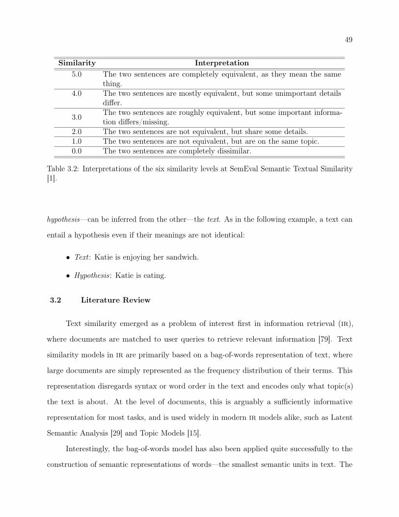
49

Similarity Interpretation5.0 The two sentences are completely equivalent, as they mean the same

thing.4.0 The two sentences are mostly equivalent, but some unimportant details

differ.

3.0 The two sentences are roughly equivalent, but some important informa-tion differs/missing.

2.0 The two sentences are not equivalent, but share some details.1.0 The two sentences are not equivalent, but are on the same topic.0.0 The two sentences are completely dissimilar.

Table 3.2: Interpretations of the six similarity levels at SemEval Semantic Textual Similarity[1].

hypothesis—can be inferred from the other—the text. As in the following example, a text can

entail a hypothesis even if their meanings are not identical:

• Text : Katie is enjoying her sandwich.

• Hypothesis : Katie is eating.

3.2 Literature Review

Text similarity emerged as a problem of interest first in information retrieval (ir),

where documents are matched to user queries to retrieve relevant information [79]. Text

similarity models in ir are primarily based on a bag-of-words representation of text, where

large documents are simply represented as the frequency distribution of their terms. This

representation disregards syntax or word order in the text and encodes only what topic(s)

the text is about. At the level of documents, this is arguably a sufficiently informative

representation for most tasks, and is used widely in modern ir models alike, such as Latent

Semantic Analysis [29] and Topic Models [15].

Interestingly, the bag-of-words model has also been applied quite successfully to the

construction of semantic representations of words—the smallest semantic units in text. The

50

basic idea is to represent a word’s meaning as a direct function of the context in which

it appears across a large number of documents. Context of a token t in a given piece of

text is defined as the set of tokens surrounding t within a pre-specified window size. Such

distributional models represent a target word as a point in a vector space, derived from raw

frequencies of its neighboring words or transformations such as dimensionality reduction

applied to these frequencies [20, 32]. The latest generation of distributional models learn

word vectors (also known as word embeddings) that maximize the probability of observing

each target word in its contexts in a large corpus [10, 12, 22, 65]. These word representations

provide a much greater coverage than manually constructed lexical resources like WordNet

[66] and have demonstrated excellent results in identification of word similarity [10]. Other

approaches to identifying lexically similar words include bilingual pivoting (ppdb [37]) and

combination of distributional and resource-based measures [41].

Semantics of short snippets such as sentences, however, is not effectively captured in a

bag-of-words representation. Unlike documents, a sentence’s meaning is a function of not

only what words it contains, but also their position in the sentence and the complex semantic

relationships that emerge from it. Unlike words, sentences are not observed frequently enough

even in the largest of corpora for the context-based model to be useful in practice.

Early work in sentence similarity [48, 56, 64] identifies the key requirements of (1)

finding semantically similar or related word pairs across the two input sentences, and (2)

incorporating some measure of syntactic similarity between the sentences. Sentence similarity

is then computed as a function (such as a weighted sum) of these measures. Both resource-

based (e.g., WordNet) and distributional (e.g., pointwise mutual information) measures are

employed for word similarity, while word order is used as a simplistic representation of syntax.

In recent times, the majority of work in short text similarity has been done at the

SemEval Semantic Textual Similarity task [1, 2, 3, 4]. A key outcome of the series is a dataset

of over 14, 000 human-annotated sentence pairs, which I discuss in the next section. Another

major outcome is a rich literature for sts, describing around 300 sts systems that have been

51

evaluated over a span of 4 years (2012–2015). A vast majority of the best-performing systems

at SemEval apply a regression algorithm that predicts similarity as a linear function of a

wide array of text similarity measures [6, 8, 43, 59, 62, 84, 101, 105]. Common feature groups

include (1) shallow string similarity measures such as the longest common subsequence, word

and character n-gram overlap, (2) semantic similarity measures derived from lexical similarity

resources (such as WordNet) and distributional measures (such as latent semantic analysis

(lsa) [29]), (3) syntactic measures such as dependency overlap, and (4) output of previous

top-performing systems such as the ones described in [8, 42, 101]. Even though this design is

highly effective in general, it performs the best when in-domain training data with properties

very similar to the test dataset is available. Without such training data at SemEval 2013–2015,

these systems are outperformed by (1) unsupervised systems that align semantically related

words in the two sentences [42, 89], and (2) supervised systems with fewer features [91].1

Surprisingly, a set of systems based primarily on character n-gram overlap are among the

top-performing systems across test datasets from different years [49, 50, 59].

Other interesting ideas that have been explored in the context of sts include domain

adaptation [38, 45], application of tree kernels [83] and probabilistic soft logic [11], and

development of algorithms that can adapt to texts of different length (e.g., words, sentences,

and documents) [75]. sts algorithms have also been developed for extrinsic tasks such as

answer sentence ranking for factoid question answering [82, 107, 113], short answer grading

[68, 77], text reuse detection [9, 21], and identification of core domain concepts in educational

resources [90]. Finally, systems developed for related tasks such as paraphrase detection

[24, 30, 61, 86] and textual entailment recognition [23, 39] can also inform the design of new

sts systems.

1These high-performing systems at SemEval 2013–2015 include the two systems proposed in Sections 3.4

and 3.5 of this chapter [89, 91].

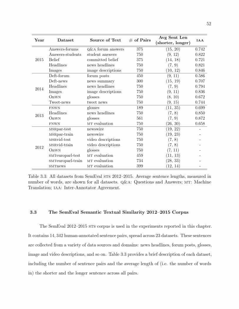
52

Year Dataset Source of Text # of Pairs Avg Sent Len iaa(shorter, longer)

2015

Answers-forums q&a forum answers 375 (15, 20) 0.742Answers-students student answers 750 (9, 12) 0.822Belief committed belief 375 (14, 18) 0.721Headlines news headlines 750 (7, 9) 0.821Images image descriptions 750 (10, 12) 0.846

2014

Deft-forum forum posts 450 (9, 11) 0.586Deft-news news summary 300 (15, 19) 0.707Headlines news headlines 750 (7, 9) 0.794Images image descriptions 750 (9, 11) 0.836Onwn glosses 750 (8, 10) 0.672Tweet-news tweet news 750 (9, 15) 0.744

2013

fnwn glosses 189 (11, 35) 0.699Headlines news headlines 750 (7, 8) 0.850Onwn glosses 561 (7, 9) 0.872fnwn mt evaluation 750 (26, 30) 0.658

2012

msrpar-test newswire 750 (19, 22) -msrpar-train newswire 750 (19, 23) -msrvid-test video descriptions 750 (7, 8) -msrvid-train video descriptions 750 (7, 8) -Onwn glosses 750 (7, 11) -smteuroparl-test mt evaluation 459 (11, 13) -smteuroparl-train mt evaluation 734 (28, 33) -smtnews mt evaluation 399 (12, 14) -

Table 3.3: All datasets from SemEval sts 2012–2015. Average sentence lengths, measured innumber of words, are shown for all datasets. q&a: Questions and Answers; mt: MachineTranslation; iaa: Inter-Annotator Agreement.

3.3 The SemEval Semantic Textual Similarity 2012–2015 Corpus

The SemEval 2012–2015 sts corpus is used in the experiments reported in this chapter.

It contains 14, 342 human-annotated sentence pairs, spread across 23 datasets. These sentences

are collected from a variety of data sources and domains: news headlines, forum posts, glosses,

image and video descriptions, and so on. Table 3.3 provides a brief description of each dataset,

including the number of sentence pairs and the average length of (i.e. the number of words

in) the shorter and the longer sentence across all pairs.

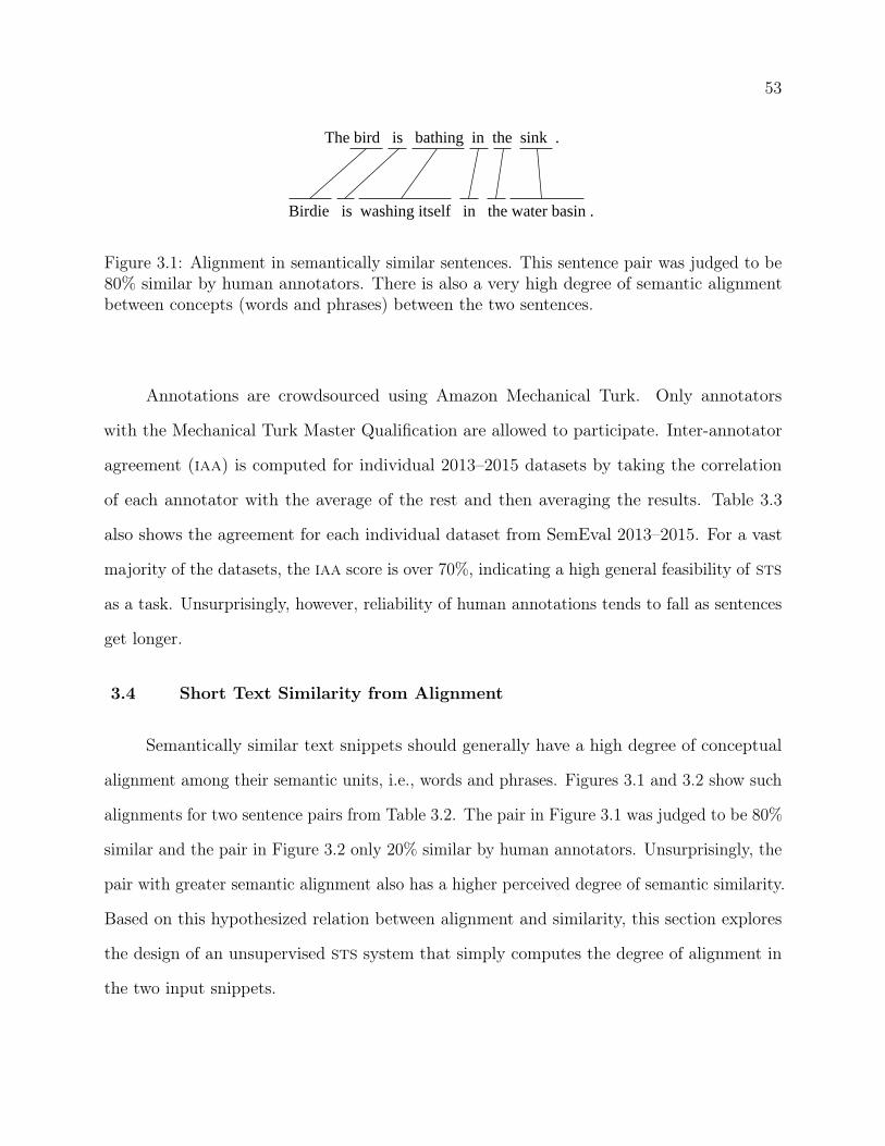
53

The bird is bathing in the sink .

Birdie is washing itself in the water basin .

Figure 3.1: Alignment in semantically similar sentences. This sentence pair was judged to be80% similar by human annotators. There is also a very high degree of semantic alignmentbetween concepts (words and phrases) between the two sentences.

Annotations are crowdsourced using Amazon Mechanical Turk. Only annotators

with the Mechanical Turk Master Qualification are allowed to participate. Inter-annotator

agreement (iaa) is computed for individual 2013–2015 datasets by taking the correlation

of each annotator with the average of the rest and then averaging the results. Table 3.3

also shows the agreement for each individual dataset from SemEval 2013–2015. For a vast

majority of the datasets, the iaa score is over 70%, indicating a high general feasibility of sts

as a task. Unsurprisingly, however, reliability of human annotations tends to fall as sentences

get longer.

3.4 Short Text Similarity from Alignment

Semantically similar text snippets should generally have a high degree of conceptual

alignment among their semantic units, i.e., words and phrases. Figures 3.1 and 3.2 show such

alignments for two sentence pairs from Table 3.2. The pair in Figure 3.1 was judged to be 80%

similar and the pair in Figure 3.2 only 20% similar by human annotators. Unsurprisingly, the

pair with greater semantic alignment also has a higher perceived degree of semantic similarity.

Based on this hypothesized relation between alignment and similarity, this section explores

the design of an unsupervised sts system that simply computes the degree of alignment in

the two input snippets.

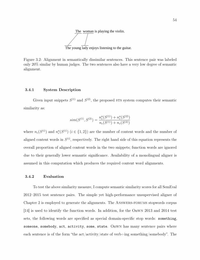
54

The woman is playing the violin.

The young lady enjoys listening to the guitar.

Figure 3.2: Alignment in semantically dissimilar sentences. This sentence pair was labeledonly 20% similar by human judges. The two sentences also have a very low degree of semanticalignment.

3.4.1 System Description

Given input snippets S(1) and S(2), the proposed sts system computes their semantic

similarity as:

sim(S(1), S(2)) =nac(S

(1)) + nac(S(2))

nc(S(1)) + nc(S(2))

where nc(S(i)) and nac(S(i)) (i ∈ {1, 2}) are the number of content words and the number of

aligned content words in S(i), respectively. The right hand side of this equation represents the

overall proportion of aligned content words in the two snippets; function words are ignored

due to their generally lower semantic significance. Availability of a monolingual aligner is

assumed in this computation which produces the required content word alignments.

3.4.2 Evaluation

To test the above similarity measure, I compute semantic similarity scores for all SemEval

2012–2015 test sentence pairs. The simple yet high-performance unsupervised aligner of

Chapter 2 is employed to generate the alignments. The Answers-forums stopwords corpus

[14] is used to identify the function words. In addition, for the Onwn 2013 and 2014 test

sets, the following words are specified as special domain-specific stop words: something,

someone, somebody, act, activity, some, state. Onwn has many sentence pairs where

each sentence is of the form “the act/activity/state of verb+ing something/somebody”. The

55

above words act merely as fillers in such pairs and consequently do not typically contribute

to the similarity scores.

Table 3.4 shows the performance of the system alongside the inter-annotator agreement

(iaa) and performances of the following:

• Token-Cos: A word overlap baseline that represents each sentence as a one-hot vector.

Each element of the vector corresponds to a token from either of the two sentences

and is 1 iff the token is present in the sentence. The cosine similarity between the

two sentence vectors is output as their similarity score.

• The winning system at SemEval for that year. The top-performing system in 2014

[89] is a variation of the system proposed in this section—the two systems are based

on the same unsupervised aligner, but employ two slightly different formulas to derive

similarity from alignment. In 2015, the system discussed in the next section performed

the best [91]. The winning system in 2013 [42] also employs an unsupervised algorithm

based on alignment, with one important difference with the system proposed here:

their alignment algorithm uses no measure of contextual similarity. The two systems

also differ significantly in the lexical resources they employ (ppdb versus WordNet

and lsa). Finally, the winning system at SemEval-2012 [8] uses various independently

computed measures of similarity (e.g., surface-form, syntactic, and semantic) within

a regression model.

Following SemEval, Pearson’s r with human annotations is first computed for each

individual test set. For each year, results from all test sets are then combined by taking a

weighted sum—the weight of a test set is proportional to its number of sentence pairs.

The simple similarity equation of Section 3.4.1 performs surprisingly well across test

sets from different SemEval years. On 2014 and 2015 data, its performance is comparable to

that of human annotators. On 2013 and 2014 data, it demonstrates better overall results than

the winning systems. Over all the other systems, it also has the two following key advantages:

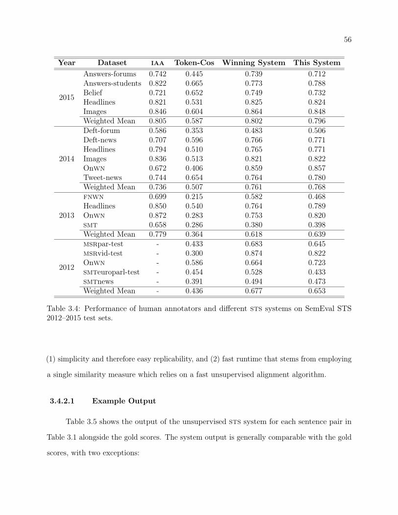
56

Year Dataset iaa Token-Cos Winning System This System

2015

Answers-forums 0.742 0.445 0.739 0.712Answers-students 0.822 0.665 0.773 0.788Belief 0.721 0.652 0.749 0.732Headlines 0.821 0.531 0.825 0.824Images 0.846 0.604 0.864 0.848Weighted Mean 0.805 0.587 0.802 0.796

2014

Deft-forum 0.586 0.353 0.483 0.506Deft-news 0.707 0.596 0.766 0.771Headlines 0.794 0.510 0.765 0.771Images 0.836 0.513 0.821 0.822Onwn 0.672 0.406 0.859 0.857Tweet-news 0.744 0.654 0.764 0.780Weighted Mean 0.736 0.507 0.761 0.768

2013

fnwn 0.699 0.215 0.582 0.468Headlines 0.850 0.540 0.764 0.789Onwn 0.872 0.283 0.753 0.820smt 0.658 0.286 0.380 0.398Weighted Mean 0.779 0.364 0.618 0.639

2012

msrpar-test - 0.433 0.683 0.645msrvid-test - 0.300 0.874 0.822Onwn - 0.586 0.664 0.723smteuroparl-test - 0.454 0.528 0.433smtnews - 0.391 0.494 0.473Weighted Mean - 0.436 0.677 0.653

Table 3.4: Performance of human annotators and different sts systems on SemEval STS2012–2015 test sets.

(1) simplicity and therefore easy replicability, and (2) fast runtime that stems from employing

a single similarity measure which relies on a fast unsupervised alignment algorithm.

3.4.2.1 Example Output

Table 3.5 shows the output of the unsupervised sts system for each sentence pair in

Table 3.1 alongside the gold scores. The system output is generally comparable with the gold

scores, with two exceptions:

57

Sentence 1 Sentence 2 Gold Output

The bird is bathing in the sink. Birdie is washing itself in the waterbasin. 5.0 1.4

In May 2010, the troops attempted toinvade Kabul.

The US army invaded Kabul on May7th last year, 2010. 4.0 3.3

John said he is considered a witnessbut not a suspect.

“He is not a suspect anymore.” Johnsaid. 3.0 3.3

They flew out of the nest in groups. They flew into the nest together. 2.0 3.3

The woman is playing the violin. The young lady enjoys listening to theguitar. 1.0 1.3

John went horse back riding at dawnwith a whole group of friends.

Sunrise at dawn is a magnificent viewto take in if you wake up early enoughfor it.

0.0 0.6

Table 3.5: Examples of sentence similarity scores computed by the unsupervised sts algorithm.

(1) For the pair with gold score 5.0, the system score is very low. A closer examination

shows that the aligner only aligns bird with birdie and fails to detect the other

alignments (as shown in Figure 3.1). For the pair (bathing, washing), this happens

due to an incorrect lemmatization of bathing to itself, instead of bath or bathe.

While both (bath, wash) and (bathe, wash) are in ppdb, (bathing, wash) is

not. Similarly, the pair (sink, basin) is not in ppdb, even though a similar pair

(sink, washbasin) is. Augmenting ppdb with all possible surface forms of all words

and using additional lexical resources can help to alleviate these problems.

(2) The system outputs a high score for the pair with gold score 2.0. This is a much

more difficult scenario where the sentence pair has a low perceived semantic similarity

despite high similarity at the lexical level. This is caused solely by the difference

between flew out of and flew into. Correct assessment of such pairs will require

both incorporation of phrasal semantics and learning how semantic properties such

as polarity influence human judgment of similarity.

58

3.4.2.2 Limitations and Error Analysis

While the simple alignment-based design of the proposed system relying on a small

number of external resources reduces error propagation and improves efficiency, certain useful

predictors are left unutilized. The above examples demonstrate two key limitations. Related

words that are not paraphrases (e.g., temperature and hot) are another source of potentially

useful but unutilized information. Long-distance semantic relationships within sentences are

not effectively captured by the system. Stop words can encode important aspects of semantics

such as tense, polarity, and modality, which are ignored by the system. World knowledge is

required to recognize the semantic similarity between sentence pairs such as “Thank you very

much!” and “You’re the best!”, which is also beyond the capabilities of the system. Finally, it

is not clear how well the alignment-based algorithm approximates the process that underlies

human judgment of short text similarity.

Experimental results reported in Table 3.4 show two scenarios where the system’s

performance is relatively poor. First, performance on machine translation pairs is constantly

and considerably worse than on other sources of text. This is true of sts systems in general—

consider the winning systems in 2012 and 2013, for instance. A closer examination shows

that similarity annotations in machine translation test sets have a much smaller variance

than other test sets. Correlation in such cases can be a difficult metric to maximize, as tiny

differences between system output and gold scores can cause a large drop in accuracy. Second,

when in-domain training data is available (e.g., on the 2012 test sets msrpar-test, msrvid-test,

and smteuroparl-test), supervised systems such as the winning system at SemEval-2012

outperform the proposed system.

3.5 A Supervised sts Model

This section presents a supervised sts model designed to address some of the limitations

of the proposed unsupervised system. Specifically, it (1) uses word embeddings to represent

59

the semantic relatedness between non-paraphrase words, and (2) enables data-driven model

supervision, which can be helpful when in-domain human annotations of text similarity are

available.

3.5.1 System Description

The proposed system trains a ridge regression model (linear regression with L2 regular-

ization and error) with two different measures of text similarity as features:

• Alignment-based similarity: Output of the unsupervised sts system of Sec-

tion 3.4, as given by the equation in Section 3.4.1.

• Similarity between sentence vectors: A vector representation of each input

snippet is first constructed by simply adding its content lemma embeddings. The

400-dimensional word embeddings developed by Baroni et al. [10] are used. These

embeddings are developed using the word2vec toolkit2 from a corpus of about 2.8

billion tokens, using the Continuous Bag-of-Words (cbow) model proposed by

Mikolov et al. [65]. Given the sentence vectors, their cosine similarity is used as the

second similarity feature for the supervised sts system.

Trained on all annotated sentence pairs from SemEval 2012–2015, the model learns the

following parameter values:

• Intercept = -0.0025,

• Weight of alignment-based similarity = 0.6393,

• Weight of vector-based similarity = 0.3291.

2https://code.google.com/p/word2vec/

60

Domain of Text Datasets

Forum posts Answers-forums (2015)Deft-forum (2014)

Student answers Answers-students (2015)Committed belief Belief (2015)

News

Headlines (2015, 2014, 2013)Deft-news (2014)Tweet-news (2014)msrpar-train (2012), msrpar-test (2012)

Image and video descriptions Images (2015, 2014)msrvid-train (2012), msrvid-test (2012)

Glosses Onwn (2014, 2013, 2012)fnwn (2013)

Machine translationsmt (2013)smtnews (2012)smteuroparl-train (2012), smteuroparl-test (2012)

Table 3.6: Different source domains of text at SemEval sts 2012–2015.

3.5.2 Evaluation

The setup of Section 3.4.2 is replicated to evaluate the supervised sts model. For each

test set, I employ two different models: (1) a model trained on all annotations from all past

SemEval datasets, and (2) a second model trained on all in-domain annotations from past

years. For the latter, the datasets are grouped into different domains as shown in Table 3.6

based on their source of text (discussed in Table 3.3). For any test set that does not have an

in-domain training set available, all past SemEval data are used for training.

Table 3.7 shows the results. The last two columns show the performance of the

supervised model trained on the two different types of training data.3 Trained on in-domain

data, the model outperforms all SemEval winning systems from all years. This is a remarkable

result given the simplicity of the system. Similar performances are observed with all available

3Note that this is the winning system at SemEval-2015; the results reported here are observed after a few

minor bug fixes.

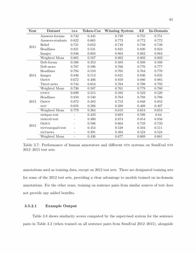
61

Year Dataset iaa Token-Cos Winning System All In-Domain

2015

Answers-forums 0.742 0.445 0.739 0.755 0.751Answers-students 0.822 0.665 0.773 0.772 0.772Belief 0.721 0.652 0.749 0.749 0.749Headlines 0.821 0.531 0.825 0.820 0.824Images 0.846 0.604 0.864 0.862 0.864Weighted Mean 0.805 0.587 0.802 0.802 0.803

2014

Deft-forum 0.586 0.353 0.483 0.508 0.508Deft-news 0.707 0.596 0.766 0.776 0.777Headlines 0.794 0.510 0.765 0.764 0.770Images 0.836 0.513 0.821 0.836 0.835Onwn 0.672 0.406 0.859 0.880 0.885Tweet-news 0.744 0.654 0.764 0.798 0.792Weighted Mean 0.736 0.507 0.761 0.779 0.780

2013

fnwn 0.699 0.215 0.582 0.523 0.528Headlines 0.850 0.540 0.764 0.788 0.786Onwn 0.872 0.283 0.753 0.848 0.852smt 0.658 0.286 0.380 0.408 0.407Weighted Mean 0.779 0.364 0.618 0.654 0.654

2012

msrpar-test - 0.433 0.683 0.598 0.64msrvid-test - 0.300 0.874 0.854 0.856Onwn - 0.586 0.664 0.733 0.733smteuroparl-test - 0.454 0.528 0.504 0.511smtnews - 0.391 0.494 0.524 0.524Weighted Mean - 0.436 0.677 0.669 0.681

Table 3.7: Performance of human annotators and different sts systems on SemEval sts2012–2015 test sets.

annotations used as training data, except on 2012 test sets. There are designated training sets

for some of the 2012 test sets, providing a clear advantage to models trained on in-domain

annotations. For the other years, training on sentence pairs from similar sources of text does

not provide any added benefits.

3.5.2.1 Example Output

Table 3.8 shows similarity scores computed by the supervised system for the sentence

pairs in Table 3.2 (when trained on all sentence pairs from SemEval 2012–2015), alongside

62

Sentence 1 Sentence 2 G S A E

The bird is bathing in the sink. Birdie is washing itself in the wa-ter basin. 5.0 1.8 1.4 2.6

In May 2010, the troops at-tempted to invade Kabul.

The US army invaded Kabul onMay 7th last year, 2010. 4.0 3.5 3.3 4.1

John said he is considered a wit-ness but not a suspect.

“He is not a suspect anymore.”John said. 3.0 3.4 3.3 3.8

They flew out of the nest ingroups.

They flew into the nest together. 2.0 3.6 3.3 4.5

The woman is playing the violin. The young lady enjoys listeningto the guitar. 1.0 1.7 1.3 2.7

John went horse back riding atdawn with a whole group offriends.

Sunrise at dawn is a magnificentview to take in if you wake upearly enough for it.

0.0 1.2 0.6 2.7

Table 3.8: Examples of sentence similarity scores computed by the supervised system. G:gold score, S: supervised sts system score, A: the alignment-based similarity score, E: cosinesimilarity between sentence embeddings.

human annotations. I also show similarity scores based on alignment and sentence vectors.

Scores computed by the supervised system are generally higher than those computed by the

unsupervised system (i.e. the alignment-based similarity scores), because of higher embedding-

based similarity values. Overall, however, the pattern is similar to the unsupervised system

on this set of examples, with the model doing well except on the pairs with gold scores 5.0

and 2.0.

3.5.2.2 Ablation Study

To assess the two individual features of the system, I run an ablation study on all

SemEval test sets. Table 3.9 shows the performance of the system (in-domain training)

alongside that of each feature. Overall, alignment-based similarity is the more useful of

the two features. Importantly, however, addition of the embedding-based feature improves

performance on almost all test sets. This includes machine translation pairs, on which the

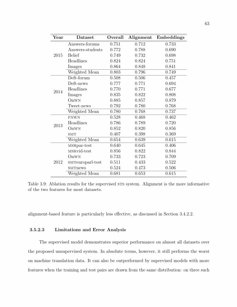
63

Year Dataset Overall Alignment Embeddings

2015

Answers-forums 0.751 0.712 0.733Answers-students 0.772 0.788 0.690Belief 0.749 0.732 0.698Headlines 0.824 0.824 0.751Images 0.864 0.848 0.841Weighted Mean 0.803 0.796 0.749

2014

Deft-forum 0.508 0.506 0.457Deft-news 0.777 0.771 0.694Headlines 0.770 0.771 0.677Images 0.835 0.822 0.808Onwn 0.885 0.857 0.879Tweet-news 0.792 0.780 0.768Weighted Mean 0.780 0.768 0.737

2013

fnwn 0.528 0.468 0.462Headlines 0.786 0.789 0.720Onwn 0.852 0.820 0.856smt 0.407 0.398 0.369Weighted Mean 0.654 0.639 0.615

2012

msrpar-test 0.640 0.645 0.406msrvid-test 0.856 0.822 0.844Onwn 0.733 0.723 0.709smteuroparl-test 0.511 0.433 0.522smtnews 0.524 0.473 0.506Weighted Mean 0.681 0.653 0.615

Table 3.9: Ablation results for the supervised sts system. Alignment is the more informativeof the two features for most datasets.

alignment-based feature is particularly less effective, as discussed in Section 3.4.2.2.

3.5.2.3 Limitations and Error Analysis

The supervised model demonstrates superior performance on almost all datasets over

the proposed unsupervised system. In absolute terms, however, it still performs the worst

on machine translation data. It can also be outperformed by supervised models with more

features when the training and test pairs are drawn from the same distribution: on three such

64

test sets from SemEval-2012 (msrpar-test, msrvid-test, and smteuroparl-test), the winning

system [8] shows better correlation with human annotators than the proposed model. This is

arguably a less common scenario in practice, however, which can be addressed by adding

additional measures of similarity (e.g., word and character n-gram overlap, and more lexical

similarity measures) as features to the existing model. The difficult challenges posed by stop

word semantics and world knowledge (discussed in Section 3.4.2.2) also remain unaddressed

by this model.

3.6 Conclusions and Future Work

This chapter presents two algorithms for short text similarity. The simpler unsupervised

algorithm aligns semantically similar words and named entities in the two input snippets based

on their lexical and contextual similarity. The proportion of aligned content words in the two

snippets serves as a measure of their semantic similarity. To address some of its limitations,

this system is then augmented with an additional measure of semantic similarity within a

regression model. This measure is derived from an unsupervised composition of pre-computed

word embeddings in the two sentences. This supervised model shows outstanding performance

on SemEval 2012–2015 data—the benchmark dataset for virtually all recent work in sts—by

maintaining the best correlation with human annotators among all sts systems to date.

In addition to high performance, a simple design with straightforward implementation

makes the proposed systems potentially extremely useful in the context of various sts

applications. In the following chapters, I explore the utility of the supervised model in two

such tasks: question answering and short answer grading.

sts offers immense scope for future research, some of which have been mentioned in

the discussions of the proposed models’ limitations. Effective representation of (1) phrasal

semantics, (2) subtleties encoded in stop words, and (3) world knowledge are among the

biggest open problems in nlp, solutions to which can produce key design elements for future

sts systems.

Chapter 4

Short Text Similarity for Automatic Question Answering

One of the original goals of AI was to build machines that can naturally interact with

humans. Over time, the challenges became apparent and language processing emerged as

one of ai’s most puzzling areas. Nevertheless, major breakthroughs have still been made in

several important nlp tasks; with the astounding performance of ibm’s Watson [33] in the

quiz contest Jeopardy!, question answering (qa) is definitely one such task.

Question answering comes in various forms, each supporting specific kinds of user

requirements. Consider a scenario where a system is given a question and a set of sentences

each of which may or may not contain an answer to that question. The goal of Answer

Extraction is to extract a precise answer in the form of a short span of text in one or more

of those sentences. In this form, qa meets users’ immediate information needs. Answer

Sentence Ranking, on the other hand, is the task of assigning a rank to each sentence

so that the ones that contain an answer are ranked higher. In this form, qa is similar to

information retrieval and presents greater opportunities for further exploration and learning.

This chapter proposes a novel approach to jointly solving these two well-studied yet open

qa problems, where the supervised short text similarity (sts) model of Chapter 3 is a key

system component.

Most existing answer sentence ranking algorithms operate under the assumption that

the degree of syntactic and/or semantic similarity between questions and answer sentences

is a sufficiently strong predictor of answer sentence relevance [82, 104, 111, 113]. On the

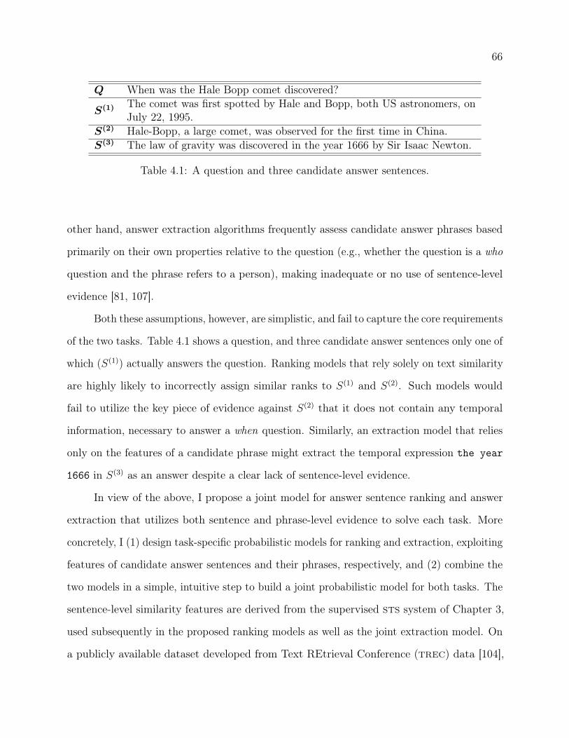
66

Q When was the Hale Bopp comet discovered?

S(1) The comet was first spotted by Hale and Bopp, both US astronomers, onJuly 22, 1995.

S(2) Hale-Bopp, a large comet, was observed for the first time in China.S(3) The law of gravity was discovered in the year 1666 by Sir Isaac Newton.

Table 4.1: A question and three candidate answer sentences.

other hand, answer extraction algorithms frequently assess candidate answer phrases based

primarily on their own properties relative to the question (e.g., whether the question is a who

question and the phrase refers to a person), making inadequate or no use of sentence-level

evidence [81, 107].

Both these assumptions, however, are simplistic, and fail to capture the core requirements

of the two tasks. Table 4.1 shows a question, and three candidate answer sentences only one of

which (S(1)) actually answers the question. Ranking models that rely solely on text similarity

are highly likely to incorrectly assign similar ranks to S(1) and S(2). Such models would

fail to utilize the key piece of evidence against S(2) that it does not contain any temporal

information, necessary to answer a when question. Similarly, an extraction model that relies

only on the features of a candidate phrase might extract the temporal expression the year

1666 in S(3) as an answer despite a clear lack of sentence-level evidence.

In view of the above, I propose a joint model for answer sentence ranking and answer

extraction that utilizes both sentence and phrase-level evidence to solve each task. More

concretely, I (1) design task-specific probabilistic models for ranking and extraction, exploiting

features of candidate answer sentences and their phrases, respectively, and (2) combine the

two models in a simple, intuitive step to build a joint probabilistic model for both tasks. The

sentence-level similarity features are derived from the supervised sts system of Chapter 3,

used subsequently in the proposed ranking models as well as the joint extraction model. On

a publicly available dataset developed from Text REtrieval Conference (trec) data [104],

67

the standalone ranking model based only on sts features outperform existing qa rankers.

However, the joint model demonstrates a much bigger improvement, increasing ranking

accuracy by more than 10 absolute map and mrr points over the current state of the art.

The joint model also outperforms state-of-the-art extraction systems on two trec datasets

[104, 110].

In the context of this dissertation, this chapter explores RQ3 of Section 1.3: How can

sts help in automatic question answering (qa)?

4.1 Background

This section provides a formal description of the two tasks and establishes terminology

that is followed in later sections. The Wang et al. [104] dataset has been the benchmark

for most recent work on the two tasks as well as the ones reported here. Therefore, this

description is situated in the specific context of this dataset. I also discuss related prior work.

4.1.1 Answer Sentence Ranking

Given a question Q and a set of candidate answer sentences {S(1), ..., S(N)}, the goal

in answer sentence ranking is to assign each S(i) an integer rankQ(S(i)) so that for any

pair (i, j), rankQ(S(i)) < rankQ(S(j)) iff S(i) is more likely to contain an answer to Q than

S(j).1 Thus a smaller numeric value represents a higher rank. For example, in Table 4.1,

rankQ(S(1)) < rankQ(S(3)). Tied sentences may receive adjacent ranks in any order. In the

Wang et al. [104] dataset, each candidate answer sentence S(i) to a question Q comes with a

human-assigned 0/1 label (1: S(i) contains an answer to Q, 0: it does not). A supervised

ranking model must learn to rank test answer sentences from such binary annotations in the

training data.

Existing models accomplish this by learning to assign a relevance score to each (Q,S(i))

1The rank function makes sense only in the context of a set of sentences; for notational simplicity, I

suppress the second parameter in the full form of the function: rankQ(S(i), {S(1), ..., S(N)}).

68

pair; these scores can then be used to rank the sentences. qa rankers predominantly operate

under the hypothesis that this relevance score is a function of the syntactic and/or semantic

similarities between Q and S(i). Wang et al. [104], for example, learn the probability of

generating Q from S(i) using syntactic transformations under a quasi-synchronous grammar

formalism. The tree edit models in [46, 107] compute minimal tree edit sequences to align

S(i) to Q, and use logistic regression to map features of edit sequences to relevance scores.

Wang and Manning [103] employ structured prediction to compute probabilities for tree edit

sequences. Yao et al. [109] align related phrases in Q and each S(i) using a semi-Markov crf

model and rank candidates based on their decoding scores. Yih et al. [111] use an array of

lexical semantic similarity resources, from which they derive features for a binary classifier.

Convolutional neural network models in [82, 113] compute distributional semantic vectors of

Q and S(i) to assess their semantic similarity.

In a contrasting approach, Severyn and Moschitti [81] connect the question focus word

in Q with potential answer phrases in S(i) using a shallow syntactic tree representation.

Importantly, unlike most rankers, their model utilizes key information in individual S(i)

phrases which encodes the degree of type-compatibility between Q and S(i). But it fails to

robustly align concepts in Q and S(i) due to a simplistic lemma-match policy.

The proposed joint model factors in both semantic similarity and question-answer

type-compatibility features for ranking. Moreover, the top-performing features derived from

the Chapter 3 sts model are employed for question-answer similarity identification.

4.1.2 Answer Extraction

Given a question Q and a set of candidate answer sentences {S(1), ..., S(N)}, the goal in

answer extraction is to extract from the latter a short chunk C of text (a word or a sequence

of contiguous words) which is a precise answer to Q. In Table 4.1, July 22, 1995 and 1995

in S(1) are two such answers. Each positive (Q,S(i)) pair in the Wang et al. [104] dataset is

annotated by Yao et al. [107] with a gold answer chunk C(i)g in S(i). Associated with each

69Algorithm 6: Answer Extraction FrameworkInput:

(1) Q: a question sentence.(2) {S(1), ..., S(N)}: candidate answer sentences.

Output: C: a short and precise answer to Q.

1 for i ∈ {1, ..., N} do2 C(i) ← candidate chunks in S(i)

3 for c ∈ C(i) do4 φ(c)← quality of c as an answer to Q

5 C(i)∗ ← arg maxc∈C(i)(φ(c))

6 {G(1)C , ...,G

(M)C } ← groups of chunks in {C(1)

∗ , ..., C(N)∗ } s.t. chunks in each G(i)

C aresemantically equivalent under some criteria

7 for g ∈ {G(1)C , ...,G

(M)C } do

8 φ(g)←∑

c∈g φ(c)

9 G(∗)C ← arg max

g∈{G(1)C ,...,G

(M)C }(φ(g))

10 C ← a member of G(∗)C

Q is also a regexp pattern P that specifies one or more gold answer chunks for Q. Being

a regexp pattern, P can accommodate variants of a gold answer chunk as well as multiple

gold chunks. For instance, the pattern 1995 for the example in Table 4.1 matches both July

22, 1995 and 1995. An extraction algorithm extracts an answer chunk C, which is matched

against P during evaluation.

Extraction of C is a multistep process. Existing solutions adopt a generic framework,

which is outlined in Algorithm 6. In each S(i), candidate answer chunks C(i) are first identified

and evaluated according to some criteria (steps 1–4). The best chunk C(i)∗ in S(i) is then

identified (step 5). From these “locally best” chunks, groups of equivalent chunks are formed

(step 6), where some predefined criteria for chunk equivalence are used (e.g., non-zero word

overlap). The quality of each group is computed as an aggregate over the qualities of its

member chunks (steps 7–8), and finally a representative chunk from the best group is extracted

as C (steps 9–10).

There are, however, details that need to be filled in within this generic framework,

70

specifically in steps 2, 4, 6 and 10 of the algorithm. Solutions differ in these specifics. Here I

discuss two state-of-the-art systems [81, 107], which are the only systems at the time of this

writing that have been evaluated on the Wang et al. [104] regexp patterns.

Yao et al. [107] use a conditional random field (crf) to simultaneously identify chunks

(step 2) and compute their φ values (step 4). Their chunking features include the pos, dep

and ner tags of words. Additional features are used for chunk quality estimation, e.g., the

question type and focus, properties of the edit operation associated with the word according

to their tree edit model (see Section 4.1.1), and so on. Severyn and Moschitti [81] employ

a two-step process. First, they extract all np chunks for step 2, as other types of chunks

rarely contain answers to trec-style factoid questions. A kernel-based binary classifier is

then trained to compute a score for each chunk (step 4). Relational links established between

expected answer types and compatible chunk entity types (e.g., HUM ↔ PERSON, DATE ↔

DATE/TIME/NUMBER) provide the information necessary for classification.

For step 6, both systems rely on a simple word overlap strategy: chunks with common

content words are grouped together. Neither article discusses the specifics of step 10.

I adhere to this generic framework with my own models and features; but importantly,

through the use of sentence-level evidence in step 4, the proposed joint model demonstrates a

substantial improvement in accuracy.

4.1.3 Coupled Ranking and Extraction

Yao et al. [110] present a ranker that utilizes token-level extraction features (e.g., a

binary feature that fires if the question word is when and the ner tag of the n-th token in the

candidate answer sentence is DATE). The question sentence is augmented with such features

to formulate a search query, which is fed as input to a search engine for ranked retrieval from

a pool of candidate answer sentences. They experimentally show that downstream extraction

from top retrievals in this list is more accurate than if the query is not expanded with the

extraction features.

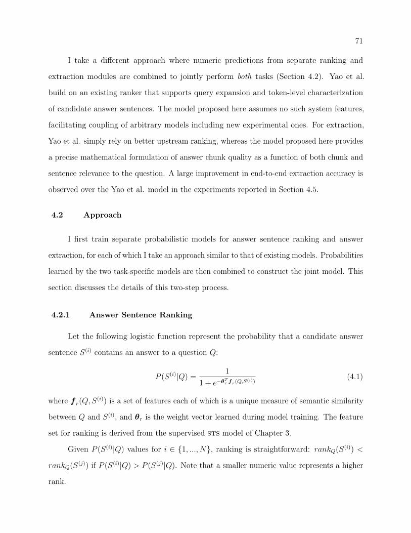
71

I take a different approach where numeric predictions from separate ranking and

extraction modules are combined to jointly perform both tasks (Section 4.2). Yao et al.

build on an existing ranker that supports query expansion and token-level characterization

of candidate answer sentences. The model proposed here assumes no such system features,

facilitating coupling of arbitrary models including new experimental ones. For extraction,

Yao et al. simply rely on better upstream ranking, whereas the model proposed here provides

a precise mathematical formulation of answer chunk quality as a function of both chunk and

sentence relevance to the question. A large improvement in end-to-end extraction accuracy is

observed over the Yao et al. model in the experiments reported in Section 4.5.

4.2 Approach

I first train separate probabilistic models for answer sentence ranking and answer

extraction, for each of which I take an approach similar to that of existing models. Probabilities

learned by the two task-specific models are then combined to construct the joint model. This

section discusses the details of this two-step process.

4.2.1 Answer Sentence Ranking

Let the following logistic function represent the probability that a candidate answer

sentence S(i) contains an answer to a question Q:

P (S(i)|Q) =1

1 + e−θTr fr(Q,S(i))

(4.1)

where f r(Q,S(i)) is a set of features each of which is a unique measure of semantic similarity

between Q and S(i), and θr is the weight vector learned during model training. The feature

set for ranking is derived from the supervised sts model of Chapter 3.

Given P (S(i)|Q) values for i ∈ {1, ..., N}, ranking is straightforward: rankQ(S(i)) <

rankQ(S(j)) if P (S(i)|Q) > P (S(j)|Q). Note that a smaller numeric value represents a higher

rank.

72

4.2.2 Answer Extraction

I follow the framework described in Algorithm 6 for answer extraction. Below is a

description of my implementation of the generic steps:

• Step 2: I adopt the strategy proposed by Severyn and Moschitti [81] of extracting

only the np chunks, for which I construct a base phrase chunker based on a small set

of regular expressions over pos tags.

• Step 4: The quality φ(c) of a candidate chunk c in S(i) is given by the following

logistic function:

φ(c) = P (c|Q,S(i)) =1

1 + e−θTe fe(Q,S(i),c)

(4.2)

where f e(Q,S(i), c) is the feature set for chunk c relative to Q, and θe is the weight

vector learned during model training. The feature set for extraction is described in

Section 4.4.

• Step 6: Given an existing set {G(1)C , ...,G

(M)C } of (possibly empty) chunk groups (i.e.

where each G(i)C is a multiset of semantically equivalent chunks), a new chunk c is

added to group G(i)C , if (1) all content words in c are in at least one member of G(i)

C ,

or (2) there exists a member of G(i)C all of whose content words are in c. If no such

group is found, a new group G(M+1)C is created with c as its only member.

• Step 10: The longest chunk in G(∗)C is extracted as the best answer C.

Additionally, I retain only the top t of all answer candidates extracted in step 5 to

prevent propagation of noisy chunks to later steps. The value of t is set using the Wang et al.

[104] dev set.

4.2.3 Joint Ranking and Extraction

The primary goal of the joint model is to facilitate the application of both chunk-level

and sentence-level features to ranking as well as extraction. To that end, it first computes the

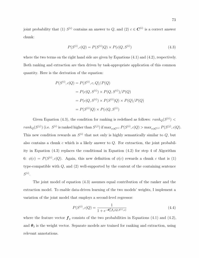
73

joint probability that (1) S(i) contains an answer to Q, and (2) c ∈ C(i) is a correct answer

chunk:

P (S(i), c|Q) = P (S(i)|Q)× P (c|Q,S(i)) (4.3)

where the two terms on the right hand side are given by Equations (4.1) and (4.2), respectively.

Both ranking and extraction are then driven by task-appropriate application of this common

quantity. Here is the derivation of the equation:

P (S(i), c|Q) = P (S(i), c, Q)/P (Q)

= P (c|Q,S(i))× P (Q,S(i))/P (Q)

= P (c|Q,S(i))× P (S(i)|Q)× P (Q)/P (Q)

= P (S(i)|Q)× P (c|Q,S(i))

Given Equation (4.3), the condition for ranking is redefined as follows: rankQ(S(i)) <

rankQ(S(j)) (i.e. S(i) is ranked higher than S(j)) if maxc∈C(i) P (S(i), c|Q)>maxc∈C(j) P (S(j), c|Q).

This new condition rewards an S(i) that not only is highly semantically similar to Q, but

also contains a chunk c which is a likely answer to Q. For extraction, the joint probabil-

ity in Equation (4.3) replaces the conditional in Equation (4.2) for step 4 of Algorithm

6: φ(c) = P (S(i), c|Q). Again, this new definition of φ(c) rewards a chunk c that is (1)

type-compatible with Q, and (2) well-supported by the content of the containing sentence

S(i).

The joint model of equation (4.3) assumes equal contribution of the ranker and the

extraction model. To enable data-driven learning of the two models’ weights, I implement a

variation of the joint model that employs a second-level regressor:

P (S(i), c|Q) =1

1 + e−θT2 f2(Q,S(i),c)

(4.4)

where the feature vector f 2 consists of the two probabilities in Equations (4.1) and (4.2),

and θ2 is the weight vector. Separate models are trained for ranking and extraction, using

relevant annotations.

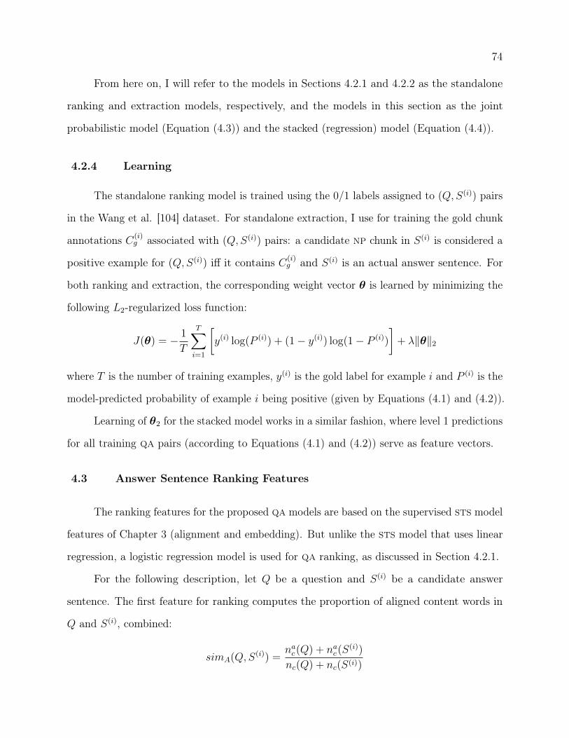
74

From here on, I will refer to the models in Sections 4.2.1 and 4.2.2 as the standalone

ranking and extraction models, respectively, and the models in this section as the joint

probabilistic model (Equation (4.3)) and the stacked (regression) model (Equation (4.4)).

4.2.4 Learning

The standalone ranking model is trained using the 0/1 labels assigned to (Q,S(i)) pairs

in the Wang et al. [104] dataset. For standalone extraction, I use for training the gold chunk

annotations C(i)g associated with (Q,S(i)) pairs: a candidate np chunk in S(i) is considered a

positive example for (Q,S(i)) iff it contains C(i)g and S(i) is an actual answer sentence. For

both ranking and extraction, the corresponding weight vector θ is learned by minimizing the

following L2-regularized loss function:

J(θ) = − 1

T

T∑i=1

[y(i) log(P (i)) + (1− y(i)) log(1− P (i))

]+ λ‖θ‖2

where T is the number of training examples, y(i) is the gold label for example i and P (i) is the

model-predicted probability of example i being positive (given by Equations (4.1) and (4.2)).

Learning of θ2 for the stacked model works in a similar fashion, where level 1 predictions

for all training qa pairs (according to Equations (4.1) and (4.2)) serve as feature vectors.

4.3 Answer Sentence Ranking Features

The ranking features for the proposed qa models are based on the supervised sts model

features of Chapter 3 (alignment and embedding). But unlike the sts model that uses linear

regression, a logistic regression model is used for qa ranking, as discussed in Section 4.2.1.

For the following description, let Q be a question and S(i) be a candidate answer

sentence. The first feature for ranking computes the proportion of aligned content words in

Q and S(i), combined:

simA(Q,S(i)) =nac(Q) + nac(S

(i))

nc(Q) + nc(S(i))

75

where nac(·) and nc(·) represent the number of aligned content words and the total number of

content words in a sentence, respectively.

S(i) can be arbitrarily long and still contain an answer to Q. In the above similarity

measure, longer answer sentences are penalized due to a larger number of unaligned words.

To counter this, a measure of coverage of Q by S(i) is employed as a second ranking feature:

covA(Q,S(i)) =nac(Q)

nc(Q)

The final ranking feature is the cosine similarity between the sentence embeddings of Q

and S(i):

simE(Q,S(i)) =EQ ·ES(i)

|EQ||ES(i)|

where EQ and ES(i) are simply sums of content lemma embeddings [10] in Q and S(i),

respectively.

The alignment module in the ranker has two small implementation differences with the

sts aligner. First, unlike the sts aligner—which allows a single neighbor word to be matched

to multiple words in the other sentence during computation of contextual similarity—the

ranker matches neighbors using max-weighted bipartite matching, where word similarities

serve as edge weights. Second, while the sts aligner adopts a greedy best-first strategy

for aligning word pairs based on their final weights (derived from lexical and contextual

similarity), the ranker uses these weights as edge weights in a max-weighted bipartite matching

of word pairs.

4.4 Answer Extraction Features

As mentioned in Section 4.2.2, only np chunks are considered as answer candidates for

extraction in this study. The chunk features used in the proposed extraction models can

be categorized into two broad groups, which I describe in this section. For the following

discussion, let (Q,S(i), c) be our question, answer sentence, answer chunk triple.

76

4.4.1 Question-Independent Features

These features represent properties of c independent of the nature of Q. For example,

the first two proposed features fire if all content words in c are present in Q or align to words

in Q. Such chunks rarely contain an answer, regardless of the type of Q.

Yao et al. [107] report an observation that answer chunks often appear near aligned

content words of specific types in S(i). To model this phenomenon, I adopt their features

specifying the distance of c from the nearest aligned content word wa in S(i) and the

pos/dep/ner tags of wa. In addition, to encode the total amount of local evidence present

for c, the proportions of aligned content words in its dependency (size = 2) and surface (size

= 3) contexts in S(i) are used as features.

4.4.2 Features Containing the Question Type

The type of a trec-style factoid question is simply the question word (e.g., who, where)

or phrase (e.g., how many). The features discussed in this section are of the form “question-

type|x”, where x can be an elementary (i.e. unit) or composite feature. The rationale is that

certain features are informative primarily in the context of certain question types (e.g., a

likely answer to a when question is a chunk containing the ner tag DATE).

Headword Features. The headword of c is extracted and its pos/dep/ner tags are

used as as features (appended to the question type). A headword in the subject position of

S(i) or with PERSON as its ner tag, for example, is a likely answer to a who question.

Question Focus. The question focus word represents the entity about which the

question is being asked. For example, in What is the largest country in the world?,

the focus word is country. For question types like what and which, properties of the question

focus largely determine the nature of the answer. In the above example, the focus word

indicates that GPE is a likely ner tag for the answer.

The question focus is extracted using a rule-based system originally designed for a

77

(question-type, question-focus-word, headword-pos-tag)(question-type, question-focus-word, headword-dep-tag)(question-type, question-focus-word, headword-ner-tag)

(question-type, question-focus-pos-tag, headword-pos-tag)(question-type, question-focus-pos-tag, headword-dep-tag)(question-type, question-focus-pos-tag, headword-ner-tag)(question-type, question-focus-ner-tag, headword-pos-tag)(question-type, question-focus-ner-tag, headword-dep-tag)(question-type, question-focus-ner-tag, headword-ner-tag)

Table 4.2: Answer extraction features derived from (1) the question type, (2) the questionfocus word and its pos/ner tags, and (3) the pos/dep/ner tags of the answer chunkheadword.

different application, under the assumption that a question could span multiple sentences.

The rule-based system is loosely inspired by the work of Lally et al. [54], from which it differs

radically because the questions in the Jeopardy! game are expressed as answers. The focus

extractor first determines the question word or words, which is then used in conjunction with

the parse tree to decide whether the question word itself or some other word in the sentence

is the actual focus.

I pair the headword’s pos/dep/ner tags with the focus word and its pos/ner tags,

and add each such pair (appended to the question type) to the feature set. There are nine

features here, as shown in Table 4.2.

The true/false labels of the following propositions are also included in the feature

set (in conjunction with the question type): (1) the question focus word is in c, (2) the

question focus pos tag is in the pos tags of c, and (3) the question focus ner tag is of

the form x or x_DESC, and x is in the ner tags of c, for some x (e.g., GPE). The answer to

the question Which university has won the most Nobel prizes?, for example, is likely

to contain the word University—the feature in (1) can thus be useful in answering such

questions. As another example, in the question In what country did the Khmer Rouge

movement take place?, the question focus word is country with an ner tag GPE_DESC; the

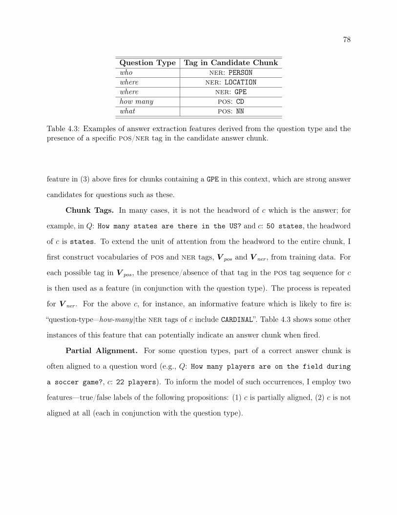
78

Question Type Tag in Candidate Chunkwho ner: PERSONwhere ner: LOCATIONwhere ner: GPEhow many pos: CDwhat pos: NN

Table 4.3: Examples of answer extraction features derived from the question type and thepresence of a specific pos/ner tag in the candidate answer chunk.

feature in (3) above fires for chunks containing a GPE in this context, which are strong answer

candidates for questions such as these.

Chunk Tags. In many cases, it is not the headword of c which is the answer; for

example, in Q: How many states are there in the US? and c: 50 states, the headword

of c is states. To extend the unit of attention from the headword to the entire chunk, I

first construct vocabularies of pos and ner tags, V pos and V ner, from training data. For

each possible tag in V pos, the presence/absence of that tag in the pos tag sequence for c

is then used as a feature (in conjunction with the question type). The process is repeated

for V ner. For the above c, for instance, an informative feature which is likely to fire is:

“question-type=how-many |the ner tags of c include CARDINAL”. Table 4.3 shows some other

instances of this feature that can potentially indicate an answer chunk when fired.

Partial Alignment. For some question types, part of a correct answer chunk is

often aligned to a question word (e.g., Q: How many players are on the field during

a soccer game?, c: 22 players). To inform the model of such occurrences, I employ two

features—true/false labels of the following propositions: (1) c is partially aligned, (2) c is not

aligned at all (each in conjunction with the question type).

79

Dataset # Questions # qa Pairs % Positivetrain-all 1,229 53,417 12.0

train 94 4,718 7.4dev 82 1,148 19.3test 100 1,517 18.7

Table 4.4: Summary of the Wang et al. [104] corpus.

4.5 Experiments

4.5.1 Data

The Wang et al. [104] corpus is created from Text REtrieval Conference (trec) 8–13

qa data. It consists of a set of factoid questions, and for each question, a set of candidate

answer sentences. Each answer candidate is automatically drawn from a larger document

based on two selection criteria: (1) a non-zero content word overlap with the question, or (2)

a match with the gold regexp answer pattern for the question (training only).

train pairs are drawn from trec 8–12; dev and test pairs are drawn from trec

13. Details of the train/dev/test split are given in Table 4.4. train-all is a large set

of automatically judged (thus noisy) qa pairs: a sentence is considered a positive example

if it matches the gold answer pattern for the corresponding question. train is a much

smaller subset of train-all, containing pairs that are manually corrected for errors. Manual

judgment is produced for all dev and test pairs, too.

For answer extraction, Yao et al. [107] add to each qa pair the correct answer chunk(s).

The gold trec patterns are used to first identify relevant chunks in each answer sentence.

train, dev and test are then manually corrected for errors.

The Wang et al. [104] dataset also comes with pos/dep/ner tags for each sentence.

They use the mxpost tagger [78] for pos tagging, the mstparser [63] to generate typed

dependency trees, and the bbn Identifinder [13] for ner tagging. Although more recent

80

parses and taggers are available that produce better output, this work aims to study the

effect of the proposed models and features on system performance, rather than on additional

variables; therefore, to support comparison with prior work, I use the tags provided with the

dataset for all experiments reported in this section.

4.5.2 Answer Sentence Ranking

The standard evaluation procedure and metrics for qa rankers reported in the literature

are adopted in the following experiments.

4.5.2.1 Evaluation Metrics

The metrics for ranking are Mean Average Precision (map) and Mean Reciprocal Rank

(mrr). Here I define both in terms of simpler metrics.

Precision at K. Given a question Q and a set of candidate answer sentences

{S(1), ..., S(N)}, let the output of a ranker be [R(1), ..., R(N)], so that each R(i) ∈ {S(1), ..., S(N)}

and the predicted rank of R(i) is higher than the predicted rank of R(j) whenever i < j. The

ranker’s precision at K for Q (PK(Q)) is then defined as the proportion of correct answer

sentences in the set {R(1), ..., R(K)}.

Average Precision. Let A be the set of correct answer sentences for Q in the

above scenario. Then the average precision (AP ) of the ranker for Q can be defined as:

AP (Q) = 1|A|∑

i:R(i)∈A Pi(Q).

Reciprocal Rank. In the above scenario, let j be the smallest index in {1, ..., N} such

that R(j) ∈ A. Then the reciprocal rank (RR) of the ranker for Q is: RR(Q) = Pj(Q) = 1/j.

map. The map of a ranker over a set of questions Q = {Q(1), ..., Q(M)} is defined as:

MAP (Q) = 1M

∑Mi=1AP (Q(i)).

mrr. The mrr of a ranker over a set of questions Q = {Q(1), ..., Q(M)} is defined as:

MRR(Q) = 1M

∑Mi=1RR(Q(i)).

81

Model map% mrr%trainShnarch [85] 68.60 75.40Yih et al. [111] 70.92 77.00Yu et al. [113] 70.58 78.00Severyn & Moschitti [82] 73.29 79.62

Proposed Standalone Model 76.05 83.99Proposed Joint Probabilistic Model 81.59 89.09Proposed Stacked Model 80.77 86.85train-allYu et al. [113] 71.13 78.46Severyn & Moschitti [82] 74.59 80.78

Proposed Standalone Model 75.68 83.09Proposed Joint Probabilistic Model 84.95 91.95Proposed Stacked Model 82.56 90.69

Table 4.5: Answer sentence ranking results.

4.5.2.2 Setup

For qa ranking, test questions that do not have both correct and incorrect candidate

answer sentences are irrelevant since any ranking is correct for such questions. Following past

qa rankers, I therefore remove such instances from dev and test. Of the original 1,517

test pairs, 1,442 (> 95%) are retained after this exclusion. I use the logistic regression

implementation of Scikit-learn [74] and use the Wang et al. [104] dev set to set C, the

regularization strength parameter. The standard trec_eval script is used to generate all

results.

4.5.2.3 Results

Table 4.5 shows performances of the proposed ranking models and recent baseline

systems on test. The proposed qa similarity features (i.e. the standalone ranker) based on

the supervised sts model features of Chapter 3 outperform all baselines with both train and

train-all, although the additional noisy examples in the latter are not found to improve

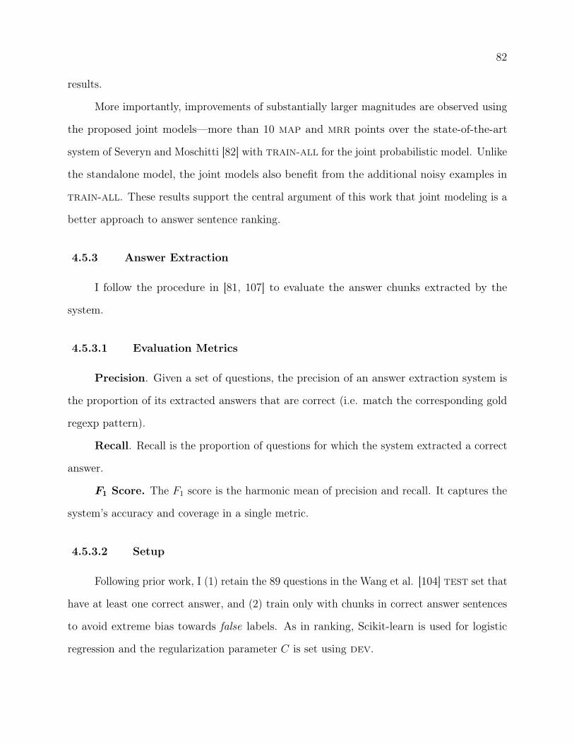
82

results.

More importantly, improvements of substantially larger magnitudes are observed using

the proposed joint models—more than 10 map and mrr points over the state-of-the-art

system of Severyn and Moschitti [82] with train-all for the joint probabilistic model. Unlike

the standalone model, the joint models also benefit from the additional noisy examples in

train-all. These results support the central argument of this work that joint modeling is a

better approach to answer sentence ranking.

4.5.3 Answer Extraction

I follow the procedure in [81, 107] to evaluate the answer chunks extracted by the

system.

4.5.3.1 Evaluation Metrics

Precision. Given a set of questions, the precision of an answer extraction system is

the proportion of its extracted answers that are correct (i.e. match the corresponding gold

regexp pattern).

Recall. Recall is the proportion of questions for which the system extracted a correct

answer.

F1 Score. The F1 score is the harmonic mean of precision and recall. It captures the

system’s accuracy and coverage in a single metric.

4.5.3.2 Setup

Following prior work, I (1) retain the 89 questions in the Wang et al. [104] test set that

have at least one correct answer, and (2) train only with chunks in correct answer sentences

to avoid extreme bias towards false labels. As in ranking, Scikit-learn is used for logistic

regression and the regularization parameter C is set using dev.

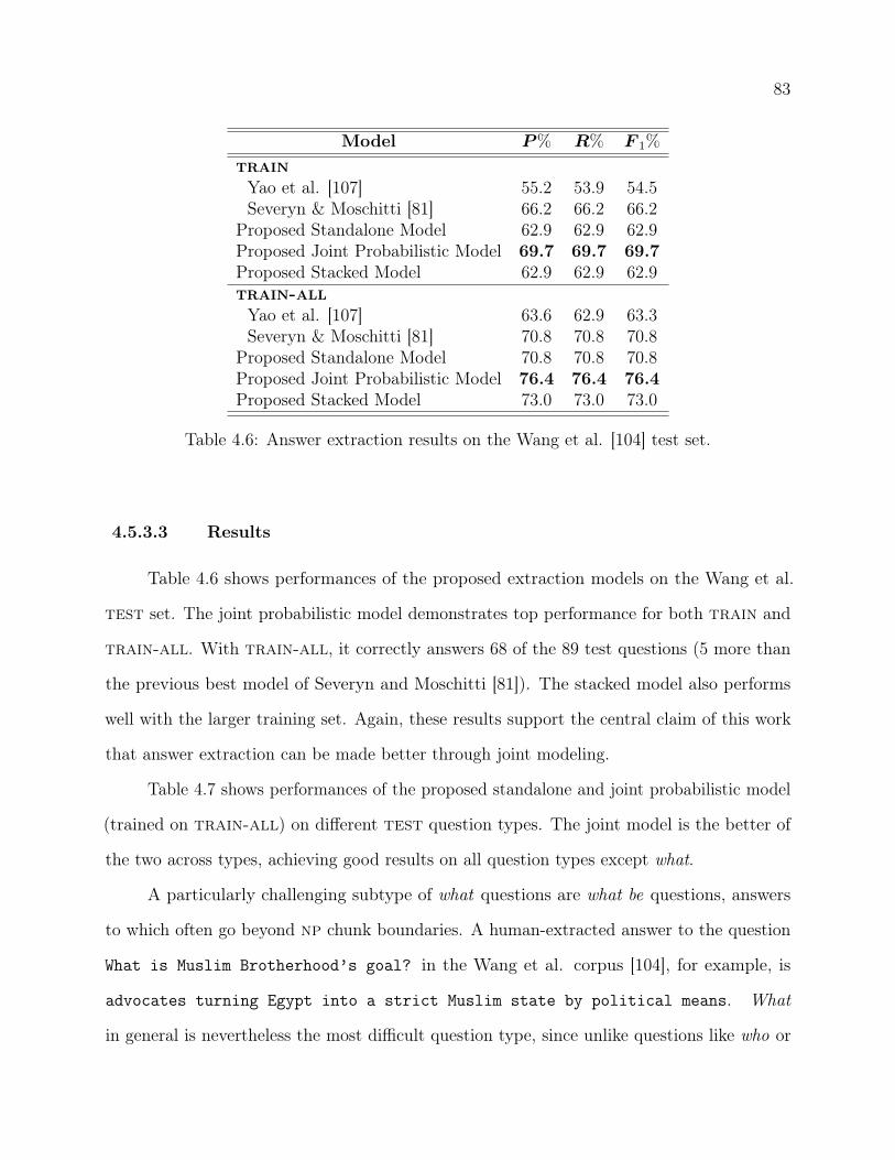
83

Model P% R% F 1%

trainYao et al. [107] 55.2 53.9 54.5Severyn & Moschitti [81] 66.2 66.2 66.2

Proposed Standalone Model 62.9 62.9 62.9Proposed Joint Probabilistic Model 69.7 69.7 69.7Proposed Stacked Model 62.9 62.9 62.9train-allYao et al. [107] 63.6 62.9 63.3Severyn & Moschitti [81] 70.8 70.8 70.8

Proposed Standalone Model 70.8 70.8 70.8Proposed Joint Probabilistic Model 76.4 76.4 76.4Proposed Stacked Model 73.0 73.0 73.0

Table 4.6: Answer extraction results on the Wang et al. [104] test set.

4.5.3.3 Results

Table 4.6 shows performances of the proposed extraction models on the Wang et al.

test set. The joint probabilistic model demonstrates top performance for both train and

train-all. With train-all, it correctly answers 68 of the 89 test questions (5 more than

the previous best model of Severyn and Moschitti [81]). The stacked model also performs

well with the larger training set. Again, these results support the central claim of this work

that answer extraction can be made better through joint modeling.

Table 4.7 shows performances of the proposed standalone and joint probabilistic model

(trained on train-all) on different test question types. The joint model is the better of

the two across types, achieving good results on all question types except what.

A particularly challenging subtype of what questions are what be questions, answers

to which often go beyond np chunk boundaries. A human-extracted answer to the question

What is Muslim Brotherhood’s goal? in the Wang et al. corpus [104], for example, is

advocates turning Egypt into a strict Muslim state by political means. What

in general is nevertheless the most difficult question type, since unlike questions like who or

84

Question Type Count ST JPwhat 37 51.4 56.8when 19 100.0 100.0where 11 100.0 90.9who/whom 10 60.0 70.0why 1 0.0 0.0how many 9 77.8 100.0how long 2 50.0 100.0

Table 4.7: F1% of the STandalone and the Joint Probabilistic extraction model across questiontypes.

when, answers do not have strict categories (e.g., a fixed set of ner tags).

4.5.3.4 Qualitative Analysis

I closely examine QA pairs for which the joint probabilistic model extracts a correct

answer chunk but the standalone model does not. Table 4.8 shows two such questions, with

two candidate answer sentences for each. Candidate answer chunks are boldfaced.

For the first question, only the sentence in row 1 contains an answer. The standalone

model assigns a higher score to the non-answer chunk in row 2, but the use of sentence-level

features enables the joint model to identify the more relevant chunk in row 1. Note that the

joint model score, being a product of two probabilities, is always lower than the standalone

model score. However, only the relative score matters here, as the chunk with the highest

overall score is eventually selected for extraction.

For the second question, both models compute a lower score for the non-answer chunk

Curt Newport than the answer chunk manned spacecraft. However, the incorrect chunk

appears in several candidate answer sentences (not shown here), resulting in a high overall

score for the standalone model (Algorithm 6: steps 7 and 8). The joint model assigns a much

lower score to each instance of this chunk due to weak sentence-level evidence, eventually

resulting in the extraction of the correct chunk.

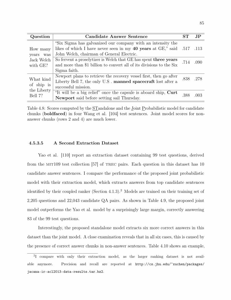
85

Question Candidate Answer Sentence ST JP

How manyyears wasJack Welchwith GE?

“Six Sigma has galvanized our company with an intensity thelikes of which I have never seen in my 40 years at GE,” saidJohn Welch, chairman of General Electric.

.517 .113

So fervent a proselytizer is Welch that GE has spent three yearsand more than $1 billion to convert all of its divisions to the SixSigma faith.

.714 .090

What kindof ship isthe LibertyBell 7?

Newport plans to retrieve the recovery vessel first, then go afterLiberty Bell 7, the only U.S . manned spacecraft lost after asuccessful mission.

.838 .278

“It will be a big relief” once the capsule is aboard ship, CurtNewport said before setting sail Thursday. .388 .003

Table 4.8: Scores computed by the STandalone and the Joint Probabilistic model for candidatechunks (boldfaced) in four Wang et al. [104] test sentences. Joint model scores for non-answer chunks (rows 2 and 4) are much lower.

4.5.3.5 A Second Extraction Dataset

Yao et al. [110] report an extraction dataset containing 99 test questions, derived

from the mit109 test collection [57] of trec pairs. Each question in this dataset has 10

candidate answer sentences. I compare the performance of the proposed joint probabilistic

model with their extraction model, which extracts answers from top candidate sentences

identified by their coupled ranker (Section 4.1.3).2 Models are trained on their training set of

2,205 questions and 22,043 candidate QA pairs. As shown in Table 4.9, the proposed joint

model outperforms the Yao et al. model by a surprisingly large margin, correctly answering

83 of the 99 test questions.

Interestingly, the proposed standalone model extracts six more correct answers in this

dataset than the joint model. A close examination reveals that in all six cases, this is caused by

the presence of correct answer chunks in non-answer sentences. Table 4.10 shows an example,

2I compare with only their extraction model, as the larger ranking dataset is not avail-

able anymore. Precision and recall are reported at http://cs.jhu.edu/~xuchen/packages/

jacana-ir-acl2013-data-results.tar.bz2.

86

Model P% R% F 1%

Yao et al. [110] 35.4 17.2 23.1Proposed Joint Probabilistic Model 83.8 83.8 83.8

Table 4.9: Performances of two joint extraction models on the Yao et al. [110] test set.

where the correct answer chunk Steve Sloan appears in all four candidate sentences, of

which only the first is actually relevant to the question. The standalone model assigns high

scores to all four instances and as a result observes a high overall score for the chunk. The

joint model, on the other hand, recognizes the false positives, and consequently observes a

smaller overall score for the chunk. However, this desired behavior eventually results in a

wrong extraction. These results have key implications for the evaluation of answer extraction

systems: metrics that assess performance on individual qa pairs can enable finer-grained

evaluation than that offered by end-to-end extraction metrics.

Candidate Answer Sentence ST JPAnother perk is getting to work with his son, Barry Van Dyke, who has aregular role as Detective Steve Sloan on “Diagnosis”. .861 .338

This is only the third time in school history the Raiders have begun a season6-0 and the first since 1976, when Steve Sloan, in his second season as coach,led them to an 8-0 start and 10-2 overall record.

.494 .010

He also represented several Alabama coaches, including Ray Perkins, BillCurry, Steve Sloan and Wimp Sanderson. .334 .007

Bart Starr, Joe Namath, Ken Stabler, Steve Sloan, Scott Hunter and WalterLewis are but a few of the legends on the wall of the Crimson Tide quarterbackscoach.

.334 .009

Table 4.10: Scores computed by the STandalone and the Joint Probabilistic model fornp chunks (boldfaced) in Yao et al. [110] test sentences for the question: Who is thedetective on “Diagnosis Murder”? The standalone model assigns high probabilities tonon-answer chunks in the last three sentences, subsequently corrected by the joint model.

87

4.6 Discussion

The proposed two-step approach to joint modeling, consisting of constructing separate

models for ranking and extraction first and then coupling their predictions, offers at least two

advantages. First, predictions from any given pair of ranking and extraction systems can be

combined, since such systems must compute a score for a qa pair or an answer chunk in order

to differentiate among candidates. Coupling of ranking and extraction systems in [81, 107],

for example, is straightforward within this framework. Second, this approach supports the

use of task-appropriate training data for ranking and extraction, which can provide a key

advantage. For example, while answer sentence ranking systems use both correct and incorrect

candidate answer sentences for model training, existing answer extraction systems discard

the latter in order to maintain a (relatively) balanced class distribution [81, 107]. Through

the separation of the ranking and extraction models during training, the proposed approach

naturally supports such task-specific sampling of training data.

A potentially limiting factor in the extraction model is the assumption that answers

are always expressed neatly in np chunks. While models that make no such assumption exist

(e.g., the crf model of Yao et al. [107]), extraction of long answers (such as the one discussed

in Section 4.5.3.3) is still difficult in practice due to their unconstrained nature.

4.7 Conclusions and Future Work

I present a joint model for the important qa tasks of answer sentence ranking and

answer extraction. By exploiting the interconnected nature of the two tasks, the model

demonstrates substantial performance improvements over previous best systems for both. The

sts features of Chapter 3 play a central role in the proposed ranking model and consequently

in the joint model.

An obvious direction for future work is the inclusion of new features for each task.

Answer sentence ranking, for example, can benefit from phrasal alignment and long-distance

88

context representation. Answer extraction for what questions can be made better using

a lexical answer type feature, or world knowledge (such as “blue is a color”) derived from

semantic networks like WordNet. The proposed joint model also facilitates straightforward

integration of features/predictions from other existing systems for both tasks, for example,

the convolutional neural sentence model in [82] for ranking. Finally, more sophisticated

techniques are required for extraction of the final answer chunk based on individual chunk

scores across QA pairs.

Chapter 5

Short Answer Grading using Text Similarity

Short-answer questions provide a useful means for eliciting student understanding of

specific concepts in a subject domain. Given a question and its correct answer, key measures

of the correctness of a student response can be derived from its semantic similarity with

the correct answer. Text similarity measures have been used in numerous short answer

grading systems [44, 68, 77]. From an application perspective, however, these systems vary

considerably along a set of key dimensions: amount of human effort involved, accuracy, speed,

and ease of implementation. Here I explore a design using the proposed sts features in

Chapter 3 that seeks to optimize performance along all these dimensions.

Textual similarity alone is inadequate as a measure of answer correctness. For example,

while the proposed sts system in Chapter 3 makes the general assumption that all content

words contribute equally to the meaning of a sentence, domain keywords (e.g., “mutation”

for biological evolution) are clearly more significant than arbitrary content words (e.g.,

“consideration”) for academic text. As another example, question demoting [68] proposes

to discard words that are present in the question text as a preprocessing step for grading.

Generic text similarity features are augmented with such grading-specific measures in the

proposed system.

I train a supervised model with the final feature set, which is evaluated on two different

grading tasks. The proposed model improves over the state of the art in each task. In

summary, the primary contribution of this study is a fast and accurate grading system

90

Question: What is the role of a prototype program in problem solving?Reference Answer: To simulate the behavior of portions of the desired software product.

Student Answers GradesA prototype program is used in problem solving to collect data for the problem. 1, 2It simulates the behavior of portions of the desired software product. 5, 5To find problem and errors in a program before it is finalized. 2, 2

Question: What are the main advantages associated with object-oriented programming?Reference Answer: Abstraction and reusability.

Student Answers GradesThey make it easier to reuse and adapt previously written code and they separate 5, 4complex programs into smaller, easier to understand classes.Object oriented programming allows programmers to use an object with classes that 1, 1can be changed and manipulated while not affecting the entire object at once.Reusable components, Extensibility, Maintainability, it reduces large problems into 4, 4smaller more manageable problems.

Table 5.1: Examples of short answer grades taken from [68].

requiring minimal human intervention that can be easily deployed and used as a base model

for further extension.

In the context of this dissertation, this chapter explores RQ4 of Section 1.3: How can

sts help in automatically grading short answers in academic tests?

5.1 sts and Short Answer Grading

When grading short-answer questions, human graders usually look for a very specific

set of concepts mentioned and/or described in a student response. One or more reference

answers provided by a domain expert in a natural language can describe such concepts. An

automated grader can then grade student responses based on their semantic similarity with

such reference answers. In this section, I use a set of examples to show this connection

between sts and short answer grading.

Table 5.1 shows two undergraduate Data Structures questions, their correct answers

and three different student answers to each. Each answer is graded by two human graders

91

on a scale of 0 to 5. These examples are taken from exams that were administered at the

University of North Texas [68]. For the first question, the student answer that receives a 5 out

of 5 from both graders is semantically almost identical to the reference answer, whereas the

other two answers are very dissimilar. The two high-scoring answers for question 2 specifically

mention reusability—one of the two key concepts in the reference answer, while providing a

description of the other concept—abstraction. The low-scoring answer, on the other hand,

neither mentions nor describes these two concepts. These examples show that given an sts

algorithm, simply by providing one or more reference answers, a lot of human effort could in

theory be saved that would otherwise be required to grade each individual student response.

In this chapter, I discuss the actual application of an sts model—the supervised model of

Chapter 3—to short answer grading.

5.2 Related Work

A comprehensive review of automatic short answer grading can be found in [18]. Here I

briefly discuss closely related work. Early work relied on patterns (e.g., regular expressions)

manually extracted from expert-provided reference answers [67, 71, 87]. Such patterns encode

key concepts representative of good answers. Use of manually designed patterns continues

to this day, such as [97], the winning system at the asap answer scoring contest.1 This is a

step requiring human intervention that natural language processing can help to eliminate.

Ramachandran et al. [77] propose a mechanism to automate the extraction of patterns from

the reference answer as well as high-scoring student answers. I adopt the simpler notion of

semantic alignment to avoid explicitly generating complicated patterns altogether.

Direct semantic matching (as opposed to pattern generation) has been explored in early

work like [55]. With advances in nlp techniques, this approach has gained popularity over

time [44, 51, 68, 69]. Such systems typically use a large set of similarity measures as features

for a supervised learning model. Features range from string similarity measures like word

1https://www.kaggle.com/c/asap-sas/

92

and character n-gram overlap to deeper semantic similarity measures based on resources

like WordNet and distributional methods like latent semantic analysis (lsa). However, a

large feature set contributes to higher system runtime and implementation difficulty. While

following this generic framework, I seek to improve on these criteria by adopting a minimal

set of core similarity features from the supervised sts model of Chapter 3. These features

also yield higher accuracy by utilizing more recent measures of lexical similarity [10, 37],

shown to outperform traditional resources and methods like WordNet, lsa, and disco [53].

As mentioned before, short-text semantic similarity has seen major progress in recent

times, due largely to the SemEval Semantic Textual Similarity task [1, 2, 3, 4]. The large

volume of systems evaluated at SemEval can serve as a source of important new features and

design elements for automatic short answer graders [8, 42, 43, 59].

Surprisingly, few existing grading systems utilize simple and computationally inexpensive

grading-specific techniques like question demoting [68] and term weighting. The proposed

model augments the similarity features with these techniques.

5.3 Method

Following feature extraction, the proposed system trains a supervised model for grading.

As discussed in Section 5.4, this can be a regressor or a classifier depending on the task. This

section describes the features. Specifics of the models are given in Section 5.4.

5.3.1 Features

5.3.1.1 Text Similarity

Let R be the reference answer and S be the student answer.

Alignment. The first feature is taken directly from the supervised sts system of

Chapter 3: the proportion of content words in R and S that are aligned by the unsupervised

aligner of Chapter 2. To avoid penalizing long student responses that still contain the correct

93

answer, I also employ a second version of this feature: the proportion of aligned content

words only in R. From here on, I refer to this feature as coverage of the reference answer’s

content by the student response.

Semantic Vector Similarity. This feature is also taken directly from the supervised

sts model: cosine similarity between the R and S vectors, derived from word embeddings of

Baroni et al. [10].

5.3.1.2 Question Demoting

Each of the above similarity features is recomputed after removing from both the

reference answer and the student response words that appear in the question text. The

objective is to avoid rewarding a student response for repeating question words.

5.3.1.3 Term Weighting

To distinguish between domain keywords and arbitrary content words, in the next set

of features, a weight is assigned to every content word in the input sentences based on a

variant of tf-idf. While general short-text similarity models typically use only idf (inverse

document frequency) to penalize general words, the domain-specific nature of answer grading

also enables the application of a tf (term frequency) measure.

To fully automate the process for a question and reference answer pair, all content

words in the pair are identified. The top ten Wikipedia pages related to these words are

retrieved using the Google api. Each page is read along with all linked pages crawled using

Scrapy [70]. The in-domain term frequency (tf d) of a word in the answer is then computed

by extracting its raw count in this collection of pages. The same set of tools are used to

automatically extract Wikipedia pages in 25 different domains such as Art, Mathematics,

Religion, and Sport. A total of 14,125 pages are retrieved, occurrences in which are used to

compute the idf of each word.

I augment the alignment features—both original and question-demoted—with term

94

weights to generate new features. Each word is assigned a weight equal to its tf d×idf score.

The sum of weights is computed for (1) aligned, and (2) all content words in the reference

answer (after question demoting, if applicable). The ratio of these two numbers is then used

as a feature. I compute only coverage features (Section 5.3.1.1) to avoid computing term

weights for each student response. Thus the process of crawling and reading the documents

is performed once per question; all student responses can subsequently be graded quickly.

5.3.1.4 Length Ratio

The ratio of the number of words in the student response to that in the reference answer

is used as the final feature. The aim is to roughly capture whether or not the student response

contains enough detail.

5.4 Experiments

I evaluate the above features on two grading tasks. The first task, proposed by Mohler

et al. [68], asks one to compute a real-valued score for a student response on a scale of 0 to

5. The second task, proposed at SemEval-2013 [31], asks one to assign a label (e.g., correct

or irrelevant) to a student response that shows how appropriate it is as an answer to the

question. Thus from a machine learning perspective, the first is a regression task and the

second is a classification task. Results are discussed below.

5.4.1 The Mohler et al. [68] Task

The dataset for this task consists of 80 undergraduate Data Structures questions and

2,273 student responses graded by two human judges. These questions are spread across ten

different assignments and two tests, each on a related set of topics (e.g., programming basics,

sorting algorithms, etc.). A reference answer is provided for each question. Inter-annotator

agreement was 58.6% (Pearson’s ρ) and .659 (root-mean-square error (rmse) on a 5-point

95

System Pearson’s r rmsetf-idf .327 1.022Lesk .450 1.050Mohler et al. [68] .518 .978Our Model .592 .887

Table 5.2: Performance on the Mohler et al. [68] dataset with out-of-domain training.Performances of simpler bag-of-words models are reported by those authors.

scale). Average of the two human scores is used as the final gold score for each student

answer.

I train a ridge regression model (Scikit-learn [74]) for each assignment and test using

annotations from the rest as training examples. A dev assignment or test is randomly

held out for model selection. Out-of-range output scores, if any, are rounded to the nearest

in-range integer. Following Mohler et al. [68], I compute a single Pearson correlation and

rmse score over all student responses from all datasets. Average results across 1,000 runs

of the system are shown in Table 5.2. The proposed model shows a large and significant

performance improvement over the state-of-the-art model of Mohler et al. (two-tailed t-test,

p <.001). Their system employs a support vector machine that predicts scores using a set

of dependency graph alignment and lexical similarity measures. The proposed features are

similar in intent, but are based on latest advances in lexical similarity and monolingual

alignment.

Ramachandran et al. [77] adopt a different setup to evaluate their model on the same

dataset. For each assignment/test, they use 80% of the data for training and the rest as test.

This setup thus enables in-domain model training. Their system automatically generates

regexp patterns intended to capture semantic variations and syntactic structures of good

answers. Features derived from matches with such patterns (e.g., content word similarity and

word order match) as well as term frequencies in the student response are used to train a set

96

System r rmseRamachandran et al. [77] .61 .86Our Model .63 .85

Table 5.3: Performance on the Mohler et al. [68] dataset with in-domain training.

of random forest regressors, whose predictions are then combined to output a single score.

Results in this setup are shown in Table 5.3. Again, averaged over 1,000 runs, the proposed

model performs better on both evaluation metrics. The differences are smaller than before

but still statistically significant (two-tailed t-test, p <.001).

5.4.2 The SemEval-2013 Task

Instead of a real-valued score, this task asks one to assign one of five labels to a student

response: correct, partially correct/incomplete, contradictory, irrelevant, and non-domain (an

answer that contains no domain content). I use the SciEntsBank corpus, containing 9,804

answers to 197 questions in 15 science domains. Of these, 3,969 are used for model training

and the remaining 5,835 for test. A reference answer is provided for each question.

The test set is divided into three subsets with varying degrees of similarity with the

training examples. The Unseen Answers (ua) dataset consists of responses to questions that

are present in the training set. Unseen Questions (uq) contains responses to in-domain but

previously unseen questions. Three of the fifteen domains were held out for a final Unseen

Domains (ud) test set, containing completely out-of-domain question-response pairs. For

this task, I train a random forest classifier with 500 trees in Scikit-learn using the proposed

feature set.

Table 5.4 shows the performance of the proposed model (averaged over 100 runs) along

with that of top systems2 at SemEval-2013 (and of simpler baselines). ets [44] employs a

2Systems with best overall performance on SciEntsBank.

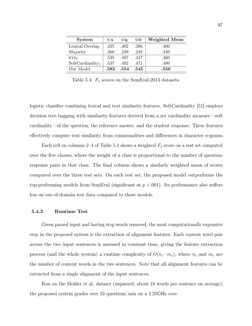
97

System ua uq ud Weighted MeanLexical Overlap .435 .402 .396 .400Majority .260 .239 .249 .249ets1 .535 .487 .447 .460SoftCardinality1 .537 .492 .471 .480Our Model .582 .554 .545 .550

Table 5.4: F1 scores on the SemEval-2013 datasets.

logistic classifier combining lexical and text similarity features. SoftCardinality [51] employs

decision tree bagging with similarity features derived from a set cardinality measure—soft

cardinality—of the question, the reference answer, and the student response. These features

effectively compute text similarity from commonalities and differences in character n-grams.

Each cell on columns 2–4 of Table 5.4 shows a weighted F1-score on a test set computed

over the five classes, where the weight of a class is proportional to the number of question-

response pairs in that class. The final column shows a similarly weighted mean of scores

computed over the three test sets. On each test set, the proposed model outperforms the

top-performing models from SemEval (significant at p <.001). Its performance also suffers

less on out-of-domain test data compared to those models.

5.4.3 Runtime Test

Given parsed input and having stop words removed, the most computationally expensive

step in the proposed system is the extraction of alignment features. Each content word pair

across the two input sentences is assessed in constant time, giving the feature extraction

process (and the whole system) a runtime complexity of O(nc ·mc), where nc and mc are

the number of content words in the two sentences. Note that all alignment features can be

extracted from a single alignment of the input sentences.

Run on the Mohler et al. dataset (unparsed; about 18 words per sentence on average),

the proposed system grades over 33 questions/min on a 2.25GHz core.

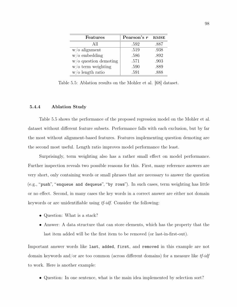
98

Features Pearson’s r rmseAll .592 .887

w/o alignment .519 .938w/o embedding .586 .892w/o question demoting .571 .903w/o term weighting .590 .889w/o length ratio .591 .888

Table 5.5: Ablation results on the Mohler et al. [68] dataset.

5.4.4 Ablation Study

Table 5.5 shows the performance of the proposed regression model on the Mohler et al.

dataset without different feature subsets. Performance falls with each exclusion, but by far

the most without alignment-based features. Features implementing question demoting are

the second most useful. Length ratio improves model performance the least.

Surprisingly, term weighting also has a rather small effect on model performance.

Further inspection reveals two possible reasons for this. First, many reference answers are

very short, only containing words or small phrases that are necessary to answer the question

(e.g., “push”, “enqueue and dequeue”, “by rows”). In such cases, term weighting has little

or no effect. Second, in many cases the key words in a correct answer are either not domain

keywords or are unidentifiable using tf-idf. Consider the following:

• Question: What is a stack?

• Answer: A data structure that can store elements, which has the property that the

last item added will be the first item to be removed (or last-in-first-out).

Important answer words like last, added, first, and removed in this example are not

domain keywords and/or are too common (across different domains) for a measure like tf-idf

to work. Here is another example:

• Question: In one sentence, what is the main idea implemented by selection sort?

99

• Answer: Taking one array element at a time, from left to right, it identifies the

minimum from the remaining elements and swaps it with the current element.

Again, while the important answer word swap perhaps qualifies as a domain keyword, other

important words like left, right, minimum, and current do not.

5.5 Conclusions

This chapter presents a fast, easily replicable and high-performance short answer grading

system based on the sts features proposed in Chapter 3. Augmented with grading-specific

measures, the system demonstrates top results on multiple benchmarks. There is, however,

immense scope for improvement. Subtle factors like differences in modality or polarity might

go undetected with coarse text similarity measures. Inclusion of text-level paraphrase and

entailment features can help in such cases. Additional term weighting mechanisms are needed

to identify important answer words in many cases. The proposed system provides a simple

base model that can be easily extended with new features for more accurate answer grading.

The grader is available at https://github.com/ma-sultan/short-answer-grader.

Chapter 6

Domain Adaptation for Short Text Similarity

sts has applications in numerous downstream tasks (Chapter 1), with input text from

disparate sources such as news headlines, academic text, and tweets. When building a

supervised sts model for a new domain (a previously unseen source of text, for example),

training on data from other domains may or may not be useful. For instance, the supervised

sts model of Chapter 3 performs much better on the SemEval-2012 msrpar-test dataset

when trained on in-domain annotations than on out-of-domain ones (Table 3.7). On the other

hand, large amounts of out-of-domain training data can be useful when in-domain examples

are scarce. The goal of this chapter is to explore supervised domain adaptation (da) for

sts: a technique that utilizes all available training examples from all domains for model

training, but distinguishes between in-domain and out-of-domain data.

While the term “domain” can take a range of meanings, I consider adaptation to different

(1) sources of text (e.g., news headlines, forum qa), and (2) applications of sts (qa and

answer grading). The goal is to improve performance in a target domain with few in-domain

annotations by using many out-of-domain ones. Following the machine learning literature, I

will also use the term multitask learning (mtl) for adaptation to different applications

from here on.

I explore a Bayesian approach that expands a base linear sts model—the supervised

model presented in Chapter 3—for da and mtl. Given training examples from different

domains, it learns a single global instance of the base model’s parameter vector (i.e. the

101

weights of the alignment and the embedding features), as well as domain-specific instances—

one for each domain. The generative model posits that (1) each domain-specific instance

directly generates the observations in the corresponding domain, and (2) all domain-specific

instances share the global instance as a common Gaussian prior. This shared prior enables

information transfer across domains. Importantly, this idea can be extended with little effort

to a nested domain hierarchy (domains within domains), which enables the construction of

a single, unified sts model that generalizes across domains as well as tasks, capturing the

nuances that an sts system must have for tasks such as short answer scoring or question

answering.

I compare the proposed da and mtl methods against two baselines: (1) a domain-

agnostic model that uses all training data and does not distinguish between in-domain and

out-of-domain examples, and (2) a model that learns only from in-domain examples. Across

ten different sts domains, the adaptive model consistently outperforms the first baseline

while performing at least as well as the second across training datasets of different sizes. The

mtl model also yields better overall results over the same baselines across three related tasks:

(1) sts, (2) short answer scoring (sas), and (3) answer sentence ranking (asr) for question

answering.

Studies reported in this chapter are designed to answer research question 5 of Section 1.3:

How can sts algorithms adapt to requirements of different target domains and

applications?

6.1 Tasks and Datasets

The three tasks in focus (sts, sas, and asr) have been discussed in detail in Chapters

3 through 5. Here I provide a quick recap, and discuss the specific selection of data for the

experiments reported in this chapter.

Short Text Similarity (sts) Given two short pieces of text, the goal of sts is to

provide a real-valued score that represents their degree of semantic similarity. As in Chapter 3,

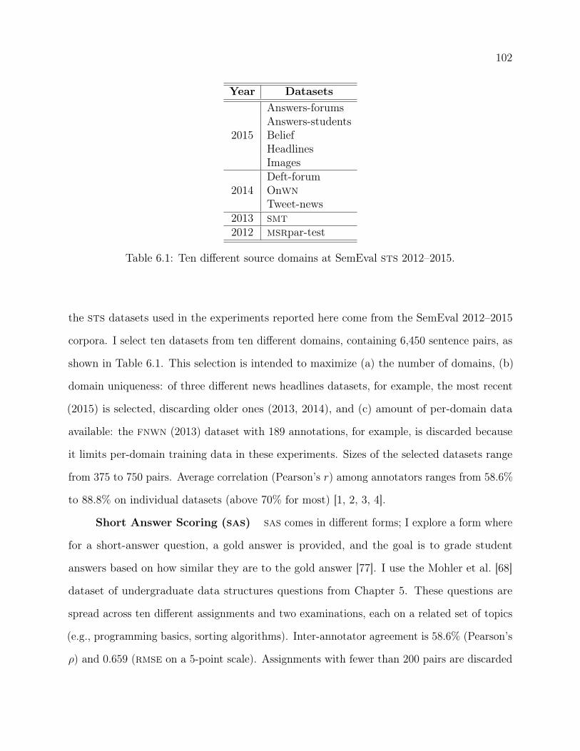
102

Year Datasets

2015

Answers-forumsAnswers-studentsBeliefHeadlinesImages

2014Deft-forumOnwnTweet-news

2013 smt2012 msrpar-test

Table 6.1: Ten different source domains at SemEval sts 2012–2015.

the sts datasets used in the experiments reported here come from the SemEval 2012–2015

corpora. I select ten datasets from ten different domains, containing 6,450 sentence pairs, as

shown in Table 6.1. This selection is intended to maximize (a) the number of domains, (b)

domain uniqueness: of three different news headlines datasets, for example, the most recent

(2015) is selected, discarding older ones (2013, 2014), and (c) amount of per-domain data

available: the fnwn (2013) dataset with 189 annotations, for example, is discarded because

it limits per-domain training data in these experiments. Sizes of the selected datasets range

from 375 to 750 pairs. Average correlation (Pearson’s r) among annotators ranges from 58.6%

to 88.8% on individual datasets (above 70% for most) [1, 2, 3, 4].

Short Answer Scoring (sas) sas comes in different forms; I explore a form where

for a short-answer question, a gold answer is provided, and the goal is to grade student

answers based on how similar they are to the gold answer [77]. I use the Mohler et al. [68]

dataset of undergraduate data structures questions from Chapter 5. These questions are

spread across ten different assignments and two examinations, each on a related set of topics

(e.g., programming basics, sorting algorithms). Inter-annotator agreement is 58.6% (Pearson’s

ρ) and 0.659 (rmse on a 5-point scale). Assignments with fewer than 200 pairs are discarded

103

in the sas experiments reported in this chapter, retaining 1,182 student responses to 40

questions spread across five assignments and tests: Assignments #1, #2, and #3, and Exams

#11 and #12.

Answer Sentence Ranking (asr) Given a factoid question and a set of candidate

answer sentences, asr orders candidates so that sentences containing the answer are ranked

higher. Text similarity is the foundation of most prior work: a candidate sentence’s relevance

is based on its similarity with the question [82, 104, 107]. For experiments, I again use the

factoid questions developed by Wang et al. [104] from Text REtrieval Conferences (trec)

8–13. Candidate qa pairs of a question and a candidate were labeled with whether the

candidate answers the question. The questions are of different types (e.g., what, where); I

retain 2,247 qa pairs under four question types (what, when, who and how many), each with

at least 200 answer candidates in the combined development and test sets. Each question

type represents a unique topical domain—who questions are about persons and how many

questions are about quantities.

6.2 Bayesian Domain Adaptation for sts

I first discuss the base linear models for the three tasks: Bayesian L2-regularized linear

(for sts and sas) and logistic (for asr) regression. These models are then extended for (1)

adaptation across different short text similarity domains, and (2) multitask learning of short

text similarity (sts), short answer scoring (sas), and answer sentence ranking (asr).

6.2.1 Base Models

In the base models (Figure 6.1), the feature vector f combines with the feature weight

vector w (including a bias term w0) to form predictions. Each parameter wi ∈ w has its own

zero-mean Gaussian prior with its standard deviation σwidistributed uniformly in [0,mσw ],

the covariance matrix Σw is diagonal, and the zero-mean prior L2 regularizes the model.

In the linear model (Figure 6.1a), S is the output (similarity score for sts; answer

104

𝑚𝜎w 𝝈w

Σw

wS𝜎𝑆

𝑚𝜎𝑆 f

𝜎𝑆 ~ 𝑈 0,𝑚𝜎𝑆

𝝈w ~ 𝑈 𝟎,𝑚𝜎w

Σw = 𝑑𝑖𝑎𝑔 𝝈w

w ~ 𝑁 𝟎, Σw

S ~ 𝑁 w𝑇f, 𝜎𝑆2

(a) Bayesian ridge regression for sts and sas.

𝑚𝜎w 𝝈w𝝈w ~ 𝑈 𝟎,𝑚𝜎w

Σw = 𝑑𝑖𝑎𝑔 𝝈w

w ~ 𝑁 𝟎, Σwp = 𝑆𝑖𝑔𝑚𝑜𝑖𝑑 w𝑇f

A ~ 𝐵𝑒𝑟𝑛𝑜𝑢𝑙𝑙𝑖 𝑝

p

A

f Σw

w

(b) Bayesian logistic regression for asr.

Figure 6.1: Base models for sts, sas and asr. Plates represent replication across sentencepairs.

score for sas), and is normally distributed around the weighted sum of features wTf . The

model error σS has a uniform prior over a prespecified range [0,mσS ]. In the logistic model

(Figure 6.1b) for asr, the probability p that the candidate sentence answers the question,

is (1) the sigmoid of wTf , and (2) the Bernoulli prior of A, whether or not the candidate

answers the question.

The common vectors w and f in these models enable joint parameter learning and

105

𝝈w∗~ 𝑈 𝟎,𝑚𝜎w∗

Σw∗= 𝑑𝑖𝑎𝑔 𝝈w∗

w∗ ~ 𝑁 𝟎, Σw∗

𝑚𝜎w∗

Σw∗

𝑚𝜎w

𝝈w𝝈w ~ 𝑈 𝟎,𝑚𝜎w

Σw Σw = 𝑑𝑖𝑎𝑔 𝝈w

w∗ w𝑑

w𝑑 ~ 𝑁 w∗, Σw

𝝈w∗

f

S𝑚𝜎𝑆 𝜎𝑆

𝜎𝑆 ~ 𝑈 0,𝑚𝜎𝑆 S ~ 𝑁 w𝑑𝑇f, 𝜎𝑆

2

Figure 6.2: Adaptation to different sts domains. The outer plate represents replication acrossdomains. Joint learning of a global weight vector w∗ along with individual domain-specificvectors wd enables inductive transfer among domains.

consequently multitask learning (Section 6.2.3).

6.2.2 Adaptation to sts Domains

Domain adaptation for the linear model (Figure 6.1a) learns a separate weight vector

wd for each domain d (i.e., applied to similarity computations for test pairs in domain

d) alongside a common, global domain-agnostic weight vector w∗, which has a zero-mean

Gaussian prior and serves as the Gaussian prior mean for each wd. Figure 6.2 shows the

model. Both w∗ and wd have hyperpriors identical to w in Figure 6.1a.1

Each wd depends not just on its domain-specific observations but also on information

derived from the global, shared parameter w∗. The balance between capturing in-domain

1Results do not improve with individual domain-specific instances of σS and σw, consistent with [35] for

dependency parsing and named entity recognition.

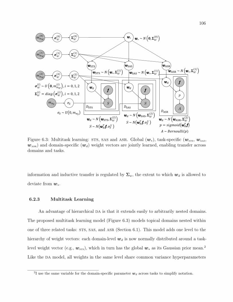
106

𝐷ASR

𝐷SAS𝐷STS

𝑚𝜎w(0)

𝑚𝜎w(1)

𝑚𝜎w(2)

𝝈w(𝑖)

~ 𝑈 𝟎,𝑚𝜎w(𝑖)

, 𝑖 = 0, 1, 2

𝚺w(𝑖)

= 𝑑𝑖𝑎𝑔 𝝈w𝑖

, 𝑖 = 0, 1, 2

𝝈w(0)

𝝈w(1)

𝝈w(2)

𝚺w(0)

𝚺w(1)

𝚺w(2)

𝑚𝜎𝑆 𝜎𝑆

𝜎𝑆 ~ 𝑈 0,𝑚𝜎𝑆

w∗ ~ 𝑁 𝟎, 𝚺w(0)

wSTS ~ 𝑁 w∗, 𝚺w(1)

wSAS ~ 𝑁 w∗, 𝚺w(1) wASR ~ 𝑁 w∗, 𝚺w

(1)

w∗

wSTS wSAS wASR

w𝑑f

S

f

S

w𝑑 ~ 𝑁 wSTS, 𝚺w(2)

S ~ 𝑁 w𝑑𝑇f, 𝜎𝑆

2

w𝑑 ~ 𝑁 wSAS, 𝚺w(2)

S ~ 𝑁 w𝑑𝑇f, 𝜎𝑆

2w𝑑 ~ 𝑁 wASR, 𝚺w

(2)

𝑝 = 𝑠𝑖𝑔𝑚𝑜𝑖𝑑 w𝑑𝑇f

𝐴 ~ 𝐵𝑒𝑟𝑛𝑜𝑢𝑙𝑙𝑖(𝑝)

w𝑑

w𝑑 f

p

A

Figure 6.3: Multitask learning: sts, sas and asr. Global (w∗), task-specific (wsts, wsas,wasr) and domain-specific (wd) weight vectors are jointly learned, enabling transfer acrossdomains and tasks.

information and inductive transfer is regulated by Σw, the extent to which wd is allowed to

deviate from w∗.

6.2.3 Multitask Learning

An advantage of hierarchical da is that it extends easily to arbitrarily nested domains.

The proposed multitask learning model (Figure 6.3) models topical domains nested within

one of three related tasks: sts, sas, and asr (Section 6.1). This model adds one level to the

hierarchy of weight vectors: each domain-level wd is now normally distributed around a task-

level weight vector (e.g., wsts), which in turn has the global w∗ as its Gaussian prior mean.2

Like the da model, all weights in the same level share common variance hyperparameters

2I use the same variable for the domain-specific parameter wd across tasks to simplify notation.

107

𝐷ASR𝐷STS ∪ 𝐷SAS𝜎𝑆 ~ 𝑈 0,𝑚𝜎𝑆

S ~ 𝑁 w𝑇f, 𝜎𝑆2

𝑚𝜎w

𝝈w Σw w

w ~ 𝑁 𝟎, Σw

𝝈w ~ 𝑈 𝟎,𝑚𝜎wΣw = 𝑑𝑖𝑎𝑔 𝝈w

𝑚𝜎𝑆

𝜎𝑆

f

S

f

p

A

p = 𝑆𝑖𝑔𝑚𝑜𝑖𝑑 w𝑇f

A ~ 𝐵𝑒𝑟𝑛𝑜𝑢𝑙𝑙𝑖 𝑝

Figure 6.4: A non-hierarchical joint model for sts, sas and asr. A common weight vectorw is learned for all tasks and domains.

while those across different levels are separate.

Again, this hierarchical structure (1) jointly learns global, task-level and domain-level

feature weights enabling inductive transfer among tasks and domains while (2) retaining

the distinction between in-domain and out-of-domain annotations. A task-specific model

(Figure 6.1) that only learns from in-domain annotations supports only (2). On the other

hand, a non-hierarchical joint model (Figure 6.4) supports only (1): it learns a single shared

w applied to any test pair regardless of task or domain. These models are compared in

Section 6.4.

6.3 Features

The feature set of the supervised sts model of Chapter 3 is used in the experiments

reported below. Given input sentences S(1) = (w(1)1 , ..., w

(1)n ) and S(2) = (w

(2)1 , ..., w

(2)m ) (where

each w is a token), the first feature is the proportion of content words in S(1) and S(2) that are

aligned by the unsupervised aligner of Chapter 2. To avoid penalizing long answer snippets

108

Task Current soa Proposed Bayesian Modelsts Pearson’s r = 73.6% Pearson’s r = 73.7%

sasPearson’s r = 51.8% Pearson’s r = 56.4%

rmse = 19.6% rmse = 18.1%

asrmap = 74.6% map = 76.0%mrr = 80.8% mrr = 82.8%

Table 6.2: The proposed Bayesian base models outperform the state of the art in sts, sasand asr.

(that still have the desired semantic content) in sas and asr, word alignment proportions

outside the reference (gold) answer (sas) and the question (asr) are ignored. The second

feature computes an embedding for each sentence by adding off-the-shelf content lemma

embeddings from [10] and uses the cosine similarity between the two sentence embeddings as

a similarity measure.

6.4 Experiments

For each of the three tasks, I first assess the performance of the base model to (1)

verify the sampling-based Bayesian implementation, and (2) compare to the state of the art.

Each model is trained with a Metropolis-within-Gibbs sampler with 50,000 samples using

Pymc [73, 80], discarding the first half of the samples as burn-in. The variances mσw and

mσS are both set to 100. Base models are evaluated on the entire test set for each task, and

the same training examples as in the state-of-the-art systems are used. Table 6.2 shows the

results.

Following the setup of Chapter 3, I report a weighted sum of correlations (Pearson’s r)

across all test sets for sts, where the weight of a test set is proportional to its number of

pairs. Performance of the Bayesian model and the supervised model of Chapter 3 are almost

identical on all twenty test sets from SemEval 2012–2015, confirming the correctness of the

Bayesian implementation.

109

Following the setup of Chapter 5, for sas I use rmse and Pearson’s r with gold scores

over all answers. These metrics are complementary: correlation is a measure of consistency

across students while error measures deviation from individual scores. The proposed Bayesian

model outperforms the state-of-the-art text matching model of Mohler et al. [68] on both

metrics.3

Finally, for asr, I adopt the two metrics of Chapter 4: mean average precision (map)

and mean reciprocal rank (mrr). map assesses the quality of the ranking as a whole whereas

mrr evaluates only the top-ranked answer sentence. Severyn and Moschitti [82] report a

convolutional neural network model of text similarity which shows top asr results on the

Wang et al. [104] dataset. The proposed Bayesian model outperforms this model on both

metrics.

6.4.1 Adaptation to sts Domains

Ideally, the proposed domain adaptation (da) technique should allow the application of

large amounts of out-of-domain training data along with few in-domain examples to improve

in-domain performance. Given data from n domains, two other alternatives in such scenarios

are: (1) to train a single global model using all available training examples, and (2) to train

n individual models, one for each domain, using only in-domain examples. I report results

from the proposed da model and these two baselines on the ten sts datasets (Section 6.1).

A random train/test split is first performed on each domain (dataset), with a fixed training

set size across domains.

Models have access to training data from all ten domains (thus nine times more out-of-

domain examples than in-domain ones). Each model (global, individual, and adaptive) is

trained on relevant annotations and applied to test pairs, and Pearson’s r with gold scores

is computed for each model on each individual test set. Since performance can vary across

3Ramachandran et al. [77] report better results; however, they evaluate on a much smaller random subset

of the test data and use in-domain annotations for model training.

110

global 72.08±0.14

72.21±0.21

72.21±0.28

72.27±0.31

72.32±0.35

72.39±0.53

72.39±0.63

individual 71.18±0.89

72.16±0.62

72.21±0.54

72.63±0.4

72.8±0.41

72.98±0.53

73.01±0.6

adaptive 72.14±0.18

72.5±0.25

72.43±0.34

72.69±0.35

72.86±0.37

72.98±0.55

73.03±0.6

20 50 75 100 150 200 300# of Training Pairs per Dataset

71.0

71.5

72.0

72.5

73.0

Pear

son'

s r (%

)

globalindividualadaptive

Figure 6.5: Results of adaptation to sts domains across different amounts of training data.Table shows mean±SD from 20 random train/test splits. While the baselines perform poorlyat extremes, the adaptive model shows consistent performance.

different splits, I average over 20 splits of the same train/test ratio per dataset. Finally, each

model is evaluated with a weighted sum of average correlations across all test sets, where the

weight of a test set is proportional to its number of pairs.

Figure 6.5 shows model performances across training sets of different sizes. The global

model clearly falters with larger training sets in comparison to the other two models. On

the other hand, the domain-specific model (i.e., the ten individual models) performs poorly

when in-domain annotations are scarce. Importantly, the adaptive model performs well across

different amounts of available training data.

To gain a deeper understanding of model performance, I examine results in individual

domains. A single performance score is computed for every model-domain pair by taking

111

Dataset Glob. Indiv. Adapt.Answers-forums (2015) .9847 1 .9999Answers-students (2015) .9850 1 .9983Belief (2015) 1 .9915 .9970Headlines (2015) .9971 .9998 1Images (2015) .9992 .9986 1Deft-forum (2014) 1 .9775 .9943Onwn (2014) .9946 .9990 1Tweet-news (2014) .9998 .9950 1smt (2013) 1 .9483 .9816msrpar-test (2012) .9615 1 .9923

Mean .9918 .9911 .9962SD .0122 .0165 .0059

Table 6.3: Correlation ratios of the three models vs. the best model across sts domains.Best scores are boldfaced, worst scores are underlined. The adaptive model has the best (1)overall score, and (2) consistency across domains.

the model’s average correlation in that domain over all seven training set sizes of Figure 6.5.

Each score is then normalized by dividing by the best score in that domain. Each cell in

Table 6.3 shows this score for a model-domain pair. For example, Row 1 shows that—on

average—the individual model performs the best (hence a correlation ratio of 1.0) on qa

forum answer pairs while the global model performs the worst.

From these results, it is clear that while the adaptive model is not the best in every

domain, it has the best worst-case performance across domains. The global model suffers in

domains that have unique parameter distributions (e.g., msrpar-test: a paraphrase dataset).

The individual model performs poorly with few training examples and in domains with noisy

annotations (e.g., smt: a machine translation evaluation dataset). The adaptive model is

much less affected in such extreme cases. The summary statistics (weighted by dataset size)

confirm that it not only stays the closest to the best model on average, but also deviates the

least from its mean performance level.

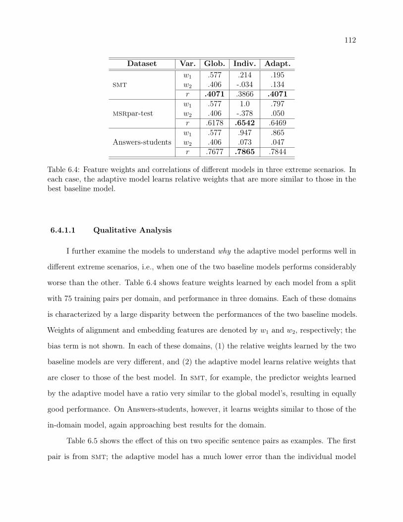
112

Dataset Var. Glob. Indiv. Adapt.

smtw1 .577 .214 .195w2 .406 -.034 .134r .4071 .3866 .4071

msrpar-testw1 .577 1.0 .797w2 .406 -.378 .050r .6178 .6542 .6469

Answers-studentsw1 .577 .947 .865w2 .406 .073 .047r .7677 .7865 .7844

Table 6.4: Feature weights and correlations of different models in three extreme scenarios. Ineach case, the adaptive model learns relative weights that are more similar to those in thebest baseline model.

6.4.1.1 Qualitative Analysis

I further examine the models to understand why the adaptive model performs well in

different extreme scenarios, i.e., when one of the two baseline models performs considerably

worse than the other. Table 6.4 shows feature weights learned by each model from a split

with 75 training pairs per domain, and performance in three domains. Each of these domains

is characterized by a large disparity between the performances of the two baseline models.

Weights of alignment and embedding features are denoted by w1 and w2, respectively; the

bias term is not shown. In each of these domains, (1) the relative weights learned by the two

baseline models are very different, and (2) the adaptive model learns relative weights that

are closer to those of the best model. In smt, for example, the predictor weights learned

by the adaptive model have a ratio very similar to the global model’s, resulting in equally

good performance. On Answers-students, however, it learns weights similar to those of the

in-domain model, again approaching best results for the domain.

Table 6.5 shows the effect of this on two specific sentence pairs as examples. The first

pair is from smt; the adaptive model has a much lower error than the individual model

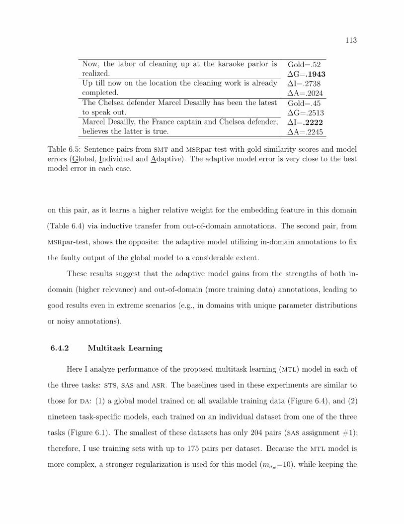
113

Now, the labor of cleaning up at the karaoke parlor isrealized.

Gold=.52∆G=.1943∆I=.2738∆A=.2024

Up till now on the location the cleaning work is alreadycompleted.The Chelsea defender Marcel Desailly has been the latestto speak out.

Gold=.45∆G=.2513∆I=.2222∆A=.2245

Marcel Desailly, the France captain and Chelsea defender,believes the latter is true.

Table 6.5: Sentence pairs from smt and msrpar-test with gold similarity scores and modelerrors (Global, Individual and Adaptive). The adaptive model error is very close to the bestmodel error in each case.

on this pair, as it learns a higher relative weight for the embedding feature in this domain

(Table 6.4) via inductive transfer from out-of-domain annotations. The second pair, from

msrpar-test, shows the opposite: the adaptive model utilizing in-domain annotations to fix

the faulty output of the global model to a considerable extent.

These results suggest that the adaptive model gains from the strengths of both in-

domain (higher relevance) and out-of-domain (more training data) annotations, leading to

good results even in extreme scenarios (e.g., in domains with unique parameter distributions

or noisy annotations).

6.4.2 Multitask Learning

Here I analyze performance of the proposed multitask learning (mtl) model in each of

the three tasks: sts, sas and asr. The baselines used in these experiments are similar to

those for da: (1) a global model trained on all available training data (Figure 6.4), and (2)

nineteen task-specific models, each trained on an individual dataset from one of the three

tasks (Figure 6.1). The smallest of these datasets has only 204 pairs (sas assignment #1);

therefore, I use training sets with up to 175 pairs per dataset. Because the mtl model is

more complex, a stronger regularization is used for this model (mσw=10), while keeping the

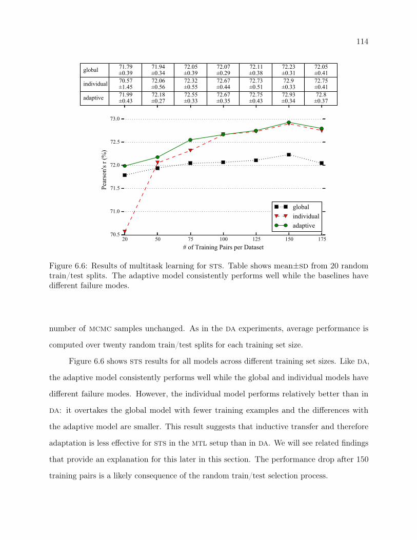
114

global 71.79±0.39

71.94±0.34

72.05±0.39

72.07±0.29

72.11±0.38

72.23±0.31

72.05±0.41

individual 70.57±1.45

72.06±0.56

72.32±0.55

72.67±0.44

72.73±0.51

72.9±0.33

72.75±0.41

adaptive 71.99±0.43

72.18±0.27

72.55±0.33

72.67±0.35

72.75±0.43

72.93±0.34

72.8±0.37

20 50 75 100 125 150 175# of Training Pairs per Dataset

70.5

71.0

71.5

72.0

72.5

73.0

Pear

son'

s r (%

)

globalindividualadaptive

Figure 6.6: Results of multitask learning for sts. Table shows mean±sd from 20 randomtrain/test splits. The adaptive model consistently performs well while the baselines havedifferent failure modes.

number of mcmc samples unchanged. As in the da experiments, average performance is

computed over twenty random train/test splits for each training set size.

Figure 6.6 shows sts results for all models across different training set sizes. Like da,

the adaptive model consistently performs well while the global and individual models have

different failure modes. However, the individual model performs relatively better than in

da: it overtakes the global model with fewer training examples and the differences with

the adaptive model are smaller. This result suggests that inductive transfer and therefore

adaptation is less effective for sts in the mtl setup than in da. We will see related findings

that provide an explanation for this later in this section. The performance drop after 150

training pairs is a likely consequence of the random train/test selection process.

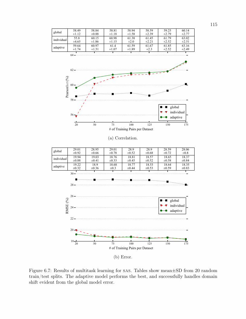
115global 58.49

±1.1258.84±0.88

58.81±1.18

58.94±1.58

58.59±2.39

59.25±2.79

60.14±2.77

individual 55.8±4.65

60.15±1.86

60.98±1.15

61.38±2.0

61.45±2.21

61.79±2.52

63.02±2.51

adaptive 59.64±1.74

60.97±1.51

61.4±1.07

61.59±1.89

61.67±2.3

61.85±2.52

63.16±2.49

20 50 75 100 125 150 175# of Training Pairs per Dataset

56

58

60

62

64

Pear

son'

s r (%

)

globalindividualadaptive

(a) Correlation.

global 29.01±0.92

28.95±0.66

29.01±0.78

28.9±0.52

28.9±0.68

28.59±0.72

28.06±0.8

individual 19.94±0.88

19.03±0.41

18.76±0.33

18.81±0.45

18.57±0.52

18.65±0.58

18.37±0.84

adaptive 19.22±0.32

18.9±0.36

18.68±0.3

18.77±0.44

18.53±0.53

18.64±0.59

18.35±0.83

20 50 75 100 125 150 175# of Training Pairs per Dataset

18

20

22

24

26

28

30

RM

SE (%

)

globalindividualadaptive

(b) Error.

Figure 6.7: Results of multitask learning for sas. Tables show mean±SD from 20 randomtrain/test splits. The adaptive model performs the best, and successfully handles domainshift evident from the global model error.

116global 75.86

±0.3976.16±0.8

76.32±0.96

76.3±1.31

75.95±1.22

76.78±1.24

76.41±1.31

individual 70.0±1.45

74.53±1.3

75.15±1.25

75.66±1.27

75.13±1.11

76.21±1.2

75.76±1.17

adaptive 75.39±1.14

75.95±0.8

76.0±1.07

76.04±1.21

75.47±1.0

76.35±1.26

76.21±1.23

20 50 75 100 125 150 175# of Training Pairs per Dataset

70

71

72

73

74

75

76

77

Mea

n A

vera

ge P

reci

sion

(%)

globalindividualadaptive

(a) Mean Average Precision.

global 82.82±0.63

82.95±0.91

83.23±1.15

82.78±1.59

82.18±1.43

83.1±1.3

82.27±1.48

individual 76.61±4.56

81.23±1.64

81.91±1.57

82.03±1.44

81.36±1.37

82.34±1.24

81.66±1.72

adaptive 82.31±1.36

82.71±0.86

82.72±1.23

82.44±1.39

81.66±1.26

82.56±1.42

82.07±1.67

20 50 75 100 125 150 175# of Training Pairs per Dataset

76

77

78

79

80

81

82

83

84

Mea

n R

ecip

roca

l Ran

k (%

)

globalindividualadaptive

(b) Mean Reciprocal Rank.

Figure 6.8: Results of multitask learning for asr. Tables show mean±SD from 20 randomtrain/test splits. Least affected by coarse-grained in-domain annotations, the global modelperforms the best; the adaptive model stays close across all training set sizes.

117

For sas, the adaptive model again has the best overall performance for both correlation

and error (Figure 6.7). The correlation plot is qualitatively similar to the sts plot, but the

global model has a much higher rmse across all training set sizes, indicating a parameter

shift across tasks. Importantly, the adaptive model remains unaffected by this shift.

The asr results in Figure 6.8 show a different pattern. Contrary to all results thus

far, the global model performs the best in this task. The individual model consistently has

lower scores, regardless of the amount of training data. Importantly, the adaptive model

stays close to the global model even with very few training examples. The asr datasets are

heavily biased towards negative examples; thus, I use stratified sampling to ensure each asr

training set has balanced examples.

A reason for the global model’s superior performance in asr may lie in the finer

granularity of the real-valued sts and sas scores compared to binary asr annotations. If a

fine granularity is indeed desirable in training data, as a model that (1) ignores in-domain

and out-of-domain distinction, and (2) utilizes a much greater number of out-of-domain

examples than in-domain ones, the global model would be affected the least by coarse-grained

asr annotations. On the other hand, the individual (i.e. domain-specific) models would be

affected the most as they are trained only on in-domain data. To test this hypothesis, I train

a linear model on all sts examples from SemEval 2012–2015 and apply it to the asr test

set via a logistic transformation. This model indeed demonstrates better results (map=.766,

mrr=.839) than the base model trained on asr annotations (Table 6.2). This is an unusual

scenario where in-domain training examples are of lower utility than out-of-domain ones,

hurting domain-specific and adaptive models.

Going back to sts, this finding also offers an explanation of why adaptation might have

been less useful in multitask learning than in domain adaptation, as only the former has asr

annotations.

118

6.5 Discussion and Related Work

The above results show that domain adaptation improves average performance across

different domains, tasks, and training set sizes. The adaptive model is also by far the least

affected by adverse factors such as noisy training data and scarcity or coarse granularity of

in-domain examples. This combination of excellent average-case and very reliable worst-case

performance makes it the model of choice for new sts domains and applications.

Although sts is a useful task with sparse data, few domain adaptation studies have

been reported. Among those is the supervised model of Heilman and Madnani [44, 45] based

on the multilevel model of Daumé III [26]. Gella et al. [38] report using a two-level stacked

regressor, where the second level combines predictions from n level 1 models, each trained on

data from a separate domain. A few unsupervised models have also been reported, based on

simpler techniques such as tagging examples with their source datasets [38, 83] and computing

vocabulary similarity between source and target domains [5]. To the best of my knowledge,

this is the first systematic study of supervised da and mtl techniques for sts with detailed

comparisons with comparable non-adaptive baselines.

6.6 Conclusions and Future Work

This chapter presents supervised domain adaptation for sts. The studies reported

focus on a common practical setting: text generated from a new domain with only a small

amount of human annotations to train models on. The hierarchical Bayesian models examined

show better overall performance over non-adaptive baselines across (1) different domains and

tasks, and (2) various amounts of training data used. Further exploration of adaptation to

other sts applications and with additional sts features (e.g., word and character n-gram

overlap) is needed to properly assess the practical utility of such techniques. Unsupervised

and semi-supervised domain adaptation techniques that do not assume the availability of

in-domain annotations provide another important avenue for future research.

Chapter 7

Conclusions

The research presented in this dissertation has focused on an important problem in

contemporary natural language processing: the automatic identification of short-text semantic

similarity (sts). While the studies reported advance the state of the art for sts and a set of

related tasks, it is imperative that we understand more fully the multifarious requirements of

text similarity and develop robust solutions based on that understanding. In this concluding

chapter, I summarize the research questions, major findings, and contributions of this work,

and point out its limitations, leading to the important discussion of possible future work.

7.1 Research Questions and Findings Revisited

Research Question 1. How can semantically similar concepts be identified in a given pair

of short text snippets?

• Similarities in the semantic units (words and phrases) of two text snippets can be a

key source of information for sts as well as other text comparison tasks including

paraphrase detection and textual entailment recognition. In view of this, I have first

explored the problem of monolingual alignment. Two high-performance word

aligners [88, 92] have been designed based on the simple hypothesis that semantically

related words across a text pair should have similarity in (1) their meaning, and (2)

their semantic contexts in the respective snippets. Evaluated on multiple benchmark

120

datasets, these systems represent the state of the art for monolingual alignment at

the time of this writing.

Research Question 2. How can sts algorithms be designed using alignment of related

concepts in the two input snippets?

• Semantically similar text pairs should have more semantically related (and thus

aligned) words than dissimilar pairs. This hypothesis has been operationalized in an

unsupervised sts system [89] that computes the proportion of aligned content words

in the two input snippets. On SemEval sts benchmarks, this lightweight system

performs remarkably well. It has then been used as a feature in a supervised sts

model [91]; augmented with a second feature derived from neural word embeddings,

this system outperforms all prior sts systems evaluated at SemEval.

Research Question 3. How can sts help in automatic question answering (qa)?

• Given a factoid question, answer sentence ranking is the task of ranking candidate

answer sentences so that actual answer-bearing sentences receive high ranks. Answer

extraction is the task of extracting a word or a small phrase from such candidates

which is a precise answer to the question. Using the semantic similarity features of

the supervised sts model, I have built a qa ranker that predicts answer sentence

relevance as a function of those features. Furthermore, this relevance score has

been used in conjunction with answer extraction features to construct a joint model

for ranking and extraction [94], yielding top results in multiple trec benchmark

datasets.

Research Question 4. How can sts help in automatically grading short answers in academic

tests?

• Given an expert-provided reference answer to a short-answer question, correct stu-

dent answers should be semantically similar to the reference answer. Based on this

121

hypothesis, I have developed an automatic short answer grader [95] that uses the pro-

posed sts features to compute the semantic similarity between student and reference

answers. Augmented with additional grading-specific features, the supervised grader

demonstrates top results in multiple grading datasets.

Research Question 5. How can sts algorithms adapt to requirements of different target

domains and applications?

• During real-life deployment of sts systems, the input text can come from various

domains (e.g., news headlines or tweets) and applications (e.g., answer grading

and qa). Text in different domains can have different properties, e.g., day-to-day

conversational English in forum qa versus syntactically well-formed English in

academic text. This can make supervised models trained on out-of-domain data less

effective on a new domain, training examples for which may be scarce. I have explored

supervised domain adaptation techniques that (1) train models on large amounts

of out-of-domain data in conjunction with much fewer in-domain annotations, and

(2) distinguish between the two types of annotations. Across different domains and

applications, these models demonstrate better overall performance than if the models

are trained on (1) just in-domain data, or (2) all available data with no distinctions

made between in-domain and out-of-domain examples [93].

7.2 Limitations

Although the sts features developed here have led to highly effective systems for both

semantic similarity identification and the downstream tasks of qa and answer grading, they

have some key limitations. Phrasal semantics, especially that of non-compositional phrases

(e.g., phrasal verbs, idioms), is captured by neither of the two features. The system completely

ignores function words as well, which can play an important role in short text semantics.

Addition of word vectors results in a bag-of-words model, insufficient for capturing the effects

122

of word order and syntax. Furthermore, the word vectors as well as the ppdb pairs are derived

from generic corpora, which can be inadequate in specialized domains such as scientific text.

Identification of long-distance semantic relations between words and phrases in a snippet—the

relationship between the two underlined words in “Three international jurists hired by the

United Nations are in Cambodia, looking at the evidence against the most important Khmer

Rouge leaders and assessing the feasibility of trials.”, for example—is limited by the capacity

of the dependency parser. Application of world knowledge is another open nlp problem that

is also important for sts—in recognizing the semantic similarity between “Thank you!” and

“I owe you one.”, for instance—but has not been addressed in the proposed system.

The goal of the sts study was not to do a comprehensive examination of sts, rather to

focus on a specific new approach based on a proposed algorithm for alignment and to see

how it influences sts and subsequent downstream applications. Design of robust sts systems

will require more thorough analyses of sts as a task, leading to a better understanding of

different input cases and system components.

For the two downstream tasks, although the proposed systems aim to address a set of

key subproblems, some of the adopted strategies prove to be inadequate (e.g., tf-idf based

term weighting in answer grading, and best chunk selection in answer extraction). Finally,

the form of domain adaptation I have explored assumes that some training data is available

for the target domain, which may not always hold.

7.3 Future Work

Short-text semantic similarity is a relatively new problem, providing ample opportunities

for future research. The proposed systems, for example, can benefit from the inclusion of

phrasal and stop word semantics. Coverage can be improved by combining lexical semantic

information from various other resources (e.g., WordNet [66]) and methods (e.g., lsa [29]).

Additional measures of similarity—ranging from shallow string similarity to deep semantic

measures like sentence embeddings [52, 96]—can complement the small feature set of the

123

supervised model. Existing sts systems—SemEval systems, for example—can also be a key

source of additional features.

The high utility of sts also makes it important to study its adaptation to different

domains and applications. Word and phrase representations specific to a target domain can

be learned by running word2vec or similar models on large amounts of target domain text.

Domain and application-specific term weighting can also be useful in certain scenarios. In the

absence of target domain annotations, unsupervised domain adaptation techniques [106, 112]

can help improve model performance.

Arguably the most important direction, however, is the pursuit of more powerful sts

models based on a full characterization of the problem. The proposed word alignment-

based model, for example, is simplistic despite its effectiveness: important factors such as

phrasal and stop word semantics, and various semantic relations that can exist between

non-paraphrases are not captured. Moreover, its strictly computational nature does not make

it a good explanatory model of human judgment of similarity, which is likely to be driven

more by a holistic interpretation of each input snippet. Construction of powerful semantic

representations of entire text snippets is a central but challenging subproblem that needs to

be solved for robust sts systems to exist. Neural sentence processing models hold promise

in this respect, given the richness of the multidimensional semantic representations these

models employ. The biggest challenge lies of course in learning the complex functions that

map meanings of words and phrases to entire snippets.

Bibliography

[1] Eneko Agirre, Carmen Banea, Claire Cardie, Daniel Cer, Mona Diab, Aitor Gonzalez-Agirre, Weiwei Guo, Inigo Lopez-Gazpio, Montse Maritxalar, Rada Mihalcea, GermanRigau, Larraitz Uria, and Janyce Wiebe. SemEval-2015 task 2: Semantic textualsimilarity, English, Spanish and pilot on interpretability. In Proceedings of the 9thInternational Workshop on Semantic Evaluation, SemEval ’15, Denver, Colorado, 2015.

[2] Eneko Agirre, Carmen Banea, Claire Cardie, Daniel Cer, Mona Diab, Aitor Gonzalez-Agirre, Weiwei Guo, Rada Mihalcea, German Rigau, and Janyce Wiebe. SemEval-2014task 10: Multilingual semantic textual similarity. In Proceedings of the 8th InternationalWorkshop on Semantic Evaluation, SemEval ’14, Dublin, Ireland, 2014.

[3] Eneko Agirre, Daniel Cer, Mona Diab, Aitor Gonzalez-Agirre, and Weiwei Guo. *SEM2013 shared task: Semantic textual similarity. In Second Joint Conference on Lexicaland Computational Semantics, *SEM ’13, Atlanta, Georgia, USA, 2013.

[4] Eneko Agirre, Mona Diab, Daniel Cer, and Aitor Gonzalez-Agirre. SemEval-2012 task6: A pilot on semantic textual similarity. In Proceedings of the Sixth InternationalWorkshop on Semantic Evaluation, SemEval ’12, Montréal, Canada, 2012.

[5] Piyush Arora, Chris Hokamp, Jennifer Foster, and Gareth Jones. DCU: Using distribu-tional semantics and domain adaptation for the semantic textual similarity SemEval-2015 task 2. In Proceedings of the 9th International Workshop on Semantic Evaluation,SemEval ’15, Denver, Colorado, 2015.

[6] Rajendra Banjade, Nobal Bikram Niraula, Nabin Maharjan, Vasile Rus, Dan Stefanescu,Mihai Lintean, and Dipesh Gautam. NeRoSim: A system for measuring and interpretingsemantic textual similarity. In Proceedings of the 9th International Workshop onSemantic Evaluation, SemEval ’15, Denver, Colorado, USA, 2015.

[7] Colin Bannard and Chris Callison-Burch. Paraphrasing with bilingual parallel cor-pora. In Proceedings of the 43rd Annual Meeting on Association for ComputationalLinguistics, ACL ’05, Ann Arbor, Michigan, 2005.

[8] Daniel Bär, Chris Biemann, Iryna Gurevych, and Torsten Zesch. UKP: Computingsemantic textual similarity by combining multiple content similarity measures. InProceedings of the Sixth International Workshop on Semantic Evaluation, SemEval’12, Montréal, Canada, 2012.

125

[9] Daniel Bär, Torsten Zesch, and Iryna Gurevych. Text reuse detection using a compo-sition of text similarity measures. In Proceedings of COLING 2012, Mumbai, India,2012.

[10] Marco Baroni, Georgiana Dinu, and Germán Kruszewski. Don’t count, predict! Asystematic comparison of context-counting vs. context-predicting semantic vectors.In Proceedings of the 52nd Annual Meeting of the Association for ComputationalLinguistics, ACL ’14, Baltimore, Maryland, 2014.

[11] Islam Beltagy, Katrin Erk, and Raymond Mooney. Probabilistic soft logic for semantictextual similarity. In Proceedings of the 52nd Annual Meeting of the Association forComputational Linguistics, ACL ’14, Baltimore, Maryland, 2014.

[12] Yoshua Bengio, Réjean Ducharme, Pascal Vincent, and Christian Janvin. A neuralprobabilistic language model. Journal of Machine Learning Research, 3, 2003.

[13] Daniel M. Bikel, Richard Schwartz, and Ralph M. Weischedel. An algorithm that learnswhat’s in a name. Machine Learning, 34(1-3), 1999.

[14] Steven Bird, Edward Loper, and Ewan Klein. Natural Language Processing withPython. O’Reilly Media Inc., 2009.

[15] David M. Blei, Andrew Y. Ng, and Michael I. Jordan. Latent Dirichlet allocation.Journal of Machine Learning Research, 3, 2003.

[16] Chris Brockett. Aligning the RTE 2006 corpus. Technical Report MSR-TR-2007-77,Microsoft Research, 2007.

[17] Elia Bruni, Nam Khanh Tran, and Marco Baroni. Multimodal distributional semantics.Journal of Artificial Intelligence Research, 49(1), 2014.

[18] Steven Burrows, Iryna Gurevych, and Benno Stein. The eras and trends of automaticshort answer grading. International Journal of Artificial Intelligence in Education, 25.2,2015.

[19] Yee Seng Chan and Hwee Tou Ng. MAXSIM: A maximum similarity metric for machinetranslation evaluation. In Proceedings of the 52nd Annual Meeting of the Associationfor Computational Linguistics: Human Language Technologies, ACL ’08, Columbus,Ohio, 2008.

[20] Stephen Clark. Vector space models of lexical meaning. Handbook of ContemporarySemantics, 2nd ed, 2013.

[21] Paul Clough, Robert Gaizauskas, Scott S.L. Piao, and Yorick Wilks. Measuring textreuse. In Proceedings of 40th Annual Meeting of the Association for ComputationalLinguistics, ACL ’02, Philadelphia, Pennsylvania, USA, 2002.

126

[22] Ronan Collobert and Jason Weston. A unified architecture for natural languageprocessing: Deep neural networks with multitask learning. In Proceedings of the 25thInternational Conference on Machine Learning, ICML ’08, Helsinki, Finland, 2008.

[23] Ido Dagan, Dan Roth, Mark Sammons, and Fabio Massimo Zanzotto. RecognizingTextual Entailment: Models and Applications. Synthesis Lectures on Human LanguageTechnologies. Morgan & Claypool Publishers, 2013.

[24] Dipanjan Das and Noah A. Smith. Paraphrase identification as probabilistic quasi-synchronous recognition. In Proceedings of the Joint Conference of the 47th AnnualMeeting of the ACL and the 4th International Joint Conference on Natural LanguageProcessing of the AFNLP, ACL ’09, Stroudsburg, PA, USA, 2009.

[25] Anirban Dasgupta, Ravi Kumar, and Sujith Ravi. Summarization through submod-ularity and dispersion. In Proceedings of the 51st Annual Meeting of the Associationfor Computational Linguistics, ACL ’13, Sofia, Bulgaria, 2013.

[26] Hal Daumé III. Frustratingly easy domain adaptation. In Proceedings of the 45thAnnual Meeting of the Association of Computational Linguistics, ACL ’07, Prague,Czech Republic, 2007.

[27] Marie-Catherine de Marneffe, Bill MacCartney, and Christopher D. Manning. Gen-erating typed dependency parses from phrase structure parses. In Proceedings of theInternational Conference on Language Resources and Evaluation, LREC ’06, Genoa,Italy, 2006.

[28] Marie-Catherine de Marneffe and Christopher D. Manning. Stanford typed dependenciesmanual. Technical report, Stanford University, 2008.

[29] Scott Deerwester, Susan T. Dumais, George W. Furnas, Thomas K. Landauer, andRichard Harshman. Indexing by latent semantic analysis. Journal of the AmericanSociety for Information Science, 41, 1990.

[30] Bill Dolan, Chris Quirk, and Chris Brockett. Unsupervised construction of largeparaphrase corpora: Exploiting massively parallel news sources. In Proceedings of the20th International Conference on Computational Linguistics, COLING ’04, Geneva,Switzerland, 2004.

[31] Myroslava Dzikovska, Rodney Nielsen, Chris Brew, Claudia Leacock, Danilo Giampic-colo, Luisa Bentivogli, Peter Clark, Ido Dagan, and Hoa Trang Dang. SemEval-2013task 7: The joint student response analysis and 8th recognizing textual entailment chal-lenge. In Proceedings of the Seventh International Workshop on Semantic Evaluation,SemEval ’13, Atlanta, Georgia, USA, 2013.

[32] Katrin Erk. Vector space models of word meaning and phrase meaning: A survey.Language and Linguistics Compass, 6(10), 2012.

127

[33] David A. Ferrucci, Eric W. Brown, Jennifer Chu-Carroll, James Fan, David Gondek,Aditya Kalyanpur, Adam Lally, J. William Murdock, Eric Nyberg, John M. Prager, NicoSchlaefer, and Christopher A. Welty. Building Watson: An overview of the DeepQAproject. AI Magazine, 31(3), 2010.

[34] Jenny Rose Finkel, Trond Grenager, and Christopher Manning. Incorporating non-localinformation into information extraction systems by Gibbs sampling. In Proceedingsof the 43rd Annual Meeting on Association for Computational Linguistics, ACL ’05,Ann Arbor, Michigan, USA, 2005.

[35] Jenny Rose Finkel and Christopher D. Manning. Hierarchical Bayesian domain adapta-tion. In Proceedings of Human Language Technologies: The 2009 Annual Conference ofthe North American Chapter of the Association for Computational Linguistics, NAACL’09, Boulder, Colorado, USA, 2009.

[36] Zvi Galil. Efficient algorithms for finding maximum matching in graphs. ACMComputing Surveys, 18(1), 1986.

[37] Juri Ganitkevitch, Benjamin Van Durme, and Chris Callison-Burch. PPDB: The para-phrase database. In Proceedings of the 2013 Conference of the North American Chapterof the Association for Computational Linguistics – Human Language Technologies,NAACL ’13, Atlanta, Georgia, USA, 2013.

[38] Spandana Gella, Bahar Salehi, Marco Lui, Karl Grieser, Paul Cook, and TimothyBaldwin. UniMelb_NLP-CORE: Integrating predictions from multiple domains andfeature sets for estimating semantic textual similarity. In Proceedings of the SecondJoint Conference on Lexical and Computational Semantics, *SEM ’13, Atlanta, Georgia,USA, 2013.

[39] Danilo Giampiccolo, Bernardo Magnini, Ido Dagan, and Bill Dolan. The third PAS-CAL recognizing textual entailment challenge. In Proceedings of the ACL-PASCALWorkshop on Textual Entailment and Paraphrasing, RTE ’07, Prague, Czech Republic,2007.

[40] Daniel Gildea and Daniel Jurafsky. Automatic labeling of semantic roles. ComputationalLinguistics, 28(3), 2002.

[41] Guy Halawi, Gideon Dror, Evgeniy Gabrilovich, and Yehuda Koren. Large-scalelearning of word relatedness with constraints. In Proceedings of the 18th ACM SIGKDDInternational Conference on Knowledge Discovery and Data Mining, KDD ’12, Beijing,China, 2012.

[42] Lushan Han, Abhay L. Kashyap, Tim Finin, James Mayfield, and Jonathan Weese.UMBC_EBIQUITY-CORE: Semantic textual similarity systems. In Second JointConference on Lexical and Computational Semantics, *SEM ’13, Atlanta, Georgia,USA, 2013.

128

[43] Christian Hänig, Robert Remus, and Xose de la Puente. ExB Themis: Extensive featureextraction from word alignments for semantic textual similarity. In Proceedings of the9th International Workshop on Semantic Evaluation, SemEval ’15, Denver, Colorado,USA, 2015.

[44] Michael Heilman and Nitin Madnani. ETS: Domain adaptation and stacking for shortanswer scoring. In Proceedings of the Seventh International Workshop on SemanticEvaluation, SemEval ’13, Atlanta, Georgia, USA, 2013.

[45] Michael Heilman and Nitin Madnani. HENRY-CORE: Domain adaptation and stackingfor text similarity. In Proceedings of the Second Joint Conference on Lexical andComputational Semantics, *SEM ’13, Atlanta, Georgia, USA, 2013.

[46] Michael Heilman and Noah A. Smith. Tree edit models for recognizing textual entail-ments, paraphrases, and answers to questions. In Proceedings of the 2010 Conferenceof the North American Chapter of the Association for Computational Linguistics –Human Language Technologies, NAACL ’10, Los Angeles, California, USA, 2010.

[47] Andrew Hickl and Jeremy Bensley. A discourse commitment-based framework forrecognizing textual entailment. In Proceedings of the ACL-PASCAL Workshop onTextual Entailment and Paraphrasing, RTE ’07, Prague, Czech Republic, 2007.

[48] Aminul Islam and Diana Inkpen. Semantic text similarity using corpus-based wordsimilarity and string similarity. ACM Transactions on Knowledge Discovery from Data,2(2), 2008.

[49] Sergio Jimenez, Claudia Becerra, and Alexander Gelbukh. Soft Cardinality: A parame-terized similarity function for text comparison. In Proceedings of the Sixth InternationalWorkshop on Semantic Evaluation, SemEval ’12, Montréal, Canada, 2012.

[50] Sergio Jimenez, Claudia Becerra, and Alexander Gelbukh. SOFTCARDINALITY-CORE: Improving text overlap with distributional measures for semantic textual simi-larity. In Second Joint Conference on Lexical and Computational Semantics (*SEM),*SEM ’13, Atlanta, Georgia, USA, 2013.

[51] Sergio Jimenez, Claudia Becerra, and Alexander Gelbukh. SOFTCARDINALITY:Hierarchical text overlap for student response analysis. In Proceedings of the SeventhInternational Workshop on Semantic Evaluation, SemEval ’13, Atlanta, Georgia, USA,2013.

[52] Nal Kalchbrenner and Phil Blunsom. Recurrent continuous translation models.In Proceedings of the 2013 Conference on Empirical Methods in Natural LanguageProcessing, EMNLP ’13, Seattle, Washington, USA, 2013.

[53] Peter Kolb. DISCO: A multilingual database of distributionally similar words. InProceedings of the 9th Conference on Natural Language Processing, KONVENS ’08,Berlin, Germany, 2008.

129

[54] Adam Lally, John M. Prager, Michael C. McCord, Branimir K. Boguraev, SiddharthPatwardhan, Paul Fodor James Fan, and Jennifer Chu-Carroll. Question analysis: HowWatson reads a clue. IBM Journal of Research and Development, 56(3.4), 2012.

[55] Claudia Leacock and Martin Chodorow. C-rater: Automated scoring of short-answerquestions. Computers and the Humanities, 37(04), 2003.

[56] Yuhua Li, David McLean, Zuhair A. Bandar, James D. O’Shea, and Keeley Crockett.Sentence similarity based on semantic nets and corpus statistics. IEEE Transactionson Knowledge and Data Engineering, 18(8), 2006.

[57] Jimmy Lin and Boris Katz. Building a reusable test collection for question answering.Journal of the American Society for Information Science and Technology, 57(7), 2006.

[58] Chang Liu, Daniel Dahlmeier, and Hwee Tou Ng. Better evaluation metrics lead tobetter machine translation. In Proceedings of the Conference on Empirical Methodsin Natural Language Processing, EMNLP ’11, Edinburgh, UK, 2011.

[59] André Lynum, Partha Pakray, Björn Gambäck, and Sergio Jimenez. NTNU: Measuringsemantic similarity with sublexical feature representations and soft cardinality. InProceedings of the 8th International Workshop on Semantic Evaluation, SemEval ’14,Dublin, Ireland, 2014.

[60] Bill MacCartney, Michel Galley, and Christopher D. Manning. A phrase-based alignmentmodel for natural language inference. In Proceedings of the Conference on EmpiricalMethods in Natural Language Processing, EMNLP ’08, Honolulu, Hawaii, 2008.

[61] Nitin Madnani, Joel Tetreault, and Martin Chodorow. Re-examining machine transla-tion metrics for paraphrase identification. In Proceedings of the 2012 Conference of theNorth American Chapter of the Association for Computational Linguistics: HumanLanguage Technologies, NAACL ’12, Montreal, Canada, 2012.

[62] Erwin Marsi, Hans Moen, Lars Bungum, Gleb Sizov, Björn Gambäck, and AndréLynum. NTNU-CORE: Combining strong features for semantic similarity. In SecondJoint Conference on Lexical and Computational Semantic, *SEM ’13, Atlanta, Georgia,USA, 2013.

[63] Ryan McDonald, Koby Crammer, and Fernando Pereira. Online large-margin trainingof dependency parsers. In Proceedings of the 43rd Annual Meeting of the Associationfor Computational Linguistics, ACL ’05, Ann Arbor, Michigan, 2005.

[64] Rada Mihalcea, Courtney Corley, and Carlo Strapparava. Corpus-based and knowledge-based measures of text semantic similarity. In Proceedings of the 21st NationalConference on Artificial Intelligence, AAAI ’06, 2006.

[65] Tomas Mikolov, Kai Chen, Greg Corrado, and Jeffrey Dean. Efficient estimation ofword representations in vector space. In Proceedings of the International Conferenceon Learning Representations Workshop, Scottsdale, Arizona, USA, 2013.

130

[66] George A. Miller. WordNet: A lexical database for English. Communications of theACM, 38(11), November 1995.

[67] Tom Mitchell, Terry Russell, Peter Broomhead, and Nicola Aldridge. Towards robustcomputerised marking of free-text responses. In Proceedings of the 6th InternationalComputer Assisted Assessment Conference, CAA ’02, Loughborough, UK, 2002.

[68] Michael Mohler, Razvan Bunescu, and Rada Mihalcea. Learning to grade shortanswer questions using semantic similarity measures and dependency graph alignments.In Proceedings of the 49th Annual Meeting of the Association for ComputationalLinguistics: Human Language Technologies, ACL ’11, Portland, Oregon, USA, 2011.

[69] Michael Mohler and Rada Mihalcea. Text-to-text semantic similarity for automaticshort answer grading. In Proceedings of the 12th Conference of the European Chapterof the ACL, EACL ’09, Athens, Greece, 2009.

[70] Daniel Myers and James W. McGuffee. Choosing Scrapy. Computing Sciences inColleges, 31(1), 2015.

[71] Rodney D. Nielsen, Wayne Ward, and James H. Martin. Recognizing entailment inintelligent tutoring systems. Natural Language Engineering, 15(04), 2009.

[72] Martha Palmer, Daniel Gildea, and Paul Kingsbury. The Proposition Bank: Anannotated corpus of semantic roles. Computational Linguistics, 31(1), 2005.

[73] Anand Patil, David Huard, and Christopher J. Fonnesbeck. PyMC: Bayesian stochasticmodelling in Python. Journal of Statistical Software, 35(4), 2010.

[74] Fabian Pedregosa, Gaël Varoquaux, Alexandre Gramfort, Vincent Michel, BertrandThirion, Olivier Grisel, Mathieu Blondel, Peter Prettenhofer, Ron Weiss, VincentDubourg, Jake Vanderplas, Alexandre Passos, David Cournapeau, Matthieu Brucher,Matthieu Perrot, and Édouard Duchesnay. Scikit-learn: Machine learning in Python.Journal of Machine Learning Research, 12, 2011.

[75] Mohammad Taher Pilehvar, David Jurgens, and Roberto Navigli. Align, disambiguateand walk: a unified approach for measuring semantic similarity. In Proceedings of the51st Annual Meeting of the Association for Computational Linguistics, ACL ’13, Sofia,Bulgaria, 2013.

[76] Kira Radinsky, Eugene Agichtein, Evgeniy Gabrilovich, and Shaul Markovitch. Aword at a time: Computing word relatedness using temporal semantic analysis. InProceedings of the 20th International Conference on World Wide Web, WWW ’11,Hyderabad, India, 2011.

[77] Lakshmi Ramachandran, Jian Cheng, and Peter Foltz. Identifying patterns for shortanswer scoring using graph-based lexico-semantic text matching. In Proceedings ofthe Tenth Workshop on Innovative Use of NLP for Building Educational Applications,NAACL-BEA ’15, 2015.

131

[78] Adwait Ratnaparkhi. A maximum entropy model for part-of-speech tagging. InProceedings of the 1996 Conference on Empirical Methods in Natural LanguageProcessing, EMNLP ’96, Philadelphia, Pennsylvania, USA, 1996.

[79] G. Salton and M. E. Lesk. Computer evaluation of indexing and text processing.Journal of the ACM, 15(1), January 1968.

[80] John Salvatier, Thomas V. Wiecki, and Christopher Fonnesbeck. Probabilistic pro-gramming in Python using PyMC. arXiv:1507.08050v1, 2015.

[81] Aliaksei Severyn and Alessandro Moschitti. Automatic feature engineering for answerselection and extraction. In Proceedings of the 2013 Conference on Empirical Methodsin Natural Language Processing, EMNLP ’13, Seattle, Washington, USA, 2013.

[82] Aliaksei Severyn and Alessandro Moschitti. Learning to rank short text pairs withconvolutional deep neural networks. In Proceedings of the 38th International ACMSIGIR Conference on Research and Development in Information Retrieval, SIGIR ’15,Santiago, Chile, 2015.

[83] Aliaksei Severyn, Massimo Nicosia, and Alessandro Moschitti. Learning semantictextual similarity with structural representations. In Proceedings of the 51st AnnualMeeting of the Association for Computational Linguistics, ACL ’13, 2013.

[84] Ehsan Shareghi and Sabine Bergler. CLaC-CORE: Exhaustive feature combination formeasuring textual similarity. In Second Joint Conference on Lexical and ComputationalSemantics, *SEM ’13, Atlanta, Georgia, USA, 2013.

[85] Eyal Shnarch. Probabilistic Models for Lexical Inference. PhD thesis, Bar Ilan Univer-sity, 2013.

[86] Richard Socher, Eric H. Huang, Jeffrey Pennington, Andrew Y. Ng, and Christopher D.Manning. Dynamic pooling and unfolding recursive autoencoders for paraphrasedetection. In Advances in Neural Information Processing Systems, NIPS ’11, 2011.

[87] Jana Z. Sukkarieh, Stephen G. Pulman, and Nicholas Raikes. Auto-Marking 2: Anupdate on the UCLES-Oxford University research into using computational linguisticsto score short, free text responses. In Proceedings of the 30th Annual Conference ofthe International Association for Educational Assessment, Philadelphia, Pennsylvania,USA, 2004.

[88] Md Arafat Sultan, Steven Bethard, and Tamara Sumner. Back to basics for monolingualalignment: Exploiting word similarity and contextual evidence. Transactions of theAssociation for Computational Linguistics, 2, 2014.

[89] Md Arafat Sultan, Steven Bethard, and Tamara Sumner. DLS@CU: Sentence similarityfrom word alignment. In Proceedings of the 8th International Workshop on SemanticEvaluation, SemEval ’14, Dublin, Ireland, 2014.

132

[90] Md Arafat Sultan, Steven Bethard, and Tamara Sumner. Towards automatic iden-tification of core concepts in educational resources. In Proceedings of the 14thACM/IEEE-CS Joint Conference on Digital Libraries, JCDL ’14, London, UnitedKingdom, 2014.

[91] Md Arafat Sultan, Steven Bethard, and Tamara Sumner. DLS@CU: Sentence similarityfrom word alignment and semantic vector composition. In Proceedings of the 9thInternational Workshop on Semantic Evaluation, SemEval ’15, Denver, Colorado, USA,2015.

[92] Md Arafat Sultan, Steven Bethard, and Tamara Sumner. Feature-rich two-stagelogistic regression for monolingual alignment. In Proceedings of the 2015 Conferenceon Empirical Methods in Natural Language Processing, EMNLP ’15, Lisbon, Portugal,2015.

[93] Md Arafat Sultan, Jordan Boyd-Graber, and Tamara Sumner. Bayesian superviseddomain adaptation for short text similarity. In Proceedings of the 2016 Conferenceof the North American Chapter of the Association for Computational Linguistics –Human Language Technologies, NAACL ’16, San Diego, California, USA, 2016.

[94] Md Arafat Sultan, Vittorio Castelli, and Radu Florian. A joint model for answer sentenceranking and answer extraction. Transactions of the Association for ComputationalLinguistics, 2016.

[95] Md Arafat Sultan, Cristobal Salazar, and Tamara Sumner. Fast and easy shortanswer grading with high accuracy. In Proceedings of the 2016 Conference of theNorth American Chapter of the Association for Computational Linguistics – HumanLanguage Technologies, NAACL ’16, San Diego, California, USA, 2016.

[96] Ilya Sutskever, Oriol Vinyals, and Quoc V Le. Sequence to sequence learning withneural networks. In Advances in Neural Information Processing Systems 27, NIPS ’14,Montréal, Canada, 2014.

[97] Louis Tandalla. Scoring short answer essays. https://kaggle2.blob.core.windows.net/competitions/kaggle/2959/media/TechnicalMethodsPaper.pdf.

[98] Kapil Thadani, Scott Martin, and Michael White. A joint phrasal and dependencymodel for paraphrase alignment. In Proceedings of the 24th International Conferenceon Computational Linguistics: Posters, COLING ’12, Mumbai, India, 2012.

[99] Kapil Thadani and Kathleen McKeown. Optimal and syntactically-informed decodingfor monolingual phrase-based alignment. In Proceedings of the 49th Annual Meeting ofthe Association for Computational Linguistics: Human Language Technologies, ACL’11, Portland, Oregon, USA, 2011.

[100] Kristina Toutanova, Dan Klein, Christopher D. Manning, and Yoram Singer. Feature-rich part-of-speech tagging with a cyclic dependency network. In Proceedings of the

133

2003 Conference of the North American Chapter of the Association for ComputationalLinguistics – Human Language Technologies, NAACL ’03, Edmonton, Canada, 2003.

[101] Frane Šarić, Goran Glavaš, Mladen Karan, Jan Šnajder, and Bojana Dalbelo Bašić.TakeLab: Systems for measuring semantic text similarity. In Proceedings of the SixthInternational Workshop on Semantic Evaluation, SemEval ’12, Montréal, Canada, 2012.

[102] Lu Wang, Hema Raghavan, Vittorio Castelli, Radu Florian, and Claire Cardie. Asentence compression based framework to query-focused multi-document summariza-tion. In Proceedings of the 51st Annual Meeting of the Association for ComputationalLinguistics, ACL ’13, Sofia, Bulgaria, 2013.

[103] Mengqiu Wang and Christopher Manning. Probabilistic tree-edit models with structuredlatent variables for textual entailment and question answering. In Proceedings of the23rd International Conference on Computational Linguistics, Coling ’10, Beijing, China,2010.

[104] Mengqiu Wang, Noah A. Smith, and Teruko Mitamura. What is the Jeopardy model?A quasi-synchronous grammar for QA. In Proceedings of the 2007 Conference onEmpirical Methods in Natural Language Processing, EMNLP ’07, 2007.

[105] Stephen Wu, Dongqing Zhu, Ben Carterette, and Hongfang Liu. MayoClinicNLP-CORE:Semantic representations for textual similarity. In Proceedings of the Second JointConference on Lexical and Computational Semantics, *SEM ’13, Atlanta, Georgia,USA, 2013.

[106] Yi Yang and Jacob Eisenstein. Unsupervised multi-domain adaptation with feature em-beddings. In Proceedings of the 2015 Conference of the North American Chapter of theAssociation for Computational Linguistics: Human Language Technologies, NAACL’15, Denver, Colorado, 2015.

[107] Xuchen Yao, Benjamin Van Durme, Chris Callison-Burch, and Peter Clark. An-swer extraction as sequence tagging with tree edit distance. In Proceedings of the2013 Conference of the North American Chapter of the Association for ComputationalLinguistics – Human Language Technologies, NAACL ’13, Atlanta, Georgia, USA,2013.

[108] Xuchen Yao, Benjamin Van Durme, Chris Callison-Burch, and Peter Clark. A lightweightand high performance monolingual word aligner. In Proceedings of the 51st AnnualMeeting of the Association for Computational Linguistics, ACL ’13, Sofia, Bulgaria,2013.

[109] Xuchen Yao, Benjamin Van Durme, Chris Callison-Burch, and Peter Clark. Semi-Markov phrase-based monolingual alignment. In Proceedings of the 2013 Conference onEmpirical Methods in Natural Language Processing, EMNLP ’13, Seattle, Washington,USA, 2013.

134

[110] Xuchen Yao, Benjamin Van Durme, and Peter Clark. Automatic coupling of answerextraction and information retrieval. In Proceedings of the 51st Annual Meeting of theAssociation for Computational Linguistics, ACL ’13, Sofia, Bulgaria, 2013.

[111] Wen-tau Yih, Ming-Wei Chang, Christopher Meek, and Andrzej Pastusiak. Questionanswering using enhanced lexical semantic models. In Proceedings of the 51st AnnualMeeting of the Association for Computational Linguistics, ACL ’13, Sofia, Bulgaria,2013.

[112] Jianfei Yu and Jing Jiang. A hassle-free unsupervised domain adaptation methodusing instance similarity features. In Proceedings of the 53rd Annual Meeting of theAssociation for Computational Linguistics and the 7th International Joint Conferenceon Natural Language Processing, ACL-IJCNLP ’15, Beijing, China, 2015.

[113] Lei Yu, Karl Moritz Hermann, Phil Blunsom, and Stephen Pulman. Deep learning foranswer sentence selection. In NIPS Deep Learning Workshop, 2014.