Short term power forecasts for large offshore wind turbine

Short term power forecasts for large offshore wind turbine arrays ESGI91

Short term power forecasts for large offshore

wind turbine arrays

Problem presented by

Jeremy Parkes

GL Garad Hassan

Executive Summary

Methods are presented for precise prediction of windspeeds at a wind-

farm using a combination of numerical weather prediction models and

on-site wind speed measurements. Simple techniques are used to inves-

tigate the properties of the data. More advanced techniques are tested

for the predictive value in forecasting including techniques from autore-

gressive models, data assimilation, artificial neural networks and kernel

dressing. The performance of the resulting forecasts are compared with

the measured wind speeds using a range of forecast windows.

Version 1.0

October 24, 2013

iii+26 pages

i


Report author

Oscar Benjamin, Petros Mina, Laszlo Arany, Colm Connaughton, Sam Cox,

Milena Kresoja, Abhishek Shukla, Ed Wheatcroft, James Tull, Samuel Groth,

Sian Jenkins, Chris Budd, Leonard Smith

Contributors

Oscar Benjamin (University of Bristol),

Petros Mina (University of Bristol),

Laszlo Arany (University of Bristol),

Colm Connaughton (University of Warwick),

Sam Cox (University of Leicester),

Milena Kresoja (University of Novi Sad),

Abhishek Shukla (University of Warwick),

Ed Wheatcroft (London School of Economics),

James Tull (Imperial College),

Samuel Groth (University of Reading),

Sian Jenkins (University of Bath),

Chris Budd (University of Bath),

Leonard Smith (London School of Economics)

ESGI91 was jointly organised by

University of Bristol

Knowledge Transfer Network for Industrial Mathematics

and was supported by

Natural Environment Research Council

Oxford Centre for Collaborative Applied Mathematics

Warwick Complexity Centre

ii


Contents

1 Introduction 1

2 Instantaneous linear prediction 4

3 Auto-regressive models 6

4 4D-Var Data assimilation 10

5 Artificial neural networks 15

5.1 Generalised Regression Neural Networks . . . . . . . . . . . . . . . 15

5.2 ANN prediction from SCADA data . . . . . . . . . . . . . . . . . . 16

5.3 ANN prediction from Numerical Weather Prediction data . . . . . . 18

5.4 Remarks and possible future work . . . . . . . . . . . . . . . . . . . 19

6 Kernel dressing 20

6.1 Running mean and variance normal distribution model . . . . . . . 23

6.2 Individual Kernel Dressed Model forecasts . . . . . . . . . . . . . . 24

6.3 Possible future work . . . . . . . . . . . . . . . . . . . . . . . . . . 25

7 Conclusions 25

Bibliography 26

iii


1 Introduction

(1.1) Onshore and offshore windfarms are increasingly being used for power gener-

ation both in the UK and globally. Since power generation from windfarms

is intermittent, a reliable electricity supply must use windfarms in combi-

nations with other energy sources. It is only possible to make use of the

energy from windfarms by producing less energy from other energy sources

if the output can be reliably predicted in advance. Since the most signifi-

cant factor determining the power generation of a windfarm is wind speed

accurate forecasts of this are essential. However, wind speed can change

dramatically on a timescale of hours. Figure 1 shows recordings of wind

speeds from an offshore windfarm.

Figure 1: Measured wind speeds at an offshore windfarm at differenttimescales. The top panel shows wind speed measurements over a wholeyear. The bottom panel shows wind speed measurements over the firstweek of the year. The long straight line from 1st-2nd Jan is a periodduring which no measurement data is available.

(1.2) GL Garrad Hassan (GH) provides a continuous real-time forecasting service

to operators of windfarms providing accurate predictions of wind speed and

1


power output for individual windfarms from 0-48 hours in advance. The

forecasting service makes predictions based on numerical weather predic-

tion (NWP) models and onsite wind measurements (known as SCADA).

The NWP and SCADA data are combined to produce estimates of future

windspeed with a root mean squared (RMS) error ranging from around 2%

(1 hour in advance) to around 6% (48 hours in advance).

(1.3) NWP models are macroscale numerical simulations of atmospheric dynam-

ics used for weather forecasting in general. Different NWP models are more

accurate for predicting the weather under different situations. Forecasters

using NWP models will release predictions of the weather for up to two

weeks in advance and update their prediction every 3-12 hours. Each fore-

cast gives a prediction of the weather for each hour over the subsequent 1-2

weeks. NWP models describe the atmosphere in terms of finite elements

where the size of each element is on the order of kilometres. GH uses in-

terpolation to convert this to an estimate of the weather at the site of the

windfarm. Figure 2 shows how the forecast estimate at different times in

advance correlates with the recorded windspeed for different NWP models

for a specific windfarm. The correlation for the NWP models ranges from

around 0.9 for forecasting (or estimating) the windspeed at the current time

to around 0.7-0.8 for forecasting 48 hours ahead.

(1.4) SCADA data recording the actual windspeed at windfarms is available to

GH in real time. Every 10 minutes an average wind speed and direction

measurement is received by GH. This reading is based on the previous 10

minutes before the measurement is received. This data is used both to make

a forecast and also to validate forecasts retrospectively. Figure 2 shows that

the correlation between the SCADA windspeed data and its own value at

a later time is higher when compared to the correlation between the NWP

forecast and the actual wind speed over a 0-3 hours window. This suggests

that at very short times the best prediction of the windspeed should be

based strongly on the SCADA data. However, when forecasting more than

10 hours ahead the SCADA data has a much lower correlation than any of

the NWP models, so the NWP data will likely have more predictive value

in this window.

(1.5) GH combines the NWP and SCADA data to provide realtime forecasting.

2


0 10 20 30 400.1

0.2

0.3

0.4

0.5

0.6

0.7

0.8

0.9

1

prediction time window (hrs)

corr

elat

ion

coef

ficie

nt

corellation coeffients of NWPs as function of forecast time

0 10 20 30 400.7

0.75

0.8

0.85

0.9

0.95

1

prediction time window (hrs)

corr

elat

ion

coef

ficie

nt

NWP1NWP2NWP3NWP4SCADA

Figure 2: Correlation between NWP estimates of the wind speed andNWP predictions as a function of prediction time window. The predic-tion time window is the the number of hours in advance that a forecastis made for the wind speed. For this windfarm there are 4 differentNWP models available giving different predictions. Also shown is theautocorrelation of the measured windspeeds (SCADA). The panel onthe right shows a zoom view of the panel on the left to better illustratethe differences between the NWP models. The SCADA data gives ahigher correlation for time windows less than 2 hours but correlates sig-nificantly less well than all of the NWP predictions at windows of morethan around 4 hours.

They have combined a number of techniques for extracting an improved fore-

cast of weather at the site of the windfarm based on the NWP and SCADA

data available. The aim of the study group was to investigate the scope

for using novel techniques not employed by GH in the area of windspeed

prediction. The study group has investigated the data, applied a number

of different techniques for combining the data sources, and attempted to

evalute their applicability. In the following sections each method and the

available results are described, starting with the simplest that we use as

3


benchmarks.

2 Instantaneous linear prediction

(2.1) Linear regression analysis is perhaps the most simple form of bias correc-

tion. The aim is to eradicate some of the systematic error in the different

forecasts by first assuming (slightly naıvely) that the error in the windspeed

forecast is linear. This systematic error can be seen in figure 3. Each of the

NWP models obtains approximately the correct distribution of windspeeds

throughout the year when compared with the measured data, however they

are all approximately shifted somewhat.

Figure 3: Forecast windspeed by the 4 different NWP models oneday in advance compared with the on-site measured winspeeds for alldays (for which there is data) in 2012. For visual clarity the days (x-axis) have been reordered to produce a plot where the windspeed ismonotonically increasing.

(2.2) We can calculate the shift by simply computing the least squares fit of

each NWP output to the measured data. The shifted NWPs are shown in

figure 4. The process of least squares fitting will be elaborated upon below.

(2.3) A slightly different approach is to combine the four different forecasts in

such a way as to obtain a forecast superior to each of the individual NWP

models. This is done by taking a linear combiniation of the output of the

four NWPs, that is, we write:

ÑWP = w1NWP1 + w2NWP2 + w3NWP3 + w4NWP4. (2.1)

4


Figure 4: Forecast windspeed of the 4 different NWP models presentedin figure 3 after the bias is corrected for, alongside on-site measureddata.

In order to determine weights wi for i = 1, . . . , 4 we compute the discrete

least squares fit to the SCADA measurements. This is done by assembling

the overdetermined system of equations:

↑ ↑ ↑ ↑NWP1 NWP2 NWP3 NWP4

↓ ↓ ↓ ↓

w1

w2

w3

w4

=

↑SCADA

↓

, (2.2)

and find numerical values for the coefficients wi for i = 1, . . . , 4 which

minimise the function ε defined as:

ε(w) = ||b−Aw||2l2 ,

where:

A =

↑ ↑ ↑ ↑NWP1 NWP2 NWP3 NWP4

↓ ↓ ↓ ↓

,

w =

w1

w2

w3

w4

,

5


- NWP 1 NWP 2 NWP 3 NWP 4 ÑWP

RMS error, 48 hour 1.84 1.92 1.82 2.23 1.68RMS error, 30 hour 1.63 1.73 1.59 1.77 1.46RMS error, 4 hour 1.49 1.52 1.28 1.58 1.28

Table 1: RMS errors for each of the NWP models as well as the optimally weightedaverage of the four. The errors are shown for three different forecast windows,namely 4, 30 and 48 hours.

b =

↑SCADA

↓

.

This is achieved simply by attempting to solve the above system as one

would do with a standard solvable system of equations, using backslash in

Matlab for example.

(2.4) We performed this fit using the forecast and SCADA data for the first half

of 2012 and then used the calculated weights to forecast the wind using

the ÑWP for the second half of the year. This was done for 3 different

forecasting windows, namely 4 hour, 30 hour and 48 hour time windows

and the resulting error in the optimised forecast has been compared to that

achieved using any of the individual NWP model forecasts. The results for

4 hour and 48 hour forecasts are shown in figure 5. The optimal weighting

minimises the RMS error and outperforms any individual NWP for both

4 and 48 hour forecast horizons and, as can be seen in Table 1 below.

The improvement over each the individual forecasts appears to increase the

longer the forecasting window.

3 Auto-regressive models

(3.1) The SCADA data from Windfarm 4 was first cleaned up by removing any

zero values of the velocity and converting the calendar dates into absolute

time units measured in days starting from the beginning of the data set

(day zero). The data were then linearly interpolated, the mean-subtracted

and resampled at regular 10 minute intervals. This produced a uniformly

sampled, mean-zero timeseries, (ti, vi), i = 1 . . . N , without gaps or zeroes.

(3.2) Smoothed timeseries were produced by filtering the data with a moving

6


Figure 5: RMS error for (a) 48h forecast and (b) 4h forecast for fourindividual NWP models and the linear optimised weighting

7


average of various widths, w:

ui =1

w

i∑j=i−w

vj i = w + 1 . . . N (3.1)

(3.3) A comparison between the original data and the smoothed data with moving

averages of widths of one and two hours respectively are shown in figure 6.

0

2

4

6

8

10

12

14

2 2.5 3 3.5 4

velo

city

(m

/s)

time (days)

Raw data1 Hr Moving Avg2 Hr Moving Avg

Figure 6: Representative sample of the cleaned, smoothed data forsmoothing windows of 1 and 2 hours as compared with the originalunsmoothed data.

(3.4) An autoregressive model of order m (AR(m)) was introduced. This is a

linear model in which the next value of in a timeseries is generated from a

linear combination of the m previous values plus some noise:

xi+1 =m∑j=1

αjxi−j + ξi ξi ∼ N(0, σ2). (3.2)

In this case, the noise is taken to be normally distributed with mean zero

and variance σ2. This model was then fitted to timeseries obtained by

8


resampling the smoothed SCADA data at one hour intervals. The intention

was to mimic the hourly data used by GH in making their forecasts. The

fitting was achieved by solving a standard linear least squares regression on

the first two months of SCADA data:

m∑j=1

(ΦT Φ)i,j αj =N∑j=1

ΦTi,j cj i = 1 . . .m, (3.3)

where

Φk,l = uk−l k = 1 . . . N, l = 1 . . .m

ck = uk+1 k = 1 . . . N.

Here N is the length of the timeseries. Some tweaking is obviously required

at the ends of the series. The variance of the noise, σ2, was obtained from

the sum of the squares of the residuals of this fit. The standard deviation

of the noise was typically about 1 m/s. In the test runs performed here, we

took m = 12. That is to say we attempt to forecast using the smoothed

data measured during the previous 12 hours.

(3.5) The predictive skill of the AR(12) model for different levels of smoothing

of the raw data is quantified in figure 7. The figure shows the RMS error

for forecasts made on the remainder of the SCADA data (i.e. not the data

used to fit the model) as a function of the forecast horizon for various levels

of smoothing of the data. Two trends are immediately obvious. Firstly, the

forecast error increases quite quickly as a function of forecast horizon for

all of the timeseries and becomes broadly comparable to random guessing

with a forecast horizon of about a day. Here by random guessing, we mean

sampling from a normal distribution with the same mean and variance as

the observed data. The second trend is that the forecast error increases

slightly less quickly as a function of the forecast horizon as the degree of

smoothing is increased. This is to be expected since more smoothing means

less variation at the expense of less information. To see this, consider that

the annual average velocity hardly varies at all and is very predictable but

contains no information useful on the timescales of interest here.

(3.6) The conclusion from this strand of the study is that basic autoregressive

models can predict the hourly averaged wind speed to some degree but do

9


much worse than the real models which incorporate meteorological infor-

mation.

0

0.5

1

1.5

2

2.5

3

3.5

0 0.5 1 1.5 2

RM

S fo

reca

st e

rror

(m

/s)

Forecast horizon (days)

Filter width 1 hrFilter width 2 hrFilter width 4 hrFilter width 6 hrRandom guess

Figure 7: Predictive skill of an AR(12) model for different levels ofsmoothing.

4 4D-Var Data assimilation

(4.1) 4D-Variational data assimilation (4D-Var) is a method used to solve a par-

ticular kind of inverse problem which can be stated as follows:

Given a set of observations and a numerical model for a dynamical system,

find an initial condition for the numerical model that finds the best approx-

imation to the true state of the system, when a priori information for the

initial condition is available.

(4.2) The solution to this problem is found through weighted least squares estima-

tion. This is achieved by minimising the 4D-Var cost function J : RN → R,

10


N ∈ N with respect to the initial condition for the numerical model,

x0 ∈ RN ,

minx0

J(x0).

where

J(x0) = (x0 − xb)T B−1 (x0 − xb)︸︷︷︸:=Jb(x0)

+

L∑l=0

[yl −Hl(xl)]T R−1

l [yl −Hl(xl)]︸︷︷︸:=Jo(x0)

(4.1)

xl+1 =Ml+1,l(xl) (4.2)

(4.3) The result is the optimal initial condition for the numerical model. This

is termed the analysis vector in the NWP literature and denoted xa, (as

in e.g. ∇J(xa) = 0). The period of time the observations are taken over

is known as the assimilation window. The observations are not necessarily

equally spread in either space or time, so all variables are calculated at the

time of each observation.

(4.4) A variable with a subscript l denotes the respective variable at the time of

the lth observation of the dynamical system. Specifically:

• xl ∈ RN denotes the lth state of the numerical model.

• Ml+1,l : RN → RN denotes the numerical model mapping the lth state

of the numerical model, xl to its (l + 1)th state, xl+1.

• N is the number of discretisation points in space in the numerical

model.

• yl ∈ Rml is the lth observation of the true dynamical system, ml ∈N∀l.• ml is the number of observations in yl.

• xb ∈ RN is an estimated initial condition for the numerical model

used to constrain the initial condition. This is the required a priori

information for the method and is termed the background estimate in

NWP literature.

• Hl : RN → Rml , is the lth observation operator. This maps the lth

state of the numerical model to the state of the lth observation. As

11


the observations of the dynamical system are not necessarily at the

grid points of the numerical model, the observation operator performs

operations such as interpolation to map the state of the numerical

model to the same point in space as it’s corresponding observation for

comparison. It may also need to calculate the state of the relevant

variables from the state of the numerical model, for comparison with

the measured variable in the observation. For example, the lth obser-

vation could measure temperature in Farenheit whilst the numerical

model calculates temperature in Celsius. As a result the observation

operator would also need to convert Celsius to Farenheit for compari-

son.

• B ∈ RN×N is the error covariance matrix for the error in the back-

ground estimate. This is termed the background error covariance ma-

trix.

• Rl ∈ Rml×ml is the error covariance matrix for the error in the lth

observation and lth observation operator. These are termed the ob-

servation error covariance matrices.

(4.5) There are several forms of error associated with the variables discussed

above. The observations of the true dynamical system all contain errors as

for example instrumentation miscalibration. The observation operators in-

troduce representative errors such as interpolation errors. xb is an estimated

initial condition for the numerical model so also contains errors. These er-

rors are assumed to be uncorrelated and normally distributed. There are

also errors present in the numerical model due to inaccurate model equa-

tions and numerical implementation. 4D-Var makes the assumption that

the model is perfect and doesn’t introduce any further errors into the prob-

lem [6]. Accounting for model error is currently an active area of research

[7].

(4.6) 4D-Var identifies an initial condition for the numerical model that minimises

the error between the observations and the results from the numerical model

whilst also minimising the error between the background estimate and the

initial condition of the numerical model. The former can be seen in Jo(x0)

and the latter in Jb(x0) of (4.1). The process of minimising the error be-

tween the initial condition and the background estimate acts to constrain

the initial condition to a realistic estimate for the initial condition. The

12


background error covariance matrix in Jb(x0) weights the contribution of

the error between xb and x0 in the cost function according to the accuracy

of xb, hence attempting to account for the error in the background estimate.

Similarly, each observation error covariance matrix weights the contribution

of each observation to the cost function. More information can be found in

[3, 1].

(4.7) Once the analysis vector has been calculated, the numerical model can then

be run using this initial condition, past the time of the final observation

to create a forecast for the system. In real-time forecasting it is important

that the real time to create the forecast is less than the forecast window

which may be a concern for methods as complex as 4D-Var. As the forecast

for the dynamical system is produced, the results of the numerical model

diverge from the true state of the dynamical system [5]. As a result, a new

initial condition needs to be created periodically to maintain the accuracy

of the forecast. With each new set of observations, 4D-Var is performed

again and a new forecast is created. This is known as cyclic 4D-Var. In this

instance the previous forecast is used to provide the background estimate.

(4.8) In the case of NWP data the dynamical system is the weather and the

numerical model is the forecast model implemented on a spatial mesh on

the Earth. 4D-Var is currently used in operational weather centers along

with many other methods, such as 3D-Var and ensemble forecasts. 3D-

Var is similar to 4D-Var but only uses only one observation in the cost

function, from the time of the background estimate. The resulting initial

condition is then used to produce a forecast using the numerical model.

This process is repeated with each new set of observations from each point

in time. As a result, the series of forecasts produces a system which appears

discontinuous whilst 4D-Var produces longer forecasts making the forecasts

appear less discontinuous and more realistic [1].

(4.9) In the problem presented, the forecasts provided by the different opera-

tional weather forecast centers eg. the Met. Office, each provide a different

forecast for the weather at the location of a wind farm. These forecasts

are made on grids which are large in comparison to the scale of the wind

farm. For example, the smallest grid resolution offered by the Met. Office

over the UK is approximately 1.5km. These forecasts are not tailored to

13


the locations of the wind farms, so do not always provide the best forecast.

However, the forecast is a realistic estimate as to the weather at the location

of the wind farm. In this way it can be used as the a priori information

required to constrain any local application of 4D-Var ie: it can be used as

the background estimate for localised forecasting at the wind farm using

4D-Var. The forecasts received from the operational weather forecast cen-

ters can be combined optimally as discussed in Section 2, using (2.1), to

produce a good background estimate for localised 4D-Var. A background

error covariance matrix can be created from knowledge of the statics of the

data.

(4.10) The observations for the localised 4D-Var would be provided by the SCADA

data. Observation error covariance matrices can be created from analysis of

the statistics of the errors in the observations. A numerical model for the

wind speeds would also be required.

(4.11) The ARMA model suggested in Section 3 is trained using 2 months of

SCADA data to produce the coefficients a1, . . . , am, ξ, where m ∈ N. These

remain fixed within the model. The model requires m consecutive wind

speeds in order to estimate the next wind speed from the model. Let un

denote the nth wind speed of the model, then

un =m∑j=1

ajun−j + ξn+j (4.3)

As a result the effective initial conditions in this situation are the m previous

wind speeds. Let n = 0 denote the time of the first observation in the

application of 4D-Var. Then the optimal initial condition to be found is

x0 ∈ Rm such that x0 = [u−1, . . . , u−m]T . Each observation yl ∈ Rm would

contain the m previous wind speed observations from the SCADA data, ie:

yl = [uSCADAl−1 , . . . , uSCADA

l−m ]T . The background estimate would also be of

a similar form to these. As the data used to train the ARMA model was

created by smoothing the SCADA data and sampling it at equal intervals,

the ARMA model requires data sampled at these equal intervals. As a

result the background estimate and SCADA observations will also need to

be interpolated to these equally spaced points in time to provide the required

data for the 4D-Var process.

14


(4.12) Once the optimal m wind speeds have been calculated, these can then be

used to generate a local forecast for the wind speeds at the wind farm, using

the ARMA model. The difficulty with using an ARMA model is that the

model needs to be re-trained on previous data to create the model variables,

for each new application of the data assimilation process. This also adds

extra time to the forecasting process. The length of this extra time depends

on the number of model parameters and the size of the training data. A

balance between the processing time and the accuracy of the forecast would

need to be found experimental to identify the best size for the training data

set. The background states also need to be identified from the forecasts

provided by the operational forecast centers. Depending on the length of

time between each observation used in the ARMA model, this data may

need to be interpolated in time as these forecasts may be sparse in time by

comparison.

5 Artificial neural networks

(5.1) Artificial Neural Networks (ANN) with radial basis functions were employed

to try and predict the wind speed for different horizons (H). Two basic

methods were established: using several past measured values (SCADA

data) to predict the wind speed H hours later and using the four available

Numerical Weather Prediction (NWP) data to predict the wind speed H

hours later. The results are compared to the most obvious prediction, that

is, the estimation of the naive predictor (also called persistence), which takes

the wind speed in H hours to be the same as it is at the time of making the

prediction. For this task generalised regression neural networks were used.

5.1 Generalised Regression Neural Networks

(5.2) The ANN was simulated in MATLAB using newgrnn, which creates a New

Generalised Regression Neural Network (two-layer network) like the one

presented in figure 8. The first layer takes P as the input which is a vector of

length R, the total number of input - target pairs is Q. It has radbas neurons

(see figure 9) and calculates weighted inputs with Euclidean distance weight

function (dist) and net inputs with netprod. The second layer has linear

transfer function neurons (purelin, see figure 9) and calculates weighted

input with normalised dot product weight function (normprod) and net

15


Figure 8: Architecture of the Generalised Regression Neural Network

inputs with sum net input function (netsum). The structure of the neural

network is shown in figure 8.

Figure 9: The radbas(n) (left) and purelin(n) (right) functions.

5.2 ANN prediction from SCADA data

(5.3) Based on previous results of auto-regressive methods presented in section

1, SCADA data were assumed to be useful only on a short horizon with

the maximum taken to be about 8 hours. The neural network used the

smoothed wind speed data (with zero values removed, etc) as input, with

16


hourly average wind speeds formed from the available 10 minutes resolution

data. The predictor aims to predict the wind speed H hours later based on

several previous hourly average wind speeds, the number of past data R was

varied between 1 and 96 (1 hour to 4 days), the input vector P has a size of

(Rx1). The ANN needed to be trained on a high number of data values (Q),

in the order of magnitude of 1000 to 10000. The training process used Q

vectors of length R as the input, the targets T1×1 were the measured wind

speed values H hours later; the Q input vectors PR×1 had Q target values

T1×1. Figure 10 shows the input and target for H=5, Q=3 and R=4.

Figure 10: GRRN for SCADA values: P1,P2,P3 are the inputs,T1,T2,T3 are the targets. Example: Q=3, R=4, H=5.

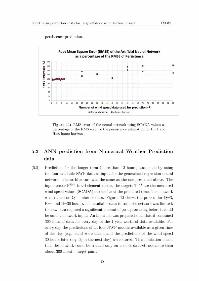
(5.4) The sensitivity of the prediction accuracy to the number of inputs (Q)

was tested and it was found that the precision does not increase above

several thousand inputs, therefore the final testing was carried out with

10000 training data. The prediction accuracy of the neural network was

tested for various numbers of past data used (R), and it was found that

using data of more than the last 12 hours decreases the performance of the

network (see figure 11). To evaluate the performance of the neural network,

the RMS error of the simulation was compared to the RMS error of the

persistance estimator. It was found that between about 4 and 8 hours

horizon the result of the neural network prediction using 2 to 8 previous

values shows a slight (no more than 5%) improvement compared to the

17


persistence prediction.

Figure 11: RMS error of the neural network using SCADA values aspercentage of the RMS error of the persistence estimation for H=4 andH=8 hours horizons.

5.3 ANN prediction from Numerical Weather Prediction

data

(5.5) Prediction for the longer term (more than 12 hours) was made by using

the four available NWP data as input for the generalised regression neural

network. The architecture was the same as the one presented above. The

input vector PR×1 is a 4 element vector, the targets T1×1 are the measured

wind speed values (SCADA) at the site at the predicted time. The network

was trained on Q number of data. Figure 12 shows the process for Q=3,

R=4 and H=30 hours). The available data to train the network was limited:

the raw data required a significant amount of post-processing before it could

be used as network input. An input file was prepared such that it contained

365 lines of data for every day of the 1 year worth of data available. For

every day the predictions of all four NWP models available at a given time

of the day (e.g. 9am) were taken, and the predictions of the wind speed

30 hours later (e.g. 3pm the next day) were stored. This limitation meant

that the network could be trained only on a short dataset, not more than

about 300 input - target pairs.

18


Figure 12: GRRN for NWP values. Example: Q=3, R=4, H=30.

(5.6) Due to the long horizon taken in this simulation, the comparison to per-

sistence is no longer a suitable method of evaluation (since its RMS error

is comparable to the standard deviation of the wind speed), therefore the

results are compared to the prediction made by taking the average of the

four NWP models. For large datasets of predictions it was found that the

RMS error of the average of the four NWP models was 1.5767 m/s. In

comparison, the neural network, after training on a few hundred data, pro-

duced predictions with RMS error of 1.3938 m/s. This is a significant 12%

improvement to the NWP average. (The standard deviation of the wind

speed was 2.271 m/s.)

(5.7) It is important to note that the accuracy of the predictions shows an increase

with higher amounts of training data, however, the increase is getting less

and less significant above about 150 training inputs. Training with more

diverse data (i.e predictions of different hours of the day, and predictions

from multiple years) and with a significantly higher number of data would

likely increase the performance of the neural network.

5.4 Remarks and possible future work

(5.8) The short term prediction with neural networks with a horizon of less than

12 hours using SCADA data provided a slight improvement over the simple

naive estimator. Other methods (e.g. ARMA) provided better results,

therefore application of neural networks for short term prediction by using

SCADA data alone does not seem practical.

19


(5.9) Longer term predictions (12-36 hours) were made using NWP data, and

an RMS error reduction of 12% was achieved on a horizon of 30 hours

compared to the average of the NWP data. The network was trained on a

small amount of data, each of them from the same hour of the day. More

diverse data and a higher number of input-target pairs would likely improve

the performance of the GRNN.

(5.10) From the achieved results it seems advisable to try and combine the inputs

from SCADA data and the NWP predictions on the short term and optimise

the performance by considering the usability of the methods on different

horizons. Combining the ANN’s with an ARMA model would likely give

optimal results for both long and short term predictions.

6 Kernel dressing

(6.1) Using the NWP point forecasts of the wind speed provided, we can produce

probabilistic forecasts that take account of the uncertainty around them.

We show how to build such forecasts and suggest ideas as to how they

could be improved.

(6.2) Suppose we wanted to predict the wind speed in 24 hours time. Whilst

any forecast has some uncertainty, we would expect to do reasonably well

running a model that uses some insight into the likely evolution of the

weather conditions from now until tomorrow. Now suppose we wanted to

predict the wind speed exactly a year from now. Running a model that

evolves today’s conditions for a whole year would give us a poor estimate

of the actual outcome, and any resemblance is simply from coincidence. In

reality, the best we can do without specific forecast information is to look at

some estimate of the long term distribution of wind speeds at that particular

point in time, so we might estimate the distribution from observations of

wind speed at this time of the day for the last 10 years. Alternatively, we

could look at the distribution of wind speeds just in the particular month

the day we are predicting the wind for falls. We may even look at wind

speed for the specific date of the year we are trying to predict over say the

last 100 years (although clearly this isn’t possible for wind farms). We call

these distributions ‘climatology’. Since we can always (when available) use

the climatology as a simple probabilistic forecast, it provides a lower bound

20


on how skillful we expect any model predictions for a specific day to be. A

model prediction that tends to give a worse forecast than climatology could

give us is of very little practical use. For this reason, we will always score

models relative to climatology.

(6.3) As we have discussed, the climatological distribution can take many forms.

Here, we discuss a few possible aproaches and settle on one which we use in

the rest of this section.

Figure 13: Climatological distribution over the entire year.

(6.4) Figure 13 shows a fit of the PDF of a normal distribution to the climatolog-

ical data from an entire year. This describes the distribution of windspeeds

over the entire year of data we are considering. Were we just making pre-

dictions of the wind speed in a particular month, we may want to use an

estimate based purely on the climatology for that month as shown in fig-

ure 14 for January or figure 15 for July. Ideally we would use the climatology

that is most specific to the forecasts we are considering however this is al-

ways balanced with availability of relevant data. In this report we use the

normal distribution obtained from an entire year’s data.

(6.5) An additional consideration is the choice distribution to be used in modelling

the climatology. We have used a Gaussian distribution as a first step due

21


Figure 14: Climatological distribution just using data from January.

Figure 15: Climatological distribution just using data from July.

to time constraints, however due to the complex nature of windspeed as a

variable it is likely that some other distribution would perform better.

(6.6) In order to choose between the various models that we will introduce in

this section, we need a way of comparing the effectiveness. The particular

22


method we use is the Ignorance Score. First introduced by IJ Good in

1952 [4], it is given by IGN = − log2 p where p is the amount of probability

placed on the eventual outcome. This particular skill score has desireable

properties for this kind of forecasting. For reasons discussed above, all

ignorance scores in this report are given relative to climatology, that is

IGNrel = IGN(mod)− IGN(clim).

(6.7) It is often beneficial to ‘blend’ a model with the Climatological distribution.

The reason this can be useful is that the climatology generally takes into

account all possible values the verification can take, whereas a model might

have a bias or be too narrow in its coverage. To do this, we simply take a

weighted average of the model and the climatology in the form:

P (y) = αPmod(y) + (1− α)Pclim(y) (6.1)

where Pmod(y) is the probabilistic forecast from the model and Pclim(y) is

an estimate of the distribution of the climatology. 0 < α < 1 is a parameter

that can be found by minimising the mean ignorance over a training set

(forecasts and verifications from the past).

(6.8) We introduce a number of simple probabilistic models for wind speed and

compare their skill using relative ignorance. All of these results correspond

to the most recent forecast available at 9am for 3pm the following day.

6.1 Running mean and variance normal distribution model

(6.9) Our first model is very simple. A probabilistic forecast is made using a

normal distribution with mean taken to be the average wind speed at 3pm

over the previous 5 days and the variance taken to be the variance of the

wind speed over the previous 30 days, i.e.

Model 1 - P (y) = N(mean(xt−1, ..., xt−5), var(xt−1, ..., xt−30)).

(6.10) We consider two cases, the model without blending (α = 1) and the model

blended with climatology (with optimal α with respect to the ignorance).

Since this model is very simplistic, we have no reason to expect it to perform

well, it is however useful for illustrative purposes in that using this model

on its own actually gives a positive relative ignorance, i.e. it does worse

than climatology. This is useful to note because realising this simple fact

23


enables us to disregard the model for any useful purposes. However, when

we blend the model with climatology, we find a slightly negative relative

ignorance albeit very close to 0. We see here, the benefits of blending with

climatology.

α Relative Ignorance1 0.38

0.3 -0.02

Table 2: Relative ignorance scores for running mean and variance model.

6.2 Individual Kernel Dressed Model forecasts

(6.11) For this model, we use the NWP data point forecasts provided. We use a

method called Kernel dressing which turns a set of points into a probability

distribution by replacing each one with some probability distribution called

a Kernel. The estimated PDF is then found by averaging the density of the

kernels at each point. In this case, where we have a single point forecast this

simply reduces to replacing the single point with a probability distribution.

Commonly, and this is what we do here, a Gaussian Kernel is used. For this

model, we assume that we have a learning set of forecasts and corresponding

verifications from which we can ‘tune’ our probabilistic forecast (although

due to lack of data to work with, this has been done in sample). The

mean of the distribution is taken to be the point forecast itself with a bias

correction found from the learning set (µi = fi − yi over the learning set)

and the standard deviation is taken as the standard deviation of the error

also found from the learning set (σi = std(fi − yi) also over the learning

set). Each probabilistic forecast is blended with climatology with the value

of α optimised with respect to the ignorance score. Formally, each model is

given by:

P (y) = N(fi − µi, σ2i ) (6.2)

where fi denotes the point forecast for NWP model i, µi is an offset param-

eter designed to correct the mean of the distribution and σi is the standard

deviation which is of course also a parameter.

(6.12) Here we find that the model using NWP1 forecasts performs the best fol-

lowed by the model using NWP2 forecasts. All of the forecasts give a

24


negative relative ignorance indicating that we improve on climatology in all

cases.

Forecast NWP1 NWP2 NWP3 NWP4Relative ignorance -0.93 -0.88 -0.67 -0.79

Table 3: Relative ignorance scores from using kernel dressing with each of thedifferent NWP data sources.

6.3 Possible future work

(6.13) In this section we have introduced a number of very simple models to create

probabilistic forecasts from point forecasts. Due to time constraints we

only considered normal distributions which may be unrealistic. Given more

time it would be beneficial to consider distributions that describe the data

better. Another step that would be highly beneficial in improving such

forecasts would be to use ensemble forecasts. Advanced methods exist that

convert ensembles to probability distributions with little assumption about

the properties of such distributions (See for example [2]). We would expect

such methods to perform very well for data of this kind.

7 Conclusions

(7.1) The optimal linear combination of the NWP forecasts was used as a bench-

mark for more advanced methods and resulted in RMS errors of 1.28-

1.68ms−1 for prediction windows of 4-48 hours. The 30 hour RMS error of

1.46ms−1 found for this method is slightly poorer than the corresponding

30 hour RMS error of 1.39ms−1 found using artifical neural networks. It

is possible that the artifical neural network does not add much predictive

value over a simple linear combination of forecasts although it is likely that

the artifical neural networks would perform better given a larger training

data set. Due to its complexity the 4D-Var method was not fully imple-

mented during the timeframe so we do not have results to compare with the

other forecasting methods. For shorter prediction windows (≈0-6 hours) the

ARMA model based only on the SCADA data appeared to give the smallest

RMS error although the comparison is with respect to smoothed data so it

is unclear how exactly this compares with the other methods. The output

of the kernel dressing method is a distribution rather than a point estimate.

25


Consequently its performance was measured in terms of relative ignorance

scores which are not directly comparable to the RMS errors used for the

other methods. It is unclear exactly how this compares with, for example,

the optimal linear combination.

(7.2) While the methods considered vary significantly in their complexity each

demonstrated some predictive value. However we have been unable to con-

clusively show that any of the methods provides a significant improvement

over the simplest method which involves taking the (optimal) linear combi-

nation of the available NWP forecasts at the time of interest.

Bibliography

[1] F. Bouttier and P. Courtier, Data assimilation concepts and methods,

Meteorological Training Course Lecture Series, (1999).

[2] J. Brocker and L. A. SMITH, From ensemble forecasts to predicitve distri-

butions, Tellus Series A, 60 (2008), pp. 663–678.

[3] R. Daley, Atmospheric Data Analysis, Cambridge Atmospheric and Space

Science Series, Cambridge University Press, Cambridge, UK, 1st ed., 1999.

[4] I. Good, Rational decisions, Journal of the Royal Statistical Society, 14 (1952),

pp. 107–114.

[5] E. Holm, Lecture notes on assimilation algorithms, Meteorological Training

Course Lecture Series, (2003).

[6] A. Lorenc, Analysis methods for numerical weather prediction, Quarterly Jour-

nal of the Royal Meteorological Society, 112 (1986), pp. 1177–1194.

[7] N. Nichols, Treating model error in 3-D and 4-D data assimilation, in Data

Assimilation for the Earth System, R. Swinbank, V. Shutyaev, and W. Lahoz,

eds., vol. 26 of NATO science series, Springer Netherlands, 2003, pp. 127–135.

26

Documents

Short term power forecasts for large offshore wind turbine