Embed Size (px)
Citation preview

University of Massachusetts Amherst University of Massachusetts Amherst
ScholarWorks@UMass Amherst ScholarWorks@UMass Amherst
Masters Theses 1911 - February 2014
2012
Probabilistic Analysis of Offshore Wind Turbine Soil-Structure Probabilistic Analysis of Offshore Wind Turbine Soil-Structure
Interaction Interaction
Wystan Carswell University of Massachusetts Amherst
Follow this and additional works at: https://scholarworks.umass.edu/theses
Part of the Geotechnical Engineering Commons, and the Structural Engineering Commons
Carswell, Wystan, "Probabilistic Analysis of Offshore Wind Turbine Soil-Structure Interaction" (2012). Masters Theses 1911 - February 2014. 848. Retrieved from https://scholarworks.umass.edu/theses/848
This thesis is brought to you for free and open access by ScholarWorks@UMass Amherst. It has been accepted for inclusion in Masters Theses 1911 - February 2014 by an authorized administrator of ScholarWorks@UMass Amherst. For more information, please contact [email protected].

PROBABILISTIC ANALYSIS OF OFFSHORE WIND TURBINE
SOIL-STRUCTURE INTERACTION
A Thesis Presented
by
WYSTAN CARSWELL
Submitted to the Graduate School of the
University of Massachusetts Amherst in partial fulfillment
of the requirements for the
MASTER OF SCIENCE IN CIVIL ENGINEERING
May 2012
Civil and Environmental Engineering

PROBABILISTIC ANALYSIS OF OFFSHORE WIND TURBINE
SOIL-STRUCTURE INTERACTION
A Thesis Presented
by
WYSTAN CARSWELL
Approved as to style and content by:
______________________________________
Sanjay R. Arwade, Chair
______________________________________
Don J. DeGroot, Member
______________________________________
Matthew A. Lackner, Member
_________________________________________
Richard N. Palmer, Department Head
Civil and Environmental Engineering Department

iii
ACKNOWLEDGMENTS
First and foremost, I would like to thank my family for their endless support. Knowing that they
are proud of my accomplishments is one of my biggest inspirations.
I would also like to thank my advisor, Sanjay R. Arwade, for his patience in helping me evolve
into the researcher I am today. Additionally, the perspective and commentary provided by my
thesis committee members, Matthew A. Lackner and Don J. DeGroot, were invaluable.
I am very appreciative of the education I received as an undergraduate at Lafayette College. The
support of my fellow alumni and former professors is a continual motivation for me to work hard
and aim high.
Lastly, it should be noted that this project was made possible by generous financial support from
the Brack Class of 1960 Graduate Fellowship.

iv
ABSTRACT
PROBABILISTIC ANALYIS OF OFFSHORE WIND TURBINE
SOIL-STRUCTURE INTERACTION
MAY 2012
WYSTAN CARSWELL, B.S., LAFAYETTE COLLEGE
M.S.C.E., UNIVERSITY OF MASSACHUSETTS AMHERST
Directed by: Sanjay R. Arwade
A literature review of current design and analysis methods for offshore wind turbine (OWT)
foundations is presented, focusing primarily on the monopile foundation. Laterally loaded
monopile foundations are typically designed using the American Petroleum Institute (API) p-y
method for offshore oil platforms, which presents several issues when extended to OWTs, mostly
with respect to the large pile diameters required and the effect of cyclic loading from wind and
waves. Although remedies have been proposed, none have been incorporated into current design
standards. Foundations must be uniquely designed for each wind farm due to extreme dependence
on site characteristics. The uncertainty in soil conditions as well as wind and wave loading is
currently treated with a deterministic design procedure, though standards leave the door open for
engineers to use a probability-based approach. This thesis uses probabilistic methods to examine
the reliability of OWT pile foundations. A static two-dimensional analysis in MATLAB includes
the nonlinearity of p-y soil spring stiffness, variation in soil properties, sensitivity to pile design
parameters and loading conditions. Results are concluded with a natural frequency analysis.

v
TABLE OF CONTENTS
Page
ACKNOWLEDGMENTS .............................................................................................................. iii
ABSTRACT .................................................................................................................................... iv
LIST OF TABLES ......................................................................................................................... vii
LIST OF FIGURES ........................................................................................................................ ix
LIST OF VARIABLES................................................................................................................. xiii
CHAPTER
1. INTRODUCTION AND LITERATURE REVIEW .................................................................... 1
1.1 P-y Method....................................................................................................................... 3
API Method for Cohesionless Soils ......................................................................... 4 1.1.1
P-y Curves for Cohesive Soils ............................................................................... 10 1.1.2
1.2 Current Design Practices ................................................................................................ 16
Foundation Types ................................................................................................... 17 1.2.1
Typical Dimensions ............................................................................................... 20 1.2.2
Design Standards ................................................................................................... 21 1.2.3
Limit States ............................................................................................................ 22 1.2.4
1.3 Uncertainty in Offshore Wind Turbine Design .............................................................. 25
1.4 P-y Curves for Large Diameter Piles ............................................................................. 26
1.5 Cyclic Loading in Offshore Wind Turbine Design ........................................................ 26
1.6 Conclusions .................................................................................................................... 28
2. STATIC TWO-DIMENSIONAL ANALYSIS .......................................................................... 30
2.1 Static Linear Analysis .................................................................................................... 32
2.2 Static Nonlinear Analysis .............................................................................................. 36
2.3 Conclusions .................................................................................................................... 38
3. PILE FOUNDATION RELIABILITY ...................................................................................... 40
3.1 Soil Variability ............................................................................................................... 41

vi
3.1.2. Variation in Friction Angle .................................................................................... 42
3.1.3. Variation in Relative Density ................................................................................. 43
3.1.4. Effect of Friction Angle on Pile Head Reaction .................................................... 45
3.2 Static Reliability Analysis .............................................................................................. 46
3.2.1 Correlated Friction Angle Variation ...................................................................... 47
3.2.2 Effect of Friction Angle Variance .......................................................................... 50
3.2.3 Effect of Friction Angle Distribution Shape .......................................................... 53
3.2.4 Effect of Pile Parameters........................................................................................ 57
3.2.5 Load Variation ....................................................................................................... 60
3.3 Conclusions .................................................................................................................... 64
4. LARGE DIAMETER EFFECTS ............................................................................................... 67
4.1 Conclusions .................................................................................................................... 68
5. NATURAL FREQUENCY ANALYSIS ................................................................................... 70
5.1 Deterministic Eigenvalue Problem ................................................................................ 72
5.1.1 NREL 5MW Reference Turbine Validation .......................................................... 72
5.1.2 Deterministic Parametric Studies ........................................................................... 76
5.2 Random Eigenvalue Problem......................................................................................... 84
5.3 Conclusions .................................................................................................................... 87
CONCLUSIONS AND RECOMMENDATIONS ........................................................................ 89
BIBLIOGRAPHY .......................................................................................................................... 94

vii
LIST OF TABLES
Table Page
1.1 Properties of Simplified Reference Pile ..................................................................................... 4
1.2 Reference Properties for Sand ................................................................................................... 6
1.3. Reference Properties for Soft Clay ......................................................................................... 11
1.4. Reference Properties for Stiff Clay ......................................................................................... 12
1.5 Representative Values of k for Stiff Clays (LPILE Plus 5.0, 2005) ........................................ 14
1.6 NREL 5MW Offshore Wind Turbine Properties (Jonkman, Butterfield, Musial, & Scott,
2009) .............................................................................................................................................. 21
2.1 Properties of Essen Sand (Lesny, Paikowsky, & Gurbuz, 2007) ............................................. 30
2.2 Properties of Pile Foundation (Lesny, Paikowsky, & Gurbuz, 2007) ...................................... 31
2.3. Applied Loads (Lesny, Paikowsky & Gurbuz, 2007) ............................................................. 32
2.4 Analysis Results from Linear Four-Spring Model for Pile Head Displacement...................... 33
2.5 Results from Linear vs. Nonlinear Comparison ....................................................................... 34
2.6 Pile Head Deflections from Nonlinear Analysis ...................................................................... 38
3.1 COV Ranges for Friction Angle (Phoon, 2008) ...................................................................... 42
3.2 Density Classification of Soil (Liu & Evett, 2004) .................................................................. 43
3.3 Comparison of Results from Correlation Limiting Cases ........................................................ 49
3.4 Beta Distribution Parameters to Examine Effect of Variance ................................................. 51
3.5 Mean and Standard Deviation of Friction Angle with Respect to Beta Parameters ................ 54
3.6 Beta Parameters Yielding Approximately 5% COV ................................................................ 56
3.7 Maximum and Minimum Reliability Indices Considering Pile Diameter and Wall
Thickness ....................................................................................................................................... 59
3.8 Loading Influence on Pile Head Response .............................................................................. 61
3.9 Reliability Index Results Considering Combinations of Load and Soil Randomness ............. 64

viii
5.1 Tower and Transition Piece Properties .................................................................................... 72
5.2 Dynamic Property Output for the NREL Reference Turbine .................................................. 76
5.3 Support Structure Wall Thicknesses, Considering Soil-Level Fixity ...................................... 79
5.4 Support Structure and Foundation Wall Thicknesses .............................................................. 82
5.5 Comparison of Unadjusted Dynamic Property Output for the NREL 5MW Reference
Turbine, Including Substructure and Monopile Foundation .......................................................... 83
5.6 Frequency Distribution Comparison of Soil Variation Cases .................................................. 86
5.7 Summary of Wall Thickness Increases .................................................................................... 87

ix
LIST OF FIGURES
Figure Page
1.1 Laterally-Loaded Pile ................................................................................................................. 3
1.2 Initial Modulus of Subgrade k as a Function of Friction Angle (DNV, 2009) .......................... 5
1.3 Coefficients as Function of Friction Angle (DNV, 2009).......................................................... 6
1.4 Force-Displacement Curves ....................................................................................................... 7
1.5 P-y Behavior with Respect to Internal Friction Angle ............................................................... 8
1.6 P-y Behavior with Respect to Unit Weight ................................................................................ 8
1.7 P-y Behavior with Respect to Pile Diameter ............................................................................. 8
1.8 P-y Behavior with Respect to Water Table Location................................................................. 9
1.9 Force-Displacement Curves for Soft Clay ............................................................................... 11
1.10 Force-Displacement Curves for Stiff Clay ............................................................................. 12
1.11 Comparison of Soft and Stiff Clay Force-Displacement Curves ........................................... 12
1.12 Comparison of Stiff Clay and Sand ....................................................................................... 13
1.13 Empirical Factors for Ultimate Resistance (Kramer, 1988) ................................................... 14
1.14 P-y Curves for Stiff Clay Below Ground Water Table .......................................................... 15
1.15 Saturated and Unsaturated Comparison of Stiff Clay p-y Behavior ...................................... 16
1.16 Basic Offshore Wind Turbine Diagram ................................................................................. 17
1.17 Types of Support Structures and their Applicable Water Depths (NREL, 2009) .................. 18
1.18 Monopile, Gravity Base, and Suction Bucket Foundations (Musial & Ram, September
2010) .............................................................................................................................................. 19
1.19 Offshore Wind Turbine Subjected to Lateral Loading .......................................................... 23
1.20 Depiction of Natural and Excitation Frequencies (de Vries & Krolis, 2004) ....................... 24
1.21 Depiction of One-Way and Two-Way Cyclic Loading ......................................................... 27
2.1 Force-displacement Curves for Four-Spring Essen Sand Model ............................................. 31

x
2.2 Four-Spring Pile Model ........................................................................................................... 33
2.3 Enlarged View of for Four-Spring Essen Sand Model with Linear Behavior ......................... 33
2.4 Number of Springs vs. Linear-Nonlinear Strength Difference ................................................ 35
2.5 Normalized Error vs. Number of Springs ................................................................................ 35
2.6 Single-Spring Model for Nonlinear Analysis .......................................................................... 36
2.7 Example 10-Step Nonlinear Analysis ...................................................................................... 37
2.8 Convergence of Nonlinear Analysis for Single-Spring Pile Model ......................................... 38
2.9 Convergence of Nonlinear Analysis for 20-Spring Pile Model ............................................... 38
3.1 Relative Density vs. Friction Angle ......................................................................................... 44
3.2 Normalized Pile Head Rotation as a Function of Friction Angle ............................................ 45
3.3 Normalized Pile Head Displacement as a Function of Friction Angle .................................... 45
3.4 Beta Probability Density Function, 5% COV .......................................................................... 48
3.5 Standard Deviation of Reliability Index vs. Number of Samples Considering Friction
Angle Variation .............................................................................................................................. 49
3.6 Histogram of Independent Variation Pile Head Rotation ........................................................ 50
3.7 Histogram of Perfect Correlation Pile Head Rotation.............................................................. 50
3.8 Beta Probability Density Functions Representing COVs 2-8.25% .......................................... 51
3.9 Reliability Index vs. COV of Friction Angle ........................................................................... 52
3.10 Mean Pile Head Rotation vs. COV of Friction Angle Distribution ....................................... 53
3.11 Reliability Surface Considering Beta Parameters, Independent Variation Case ................... 54
3.12 Reliability Surface Considering Beta Parameters, Perfect Correlation Case ......................... 54
3.13 Contour Plot of Reliability Indices with Respect to Beta Parameters , Independent
Variation Case ................................................................................................................................ 55
3.14 Contour Plot of Reliability Indices with Respect to Beta Parameters, Perfect Correlation
Case ................................................................................................................................................ 55
3.15 Contours of Friction Angle COV with Respect to Beta Parameters ...................................... 56
3.16 Beta Probability Density Functions with Approximately 5% COV per Table 3.5 ................ 56

xi
3.17 Reliability Index vs. Mean Friction Angle ............................................................................. 57
3.18 Reliability Surface Considering Pile Diameter and Wall Thickness, Independent
Variation Case ................................................................................................................................ 58
3.19 Reliability Surface Considering Pile Diameter and Wall Thickness, Perfect Correlation
Case ................................................................................................................................................ 58
3.20 Contours of Reliability and Moment of Inertia, Independent Variation Case ....................... 59
3.21 Contours of Reliability and Moment of Inertia, Perfect Correlation Case............................. 59
3.22 Reliability Index vs. Embedment Depth ................................................................................ 60
3.23 Standard Deviation of Reliability Index vs. Number of Samples Considering Load
Variation ........................................................................................................................................ 62
3.24 Comparison of Load and Friction Angle Convergence Figures ............................................ 63
3.25 Comparison of Convergence Studies Considering Combinations of Load and Soil
Randomness ................................................................................................................................... 63
4.1 Reliability Index vs. Reference Diameter ................................................................................ 68
4.2 Reliability Index vs. Adjusted Initial Modulus of Subgrade (k*) ............................................ 68
5.1 Structural Design Regime for Offshore Wind Turbines (Petersen, et al., 2010) ..................... 70
5.2 Example Finite Element with Illustrated DOFs ....................................................................... 74
5.3 Convergence of Third Mode Frequency for NREL 5MW Reference Turbine ........................ 75
5.4 Dimensions of NREL 5MW Reference Turbine in North Sea Conditions .............................. 76
5.5 Convergence of Third Mode Natural Frequency for NREL 5MW Reference Turbine,
Including Transition Piece ............................................................................................................. 77
5.6 Effect of Wall Thickness on Natural Frequency, Considering Tower and Substructure ......... 78
5.7 Natural Frequency Contour Plot, in Reference to Support Structure Wall Thickness ............. 79
5.8 Comparison of Support Structure Volume and Natural Frequency Contours ......................... 79
5.9 Convergence of First Natural Frequency with Regard to Infinitely Stiff Soil Springs ............ 80
5.10 Convergence of First Natural Frequency with Respect to Soil Springs ................................. 80
5.11 Natural Frequency Contour Plot with Respect to Wall Thickness, Including Monopile
Foundation ..................................................................................................................................... 81
xii
5.12 Comparison of Volume and Natural Frequency Contours of Support Structure and
Monopile Foundation ..................................................................................................................... 81
5.13 Effect of Embedment Depth on Third Natural Frequency ..................................................... 82
5.14 First Natural Frequency vs. Friction Angle ........................................................................... 83
5.15 Convergence of Standard Deviation of First Natural Frequency ........................................... 85
5.16 First Natural Frequency Distribution Comparison of Soil Variation Cases, 1000 Samples .. 85
5.17 Offshore Wind Turbine Frequency Compared to Excitation Frequencies (Petersen, et al.,
2010) ............................................................................................................................................ 856

xiii
LIST OF VARIABLES
A Beta distribution parameter
a Cross-sectional area
As, Ac Variable used for p-y curves, (static, cyclic)
B Beta distribution parameter
b Pile diameter
C𝜑’𝜑’ Covariance
C1, C2, C3 Variables in the API method selected from figures
d Pile embedment depth
DR Relative density
Ds Boundary condition matrix
E Modulus of elasticity
E(x) Oedemetric modulus (mean stress range)
e, emax, emin Void ratio (maximum, minimum)
F𝜑’ Cumulative distribution function
fn Natural frequency (Hz), where n is the mode number
g1, g2 Safety margins (horizontal pile head displacement, pile head rotation)
H Horizontally-applied load
I Moment of inertia
J Polar moment of inertia
k Initial modulus of subgrade reaction
K Global stiffness matrix
Lo Adjusted Pile depth
LR Linear soil-pile resistance
m Element mass matrix
M Applied moment

xiv
M Global mass matrix
N Normal (Gaussian) distribution
NLR Nonlinear soil-pile resistance
p Pile resistance (force/length)
pf Probability of failure
pu, pus, pud Ultimate pile resistance
su Undrained shear strength
u Horizontal pile head displacement
V Vertically-applied load
V Displacement column vector
x Vertical direction
xk Vertical distance between soil springs
y Horizontal direction
y50 Horizontal deflection and 50% of ultimate soil resistance
𝛼 Pile head rotation
𝛽 Reliability index
𝛾 Total unit weight
𝛿 Correlation length
𝜖50 50% of maximum principle stress difference
Large diameter effect factor
𝜇 Mean value
𝜌 Mass density
𝜎 Standard deviation
𝜑’ Friction Angle
𝜔 Frequency (rad)

1
CHAPTER 1
INTRODUCTION AND LITERATURE REVIEW
Offshore wind turbine (OWT) design is a burgeoning area of engineering with roots in the
development and research of offshore drilling platforms by the American Petroleum Institute
(API) performed in the 1970s. Given recent demands for renewable energy, more attention has
been paid to offshore options with the majority of research performed in Europe on OWTs in the
North Sea.
Monopiles are the most popular foundation type for OWTs due to the simplicity of load path and
definition for wind and wave loading. Laterally loaded monopile foundations are typically
designed using the p-y method for analysis of the soil-structure interaction, developed by API.
The p-y method is based on a distributed-spring model, which varies according to soil
classification, properties, and location in reference to the water table.
While towers are classified and manufactured typically by turbine rating, foundations must be
uniquely designed for each wind farm due to their strong dependence on site characteristics.
Unique foundation design is time-consuming with important financial implications. Uncertainty
in soil conditions as well as wind and wave loading is currently treated with a deterministic
design procedure, though the Det Norske Veritas (DNV) design standard leaves the door open for
engineers to use a probability-based approach, which could prevent unnecessary use of materials
due to overdesign.
Several problems are inherent in the application of the API p-y method for OWTs, as the method
was developed for monotonic loading of small-diameter piles. This leads to inaccurate modeling
of large diameter OWTs subjected to cyclic loading of wind and waves. Research has been

2
performed on these discrepancies, but as of yet no adjustments have been incorporated into the
design standards.
This thesis uses probabilistic methods to quantify the randomness inherent in wind and wave
loading, as well as variability in soil conditions. A two-dimensional monopile model was
developed in MATLAB to monitor soil-pile interaction, particularly with reference to pile head
rotation.
Under quasi-static loading conditions, the effect of variable soil properties was studied using first
order reliability method. Relative density was related to friction angle using the relationship
implied by API figures, considering friction angle to be the only varying soil property and all
others to be deterministic. Using Monte Carlo simulation to estimate the reliability index (which
is related to the probability of failure), the effects of friction angle variance and mean were
analyzed for medium-dense to dense sands. The limiting soil property correlation cases of
independent variation and perfect correlation are shown to demonstrate the range of potential
reliability indices.
After observing how reliability changes with soil properties, a sensitivity analysis was conducted
to identify how OWT monopile reliability is effected by pile diameter, wall thickness and
embedment depth. This analysis is followed by a brief discussion of large pile diameter effects.
The National Renewable Energy Laboratory (NREL) 5MW Reference Turbine was modeled in
MATLAB. By solving the characteristic eigenvalue problem to obtain natural frequency, the
effect of soil property variability was examined again.
In conclusion, this thesis describes a summary of findings and recommendations for future work.

3
1.1 P-y Method
The lateral soil-structure behavior of pile foundations is usually characterized using p-y curves.
Each curve is defined by a unit lateral load (p, in units of force per length) and lateral
displacement of the pile (y) in response to loading (e.g., Figure 1.1). The p-y method is based on
the Winkler Foundation Theory, which describes soil response as a series of springs. Also called
a Distributed Spring model, it was recommended by Bush & Manuel (2009) as well as Bir &
Jonkman (2008) as it “most closely represents the true monopile configuration” (Bir & Jonkman,
2008). Winkler Theory assumes semi-infinite pile length as well as constant stiffness of soil and
pile (i.e., uniform properties). For pile models such as the one in Figure 1.1, we will consider the
difference in depth between each sequential soil spring to be xk meters.
Figure 1.1 Laterally-Loaded Pile
The API method for sand, Matlock’s method for soft clay, and Reese et al.’s method for stiff clay
use similar soil and pile properties to represent p-y soil-structure interaction. For the following p-
y curve examples, we will consider a reference pile such as the one in Figure 1.1 with the
properties listed in Table 1.1 in order to compare the effects of certain soil properties, water table
location, and pile diameter variation.
Ground Surface P
xk
y
x

4
Table 1.1 Properties of Simplified Reference Pile
Symbol Property Value
b Pile Diameter 1 meter
d Pile Depth 10 meters
xk Distance between Soil Springs 2.5 meters
API Method for Cohesionless Soils 1.1.1
The majority of research done on offshore pile foundations has been done by the oil and gas
industry for offshore platforms in the 1970s and 1980s (LeBlanc, Houlsby, & Byrne, 2010). The
API method for determining p-y curves in sand was based on the ultimate resistance (pu in
dimensions of force per unit length) established originally by Reese et al. (1975) and then
checked by O’Neill and Murchison (LeBlanc, Houlsby, & Byrne, 2010). The API method,
described in API RP2A, is fundamentally influenced by the angle of internal friction φ’, total soil
unit weight γ, and pile diameter b, where
(
)
(1.1)
where A is either As or Ac:
(
) for static loading
Ac = 0.9 for cyclic loading
(1.2)
and the initial modulus of subgrade k is obtained from Figure 1.2 as a function of φ’ and water
table location.

5
Figure 1.2 Initial Modulus of Subgrade k as a Function of Friction Angle (DNV, 2009)
The ultimate soil resistance at a selected depth, pu, is given by
(1.3)
𝛾
(1.4)
𝛾 (1.5)
where pus is the ultimate soil resistance at shallower depths, pud is the ultimate soil resistance at
deeper depths, and C1 and C2 are coefficients determined as a function of φ’ from Figure 1.3.

6
Figure 1.3 Coefficients as Function of Friction Angle (DNV, 2009)
Using the four-spring reference model (Fig. 1.1, Table 1.1), the soil properties from Table 1.2,
and assuming the water table is located below the pile, the API method yields four curves – one
for each spring.
Table 1.2 Reference Properties for Sand
Symbol Property Value/Description
φ’ Angle of Internal Friction 35°
γ Total Soil Unit Weight 17 kN/m3
k Initial Modulus of Subgrade Reaction 38 MPa
Since the p values are in units of force per unit length, they are multiplied by the tributary length
along the pile, xk, in order to create a curve of lateral force (kN) versus displacement (m) such as
in Figure 1.4.

7
Figure 1.4 Force-Displacement Curves
Figure 1.4 illustrates clearly that the initial stiffness and soil strength increases with depth. It can
be seen by visual inspection of Equations 1.4 and 1.5 that increasing φ’, γ, or b will also cause the
strength of the soil to increase. Using the force-displacement curve representing the bottom pile
spring from Figure 1.4 as a baseline for comparison, we can see how the behavior of p-y curves is
affected by adjusting φ’, γ, or b to approximately ±15% of the control variables.
In the case of Figure 1.5, we note the difference in ultimate strength when 𝜑’ is equal to 30°, 35°,
and 40° - classified by friction angle alone, these sands could be respectively considered loose
sand, medium sand, and dense sand (Van Nostrand Reinhold, 2002). When 𝜑’ is increased from
35° to 40°, the basic shape of the force-displacement curve remains unchanged but the soil-pile
resistance increases by approximately 1x10⁴ kN. Decreasing 𝜑’ from 35° to 30° results in a
similar decrease in soil-pile resistance but also “softer” curve (decreased initial stiffness).

8
Figure 1.5. P-y Behavior with Respect to Internal
Friction Angle
Figure 1.6. P-y Behavior with Respect to Unit Weight
Altering the total unit weight, 𝛾, of the soil has much less of an effect than changing the friction
angle. Figure 1.6 shows that a 15% change in total unit weight results in a soil-pile resistance
difference of 0.25x10⁴ kN.
Figure 1.7. P-y Behavior with Respect to Pile Diameter
Soil-pile resistance differences resulting from a 15% change in pile diameter demonstrated in
Figure 1.7 are very minimal.
9
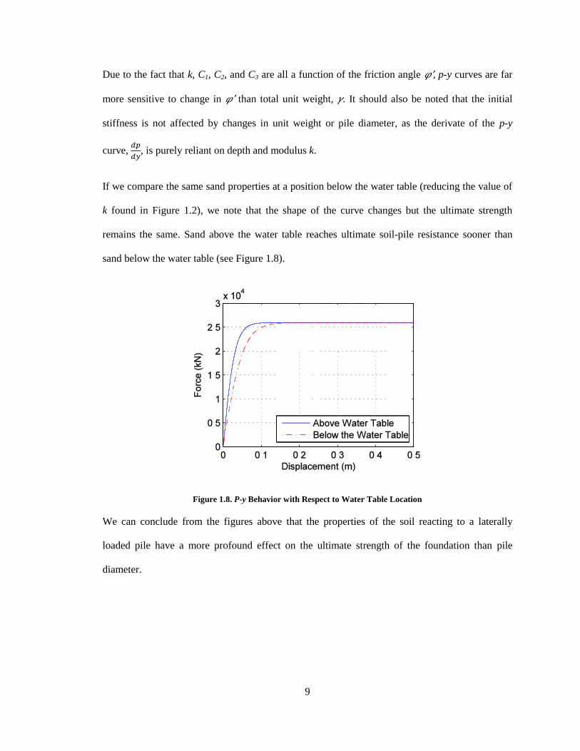
Due to the fact that k, C1, C2, and C3 are all a function of the friction angle 𝜑’, p-y curves are far
more sensitive to change in 𝜑’ than total unit weight, 𝛾. It should also be noted that the initial
stiffness is not affected by changes in unit weight or pile diameter, as the derivate of the p-y
curve,
, is purely reliant on depth and modulus k.
If we compare the same sand properties at a position below the water table (reducing the value of
k found in Figure 1.2), we note that the shape of the curve changes but the ultimate strength
remains the same. Sand above the water table reaches ultimate soil-pile resistance sooner than
sand below the water table (see Figure 1.8).
Figure 1.8. P-y Behavior with Respect to Water Table Location
We can conclude from the figures above that the properties of the soil reacting to a laterally
loaded pile have a more profound effect on the ultimate strength of the foundation than pile
diameter.
10
It should be noted that generally friction angle increases with unit weight, and the two quantities
are not independent of one another (Day, 2000). Thus, the cases shown above should be
considered only for qualitative purposes.
P-y Curves for Cohesive Soils 1.1.2
Cohesive soils, or clays, behave differently under lateral loading than cohesionless soils.
Cohesionless soils below the ground water table require a reduced initial modulus of subgrade;
for cohesive soils, an entirely different set of equations are required to illustrate p-y behavior.
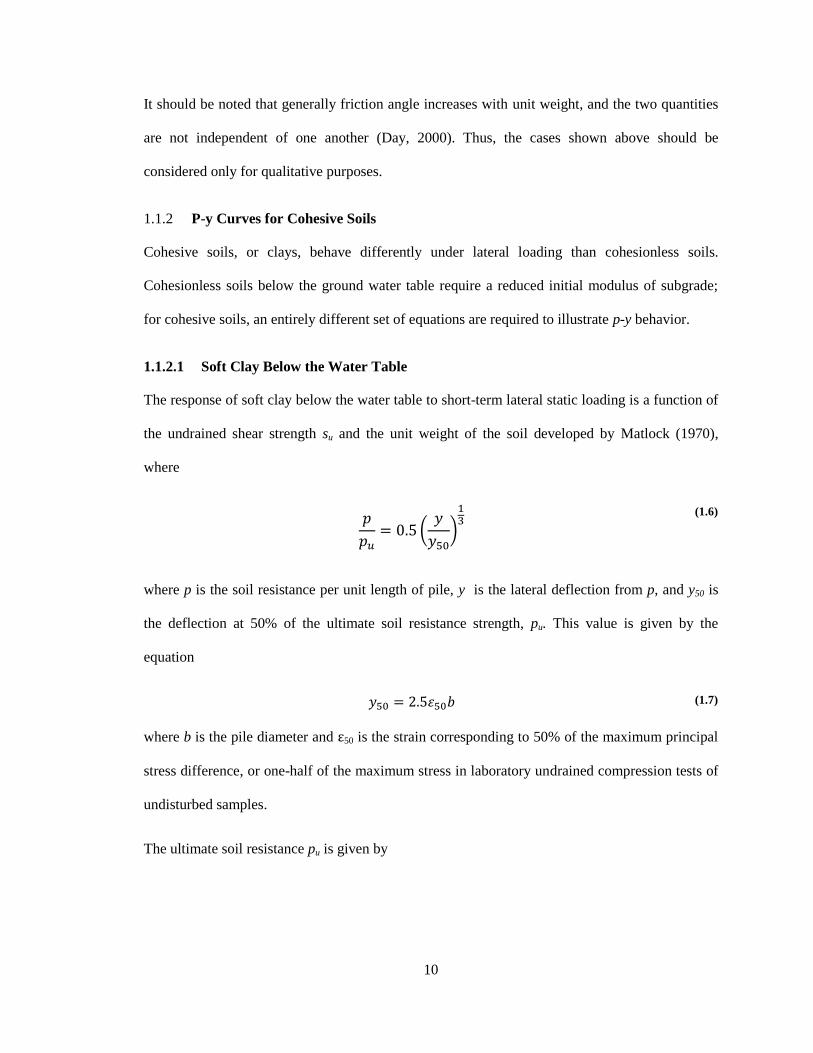
1.1.2.1 Soft Clay Below the Water Table
The response of soft clay below the water table to short-term lateral static loading is a function of
the undrained shear strength su and the unit weight of the soil developed by Matlock (1970),
where
(
)
(1.6)
where p is the soil resistance per unit length of pile, y is the lateral deflection from p, and y50 is
the deflection at 50% of the ultimate soil resistance strength, pu. This value is given by the
equation
휀 (1.7)
where b is the pile diameter and ε50 is the strain corresponding to 50% of the maximum principal
stress difference, or one-half of the maximum stress in laboratory undrained compression tests of
undisturbed samples.
The ultimate soil resistance pu is given by

11
(1.8)
* 𝛾
+
(1.9)
(1.10)
where 𝛾’ is the average effective unit weight from ground surface to the soil spring, x is the depth
to the soil spring, and su is the undrained shear strength at depth x. The variable J is typically 0.5.
Using the reference four-spring model, force-displacement curves from the properties listed in
Table 1.3 would appear as in Figure 1.9.
Table 1.3. Reference Properties for Soft Clay
Property Value
γ’ 6 kN/m3
su 20 kN/m3
J 0.5
Figure 1.9. Force-Displacement Curves for Soft Clay
1.1.2.2 Stiff Clay Above the Water Table
The Reese, Cox and Koop (1975) p-y curve development procedure for stiff clay above the water
table is based on lateral load tests similar to Matlock’s, differing from soft clay only in exponent:
¼ instead of ⅓ (see Equation 1.11).
(
)
(1.11)

12
However, the ultimate strength displacement limit is twice that of soft clay: p = pu for y > 16y50.
Table 1.4. Reference Properties for Stiff
Clay
Property Value
γ 19 kN/m3
su 100 kN/m3
J 0.5
Figure 1.10. Force-Displacement Curves for Stiff Clay
For the values in Table 1.4, the stiff clay force-displacement curves would appear as in Figure
1.10. If we compare both soft and stiff clays (as in Figure 1.11), we note that stiff clay can
provide significantly more soil-pile resistance than the soft clay.
Figure 1.11 Comparison of Soft and Stiff Clay Force-Displacement Curves

13
As seen in Figure 1.12, this sample of stiff clay cannot provide as much soil-pile resistance as
sand – in this case, the lowest spring is weaker by a factor of 5. However, for the reference values
chosen, the soil resistance difference from the top spring to the bottom spring is much smaller for
stiff clay than sand.
Figure 1.12 Comparison of Stiff Clay and Sand
1.1.2.3 Stiff Clay Below the Water Table
The method for developing p-y curves for stiff clay in the presence of free water is significantly
different than stiff clay above the water table. The curve is segmented into several different
sections which are characterized by
(1.12)
𝛾
(1.13)
(1.14)
Where su is the average undrained shear strength over the depth x, b is the pile diameter, and 𝛾’ is
the submerged, or effective soil unit weight. Depending on the normalized depth (i.e., depth to the

14
soil spring divided by the total pile length), a value of As is selected from Figure 1.13 (B
represents the coefficient required for the cyclic process, not described here).
Figure 1.13 Empirical Factors for Ultimate Resistance (Kramer, 1988)
The initial straight-line portion of the p-y curve is described by
(1.15)
where k is obtained from Table 1.5.
Table 1.5 Representative Values of k for Stiff Clays (LPILE Plus 5.0, 2005)
Average Unconsolidated Undrained Shear Strength
su (kPa) 50-100 100-200 300-400
k (static, MN/m3) 135 270 540
The next portion of the curve begins at the intersection of the straight line and the parabolic curve

15
(
)
(1.16)
where
휀 (1.17)
The third portion of the p-y curve begins when y is equal to Asy50 and extends to y equal to 6Asy50.
(
)
(
)
(1.18)
From y equals 6Asy50 to y equals 18Asy50,
√
(1.19)
After 18Asy50,
√ (1.20)
Given the same characteristics described in Table 1.4 for stiff clay above the water table, the p-y
curves for the simple four-spring model appear as in Figure 1.14.
Figure 1.14 P-y Curves for Stiff Clay Below Ground Water Table

16
Note that the range of displacement shown is only from 0 to 0.02 m.
Figure 1.15 Saturated and Unsaturated Comparison of Stiff Clay p-y Behavior
When stiff clay becomes saturated, the difference in p-y behavior is very obvious (see Figure
1.15). While the resistance of the pile for saturated stiff clay peaks earlier than unsaturated stiff
clay, pile resistance drops almost immediately afterwards. The ultimate soil-pile resistance for the
bottom spring in unsaturated stiff clay, in this instance, is greater by a factor of approximately 1.5
and is sustained after a displacement of 0.2 m.
1.2 Current Design Practices
Offshore wind turbines (OWTs) are comprised of a nacelle (hub that houses the mechanical
components, including rotor), rotor blades, tapering transition tower section, tower, and
foundation (see Fig. 1.16). The towers are usually made in 20-30 m long sections (limited by
transportation) of rolled and welded steel plate, while the rotor blades are made of fiberglass
(Malhotra, 2010).

17
Figure 1.16 Basic Offshore Wind Turbine Diagram
Increasing renewable energy production demands that OWTs in the United States need to be
5MW or greater for economic feasibility, requiring wind farms to move out to depths of 30-50 m
where wind speeds are higher and more uniform. As of 2008 however, 40% of OWTs were rated
at 1.5MW or higher with the typical range being 2.0 to 3.6MW (Bolinger & Wiser, 2008),
(Department of Energy, 2010).
While the tower designs are specified by maximum power output, foundations are entirely site
specific due to dependency on environmental and soil factors. These factors include scour, water
depth, marine growth, sea ice, wind, wave, and soil profile data.
Foundation Types 1.2.1
Offshore wind turbine foundations are chosen mostly by water depth, as hydrodynamic loading
generally dominates design. Depths are separated into the categories of deep, shallow, and
transitional (see Fig.1.17).
Hub/Nacelle Rotor blades
Monopile Foundation
Transition Piece

18
Figure 1.17. Types of Support Structures and their Applicable Water Depths (NREL, 2009)
The large mass and inertia of the gravity foundation (see Figure 1.18, center) have been found
attractive for the rough conditions of the North Sea, given that installation does not require
specialized vessels (Stancich, 2010). However they are limited to feasible installation depths of
less than 20 m and require extensive site preparation (Malhotra, 2010). Minimizing structural
dead weight for gravity foundations (while also providing sufficient dead weight) is challenging
(Thomsen, Forsberg, & Bittner, 2007).

19
Figure 1.18. Monopile, Gravity Base, and Suction Bucket Foundations (Musial & Ram, September 2010)
Suction caissons (or buckets, see Figure 1.18 right) are time-consuming and labor-intensive to
install as well as having limited installation depths (Malhotra, 2010). Suction caissons perform
optimally in soft clay situations where a seal can form around the caisson during suction in the
installation process; any soil material that is prone to fissures can inhibit the formation of a seal
and therefore is unsuitable (Houlsby & Byrne, 2005).
The monopile design (see Figure 1.18, left) is simple, providing a direct load path from the tower
to the soil and clearly defined loading from wind and waves. While installation can be noisy,
monopiles are otherwise considered to have the least environmental impact on marine ecologies
due to their unobtrusive geometry – also an advantage regarding damage risks in the event of ship
collision (Abdel-Rahman & Achmus, 2005). There is some disagreement in reference to the
Monopile Gravity Base Suction Bucket

20
depths at which a monopile is appropriate, but it is the overwhelmingly popular choice for OWTs
and will thus be the focus of this study. It is generally agreed that monopiles are feasible for
depths up to 30m, though some would say even up to 40 or 50 m (Lesny & Hinz, 2007; Malhotra,
2010).
The challenge of installation dictates the depths to which monopiles are feasible, as the jack-up
installation barges currently used have a maximum water depth of 25-30 m; however, new
techniques have allowed installation up to 45 m (Musial & Ram, September 2010). For anything
in excess of 45 m, innovation in floating platform foundations may be the answer (Musial &
Ram, September 2010).
Multi-pile substructures (such as tripods) are typically used for depths that exceed the practical
limits of monopiles. Tripod foundations are considered to be the “most promising” foundation for
depths greater than 30 m, but monopiles may be an alternative (Abdel-Rahman & Achmus,
2005).
Typical Dimensions 1.2.2
A typical monopile foundation has a 4-m diameter and penetration depth up to 18 m, with a
length/diameter ratio of approximately 5 (LeBlanc, Houlsby, & Byrne, 2010). However, in order
to support the loading incurred by a 5MW OWT, diameters can be as large as 8 m with wall
thicknesses up to 60 mm. Wall thickness to diameter ratios of a typical monopile are typically
1:50 to 1:80 (LeBlanc, Houlsby, & Byrne, 2010), (de Vries & Krolis, 2004).
Despite vast offshore wind resources, there are no offshore wind turbines in the United States to
date due primarily to cost, but also regulatory and permitting issues (Musial & Ram, September
2010). However, the National Renewable Energy Laboratory (NREL), a research laboratory of
the U.S. Department of Energy, has sponsored several studies on OWTs. In order to “support

21
concept studies aimed at assessing offshore wind technology”, the NREL 5MW baseline wind
turbine was created from a compilation of several manufactured models (Jonkman, Butterfield,
Musial, & Scott, 2009). This study will use the specifications of the NREL 5MW baseline OWT
with properties listed in Table 1.6.
Table 1.6 NREL 5MW Offshore Wind Turbine Properties (Jonkman, Butterfield, Musial, & Scott, 2009)
Property Value
Rotor, Hub Diameter 126 m, 3 m
Hub Height 90 m
Tower Base Diameter & Wall Thickness 6 m, 0.027 m
Tower Top Diameter & Wall Thickness 3.87 m, 0.019 m
Young’s and Shear Modulus of Steel 210 GPa, 80.8 GPa
Cut-In, Rated, Cut-Out Wind Speed 3 m/s, 11.4 m/s, 25 m/s
Cut-In, Rated Rotor Speed 6.9 rpm, 12.1 rpm
Rated Tip Speed 80 m/s
Overhang, Shaft Tilt, Precone 5 m, 5°, 2.5°
Rotor Mass 110,000 kg
Nacelle Mass 240,000 kg
Tower Mass 347,460 kg
It is assumed that the tower tapers linearly from the base properties to the top properties
(Jonkman, Butterfield, Musial, & Scott, 2009).
Design Standards 1.2.3
Design standards are currently region-based. Both Germany and Denmark have national design
standards for OWTs, but the majority of OWT foundation design relies on the American
Petroleum Institute Recommended Practice 2A (API RP 2A), International Design Standard for

22
Offshore Wind Turbines (IEC 61400-3), Det Norske Veritas (DNV), and Germanischer Lloyd
(GL) design documents. As of December 2010, the American Bureau of Shipping (ABS)
released a guide for building and classing of offshore wind turbine installations, which is based
primarily on API standards and IEC 61400-3.
Unlike the other design standards, API RP 2A was compiled in reference to fixed offshore
platforms as opposed to offshore wind turbines. As such, it includes a higher level of detail in
design due to life safety concerns and the delicacy of offshore drilling. However, the API p-y
method is used by all of the design standards for designing monopile foundations.
The design standards typically cite a return period of 50 years in reference to extreme wind and
wave loading, though ABS uses a 100-year return period. These return periods are intended to
designate the design lifetime of the structure, though the IEC 61400-3 uses a 50-year return
period but states a design lifetime of 20 years (IEC 61400-3, 2009).
While the primary design methods are deterministic with partial safety factors (ranging from 1.0
to 1.5, applied to both loads and materials) for most design standards, some standards also allow
for the use of probabilistic methods. The DNV (2009) standard allows for calibrating
deterministic design methods or for special designs with which there is limited experience, the
GL (2005) standard for the designer to use probabilistic methods of analysis with consultation,
and ABS (2010) for obtaining environmental condition values.
Limit States 1.2.4
This thesis will focus on the pile foundation of the OWT which is designed to support the
sustained weight of the hub, nacelle, tower and transition piece. In addition to withstanding these
deterministic gravity loads, the foundation must resist stochastic loading from wind and waves
(see Fig 1.19). While axial loading is taken into consideration, hydrodynamic lateral loading is

23
generally governing (de Vries & Krolis, 2004). The tower is designed for extreme load cases
initially, and then operational load cases are checked (Lesny & Hinz, 2007).
Figure 1.19 Offshore Wind Turbine Subjected to Lateral Loading
As considering the extreme state of both wind speed and wave height simultaneously is
considered too conservative, extreme wind gusts are taken into account with reduced wave
heights; a process very reminiscent of traditional load and resistance factor design where extreme
events are not considered to occur simultaneously (Quarton, 2005). The design cases considered
are when wind and waves are aligned (co-directional) and when acting from a single worst case
direction (uni-directional) (Quarton, 2005).
Design standards define limit state levels in different ways, though the most commonly
referenced are the Serviceability Limit State (SLS) and Ultimate Limit State (ULS), where SLS is
defined by the DNV as “deflections that may prevent intended operation of equipment” and ULS
refers to structural failure (DNV, 2009).
The main structural limit states considered depend on resistance to cyclic/dynamic loading and
mudline rotation. Cyclic loading from wind, waves, and mechanical vibrations are a major factor
Wind Loading
Wave Loading

24
in design considerations. Mechanical vibrations are classified into two main frequency intervals
referred to as 1P and 3P, for the excitation caused by the rotation of one rotor blade and the
combination of all three rotor blades, respectively (see Fig. 1.20 for the Vestas V90 3.0 MW wind
turbine situated in the North Sea).
Figure 1.20 Depiction of Natural and Excitation Frequencies (de Vries & Krolis, 2004)
After the natural period for the tower has been selected to avoid resonance, the diameter and wall
thickness of the tower are designed to withstand environmental factors (such as marine growth
and ice) as well as standard loading. After the general properties are selected to prevent buckling,
sufficient embedment depth of the monopile foundation is required. Embedment depths to
prevent foundation failure are defined by the equation
√
(1.21)
wheretypically varies between 4 and 5, J is the polar moment of inertia, b is the diameter of the
pile, and k is the initial modulus of subgrade and

25
(
)
(1.22)
where E(x) is the oedemetric modulus (mean stress range) which, for Essen Sand, is 50-80
MN/m2 (Lesny, Paikowsky, & Gurbuz, 2007).
After sufficient embedment depth is achieved, mudline rotation must be minimized in order to
keep the wind turbine within efficient operational levels. Wiemann, Lesny & Richwien (2004)
state that the pile head rotation cannot exceed 0.7° and still be considered a rigid foundation,
which is a standard design assumption. In addition to this, the GL standard used by de Vries &
Krolis (2004) restricted horizontal displacement at the mudline to 0.2 m.
1.3 Uncertainty in Offshore Wind Turbine Design
Uncertainty in OWT design is currently treated by using conservative deterministic methods.
Since the random loading of wind and waves dominate design, conservatism leads to larger (and
therefore more expensive) towers and foundations.
Towers are designed for particular return periods for both the wind and waves according to
metocean data, and the towers are assumed to have a lifetime equivalent to these return periods.
In addition to the uncertainty in wind and wave loading, soil is a large source of uncertainty since
it is not a homogeneous material. Site characterization often calls for at least one boring in the
installation area, with more specific site tests per requirement of the applicable design standard,
providing designers with the general soil profile of the wind farm site. Not only is the soil
variable, but the measurement methods utilized are also uncertain.

26
In an assessment on the Platform Cognac (a deep-water platform installed in 1978 according to
API standards), it was determined that the largest source of bias occurred in the foundation
stiffness, from estimations of clay strength and stiffness (Gur, Choi, Abadie, & Barrios, 2009).
1.4 P-y Curves for Large Diameter Piles
The API method for determining p-y curves was based on testing of slender piles of 0.6-m
diameter and confirmed for pile diameters up to 2 m (Wiemann, Lesny, & Richwien, 2004).
Despite its limitations, monopiles with diameters up to 4.5 m have been installed using this
method. Studies show that the API method greatly overestimates the stiffness at large depths for
large-diameter piles, resulting in insufficient embedment lengths for the piles and negates the
design assumption that the OWT tower is rigidly affixed in the soil (Lesny & Wiemann, 2005),
(Krolis, van der Tempel, & de Vries, 2007). This overestimation in soil strength can lead to pile
deflection underestimation of up to 120% (Lesny, Paikowsky, & Gurbuz, 2007).
For significant pile deformations, shear stresses are induced around the perimeter of the
foundation which the API p-y method does not take into account for large diameter piles (Lesny,
Paikowsky, & Gurbuz, 2007).
Lesny & Wiemann (2006) suggest a modification for large diameter open pipes, but it has not yet
been adopted by design standards.
1.5 Cyclic Loading in Offshore Wind Turbine Design
Cyclic loading of OWTs impacts both the tower and foundation. The structural integrity of the
tower can be compromised by way of fatigue or damage caused by resonance, with the most
challenging aspect of modeling being the randomness of wind and wave loading.

27
Unlike structural components, the modeling of cyclic effects on soil requires the incorporation of
randomness in both the loading and the material. Cyclic loading causes the soil surrounding the
monopile foundation to develop plastic strains. As the life of the OWT proceeds, the stiffness of
the foundation decreases. This decrease in stiffness increases deflection and rotation, hampering
the efficiency of the turbine operation and increasing the possibility of failure (Lesny & Hinz,
2007).
LeBlanc, Houlsby, & Byrne (2010) performed long-term cyclic studies on 80.0 mm piles in sand.
According to their results, stiffness increased with the number of cycles independent of relative
density for undrained piles; however, further work is necessary to examine how applicable these
results are for larger piles (LeBlanc, Houlsby, & Byrne, 2010).
Wind is modeled as one-way cyclic loading (see Figure 1.21), which is more conservative in
regards to soil degradation than two-way cyclic loading (Krolis, van der Tempel, & de Vries,
2007). The results of small-scale testing by LeBlanc, Houlsby, & Byrne (2010) revealed that the
difference between accumulated rotation from one-way cyclic loading can differ from two-way
loading by as much as a factor of four.
Figure 1.21 Depiction of One-Way and Two-Way Cyclic Loading
t One-Way
t Two-Way
28
Without derivation or explanation, the API method applies a factor of 0.9 to p-y curves for cyclic
conditions (Krolis, van der Tempel, & de Vries, 2007). Though evidently it has theory behind it,
the factor is highly empirical (LeBlanc, Houlsby, & Byrne, 2010).
The Deterioration of Static p-y Curve (DSPY) Method proposed by Long & Vanneste (1994)
takes into account the type, number of cycles, and magnitude of cyclic loading as well as the
method of pile installation, soil density, and whether the pile has been precycled or not (Krolis,
van der Tempel, & de Vries, 2007). The DSPY Method incorporates a linearly increasing lateral
(horizontal) subgrade modulus k with depth for each individual number of cycles in which the
spring stiffness decreases (Krolis, van der Tempel, & de Vries, 2007).
Testing for the DSPY method was performed on long, flexible piles for fewer than 50 cycles of
loading and so as such is not yet approved for high cyclic loading of large-diameter piles (Krolis,
van der Tempel, & de Vries, 2007), (LeBlanc, Houlsby, & Byrne, 2010).
1.6 Conclusions
This literature review provides a general overview of OWT foundations and design. Various
foundation options are being considered by the engineering community, but up to this point the
monopile foundation has proved most popular. While an enormous amount of research is
currently being performed, the limitations of current monopile design methodologies are
apparent: the API p-y method is based on research performed for small piles supporting offshore
platforms. Significant issues arise when the empirical relationships derived from this research are
extrapolated for the design of OWT monopile foundations, particularly for pile diameters larger
than 2 m. Design standards do not currently include adjustments for large diameter piles, despite
the fact that finite element models have shown that the API p-y method overestimates soil-pile
resistance.

29
While the API p-y method suggests a decrease in soil-pile resistance for piles under cyclic
loading, small-scale research by LeBlanc, Houlsby, & Byrne (2010) showed that pile stiffness
increased with the number of cycles, independent of relative density. The DSPY method,
proposed by Long & Vanneste (1994), has been suggested to more closely replicate cyclic
behavior of laterally loaded piles. Before applied to OWT large diameter conditions, more
research is required to validate the method and results.
As renewable energy gains global interest, research in offshore wind becomes more critical. The
pressure to supply energy independent of fossil fuels increases, and with it the demand for
economically feasible OWT designs.
The following chapters explore the application of reliability to the design of OWT pile
foundations in cohesionless soils, examining the effects of soil variation, load variation, and large
diameters. Lastly, a natural frequency analysis will explore the sensitivity of the OWT to these
foundational effects.

30
CHAPTER 2
STATIC TWO-DIMENSIONAL ANALYSIS
In this chapter, the development of a static two-dimensional pile foundation model in MATLAB
is described and validated by the data obtained from Lesny, Paikowsky, & Gurbuz (2007). The
Lesny, Paikowsky, & Gurbuz (2007) model provides the basis for the proceeding analyses in this
thesis. The API p-y method for sands was used, as it is the most popular design method for pile
foundations.
Pile and soil spring geometry were defined by nodal coordinates. From these coodrinates,
elements were further defined by cross-sectional area, moment of inertia, and modulus of
elasticity. Given boundary conditions and loading, a matrix analysis function from Schafer (2010)
formed a linear elastic stiffness matrix and solved
( ) (2.1)
where Vff is the displacement column vector, Kff is the global stiffness matrix, Fff is applied force
matrix, Ds is the boundary condition matrix, and the subscript ff denotes the unrestrained degrees
of freedom.
The soil and pile properties used for analysis can be seen in Table 2.1 and Table 2.2, respectively.
Table 2.1 Properties of Essen Sand (Lesny, Paikowsky, & Gurbuz, 2007)
Symbol Property Value
γ’ Submerged Unit Weight 10 kN/m3
DR Relative Density 0.55
k Initial Modulus of Subgrade Reaction 19,000 kN/m3
φ’ Friction Angle 40.5°

31
It should be noted that the value for k (see Table 2.1) was estimated using relative density, as
opposed to the friction angle (see Figure 1.2). If the friction angle had been used to select k, the
resulting value would have been approximately 45,000 kN/m3; consequently, we can state that k
was picked conservatively.
Table 2.2 Properties of Pile Foundation (Lesny, Paikowsky, & Gurbuz, 2007)
Symbol Property Value
b Pile Diameter 6 m
d Pile Depth 38.9 m
t Wall Thickness 0.07 m
a Cross-Sectional Area 1.304 m2
I Moment of Inertia 5.7330 m4
The force-displacement curves in Figure 2.1 are for a pile represented by four soil springs, where
the top curve represents the bottom spring in the model.
Figure 2.1 Force-displacement Curves for Four-Spring Essen Sand Model

32
Lesny, Paikowsky & Gurbuz (2007) identified the 50-year loads in Table 2.4 for a 5MW wind
turbine situated in the German part of the North Sea. These loads were applied to a pile supported
laterally by soil springs and vertically by a roller (preventing downward movement).
Table 2.3. Applied Loads (Lesny, Paikowsky & Gurbuz, 2007)
Symbol Property Value
V Axial Load 35 MN
H Horizontal Load 16 MN
M Moment 562 MN-m
To facilitate coding and modeling, the soil springs were assumed to behave linearly, with the
stiffness of each spring defined by the initial, linear portion of the force-displacement curve
(Section 2.1). Because pile deflections exceeded the linear-elastic range of the force-displacement
curves, the linear MATLAB model did not adequately capture soil-pile interaction. Consequently,
soil nonlinearity was incorporated into the next model phase using an incremental force-
controlled method (Section 2.2). Convergence studies were performed to optimize the model for
both accuracy and computational time, with results that agree with the pile head displacement
from Lesny, Paikowsky, & Gurbuz (2007) within 4%.
2.1 Static Linear Analysis
The model with applied loads (see Figure 2.2 below) consisted of a four-spring model with soil
springs 1 m long connecting the pile to a rigid support. Aside from the convenience of a unit
length spring, the spring length was selected to ensure that the serviceability limit state of a
horizontal pile head movement of 0.2 m would not be inhibited. A roller support at the bottom of
the pile resisted vertical movement of the pile such that the pile alone (and not the bending of the
springs) would support the load V.
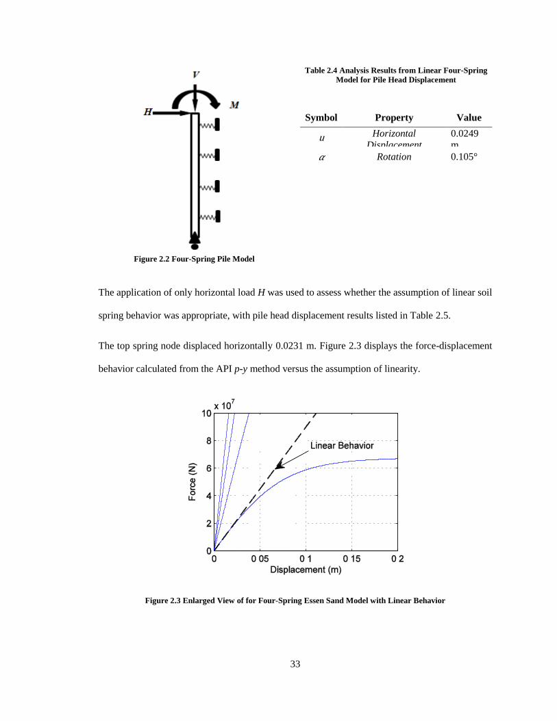
33
Figure 2.2 Four-Spring Pile Model
Table 2.4 Analysis Results from Linear Four-Spring
Model for Pile Head Displacement
Symbol Property Value
u Horizontal
Displacement
0.0249
m
𝛼 Rotation 0.105°
The application of only horizontal load H was used to assess whether the assumption of linear soil
spring behavior was appropriate, with pile head displacement results listed in Table 2.5.
The top spring node displaced horizontally 0.0231 m. Figure 2.3 displays the force-displacement
behavior calculated from the API p-y method versus the assumption of linearity.
Figure 2.3 Enlarged View of for Four-Spring Essen Sand Model with Linear Behavior

34
When linear and nonlinear behavior is compared in Figure 2.3, it is inconclusive as to whether or
not a linear assumption is appropriate. To quantify the error in the assumption of linear behavior,
the nonlinear force-displacement curves were compared to linear spring behavior such that
∑
(2.2)
(2.3)
(2.4)
where LR is the linear soil-pile resistance, NLR is the nonlinear resistance, xk is the distance
between soil springs, x is the depth from the ground surface to the soil spring, y is the horizontal
displacement at the soil spring, and P(x) is the soil-pile resistance per unit length. It should be
noted that the absolute value of the horizontal displacement was considered, as soil springs from
the opposing face of the pile are assumed to behave identically if the pile were to deflect in the
negative-y direction.
Using the displacement values from the linear analysis, linear and nonlinear resistances were
calculated.
Table 2.5 Results from Linear vs. Nonlinear Comparison
Spring y (x10-3
m) LR (x107 N) NLR (x10
7 N) LR-NLR (x10
7 N)
1 14.7 1.32 1.31 0.01
2 3.42 0.924 0.924 0.000
3 0.490 0.220 0.220 0.000
4 0.680 0.428 0.428
0.000
Sum: 0.01 x 10⁷ N

35
The summation of the difference between linear and nonlinear resistance for the linear four-
spring model is about 1 x 10⁵ N (or 100 kN). A convergence study (depicted in Figure 2.4 below)
shows that the error converges at 2.1 x 10⁶ N with 20 soil springs.
Figure 2.4 Number of Springs vs. Linear-Nonlinear
Strength Difference
Figure 2.5 Normalized Error vs. Number of Springs
Compared to the horizontal load of 16 MN, the error is equal to 1.3% of the full load and less
than 1% of the estimated linear resistance. Using the full loading (with horizontal H, vertical V,
and moment M loading), the error in assuming linear behavior increases. When normalized with
respect to the linear resistance, the error is approximately 6%. Figure 2.5 shows the convergence
of the normalized error with the number of soil springs.
From these convergence studies, we can assume that 20 springs should be sufficiently accurate to
model a pile of this length. However, a 20-spring linear analysis with the maximum moment from
Lesny, Paikowsky, & Gurbuz (2007) of 855 MN-m applied yielded a horizontal pile head
displacement of 0.0983 m, which is nearly 10% stiffer than the published value of 0.109 m (using
the p-y method). Consequently, assuming linear soil spring behavior is somewhat unconservative,
and soil spring nonlinearity must be incorporated into the two-dimensional MATLAB model.

36
2.2 Static Nonlinear Analysis
Due to the deficiencies of the static linear analysis, a nonlinear analysis was necessary to model
soil-structure behavior more accurately. This analysis takes into account the nonlinearity of soil
spring behavior, thereby allowing the force-displacement curve of a soil spring to more closely
follow the behavior described by the API method.
Soil nonlinearity was introduced by load-controlled sequence. Initially, a single-spring model
with a rigid pile was used (see Figure 2.6) with a horizontal load H of 2,500 MN applied at the
center (at the same depth as the soil spring). This simple model removed the influence of the pile,
so H could be compared directly to the force-displacement curve from the single soil spring.
Figure 2.6 Single-Spring Model for Nonlinear Analysis
The total load H was divided into even increments, or load steps. The first step was applied and
the displacements were processed using the tangential stiffness of the force-displacement curve.
This tangential stiffness is taken from the derivative of the p-y curve equation with respect to y
and multiplied by the tributary length of the spring,
( (
)
) (2.5)
where y is the compression of the spring at the instant of load application.

37
The nodal coordinates of the pile were subsequently adjusted before another load step was
applied; displacements and tangential stiffnesses were processed similarly. A 10-step analysis is
displayed in Figure 2.7. Note that the nonlinear analysis force-displacement curve stops at the
total load H of 2,500 MN.
Figure 2.7 Example 10-Step Nonlinear Analysis
The results from the nonlinear analysis show that a given amount of force yields a smaller
deflection than the API curve. Due to the fact that each step of the analysis assumes a constant
tangential stiffness, it is inevitable that the analysis results from MATLAB will be slightly stiffer
than from a strict p-y analysis following the API curve (whose tangential stiffness decreases
nonlinearly).
A convergence study using the single-spring model was performed with respect to the difference
between the API method force-displacement curve and the applied load from the nonlinear
analysis, normalized with respect to the applied loading (see Figure 2.8). It was determined that
using a 20-step nonlinear analysis would provide sufficient accuracy without sacrificing

38
computation time. This convergence can also be observed in Figure 2.9, where the full loading
was applied to a 20-spring model.
Figure 2.8 Convergence of Nonlinear Analysis for
Single-Spring Pile Model
Figure 2.9 Convergence of Nonlinear Analysis for
20-Spring Pile Model
Using 20 soil springs and a 20-step nonlinear analysis, the resulting pile head displacements are
as listed in Table 2.7.
Table 2.6 Pile Head Deflections from Nonlinear Analysis
Symbol Value
u 0.0952 m
0.5693°
The results from Table 2.7 were compared and normalized to the force-displacement curves from
the API method with a 1.45% error.
2.3 Conclusions
A code was developed in MATLAB to analyze the response of static laterally-loaded OWT pile
foundations in sand. Initially, linear soil behavior was assumed using 20 soil springs to represent
soil-pile resistance. The resulting pile head displacement was 10% stiffer than the published value

39
by Lesny, Paikowsky & Gurbuz (2007). To improve accuracy, soil nonlinearity was taken into
account by using a force-controlled process. Wind, wave and gravity loads were applied
incrementally (as a horizontal force, vertical force, and overturning moment) to the pile head,
taking into account the change in soil spring stiffness at each load increment application (step).
Lesny, Paikowsky & Gurbuz (2007) designed a pile for the North Sea loading conditions, whose
maximum moment was considered to be 855 MN-m. When this moment was applied to the pile
head (neglecting any other loads), the resulting horizontal displacement was 0.109 m. If these
same North Sea loading conditions are applied to the MATLAB model (using 20 springs and a
20-step load application analysis), the pile head displaces 0.1044 m. Given a discrepancy of
approximately 4% (as compared the 10% error from the linear analysis), we can appropriately
consider this MATLAB model to be calibrated.
It should be noted that the digitization of the API figures (which was necessary in order to
automate the creation of p-y curves) lead to a higher estimation for k as a function of relative
density (20,800 kN/m3, as opposed to 19,000 kN/m
3). For this value of k, the static nonlinear
horizontal displacement is 0.1014 m, which is 7% stiffer than the Lesny, Paikowsky, & Gurbuz
result. This difference is considered acceptable for continued use of automated p-y curves.
40
CHAPTER 3
PILE FOUNDATION RELIABILITY
The reliability index (𝛽) is often used to more concisely express small probabilities of failure. The
probability of failure can be calculated from 𝛽 by
𝛽 (3.1)
where pf is the probability of failure and is the normal cumulative distribution function. Using a
first order reliability method, 𝛽 can be estimated from the mean and standard deviation of the
safety margin, which is a function of limit state. For OWTs, these limit states are divided into two
main categories: ultimate limit states and serviceability limit states.
Typically, 𝛽 for OWTs is 4, which corresponds to pf = 3.1671 x 10⁻⁵
or approximately 1 in 31,574
(Stuyts, Vissers, Cathie, & Jaeck, 2011). Phoon (2008) explains that this value of 𝛽 corresponds
to a 50-year OWT design life and an ultimate limit state. For serviceability limit states, the target
𝛽 is 1.5 (pf = 0.1587), corresponding to a 1-year return period (Phoon, 2008).
Ultimate limit states describe a condition which results in the destructive failure of an OWT,
whereas serviceability limit states merely indicate that the OWT will be unable to function
efficiently and effectively under those conditions. The serviceability limit states commonly used
for OWT pile foundations restrict pile head displacement (u) to 0.2 m horizontally or 0.7° of
rotation (𝛼). Using these criteria for failure, they can be written in terms of the safety margins
(3.2)
𝛼 𝛼 (3.3)
These safety margins are a function of loading, pile bending stiffness, and soil-pile resistance. In
reliability based design of OWTs, both loading and soil are can be considered random.

41
Using beta distributions to characterize variability in friction angle (𝜑’) and a Weibull
distribution for load variability, sensitivity analyses are performed using the two-dimensional
model validated in Chapter 2.
3.1 Soil Variability
Soil variability is spatial, not random. Characterizing spatial soil variability with random
processes transfers soil property uncertainty from epistemic to aleatory, facilitating modeling and
greatly assisting engineers in their ability to use geotechnical data for design.
The normal, or Gaussian, probability distribution is commonly used to model variability in soil
properties, partially because it simplifies calculations. However, non-Gaussian distributions are
useful as many soil properties are bounded by particular ranges (e.g., non-negative values) or are
skewed. Beta, gamma, and lognormal distributions are often used.
Due to the variability of soil properties from site to site (and within a site), Baecher & Christian
(2003) caution that it is neither “easy nor wise to apply typical values of soil property
variability… for a reliability analysis.” The study of pile foundation reliability that proceeds in
this thesis is based upon minimal data, which would be insufficient for design. For a realistic pile
design, site-specific geotechnical data is a necessity. Trends would then be fit to the data, likely
characterized using an autocovariance or autocorrelation function. Pile design would proceed
based upon the findings from this type of data analysis.
Without a detailed site investigated from the North Sea site selected by Lesny, Paikowsky &
Gurbuz (2007), the following reliability analyses are more academic than they are realistic.
However, despite the lack of geotechnical data, sensitivity analyses can be conducted to monitor
the response of 𝛽 with respect to soil property distribution, pile parameters, and loading.
42
Soil properties are assumed to be horizontally homogeneous but vertically heterogeneous.
3.1.2. Variation in Friction Angle
Introducing randomness in 𝜑’ produces a significant effect on API p-y curves, and consequently
soil-pile resistance, of a monopile foundation.
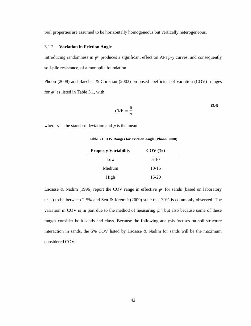
Phoon (2008) and Baecher & Christian (2003) proposed coefficient of variation (COV) ranges
for 𝜑’ as listed in Table 3.1, with
𝜇
𝜎
(3.4)
where 𝜎 is the standard deviation and 𝜇 is the mean.
Table 3.1 COV Ranges for Friction Angle (Phoon, 2008)
Property Variability COV (%)
Low 5-10
Medium 10-15
High 15-20
Lacasse & Nadim (1996) report the COV range in effective 𝜑’ for sands (based on laboratory
tests) to be between 2-5% and Sett & Jeremić (2009) state that 30% is commonly observed. The
variation in COV is in part due to the method of measuring 𝜑’, but also because some of these
ranges consider both sands and clays. Because the following analysis focuses on soil-structure
interaction in sands, the 5% COV listed by Lacasse & Nadim for sands will be the maximum
considered COV.

43
3.1.3. Variation in Relative Density
The relative density of a soil is computed by
(3.5)
where emax is the maximum void ratio for a given soil, emin is the minimum void ratio for the soil,
and e is the in situ void ratio, as measured using a standard laboratory test procedure (e.g., ASTM
D4253 and D4254). Levels of soil density are classified per Table 3.2.
Table 3.2 Density Classification of Soil (Liu & Evett, 2004)
Relative Density Density Classification
<15% Very Loose
15-35% Loose
35-65% Medium Dense
65-85% Dense
85%< Very Dense
Uzielli (2007) reports that the mean relative density (DR) for sand is typically between 30-70%
with a COV ranging from 10-40%.
A proposed relationship between 𝜑’ and DR is listed below (Equation 3.6) for DR more than 35%
(Rankine, Sivakugan, & Cowling, 2006).
𝜑
(3.6)
This relationship was proposed for hydraulic mines in Australia with consistent properties.
Skempton (1986) and Meyerhof (1957) also proposed relationships between the square of DR and

44
𝜑’, but these equations produce significantly lower values for 𝜑’ (by approximately a factor of 2).
Taken out of context, using any of these relationships is probably not appropriate.
API implies a relationship between 𝜑’ and DR as seen in Figure 3.1.
Figure 3.1 Relative Density vs. Friction Angle
This relationship is displayed as piecewise linear, matching the values given for 𝜑’ at the top of
Figure 1.2 with the values at the bottom for DR.
It is evident that the relationship between loose sand (with 𝜑’ less than 30°) is different from
medium dense to dense sands (with a range of 𝜑’ from 30° to 40°). The Essen Sand analyzed in
Chapter 2 (see Table 2.3) displays characteristics of both medium dense and dense sand: If
characterized by relative density, Essen Sand is medium dense; however, if characterized by 𝜑’
(see Figure 1.2), API would consider Essen Sand to be dense. Categorically, a sand which is
classified as either medium dense or dense will not behave as a loose sand.
Because the vast majority of OWT foundation research considers sites with medium dense to
dense sands, the range of 𝜑’ and DR characterizing loose sand will be neglected.
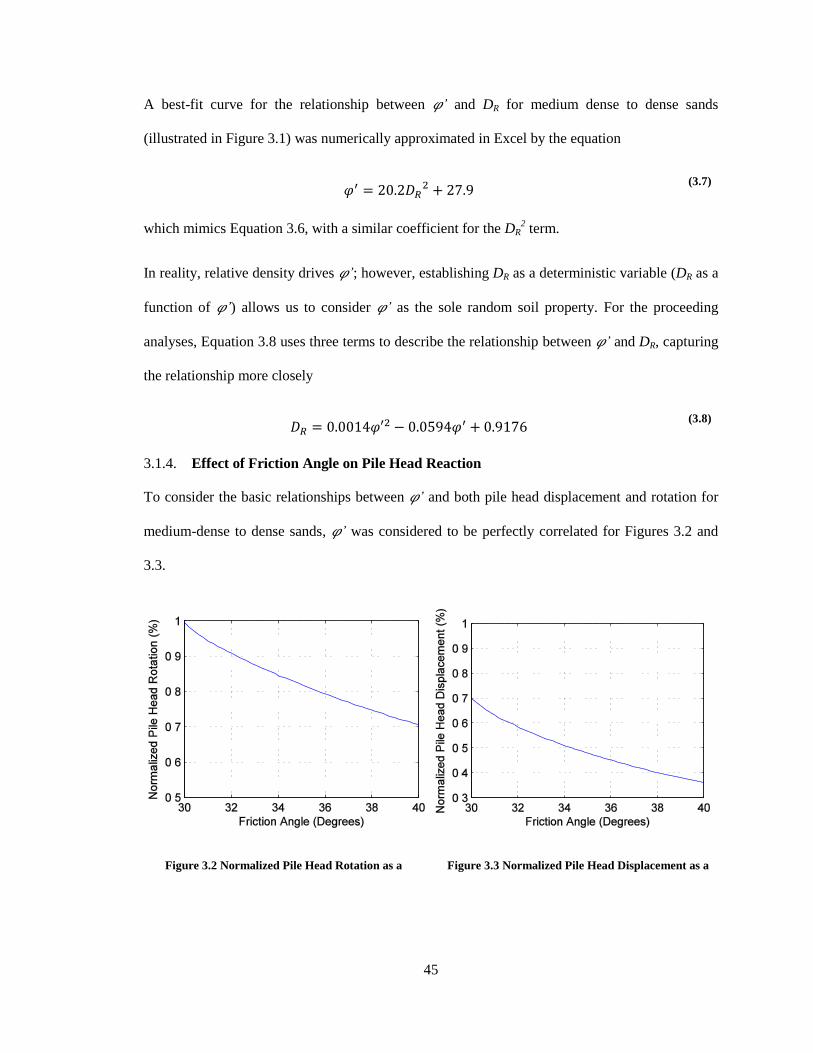
45
A best-fit curve for the relationship between 𝜑’ and DR for medium dense to dense sands
(illustrated in Figure 3.1) was numerically approximated in Excel by the equation
𝜑
(3.7)
which mimics Equation 3.6, with a similar coefficient for the DR2 term.
In reality, relative density drives 𝜑’; however, establishing DR as a deterministic variable (DR as a
function of 𝜑’) allows us to consider 𝜑’ as the sole random soil property. For the proceeding
analyses, Equation 3.8 uses three terms to describe the relationship between 𝜑’ and DR, capturing
the relationship more closely
𝜑 𝜑 (3.8)
3.1.4. Effect of Friction Angle on Pile Head Reaction
To consider the basic relationships between 𝜑’ and both pile head displacement and rotation for
medium-dense to dense sands, 𝜑’ was considered to be perfectly correlated for Figures 3.2 and
3.3.
Figure 3.2 Normalized Pile Head Rotation as a Figure 3.3 Normalized Pile Head Displacement as a

46
Function of Friction Angle Function of Friction Angle
Both figures were normalized with respect to the serviceability limits of 0.7° of rotation and 0.2
m of horizontal displacement.
Note that in Figure 3.2, the maximum rotation (at 𝜑’ = 30°) is just less than the serviceability
limit; in Figure 3.3, the maximum displacement reaches only 70% of the limit. We can expect
that rotation is likely to control reliability given the range of medium-dense to dense sands (𝜑’ =
30°-40°) since the serviceability limit consideration rotation is far closer to being exceeded than
the serviceability limit for horizontal displacement.
3.2 Static Reliability Analysis
This section utilizes the static nonlinear model from Chapter 2, which was adapted to analyze the
reliability of an OWT pile foundation. The applied pile design and loads were those calculated by
Lesny, Paikowsky & Gurbuz (2007).
Beta distributions were used to characterize the random generation of 𝜑’, with a lower bound of
30° and upper bound of 40° (representing the range for medium dense to dense sands). The beta
distribution probability density function (PDF) is characterized by Equation 3.9,
𝜑 |
𝜑 𝜑
(3.9)
where A and B are distribution parameters. By using different values of A and B, an infinite
number of distribution shapes can be achieved.
The second moment properties of the safety margins g1 and g2 (Equations 3.2 and 3.3) were
estimated via Monte Carlo (MC) simulation. The reliability indices (β1 and β2) were then

47
calculated by dividing the mean of the safety margin (μg) by the standard deviation (𝜎g) of the
safety margin (See Equations 3.10 and 3.11 below).
𝛽 𝜇
𝜎 (3.10)
𝛽 𝜇
𝜎 (3.11)
3.2.1 Correlated Friction Angle Variation
Correlation in soil properties is somewhat dependent on soil type and testing method, and
extremely site-dependent (Uzielli, Lacasse, Nadim, & Phoon, 2007).
Without a site investigation, we are unable to model a realistic site; however, we can statistically
model variation of φ’ with a stationary, non-Gaussian translation process model
𝜑 ( 𝜑 | | ) (3.12)
Where F𝜑’ is the cumulative distribution function representing 𝜑’, C𝜑’𝜑’is the covariance matrix
and x1 and x2 are two points along the length of the pile.
Without knowing exactly how 𝜑’ varies vertically along the length of the pile, two limiting cases
were considered: perfect correlation and independent variation (white noise process). In terms of
Equation 3.13, independent variation is when C𝜑’𝜑’ is zero, and the opposing assumption of
perfect correlation is when C𝜑’𝜑’ is one.
A convergence study was performed to determine the minimum number of samples suitable for
estimating 𝛽, considering a site with mean 𝜑’ of 35° and COV of 5% (see Figure 3.4). In the case
of perfectly correlated soil conditions, a random value of 𝜑’ was generated (as characterized by
the PDF in Figure 3.4) per sample and remains constant for the full length of the pile, making 𝜑’

48
constant for all soil springs. For independent variation, the variation of 𝜑’ along the length of the
pile is described by a white noise process with randomly generated values of 𝜑’ (with distribution
described by Figure 3.4) for each soil spring.
Figure 3.4 Beta Probability Density Function, 5% COV
Different estimates of 𝛽 were produced based on a certain number of samples. The rotation
reliability index (𝛽2) controlled per expectation (given Figure 3.2 and 3.3), with 𝛽1 larger than 𝛽2
by a factor of three or more. While the total probability theorem would require us to take into
account both reliability indices, 𝛽1 will be considered negligible and reliability will be assessed
per Equation 3.9.
𝛽 𝛽 (3.13)
In order to determine the number of samples necessary to estimate 𝛽, the standard deviation of
twenty estimations of 𝛽 was calculated for several sample sizes.

49
Figure 3.5 Standard Deviation of Reliability Index vs. Number of Samples Considering Friction Angle Variation
The cases of perfect correlation and independent variation demonstrate very similar behavior in
the convergence studies depicted in Figure 3.5. While both curves show convergence at
approximately 5,000 samples, 10,000 samples are required to produce a consistent estimation of
𝛽 within a tolerance of 0.1.
Proceeding analyses will use 10,000 samples to estimate 𝛽.
The resulting reliability indices of these two cases are shown in Table 3.3.
Table 3.3 Comparison of Results from Correlation Limiting Cases
C𝜑’𝜑’ 𝛍𝜶 𝛔𝛂 𝜷 pf
0 0.576 0.027 4.6 1.0141 x 10⁻⁵
1 0.575 0.033 3.8 2.9195 x 10⁻⁴
It is evident from the discrepancy between the two values of 𝛽 (and consequently probability of
failure, pf) that correlation plays a significant role in the reliability analysis. While both analyses
yielded approximately the same mean pile head rotation, the standard deviation of the response
was higher for the perfectly correlated case. The histograms below (Figures 3.6 and 3.7) illustrate

50
the wider spread of rotations experienced by the pile head when 𝜑’ variation is modeled with
perfect correlation.
Figure 3.6 Histogram of Independent Variation Pile
Head Rotation
Figure 3.7 Histogram of Perfect Correlation Pile Head
Rotation
Consider pile head rotation as a function of 𝜑’ (refer to Figure 3.2): because 𝜇𝜑’ for all
independent variation samples is approximately 35°, the range of pile head rotations in Figure 3.6
is understandably narrower than the range of perfectly correlated samples in Figure 3.7 where 𝜇𝜑’
is less than 35° for approximately 50% of the samples.
Correlation should not be ignored in reliability analyses, as evidenced by the results above.
Proceeding analyses in this thesis will present the limiting cases to gauge the potential range of 𝛽,
but the primary assumption will be perfect correlation of 𝜑’ along the length of pile.
3.2.2 Effect of Friction Angle Variance
The effect of 𝜑’ variance on reliability was examined, considering the medium dense to dense
sand range (30°-40°) and a mean 𝜑’ (𝜇𝜑’) of 35°. Figure 3.8 demonstrates the beta PDFs with
COV values ranging from 2-8% and then 8.25% (see Table 3.4 for distribution parameters). This
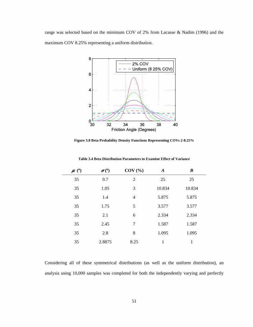
51
range was selected based on the minimum COV of 2% from Lacasse & Nadim (1996) and the
maximum COV 8.25% representing a uniform distribution.
Figure 3.8 Beta Probability Density Functions Representing COVs 2-8.25%
Table 3.4 Beta Distribution Parameters to Examine Effect of Variance
𝝁 (°) 𝝈 (°) COV (%) A B
35 0.7 2 25 25
35 1.05 3 10.834 10.834
35 1.4 4 5.875 5.875
35 1.75 5 3.577 3.577
35 2.1 6 2.334 2.334
35 2.45 7 1.587 1.587
35 2.8 8 1.095 1.095
35 2.8875 8.25 1 1
Considering all of these symmetrical distributions (as well as the uniform distribution), an
analysis using 10,000 samples was completed for both the independently varying and perfectly

52
correlated 𝜑’ cases (see Figure 3.9). As the COV of the beta distribution for 𝜑’ increases, 𝛽
decreases nonlinearly.
Figure 3.9 Reliability Index vs. COV of Friction Angle
If we consider the target 𝛽 to be 4 (in accordance with the 50-year return period used for the
loading), the pile design from Lesny, Paikowsky & Gurbuz (2007) would be considered
appropriate for symmetrically beta distributed soil conditions with 𝜇𝜑’ = 35° and COV between 5
and 6% (bounded by the limiting cases).
The nonlinearity of the reliability problem is emphasized in Figure 3.10, where mean pile head
rotation from 10,000 samples is compared to the COV of the 𝜑’ distribution. While the difference
between minimum and maximum rotations in this range is less than 0.01° (approximately 1.2% of
the maximum rotation), 𝜇𝜑’ is constant at 35°. The output of pile head rotation increases with
variation, despite constant mean input.

53
Figure 3.10 Mean Pile Head Rotation vs. COV of Friction Angle Distribution
3.2.3 Effect of Friction Angle Distribution Shape
One of the main benefits of a beta distribution is in its flexibility, both in distribution shape and
because it can be bounded above and below. We have focused on a particular range of 𝜑’ values
(30°-40°), but there are an infinite number of possibilities for the shape of the beta PDF
representing 𝜑’. The previous section examined the effect of variance on reliability, considering
the mean to be centered at 35°; changing the shape of the PDF will change both the mean and
variance of 𝜑’. The range of beta distribution parameters A and B considered (see Table 3.5)
range from 1 to 3.577, as A = B = 3.577 is equivalent to a symmetrical 5% COV beta distribution.
The type of case examined in Section 3.2.2 can be seen on the diagonal, where the parameters A
and B are of equal value (𝜇𝜑’ = 35°). The values used for A and B were even spaced along the
interval 1 to 3.577.

54
Table 3.5 Mean and Standard Deviation of Friction Angle with Respect to Beta Parameters
B
𝝁, 𝛔 1 1.5154 2.0308 2.5462 3.0616 3.5770
A
1 35.00, 2.89 33.98, 2.61 33.30, 2.34 32.82, 2.11 32.46, 1.91 32.18, 1.75
1.5154 36.03, 2.61 35.00, 2.49 34.28, 2.32 33.73, 2.15 33.31, 1.99 32.98, 1.85
2.0308 36.70, 2.34 35.73, 2.32 35.00, 2.22 34.44, 2.10 33.99, 1.98 33.62, 1.87
2.5462 37.18, 2.11 36.27, 2.15 35.56, 2.10 35.00, 2.03 34.54, 1.94 34.16, 1.85
3.0616 37.54, 1.91 36.69, 1.99 36.01, 1.99 35.46, 1.94 35.00, 1.87 34.61, 1.81
3.5770 37.82, 1.75 37.03, 1.85 36.38, 1.87 35.84, 1.85 35.38, 1.80 35.00, 1.75
Reliability surfaces for the independent variation and perfect correlation cases can be seen in
Figures 3.11 and 3.12, illustrating the increase in 𝛽 as A increases and B decreases.
Figure 3.11 Reliability Surface Considering Beta
Parameters, Independent Variation Case
Figure 3.12 Reliability Surface Considering Beta
Parameters, Perfect Correlation Case
The general shape and behavior of both surfaces is similar, excepting the fact that the independent
variation case rises more steeply into the higher values of 𝛽 than the perfect correlation case.
There is little difference between 𝛽 values when A is 1, but independent variation causes 𝛽 to rise
to higher values than the perfect correlation case when A is 3.577.

55
Contours in Figures 3.13 and 3.14 confirm that as A increases (given a constant value of B), 𝛽
increases more rapidly for the independently varying case than perfectly correlated case.
Figure 3.13 Contour Plot of Reliability Indices with
Respect to Beta Parameters , Independent Variation
Case
Figure 3.14 Contour Plot of Reliability Indices with
Respect to Beta Parameters, Perfect Correlation
Case
At its most dramatic, 𝛽 rises from approximately 2.5 to 7 (seen in Figure 3.13 when B is 1). As B
increases with constant A, 𝛽 decreases slightly; even at the maximum considered value of A
(3.577), this change is from 7 to approximately 4.5.
We can conclude that reliability is more sensitive to variation in the A parameter of the beta
distribution than the B parameter, regardless of correlation case. Knowing that increasing the
COV of 𝜑’ causes a nonlinear decrease in 𝛽 (refer to Figure 3.7), the maximum COV of 5% (per
Lacasse & Nadim, 1996) will yield the most conservative value for 𝛽. A contour plot of 𝜑’ COV
considering various combinations of A and B is illustrated in Figure 3.15.

56
Figure 3.15 Contours of Friction Angle COV with
Respect to Beta Parameters
Figure 3.16 Beta Probability Density Functions with
Approximately 5% COV per Table 3.5
Three points along the 0.05 (5%) contour have been selected to demonstrate how distribution
behavior changes with the selection of A and B (see Table 3.6 and Figure 3.16). As A increases,
the mean of the distribution shifts right, as evidenced in Figure 3.16.
Table 3.6 Beta Parameters Yielding Approximately 5% COV
𝜷
Point A B Independent
Variation
Perfect
Correlation
1 3.75 1.92 5.9 4.8
2 3.577 3.577 4.6 3.8
3 1.5 4.56 2.4 2.0
Analyzing several points along 5% contour line from Figure 3.15, it is evident that as 𝜇𝜑’
increases, 𝛽 increases linearly for both cases (see Figure 3.17).

57
Figure 3.17 Reliability Index vs. Mean Friction Angle
The most conservative distribution of 𝜑’ to assume would be the 5% COV distribution with the
lowest mean value; however, without detailed information from a designated soil site, this choice
is somewhat arbitrary. Given this context, proceeding analyses will assume the simple symmetric
5% COV distribution with 𝜇𝜑’ = 35°. This distribution yields a range of 𝛽 from 3.8 to 4.6
(depending on vertical spatial correlation), considering a loading return period of 50 years and
pile head serviceability limits.
3.2.4 Effect of Pile Parameters
Section 3.2 focused primarily on the effects of soil properties and variation on reliability. In
realistic design scenarios however, pile properties are selected based on the results of a site
investigation. This section focuses on the effect of pile property selection on reliability,
considering pile diameter, wall thickness, and embedment depth. The soil (as previously
discussed in Section 3.2) is characterized by a beta distribution with 𝜇𝜑’ of 35° and 5% COV,
ranging from 30°-40° (see Figure 3.4).

58
A range of diameters from 6 m to 7 m and wall thicknesses from 0.06 m to 0.08 m were analyzed
and are represented by the reliability surfaces in Figures 3.18 and 3.19 (considering the limiting
cases of independent variation and perfect correlation, respectively).
Figure 3.18 Reliability Surface Considering Pile Diameter and Wall Thickness, Independent Variation Case
Figure 3.19 Reliability Surface Considering Pile Diameter and Wall Thickness, Perfect Correlation Case
Predictably, increasing pile diameter and wall thickness raises 𝛽 for both cases. The maximum
and minimum 𝛽 values from the independent variation and perfect correlation cases are listed
below in Table 3.7.

59
Table 3.7 Maximum and Minimum Reliability Indices Considering Pile Diameter and Wall Thickness
Case 𝜷max 𝜷min
Independent Variation 17.6 1.7
Perfect Correlation 16.0 1.4
As pile diameter and wall thickness dictate the moment of inertia (and therefore the bending
capacity) of the pile, contour plots were made of the surfaces in Figures 3.18 and 3.19 to examine
the sensitivity of 𝛽 to bending capacity (see Figures 3.20 and 3.21).
Figure 3.20 Contours of Reliability and Moment of
Inertia, Independent Variation Case
Figure 3.21 Contours of Reliability and Moment of
Inertia, Perfect Correlation Case
The near-parallel reliability and moment of inertia contours of Figures 3.20 and 3.21 indicate that
while soil-pile resistance is a function of pile diameter, the contribution of a pile’s moment of
inertia is the more substantial influence on 𝛽. If the pile diameter effect on soil-pile resistance
were more influential, non-parallel behavior would be exhibited in the contour relationship of
reliability and moment of inertia.

60
The effect of embedment depth on reliability was also analyzed, using the pile cross-section
properties from Lesny, Paikowsky, & Gurbuz (2007). The distance between soil springs (xk) was
held approximately constant for the range of embedment depths considered (30-45 m), dividing
the analyzed depth by the xk determined from the convergence studies for the 38.9 m Lesny,
Paikowsky & Gurbuz pile (1.945 m) and rounding to the nearest whole number of soil springs.
Figure 3.22 illustrates that as embedment depth increases, 𝛽 converges for both cases around 36
m of embedment.
Figure 3.22 Reliability Index vs. Embedment Depth
These results support the previous analysis which considered the Lesny, Paikowsky & Gurbuz
(2007) pile with 38.9 m of embedment.
3.2.5 Load Variation
Similar to cases of soil variation, the absence of site-specific wind and wave data means that the
following sensitivity analysis should be considered academically. The applied horizontal load and
overturning moment would be calculated from site-specific wind and wave distributions, allowing
for a more realistic overview of how load varies.

61
Without this information, a topical study of load variation was conducted assuming constant load
values per Lesny, Paikowsky & Gurbuz (2007) and a constant 𝜑’ of 35° for the full length of the
pile. Table 3.8 compares the influence of the horizontal load H to the overturning moment M
acting at the mudline, with vertical load V applied in both cases. Given the long moment arm that
the tower creates when compared to the fixity at the mudline, the overturning moment is the most
influential factor.
Table 3.8 Loading Influence on Pile Head Response
Pile Head Response Response from H Response from M Full Response
u 0.0238 m 0.0659 m 0.0958 m
% of Full Response 24.8% 68.8% 100%
0.1026° 0.4488° 0.5730°
% of Full Response 17.9% 78.3% 100%
The loads given by Lesny, Paikowsky, & Gurbuz (2007) are calculated from 50-year return
periods of wind and wave loading. It is not economical to design for the highest loads that OWTs
may experience, and as such probability and return periods are used to mitigate the risk of under-
designing while managing the possibility of wasting resources in overdesign.
To consider the sensitivity of an OWT pile foundation to loading, the 50-year return period load
values calculated by Lesny, Paikowsky, & Gurbuz (2007) were treated as mean values with
variation about the mean described by a Weibull distribution. Weibull distributions are commonly
used to model PDFs for long term wind data. Because the vertical loading on an OWT pile
foundation is due to gravity loading, it can be considered deterministic. The mudline loads H and
M are attributed to wind and waves, making them probabilistic loads.

62
Assuming a 5% COV and perfect correlation between the two probabilistic loads (H and M), a
convergence study was performed to determine the appropriate number of samples necessary to
determine 𝛽. In Figure 3.23, soil properties were assumed to be constant (φ’ = 35°).
Figure 3.23 Standard Deviation of Reliability Index vs. Number of Samples Considering Load Variation
Similar to the convergence study regarding the number of samples required to model soil
variation, Figure 3.23 indicates that 10,000 samples are necessary to achieve convergence in the
standard deviation of 𝛽, considering the results of 20 estimates. Considering perfectly correlated
soil properties (𝜑’ = 35°) and 5% COV loading, 𝛽 = 4.1.
The 5% load COV was selected such that the influence of loading and 𝜑’ could be compared.
When depicted next to the convergence studies for 𝜑’, Figure 3.24 demonstrates that the standard
deviation of 𝛽 considering load variation is similar to the studies considering variation in only 𝜑’.

63
Figure 3.24 Comparison of Load and Friction Angle Convergence Figures
As discussed previously however, realistic design situations involve randomness in both the soil
and loading conditions. A convergence study comparison including all of these factors can be
seen below in Figure 3.25.
Figure 3.25 Comparison of Convergence Studies Considering Combinations of Load and Soil Randomness

64
Differentiation between the independent variation and perfect correlation soil convergence studies
were neglected as they have displayed consistent convergence behavior with one another for
every case.
The trend of Figure 3.25 illustrates that the COV of 𝛽 converges in a similar manner despite the
varying sources of randomness. While larger numbers of samples (or an increased number of
estimations) would reduce the noise in the above figure, the general observation of similarity
would remain the same. Table 3.9 below shows the resulting indices per case.
Table 3.9 Reliability Index Results Considering Combinations of Load and Soil Randomness
Sources of Randomness
Soil Case Type Soil Loading Soil & Loading
Independent Variation 4.6 - 3.0
Perfect Correlation 3.8 - 2.8
No Randomness - 4.1 -
Unsurprisingly, taking into account randomness in both soil and loading conditions reduces 𝛽.
3.3 Conclusions
The main objective of this chapter was to determine the effect of soil properties on structural
response. The serviceability requirements (defined by horizontal pile head displacement and pile
head rotation) provided succinct deformation-based limit states that were conducive to reliability
analysis. First-order estimates of the reliability index 𝛽 were dominated by pile head rotation and
thus the probability of horizontal pile head displacement failure was considered negligible.
Analyses were performed to determine the sensitivity of 𝛽 to various parameters. Considering
relative density to be a function of friction angle (𝜑’), epistemic soil randomness was modeled
with the limiting correlation cases of perfect vertical spatial correlation and independent variation

65
(characterized by beta distributions). Using 10,000 samples to estimate the mean and standard
deviation of the safety margin, 𝛽 was calculated using a first order method (see Equations 3.7 and
3.8).
Several conclusions were made from these analyses:
Assuming perfectly correlated soil properties yielded consistently lower 𝛽 values than
assuming independent variation due to variation in pile head response.
As the COV of a symmetric 𝜑’ distribution increases, 𝛽 decreases nonlinearly.
Pile head rotation 𝛼 increased with the COV of a symmetric 𝜑’ distribution, illustrating
the nonlinear aspects of soil-structure interaction.
If the COV of 𝜑’ is assumed constant at 5%, 𝛽 increases linearly with mean friction
angle, 𝜇𝜑’
In realistic design situations, a site investigation is performed at a desired location and the pile
foundation is designed according to available soil properties. Consequently, examining the effect
of soil variation on 𝛽 does not appropriately illustrate the problem from the designer’s viewpoint.
Given an assumed soil profile (where 𝜑’ was characterized by a beta distribution with 𝜇𝜑’=35°
and COV = 5%), the sensitivity of 𝛽 to pile design parameters was assessed. A contour plot
comparing constant values of 𝛽 and moment of inertia (Figures 3.20 and 3.21) revealed that the
bending capacity of the pile was the most influential pile parameter. When 𝛽 was analyzed over a
range of embedment depths, the index value converged at approximately 38 m for the Lesny,
Paikowsky & Gurbuz (2007) example.
Similar to soil variation and pile design parameters, a preliminary sensitivity analysis was
performed for variation in loading conditions. In MATLAB simulations, gravity loads were
considered deterministic while the horizontal loads and overturning moment were modeled as
random and perfectly correlated. The loading values given by Lesny, Paikowsky & Gurbuz

66
(2007) were assumed to be mean values and load variation was characterized by a Weibull
distribution with COV 5% (to mimic the soil variation studies). Comparing the results of the
convergence studies of both soil and load variation (Figure 3.24), it was determined that 𝛽 is
similarly sensitive to load variation as soil variation.
When 5% COV was considered for both load and soil randomness, 𝛽 decreased to 2.8 with the
limiting case of perfect correlation. Despite the reduction in 𝛽, the COV for 20 estimations of 𝛽
was similar to the cases of only load or soil randomness. A more rigorous study of load variation
would include site-specific wind and wave data.
This chapter concludes the sensitivity studies for typical OWT pile foundations.
67
CHAPTER 4
LARGE DIAMETER EFFECTS
When the API equations are extrapolated for OWT pile foundations, theoretical research has
shown that the strength of piles is overestimated for pile diameters exceeding 2 m (Wiemann,
Lesny, & Richwien, 2004). Comparing the analysis results of finite element models to the API p-
y method, Wiemann, Lesny & Richwien (2004) suggest an adjustment factor for the initial
modulus of subgrade
(
)
(4.1)
Where bref is the diameter of a reference pile of 1-2 m and a is 0.6 for medium-dense cohesionless
soils or 0.5 for dense cohesionless soils.
The API method has been considered applicable for pile diameters up to 2 m in diameter, which
is why the adjustment factor reduces the modulus of subgrade based on the relationship of the
designed pile diameter to a reference pile of 1-2 m.
Since there are no particular recommendations regarding what dimension the reference pile
diameter should be, a brief analysis was conducted to examine the behavior of the reliability
index (𝛽) with regard to the choice of reference pile diameter (see Figure 4.1). For this analysis,
the pile parameters and load values given by Lesny, Paikowsky & Gurbuz (2007) were assumed
to be deterministic values and 𝜑’ was characterized by a beta distribution with 𝜇𝜑’ = 35° and 5%
COV.

68
Figure 4.1 Reliability Index vs. Reference Diameter Figure 4.2 Reliability Index vs. Adjusted Initial
Modulus of Subgrade (k*)
In Figure 4.1, 𝛽 demonstrates linearly increasing behavior as bref increases. If k* is utilized in
design, any choice of bref decreases 𝛽 to 1.4-2.8 (depending on bref and soil variation case) from
the previously calculated range of 3.8-4.6 (representing the limiting cases of perfect correlation
and independent variation, respectively). The linearly increase in 𝛽 shown in Figure 4.2 and its
similarity to Figure 4.1 clearly demonstrates the linear relationship between k* and bref,, which
can be seen algebraically in Equation 4.1.
Considering the design life of an OWT, the target 𝛽 is 4; however, the target for a 1-year return
period is 1.5 (Stuyts, Vissers, Cathie, & Jaeck, 2011; Phoon, 2008). It is unclear which target 𝛽
should be applied to this scenario, given that 50-year return periods are used for loading
conditions and serviceability limits are used as a reference for pile head limit state.
4.1 Conclusions
The large diameter-adjusted k* suggested by Wiemann, Lesny & Richwien (2004) reduces the
stiffness of piles by approximately 50-70%, depending on the choice of bref. Consequently, k* also
reduces 𝛽 somewhat substantially. No full-scale tests have been performed to confirm these

69
results, but various researchers have concurred using finite element modeling that the API method
is insufficient for designing piles with diameters in excess of 2 m (Wiemann, Lesny, & Richwien,
2004; Abdel-Rahman & Achmus, 2005). Current design standards do not include any changes to
take into account large-diameter effects.

70
CHAPTER 5
NATURAL FREQUENCY ANALYSIS
Multiple influences must be considered during the dynamic design of OWTs: the frequency
spectra of wind loading, wave loading, and mechanical frequency intervals. Once these input
spectra are determined, a natural frequency is selected and an iterative design methodology is
used to ensure that the foundation and the support structure of the OWT are adequately removed
from a resonant range. In Figure 5.1 below, the frequencies to avoid are demonstrated graphically
for the NREL 5MW Reference Turbine (Petersen, et al., 2010).
Figure 5.1 Structural Design Regime for Offshore Wind Turbines (Petersen, et al., 2010)
Three sea state wave distributions are depicted in Figure 5.1. These sea states are determined by
the mean wind speed, the fetch (the distance over which the wind blows), and the duration of the
71
wind over the open water (NASA, 2000). A sea state is generally described by significant wave
height, which is the average height of the one-third highest waves (NASA, 2000).
The frequencies 1P and 3P represent the mechanical excitation caused by the rotation of one rotor
blade and the combination of all three rotor blades, respectively. OWTs can be designed
according to three different regimes: if f1 is designed to fall below both the 1P and 3P frequencies,
the design is considered “soft-soft”; similarly, if it is designed to fall above both fundamental
frequencies, the design is “stiff-stiff” and in between would be “soft-stiff” (Petersen, et al.,
2010). The majority of OWTs are designed to be soft-stiff (LeBlanc, Houlsby, & Byrne, 2010).
This chapter focuses on solving the characteristic eigenvalue problem for natural frequency. A
deterministic model is developed initially and validated by the published natural frequency values
for the NREL 5MW Reference Turbine. The published model of the NREL 5MW Reference
Turbine is for an onshore design; the substructure and pile are added to the model to determine
the necessary adjustments in wall thickness that would be required to maintain the same first
natural frequency as the Reference Turbine.
After the support structure and foundation wall thicknesses are determined, randomness is
included in the eigenvalue problem. With the inclusion of soil variability, randomness is
introduced into the stiffness matrix, resulting in a distribution of potential frequencies that may
occur.
Moving from a static to dynamic analysis, p-y curves were reduced by 10% per API for cyclic
loading. The effects of damping will be neglected.

72
5.1 Deterministic Eigenvalue Problem
The deterministic eigenvalue problem (Equation 5.1) assumes all input variables are known, non-
random quantities where K is the global stiffness matrix, M is the global mass matrix, and 𝜔 is
the natural frequency (rad/s).
𝜔 (5.1)
Using MATLAB to solve the eigenvalue problem, it was assumed that the steel of the foundation
and support structure is linear, as well as soil-pile resistance.
5.1.1 NREL 5MW Reference Turbine Validation
The model was developed in stages, focusing first on the tower of an onshore turbine,
approximated by a large cantilever. The cantilevered tower was modeled using the properties
listed in Table 5.1 from the NREL 5MW Reference OWT (Jonkman, Butterfield, Musial, &
Scott, 2009).
Table 5.1 Tower and Transition Piece Properties
Property Value
Tower Height 90 m
Tower Base Diameter & Wall Thickness 6 m, 0.035 m
Tower Top Diameter & Wall Thickness 3.87 m, 0.025 m
Modulus of Elasticity 210 GPa
Density of Steel 8,500 kg/m3
Nacelle & Rotor Mass 350,000 kg
Tower Mass 347,460 kg

73
The radius and thickness of the tower were assumed to be linearly tapered from the tower base to
tower top. The density of steel, typically considered 7,850 kg/m3, was increased to 8,500 kg/m
3 to
include paint, bolts, welds and flanges (Jonkman, Butterfield, Musial, & Scott, 2009).
For finite element modeling in MATLAB, a lumped mass matrix was used to model the mass
distribution of the tower, where the element mass matrix (m) is defined per Equation 5.2.
(5.2)
where 𝜌 (kg/m3) is the mass density, A is the cross-sectional area (m
2), and L is the length of the
element (m).
The lumped mass matrix distributes inertial mass to each degree of freedom (DOF) on the
diagonal (see Eq. 5.2 and Figure 5.2) to preserve linear momentum (e.g., the sum of the mass
distributed in the u-direction is equal to the element mass).

74
Figure 5.2 Example Finite Element with Illustrated DOFs
The lumped mass matrix is advantageous not only due to the ease of compilation but also because
it reduces the computational time involved in the solution of the eigenvalue problem. The mass of
the rotor hub and nacelle was added to u1 and v1 of the first element representing the top of the
tower. Hub and nacelle mass was not distributed to the rotational degree of freedom 𝜃1 because it
is fully affixed (and therefore not rotating about the tower).
The stiffness matrix K was formed in an identical manner to the quasi-static model’s stiffness
matrix, though initially the base of the tower was considered fully fixed (at sea level) and the
effect of the sub-sea support structure was neglected.
A convergence study was performed to determine the appropriate element size for modeling the
tower, using the third mode natural frequency (measured in Hz in Figure 5.3).

75
Figure 5.3 Convergence of Third Mode Frequency for NREL 5MW Reference Turbine
An element size of 6 m will be sufficient for modeling the NREL turbine tower.
The natural frequencies for the first three modes are listed in Table 5.2, using the 6 m element
discretization. The tower mass calculated by the MATLAB model was 349,210 kg, which is only
0.5% more than the published value given for the NREL 5MW Reference Turbine.

76
Table 5.2 Dynamic Property Output for the NREL Reference Turbine
Natural Frequency
Mode (Hz) (rad/s) Natural Period (s)
1 0.3162 1.987 3.163
2 2.881 18.10 0.3471
3 7.737 48.61 0.1292
Jonkman, Butterfield, Musial, & Scott (2009) list first mode frequencies ranging from 0.3120 to
0.3240 Hz considering the results fr006Fm FAST and ADAMS for fore-aft and side-to-side first
mode behavior of the turbine. The MATLAB result above is within this range and varies from the
average of the published values (0.3180 Hz) by less than 0.6%, validating the dynamic property
output of the deterministic model.
5.1.2 Deterministic Parametric Studies
Given the results from Section 5.1.1, the NREL 5MW Reference Turbine model developed in
MATLAB can be adapted to include the substructure and foundation (see Figure 5.4).
Figure 5.4 Dimensions of NREL 5MW Reference Turbine in North Sea Conditions
Tower Height, 90 m
Pile Length, 38.9 m
Water Depth, 35 m
Support Structure
Substructure
Foundation

77
Keeping with the parametric studies of Chapter 3, the substructure was added, with a length
equivalent to the mean water depth listed by Lesny, Paikowsky & Gurbuz (2007) of 35.0 m. The
accepted depths for monopile foundations are typically up to 30 m, though some have argued that
they can be used for depths up to 50 m (Lesny & Hinz, 2007; Malhotra, 2010).
The damping effects of water were neglected and the wall thickness of the substructure was
assumed to be constant and equal to the wall thickness at the base of the tower.
Similar to the convergence study for the tower, a study was performed to determine the
appropriate element size for the substructure using the 6 m elements for the tower as previously
determined in Section 5.1.1 (see Figure 5.5).
Figure 5.5 Convergence of Third Mode Natural Frequency for NREL 5MW Reference Turbine, Including
Transition Piece
Three 11.67-m elements were chosen to model the substructure. The added height from the
substructure increased the height of the “on shore” turbine to 125 m, decreasing the natural
frequency to 0.2132 Hz.

78
In the design of the NREL 5MW Reference Turbine, the engineers chose to increase the wall
thicknesses of 0.027 and 0.019 m for the tower base and top (respectively) by 30% in order to
maintain a soft-stiff design regime (Jonkman, Butterfield, Musial, & Scott, 2009). Using a similar
methodology to compare the effects of wall thickness on natural frequency, parametric studies
were performed using percentage increases of the NREL tower wall thickness dimensions and
various substructure wall thicknesses (see Figure 5.6).
Figure 5.6 Effect of Wall Thickness on Natural Frequency, Considering Tower and Substructure
In order to bring the first natural frequency (f1) back up to the minimum 0.3120 Hz, Figure 5.7
shows that the substructure wall thickness would need to be larger than 0.110 m and the tower
wall thickness would need to increase by 70% or more.

79
Figure 5.7 Natural Frequency Contour Plot, in
Reference to Support Structure Wall Thickness
Figure 5.8 Comparison of Support Structure Volume
and Natural Frequency Contours
To optimize the choice of wall thicknesses, the contour plot of f1 from Figure 5.7 was expanded
and compared to contours of constant support structure volume (see Figure 5.8). The volume
contours (using average, mid-height tower properties) indicate that substructure wall thickness
takes precedence over the percentage increase of tower properties. If the substructure wall
thickness is considered to be 0.113 m, a 100% increase is required of the tower wall thicknesses
to be within the range of f1 listed for the NREL 5MW Reference Turbine (see Table 5.3).
Table 5.3 Support Structure Wall Thicknesses, Considering Soil-Level Fixity
Property Value
Substructure Wall Thickness 0.113 m
Tower Base Wall Thickness 0.070 m
Tower Top Wall Thickness 0.049 m
With the properties and discretization of the support structure established, a convergence study
regarding the monopile and soil springs was conducted. The pile is assumed to have the same
diameter and wall thickness as the substructure. Pile properties incorporate the mass of the soil
inside of the pile.

80
In Figure 5.9 below, soil springs were considered to have infinite stiffness.
Figure 5.9 Convergence of First Natural Frequency with Regard to Infinitely Stiff Soil Springs
Per expectation, as the number of infinitely stiff springs increase, so does f1. Using 0.3120 Hz as
the target value, 40 infinitely stiff soil springs (spaced approximately 1 m apart) are necessary to
equate a model including the pile foundation to fixity below the substructure. A convergence
study including real soil stiffness with constant 𝜑’ = 35° can be seen below in Figure 5.10.
Figure 5.10 Convergence of First Natural Frequency with Respect to Soil Springs

81
According to Figure 5.10, f1 converges quickly; using just 5 soil springs is still less than 0.5%
different than the converged value of 0.2646 Hz. Given the results from the reliability analysis of
Chapter 3 however, 20 soil springs will be used to model the pile.
Because the converged value of f1 represents a 15% decrease in stiffness from the NREL 5MW
Reference Turbine, the substructure and tower wall thicknesses were again increased to target the
minimum 0.3120 Hz.
Figures 5.11 and 5.12 below illustrate the effect of substructure wall thickness and percentage
increase of tower wall thickness on f1.
Figure 5.11 Natural Frequency Contour Plot with
Respect to Wall Thickness, Including Monopile
Foundation
Figure 5.12 Comparison of Volume and Natural
Frequency Contours of Support Structure and
Monopile Foundation
While larger wall thickness does increase stiffness, it also adds more mass to the system. At a
certain point, the structural advantage of increasing wall thickness is decreased by the additional
mass, which is demonstrated by the peak in contour curves of Figure 5.12. Using the minimum
volume of steel as the optimum point, the peak of the 0.3120 Hz curve is at a transition wall
thickness of approximately 0.215 m and 30% increase would both increase f1 while minimizing
the amount of steel used. The new wall thickness properties can be found below in Table 5.4.

82
Table 5.4 Support Structure and Foundation Wall Thicknesses
Property Value % Increase from
Soil Fixity Model
Pile & Substructure Wall
Thickness 0.215 m 53%
Tower Base Wall Thickness 0.091 m 30%
Tower Top Wall Thickness 0.064 m 30%
Using the same soil spring discretization of approximately 2 m, f3 is not effectively changed by
embedment length (see Figure 5.13).
Figure 5.13 Effect of Embedment Depth on Third Natural Frequency
While a slight decrease in f3 can be noted from 30 m of embedment to nearly 45 m of embedment,
the change in frequency is negligible – less than 0.3%. This figure confirms that frequency has
converged for a pile embedment depth of 38.9, per Lesny, Paikowsky, & Gurbuz (2007).
The natural frequencies for the first three modes of the NREL 5MW Reference Turbine
MATLAB model (and subsequent two evolutions) are listed in Table 5.5.

83
Table 5.5 Comparison of Unadjusted Dynamic Property Output for the NREL 5MW Reference Turbine,
Including Substructure and Monopile Foundation
Natural Frequency (Hz)
Mode Tower Only
Support Structure
(Tower & Substructure)
Support Structure &
Pile
1 0.3162 0.2132 0.1841
2 2.881 1.560 1.275
3 7.737 4.638 3.776
Avg. % Decrease from Tower Only: 39% 50%
Without increasing the wall thickness from the original NREL parameters, f1 would be reduced
by 50%.
If we use this model to compare the effect of 𝜑’ on f1, Figure 5.14 illustrates that f1 increases
nonlinearly with 𝜑’ for the range of medium dense sand. The difference between the minimum f1
of 0.3120 and the maximum 0.3186 Hz is 5%.
Figure 5.14 First Natural Frequency vs. Friction Angle

84
5.2 Random Eigenvalue Problem
Randomness in soil properties can now be taken into account to produce a distribution of
frequencies that may occur. Including soil variability introduces randomness in the stiffness
matrix portion of the eigenvalue problem, while the mass remains deterministic.
In natural frequency design of OWTs, it is important that the 1P and 3P frequencies associated
with the fundamental frequencies of one and three rotors rotating (respectively, for a three-bladed
turbine) are avoided. In addition to mechanical vibrations, dynamic excitation from wind and
waves frequency spectra must be taken into account as well.
Rather than producing a single value for the frequency associated with each mode, a random K
matrix will produce a distribution of f1; comparing this distribution to the excitation spectra in
Figure 5.1, the probability of resonance can be determined.
As in Chapter 3 regarding pile foundation reliability, both cases of independent variation and
perfect correlation were considered in terms of vertical variability of the soil property 𝜑’.
Distribution of 𝜑’ was considered to be symmetric with 𝜇𝜑’ = 35° and 5% COV. Using MC
simulation to produce estimates of f1, 𝜎f1 converges at approximately 150 samples for both cases
(see Figure 5.15).

85
Figure 5.15 Convergence of Standard Deviation of First Natural Frequency
When estimating f1, the difference between using independent variation or perfect correlation to
model soil variation is small. The similarity between these distributions can be seen in the
outlines of histograms as seen below in Figure 5.16, using 1000 samples to increase the
definition.
Figure 5.16 First Natural Frequency Distribution Comparison of Soil Variation Cases, 1000 Samples

86
The results of the two cases are compared in Table 5.6.
Table 5.6 Frequency Distribution Comparison of Soil Variation Cases
Minimum Maximum 𝝁f1 𝝈f1
Independent Variation 0.3040 0.3177 0.3118 2.715 x 10⁻³
Perfect Correlation 0.3039 0.3178 0.3122 0.0027
The COV of f1 for both of these cases is less than 0.9%. This is unsurprising, as pile foundations
are designed to provide full fixity to the OWT. Less than 28% of these distributions fall outside of
a ±1% change in natural frequency, indicating that while the variation in f1 is small, it is not
small enough to be considered negligible.
With the 1P and 3P frequencies for the NREL 5MW Reference Turbine expanded into bands
(capturing the effect of variable speed rotors), there is no overlap between the frequency
distribution and the given excitation spectra (see Figure 5.17).
Figure 5.17 Offshore Wind Turbine Frequency Compared to Excitation Frequencies (Petersen, et al., 2010)
Distribution
of f1
3P 1P

87
This means that the probability of resonance failure for this OWT turbine design is negligible.
5.3 Conclusions
A natural frequency analysis of the NREL 5MW Reference turbine described by Jonkman,
Butterfield, Musial, & Scott (2009) was performed in MATLAB by solving the characteristic
eigenvalue problem. The resulting first natural frequency (f1) agreed with the FAST and ADAMS
results published, validating the MATLAB modeling process.
The Reference Turbine was based on the design of an onshore wind turbine and thus neglected
any portion of the OWT below the water surface (substructure and foundation). In a deterministic
analysis, the substructure and then pile foundation were added to the MATLAB model, increasing
wall thickness to maintain f1 of 0.3120 Hz (the minimum frequency listed by Jonkman,
Butterfield, Musial & Scott (2009)). Damping and water effects were neglected. The progression
of wall thickness increase can be seen in Table 5.7 below.
Table 5.7 Summary of Wall Thickness Increases
NREL 5MW
Reference
Tower &
Substructure
Tower, Substructure
& Pile
Tower (Bottom/Top) 0.025 / 0.035 m 0.049 / 0.070 m 0.064 / 0.091 m
Substructure & Pile - 0.113 m 0.215 m
Tower wall thickness had to be increased by a factor of nearly 2.6 to maintain the minimum
published frequency by Jonkman, Butterfield, Musial & Scott (2009).
As in Chapters 3 and 4, soil property variability was taken into account by modeling vertical
friction angle (𝜑’) variation. The difference in f1 distribution between independently varying and
perfectly correlated soil properties was negligible (see Figure 5.16). The COV of both f1

88
distributions was less than 0.9%. Despite this small variation, nearly 28% of the distributions fell
outside of ±1% 𝜇f1, indicating that the effect of soil variability should probably not be neglected.
When the full range of f1 was overlaid on the frequency diagram by Petersen et al. (2010), there
was no overlap with the 1P, 3P, wind or wave frequencies, rendering the probability of resonance
failure as negligible.

89
CHAPTER 6
CONCLUSIONS AND RECOMMENDATIONS
Current design standards for offshore wind turbines (OWTs) utilize a deterministic design
procedure that applies partial safety factors to take into account randomness in wind and wave
loading. The goal of this thesis was to analyze the reliability of OWTs with monopile foundations
using probabilistic methods.
Monopile foundations are the most popular design for OWT foundations due to the ease of design
and load application. All standards use the API p-y method to design pile foundations in sand,
which characterizes soil-pile resistance as a series of nonlinear springs along the length of the
pile. Based on research performed by Reese et al. (1975) on 0.6 m-diameter piles, researchers
have noted that there are significant drawbacks when the API p-y method is applied to OWT pile
foundations exceeding 2 m in diameter. Moreover, there is limited understanding of soil-structure
interaction for pile foundations under cyclic conditions; to account for cyclic loading, API RP2A
reduces p-y curves by 10%.
Based on the published results of Lesny, Paikowsky & Gurbuz (2007), a static two-dimensional
model of an OWT monopile foundation was created and validated using MATLAB. With this
base model, epistemic randomness in soil properties was introduced by vertically varying friction
angle (𝜑’). Relative density was related to 𝜑’ based on the figures from API and all soil
properties were considered a function of 𝜑’. Because the beta distribution can be banded above
and below, it was used to model 𝜑’ within the range of medium dense sands (30°-40°). Without
specific soil information from a site, the limiting cases for correlation of 𝜑’ (independent
variation and perfect correlation) between soil springs were considered for all parametric studies.

90
A first order method was implemented to determine the reliability index (𝛽) of the MATLAB
model, using the serviceability limits of the pile head (in terms of displacement and rotation) to
create safety margins. According to Stuyts et al. (2011), the target 𝛽 for serviceability conditions
is 1.5. For an ultimate limit state, Phoon (2008) recommended a 𝛽 of 4. Rotation dominated 𝛽,
and the contribution of failure probability from displacement was neglected. Throughout the soil-
pile interaction studies, assuming perfectly correlated soil properties yielded lower values of 𝛽
than assuming independently varying properties.
Regarding the effect of distribution properties, it was determined that as the COV of a symmetric
(mean friction angle 𝜇𝜑’ = 35°) 𝜑’ distribution increases, 𝛽 decreases nonlinearly. If the COV of
𝜑’ is considered to be the maximum of 5% per Lacasse & Nadim (1996), 𝛽 increased linearly
with 𝜇𝜑’.
Considering that realistic pile design situations are conducted with a given set of soil properties,
the effect of pile diameter, wall thickness, and embedment depth on 𝛽 were studied. In a
parametric study, it was determined that the bending capacity of the pile directly influenced 𝛽,
rendering the effect of pile diameter on API p-y curves negligible by comparison.
In a reliability analysis regarding embedment depth, the pile properties selected by Lesny,
Paikowsky & Gurbuz (2007) were used and analyzed over a range of embedment depths.
Reliability converged around 36 m, which agreed with the designed embedment depth of 38.9 m.
The wind and wave loads acting on OWTs are random. In a preliminary load sensitivity study, the
quasi-static lateral load values from Lesny, Paikowsky, & Gurbuz (2007) were treated as mean
values of Weibull distributions with 5% COV. A more realistic model would include site-specific

91
wind and wave data, from which the applied horizontal load and overturning moment would be
derived.
Comparing the effects of random soil properties and mean load to mean soil properties and
random load, 𝛽 was more sensitive to load variation than soil variation. Considering randomness
in both, the limiting values of 𝛽 was 2.8; however, this study combined 50-year return periods for
loading with serviceability limits which are traditionally associated with a return period of 1 year
(Stuyts, et al., 2011).
The results did not include the effect of large pile diameters. Despite the fact that API p-y curves
do not adequately capture soil-pile resistance for pile diameters beyond 2 m, no design standard
has adopted the adjusted value k* suggested by Wiemann, Lesny & Richwien (2004). If this
adjustment value is incorporated, the limiting value of 𝛽 can be reduced to 1.4.
A natural frequency analysis was conducted by solving the characteristic eigenvalue problem in
MATLAB. Damping was neglected, soil was considered deterministic (𝜑’ = 35°), and all
materials were assumed to be linear. The NREL 5MW Reference Turbine was used to validate
the MATLAB results, and the first natural frequency (f1) agreed with the published results from
FAST and ADAMS by Jonkman, Butterfield, Musial, & Scott (2009). The NREL 5MW
Reference Turbine design did not include details regarding the substructure and pile foundation;
consequently, when these parts of the OWT were added, f1 decreased below the minimum
published value of 3.120 Hz. Using the design methodology mentioned by Jonkman et. al (2009),
the wall thicknesses were increased until f1 agreed with the minimum value.
With the full dynamic OWT model designed, randomness was incorporated in the soil properties.
Using the symmetrical beta distribution previously analyzed, 𝜑’ was assumed to vary vertically
with 𝜇𝜑’ of 35° and 5% COV. Interestingly, considering the limiting correlation cases of

92
independent variation and perfect correlation presented very little difference in the resulting
distribution of f1. The COV of f1 was less than 0.9%, but using a ±1% natural frequency cutoff as
negligible, nearly 72% of the distribution was in the range of negligible variation. Though over a
quarter of the frequencies landed beyond the negligible range, the band of frequencies did not
overlap with the 1P and 3P frequencies of the NREL 5MW Reference Turbine. Additionally, the
distribution of f1 did not coincide with the assumed excitation frequencies from Sea State 3, 6, or
9 wave distributions or wind distribution.
While variation in soil properties did not majorly impact the results of the natural frequency
analysis, it was evident that soil variation was a major influence in quasi-static reliability
analyses. For future studies, a better metric for quantifying the impact of soil variation might
include multiplying the frequency response function of the OWT by the loading spectra of wind
and waves and then integrating for mean square response. Continued study of quasi-static
reliability conditions would best include the results of an offshore soil site investigation, with
which realistic soil properties and variation could be extracted and applied. Alternatively, it
would also be useful to extend the range of soils considered to include all cohesionless and
cohesive soil types.
Steel was considered a completely linear material in this thesis, and the potential for nonlinearity
should be analyzed. Ideally, the issues associated with large diameter piles should also be
monitored by comparing real-time wind and wave data to pile head displacement and rotation on
an installed OWT. Several researchers have analyzed large diameter OWTs using finite element
methods, but no results from large-scale testing or data from previously installed large-diameter
OWTs has been published.

93
For further dynamic analysis, the effects of water on the substructure should be considered. Also,
1% damping should be included for the tower per Jonkman, Butterfield, Musial & Scott (2009).
Large diameter adjustments were not made to the OWT monopile for the natural frequency
analysis and should be taken into account for future studies.
While the simplicity of the monopile foundation option may be advantageous for design and
analysis, this thesis illustrates the sensitivity of pile foundation reliability to soil conditions and
large wall thicknesses required to avoid excitation frequencies. In order to assess the economic
feasibility of monopile OWTs, design, construction, and installation cost estimations would be
required for this design as well as estimations for other OWT foundation options.

94
BIBLIOGRAPHY
(2005). LPILE Plus 5.0. Austin, TX: Ensoft, Inc. Engineering Software.
Abdel-Rahman, K., & Achmus, M. (2005). Finite Element Modelling of Horizontally Loaded
Monopile Foundations for Offshore Wind Energy Converters in Germany. University of
Hannover, Germany, Institute of Soil Mechanics, Foundation Engineering and
Waterpower Engineering. London: Taylor & Francis Group.
ABS. (2010). Guide for Building and Classing Offshore Wind Turbine Installations. Houston,
TX: American Bureau of Shipping.
API. (2005). Recommended Practice for Planning, Designing, and Constructing Fixed Offshore
Platforms - Working Stress Design. Washington, D.C.: American Petroleum Institute.
Ariston, I. K. (2010). Grouted Connections for Offshore Wind Turbines. TUDelft.
Baecher, G. B., & Christian, J. B. (2003). Reliability and Statistics in Geotechnical Engineering.
John Wiley & Sons.
Bir, G., & Jonkman, J. (2008). Modal Dynamics of Large Wind Turbines with Different Support
Structures. ASME 27th International Conference on Offshore Mechanics and Arctic
Engineering. Estoril, Portugal: National Renewable Energy Laboratory.
Bolinger, M., & Wiser, R. (2008). Annual Report on U.S. Wind Power Installation, Cost, and
Performance Trends: 2007. United States Department of Energy.
Bush, E., & Manuel, L. (2009). Foundation Models for Offshore Wind Turbines. Orlando, FL:
American Institute of Aeronautics and Astronautics.
Cordle, A. (2006). Final report for WP4.3: Enhancement of Design Methods and Standards.
Project UpWind.
Day, R. W. (2000). Geotechnical Engineer's Portable Handbook. New York: McGraw-Hill.
de Vries, W. E., & Krolis, V. D. (2004). Effects of Deep Water on Monopile Support Structures
for Offshore Wind Turbines. Delft University of Technology, Duwind, Civil Engineering
and Geosciences, Delft, the Netherlands.
DeGroot, D. J., & Baecher, G. B. (1993, January). Estimating Autocovariance of In-Situ Soil
Properties. Journal of Geotechnical Engineering, 119(1).
Department of Energy. (2010). 20% Wind Energy by 2030. United States Department of Energy.
DNV. (2009). Offshore Standard DNV-OS-J101: Design of Offshore Wind Turbine Structures.
Norway: Det Norske Veritas.

95
Fenton, G. A., & Griffiths, D. V. (2000). Bearing Capacity of Spatially Random Soils. 8th ASCE
Joint Specialty Conference on Probabilistic Mechanics and Structural Reliability. Notre
Dame, IN.
Gipe, P. (2006, June 7). IEC Wind Turbine Classes. Retrieved January 6, 2010, from Wind-
Works: http://www.wind-works.org/articles/IECWindTurbineClasses.html
GL. (2005). Guideline for the Certification of Offshore Wind Turbines. Uetersen, Germany:
Germanischer Lloyd WindEnergie GmbH.
Goldfingle, G. (2010, Spring). Wind Energy: Foundations. European Foundations, pp. 10-12.
Gur, T., Choi, J., Abadie, R. J., & Barrios, A. C. (2009). Assessment of Platform Cognac Using
Instrumentation Data. Offshore Technology Conference. Houston, Texas.
Hamre, L., Khankandi, S. F., Strom, P., & Athanasiu, C. (2011). Lateral Behaviour of Large
Diameter Monopiles at Sheringham Shoal Wind Farm. London: Taylor and Francis
Group.
Houlsby, G. T., & Byrne, B. W. (2005, April). Design Procedures and Installation of Suction
Caissons in Clay and Other Materials. Geotechnical Engineering 158(GE2), 75-82.
IEC 61400-3. (2009). Design Requirements for Offshore Wind Turbines. Internation
Electrotechnical Commission.
Jonkman, J., Butterfield, S., Musial, W., & Scott, G. (2009). Definition of a 5-MW Reference
Wind Turbine for Offshore System Development. Golden, CO: National Renewable
Energy Laboratory.
Jonkman, J., van Dam, J., & Forsyth, T. (2003). Investigation of the IEC Safety Standard for
Small Wind Turbine Design through Modeling and Testing. ASME Wind Energy
Symposium. Reno, NV: National Renewable Energy Laboratory.
Kramer, S. L. (1988). Development of P-Y Curves for Analysis of Laterally Loaded Piles in
Western Washington. Seattle, Wa: Washington State Department of Transportation.
Krolis, V. D., van der Tempel, J., & de Vries, W. (2007). Evaluation of Foundation Design for
Monopile Support Structures for Offshore Wind Turbines. Delft University of
Technology, Offshore Engineering, Delft, the Netherlands.
Lacasse, S., & Nadim, F. (1996). Uncertainties in Characterizing Soil Properties. Uncertainty in
the Geological Environment: From Theory to Practice (pp. 49-75). Madison, WI: ASCE.
LeBlanc, C., Houlsby, G. T., & Byrne, B. W. (2010). Response of Stiff Piles in Sand to Long-
Term Cyclic Lateral Loading. Geotechnique, 2(60), pp. 79-90.
Lesny, K., & Hinz, P. (2007). Investigation of Monopile Behavior under Cyclic Lateral Loading.
6th International Offshore Site Investigation and Geotechnics Conference, (pp. 383-390).
London.
96
Lesny, K., & Wiemann, J. (2005). Finite-Element-Modelling of Large Diameter Monopiles for
Offshore Wind Energy Converters. Institute of Soil Mechanics and Foundation of
Engineering. Essen, Germany: University of Duisburg-Essen.
Lesny, K., Paikowsky, S. G., & Gurbuz, A. (2007). Scale Effects in Lateral Load Response of
Large Diameter Monopiles. Geo-Denver. Denver, CO: American Society of Civil
Engineers.
Liu, C., & Evett, J. B. (2004). Soils and Foundations (6th ed.). Upper Saddle River, NJ: Pearson
Prentice Hall.
Long, J. H., & Vanneste, G. (1994, January). Effects of Cyclic Lateral Loads on Piles in Sand.
Journal of Geotechnical Engineering, 120(No. 1).
Malhotra, S. (2010, August). Supporting the Winds of Change. Civil Engineering, pp. 76-85.
Matlock, H. (1970). Correlations for Design of Laterally Loaded Piles in Soft Clay. Offshore
Technology Conference. Dallas, TX.
Musial, W., & Ram, B. (September 2010). Large-Scale Offshore Wind Power in the United
States: Assessment of Opportunities and Barriers. National Renewable Energy
Laboratory.
NASA. (2000, August 11). NASA-HDBK-1001. National Aeronautics and Space Administration.
NREL. (2009, September 9). Offshore Wind Turbine Foundations - Current & Future Prototypes.
Retrieved January 7, 2011, from OffshoreWind.net:
http://offshorewind.net/Other_Pages/Turbine-Foundations.html
Petersen, B., Pollack, M., Connell, B., Greeley, D., Davis, D., Slavik, C., et al. (2010). Evaluate
the Effect of Turbine Period of Vibration Requirements on Structural Design Parameters:
Technical Report of Findings. Groton, CT: Applied Physical Sciences Corp.
Phoon, K.-K. (2008). Reliability-based Design in Geotechnical Engineering: Computations and
Applications. New York, NY: Taylor and Francis.
Quarton, D. (2005). An Internation Design Standard for Offshore Wind Turbines: IEC 61400-3.
Bristol, UK: Garrad Hassan and Partners, Ltd.
Rankine, K. J., Sivakugan, N., & Cowling, R. (2006). Emplaced Geotechnical Characteristics of
Hydraulic Fills in a Number of Australian Mines. Springer.
Reese, L. C., Cox, W. R., & Koop, F. D. (1975). Field Testing and Analysis of Laterally Loaded
Piles in Stiff Clay. Offshore Technology Conference. Dallas, TX.
Saue, M., Lanford, T. E., & Mortensen, N. (2011). Design of Monopile Foundations in Sand for
Offshore Windfarms. Frontiers in Offshore Geotechnics II (pp. 611-616). Taylor &
Francis Group.

97
Schafer, B. (2010). Personal Communication.
Sett, K., & Jeremic, B. (2009). Forward and Backward Probabilistic Simulations in Geotechnical
Engineering. In M. Iskander, D. F. Laefer, & M. H. Hussein, Geotechnical Special
Publication No. 186: Contemporary Topics in In-Situ Testing, Analysis and Reliability of
Foundations (pp. 332-339). Orlando, FL.
Stancich, R. (2010, September 3). Wind Energy Update. Retrieved January 24, 2011, from What's
New about Gravity Base Foundations for Offshore Wind?:
http://social.windenergyupdate.com/qa/what%E2%80%99s-new-about-gravity-base-
foundations-offshore-wind
Stuyts, B., Vissers, V., Cathie, D. N., & Jaeck, C. (2011). Optimizing Site Investigations and Pile
Design for Wind Farms Using Geostatistical Methods: A Case Study. Frontiers in
Offshore Geotechnics II (pp. 629-633). Taylor & Francis Group.
Thomsen, J. H., Forsberg, T., & Bittner, R. (2007). Offshore Wind Turbine Foundations - The
COWI Experience. 26th International Conference on Offshore Mechanics and Arctic
Engineering. San Diego, CA: ASME.
Toft, H. S., & Sorensen, J. D. (2010). Reliability-Based Design of Wind Turbine Components.
TORQUE 2010: The Science of Making Torque from Wind, (pp. 829-838). Crete, Greece.
Uzielli, M., Lacasse, S., Nadim, F., & Phoon, K. (2007). Soil Variability Analysis for
Geotechnical Practice. London: Taylor & Francis Group.
Van Nostrand Reinhold. (2002). Foundation Engineering Handbook (2nd ed.). (H.-Y. Fang, Ed.)
Norwell, MA: Kluwer Academic Publishers.
Wickremesinghe, D., & Campanella, R. G. (1993). Scale of fluctuation as a descriptor of soil
variability. In Li, & Lo (Eds.). Balkema, Rotterdam: Probabilistic Methods in
Geotechnical Engineering.
Wiemann, J., Lesny, K., & Richwien, W. (2004). Evaluation of Pile Diameter Effects on Soil-Pile
Stiffness. University of Duisburg-Essen, Institute for Soil Mechanics and Foundation
Engineering, Essen, Germany.