Turk J Elec Eng & Comp Sci

(2015) 23: 370 – 380

c⃝ TUBITAK

doi:10.3906/elk-1209-28

Turkish Journal of Electrical Engineering & Computer Sciences

http :// journa l s . tub i tak .gov . t r/e lektr ik/

Research Article

Short-term load forecasting without meteorological data using AI-based

structures

Idil ISIKLI ESENER, Tolga YUKSEL∗, Mehmet KURBANDepartment of Electrical and Electronics Engineering, Bilecik Seyh Edebali University, Bilecik, Turkey

Received: 06.09.2012 • Accepted: 05.03.2013 • Published Online: 23.02.2015 • Printed: 20.03.2015

Abstract: STLF is used in making decisions about economical power generation capacity, fuel purchasing, safety

assessment, and power system planning in order to have economical power conditions. In this study, Turkey’s 24-hour-

ahead load forecasting without meteorological data is studied. ANN, wavelet transform and ANN, wavelet transform

and RBF NN, and EMD and RBF NN structures are used in STLF procedures. Local holidays’ historical load data are

changed into data with normal day characteristics, and the estimation results of these days are not included in error

computation. To obtain more accurate results, a regulation on forecasted loads is proposed. Regulated and unregulated

forecasting error percentages are computed as daily average MAPE and maximum daily MAPE, and compared between

the proposed structures. A simulation is performed for the years 2009–2010 via the user interface created using MATLAB

GUI.

Key words: Short-term load forecasting, artificial neural networks, radial basis function neural networks, wavelet

transform, empirical mode decomposition

1. Introduction

Electric power distribution is based on providing continuous, reliable, and economical power to consumers.

Despite increasing load demand, these principles should not be compromised. Hence, electric power system

planning becomes the most important point to focus on in the scope of energy. As the first step of system

planning, load forecasting should be effective, since it determines the entire planning process. Power system

planning based on load forecasting that is lower than required leads to restriction of energy to consumers, while

planning based on the estimation of excess load results in uneconomical operating conditions [1].

Load forecasting is classified as short-term, mid-term, and long-term load forecasting based on forecasting

time range. Short-term load forecasting (STLF) is defined as hourly through daily forecasting, mid-term load

forecasting is estimation from 1 hour to 1 year, and long-term load forecasting extends from 1 year to more [2].

STLF is used in making decisions for economical power generation capacity, fuel purchasing, safety assessment,

and power system planning in order to have economical power conditions.

The methods developed for load forecasting are generally analyzed in 2 categories, analytical methods

and artificial intelligence methods. Commonly used analytical methods in the literature are time series analysis,

regression methods, similar day method, least square estimation (LES), and wavelet transform (WT). Analytical

methods work well in normal daily conditions, but they cannot give satisfactory results when subject to

meteorological, sociological, or economic changes, or the change in load demand during holidays, since they are

∗Correspondence: tolga.yuksel@bilecik.edu.tr

370

ISIKLI ESENER et al./Turk J Elec Eng & Comp Sci

not updated over time. For this reason, artificial intelligence (AI) methods have gained importance in reducing

estimation errors. Artificial neural networks (ANN), fuzzy logic (FL), support vector machines (SVM), genetic

algorithms (GA), particle swarm optimization (PSO), and ant colony optimization (ACO) based methods are

among these AI methods. In addition to these, hybrid methods consist of more than 1 artificial intelligence

method or analytical method, or 2 together. Furthermore, WT is used as a preprocessing tool for AI-based

forecasting.

Factors that affect load demand must be determined well and considered in forecasting studies in order

to produce effective forecasting. These factors can be defined as consumption region and independent variables

like day of the week, sociological, meteorological, demographic, and economic conditions. Demographic and

economic conditions are generally used in long-term load forecasting studies [3], and temperature data are

mostly used as an independent variable in STLF studies [1,2,4–14]. In addition to temperature data, other

meteorological variables like wind, humidity, and precipitation are used in studies [2,7,9,11,15]. There are also

studies using only historical load data [8,16–20]. STLF studies in the literature mostly focus on regional load

forecasting [1,2,5,6,8,9,11,13,14,17].

In this study, Turkey’s 24-hour-ahead load forecasting for the years 2009–2010 was achieved using Turkey’s

historical load data from 1 December 2008 to 31 December 2010, obtained from TEIAS. By contrast with regional

load forecasting, it is quite difficult to obtain and use an effective temperature dataset for large-scale studies

like countrywide estimations with populations of more than 1 million. Therefore, in this study, load forecasting

without temperature data is attempted for a large country. Four different structures are used in the STLF

procedure: ANN, WT and ANN, WT and RBF NN, empirical mode decomposition (EMD) and RBF NN.

Forecasting error percentages are computed as mean absolute percentage error (MAPE) and compared among

these 4 structures. Simulation is performed via the user interface artificial intelligence for short-term load

forecasting (AI–STLF) created using MATLAB GUI.

This paper is organized as follows. In Section 2, studies in the literature related to short-term forecasting

are summarized. In Section 3, WT, RBF NN, and EMD are explained briefly. Input data selection and

formulations for the study are given in Section 4. In Section 5, the STLF procedure is explained. The network

training procedure is described in Section 6. In Section 7, simulation results are given. Finally, in Section 8, a

comparison of the structures is evaluated.

2. Literature overview

There are many studies related to STLF in the literature. Most of these studies focus on artificial intelligence

methods and hybrid methods. Khotanzad et al. forecasted 24-hour loads for a region in the United States

using 6-month hourly load data with ANN [2]. Temperature and humidity data were used as independent

variables in their study. Azadeh et al. used ANN to forecast 24-hour loads for Iran for the years 2003–2005 [4].

Temperature data was used as an independent variable in the study, and different networks were constructed

for each season. Gontar and Hatziargyriou studied 48-hour-ahead load forecasting for Crete using RBF NN

[8] without independent variables. Dongziao and Jie used day type, load, maximum–minimum temperature,

and precipitation data of 16 September 2009 to forecast 24-hour loads for 17 November 2009 with RBF NN

[7]. Xu et al. forecasted 24-hour-ahead loads for Xi’an, China, using temperature and load data with SVM

[13]. Jain and Satish used temperature data as the independent variable in their study of 24-hour-ahead load

forecasting with SVM [10]. Lu and Zhou used load and weather data with PSO-determined parameters of RBF

NN for 24-hour load forecasting for a province in China [11]. Kim et al. used historical load data of the years

371

ISIKLI ESENER et al./Turk J Elec Eng & Comp Sci

1990–1995 with ANN and FL to forecast hourly loads of specific days of the years 1996–1997 for Korea [21].

Song et al. intended to improve the estimations of that study using 20-year historical load data with the fuzzy

linear regression method [22]. He et al. forecasted 24-hour loads for Hebei, China, for the year 2002, using load,

temperature, humidity, and rainfall data with FL-based ANN [9].

There are few STLF studies using only analytical methods, while these methods are widely used in hybrid

methods. Mu et al. studied 7-day-ahead load forecasting for Hainan, China using the similar day method [12].

The input data were chosen as load data, weather conditions, temperature data, day type, sociological conditions,

and day difference in their study. Nalbant et al. forecasted monthly loads for Kutahya, Turkey, for the years

2005–2009 using LES without an independent variable [17]. Sumer et al. did not use any independent variable

in their study of monthly load forecasting using ARIMA, SARIMA, and regression methods [18]. Ceylan and

Demiroren used temperature and load data of the years 2002–2003 to forecast 24-hour loads of Golbası, Turkey,

with ANN and regression methods [5]. Yalcınoz et al. forecasted month-ahead loads for the years 2001–2004

using historical load data of the years 1991–2001 with ANN back propagation algorithm and moving average

method [20]. Chen et al. forecasted 72-hour loads for Guizhou, China, using LES, SVM, and wavelet transform.

Temperature data were used as the independent variable in their study [6]. Gao and Tsoukalas estimated

24-hour-ahead load demand using only historical load data with neural-wavelet methodology [16]. Pandey et

al. did 24- and 168-hour-ahead load forecasting for a region in Canada using time series analysis and fuzzy

neural networks together [1]. Temperature data were used as an independent variable in their study. Taylor and

McSharry studied 24-hour-ahead load forecasting using ARIMA modeling, AR modeling, principal component

analysis (PCA), and Holt–Winters exponential smoothing [19]. An independent variable was not used in their

study. Chen et al. used the similar day method, wavelet transform, and ANN for 24-hour-ahead load forecasting

[15]. Wind-chill temperature, humidex, cloud cover, precipitation, and wind speed were chosen as independent

variables in their study. Zhu et al. used EMD and SVM together for 24-hour-ahead load forecasting for the day

20 June 2005 for Hubei, China [14]. In their study, historical load data were decomposed into intrinsic mode

functions (IMF). Estimation results were achieved by different SVM models for each temperature data-inserted-

IMF. Information about training data is not clear in their study.

3. Methodology

3.1. Wavelet transform

Wavelet transform is a signal analysis method based on Fourier transform. Continuous wavelet transform

(CWT) was developed as an alternative to Fourier and short-time Fourier transforms to determine the frequency

components of the signal at the desired time range in different-sized areas [23]. CWT is obtained by the

convolution of the signal to be analyzed and the scaled (a) and shifted (b) versions of the mother wavelet

function (Ψ), as shown in Eq. (1).

CWT (a, b) =

∫ ∞

−∞f(t) · 1√

a·Ψ

(t− b

a

)· dt. (1)

Discrete wavelet transform (DWT) is a filter bank that decomposes the signal into its low- and high-frequency

components. Transform continues until the desired level is reached by reducing the sample number to half

at each level. The signal is decomposed into coefficients labeled as approximation (cA) for low-frequency

components, and details (cD) for high-frequency components in the first level of transformation. It then

372

ISIKLI ESENER et al./Turk J Elec Eng & Comp Sci

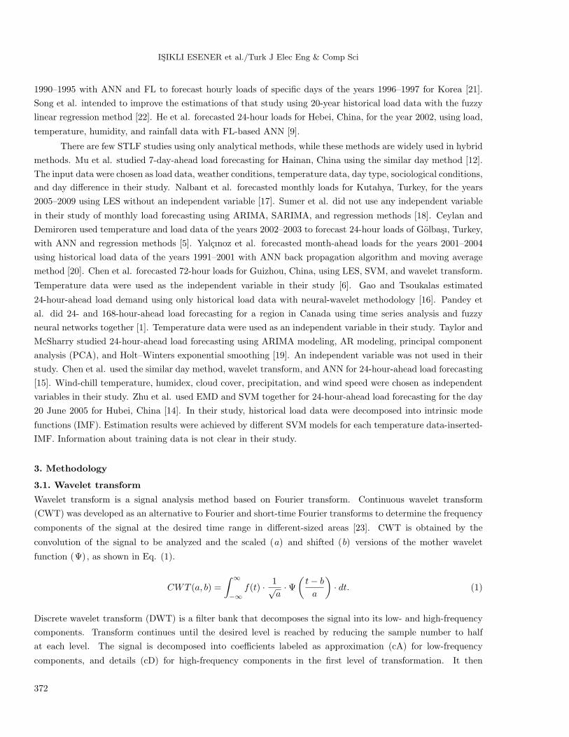
continues decomposing the approximations. Approximation and detail coefficients are computed using Eq.

(2) and Eq. (3), respectively. For a better understanding of DWT, a third-order DWT is shown in Figure 1.

cAj =∞∑−∞

f(n).ϕj,k(n) =∞∑−∞

f(n).1√2j

.ϕ

(n− k.2j

2j

), (2)

cDj =∞∑−∞

f(n).Ψj,k(n) =∞∑−∞

f(n).1√2j

.Ψ

(n− k.2j

2j

). (3)

cA1 cD1

S

cA2 cD2

cD3 cA3

Figure 1. Third-order separation with DWT.

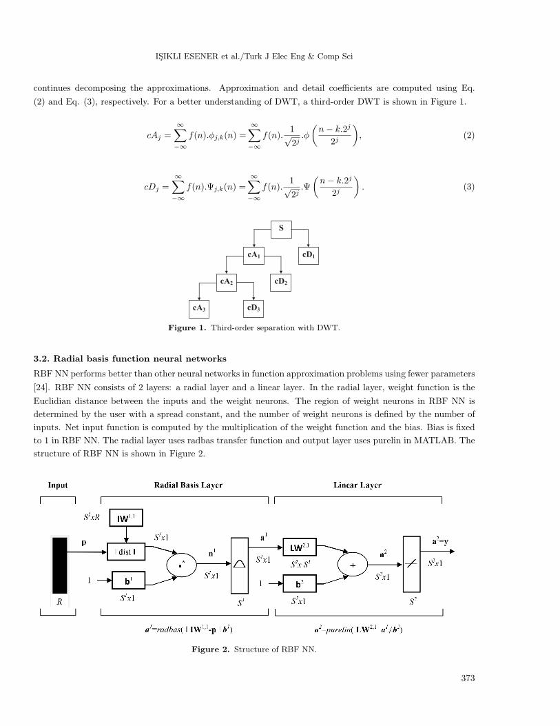
3.2. Radial basis function neural networks

RBF NN performs better than other neural networks in function approximation problems using fewer parameters

[24]. RBF NN consists of 2 layers: a radial layer and a linear layer. In the radial layer, weight function is the

Euclidian distance between the inputs and the weight neurons. The region of weight neurons in RBF NN is

determined by the user with a spread constant, and the number of weight neurons is defined by the number of

inputs. Net input function is computed by the multiplication of the weight function and the bias. Bias is fixed

to 1 in RBF NN. The radial layer uses radbas transfer function and output layer uses purelin in MATLAB. The

structure of RBF NN is shown in Figure 2.

Figure 2. Structure of RBF NN.

373

ISIKLI ESENER et al./Turk J Elec Eng & Comp Sci

3.3. Empirical mode decomposition

As an alternative for wavelets, EMD transform depends on high (detail) and low (trend) frequency decomposition

[25]. This decomposition shows similarities to wavelet transform except in stopping criteria. Decomposition

stops when maximum and minimum points do not exist. EMD is a completely data-driven transform without

analytical analysis. High-frequency components at each level are named intrinsic mode function (IMF).

EMD transform follows the steps of identifying all extremes of x(t), interpolating between minima (resp.

maxima), ending up with some envelope emin(t) (resp. emax (t)), computing the mean (m(t) = (emin (t) +

emax(t)) / 2), extracting the detail (d(t) = x(t) – m(t)), and iterating on the residual m(t) as the new x(t)

[25].

4. Input data selection and formulations

As mentioned in Section 1, load demand changes with meteorological, economic, sociological, and demographic

condition changes. Therefore, independent variables (population; meteorological variables like temperature,

humidity, precipitation; sociological variables including local holidays; and economic variables such as gross

domestic price, imports, exports) must be taken into consideration in load forecasting studies. Temperature

data are frequently used in STLF studies in the literature. In contrast to regional estimations, it is difficult

to obtain effective temperature data for large-scale studies such as countrywide estimations. Consequently,

short-term load forecasting without temperature data is attempted in this study.

Another factor that affects load demand characteristics is local holidays, such as New Year, national, and

regional holidays. Hence, it is quite difficult to form a common structure for local holidays and normal days. For

this reason, it is necessary for local holidays to be substituted with another structure or be removed from the

forecasting study. In this study, local holidays’ historical load data are changed into normal day characteristics

using Eq. (4), and the estimation results of these days are not included in MAPEs.

(data)′

LH =

∣∣∣∣ 7∑d=1

((data)LH − (data)d)+7∑

d=1

((data)LH + (data)d)

∣∣∣∣2

× (data)d (4)

The terms LH and d in Eq. (4) refer to local holiday and day index, respectively.

It is already known that load demand varies seasonally from the studies related to load forecasting

[1,4,8,15,19]. In addition, it is an observable fact that load demand also varies weekly. The analysis of

historical load data clearly shows that load demand deviates with a rate determined by the previous 2 weeks’

load consumptions. Therefore, in order to reduce estimation errors, a regulation for estimating loads is

proposed in this study. Regulated load forecasting is achieved by inserting the deviation rate of weekly load

consumptions into unregulated estimations. Formulations for weekly load consumption, deviation rate of weekly

load consumption, and regulated load forecasting are given in Eq. (5), Eq. (6), and Eq. (7), respectively:

WC =7∑

d=1

24∑h=1

HCdh, (5)

∆WC =WCLW

WCSW, (6)

RLF = URLF + (∆WC − 1)× URLF. (7)

374

ISIKLI ESENER et al./Turk J Elec Eng & Comp Sci

The terms WC, HC, d , h , ∆ WC, WCLW, WCSW, RLF, and URFL in the equations refer to weekly consump-

tion, hourly consumption, day index, hour index, deviation rate of weekly consumption, weekly consumption

of the first week before the forecasted day, weekly consumption of the second week before the forecasted day,

regulated load forecasting, and unregulated load forecasting, respectively.

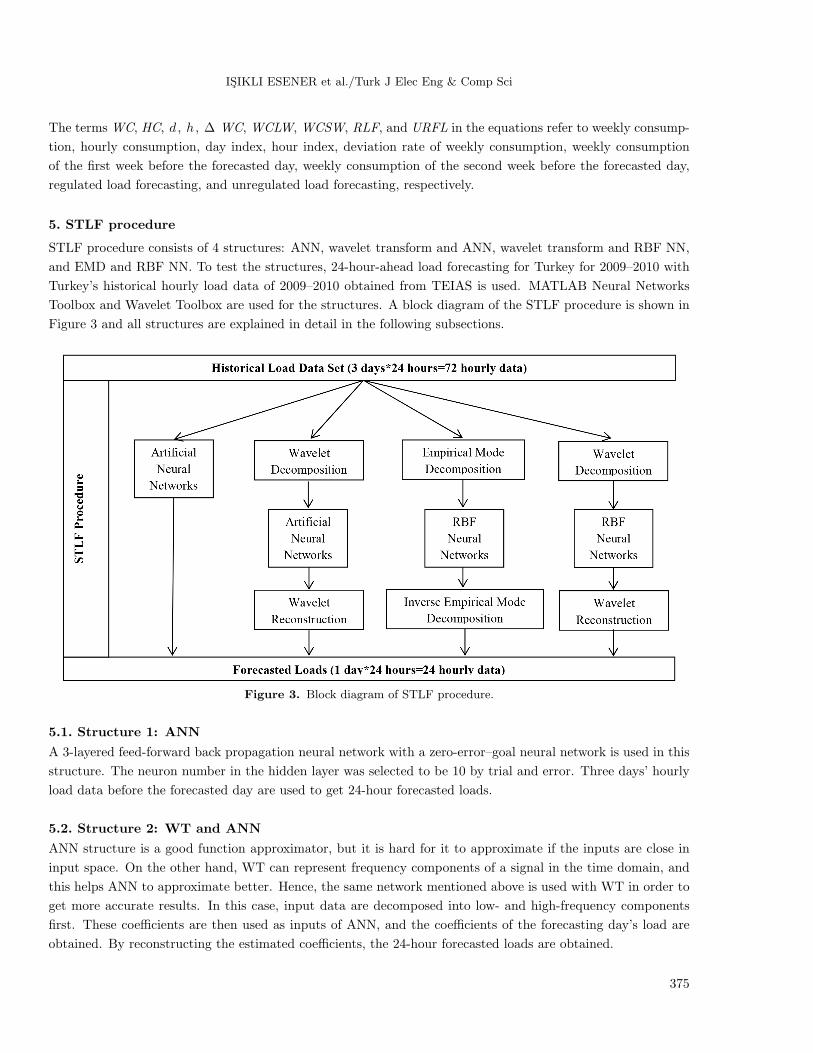
5. STLF procedure

STLF procedure consists of 4 structures: ANN, wavelet transform and ANN, wavelet transform and RBF NN,

and EMD and RBF NN. To test the structures, 24-hour-ahead load forecasting for Turkey for 2009–2010 with

Turkey’s historical hourly load data of 2009–2010 obtained from TEIAS is used. MATLAB Neural Networks

Toolbox and Wavelet Toolbox are used for the structures. A block diagram of the STLF procedure is shown in

Figure 3 and all structures are explained in detail in the following subsections.

Figure 3. Block diagram of STLF procedure.

5.1. Structure 1: ANN

A 3-layered feed-forward back propagation neural network with a zero-error–goal neural network is used in this

structure. The neuron number in the hidden layer was selected to be 10 by trial and error. Three days’ hourly

load data before the forecasted day are used to get 24-hour forecasted loads.

5.2. Structure 2: WT and ANN

ANN structure is a good function approximator, but it is hard for it to approximate if the inputs are close in

input space. On the other hand, WT can represent frequency components of a signal in the time domain, and

this helps ANN to approximate better. Hence, the same network mentioned above is used with WT in order to

get more accurate results. In this case, input data are decomposed into low- and high-frequency components

first. These coefficients are then used as inputs of ANN, and the coefficients of the forecasting day’s load are

obtained. By reconstructing the estimated coefficients, the 24-hour forecasted loads are obtained.

375

ISIKLI ESENER et al./Turk J Elec Eng & Comp Sci

5.3. Structure 3: WT and RBF NN

It is already known that RBF NNs give more accurate results than ANNs for solving nonstationary problems.

Hence, the structure above is reconstructed using RBF NN with spread constant 1 instead of ANN. The

procedure is as described in Section 5.2.

5.4. Structure 4: EMD and RBF NN

In this structure, RBF NN is used with EMD. The input data are decomposed to IMFs, and the RBF neural

network estimates the IMFs of the forecasted day. By summing these estimated IMFs, the 24-hour-ahead

forecasted load is obtained.

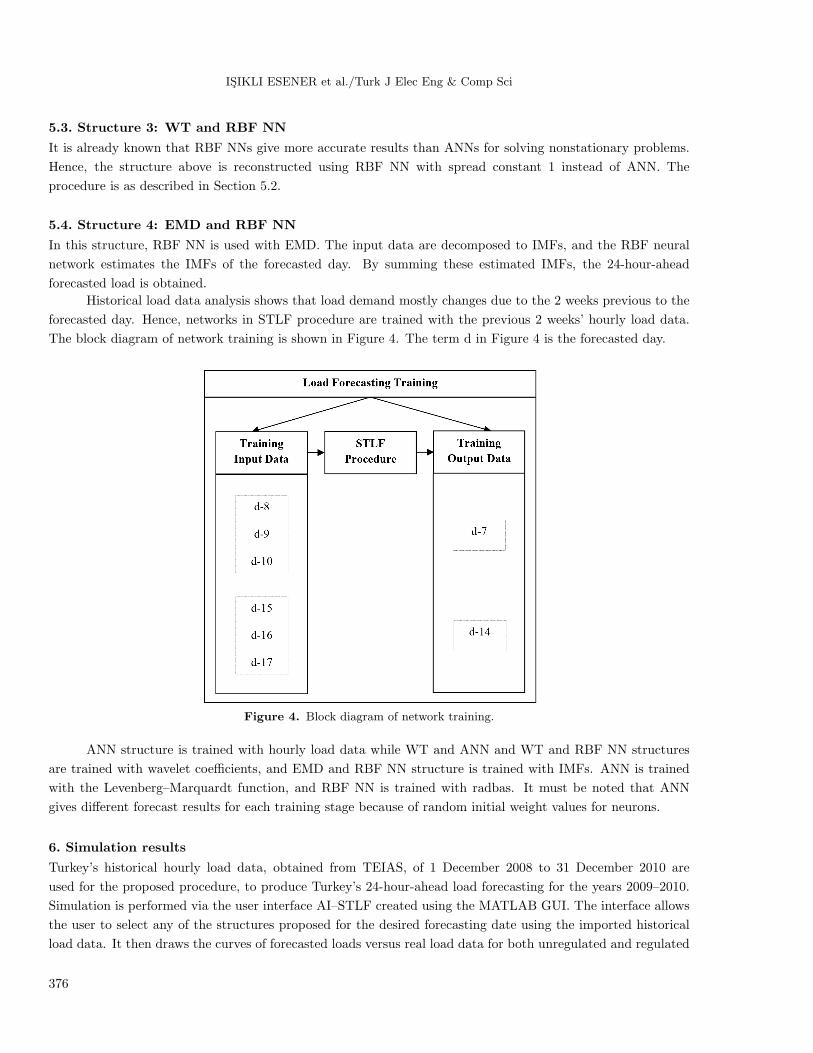
Historical load data analysis shows that load demand mostly changes due to the 2 weeks previous to the

forecasted day. Hence, networks in STLF procedure are trained with the previous 2 weeks’ hourly load data.

The block diagram of network training is shown in Figure 4. The term d in Figure 4 is the forecasted day.

Figure 4. Block diagram of network training.

ANN structure is trained with hourly load data while WT and ANN and WT and RBF NN structures

are trained with wavelet coefficients, and EMD and RBF NN structure is trained with IMFs. ANN is trained

with the Levenberg–Marquardt function, and RBF NN is trained with radbas. It must be noted that ANN

gives different forecast results for each training stage because of random initial weight values for neurons.

6. Simulation results

Turkey’s historical hourly load data, obtained from TEIAS, of 1 December 2008 to 31 December 2010 are

used for the proposed procedure, to produce Turkey’s 24-hour-ahead load forecasting for the years 2009–2010.

Simulation is performed via the user interface AI–STLF created using the MATLAB GUI. The interface allows

the user to select any of the structures proposed for the desired forecasting date using the imported historical

load data. It then draws the curves of forecasted loads versus real load data for both unregulated and regulated

376

ISIKLI ESENER et al./Turk J Elec Eng & Comp Sci

procedures with their MAPE values. Error percentages are computed as MAPE for all estimation results

except for local holidays, and compared between all proposed structures. MAPE values are given as average

daily MAPE and maximum daily MAPE. Daily MAPE and average daily MAPE are computed in Eq. (8) and

Eq. (9), as D in Eq. (9) refers to the number of days without local holidays per year, respectively:

RLF = URLF + (∆WC − 1)× URLF, (8)

RLF = URLF + (∆WC − 1)× URLF. (9)

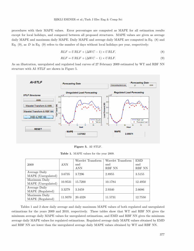
As an illustration, unregulated and regulated load curves of 27 February 2009 estimated by WT and RBF NN

structure with AI–STLF are shown in Figure 5.

Figure 5. AI–STLF.

Table 1. MAPE values for the year 2009.

2009 ANN

Wavelet Transform Wavelet Transform EMDand and andANN RBF NN RBF NN

Average Daily3.6735 3.7296 2.8955 3.5155

MAPE (Unregulated)Maximum Daily

10.9531 15.7200 10.1784 12.4950MAPE (Unregulated)Average Daily

3.3279 3.3459 2.9340 2.6686MAPE (Regulated)Maximum Daily

11.9370 20.4328 11.5731 12.7550MAPE (Regulated)

Tables 1 and 2 show daily average and daily maximum MAPE values of both regulated and unregulated

estimations for the years 2009 and 2010, respectively. These tables show that WT and RBF NN gives the

minimum average daily MAPE values for unregulated estimations, and EMD and RBF NN gives the minimum

average daily MAPE values for regulated estimations. Regulated average daily MAPE values obtained by EMD

and RBF NN are lower than the unregulated average daily MAPE values obtained by WT and RBF NN.

377

ISIKLI ESENER et al./Turk J Elec Eng & Comp Sci

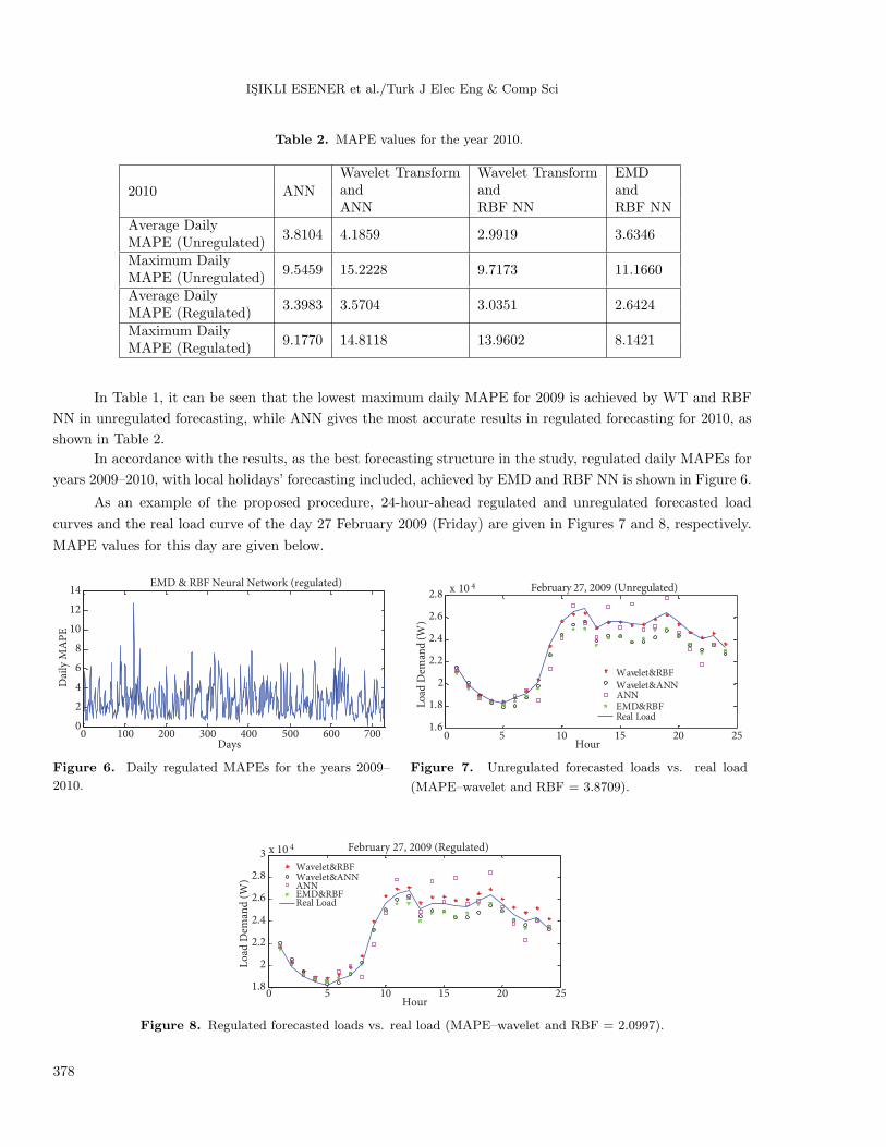
Table 2. MAPE values for the year 2010.

2010 ANN

Wavelet Transform Wavelet Transform EMDand and andANN RBF NN RBF NN

Average Daily3.8104 4.1859 2.9919 3.6346

MAPE (Unregulated)Maximum Daily

9.5459 15.2228 9.7173 11.1660MAPE (Unregulated)Average Daily

3.3983 3.5704 3.0351 2.6424MAPE (Regulated)Maximum Daily

9.1770 14.8118 13.9602 8.1421MAPE (Regulated)

In Table 1, it can be seen that the lowest maximum daily MAPE for 2009 is achieved by WT and RBF

NN in unregulated forecasting, while ANN gives the most accurate results in regulated forecasting for 2010, as

shown in Table 2.

In accordance with the results, as the best forecasting structure in the study, regulated daily MAPEs for

years 2009–2010, with local holidays’ forecasting included, achieved by EMD and RBF NN is shown in Figure 6.

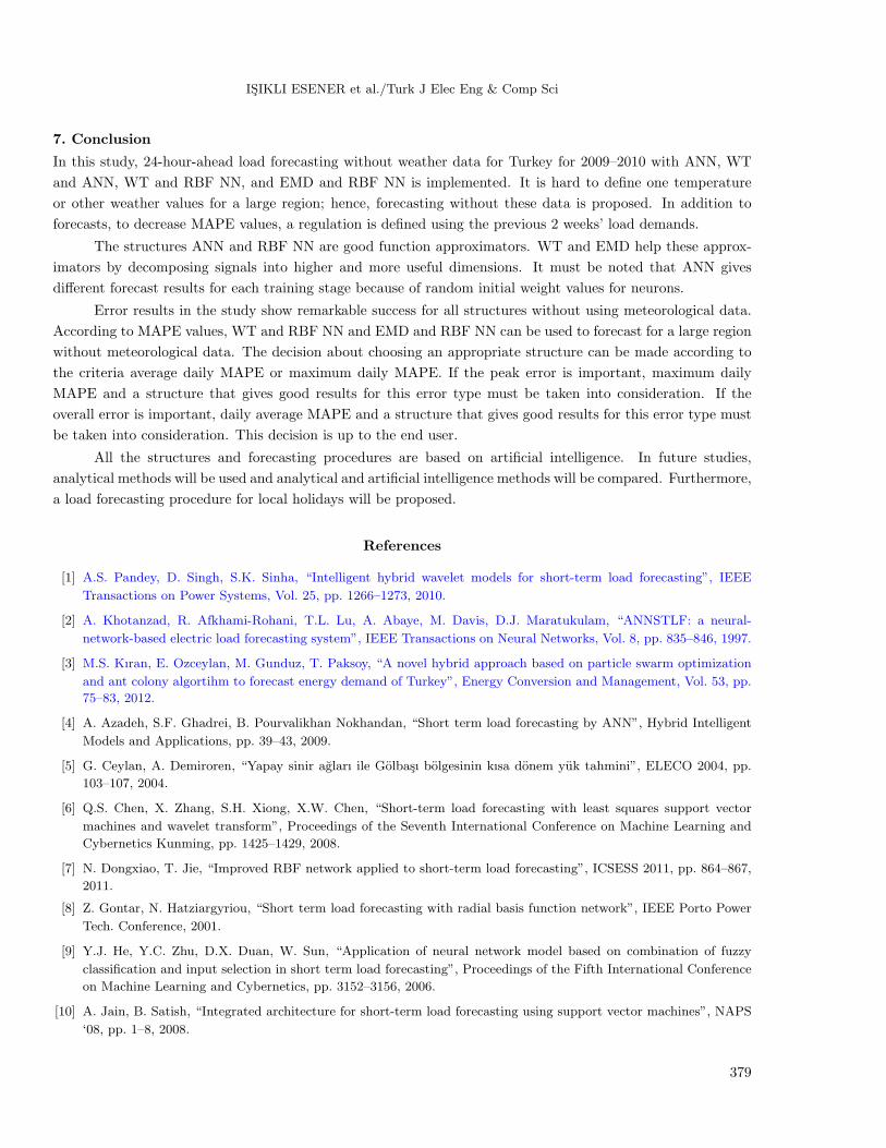
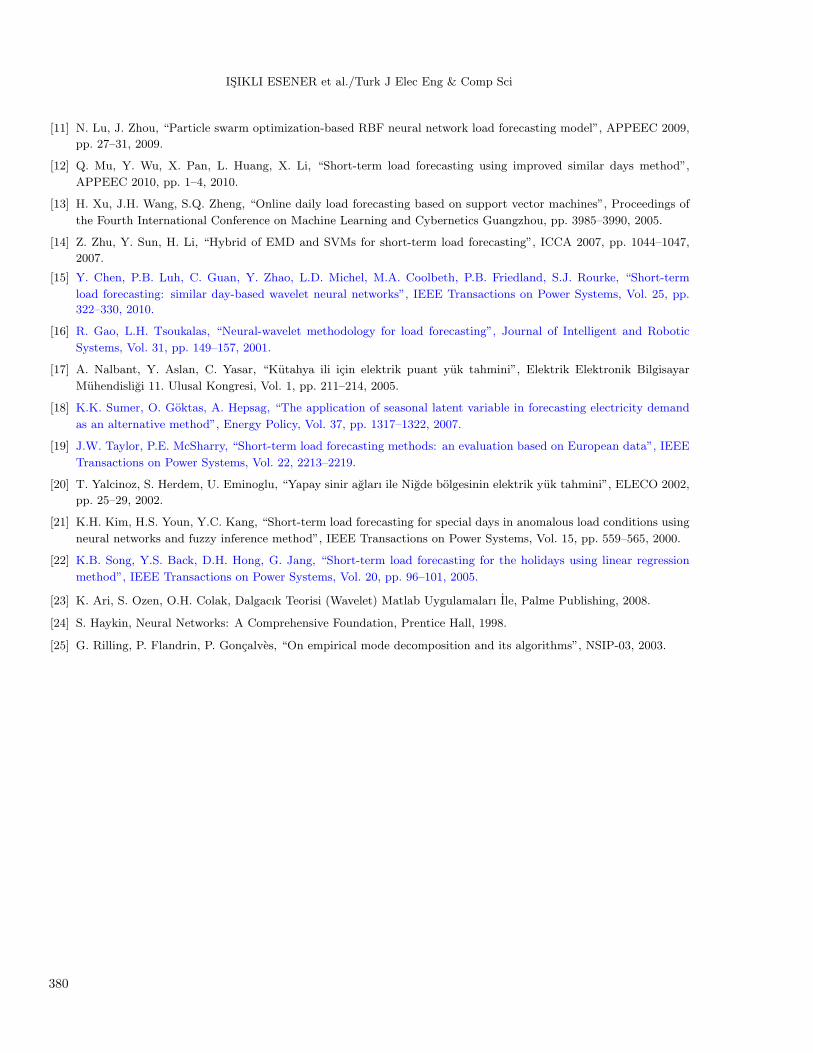
As an example of the proposed procedure, 24-hour-ahead regulated and unregulated forecasted load

curves and the real load curve of the day 27 February 2009 (Friday) are given in Figures 7 and 8, respectively.

MAPE values for this day are given below.

0 100 200 300 400 500 600 7000

2

4

6

8

10

12

14EMD & RBF Neural Network (regulated)

Days

Dai

ly M

AP

E

0 5 10 15 20 251.6

1.8

2

2.2

2.4

2.6

2.8 x 10 4 February 27, 2009 (Unregulated)

Hour

Lo

ad D

eman

d (

W)

Wavelet&RBF

Wavelet&ANNANNEMD&RBFReal Load

Figure 6. Daily regulated MAPEs for the years 2009–

2010.

Figure 7. Unregulated forecasted loads vs. real load

(MAPE–wavelet and RBF = 3.8709).

0 5 10 15 20 251.8

2

2.2

2.4

2.6

2.8

3 x 10 4 February 27, 2009 (Regulated)

Hour

Lo

ad D

eman

d (

W)

Wavelet&RBFWavelet&ANNANNEMD&RBFReal Load

Figure 8. Regulated forecasted loads vs. real load (MAPE–wavelet and RBF = 2.0997).

378

ISIKLI ESENER et al./Turk J Elec Eng & Comp Sci

7. Conclusion

In this study, 24-hour-ahead load forecasting without weather data for Turkey for 2009–2010 with ANN, WT

and ANN, WT and RBF NN, and EMD and RBF NN is implemented. It is hard to define one temperature

or other weather values for a large region; hence, forecasting without these data is proposed. In addition to

forecasts, to decrease MAPE values, a regulation is defined using the previous 2 weeks’ load demands.

The structures ANN and RBF NN are good function approximators. WT and EMD help these approx-

imators by decomposing signals into higher and more useful dimensions. It must be noted that ANN gives

different forecast results for each training stage because of random initial weight values for neurons.

Error results in the study show remarkable success for all structures without using meteorological data.

According to MAPE values, WT and RBF NN and EMD and RBF NN can be used to forecast for a large region

without meteorological data. The decision about choosing an appropriate structure can be made according to

the criteria average daily MAPE or maximum daily MAPE. If the peak error is important, maximum daily

MAPE and a structure that gives good results for this error type must be taken into consideration. If the

overall error is important, daily average MAPE and a structure that gives good results for this error type must

be taken into consideration. This decision is up to the end user.

All the structures and forecasting procedures are based on artificial intelligence. In future studies,

analytical methods will be used and analytical and artificial intelligence methods will be compared. Furthermore,

a load forecasting procedure for local holidays will be proposed.

References

[1] A.S. Pandey, D. Singh, S.K. Sinha, “Intelligent hybrid wavelet models for short-term load forecasting”, IEEE

Transactions on Power Systems, Vol. 25, pp. 1266–1273, 2010.

[2] A. Khotanzad, R. Afkhami-Rohani, T.L. Lu, A. Abaye, M. Davis, D.J. Maratukulam, “ANNSTLF: a neural-

network-based electric load forecasting system”, IEEE Transactions on Neural Networks, Vol. 8, pp. 835–846, 1997.

[3] M.S. Kıran, E. Ozceylan, M. Gunduz, T. Paksoy, “A novel hybrid approach based on particle swarm optimization

and ant colony algortihm to forecast energy demand of Turkey”, Energy Conversion and Management, Vol. 53, pp.

75–83, 2012.

[4] A. Azadeh, S.F. Ghadrei, B. Pourvalikhan Nokhandan, “Short term load forecasting by ANN”, Hybrid Intelligent

Models and Applications, pp. 39–43, 2009.

[5] G. Ceylan, A. Demiroren, “Yapay sinir agları ile Golbası bolgesinin kısa donem yuk tahmini”, ELECO 2004, pp.

103–107, 2004.

[6] Q.S. Chen, X. Zhang, S.H. Xiong, X.W. Chen, “Short-term load forecasting with least squares support vector

machines and wavelet transform”, Proceedings of the Seventh International Conference on Machine Learning and

Cybernetics Kunming, pp. 1425–1429, 2008.

[7] N. Dongxiao, T. Jie, “Improved RBF network applied to short-term load forecasting”, ICSESS 2011, pp. 864–867,

2011.

[8] Z. Gontar, N. Hatziargyriou, “Short term load forecasting with radial basis function network”, IEEE Porto Power

Tech. Conference, 2001.

[9] Y.J. He, Y.C. Zhu, D.X. Duan, W. Sun, “Application of neural network model based on combination of fuzzy

classification and input selection in short term load forecasting”, Proceedings of the Fifth International Conference

on Machine Learning and Cybernetics, pp. 3152–3156, 2006.

[10] A. Jain, B. Satish, “Integrated architecture for short-term load forecasting using support vector machines”, NAPS

‘08, pp. 1–8, 2008.

379

ISIKLI ESENER et al./Turk J Elec Eng & Comp Sci

[11] N. Lu, J. Zhou, “Particle swarm optimization-based RBF neural network load forecasting model”, APPEEC 2009,

pp. 27–31, 2009.

[12] Q. Mu, Y. Wu, X. Pan, L. Huang, X. Li, “Short-term load forecasting using improved similar days method”,

APPEEC 2010, pp. 1–4, 2010.

[13] H. Xu, J.H. Wang, S.Q. Zheng, “Online daily load forecasting based on support vector machines”, Proceedings of

the Fourth International Conference on Machine Learning and Cybernetics Guangzhou, pp. 3985–3990, 2005.

[14] Z. Zhu, Y. Sun, H. Li, “Hybrid of EMD and SVMs for short-term load forecasting”, ICCA 2007, pp. 1044–1047,

2007.

[15] Y. Chen, P.B. Luh, C. Guan, Y. Zhao, L.D. Michel, M.A. Coolbeth, P.B. Friedland, S.J. Rourke, “Short-term

load forecasting: similar day-based wavelet neural networks”, IEEE Transactions on Power Systems, Vol. 25, pp.

322–330, 2010.

[16] R. Gao, L.H. Tsoukalas, “Neural-wavelet methodology for load forecasting”, Journal of Intelligent and Robotic

Systems, Vol. 31, pp. 149–157, 2001.

[17] A. Nalbant, Y. Aslan, C. Yasar, “Kutahya ili icin elektrik puant yuk tahmini”, Elektrik Elektronik Bilgisayar

Muhendisligi 11. Ulusal Kongresi, Vol. 1, pp. 211–214, 2005.

[18] K.K. Sumer, O. Goktas, A. Hepsag, “The application of seasonal latent variable in forecasting electricity demand

as an alternative method”, Energy Policy, Vol. 37, pp. 1317–1322, 2007.

[19] J.W. Taylor, P.E. McSharry, “Short-term load forecasting methods: an evaluation based on European data”, IEEE

Transactions on Power Systems, Vol. 22, 2213–2219.

[20] T. Yalcinoz, S. Herdem, U. Eminoglu, “Yapay sinir agları ile Nigde bolgesinin elektrik yuk tahmini”, ELECO 2002,

pp. 25–29, 2002.

[21] K.H. Kim, H.S. Youn, Y.C. Kang, “Short-term load forecasting for special days in anomalous load conditions using

neural networks and fuzzy inference method”, IEEE Transactions on Power Systems, Vol. 15, pp. 559–565, 2000.

[22] K.B. Song, Y.S. Back, D.H. Hong, G. Jang, “Short-term load forecasting for the holidays using linear regression

method”, IEEE Transactions on Power Systems, Vol. 20, pp. 96–101, 2005.

[23] K. Ari, S. Ozen, O.H. Colak, Dalgacık Teorisi (Wavelet) Matlab Uygulamaları Ile, Palme Publishing, 2008.

[24] S. Haykin, Neural Networks: A Comprehensive Foundation, Prentice Hall, 1998.

[25] G. Rilling, P. Flandrin, P. Goncalves, “On empirical mode decomposition and its algorithms”, NSIP-03, 2003.

380