Embed Size (px)
Citation preview
Comenius University, BratislavaFaculty ofMathematics, Physics and Informatics
Short Distance non-GPS-based Localization ofMobile Devices
Bachelor Thesis
2013
Ladislav Baco
Comenius University, BratislavaFaculty ofMathematics, Physics and Informatics
Short Distance non-GPS-based Localization ofMobile Devices
Bachelor Thesis
Study programme: Computer Science
Study field: 2508 Computer Science, informatics
Department: Department of Computer Science
Supervisor: RNDr. Tomáš Kulich, PhD.
Bratislava, 2013
Ladislav Baco
98071198
Comenius University in BratislavaFaculty of Mathematics, Physics and Informatics
THESIS ASSIGNMENT
Name and Surname: Ladislav BačoStudy programme: Computer Science (Single degree study, bachelor I. deg., full
time form)Field of Study: 9.2.1. Computer Science, InformaticsType of Thesis: Bachelor´s thesisLanguage of Thesis: EnglishSecondary language: Slovak
Title: Short Distance non-GPS-based Localization of Mobile Devices
Aim: Develop mobile application for short distance localization of mobile deviceswithout using GPS system
Supervisor: RNDr. Tomáš Kulich, PhD.Department: FMFI.KI - Department of Computer ScienceVedúci katedry: doc. RNDr. Daniel Olejár, PhD.
Assigned: 16.10.2012
Approved: 24.10.2012 doc. RNDr. Daniel Olejár, PhD.Guarantor of Study Programme
Student Supervisor
98071198
Univerzita Komenského v BratislaveFakulta matematiky, fyziky a informatiky
ZADANIE ZÁVEREČNEJ PRÁCE
Meno a priezvisko študenta: Ladislav BačoŠtudijný program: informatika (Jednoodborové štúdium, bakalársky I. st., denná
forma)Študijný odbor: 9.2.1. informatikaTyp záverečnej práce: bakalárskaJazyk záverečnej práce: anglický
Názov: Lokalizácia mobilných zariadení na malé vzdialenosti nezaložená na GPS
Cieľ: Vytvoriť systém na lokalizáciu mobilných zariadení na malé vzdialenosti bezpoužitia GPS
Vedúci: RNDr. Tomáš Kulich, PhD.Katedra: FMFI.KI - Katedra informatikyVedúci katedry: doc. RNDr. Daniel Olejár, PhD.
Dátum zadania: 16.10.2012
Dátum schválenia: 24.10.2012 doc. RNDr. Daniel Olejár, PhD.garant študijného programu
študent vedúci práce
Acknowledgement
I would like to thank my supervisor RNDr. Tomáš Kulich, PhD. for his help and advices.
v
Abstract
My purpose is to develop an application for short distance non-GPS-based localization of
mobile devices. Localization should work both in exteriors and interiors and should have
minimal prerequisites for its functionality. It also should be precise enought for users to
locate searched objects. Proposed method will be based mainly on the communication over
the WiFi and with sound; sound will be analyzed by Fourier transform. In this thesis I also
performed many experiments and discussed results and the accuracy of the proposed method.
Keywords: localization, smartphone, sound, Fourier transform, Android
vi

Abstrakt
Ciel’om práce je navrhnút’ metódu na lokalizáciu smartfónov na malé vzdialenosti bez pou-
žitia GPS. Lokalizácia by mala fungovat’ v otvorených aj uzavretých priestoroch a mala by
mat’ minimálne požiadavky potrebné pre funkcnost’. Tiež by mala byt’ dostatocne presná,
aby používatel’ vedel urcit’ polohu hl’adaných objektov. Použitá metóda bude využívat’
hlavne na komunikáciu pomocou WiFi a zvuku, pricom analýza zvuku bude založená na
Fourierovej transformácii. Súcast’ou práce je aj vykonanie mnohých experimentov, vyhod-
notenie ich výsledkov a presnosti zvolenej metódy.
K ’lucove slova: lokalizácia, smartfón, zvuk, Fourierova transformácia, Android
vii
Contents
Introduction 1
1 Basic principles and ideas 31.1 Choosing the right approach . . . . . . . . . . . . . . . . . . . . . . . . . 3
1.2 First ideas . . . . . . . . . . . . . . . . . . . . . . . . . . . . . . . . . . . 4
1.2.1 Sound intensity . . . . . . . . . . . . . . . . . . . . . . . . . . . . 4
1.2.2 Audio pings and time . . . . . . . . . . . . . . . . . . . . . . . . . 8
1.3 Description of my concept . . . . . . . . . . . . . . . . . . . . . . . . . . 9
2 Theoretical background 112.1 Clock synchronization . . . . . . . . . . . . . . . . . . . . . . . . . . . . 11
2.1.1 Cristian’s algorithm . . . . . . . . . . . . . . . . . . . . . . . . . . 12
2.1.2 Berkeley algorithm . . . . . . . . . . . . . . . . . . . . . . . . . . 13
2.1.3 Network Time Protocol . . . . . . . . . . . . . . . . . . . . . . . . 14
2.2 Sound analysis . . . . . . . . . . . . . . . . . . . . . . . . . . . . . . . . 14
2.2.1 Fourier series . . . . . . . . . . . . . . . . . . . . . . . . . . . . . 15
2.2.2 Fourier transform . . . . . . . . . . . . . . . . . . . . . . . . . . . 17
2.2.3 Fast Fourier transform . . . . . . . . . . . . . . . . . . . . . . . . 18
2.2.4 Implementation . . . . . . . . . . . . . . . . . . . . . . . . . . . . 18
3 Android application 223.1 Architecture . . . . . . . . . . . . . . . . . . . . . . . . . . . . . . . . . . 22
3.2 Bluetooth and WiFi . . . . . . . . . . . . . . . . . . . . . . . . . . . . . . 24
3.3 Audio recording and playing . . . . . . . . . . . . . . . . . . . . . . . . . 26
3.4 Message loop . . . . . . . . . . . . . . . . . . . . . . . . . . . . . . . . . 28
3.5 Communication protocol of measurement . . . . . . . . . . . . . . . . . . 29
3.6 Experiments and problems . . . . . . . . . . . . . . . . . . . . . . . . . . 30
3.7 Enhanced protocol and results . . . . . . . . . . . . . . . . . . . . . . . . 31
Conclusion 35
viii
List of Figures
1.1 The Circles of Apollonius . . . . . . . . . . . . . . . . . . . . . . . . . . . 5
1.2 Construction of triangle, SSS postulate . . . . . . . . . . . . . . . . . . . . 6
1.3 Principle of audio ping . . . . . . . . . . . . . . . . . . . . . . . . . . . . 9
2.1 Berkeley algorithm for clock synchronization . . . . . . . . . . . . . . . . 13
2.2 Conversion from analog to digital signal . . . . . . . . . . . . . . . . . . . 14
2.3 First partial sums of the Fourier series for a square signal. . . . . . . . . . . 17
2.4 Identical sampling of the different sine signals . . . . . . . . . . . . . . . . 19
2.5 Comparison of my Fourier transform and Minim’s FFT . . . . . . . . . . . 20
3.1 User interface of my application . . . . . . . . . . . . . . . . . . . . . . . 23
3.2 Application schema . . . . . . . . . . . . . . . . . . . . . . . . . . . . . . 23
3.3 The number of measurements and impact on the inaccuracy . . . . . . . . . 32
3.4 The distance between smartphones and impact on the inaccuracy . . . . . . 33
ix
List of Listings
2.1 Fourier transform . . . . . . . . . . . . . . . . . . . . . . . . . . . . . . . 19
2.2 Detection of the audio pings . . . . . . . . . . . . . . . . . . . . . . . . . 21
3.1 Finding out local WiFi IP address . . . . . . . . . . . . . . . . . . . . . . 25
3.2 Client socket . . . . . . . . . . . . . . . . . . . . . . . . . . . . . . . . . 25
3.3 Server socket . . . . . . . . . . . . . . . . . . . . . . . . . . . . . . . . . 25
3.4 Audio recording . . . . . . . . . . . . . . . . . . . . . . . . . . . . . . . . 26
3.5 Audio playing . . . . . . . . . . . . . . . . . . . . . . . . . . . . . . . . . 28
3.6 Thread with message loop . . . . . . . . . . . . . . . . . . . . . . . . . . 28
3.7 Interaction with Handler . . . . . . . . . . . . . . . . . . . . . . . . . . . 29
x
Introduction
Nowadays we can meet new technologies almost everywhere. Many people have note-
books, tablets, smartphones. Especially smartphones bring to us many advantages from
Dream World. Not long ago we can only dream about everyday using of technologies devel-
opped for space race or military purposes.
Today, GPS localization is a common part of our lives. Almost every smartphone and
tablet has GPS receiver ready to use whenever we want. GPS is a great invention, it has
application in various ways, from hiking to navigation around the world. But there are still
some limitations by using this type of localization. GPS does not work well in buildings and
its precision is not as good for civil purposes.
Next I introduce you typical scenarios, in which GPS based localization is inappropriate.
First, we imagine a large music festival with thousands of visitors. When visitor A wants
to meet visitor B, what are his possibilities? He could phone to B, but it is difficult for B
to say the precission location. Naturally, they can arrange a meeting at some well-known
orientation point, but it is not so comfortable. Another possibility is GPS: B shares with A
his coordinates and A goes to B. But this approach has also disadvantage in low precision of
GPS for distinguish visitor B in overloaded stage with visitors.
Another typical scenario is a large conference or exhibition like CES or Campus Party.
When visitor A wants to find visitor B in a large hall with many people, it is not so easy. In
this case GPS is useless because lack of signal in buildings. And phone message to arrange
the meeting is not what we want in this situation.
Assignment. I want to propose a method suitable for short-distance localization of mobile
devices without using Global Positioning System. This method should be suitable for usage
with minimal prerequisites and without any external resources. I also want to determine
accuracy of proposed method.
In this thesis I want to introduce the concept to solve problems in mentioned scenarios and
develop mobile application for Android smartphones which demonstrates practical usability
1
LIST OF LISTINGS 2
of this concept. This includes dealing with minimal prerequisites, theoretical description of
physical principles and algorithms used in my concept, implementation of the theoretical
knowledge and development of demonstrative application with understanding fundamentals
of mobile application programming and practical experiments with discussion and results.
Chapter 1
Basic principles and ideas
1.1 Choosing the right approach
Localization without GPS. . . Okay, but what can we use for determining location, dis-
tances, directions? There are various technologies like a WiFi, Bluetooth, GSM cells, ac-
celerometer, compass and others. In this section I briefly describe their advantages and
disadvantages.
GSM cells. Every GSM cell has a unique ID, so when the phone is connected to the cell,
by knowing this cell’s ID and accessing to database of cell’s IDs, phone knows cell location.
These locations could be used to determine phone’s location, but precision is less then preci-
sion of GPS. Moreover, this approach requires an internet connection (for database access).
WiFi. We have two possible approaches using WiFi. First, we can use strength of access
points and with online database we have similar functionality like with GSM cells with all of
its disadvantages. Second, we can create own access point from our smartphones and with
other spectators we can use the strength of the signal to determine distances between access
points and spectators. That sounds good, but older smartphones do not have the capability
of creating access points. Moreover, Android developer reference [Goo13e] in description
of WifiInfo class says that the API for RSSI (received signal strength indicator) of current
802.11 network is not normalized, but should be. Nice try, but if it is not normalized, how
can I interpreted these values and determine its accuracy?
Accelerometer and compass. Theoretically, accelerometer and compass could be used
for determining changes in location and direction. Then we could compute trajectory of
smartphone’s motion, but it is not what we want. Computing trajectory could be difficult
problem due to inaccuracy of devices, and moreover, we must know some fixed point on the
3
CHAPTER 1. BASIC PRINCIPLES AND IDEAS 4
trajectory for compute relative location to other smartphones.
Bluetooth. Bluetooth is the relatively good choice for short-distance communication be-
tween two devices, but I have no idea how determines locations and/or distances by blue-
tooth. Maybe I could measure the time between transmitting and receiving message, but
because high speed of this interface it is quite impossible for short distances.
Sound. Using a microphone and speaker for receiving and transmitting audio pings can
be a good idea. Speed of sound is not so high and for short distances smartphones could
measure travelling time of the message. Another approach can be based on the intensities of
captured sound.
1.2 First ideas
1.2.1 Sound intensity
Sound intensity is defined as the sound power per unit area. We can imagine a sphere with
an area A and the source of sound with power P in its center, then sound intensity I on this
sphere is I = P/A. If I know the power of the source and I measure sound intensity, I could
compute area and radius of the sphere, which is also the distance between the sound source
and sound detector on sphere.
This theoretical idea is nice, but in application to my situation, the power of sound source
(smartphone’s speaker) is unknown. And neither as this power will be known, it comes
with many problems. For example, when you have your smartphone in a pocket, the sound
is suppressed by clothes. Or when you hold the phone in a hand, you could block out its
loudspeaker and muffle the sound. Similarly, sound damping also depends on position of
device on the desk, e.g. if it is turned upside down or not.
However, theoretical dependencies of intensity and radius could be useful in another ap-
proach. Because area A is proportional to squared sphere’s radius r and intensity is inversely
proportional to the area, sound intensity is inversely proportional to r2, or in other words,
intensity is proportional to r−2.
Imagine that we have three smartphones (with labels A, B, C) in the plane. Phone A plays
sound, phones B and C listen to it and determine its intensity IB, resp. IC. Let the sound
CHAPTER 1. BASIC PRINCIPLES AND IDEAS 5
power of phone A is PA, then next equations hold:
IB =PA
4πr2AB
, IC =PA
4πr2AC
.
Now we can simply determine the ratio of distances rAB and rAC from the ratio of intensities
IB and IC without value of PA:rAB
rAC=
√IC
IB. (1.1)
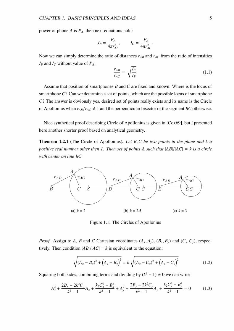
Assume that position of smartphones B and C are fixed and known. Where is the locus of
smartphone C? Can we determine a set of points, which are the possible locus of smartphone
C? The answer is obviously yes, desired set of points really exists and its name is the Circle
of Apollonius when rAB/rAC , 1 and the perpendicular bisector of the segment BC otherwise.
Nice synthetical proof describing Circle of Apollonius is given in [Cox69], but I presented
here another shorter proof based on analytical geometry.
Theorem 1.2.1 (The Circle of Apollonius). Let B,C be two points in the plane and k a
positive real number other then 1. Then set of points A such that |AB|/|AC| = k is a circle
with center on line BC.
A
B C S
rAB rAC
(a) k = 2
A
B C S
rAB rAC
(b) k = 2.5
A
B CS
rAB rAC
(c) k = 3
Figure 1.1: The Circles of Apollonius
Proof. Assign to A, B and C Cartesian coordinates (Ax, Ay), (Bx, By) and (Cx,Cy), respec-
tively. Then condition |AB|/|AC| = k is equivalent to the equation:√(Ax − Bx)2 +
(Ay − By
)2= k
√(Ax −Cx)2 +
(Ay −Cy
)2(1.2)
Squaring both sides, combining terms and dividing by (k2 − 1) , 0 we can write
A2x +
2Bx − 2k2Cx
k2 − 1Ax +
k2C2x − B2
x
k2 − 1+ A2
y +2By − 2k2Cy
k2 − 1Ay +
k2C2y − B2
y
k2 − 1= 0 (1.3)
CHAPTER 1. BASIC PRINCIPLES AND IDEAS 6
We can normalize Cartesian coordinates in the way that By = Cy = 0, so points B and C lie
on x-axis. Then we can rewrite equation 1.3 to next equation:
A2x +
2Bx − 2k2Cx
k2 − 1Ax +
k2C2x − B2
x
k2 − 1+ A2
y = 0 (1.4)
which is equation of a circle with center on x-axis.
On the other side, if point A satisfies 1.4, then also equation 1.2 holds. Thus also condi-
tion |AB|/|AC| = k is satisfied. So point A satisfies ratio condition if and only if lies on the
circle with equation 1.4, resp. 1.3. This circle is called Apollonius circle.
�
However, it is no so accurate if I limited locus of the smartphone A only to the Circle of
Apollonius or bisector of the segment BC. Using this approach, I need at least three fixed
points B,C,D to determine locus of A with better accuracy. Using three fixed points and two
ratios of distances, I have two circles (or bisectors) with up to two intersectors. But having
at least three fixed points is so strong prerequisite.
What about determining all three ratios of distances in case with three smartphones? The-
oretically it is possible with minimal effort. Due to dependency 1.1 only thing the smart-
phones must do, is play some sound and measure sound intensities of other smartphones.
Now I have all three ratios and I can parametrically describe two distances with third dis-
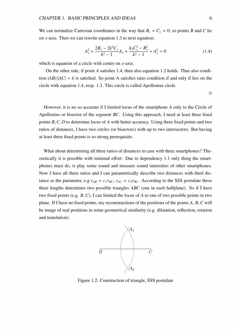
tance as the parameter, e.g rAB = c1rBC, rAC = c2rBC. According to the SSS postulate these
three lengths determines two possible triangles ABC (one in each halfplane). So if I have
two fixed points (e.g. B, C), I can limited the locus of A to one of two possible points in two
plane. If I have no fixed points, my reconstructions of the positions of the points A, B, C will
be image of real positions in some geometrical similarity (e.g. dilatation, reflection, rotation
and translation).
B C
A1
A2
Figure 1.2: Construction of triangle, SSS postulate
CHAPTER 1. BASIC PRINCIPLES AND IDEAS 7
Next, assume that there are n ≥ 3 smartphones in the plane and all ratios of distances
among them are known. With at least three fixed points I can reconstruct real positions of all
the points (with two fixed points we can construct two possible triangles using SSS postulate
as the intersections of two circles, and with third fixed point as the center of third circle we
figure out unique intersection as the locus). Thanks to fixed points I can extract real distances
from ratios. With these lengths and three fixed points it is easy to geometrically construct
positions of the other points, because each point lies on three distinct circles with exactly
one intersection.
With less fixed points, I will not be able to reconstruct the exact real situation, but it is
still not bad: with two fixed points real situation will be one of two possible reconstructions
which are reflected in a line connecting fixed points. And with one fixed point or without
fixed points my reconstruction will be image of the real situation in some geometrical simi-
larity. This is because if I take some real situation and scaled all lengths by factor k, then all
measured intensities will be scaled by factor k2. Thus ratios of the intensities will be same
as before.
Otherwise, in practice there will be smartphones placed into the space, not the plane. What
is the difference? First, the locuses of points will be determined by spheres, not a circles.
And three spheres do not figure out unique intersection(only in special cases). I need at least
four spheres for constructing exactly one intersection as a locus of searched point. Hence if
I want to reconstruct the exact situation with real distances and positions, I will need at least
four fixed points. Without fixed points, my reconstruction will be image of reality in some
shape-preserving transformation in the space.
Soon I realized that in practice I have another problem: sensitivity of the microphone.
Sensitivity of various devices is not the same and if I place two different smartphones in one
place and measured intensity of the sound transmitted by third smartphone, I will get dif-
ferent results. Maybe this trouble can be solved by implementation variable for microphone
sensitivity. . .
Thinking about this problem brings to me another idea. I can describe each device by
four, resp. five numbers: coordinates (2D or 3D), apparent sound power P and microphone
sensitivity S (factor expressing relation between real intensity and measured intensity at
given frequency). If smartphone A = (xA, yA, zA, PA, S A) capture sound from smartphone
B = (xB, yB, zB, PB, S B), measured intensity IA can be described as
IA = S APB
4π((xA − xB)2 + (yA − yB)2 + (zA − zB)2
)
CHAPTER 1. BASIC PRINCIPLES AND IDEAS 8
Thus for n mobiles I have 4n, resp. 5n variables and(
n2
)equations for intensities. With
greater n I have more equations than variables, maybe I could find the unique solution of this
system of the nonlinear equations. Indeed it is not so easy, and moreover, this system does
not have the unique solution. If I double all the powers and half all the sensitivities, I have
another solution of this system. Or if I scaled all the powers, sensitivities and coordinates by
the factor k, all the equations will be satisfied.
I found one attempt of implementation this method with intensities in [Liu10], but it is only
something like an unfinished draft with basic ideas and not describing the transformation of
the intensities to the distances. It is not so encouraging, but this approach may be good with
a couple of prerequisites (e.g. number of the fixed points).
In theory, it seems to be fine, it can correctly reconstruct the real situation with small
amount of the fixed points, or without fixed points it can reconstruct image of the real sit-
uation in some shape-preserving transformation. But in the practice, there always will be
inaccuracy in the measured intensities and computed ratios of the distances. So during my
geometrical construction there will be some kind of errors like not only one intersection of
the circles or spheres. It will be needed to apply some postprocessing and error correction
method. E. g. heuristics that moves each point in the direction of largest error and repeat this
until error will be less than some threshold.
1.2.2 Audio pings and time
The speed of sound is approximately 340 meters per second. It is not so high, thus for short
distances travelling time is measurable. Travelling time is a time delay between transmitting
sound at one place and receiving it at another place. For example this feature is used in active
sonar in submarines, when sonar uses sound transmitter and receiver for emitting sound ping
and listening for echo (reflection). Then computes distance from the time delay between
these two events.
For localization of mobile devices I can use similar principle as active sonar. One smart-
phone creates a short pulse and second smartphone detects it. If both smartphones have
synchronized clocks, then difference in times of these events corresponds to distances be-
tween smartphones. Because one audio ping can be detected by all smartphones within
range, it seems to be quite effective for determining many distances during one round with
only one audio ping. And if all mobiles sequentially send audio pings (or concurrently, but
with distinct frequencies), they can compute distances between all the pair of them.
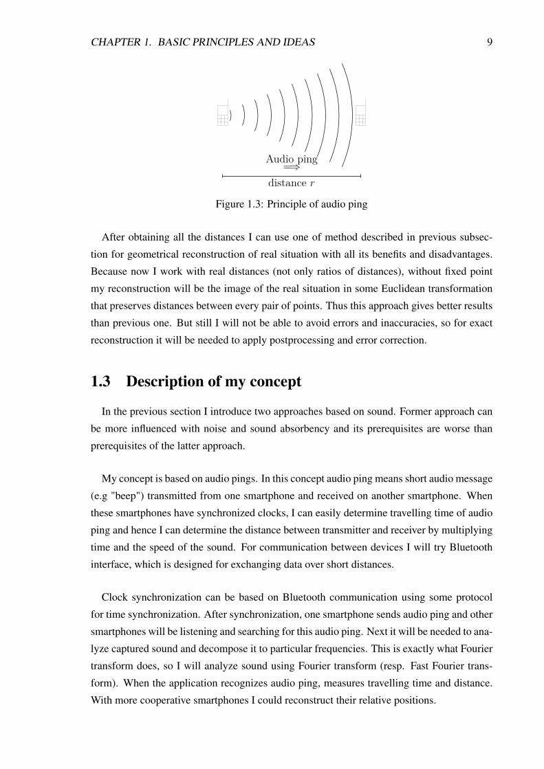
CHAPTER 1. BASIC PRINCIPLES AND IDEAS 9
distance r
Audio ping=⇒
Figure 1.3: Principle of audio ping
After obtaining all the distances I can use one of method described in previous subsec-
tion for geometrical reconstruction of real situation with all its benefits and disadvantages.
Because now I work with real distances (not only ratios of distances), without fixed point
my reconstruction will be the image of the real situation in some Euclidean transformation
that preserves distances between every pair of points. Thus this approach gives better results
than previous one. But still I will not be able to avoid errors and inaccuracies, so for exact
reconstruction it will be needed to apply postprocessing and error correction.
1.3 Description of my concept
In the previous section I introduce two approaches based on sound. Former approach can
be more influenced with noise and sound absorbency and its prerequisites are worse than
prerequisites of the latter approach.
My concept is based on audio pings. In this concept audio ping means short audio message
(e.g "beep") transmitted from one smartphone and received on another smartphone. When
these smartphones have synchronized clocks, I can easily determine travelling time of audio
ping and hence I can determine the distance between transmitter and receiver by multiplying
time and the speed of the sound. For communication between devices I will try Bluetooth
interface, which is designed for exchanging data over short distances.
Clock synchronization can be based on Bluetooth communication using some protocol
for time synchronization. After synchronization, one smartphone sends audio ping and other
smartphones will be listening and searching for this audio ping. Next it will be needed to ana-
lyze captured sound and decompose it to particular frequencies. This is exactly what Fourier
transform does, so I will analyze sound using Fourier transform (resp. Fast Fourier trans-
form). When the application recognizes audio ping, measures travelling time and distance.
With more cooperative smartphones I could reconstruct their relative positions.
CHAPTER 1. BASIC PRINCIPLES AND IDEAS 10
In this thesis I would like to create an application for measuring distances between two
smartphones, but with potential to reconstruct real positions of more smartphones. My ap-
plication will be running on Android smartphones. I choose Android because it is open and
I can easily programming Android applications in Java on desktop with Linux. This is in my
opinion the great advantage of Android, because every developer can create Android applica-
tion and this mobile platform does not prefer any desktop operating system as significantly
as other platforms, e.g. iOS and Windows Phone. Moreover, Google creates quite good
Android developer reference with many tutorials, so it is easy to start with programming
Android applications.
It is a brief description of my initial concept and my decisions about choosing the right
approach and mobile platform. I present further information about clock synchronization,
sound analysis and Android programming in the next chapters.
Chapter 2
Theoretical background
2.1 Clock synchronization
In my concept all the participating smartphones must have the synchronized clocks. Not
necessarily all devices must share the correct UTC time, but every clock should be adjusted
to same time (e.g. local time of one smartphone, average time of the clocks of the smart-
phones,. . . ). Well, time will never be the exactly same, there will be always inaccuracy, but
this inacuraccy has to be less than a few milliseconds because with greater inaccuracy in the
time there will be greater inaccuracy in the evaluate distance. With sound speed approxi-
mately 340 meters per second the time inacuraccy of few milliseconds is acceptable.
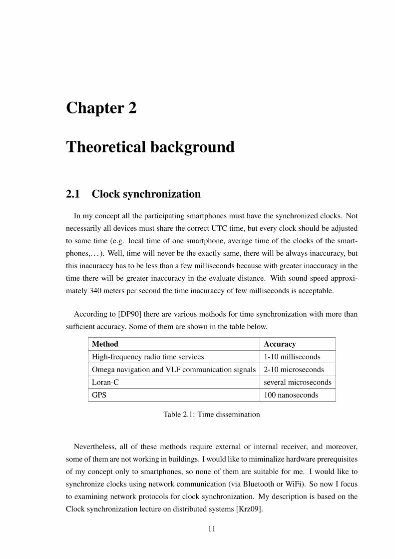
According to [DP90] there are various methods for time synchronization with more than
sufficient accuracy. Some of them are shown in the table below.
Method AccuracyHigh-frequency radio time services 1-10 milliseconds
Omega navigation and VLF communication signals 2-10 microseconds
Loran-C several microseconds
GPS 100 nanoseconds
Table 2.1: Time dissemination
Nevertheless, all of these methods require external or internal receiver, and moreover,
some of them are not working in buildings. I would like to miminalize hardware prerequisites
of my concept only to smartphones, so none of them are suitable for me. I would like to
synchronize clocks using network communication (via Bluetooth or WiFi). So now I focus
to examining network protocols for clock synchronization. My description is based on the
Clock synchronization lecture on distributed systems [Krz09].
11
CHAPTER 2. THEORETICAL BACKGROUND 12
2.1.1 Cristian’s algorithm
First idea about clock synchronization between two devices A and B is simple. A sends
the message to B with timestamp T of the A’s clock and B sets its clock to time T . However,
this is not very reliable due to network delays.
Cristian’s algorithm offers better approach and attempts to compensate these delays. It
measures travelling time of message sending from A to B and back from B to A with local
clock of A. It is expected that network delays in each direction will be almost the same.
This is usually true for Ethernet networks, but 3G networks have different download and
upload speed. However, we can assume that A and B are two identical devices with identical
network connection so it does not matter which of downlink or uplink is a bottleneck, this
is same for both directions of communication. Vecause of our expectation, we assume that
device B measured its time approximately in the middle of time interval between sending
and receiving time. So how exactly Cristian’s algorithm works, if A wants to set the local
clock to time of B’s clock?
1. A sends a request to B at the local system time T0
2. B receives requests and sends to A response with its own local timestamp T
3. A receives B’s response at the local system time T1
4. A sets its own clock to time T + T1−T02
Let the Tmin is the minimum travelling time for sending and receiving messages between
A and B (either direction). Then for timestamp T holds inequality T0 + Tmin ≤ T ≤ T1 −
Tmin. The width of this interval is T1 − T0 − 2Tmin, so the accuracy of Cristian’s algorithm
is
±
∣∣∣∣∣T1 − T0
2− Tmin
∣∣∣∣∣ .Accuracy highly depends on system loads and it varies from a few milliseconds to hun-
dreds of milliseconds. However, we could repeat Cristian’s algorithm several times and use
the one with minimal difference T1 −T0. Thus this is the way how we can improve accuracy.
Also if we know the interrupt handling time of B needed for processing request, we could
improve accuracy even more.
The problem of Cristian’s algorithm is the unavailability of the clock synchronization due
to server failure. Nevertheless, in case of my application this is not a problem, because I do
not have only one server. Instead, I my application the server could be dynamically elected
or simply the server could be the same device, which start the location query.
CHAPTER 2. THEORETICAL BACKGROUND 13
2.1.2 Berkeley algorithm
The Berkeley algorithm for clock synchronization is designed for networks without pre-
cise time source. The basic idea of this algorithm is obtaining average time from all par-
ticipating nodes and synchronizing them to this average time. In contrast with Cristian’s
algorithm in this algorithm server (or master node) synchronizes itself to the average time of
clients.
One of the machines in the network is elected to be a master, other machines are slaves.
Master periodically asks slaves for their time (for example by Cristian’s algorithm due to
network delays). In one round master obtains times from all slaves, computes average time
(including its own time) and sends to slaves time difference between this average and their
local times. Using offsets instead of average time is better, because it minimizes inaccuracies
caused by network other delays.
The Berkeley algorithm hopes that the average time of the all participants helps to min-
imize and cancels out the inaccuracies of single clock, e. g. running faster or slower than
precise time source. Moreover, clients with great deviation can be ignored in computing the
average, which can minimize inaccuracies even better.
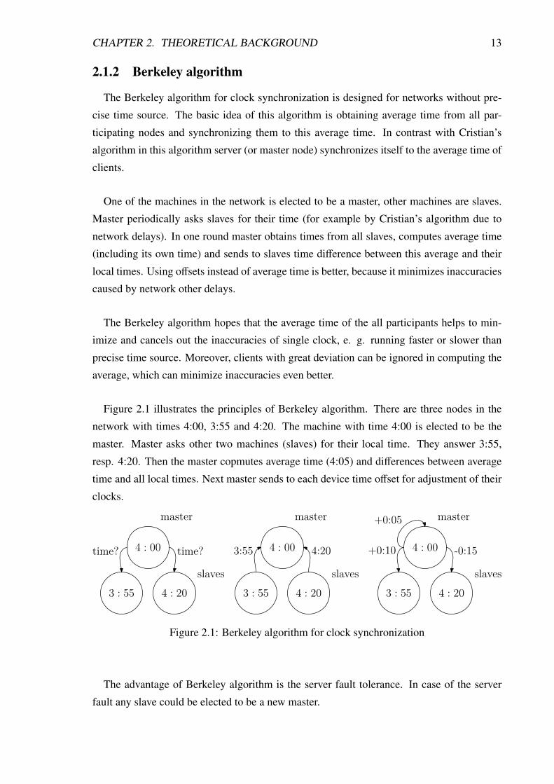
Figure 2.1 illustrates the principles of Berkeley algorithm. There are three nodes in the
network with times 4:00, 3:55 and 4:20. The machine with time 4:00 is elected to be the
master. Master asks other two machines (slaves) for their local time. They answer 3:55,
resp. 4:20. Then the master copmutes average time (4:05) and differences between average
time and all local times. Next master sends to each device time offset for adjustment of their
clocks.
4 : 00
3 : 55 4 : 20
master
slaves
time? time? 4 : 00
3 : 55 4 : 20
master
slaves
3:55 4:20 4 : 00
3 : 55 4 : 20
master
slaves
+0:05
+0:10 -0:15
Figure 2.1: Berkeley algorithm for clock synchronization
The advantage of Berkeley algorithm is the server fault tolerance. In case of the server
fault any slave could be elected to be a new master.
CHAPTER 2. THEORETICAL BACKGROUND 14
2.1.3 Network Time Protocol
The Network Time Protocol (version 3) is a standard (RFC 1305) for network synchro-
nization to Universal Coordinated Time despite network delays. Also provides protection
against interference and authenticates the reliability of data and their source.
This protocol is too complicated for my purposes, I included it to this list of clock syn-
chronization algorithms only for information and because it is the internet standard for clock
synchronization.
2.2 Sound analysis
Sound analysis is an important part of my application. I need to detect the presence of
certain frequencies in recorded sound, and I want to do this detection almost real-time.
Recorded data from microphone is nothing else than a sequence of bytes (or short inte-
gers or floats) periodically captured with some specific frequency called sample rate (usually
44100Hz, 22050 Hz, 11025Hz,. . . ). This is the way how from a continuous signal (ambient
sound) to make a discrete signal (digital data in machine).
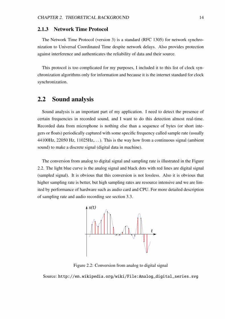
The conversion from analog to digital signal and sampling rate is illustrated in the Figure
2.2. The light blue curve is the analog signal and black dots with red lines are digital signal
(sampled signal). It is obvious that this conversion is not lossless. Also it is obvious that
higher sampling rate is better, but high sampling rates are resource intensive and we are lim-
ited by performance of hardware such as audio card and CPU. For more detailed description
of sampling rate and audio recording see section 3.3.
s(t)
t
Figure 2.2: Conversion from analog to digital signal
Source: http://en.wikipedia.org/wiki/File:Analog_digital_series.svg
CHAPTER 2. THEORETICAL BACKGROUND 15
Subsection about Fourier series is based on the lecture Základné matematické metódy
[BK11] and my handwritings from this lecture, subsections about Fourier transforms are
based on [Wei13d], [Wei13e], [Wei13a] and [Wei13b].
2.2.1 Fourier series
There are many periodical phenomenons in the real world. For example oscillations of
the springs, sound, heat engines,. . . These phenomena can be usually described with periodic
function f (t) with the least period T such that:
f (t + T ) = f (t) (2.1)
Sometimes it is advantageous to decompose complicated functions into series of elemen-
tary funcions. For example Taylor series is the decomposition of function into the power
series. We have two elementary periodical functions: sine and cosine. Now we can try
decompose every periodical function to series of sines and cosines:
f (t) = c0 +
∞∑i=1
(ci cos(ωit) + di sin(ωit)) (2.2)
For clarity we use sin(ωit) and cos(ωit), where ωi = 2πTi
is angular frequency and Ti is
period of this elementary periodic function. And we have fundamental frequency, resp.
fundamental angular frequency ω = 2πT correspinding to the least period T of function f .
Because function f is periodical and satisfy condition 2.1, we can write equation 2.2 in
other form:
c0 +
∞∑i=1
(ci cos(ωit) + di sin(ωit) = f (t) =
= f (t + T ) = c0 +
∞∑i=1
(ci cos (ωi(t + T )) + di sin (ωi(t + T )))
This equality holds if and only if ωiT = 2πni, where ni ∈ N. Dividing both sides of this
condition we have ωi = ωni. Now equation 2.2 has a form:
f (t) =a0
2+
∞∑n=1
(an cos(nωt) + bn sin(nωt)) (2.3)
CHAPTER 2. THEORETICAL BACKGROUND 16
Before we continue with determination of the coefficients an and bn, we solve some helpful
integrals.
∫ T
0cos(nωt)dt =
[sin(nωt)
nω
]T
0= 0 (2.4)∫ T
0sin(nωt)dt =
[−cos(nωt)
nω
]T
0= 0 (2.5)∫ T
0dt = [t]T
0 = T (2.6)∫ T
0cos(nωt) sin(mωt)dt =
∫ T
0
12
(sin
((n + m)ωt
)+ sin
((n − m)ωt
))= 0 (2.7)∫ T
0cos(nωt) cos(mωt)dt =
∫ T
0
12
(cos
((n + m)ωt
)+ cos
((n − m)ωt
))=
T2δn,m (2.8)∫ T
0sin(nωt) sin(mωt)dt =
∫ T
0
12
(cos
((n − m)ωt
)− cos
((n + m)ωt
))=
T2δn,m (2.9)
where n,m ∈ N and symbol δn,m =
0, if n , m
1, if n = mis Kronecker delta.
Now we can determine the coefficients an in equation 2.3. Multiplying both sides of 2.3
by cos(mωt), integrating from 0 to T and using integrals 2.4, 2.7 and 2.8 we obtain
∫ T
0f (t) cos(mωt)dt =
∫ T
0
a0
2cos(mωt)dt +
∞∑n=1
∫ T
0an cos(nωt) cos(mωt)dt +
+
∞∑n=1
∫ T
0bn sin(nωt) cos(mωt)dt = 0 +
∞∑n=1
anT2δn,m + 0 =
T2
am
am =2T
∫ T
0f (t) cos(mωt)dt (2.10)
Similarly we can determine the coeficients bn. Multiplying both sides of 2.3 by sin(mωt),
intergating from 0 to T and using integrals 2.5, 2.7 and 2.9 we obtain
∫ T
0f (t) sin(mωt)dt =
∫ T
0
a0
2sin(mωt)dt +
∞∑n=1
∫ T
0an cos(nωt) sin(mωt)dt +
+
∞∑n=1
∫ T
0bn sin(nωt) sin(mωt)dt = 0 + 0 +
∞∑n=1
bnT2δn,m =
T2
bm
bm =2T
∫ T
0f (t) sin(mωt)dt (2.11)
The coefficient a0 we can simply obtain by integrating of the equation2.3 from 0 to T and
using integral 2.6.
CHAPTER 2. THEORETICAL BACKGROUND 17
∫ T
0f (t)dt =
∫ T
0
a0
2dt +
∞∑n=1
∫ T
0an cos(nωt)dt +
∞∑n=1
∫ T
0bn sin(nωt)dt
=a0
2T + 0 + 0 =
a0
2T
a0 =2T
∫ T
0f (t)dt (2.12)
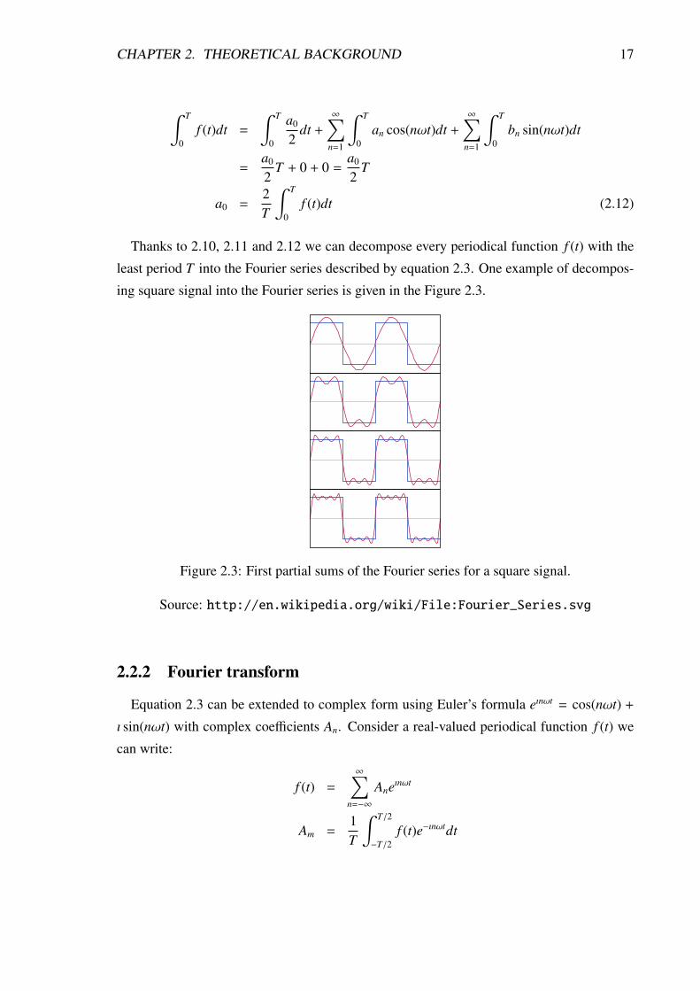
Thanks to 2.10, 2.11 and 2.12 we can decompose every periodical function f (t) with the
least period T into the Fourier series described by equation 2.3. One example of decompos-
ing square signal into the Fourier series is given in the Figure 2.3.
Figure 2.3: First partial sums of the Fourier series for a square signal.
Source: http://en.wikipedia.org/wiki/File:Fourier_Series.svg
2.2.2 Fourier transform
Equation 2.3 can be extended to complex form using Euler’s formula eınωt = cos(nωt) +
ı sin(nωt) with complex coefficients An. Consider a real-valued periodical function f (t) we
can write:
f (t) =
∞∑n=−∞
Aneınωt
Am =1T
∫ T/2
−T/2f (t)e−ınωtdt
CHAPTER 2. THEORETICAL BACKGROUND 18
Now generalize this series for T → ∞. Let the n/T = k, replace discrete An with continu-
ous function F(k). We obtain
f (t) =
∫ ∞
−∞
F(k)eı2πktdk
F(k) =
∫ ∞
−∞
f (t)e−ı2πktdt
These equations transform function of time f (t) to function of frequency F(k) and vice
versa. The new function F(k) is known also as a frequency spectrum of the function f (t).
2.2.3 Fast Fourier transform
The Fourier transform can be generalized to case of discrete function f (t). Let the f (t) be
f (tk), where tk are sampling points of function f (t) with difference ∆. Then we can write
f (tk) = f (k∆) as fk. With N sampling points, Discrete Fourier transform of sequence fk has
a form
Fn =
N−1∑k=0
fke−ı2πnk/N (2.13)
We want to compute all the Fn. If we compute them directly from equation 2.13, we need
O (N) steps for every Fn, so for all Fn we need O(N2
)steps. This is not very real-time
processing, so we can try to optimize this computation. Considering that N is a power of
two, we can rewrite 2.13 as
N−1∑k=0
fke−ı2πnk/N =
N/2−1∑k=0
f2ke−ı2πn(2k)/N +
N/2−1∑k=0
f2k+1e−ı2πn(2k+1)/N
=
N/2−1∑k=0
fevenke−ı2πn(k)/(N/2) + e−ı2πk/N
N/2−1∑k=0
foddke−ı2πnk/(N/2) (2.14)
Idea of equation 2.14 is that instead of compute Fourier transform of length N we compute
two Fourier transforms of length N/2 and merge them with O (N) steps. Due to Master
Theorem this yields in efficiency O(N log N
), which is much better than O
(N2
)and can be
computed almost real-time.
2.2.4 Implementation
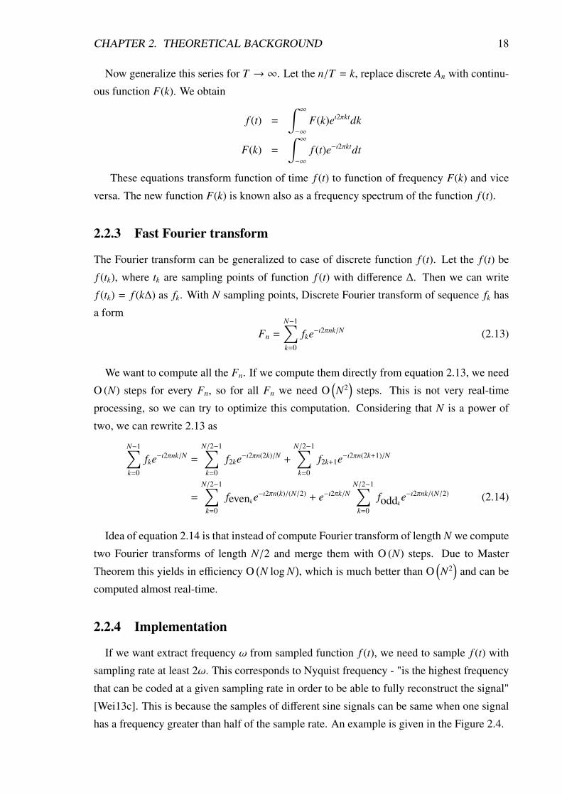
If we want extract frequency ω from sampled function f (t), we need to sample f (t) with
sampling rate at least 2ω. This corresponds to Nyquist frequency - "is the highest frequency
that can be coded at a given sampling rate in order to be able to fully reconstruct the signal"
[Wei13c]. This is because the samples of different sine signals can be same when one signal
has a frequency greater than half of the sample rate. An example is given in the Figure 2.4.
CHAPTER 2. THEORETICAL BACKGROUND 19
Figure 2.4: Identical sampling of the different sine signals
Source: http://en.wikipedia.org/wiki/File:CPT-sound-nyquist-thereom-1.
5percycle.svg
Because of the Nyquist frequency, in the implementation of the Fourier transform access
is provided only to first half of Fk. Moreover, these Fks are not exact frequencies, but the
frequency bands centered on given frequency. The number and width of frequency bands
depends on the size of sample and on the sampling rate. Let the size of sample be N and
sampling rate ω. Due to Nyquist frequency we can reconstruct N/2 frequencies below ω/2,
so the size of frequency band is ω/N.
According to these facts, I write a simple implementation of the Fourier transform. With
given sample in mSampleData with length mSampleSize function getBand(int index)
computes amplitude of complex coefficient Findex.
1 p u b l i c f l o a t getBand ( i n t i n d e x ) {
2 f l o a t N = mSampleSize ;
3 f l o a t a = 0 ;
4 f l o a t b = 0 ;
5 f o r ( i n t n = 0 ; n < N; n++) {
6 a += mSampleData [ n ] ∗ Floa tMa th . cos (2 ∗ Math . PI ∗ n ∗ i n d e x / N) ;
7 b += mSampleData [ n ] ∗ Floa tMa th . s i n (2 ∗ Math . PI ∗ n ∗ i n d e x / N) ;
8 }
9 f l o a t a m p l i t u d e = Floa tMa th . s q r t ( a ∗ a + b ∗ b ) ;
10 re turn a m p l i t u d e ;
11 }
Listing 2.1: Fourier transform
This is the Fourier transform with a complexity of O(N2
). Basic optimization can be done
by precomputing values of sin and cos, but even more optimization can be done by using
the Fast Fourier algorithm. I could implement it, but there is a good library with FFT called
Minim (http://code.compartmental.net/tools/minim/).
CHAPTER 2. THEORETICAL BACKGROUND 20
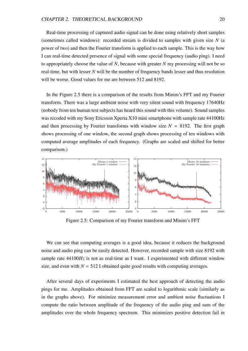
Real-time processing of captured audio signal can be done using relatively short samples
(sometimes called windows): recorded stream is divided to samples with given size N (a
power of two) and then the Fourier transform is applied to each sample. This is the way how
I can real-time detected presence of signal with some special frequency (audio ping). I need
to appropriately choose the value of N, because with greater N my processing will not be so
real-time, but with lesser N will be the number of frequency bands lesser and thus resolution
will be worse. Good values for me are between 512 and 8192.
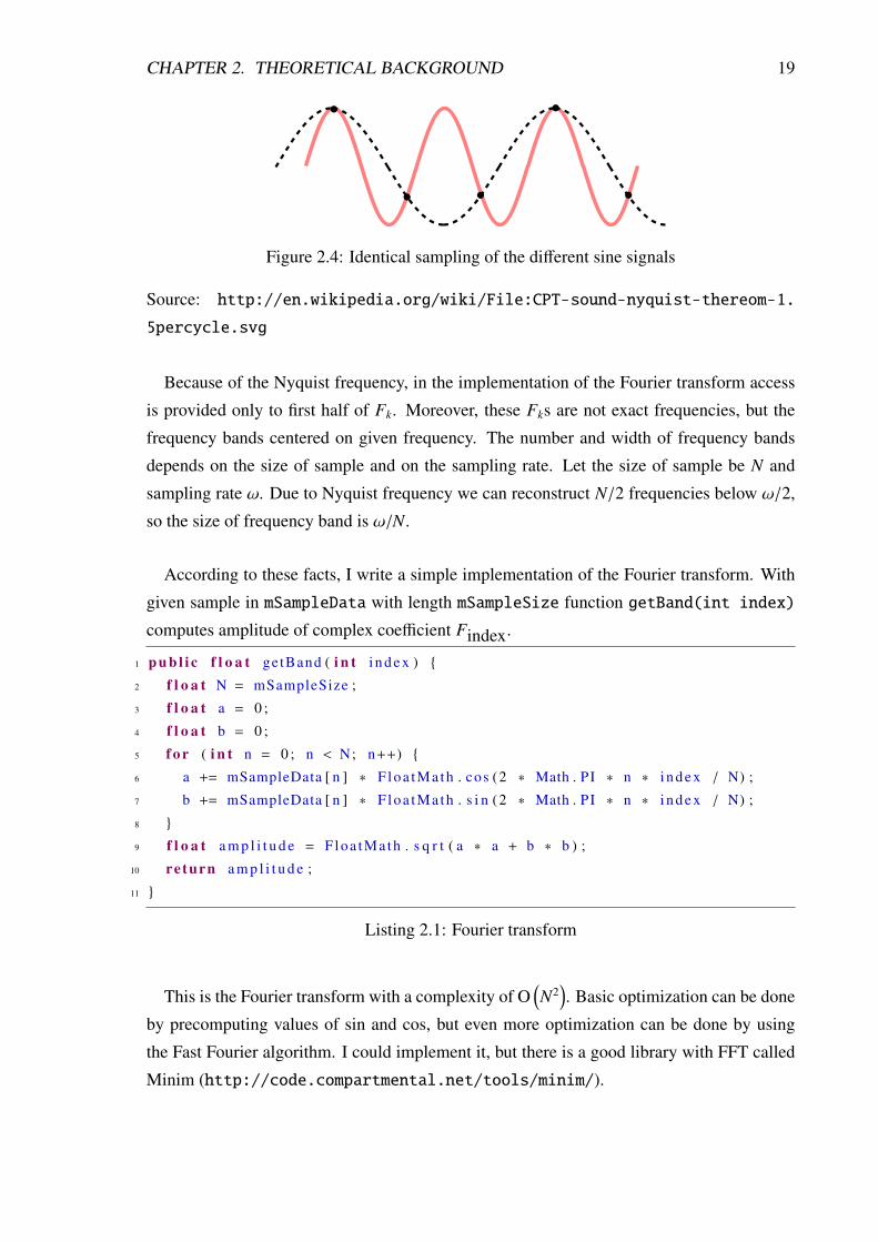
In the Figure 2.5 there is a comparison of the results from Minim’s FFT and my Fourier
transform. There was a large ambient noise with very silent sound with frequency 17640Hz
(nobody from ten human test subjects has heard this sound with this volume). Sound samples
was recoded with my Sony Ericsson Xperia X10 mini smartphone with sample rate 44100Hz
and then processing by Fourier transforms with window size N = 8192. The first graph
shows processing of one window, the second graph shows processing of ten windows with
computed average amplitudes of each frequency. (Graphs are scaled and shifted for better
comparison.)
-2
0
2
4
6
8
10
12
14
0 5000 10000 15000 20000 25000
Minim 1 windowMy Fourier 1 window
0
2
4
6
8
10
12
14
0 5000 10000 15000 20000 25000
Minim 10 windowsMy Fourier 10 windows
Figure 2.5: Comparison of my Fourier transform and Minim’s FFT
We can see that computing averages is a good idea, because it reduces the background
noise and audio ping can be easily detected. However, recorded sample with size 8192 with
sample rate 44100Hz is not as real-time as I want. I experimented with different window
size, and even with N = 512 I obtained quite good results with computing averages.
After several days of experiments I estimated the best approach of detecting the audio
pings for me. Amplitudes obtained from FFT are scaled to logarithmic scale (similarly as
in the graphs above). For minimize measurement error and ambient noise fluctuations I
compute the ratio between amplitude of the frequency of the audio ping and sum of the
amplitudes over the whole frequency spectrum. This minimizes positive detection fail in
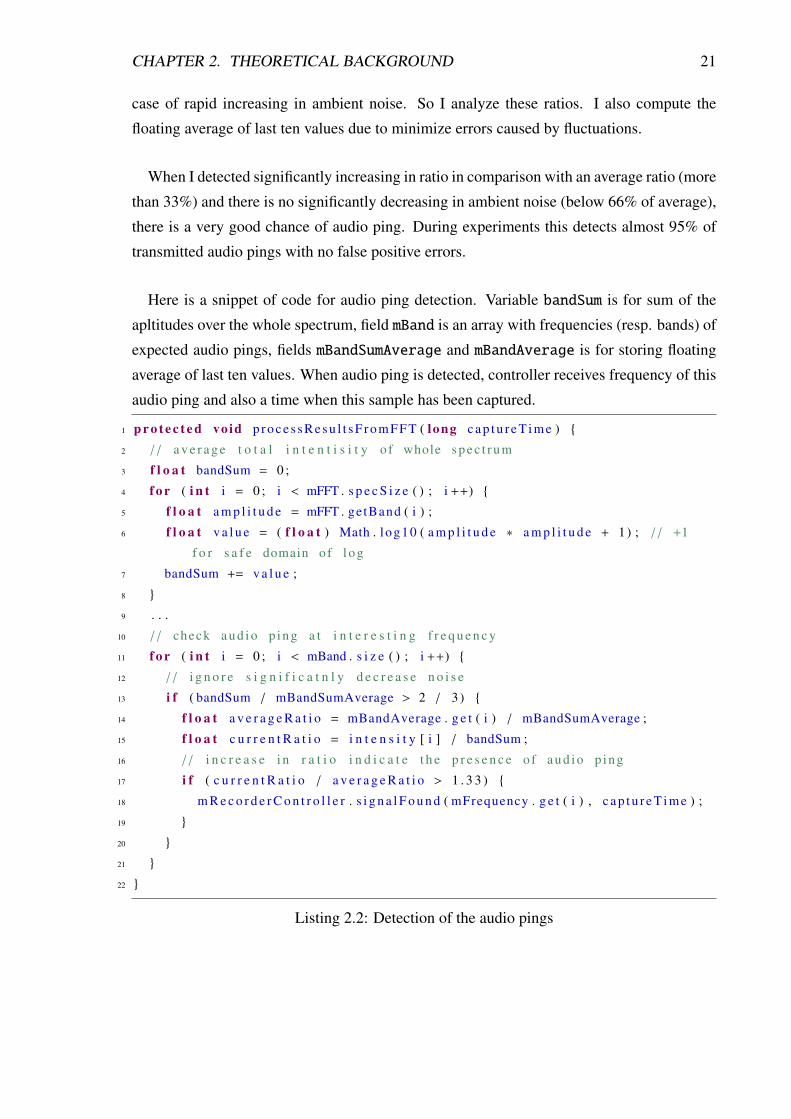
CHAPTER 2. THEORETICAL BACKGROUND 21
case of rapid increasing in ambient noise. So I analyze these ratios. I also compute the
floating average of last ten values due to minimize errors caused by fluctuations.
When I detected significantly increasing in ratio in comparison with an average ratio (more
than 33%) and there is no significantly decreasing in ambient noise (below 66% of average),
there is a very good chance of audio ping. During experiments this detects almost 95% of
transmitted audio pings with no false positive errors.
Here is a snippet of code for audio ping detection. Variable bandSum is for sum of the
apltitudes over the whole spectrum, field mBand is an array with frequencies (resp. bands) of
expected audio pings, fields mBandSumAverage and mBandAverage is for storing floating
average of last ten values. When audio ping is detected, controller receives frequency of this
audio ping and also a time when this sample has been captured.
1 p r o t e c t e d void p ro c e s s R e su l t sF r om F F T ( long c a p t u r e T i m e ) {
2 / / a v e r a g e t o t a l i n t e n t i s i t y o f whole s p e c t r u m
3 f l o a t bandSum = 0 ;
4 f o r ( i n t i = 0 ; i < mFFT . s p e c S i z e ( ) ; i ++) {
5 f l o a t a m p l i t u d e = mFFT . getBand ( i ) ;
6 f l o a t v a l u e = ( f l o a t ) Math . log10 ( a m p l i t u d e ∗ a m p l i t u d e + 1) ; / / +1
f o r s a f e domain o f l o g
7 bandSum += v a l u e ;
8 }
9 . . .
10 / / check a u d i o p ing a t i n t e r e s t i n g f r e q u e n c y
11 f o r ( i n t i = 0 ; i < mBand . s i z e ( ) ; i ++) {
12 / / i g n o r e s i g n i f i c a t n l y d e c r e a s e n o i s e
13 i f ( bandSum / mBandSumAverage > 2 / 3) {
14 f l o a t a v e r a g e R a t i o = mBandAverage . g e t ( i ) / mBandSumAverage ;
15 f l o a t c u r r e n t R a t i o = i n t e n s i t y [ i ] / bandSum ;
16 / / i n c r e a s e i n r a t i o i n d i c a t e t h e p r e s e n c e o f a u d i o p ing
17 i f ( c u r r e n t R a t i o / a v e r a g e R a t i o > 1 . 3 3 ) {
18 m R e c o r d e r C o n t r o l l e r . s i g n a l F o u n d ( mFrequency . g e t ( i ) , c a p t u r e T i m e ) ;
19 }
20 }
21 }
22 }
Listing 2.2: Detection of the audio pings
Chapter 3
Android application
3.1 Architecture
This section is based mainly on [Goo13f], [Kon12] and my own experiences.
The elementary part of Android application is a unit called Activity. We can simply imag-
ine that Activity is like a controller or presenter from MVC/P design patterns. However, this
is not entirely true. Although the task of the Activity is obtaining data from lower levels of
application (models) and displaying them to the user, the Android application does not have
a classical view from MVC/P. Activity is something between the view and the controller/p-
resenter and we could say that Activity is the presentation layer of the application.
Another elementary unit of Android applications is the View. If the Activity is something
like controller/presenter from web MVC/P, then View is something like HTML. The View
can be created programmatically or can be written in XML file. Activity creates all its view
and then uses them for displaying and obtaining data.
With Android 3.0 Honeycomb Google has introduced Fragments. Fragments can be used
as a part of application layout for better modularization. It is especially helpful for designing
layout suitable both for tablets and smartphones. Fragments can encapsulate some logi-
cal unit, such as Views with methods related to them. Activity can use many fragments to
achieve responsive design and better user interface. Fragments bring a new layer between
Views and Activities. But I require that my application must be compatible with older ver-
sions of Android (especially Android 2.1 because my Xperia X10 mini has this version of
operating system). Fortunately, Google published Support Library which brings some of
the new API for the older platform versions. In case of fragments, this library comes with
support from API level 4 (Android 1.6). This is a good message for me and my requirements.
22
CHAPTER 3. ANDROID APPLICATION 23
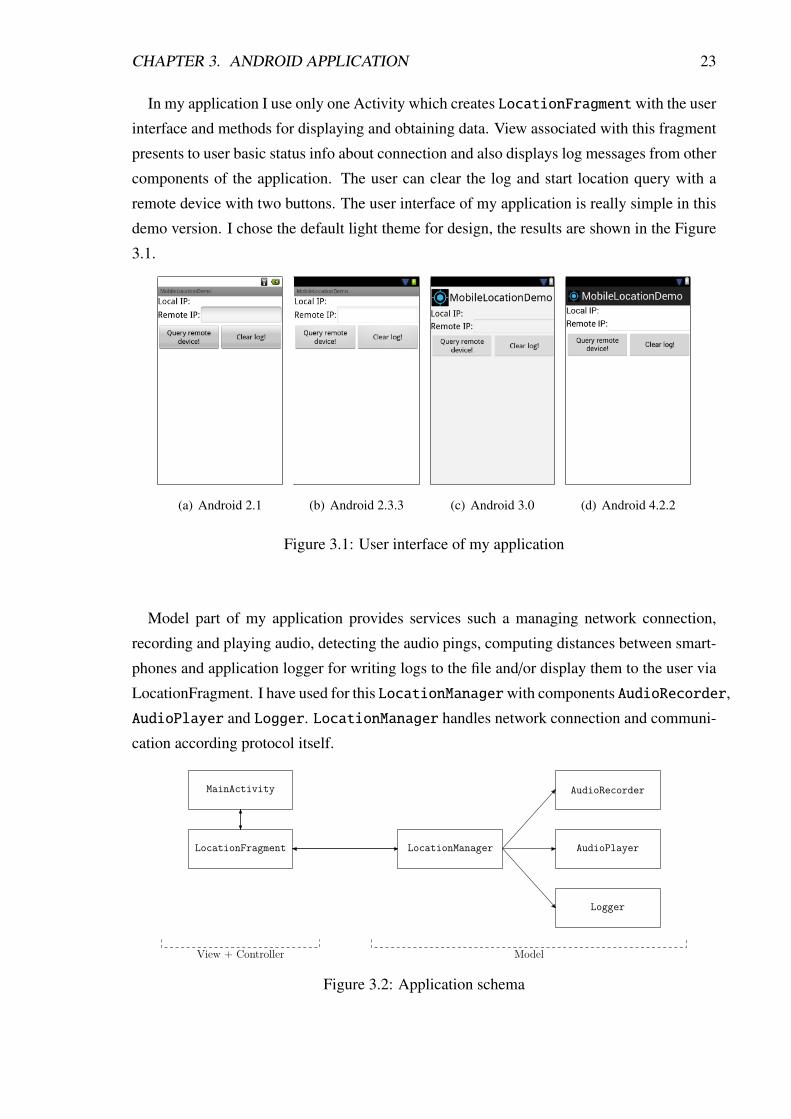
In my application I use only one Activity which creates LocationFragmentwith the user
interface and methods for displaying and obtaining data. View associated with this fragment
presents to user basic status info about connection and also displays log messages from other
components of the application. The user can clear the log and start location query with a
remote device with two buttons. The user interface of my application is really simple in this
demo version. I chose the default light theme for design, the results are shown in the Figure
3.1.
(a) Android 2.1 (b) Android 2.3.3 (c) Android 3.0 (d) Android 4.2.2
Figure 3.1: User interface of my application
Model part of my application provides services such a managing network connection,
recording and playing audio, detecting the audio pings, computing distances between smart-
phones and application logger for writing logs to the file and/or display them to the user via
LocationFragment. I have used for this LocationManagerwith components AudioRecorder,
AudioPlayer and Logger. LocationManager handles network connection and communi-
cation according protocol itself.
MainActivity
LocationFragment LocationManager
AudioRecorder
AudioPlayer
Logger
View + Controller Model
Figure 3.2: Application schema
CHAPTER 3. ANDROID APPLICATION 24
3.2 Bluetooth and WiFi
Important part of my application is the communication between smartphones for short
distances. I do not need Internet and moreover, the Internet is not suitable for my purposes,
because not everyone user has an Internet connection (Edge or 3G or LTE) in his smartphone.
The prizes of roaming in abroad are too high and using the Internet with other than own
operator is not cheap.
My first choice is the Bluetooth. Bluetooth has been designed for exchanging data over
short distances, so it could be appropriate for me. But after more detailed examination of this
technology, I discovered many disadvantages for me. Here I briefly describe these problems.
Bluetooth networks are called piconets with master-slave structure. In each piconet there
is one master and up to 7 slaves. So in one piconet can be up to 8 devices connected through
master. This is not very usable for communication between each pair of nodes. In the
future, I like to use my application for localization of smartphones in networks with many
devices (scenarios from Introduction). So I will need Bluetooth network with more than 8
nodes. Bluetooth as a large-scale ad hoc networking technology is discussed in [VGSR05].
Available solutions are too complicated for my purposes. Moreover, with many piconets
in the same location there will be increasing in probability of mutual interference, this is
discussed in [How03].
Another problem is pairing devices. When connection is made for the first time, pairing
request is automatically presented to the user. And without user’s confirmation of pairing
there is no official way for creating Bluetooth communication channel between two devices
with older Android than v2.3.3 (API 10).
In API 10 there has been added a support for insecure RFCOMM BluetoothSocket with
BluetoothDevice’s method createInsecureRfcommSocketToServiceRecord(uuid)
[Goo13c]. But as I mentioned before, I want to support devices with API 7 and latter.
Because these big disadvantages I decided to forget about Bluetooth. So I have to make
connection via WiFi. I hope that at least one device in test scenario has a capability for
creating WiFi Hotspot (support has been added in Android 2.2) or there is an available WiFi
network. Note: I do not use WiFi Direct due to lack of the support on Android older than
v4.0.
In my application the LocationManager is responsible for managing communication
between devices. First of all, I check if the device is connected to a WiFi network. If yes, I
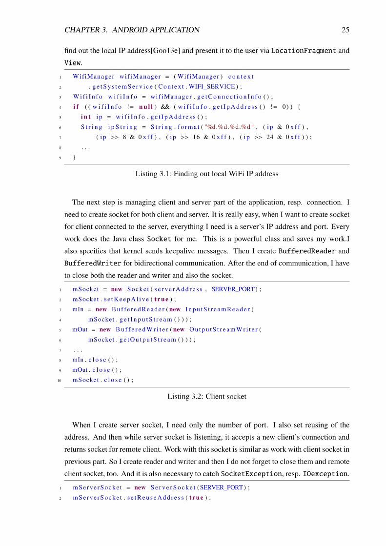
CHAPTER 3. ANDROID APPLICATION 25
find out the local IP address[Goo13e] and present it to the user via LocationFragment and
View.
1 WifiManager wi f iManager = ( WifiManager ) c o n t e x t
2 . g e t S y s t e m S e r v i c e ( C o n t e x t . WIFI_SERVICE ) ;
3 W i f i I n f o w i f i I n f o = wif iManage r . g e t C o n n e c t i o n I n f o ( ) ;
4 i f ( ( w i f i I n f o != n u l l ) && ( w i f i I n f o . g e t I p A d d r e s s ( ) != 0) ) {
5 i n t i p = w i f i I n f o . g e t I p A d d r e s s ( ) ;
6 S t r i n g i p S t r i n g = S t r i n g . f o r m a t ( "%d.%d.%d.%d " , ( i p & 0 x f f ) ,
7 ( i p >> 8 & 0 x f f ) , ( i p >> 16 & 0 x f f ) , ( i p >> 24 & 0 x f f ) ) ;
8 . . .
9 }
Listing 3.1: Finding out local WiFi IP address
The next step is managing client and server part of the application, resp. connection. I
need to create socket for both client and server. It is really easy, when I want to create socket
for client connected to the server, everything I need is a server’s IP address and port. Every
work does the Java class Socket for me. This is a powerful class and saves my work.I
also specifies that kernel sends keepalive messages. Then I create BufferedReader and
BufferedWriter for bidirectional communication. After the end of communication, I have
to close both the reader and writer and also the socket.
1 mSocket = new So ck e t ( s e r v e r A d d r e s s , SERVER_PORT) ;
2 mSocket . s e t K e e p A l i v e ( t rue ) ;
3 mIn = new B u f f e r e d R e a d e r ( new I n p u t S t r e a m R e a d e r (
4 mSocket . g e t I n p u t S t r e a m ( ) ) ) ;
5 mOut = new B u f f e r e d W r i t e r ( new O u t p u t S t r e a m W r i t e r (
6 mSocket . g e t O u t p u t S t r e a m ( ) ) ) ;
7 . . .
8 mIn . c l o s e ( ) ;
9 mOut . c l o s e ( ) ;
10 mSocket . c l o s e ( ) ;
Listing 3.2: Client socket
When I create server socket, I need only the number of port. I also set reusing of the
address. And then while server socket is listening, it accepts a new client’s connection and
returns socket for remote client. Work with this socket is similar as work with client socket in
previous part. So I create reader and writer and then I do not forget to close them and remote
client socket, too. And it is also necessary to catch SocketException, resp. IOexception.
1 mServe rSocke t = new S e r v e r S o c k e t (SERVER_PORT) ;
2 mServe rSocke t . s e t R e u s e A d d r e s s ( t rue ) ;
CHAPTER 3. ANDROID APPLICATION 26
3 whi le ( l i s t e n i n g ) {
4 mRemoteCl ien tSocke t = mServe rSocke t . a c c e p t ( ) ;
5 mRemoteCl ien tSocke t . s e t K e e p A l i v e ( t rue ) ;
6 mIn = new B u f f e r e d R e a d e r ( new I n p u t S t r e a m R e a d e r (
7 mRemoteCl ien tSocke t . g e t I n p u t S t r e a m ( ) ) ) ;
8 mOut = new B u f f e r e d W r i t e r ( new O u t p u t S t r e a m W r i t e r (
9 mRemoteCl ien tSocke t . g e t O u t p u t S t r e a m ( ) ) ) ;
10 . . .
11 mIn . c l o s e ( ) ;
12 mOut . c l o s e ( ) ;
13 mRemoteCl ien tSocke t . c l o s e ( ) ;
14 }
15 . . .
16 mServe rSocke t . c l o s e ( ) ;
Listing 3.3: Server socket
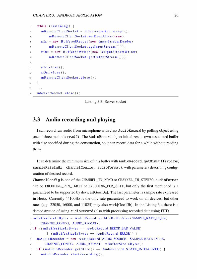
3.3 Audio recording and playing
I can record raw audio from microphone with class AudioRecord by polling object using
one of three methods read(). The AudioRecord object initializes its own associated buffer
with size specified during the construction, so it can record data for a while without reading
them.
I can determine the minimum size of this buffer with AudioRecord.getMinBufferSize(
sampleRateInHz, channelConfig, audioFormat), with parameters describing config-
uration of desired record.
ChannelConfig is one of the CHANNEL_IN_MONO or CHANNEL_IN_STEREO, audioFormat
can be ENCODING_PCM_16BIT or ENCODING_PCM_8BIT, but only the first mentioned is a
guaranteed to be supported by devices[Goo13a]. The last parameter is sample rate expressed
in Hertz. Currently 44100Hz is the only rate guaranteed to work on all devices, but other
rates (e.g. 22050, 16000, and 11025) may also work[Goo13b]. In the Listing 3.4 there is a
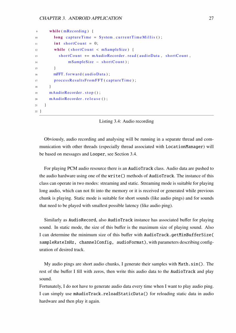
demonstration of using AudioRecord (also with processing recorded data using FFT).
1 m B u f f e r S i z e I n B y t e s = AudioRecord . g e t M i n B u f f e r S i z e (SAMPLE_RATE_IN_HZ ,
2 CHANNEL_CONFIG, AUDIO_FORMAT) ;
3 i f ( ( m B u f f e r S i z e I n B y t e s == AudioRecord .ERROR_BAD_VALUE)
4 | | ( m B u f f e r S i z e I n B y t e s == AudioRecord .ERROR) ) {
5 mAudioRecorder = new AudioRecord (AUDIO_SOURCE, SAMPLE_RATE_IN_HZ ,
6 CHANNEL_CONFIG, AUDIO_FORMAT, m B u f f e r S i z e I n B y t e s ) ;
7 i f ( mAudioRecorder . g e t S t a t e ( ) == AudioRecord . STATE_INITIALIZED ) {
8 mAudioRecorder . s t a r t R e c o r d i n g ( ) ;
CHAPTER 3. ANDROID APPLICATION 27
9 whi le ( mRecording ) {
10 long c a p t u r e T i m e = System . c u r r e n t T i m e M i l l i s ( ) ;
11 i n t s h o r t C o u n t = 0 ;
12 whi le ( s h o r t C o u n t < mSampleSize ) {
13 s h o r t C o u n t += mAudioRecorder . r e a d ( aud ioData , s h o r t C o u n t ,
14 mSampleSize − s h o r t C o u n t ) ;
15 }
16 mFFT . f o r w a r d ( a u d i o D a t a ) ;
17 p ro c e s s R e su l t sF r om F F T ( c a p t u r e T i m e ) ;
18 }
19 mAudioRecorder . s t o p ( ) ;
20 mAudioRecorder . r e l e a s e ( ) ;
21 }
22 }
Listing 3.4: Audio recording
Obviously, audio recording and analysing will be running in a separate thread and com-
munication with other threads (especially thread associated with LocationManager) will
be based on messages and Looper, see Section 3.4.
For playing PCM audio resource there is an AudioTrack class. Audio data are pushed to
the audio hardware using one of the write() methods of AudioTrack. The instance of this
class can operate in two modes: streaming and static. Streaming mode is suitable for playing
long audio, which can not fit into the memory or it is received or generated while previous
chunk is playing. Static mode is suitable for short sounds (like audio pings) and for sounds
that need to be played with smallest possible latency (like audio ping).
Similarly as AudioRecord, also AudioTrack instance has associated buffer for playing
sound. In static mode, the size of this buffer is the maximum size of playing sound. Also
I can determine the minimum size of this buffer with AudioTrack.getMinBufferSize(
sampleRateInHz, channelConfig, audioFormat), with parameters describing config-
uration of desired track.
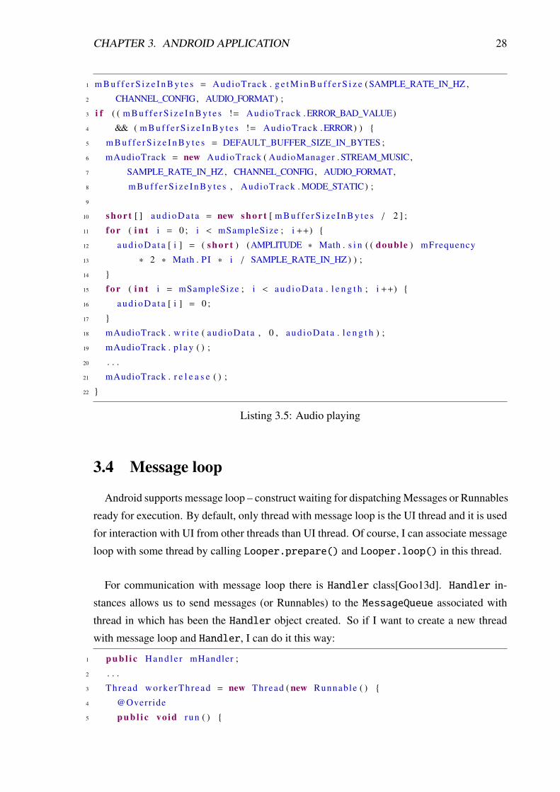
My audio pings are short audio chunks, I generate their samples with Math.sin(). The
rest of the buffer I fill with zeros, then write this audio data to the AudioTrack and play
sound.
Fortunately, I do not have to generate audio data every time when I want to play audio ping.
I can simply use mAudioTrack.reloadStaticData() for reloading static data in audio
hardware and then play it again.
CHAPTER 3. ANDROID APPLICATION 28
1 m B u f f e r S i z e I n B y t e s = AudioTrack . g e t M i n B u f f e r S i z e (SAMPLE_RATE_IN_HZ ,
2 CHANNEL_CONFIG, AUDIO_FORMAT) ;
3 i f ( ( m B u f f e r S i z e I n B y t e s != AudioTrack .ERROR_BAD_VALUE)
4 && ( m B u f f e r S i z e I n B y t e s != AudioTrack .ERROR) ) {
5 m B u f f e r S i z e I n B y t e s = DEFAULT_BUFFER_SIZE_IN_BYTES ;
6 mAudioTrack = new AudioTrack ( AudioManager . STREAM_MUSIC,
7 SAMPLE_RATE_IN_HZ , CHANNEL_CONFIG, AUDIO_FORMAT,
8 m B u f f e r S i z e I n B y t e s , AudioTrack . MODE_STATIC) ;
9
10 s h o r t [ ] a u d i o D a t a = new s h o r t [ m B u f f e r S i z e I n B y t e s / 2 ] ;
11 f o r ( i n t i = 0 ; i < mSampleSize ; i ++) {
12 a u d i o D a t a [ i ] = ( s h o r t ) (AMPLITUDE ∗ Math . s i n ( ( double ) mFrequency
13 ∗ 2 ∗ Math . PI ∗ i / SAMPLE_RATE_IN_HZ) ) ;
14 }
15 f o r ( i n t i = mSampleSize ; i < a u d i o D a t a . l e n g t h ; i ++) {
16 a u d i o D a t a [ i ] = 0 ;
17 }
18 mAudioTrack . w r i t e ( aud ioData , 0 , a u d i o D a t a . l e n g t h ) ;
19 mAudioTrack . p l a y ( ) ;
20 . . .
21 mAudioTrack . r e l e a s e ( ) ;
22 }
Listing 3.5: Audio playing
3.4 Message loop
Android supports message loop – construct waiting for dispatching Messages or Runnables
ready for execution. By default, only thread with message loop is the UI thread and it is used
for interaction with UI from other threads than UI thread. Of course, I can associate message
loop with some thread by calling Looper.prepare() and Looper.loop() in this thread.
For communication with message loop there is Handler class[Goo13d]. Handler in-
stances allows us to send messages (or Runnables) to the MessageQueue associated with
thread in which has been the Handler object created. So if I want to create a new thread
with message loop and Handler, I can do it this way:
1 p u b l i c Hand le r mHandler ;
2 . . .
3 Thread workerThread = new Thread ( new Runnable ( ) {
4 @Override
5 p u b l i c vo id run ( ) {
CHAPTER 3. ANDROID APPLICATION 29
6 Looper . p r e p a r e ( ) ;
7 mHandler = new Hand le r ( ) ;
8 Looper . l oop ( ) ;
9 }
10 } ) ;
11 workerThread . s t a r t ( ) ;
Listing 3.6: Thread with message loop
Interaction with workerThread can be done using one of post*() methods, such as
post(runnable), postAtTime(runnable, uptimeMillis) or postDelayed(runnable,
delayMillis).
1 mHandler . p o s t ( new Runnable ( ) {
2 @Override
3 p u b l i c vo id run ( ) {
4 . . .
5 }
6 } ) ;
Listing 3.7: Interaction with Handler
Message loop allows me to design control logic of distance measurement including send-
ing audio pings, processing detected audio pings, network communication between smart-
phones and evaluating the results.
3.5 Communication protocol of measurement
In my application two devices will communicate over the WiFi and will play and listen
for audio pings during measurement. All steps of this measurement must have exact order,
so I introduce the first version of communication protocol of measurement between these
smartphones.
1. the client makes a connection to the server
2. the client sends message M1 to the server and estimate local time ts0
3. the server sends timestamp T to the client
4. the client received server’s timestamp at local time t1, computes server’s current time
as T + (t1 − t0)/2 and offset ∆t to the local time (Cristian’s algorithm)
5. (optional) repeat steps 2 – 4 for better accuracy of time synchronization
6. the server sets time limit for audioping detection and sends message M2 to the client
7. the client plays audio ping and estimate time tc
CHAPTER 3. ANDROID APPLICATION 30
8. the server detects audio ping or timelimit, estimates time ts and sends ts to the client or
informs client about the time limit exceeding
9. if detection of audio ping was correct, the client computes travelling time of audio ping
as tt = ts − (tc + ∆t) and sends tt to the server; starts new measurement otherwise
The individual steps of this protocol can be simply programmed as the Runnable objects
and processed in the given order with the message loop associated with LocationManager’s
thread. Time limit for audio ping detection can be set with mHandler.postDelayed(r,
timelimit) in step 6. When detection of audio ping fails, then after timelimit exceeds,
Runnable r in the message loop will be processed. When detection of audio ping is correct,
then runnable for processing audio ping signal found action will be executed before runnable
for time limit and thus runnable for time limit can be ignored (first runnable sets some flag
for correct detection).
3.6 Experiments and problems
First of all, I programmed classes MainActivity, LocationFragment and AudioRecord
for testing purposes. Audio pings were generated in Audacity and played from the notebook.
In the beginning, audio ping recognition was very simple and dummy, I checked only am-
plitudes of audio ping’s frequency and if this amplitude was greater than some threshold, I
figured out this as the audio ping. This approach does not work as good as I want on my
Xperia X10 mini, because some audio pings were not recognized and some fluctuations in
ambient noise were recognized as audio pings.
I experimented with different durations of audio pings and different sizes of FFT’s window,
but there was detection fails with short durations and small sizes and performance and real-
time problems with long durations and large sizes. After many experiments and consultation
with my supervisor I figure out new approach described in Subsection 2.2.4. Described
method and implementation works great, recognition’s percentage of audio pings is above
95% in the test environment and detection of ambient noise as the audio pings is almost zero.
The next step was the implementation of AudioPlayer. For obvious reasons AudioTrack
is used in the static mode with 44100Hz sample rate, 16bit PCM encoding and mono channel
configuration. At first it seemed to be all OK with playing audio pings, but after a while I
noticed problems with repeated playing AudioTrack’s buffer. The correct way of replaying
is to call AudioTrack.stop() before AudioTrack.reloadStaticData(). With this fix
replaying of audio pings works perfect.
CHAPTER 3. ANDROID APPLICATION 31
With working classes AudioRecord and AudioPlayer I tried out to estimate the latency
of playing sound in static mode of AudioTrack. I was really disappointed, because the
latencies was approximately 100 milliseconds. This is indeed a too great value for my pur-
pose. With a 100 ms inaccuracy in audio playing measurements of travelling times will be
also too inacurate regardless of the time synchronization. I have to make small changes in
my approach and communication protocol.
3.7 Enhanced protocol and results
Latencies (and especially inaccuracies) in audio playing is good reason for a change in
my approach. But it is not so bad, smartphone can detect its own audio ping and estimate
time, when audio ping was really played. So I can switch to model more similar to the active
sonar. First smartphone sends audio ping to the second smartphone. When second device
receives this audio ping, plays own audio ping (at another frequency). Both devices can
detect these two audio pings and estimate times, when these pings were played or received.
In this measurement synchronizing clock are not necessary, because local time differences
are important, not exact local times. So I introduce enhanced protocol.
1. the client makes a connection
2. both the server and the client starts recorder
3. the client sends message M1 to the server, the server sends the same message to the
client1
4. both the client and the server sets time limit for audioping detection
5. the client waits d ms2 and plays audioping at frequency f1
6. both the server and the client detects audiopings or time limits, estimates time ts1 , tc1 ,
sets time limit for second audio ping detection
7. the server plays audioping at frequency f2
8. both the server and the client detects audiopings or time limits, estimates time ts2 , tc2
9. N times repeat steps 3 – 8
10. both the client and the server stops recorder
11. the server sends all ts2 − ts1 to the client over the WiFi
12. the client sends all tc2 − tc1 to the server over the WiFi
13. both the server and the client validates values due to time limits and calculates average
value of(tc2 − tc1
)−
(ts2 − ts1
)and standard deviation s
14. the server restarts listening and waiting for new clients
1reading from Reader is blocking operation, so it can be used as such a synchronization of the measurement
beginning2for a small pause between measurements
CHAPTER 3. ANDROID APPLICATION 32
In enhanced protocol, devices repeat measurements and computes averages for minimize
inaccuracies. Standard deviation is some indicator of the accuracy of this series of measure-
ments. Inaccuracy in the single measurement is really large, because all the times ts and tc
are approximately 150 – 350 ms, but their difference should be approximately 5 – 100 ms.
So differences are approximately the same as inacuraccies in single measurements. In single
measurements, it is often possible that estimated travelling time is less than zero, which is
not very good.
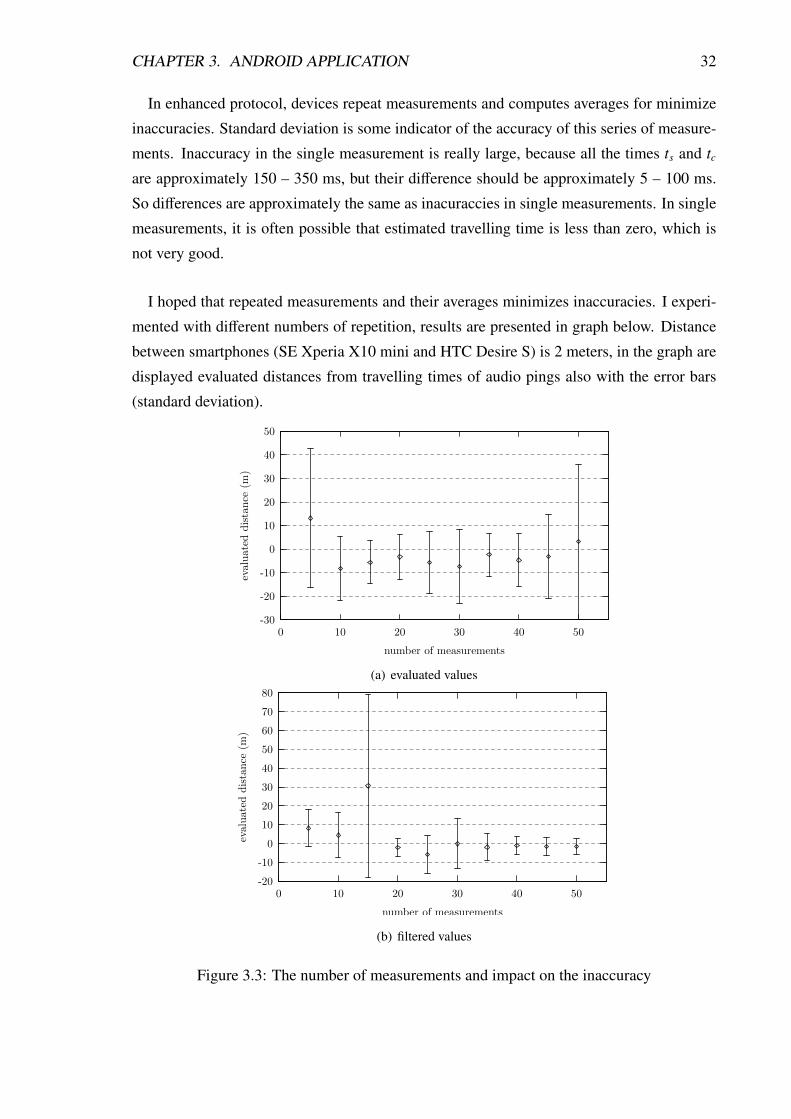
I hoped that repeated measurements and their averages minimizes inaccuracies. I experi-
mented with different numbers of repetition, results are presented in graph below. Distance
between smartphones (SE Xperia X10 mini and HTC Desire S) is 2 meters, in the graph are
displayed evaluated distances from travelling times of audio pings also with the error bars
(standard deviation).
-30
-20
-10
0
10
20
30
40
50
0 10 20 30 40 50
evaluateddistance
(m)
number of measurements
(a) evaluated values
-20
-10
0
10
20
30
40
50
60
70
80
0 10 20 30 40 50
evaluated
distance
(m)
number of measurements
(b) filtered values
Figure 3.3: The number of measurements and impact on the inaccuracy
CHAPTER 3. ANDROID APPLICATION 33
With increasing in the number of experiments, first there is expected decreasing in the
inaccuracy, but then inaccuracy raises again. This is because with more measurements there
is greater chance of occurrence of the measurement error. So I filtered out values with varia-
tion from average is greater than 3s. Results are shown in the Figure 3.3(b). As I expected,
this filtration brings better results especially for a greater number of measurements. But 50
measurements are too slow for practical application. Fortunately, also 20 – 25 measurements
have usually not so large inaccuracy.
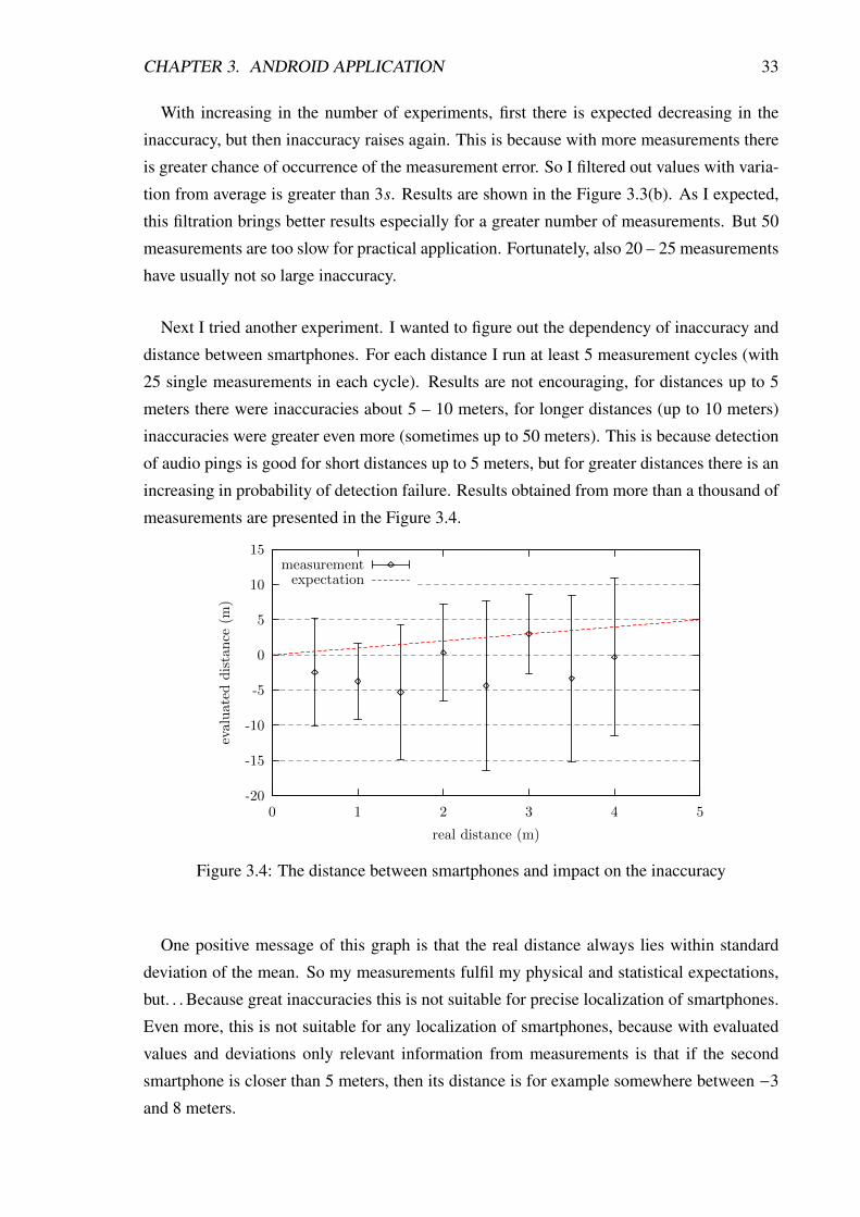
Next I tried another experiment. I wanted to figure out the dependency of inaccuracy and
distance between smartphones. For each distance I run at least 5 measurement cycles (with
25 single measurements in each cycle). Results are not encouraging, for distances up to 5
meters there were inaccuracies about 5 – 10 meters, for longer distances (up to 10 meters)
inaccuracies were greater even more (sometimes up to 50 meters). This is because detection
of audio pings is good for short distances up to 5 meters, but for greater distances there is an
increasing in probability of detection failure. Results obtained from more than a thousand of
measurements are presented in the Figure 3.4.
-20
-15
-10
-5
0
5
10
15
0 1 2 3 4 5
evaluateddistance
(m)
real distance (m)
measurementexpectation
Figure 3.4: The distance between smartphones and impact on the inaccuracy
One positive message of this graph is that the real distance always lies within standard
deviation of the mean. So my measurements fulfil my physical and statistical expectations,
but. . . Because great inaccuracies this is not suitable for precise localization of smartphones.
Even more, this is not suitable for any localization of smartphones, because with evaluated
values and deviations only relevant information from measurements is that if the second
smartphone is closer than 5 meters, then its distance is for example somewhere between −3
and 8 meters.
CHAPTER 3. ANDROID APPLICATION 34
Major contribution to inaccuracies is caused by thread scheduler, Dalvik Virtual Machine
and operating system itself. Android is not a real-time operating system, and at critical
moments there is not guaranteed something like maximum latency. Moreover, this latency is
compouded by Dalvik VM and Java itself.
My application estimated times in AudioRecorder’s thread, but when audio hardware
is recording sound and this thread is paused, estimation of the time will be delayed until
AudioRecorder’s thread will resume. And this delay depends on many parameters, such as
the system load and strategy of scheduler. And during long measurements, this parameters
can significantly affect latency in the estimation of the time when audio chunk has been
captured.
However, the audio ping detection works almost with all the tested smartphones: Sony
Ericsson Xperia X10 mini, Samsung Galaxy 5, Samsung Galaxy Mini, Samsung Galaxy S2
and HTC Desire S. This detection does not work only with Google Nexus One, because this
smartphone has an extra microphone for filtering audio input and it filters high frequencies
from recorded sound.
The audio ping detection can be useful in other applications. For example it can be a
medium for short-distance communication or for sending short notification between smart-
phones. Of course, the transfer rate will be much lesser than transfer rates of WiFi, Bluetooth
or NFC, but there is advantage in very simple broadcastig. Moreover, with parallel transmit-
ted audio pings at distinct frequencies will be the transfer rate greater. This can be useful for
example in supermarkets. There can be one transmitter in each department of supermarket
and it can inform customers in this department about current product’s discounts.
Another application can be an emulation of serial port for smartphones. Many devices
still use RS232 interface for communication, but these devices can not be simply connected
to the smartphones or tablets. With audio analysis, it RS232 interface can be emulated with
Jack port of smartphones. Or we can use audio analysis for recognition Morse code and
translation Morse code into Latin alphabet chars.
Conclusion
In this bachelor thesis I deal with possible approaches for short distance localization of
mobile devices, which is not based on GPS and has minimal prerequisites. Due to prereq-
uisites, most of available localization methods are not suitable, because they require some
external resources, such as Internet connection, access to database of the mobile cells or
WiFi access points (or GPS satellites).
After research of available technologies and features of smartphones, I decided to use
sound. There are two possible ways how to use sound for measuring distances between
smartphones, first is based on sound strength, second on sound speed. At the first touch the
sound intensity looks like a solution for me. But on closer examination this approach has
also many disadvantages such as different sensitivities of microphones, unknown power of
loudspeakers, silencing the transmitted sound and so on. However, I described methods how
some of these disadvantages can be partly eliminated, but not totally eliminated.
The second approach based on the sound speed and audio pings seemed to be better,
theoretically with minimal inaccuracies. I also described several methods for reconstruction
real positions from known distances between smartphones. I choose this approach for more
detailed examination.
I examined and described basic algorithms for clock synchronization with their advantages
and disadvantages for my purposes. I also dealt with sound analysis, especially Fourier series
and transforms. I also implemented Fourier transform and proposed method for audio ping
detection. This detection works well with high frequency audio pings for short distances
without influencing close people and dogs.
Next I developed testing Android application for a demonstration of my approach. During
many experiments and tests I found several problems, most of them I also solved, but main
problem with inaccuracy I have not solved yet despite considerable effort. But good message
is that my sound detection could be used for other purposes such as a way of communication
advantageous in some situations.
35
Bibliography
[BK11] Radoslav Böhm and Martin Klimo. Matematické metódy vo fyzike. http://
www.ddp.fmph.uniba.sk/~bohm/metody/skriptaA4.pdf, 2011. [Online;
accessed 22-May-2013].
[Cox69] H. S. M. Coxeter. Introduction to Geometry, chapter 6.6 The Circle of Apollo-
nius. John Wiley & Sons, inc, 2nd edition, 1969.
[DP90] Peter H. Dana and Bruce Penrod. The Role of GPS in Precise Time and
Frequency Dissemination. http://ilrs.gsfc.nasa.gov/docs/timing/
gpsrole.pdf, 1990. [Online; accessed 19-May-2013].
[Goo13a] Google. Android Developer Reference, AudioFormat. http://developer.
android.com/reference/android/media/AudioFormat.html, 2013.
[Online; accessed 26-May-2013].
[Goo13b] Google. Android Developer Reference, AudioRecord. http://developer.
android.com/reference/android/media/AudioRecord.html, 2013.
[Online; accessed 26-May-2013].
[Goo13c] Google. Android Developer Reference, BluetoothDevice. http://developer.
android.com/reference/android/bluetooth/BluetoothDevice.html,
2013. [Online; accessed 26-May-2013].
[Goo13d] Google. Android Developer Reference, Handler. http://developer.
android.com/reference/android/os/Handler.html, 2013. [Online; ac-
cessed 27-May-2013].
[Goo13e] Google. Android Developer Reference, WifiInfo. http://developer.
android.com/reference/android/net/wifi/WifiInfo.html, 2013.
[Online; accessed 13-May-2013].
[Goo13f] Google. Android Developers, Getting Started. http://developer.android.
com/training/index.html, 2013. [Online; accessed 24-May-2013].
36
BIBLIOGRAPHY 37
[How03] Ivan Howitt. Mutual interference between independent bluetooth piconets. Ve-
hicular Technology, IEEE Transactions on, 52(3):708–718, 2003.
[Kon12] Matej Konecný. Vyvíjíme pro Android: První krucky. http://www.zdrojak.
cz/clanky/vyvijime-pro-android-prvni-krucky/, 2012. [Online; ac-
cessed 24-May-2013].
[Krz09] Paul Krzyzanowski. Clock Synchronization, Rutgers University – CS 417: Dis-
tributed Systems. http://www.cs.rutgers.edu/~pxk/rutgers/notes/
content/08-clocks.pdf, 2009. [Online; accessed 19-May-2013].
[Liu10] Shu Liu. Analyze the frequency and strength of sound in Android.
http://netscale.cse.nd.edu/twiki/pub/Main/Projects/Analyze_
the_frequency_and_strength_of_sound_in_Android.pdf, 2010.
[Online; accessed 13-May-2013].
[VGSR05] E. Vergetis, R. Guerin, S. Sarkar, and J. Rank. Can bluetooth succeed as a large-
scale ad hoc networking technology? Selected Areas in Communications, IEEE
Journal on, 23(3):644–656, 2005.
[Wei13a] Eric W. Weisstein. Discrete fourier transform. http://mathworld.wolfram.
com/DiscreteFourierTransform.html, 2013. [From MathWorld–A Wol-
fram Web Resource; accessed 23-May-2013].
[Wei13b] Eric W. Weisstein. Fast fourier transform. http://mathworld.wolfram.com/
FastFourierTransform.html, 2013. [From MathWorld–A Wolfram Web Re-
source; accessed 23-May-2013].
[Wei13c] Eric W. Weisstein. Fast fourier transform. http://mathworld.wolfram.
com/NyquistFrequency.html, 2013. [From MathWorld–A Wolfram Web Re-
source; accessed 23-May-2013].
[Wei13d] Eric W. Weisstein. Fourier series. http://mathworld.wolfram.com/
FourierSeries.html, 2013. [From MathWorld–A Wolfram Web Resource;
accessed 23-May-2013].
[Wei13e] Eric W. Weisstein. Fourier transform. http://mathworld.wolfram.com/
FourierTransform.html, 2013. [From MathWorld–A Wolfram Web Re-
source; accessed 23-May-2013].