Embed Size (px)
Citation preview

ISSN 1561081-0
9 7 7 1 5 6 1 0 8 1 0 0 5
WORKING PAPER SER IESNO 722 / FEBRUARY 2007
SHOCKS AND FRICTIONS IN US BUSINESS CYCLES
A BAYESIAN DSGE APPROACH
by Frank Smets and Rafael Wouters

In 2007 all ECB publications
€20 banknote.
feature a motif taken from the
WORK ING PAPER SER IE SNO 722 / F EBRUARY 2007
This paper can be downloaded without charge from http://www.ecb.int or from the Social Science Research Network
electronic library at http://ssrn.com/abstract_id=958687.
SHOCKS AND FRICTIONS IN US BUSINESS CYCLES
A BAYESIAN DSGE APPROACH 1
by Frank Smets 2
and Rafael Wouters 3
1 We thank seminar participants and discussants at the 2003 ECB/IMOP Workshop on Dynamic Macroeconomics, the Federal Reserve Board, Princeton University, the Federal Reserve Bank of St.Louis and Chicago, the 2004 AEA meetings in San Diego, University
of Cologne, Humboldt University, the European Central Bank, the Bank of Canada/Swiss National Bank/Federal Reserve Bank of Cleveland Joint Workshop on Dynamic Models Useful for Policy and in particular Frank Schorfheide, Fabio Canova, Chris Sims, Mark Gertler and two anonymous referees for very useful and stimulating comments. The views expressed are solely our own and do not
necessarily reflect those of the European Central Bank or the National Bank of Belgium.2 European Central Bank/CEPR/University of Ghent. Contact address: European Central Bank, Kaiserstrasse 29,
60311 Frankfurt am Main, Germany; e-mail: [email protected] National Bank of Belgium, Boulevard de Berlaimont 14, B-1000 Brussels, Belgium;
e-mail:[email protected]
© European Central Bank, 2007
AddressKaiserstrasse 2960311 Frankfurt am Main, Germany
Postal addressPostfach 16 03 1960066 Frankfurt am Main, Germany
Telephone +49 69 1344 0
Internethttp://www.ecb.int
Fax +49 69 1344 6000
Telex411 144 ecb d
All rights reserved.
Any reproduction, publication and reprint in the form of a different publication, whether printed or produced electronically, in whole or in part, is permitted only with the explicit written authorisation of the ECB or the author(s).
The views expressed in this paper do not necessarily reflect those of the European Central Bank.
The statement of purpose for the ECB Working Paper Series is available from the ECB website, http://www.ecb.int.
ISSN 1561-0810 (print)ISSN 1725-2806 (online)

3ECB
Working Paper Series No 722February 2007
CONTENTS
Abstract 4Non-technical summary 51. Introduction 72. The linearized DSGE model 93. Parameter estimates 16 3.1 Prior distribution of the parameters 18 3.2 Posterior estimates of the parameters 194. Forecast performance: comparison with VAR models 205. Model sensitivity: which frictions are empirically important? 226. Applications 24 6.1 What are the main driving forces of output? 24 6.2 Determinants of inflation and the output-inflation cross correlation? 25 6.3 The effect of a productivity shock on hours worked 27 6.4 The “Great Inflation” and the “Great Moderation”: sub-sample estimates 287. Concluding remarks 30References 31Tables and figures 34Data appendix 47Model appendix 48European Central Bank Working Paper Series 54

Abstract
Using a Bayesian likelihood approach, we estimate a dynamic stochastic general equilibrium model for the US economy using seven macro-economic time series. The model incorporates many types of real and nominal frictions and seven types of structural shocks. We show that this model is able to compete with Bayesian Vector Autoregression models in out-of-sample prediction. We investigate the relative empirical importance of the various frictions. Finally, using the estimated model we address a number of key issues in business cycle analysis: What are the sources of business cycle fluctuations? Can the model explain the cross-correlation between output and inflation? What are the effects of productivity on hours worked? What are the sources of the “Great Moderation”?
Key words: DSGE models; monetary policy JEL-classification: E4-E5
4ECB Working Paper Series No 722February 2007

Non-technical summary
Over the past decade, a new generation of small-scale monetary micro-founded business cycle models
with sticky prices and wages (the New Keynesian or New Neoclassical Synthesis (NNS) models) has
become popular in monetary policy analysis. This paper estimates an extended version of these models on
US data covering the period 1966:1-2004:4 and using a Bayesian estimation methodology. The estimated
model contains many shocks and frictions. It features sticky nominal price and wage setting that allow for
backward inflation indexation, habit formation in consumption and investment adjustment costs that
create hump-shaped responses of aggregate demand, and variable capital utilisation and fixed costs in
production. The stochastic dynamics is driven by seven orthogonal structural shocks: total factor
productivity shocks, risk premium shocks, investment-specific technology shocks, wage mark-up shocks,
price mark-up shocks, exogenous spending shocks and monetary policy shocks.
The objectives of the paper are threefold. First, as the NNS models have become the standard workhorse
for monetary policy analysis, it is important to verify whether they can explain the main features of the
US macro data: real GDP, hours worked, consumption, investment, real wages, prices and the short-term
nominal interest rate. We show that the NNS model has a fit comparable to that of Bayesian VAR
models. These results are confirmed by a simple out-of-sample forecasting exercise. The restrictions
implied by the NNS model lead to an improvement of the forecasting performance compared to standard
VARs, in particular, at medium-term horizons. Bayesian NNS models therefore combine a sound, micro-
founded structure suitable for policy analysis with a good probabilistic description of the observed data
and good forecasting performance.
Second, the introduction of a large number of frictions raises the question whether each of those frictions
are really necessary to describe the seven data series. The Bayesian estimation methodology provides a
natural framework for testing which frictions are empirically important by comparing the marginal
5ECB
Working Paper Series No 722February 2007

important are the investment adjustment costs. In the presence of wage stickiness, the introduction of
variable capacity utilisation is less important.
Finally, we use the estimated NNS model to address a number of key business cycle issues. First, what
are the main driving forces of output developments in the US? We find that “demand” shocks such as the
risk premium, exogenous spending and investment-specific technology shocks explain a significant
fraction of the short-run forecast variance in output. However, wage mark-up (or labour supply) and to a
lesser extent productivity shocks explain most of its variation in the medium to long run. Second, do
positive productivity shocks increase or reduce employment. We find that they have a significant short-
run negative impact on hours worked. This is the case even in the economy with flexible prices and wages
because of the slow adjustment of the two demand components following a positive productivity shock.
Third, inflation developments are mostly driven by the price mark-up shocks in the short run and the
wage mark-up shocks in the long run. Nevertheless, the model is able to capture the cross correlation
between output and inflation at business cycle frequencies. Finally, in order to investigate the stability of
the results, we estimate the NNS model for two subsamples: the “Great Inflation” period from 1966:2 to
1979:2 and the “Great Moderation” period from 1984:1-2004:4. We find that most of the structural
parameters are stable over those two periods. The biggest difference concerns the variances of the
structural shocks. In particular, the standard deviations of the productivity, monetary policy and price
mark-up shocks seem to have fallen in the second sub sample, explaining the fall in the volatility of
output growth and inflation in this period. We also detect a fall in the monetary policy response to output
developments in the second sub-period.
6ECB Working Paper Series No 722February 2007
likelihood of the various models. We find that price and wage stickiness are found to be equally
important. Indexation, on the other hand, is relatively unimportant in both goods and labour markets.
While all the real frictions help in reducing the prediction errors of the NNS model, empirically the most

1. Introduction
A new generation of small-scale monetary business cycle models with sticky prices and wages (the New
Keynesian or New Neoclassical Synthesis (NNS) models) has become popular in monetary policy
analysis.1 Following Smets and Wouters (2003), this paper estimates an extended version of these models,
largely based on Christiano, Eichenbaum and Evans (CEE, 2005), on US data covering the period 1966:1-
2004:4 and using a Bayesian estimation methodology. The estimated model contains many shocks and
frictions. It features sticky nominal price and wage setting that allow for backward inflation indexation,
habit formation in consumption and investment adjustment costs that create hump-shaped responses of
aggregate demand, and variable capital utilisation and fixed costs in production. The stochastic dynamics
is driven by seven orthogonal structural shocks. In addition to total factor productivity shocks, the model
includes two shocks that affect the intertemporal margin (risk premium shocks and investment-specific
technology shocks), two shocks that affect the intratemporal margin (wage and price mark-up shocks),
and two policy shocks (exogenous spending and monetary policy shocks). Compared to the model used in
Smets and Wouters (2003), there are three main differences. First, the number of structural shocks is
reduced to the number of seven observables used in estimation. For example, there is no time-varying
inflation target, nor a separate labour supply shock. Second, the model features a deterministic growth
rate driven by labour-augmenting technological progress, so that the data do not need to be detrended
before estimation. Third, the Dixit-Stiglitz aggregator in the intermediate goods and labour market is
replaced by the more general aggregator developed in Kimball (1995). This aggregator implies that the
demand elasticity of differentiated goods and labour depends on their relative price. As shown in
Eichenbaum and Fischer (forthcoming), the introduction of this real rigidity allows us to estimate a more
reasonable degree of price and wage stickiness.
The objectives of the paper are threefold. First, as the NNS models have become the standard workhorse
for monetary policy analysis, it is important to verify whether they can explain the main features of the
US macro data: real GDP, hours worked, consumption, investment, real wages, prices and the short-term
nominal interest rate. CEE (2005) show that a version of the model estimated in this paper can replicate
1 See Goodfriend and King (1997), Rotemberg and Woodford (1995), Clarida, Gali and Gertler (1999) and Woodford (2003).
7ECB
Working Paper Series No 722February 2007

the impulse responses following a monetary policy shock identified in an unrestricted Vector
Autoregression (VAR). As in Smets and Wouters (2003), the introduction of a larger number of shocks
allows us to estimate the full model using the seven data series mentioned above. The marginal likelihood
criterion, which captures the out-of sample prediction performance, is used to test the NNS model against
standard and Bayesian VAR models. We find that the NNS model has a fit comparable to that of
Bayesian VAR models. These results are confirmed by a simple out-of-sample forecasting exercise. The
restrictions implied by the NNS model lead to an improvement of the forecasting performance compared
to standard VARs, in particular, at medium-term horizons. Bayesian NNS models therefore combine a
sound, micro-founded structure suitable for policy analysis with a good probabilistic description of the
observed data and good forecasting performance.
Second, the introduction of a large number of frictions raises the question whether each of those frictions
are really necessary to describe the seven data series. For example, CEE (2005) show that once one
allows for nominal wage rigidity, there is no need for additional price rigidity in order to capture the
impulse responses following a monetary policy shock. The Bayesian estimation methodology provides a
natural framework for testing which frictions are empirically important by comparing the marginal
likelihood of the various models. In contrast to CEE (2005), price and wage stickiness are found to be
equally important. Indexation, on the other hand, is relatively unimportant in both goods and labour
markets, confirming the single-equation results of Gali and Gertler (1999). While all the real frictions
help in reducing the prediction errors of the NNS model, empirically the most important are the
investment adjustment costs. In the presence of wage stickiness, the introduction of variable capacity
utilisation is less important.
Finally, we use the estimated NNS model to address a number of key issues. First, what are the main
driving forces of output developments in the US? Broadly speaking we confirm the analysis of Shapiro
and Watson (1988), who use a structural VAR methodology to examine the sources of business cycle
fluctuations. While “demand” shocks such as the risk premium, exogenous spending and investment-
specific technology shocks explain a significant fraction of the short-run forecast variance in output, both
wage mark-up (or labour supply) and to a lesser extent productivity shocks explain most of its variation in
the medium to long run. Second, in line with Galí (1999) and Francis and Ramey (2004), productivity
shocks have a significant short-run negative impact on hours worked. This is the case even in the flexible
8ECB Working Paper Series No 722February 2007

price economy because of the slow adjustment of the two demand components following a positive
productivity shock. Third, inflation developments are mostly driven by the price mark-up shocks in the
short run and the wage mark-up shocks in the long run. Nevertheless, the model is able to capture the
cross correlation between output and inflation at business cycle frequencies. Finally, in order to
investigate the stability of the results, we estimate the NNS model for two subsamples: the “Great
Inflation” period from 1966:2 to 1979:2 and the “Great Moderation” period from 1984:1-2004:4. We find
that most of the structural parameters are stable over those two periods. The biggest difference concerns
the variances of the structural shocks. In particular, the standard deviations of the productivity, monetary
policy and price mark-up shocks seem to have fallen in the second sub sample, explaining the fall in the
volatility of output growth and inflation in this period. We also detect a fall in the monetary policy
response to output developments in the second sub-period.
In the next section, we discuss the linearized DSGE model that is subsequently estimated. In section
three, the prior and posterior distribution of the structural parameters and the shock processes are
discussed. The model statistics and forecast performance are compared to those of unconstrained VAR
(and BVAR) models, in section four. In section five, the empirical importance of the different frictions
are discussed. Finally, in section six, we use the estimated model to discuss a number of key issues in
business cycle analysis. Section seven contains the concluding remarks.
2. The linearized DSGE model
The DSGE model contains many frictions that affect both nominal and real decisions of households and
firms. The model is based on CEE (2005) and Smets and Wouters (2003). As in Smets and Wouters
(2005), we extend the model so that it is consistent with a balanced steady state growth path driven by
deterministic labour-augmenting technological progress. Households maximise a non-separable utility
function with two arguments (goods and labour effort) over an infinite life horizon. Consumption appears
in the utility function relative to a time-varying external habit variable. Labour is differentiated by a
union, so that there is some monopoly power over wages, which results in an explicit wage equation and
allows for the introduction of sticky nominal wages à la Calvo (1983). Households rent capital services to
firms and decide how much capital to accumulate given the capital adjustment costs they face. As the
9ECB
Working Paper Series No 722February 2007

rental price of capital changes, the utilisation of the capital stock can be adjusted at increasing cost. Firms
produce differentiated goods, decide on labour and capital inputs, and set prices, again according to the
Calvo model. The Calvo model in both wage and price setting is augmented by the assumption that prices
that are not re-optimised are partially indexed to past inflation rates. Prices are therefore set in function of
current and expected marginal costs, but are also determined by the past inflation rate. The marginal costs
depend on wages and the rental rate of capital. Similarly, wages depend on past and expected future
wages and inflation.
There are a few differences with respect to the model developed in Smets and Wouters (2005). First, the
number of structural shocks is reduced to seven in order to match the number of observables that are used
in estimation. Second, in both goods and labour markets we replace the Dixit-Stiglitz aggregator with an
aggregator which allows for a time-varying demand elasticity which depends on the relative price as in
Kimball (1995). As shown by Eichenbaum and Fischer (forthcoming), the introduction of this real rigidity
allows us to estimate a more reasonable degree of price and wage stickiness.
In the rest of this section, we describe the log-linearized version of the DSGE model that we subsequently
estimate using US data. All variables are log-linearized around their steady-state balanced growth path.
Starred variables denote steady state values.2 We first describe the aggregate demand side of the model
and then turn to the aggregate supply.
The aggregate resource constraint is given by:
(1) , gttytytyt zziiccy ε+++=
Output ( ) is absorbed by consumption ( ), investment ( ), capital-utilisation costs that are a function
of the capital utilisation rate ( ) and exogenous spending ( ). is the steady-state share of
consumption in output and equals
ty tc ti
tz gtε yc
yy ig −−1 , where and are respectively the steady-state
exogenous spending-output ratio and investment-output ratio. The steady-state investment-output ratio in
turn equals
yg yi
yk)1( δγ +− where γ is the steady-state growth rate, δ stands for the depreciation rate of
2 Some details of the decision problems faced by the agents in the economy are given in the model appendix. An appendix with
the full derivation of the steady state and the linearized model equations is available upon request.
10ECB Working Paper Series No 722February 2007
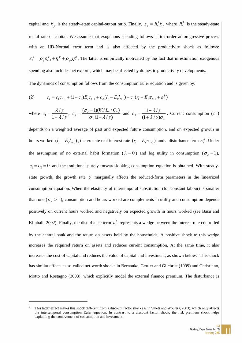
capital and is the steady-state capital-output ratio. Finally, where is the steady-state
rental rate of capital. We assume that exogenous spending follows a first-order autoregressive process
with an IID-Normal error term and is also affected by the productivity shock as follows:
. The latter is empirically motivated by the fact that in estimation exogenous
spending also includes net exports, which may be affected by domestic productivity developments.
yk yk
y kRz ∗= kR∗
atga
gt
gtg
gt ηρηερε ++= −1
The dynamics of consumption follows from the consumption Euler equation and is given by:
(2) )()()1( 13121111bttttttttttt ErclElccEcccc επ +−−−+−+= +++−
where γλ
γλ/1
/1 +=c ,
)/1()/)(1( ***
2 γλσσ
+−
=c
hc CLW
c and c
cσγλγλ)/1(
/13 +
−= . Current consumption ( )
depends on a weighted average of past and expected future consumption, and on expected growth in
hours worked , the ex-ante real interest rate
tc
)( 1+− ttt lEl )( 1+− ttt Er π and a disturbance term . Under
the assumption of no external habit formation (
btε
0=λ ) and log utility in consumption ( 1=cσ ),
and the traditional purely forward-looking consumption equation is obtained. With steady-
state growth, the growth rate
021 == cc
γ marginally affects the reduced-form parameters in the linearized
consumption equation. When the elasticity of intertemporal substitution (for constant labour) is smaller
than one ( 1>cσ ), consumption and hours worked are complements in utility and consumption depends
positively on current hours worked and negatively on expected growth in hours worked (see Basu and
Kimball, 2002). Finally, the disturbance term represents a wedge between the interest rate controlled
by the central bank and the return on assets held by the households. A positive shock to this wedge
increases the required return on assets and reduces current consumption. At the same time, it also
increases the cost of capital and reduces the value of capital and investment, as shown below.
btε
3 This shock
has similar effects as so-called net-worth shocks in Bernanke, Gertler and Gilchrist (1999) and Christiano,
Motto and Rostagno (2003), which explicitly model the external finance premium. The disturbance is
3 This latter effect makes this shock different from a discount factor shock (as in Smets and Wouters, 2003), which only affects
the intertemporal consumption Euler equation. In contrast to a discount factor shock, the risk premium shock helps explaining the comovement of consumption and investment.
11ECB
Working Paper Series No 722February 2007
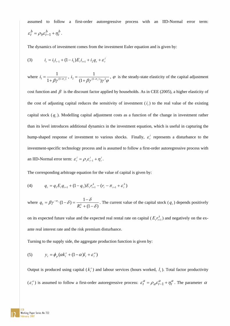
assumed to follow a first-order autoregressive process with an IID-Normal error term:
. bt
btb
bt ηερε += −1
The dynamics of investment comes from the investment Euler equation and is given by:
(3) itttttt qiiEiiii ε++−+= +− 21111 )1(
where )1(1 11
ci σβγ −+= ,
ϕγβγ σ 2)1(2 )1(1
ci −+= , ϕ is the steady-state elasticity of the capital adjustment
cost function and β is the discount factor applied by households. As in CEE (2005), a higher elasticity of
the cost of adjusting capital reduces the sensitivity of investment ( ) to the real value of the existing
capital stock ( ). Modelling capital adjustment costs as a function of the change in investment rather
than its level introduces additional dynamics in the investment equation, which is useful in capturing the
hump-shaped response of investment to various shocks. Finally, represents a disturbance to the
investment-specific technology process and is assumed to follow a first-order autoregressive process with
an IID-Normal error term: .
ti
tq
itε
it
iti
it ηερε += −1
The corresponding arbitrage equation for the value of capital is given by:
(4) )()1( 11111bttt
kttttt rrEqqEqq επ +−−−+= +++
where )1(
1)1(*
1 δδδβγ σ
−+−
=−= −kR
q c . The current value of the capital stock ( ) depends positively
on its expected future value and the expected real rental rate on capital ( ) and negatively on the ex-
ante real interest rate and the risk premium disturbance.
tq
ktt rE 1+
Turning to the supply side, the aggregate production function is given by:
(5) ))1(( att
stpt lky εααφ +−+=
Output is produced using capital ( ) and labour services (hours worked, ). Total factor productivity
( ) is assumed to follow a first-order autoregressive process: . The parameter
stk tl
atε
at
ata
at ηερε += −1 α
12ECB Working Paper Series No 722February 2007

captures the share of capital in production and the parameter pφ is one plus the share of fixed costs in
production, reflecting the presence of fixed costs in production.
As newly installed capital becomes only effective with a one-quarter lag, current capital services used in
production ( ) are a function of capital installed in the previous period ( ) and the degree of capital
utilisation ( ):
stk 1−tk
tz
(6) ttst zkk += −1
Cost minimisation by the households that provide capital services implies that the degree of capital
utilisation is a positive function of the rental rate of capital:
(7) ktt rzz 1=
where ψψ−
=1
1z and ψ is a positive function of the elasticity of the capital utilisation adjustment cost
function and normalized to be between zero and one. When 1=ψ , it is extremely costly to change the
utilisation of capital and as a result the utilisation of capital remains constant. In contrast, when 0=ψ ,
the marginal cost of changing the utilisation of capital is constant and as a result in equilibrium the rental
rate on capital is constant as is clear from equation (7).
The accumulation of installed capital ( ) is not only a function of the flow of investment but also of the
relative efficiency of these investment expenditures as captured by the investment-specific technology
disturbance:
tk
(8) itttt kikkkk ε2111 )1( +−+= −
with γδ /)1(1 −=k and . ϕγβγγδ σ 2)1(2 )1)(/)1(1( ck −+−−=
Turning to the monopolistic competitive goods market, cost minimisation by firms implies that the price
mark-up ( ), defined as the difference between the average price and the nominal marginal cost or the
negative of the real marginal cost, is equal to the difference between the marginal product of labour
( ) and the real wage ( ):
ptµ
tmpl tw
13ECB
Working Paper Series No 722February 2007

(9) tatt
sttt
pt wlkwmpl −+−=−= εαµ )(
As implied by the second equality in (9), the marginal product of labour is itself a positive function of the
capital-labour ratio and total factor productivity.
Due to price stickiness as in Calvo (1983) and partial indexation to lagged inflation of those prices that
can not be re-optimised as in Smets and Wouters (2003), prices adjust only sluggishly to their desired
mark-up. Profit maximisation by price-setting firms gives rise to the following New-Keynesian Phillips
curve:
(10) pt
pttttt E εµππππππ +−+= +− 31211
where p
p
cιβγι
π σ−+= 11 1
, p
c
c
ιβγβγπ σ
σ
−
−
+= 1
1
2 1 and
)1)1(()1)(1(
11 1
13 +−
−−
+=
−
−ppp
pp
p
c
c εφξξξβγ
ιβγπ
σ
σ . Inflation
( tπ ) depends positively on past and expected future inflation, negatively on the current price mark-up and
positively on a price mark-up disturbance ( ). The price mark-up disturbance is assumed to follow an
ARMA(1,1) process: , where is an IID-Normal price mark-up shock. The
inclusion of the MA term is designed to capture the high-frequency fluctuations in inflation.
ptε
ptp
pt
ptp
pt 1−−+= ηµηερε p
tη
When the degree of indexation to past inflation is zero ( 0=pι ), equation (10) reverts to a standard purely
forward-looking Phillips curve ( 01 =π ). The assumption that all prices are indexed to either lagged
inflation or the steady state inflation rate ensures that the Phillips curve is vertical in the long run. The
speed of adjustment to the desired mark-up depends among others on the degree of price stickiness ( pξ ),
the curvature of the Kimball goods market aggregator ( pε ) and the steady-state mark-up, which in
equilibrium is itself related to the share of fixed costs in production ( 1−pφ ) through a zero-profit
condition. A higher pε slows down the speed of adjustment because it increases the strategic
complementarity with other price setters. When all prices are flexible ( 0=pξ ) and the price-mark-up
shock is zero, equation (10) reduces to the familiar condition that the price mark-up is constant or
equivalently that there are no fluctuations in the wedge between the marginal product of labour and the
real wage.
Cost minimisation by firms will also imply that the rental rate of capital is negatively related to the
capital-labour ratio and positively to the real wage (both with unitary elasticity):
(11) tttk
t wlkr +−−= )(
14ECB Working Paper Series No 722February 2007

In analogy with the goods market, in the monopolistically competitive labour market the wage mark-up
will be equal to the difference between the real wage and the marginal rate of substitution between
working and consuming ( ): tmrs
(12) ))(1
1( 1−−−
+−=−= tttltttwt cclwmrsw λ
λσµ
where lσ is the elasticity of labour supply with respect to the real wage and λ is the habit parameter in
consumption.
Similarly, due to nominal wage stickiness and partial indexation of wages to inflation, real wages only
adjust gradually to the desired wage mark-up:
(13) wt
wttttttttt wwwEwEwwww εµπππ +−+−+−+= −++− 413211111 ))(1(
withc
w σβγ −+= 11 1
1,
c
cww σ
σ
βγιβγ
−
−
++
= 1
1
2 11
, c
ww σβγι
−+= 13 1
and )1)1((
)1)(1(1
1 1
14 +−−−
+=
−
−www
wwc
cw
εφξξξβγ
βγ
σ
σ .
The real wage is a function of expected and past real wages, expected, current and past inflation, the
wage mark-up and a wage-markup disturbance ( ). If wages are perfectly flexible (
tw
wtε 0=wξ ), the real
wage is a constant mark-up over the marginal rate of substitution between consumption and leisure. In
general, the speed of adjustment to the desired wage mark-up depends on the degree of wage stickiness
( wξ ) and the demand elasticity for labour, which itself is a function of the steady-state labour market
mark-up ( 1−wφ ) and the curvature of the Kimball labour market aggregator ( wε ). When wage
indexation is zero ( 0=wι ), real wages do not depend on lagged inflation ( ). The wage-markup
disturbance ( ) is assumed to follow an ARMA(1,1) process with an IID-Normal error term:
. As in the case of the price mark-up shock, the inclusion of an MA term
allows us to pick up some of the high frequency fluctuations in wages.
03 =w
wtε
wtw
wt
wtw
wt 11 −− −+= ηµηερε
4
Finally, the model is closed by adding the following empirical monetary policy reaction function:
(14) [ ] rt
ptt
ptty
pttYttt yyyyryyrrrr επρρ π +−−−+−+−+= −−∆− ))()()}(){1( 111
4 Alternatively, we could interpret this disturbance as a labour supply disturbance coming from changes in preferences for
leisure.
15ECB
Working Paper Series No 722February 2007

The monetary authorities follow a generalised Taylor rule by gradually adjusting the policy-controlled
interest rate ( ) in response to inflation and the output gap, defined as the difference between actual and
potential output (Taylor, 1993). Consistently with the DSGE model, potential output is defined as the
level of output that would prevail under flexible prices and wages in the absence of the two “mark-up”
shocks.
tr
5 The parameter ρ captures the degree of interest rate smoothing. In addition, there is also a
short-run feedback from the change in the output gap. Finally, we assume that the monetary policy
shocks ( ) follows a first-order autoregressive process with an IID-Normal error term:
.
rtε
rt
rtR
rt ηερε += −1
Equations (1) to (14) determine fourteen endogenous variables: , , , , , , , , , ty tc ti tq stk tk tz k
trp
tµ tπ ,
, , and . The stochastic behaviour of the system of linear rational expectations equations is
driven by seven exogenous disturbances: total factor productivity ( ), investment-specific technology
( ), risk premium ( ), exogenous spending ( ), price mark-up ( ), wage mark-up ( ) and
monetary policy ( ) shocks. Next we turn to the estimation of the model.
wtµ tw tl tr
atε
itε
btε
gtε
ptε
wtε
rtε
3. Parameter estimates
The model presented in the previous section is estimated with Bayesian estimation techniques using seven
key macro-economic quarterly US time series as observable variables: the log difference of real GDP,
real consumption, real investment and the real wage, log hours worked, the log difference of the GDP
deflator and the federal funds rate. A full description of the data used is given in the appendix. The
corresponding measurement equation is:
5 In practical terms, we expand the model consisting of equations (1) to (14) with a flexible-price-and-wage version in order to
calculate the model-consistent output gap. Note that the assumption of treating the wage equation disturbance as a wage mark-up disturbance rather than a labour supply disturbance coming from changed preferences has implications for our calculation of potential output.
16ECB Working Paper Series No 722February 2007

(15)
⎥⎥⎥⎥⎥⎥⎥⎥⎥
⎦
⎤
⎢⎢⎢⎢⎢⎢⎢⎢⎢
⎣
⎡
−−−−
+
⎥⎥⎥⎥⎥⎥⎥⎥⎥
⎦
⎤
⎢⎢⎢⎢⎢⎢⎢⎢⎢
⎣
⎡
=
⎥⎥⎥⎥⎥⎥⎥⎥⎥
⎦
⎤
⎢⎢⎢⎢⎢⎢⎢⎢⎢
⎣
⎡
=Υ −
−
−
−
t
t
t
tt
tt
tt
tt
t
t
t
t
t
t
t
t
r
lwwiiccyy
r
l
FEDFUNDSdlP
lHOURSdlWAGdlINV
dlCONSdlGDP
ππ
γγγγ
1
1
1
1
where and stand for log and log difference respectively, l dl )1(100 −= γγ is the common quarterly
trend growth rate to real GDP, consumption, investment and wages, )1(100 * −Π=π is the quarterly
steady-state inflation rate and )1(100 *1 −Π= − cr σγβ is the steady-state nominal interest rate. Given the
estimates of the trend growth rate and the steady-state inflation rate, the latter will be determined by the
estimated discount rate. Finally, l is steady-state hours-worked, which is normalized to be equal to zero.
First, we estimate the mode of the posterior distribution by maximising the log posterior function, which
combines the prior information on the parameters with the likelihood of the data. In a second step, the
Metropolis-Hastings algorithm is used to get a complete picture of the posterior distribution and to
evaluate the marginal likelihood of the model.6 The model is estimated over the full sample period from
1966:1 till 2004:4. In Section 5.4 we estimate the model over two subperiods (1966:1-1979:2 and 1984:1-
2004:4) in order to investigate the stability of the estimated parameters.7
6 See Smets and Wouters (2003) for a more elaborate description of the methodology. A sample of 250.000 draws was created
(neglecting the first 10.000 draws). The Hessian resulting from the optimisation procedure was used for defining the transition probability function that generates the new proposed draw. A step size of 0.3 resulted in a rejection rate of 0.65. The resulting sample properties are not sensitive to the step size. Two methods were used to test the stability of the sample. The difference between the means of the two sub-samples (100.000 first and 100.000 last drawings) should be Normal distributed with a standard error proportional to the square of the summed sub-sample variances divided by the sample size, if the draws are i.i.d. distributed. However the drawings of the MH algorithm are highly correlated. By selecting only each n drawing from the overall sample, the i.i.d. distribution is approximated. For bigger step sizes, the hypothesis of equality in mean of the two sub-samples can no longer be rejected for most of the parameters. The second method to evaluate the stability is a graphical test based on the cumulative mean minus the overall mean (see Bauwens et al, 2000). Starting from a minimal cumulative mean of 25.000 drawings, this ratio remains within a 10% band for all the parameters. In sum, an exact statistical test for the stability of the sample is complicated by the highly autocorrelated nature of the MH-sampler. However from an economic point of view the differences between subsamples and independent samples of size 100.000 or more are negligible.
7 The data set used generally starts in 1947. However, in previous versions of this paper we found that the first ten years are not representative of the rest of the sample, so that we decided to shorten the sample to 1957:1 – 2004:4. In addition, below in Section 4 we use the first 10 years as a training sample for calculating the marginal likelihood of unconstrained VARs, so that the effective sample starts in 1966:1.
17ECB
Working Paper Series No 722February 2007

3.1 Prior distribution of the parameters
The priors on the stochastic processes are harmonised as much as possible. The standard errors of the
innovations are assumed to follow an inverse-gamma distribution with a mean of 0.10 and two degrees of
freedom, which corresponds to a rather loose prior. The persistence of the AR(1) processes is beta
distributed with mean 0.5 and standard deviation 0.2. A similar distribution is assumed for the MA
parameter in the process for the price and wage mark-up. The quarterly trend growth rate is assumed to be
Normal distributed with mean 0.4 (quarterly growth rate) and standard deviation 0.1. The steady-state
inflation rate and the discount rate are assumed to follow a gamma distribution with a mean of 2.5% and
1% on an annual basis.
Five parameters are fixed in the estimation procedure. The depreciation rate δ is fixed at 0.025 (on a
quarterly basis) and the exogenous spending-GDP ratio is set at 18%. Both of these parameters would
be difficult to estimate unless the investment and exogenous spending ratios would be directly used in the
measurement equation. Three other parameters are clearly not identified: the steady-state mark-up in the
labour market (
yg
wλ ), which is set at 1.5, and the curvature parameters of the Kimball aggregators in the
goods and labour market ( pε and wε ), which are both set at 10.
The parameters describing the monetary policy rule are based on a standard Taylor rule: the long run
reaction on inflation and the output gap are described by a Normal distribution with mean 1.5 and 0.125
(0.5 divided by 4) and standard errors 0.125 and 0.05 respectively. The persistence of the policy rule is
determined by the coefficient on the lagged interest rate rate which is assumed to be Normal around a
mean of 0.75 with a standard error of 0.1. The prior on the short run reaction coefficient to the change in
the output-gap is 0.125.
The parameters of the utility function are assumed to be distributed as follows. The intertemporal
elasticity of substitution is set at 1.5 with a standard error of 0.375; the habit parameter is assumed to
fluctuate around 0.7 with a standard error of 0.1 and the elasticity of labour supply is assumed to be
around 2 with a standard error of 0.75. These are all quite standard calibrations. The prior on the
adjustment cost parameter for investment is set around 4 with a standard error of 1.5 (based on CEE,
2005) and the capacity utilisation elasticity is set at 0.5 with a standard error of 0.15. The share of fixed
18ECB Working Paper Series No 722February 2007

costs in the production function is assumed to have a prior mean of 0.25. Finally, there are the parameters
describing the price and wage setting. The Calvo probabilities are assumed to be around 0.5 for both
prices and wages, suggesting an average length of price and wage contracts of half a year. This is
compatible with the findings of Bils and Klenow (2004) for prices. The prior mean of the degree of
indexation to past inflation is also set at 0.5 in both goods and labour markets.8
3.2 Posterior estimates of the parameters
Table 1 gives the mode, the mean and the 5 and 95 percentiles of the posterior distribution of the
parameters obtained by the Metropolis-Hastings algorithm.
The trend growth rate is estimated to be around 0.43, which is somewhat smaller than the average growth
rate of output per capita over the sample. The posterior mean of the steady state inflation rate over the full
sample is about 3% on an annual basis. The mean of the discount rate is estimated to be quite small
(0.65% on an annual basis). The implied mean steady state nominal and real interest rates are respectively
about 6 % and 3% on an annual basis.
{Insert Table 1a-b}
A number of observations are worth making regarding the estimated processes for the exogenous shock
variables (Table 1b). Overall, the data appears to be very informative on the stochastic processes for the
exogenous disturbances. The productivity, the government spending and the wage mark-up processes are
estimated to be the most persistent with an AR(1) coefficient of 0.95, 0.97 and 0.96 respectively. The
mean of the standard error of the shock to the productivity process is 0.45. The high persistence of the
productivity and wage mark-up processes implies that at long horizons most of the forecast error variance
of the real variables will be explained by those two shocks. In contrast, both the persistence and the
standard deviation of the risk premium and monetary policy shock are relatively low (0.18 and 0.12
respectively).
Turning to the estimates of the main behavioural parameters, it turns out that the mean of the posterior
distribution is typically relatively close to the mean of the prior assumptions. There are a few notable
8 We have analysed the sensitivity of the estimation results to the prior assumptions by increasing the standard errors of the
prior distributions of the behavioural parameters by 50 %. Overall, the estimation results are very similar.
19ECB
Working Paper Series No 722February 2007

exceptions. Both the degree of price and wage stickiness are estimated to be quite a bit higher than 0.5.
The average duration of wage contracts is somewhat less than a year; whereas the average duration of
price contracts is about 3 quarters. The mean of the degree of price indexation (0.24) is on the other hand
estimated to be much less then 0.5.9 Also the elasticity of the cost of changing investment is estimated to
be higher than assumed a priori, suggesting an even slower response of investment to changes in the value
of capital. Finally, the posterior mean of the fixed cost parameter is estimated to be much higher than
assumed in the prior distribution (1.6) and the share of capital in production is estimated to be much lower
(0.19). Overall, it appears that the data is quite informative on the behavioural parameters as indicated by
the lower variance of the posterior distribution relative to the prior distribution. Two exceptions are the
elasticity of labour supply and the elasticity of the cost of changing the utilisation of capital, where the
posterior and prior distributions are quite similar.10
Finally, turning to the monetary policy reaction function parameters, the mean of the long-run reaction
coefficient to inflation is estimated to be relatively high (2.0). There is a considerable degree of interest
rate smoothing as the mean of the coefficient on the lagged interest rate is estimated to be 0.81. Policy
does not appear to react very strongly to the output gap level (0.09), but does respond strongly to changes
in the output-gap (0.22) in the short run.
4. Forecast performance: comparison with VAR models
In this Section we compare the out-of-sample forecast performance of the estimated DSGE model with
that of various VARs estimated on the same data set. The marginal likelihood, which can be interpreted as
a summary statistic for the model’s out-of-sample prediction performance, forms a natural benchmark for
comparing the DSGE model with alternative specifications and other statistical models.11 However, as
9 When relaxing the prior distributions, it turns out that the degree of wage stickiness rise even more, whereas the degree of
price indexation falls by more. 10 Figures with the prior and posterior distributions of all the parameters are available upon request. 11 As discussed in Geweke (1998), the Metropolis-Hastings-based sample of the posterior distribution can be used to evaluate
the marginal likelihood of the model. Following Geweke (1998), we calculate the modified harmonic mean to evaluate the integral over the posterior sample. An alternative approximation is the Laplace approximation around the posterior mode, which is based on a normal distribution. In our experience the results of both approximations are very close in the case of our estimated DSGE model. This is not too surprising given the generally close correspondence between the histograms of the posterior sample and the normal distribution around the estimated mode for the individual parameters. Given the large advantage of the Laplace approximation in terms of computational costs, we will use this approximation for comparing alternative model specifications in the next section.
20ECB Working Paper Series No 722February 2007
Sims (2003) has pointed out it is important to use a training sample in order to standardize the prior
distribution across widely different models. In order to check for robustness, we also consider a more
traditional out-of-sample RMSE forecast exercise in this section.
{Insert Table 2}
Table 2 compares the marginal likelihood of the DSGE model and various unconstrained VAR models,
all estimated over the full sample period (1966:1 – 2004:4) and using the period 1956:1 – 1965:4 as a
training sample. Several results are worth emphasizing. First, the tightly parameterized DSGE model
performs much better than an unconstrained VAR in the same vector of observable variables, tΥ (first
column of Table 2). The bad empirical performance of unconstrained VARs may not be too surprising, as
it is known that over-parameterized models typically perform poorly in out-of-sample forecast exercises.
One indication of this is that the marginal likelihood of the unconstrained VAR model deteriorates
quickly as the lag order increases. For that reason, in the second column of Table 2, we consider the
Bayesian VAR model proposed by Sims and Zha (1998). This BVAR combines a Minnesota-type prior
(see Litterman, 1984) with priors that take into account the degree of persistence and cointegration in the
variables. In order to allow the data to decide on the degree of persistence and cointegration, in this
BVAR we enter real GDP, consumption, investment and the real wage in log levels. When setting the
tightness of the prior, we choose a set of parameters recommended by Sims (2003) for quarterly data.12
The second column of Table 2 shows that the marginal likelihood of the Sims-Zha BVAR increases
significantly compared to the unconstrained VAR. Moreover, the best BVAR model (BVAR(4)) does as
well as the DSGE model.13
Overall, the comparison of marginal likelihoods shows that the estimated DSGE model can compete with
standard BVAR models in terms of empirical one-step-ahead prediction performance. These results are
confirmed by a more traditional out-of sample forecasting exercise reported in Table 3. Table 3 reports
out-of-sample RMSEs for different forecast horizons over the period 1990:1 to 2004:4. For this exercise,
12 In order to determine the tightness of the priors, we use standard values as suggested in Sims (2003) (See also Sims and Zha,
1998). In particular, the decay parameter is set at 1.0, the overall tightness is set at 10, the parameter determining the weight on the "sum of coefficients" or "own-persistence" is set at 2.0 and the parameter determining the weight on the "co-persistence" at 5. Moreover, the vector of prior standard deviations of the equation shocks is based on the VAR(1) residuals estimated over the training period.
21ECB
Working Paper Series No 722February 2007

the VAR(1), BVAR(4) and DSGE model were initially estimated over the sample 1966:1 - 1989:4. The
models were then used to forecast the seven data series contained in tΥ from 1990:1 to 2004:4, whereby
the VAR(1) and BVAR(4) models were re-estimated every quarter, whereas the DSGE model was re-
estimated every year. The measure of overall performance reported in the last column of Table 3 is the
log determinant of the uncentered forecast error covariance matrix.
{Insert Table 3}
The out-of-sample forecast statistics confirm the good forecast performance of the DSGE model relative
to the VAR and BVAR models. At the one-quarter ahead horizon, the BVAR(4) and the DSGE model
improve with about the same magnitude over the VAR(1) model, confirming the results from Table 2.
However, over longer horizons up to three years, the DSGE model does considerably better than both the
VAR(1) and BVAR(4) model. Somewhat surprisingly, the BVAR(4) model performs worse than the
simple VAR(1) model at longer horizons. Moreover, the improvement appears to be quite uniform across
the seven macro variables.
5. Model sensitivity: which frictions are empirically important?
The introduction of a large number of frictions raises the question which of those are really necessary to
capture the dynamics of the data. In this Section we examine the contribution of each of the frictions to
the marginal likelihood of the DSGE model.
Table 4 presents the estimates of the mode of the parameters and the marginal likelihood when each of
frictions (price and wage stickiness, price and wage indexation, investment adjustment costs and habit
formation, capital utilisation and fixed costs in production) are drastically reduced one at a time. This
table also gives an idea of the robustness of the parameters and the model performance with respect to the
various frictions included in the model. For comparison, the first column reproduces the baseline
estimates (mode of the posterior) and the marginal likelihood based on the Laplace approximation.
{Insert Table 4}
13 The marginal likelihood can be further increased by optimising the tightness of the “own persistence” prior. For example,
setting this parameter equal to 10 increases the marginal likelihood of the BVAR(4) model to -896.
22ECB Working Paper Series No 722February 2007
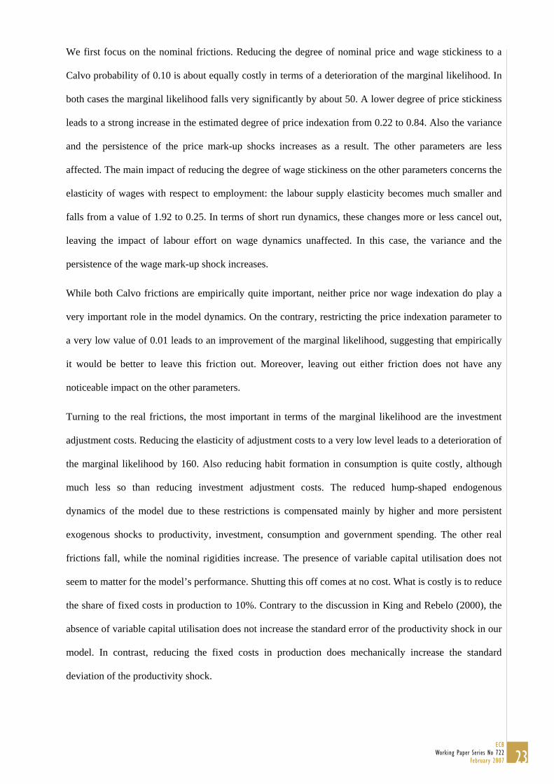
We first focus on the nominal frictions. Reducing the degree of nominal price and wage stickiness to a
Calvo probability of 0.10 is about equally costly in terms of a deterioration of the marginal likelihood. In
both cases the marginal likelihood falls very significantly by about 50. A lower degree of price stickiness
leads to a strong increase in the estimated degree of price indexation from 0.22 to 0.84. Also the variance
and the persistence of the price mark-up shocks increases as a result. The other parameters are less
affected. The main impact of reducing the degree of wage stickiness on the other parameters concerns the
elasticity of wages with respect to employment: the labour supply elasticity becomes much smaller and
falls from a value of 1.92 to 0.25. In terms of short run dynamics, these changes more or less cancel out,
leaving the impact of labour effort on wage dynamics unaffected. In this case, the variance and the
persistence of the wage mark-up shock increases.
While both Calvo frictions are empirically quite important, neither price nor wage indexation do play a
very important role in the model dynamics. On the contrary, restricting the price indexation parameter to
a very low value of 0.01 leads to an improvement of the marginal likelihood, suggesting that empirically
it would be better to leave this friction out. Moreover, leaving out either friction does not have any
noticeable impact on the other parameters.
Turning to the real frictions, the most important in terms of the marginal likelihood are the investment
adjustment costs. Reducing the elasticity of adjustment costs to a very low level leads to a deterioration of
the marginal likelihood by 160. Also reducing habit formation in consumption is quite costly, although
much less so than reducing investment adjustment costs. The reduced hump-shaped endogenous
dynamics of the model due to these restrictions is compensated mainly by higher and more persistent
exogenous shocks to productivity, investment, consumption and government spending. The other real
frictions fall, while the nominal rigidities increase. The presence of variable capital utilisation does not
seem to matter for the model’s performance. Shutting this off comes at no cost. What is costly is to reduce
the share of fixed costs in production to 10%. Contrary to the discussion in King and Rebelo (2000), the
absence of variable capital utilisation does not increase the standard error of the productivity shock in our
model. In contrast, reducing the fixed costs in production does mechanically increase the standard
deviation of the productivity shock.
23ECB
Working Paper Series No 722February 2007

Overall, the results from this sensitivity exercise illustrate that the estimated parameters appear relatively
robust to changes in the frictions one by one. Price and wage indexation and variable capital utilisation
are of minor importance in terms of the overall empirical performance of the model. On the real side,
investment adjustment costs are the most important friction. On the nominal side, both wage and price
stickiness are very important.
6. Applications
After having shown that the estimated model fits the US macro-economic data quite well, we use it to
investigate a number of key macro-economic issues. In this section, we address the following questions.
First, what are the main driving forces of output? Second, can the model replicate the cross correlation
between output and inflation? Third, what is the effect of a productivity shock on hours worked? Fourth,
why have output and inflation become less volatile? We study these issues in each subsection in turn.
6.1 What are the main driving forces of output?
Figure 1 gives the forecast error variance decomposition of output, inflation and the federal funds rate at
various horizons based on the mode of the model’s posterior distribution reported in Section 3. In the
short run (within a year) movements in real GDP are primarily driven by the exogenous spending shock
and the two shocks that affect the intertemporal Euler equations, i.e. the risk premium shock which affects
both the consumption and investment Euler equation and the investment-specific technology shock which
affects the investment Euler equation. Together they account for more than 50 percent of the forecast
error variance of output up to one year. Each of those shocks can be categorised as “demand” shocks in
the sense that they have a positive effect on output, hours worked, inflation and the nominal interest rate
under the estimated policy rule. This is illustrated in Figure 2 which shows the estimated mean impulse
response functions to each of those three shocks. Not surprisingly, the risk premium shock explains a big
part of the short-run variations in consumption, while the investment shock explains the largest part of
investment in the short run (not shown).14
{Insert Figure 1}
24ECB Working Paper Series No 722February 2007

{Insert Figure 2}
However, in line with the results of Shapiro and Watson (1989), it is mostly two “supply” shocks, the
productivity and the wage mark-up shock, that account for most of the output variations in the medium to
long run. Indeed, even at the two year horizon, together the two shocks account for more than 50% of the
variations in output. In the longer run, the wage mark-up shock dominates the productivity shock. Those
shocks also become dominant forces in the long-run developments of consumption and to a lesser extent
investment. Not surprisingly, the wage-markup shock is also the dominant factor behind long-run
movements in hours worked. As shown in Figure 3, a typical positive wage mark-up shock gradually
reduces output and hours worked by 0.8 and 0.6 percent respectively. Confirming the large identified
VAR literature on the role of monetary policy shocks (e.g. Christiano, Eichenbaum and Evans, 2000),
monetary policy shocks contribute only a small fraction of the forecast variance of output at all horizons.
{Insert Figure 3}
Figure 4 shows the historical contribution of each of four types of shocks (productivity, demand,
monetary policy and mark-up shocks) to annual output growth over the sample period. It is interesting to
compare the main sources of the various recessions over this period. While the recessions of the early
1990s and the beginning of the new millennium are mainly driven by demand shocks, the recession of
1974 is mainly due to positive mark-up shocks (associated with the oil crisis). Monetary policy shocks
only play a dominant role in the recession of the early 1980s when the Federal Reserve under the
chairmanship of Paul Volker started the disinflation process.
{Insert Figure 4}
6.2 Determinants of inflation and the output-inflation cross correlation?
Figure 1 also contains the variance decomposition of inflation. It is quite clear that at all horizons, price
and wage mark-ups are the most important drivers of inflation. In the short run, price mark-ups dominate,
whereas in the medium to long run wage mark-ups become relatively more important. Even at the
medium to long-run horizons, the other shocks only explain a minor fraction of the total variation in
inflation. Similarly, monetary policy shocks account for only a small fraction of inflation volatility. This
14 The full set of impulse response functions, as well as the associated confidence sets, are available in the appendix on request.
25ECB
Working Paper Series No 722February 2007

is also clear from Figure 4, which depicts the historical contribution of the different types of shocks to
inflation over the sample period. The dominant source of secular shifts in inflation is driven by price and
wage mark-up shocks. However, also monetary policy did play a role in the rise of inflation in the 1970s
and the subsequent disinflation during the Volker period. Moreover, negative demand shocks did
contribute to low inflation in the early 1990s and the start of the new millennium.
There are at least two reasons why the various demand and productivity shocks have only limited effects
on inflation. First, the estimated slope of the New Keynesian Phillips curve is very small, so that only
large and persistent changes in the marginal cost will have an impact on inflation. Second, and more
importantly, under the estimated monetary policy reaction function the Fed responds quite aggressively to
emerging output gaps and their impact on inflation. This is reflected in the fact that at the short and
medium-term horizon more than 60 percent of variations in the nominal interest rate are due to the
various demand and productivity shocks, in particular the risk premium shock (third panel of Figure 1).
Only in the long run, does the wage mark-up shock become a dominant source of movements in nominal
interest rates.
{Insert Figure 5}
In the light of these results it is interesting to see to what extent our model can replicate the empirical
correlation function between output and inflation as, for example, highlighted in Gali and Gertler (1999).
Figure 5 plots the empirical correlation function of output (detrended using the Hodrick-Prescott filter)
and inflation (estimated over the period 1966:1-2004:4), as well as the median and the 5 and 95%
equivalent generated by the model’s posterior distribution. In order to generate this distribution, 1000
draws from the posterior distribution of the model parameters are used to generate artificial samples of
output and inflation of the same sample size as the actual data set. For each of those 1000 artificial
samples, the autocorrelation function is calculated and the median and 5 and 95 percentiles are derived.
Figure 5 clearly shows that the DSGE model is able to replicate both the negative correlation between
inflation one to two years in the past and current output and the positive correlation between current
output and inflation one year ahead. Moreover, the correlations generated by the DSGE model are
significantly different from zero. Decomposing the cross-covariance function in contributions by the
different types of shocks, we find that the negative correlation between current inflation and future output
26ECB Working Paper Series No 722February 2007

is mostly driven by the price and wage mark-up shocks. In contrast, the positive correlation between the
current output gap and future inflation is the result of both demand shocks and mark-up shocks. Monetary
policy shocks do not play a role for two reasons. First, they account for only a small fraction of inflation
and output developments. Second, as shown in Figure 6, according to the estimated DSGE model the
peak effect of a policy shock on inflation occurs before its peak effect on output.
{Insert Figure 6}
6.3 The effect of a productivity shock on hours worked
Following Galí (1999), there has been a lively debate about the effects of productivity shocks on hours
worked and about the implications of this finding for the role of those shocks in US business cycles. Galí
(1999), Francis and Ramey (2005) and Galí and Rabanal (2004) have argued that due to the presence of
nominal price rigidities, habit formation and adjustment costs to investment, positive productivity shocks
lead to an immediate fall in hours worked. Given the strongly positive correlation between output and
hours worked over the business cycle this implies that productivity shocks can not play an important role
in the business cycle. In contrast, using alternative VAR specifications and identification strategies,
Christiano et al (2004), Dedola and Neri (2004) and Peersman and Straub (2005) have argued that the
empirical evidence on the effect of a productivity shock on hours worked is not very robust and could be
consistent with a positive impact on hours worked.
{Insert Figure 7}
In Section 6.1 we have already discussed that productivity shocks play an important, but not dominant
role in driving output developments beyond the one year horizon in our estimated model. At business
cycle frequencies, they account for about 25 to 30% of the forecast error variance. Figure 7 presents the
response of the actual and the flexible-price level of output, hours worked and nominal interest rate to a
productivity shock in the estimated model. Overall, the estimates confirm the analysis of Gali (1999) and
Francis and Ramey (2004). A positive productivity shock leads to an expansion of aggregate demand,
output and real wages, but an immediate and significant reduction in hours worked. Hours worked turn
27ECB
Working Paper Series No 722February 2007

only significantly positive after two years.15 Under the estimated monetary policy reaction function,
nominal and real interest rates fall, but not enough to prevent the opening up of an output gap and a fall in
inflation. Moreover, our estimation results show that it is mainly the estimated degree of habit persistence
and the importance of capital adjustment costs that explain the negative impact of productivity on hours
worked, thereby confirming the analysis of Francis and Ramey (2004). Indeed, also under flexible prices,
hours worked would fall significantly as indicated in the upper right-hand panel of Figure 7. Given these
estimates, it is unlikely that a more accommodative monetary policy would lead to positive employment
effects. The relatively low medium-run positive effects on hours worked are due to two factors. First,
although persistent, the productivity shock is temporary. As a result, output already starts returning to
baseline when the effects on hours worked start materialising. A different stochastic process for the
productivity shock which implies a gradual introduction of higher total factor productivity could increase
the effect on hours worked.16 Second, a positive productivity shock reduces the fixed cost per unit of
production and therefore less labour is required for a given output.
6.4 The “Great Inflation” and the “Great Moderation”: sub-sample estimates
In this Section we first compare the estimates for two sub-samples in order to investigate the stability of
the full-sample estimates and then examine using those estimates why output and inflation volatility has
fallen in the most recent period. The first sub-sample, corresponding to the period 1966:2-1979:2,
captures the period of the “Great Inflation” and ends with the appointment of Paul Volcker as chairman of
the Federal Reserve Board. The second sub-sample, 1984:1-2004:4 captures the more recent period of the
“Great Moderation”, in which not only inflation was relatively low and stable, but also output and
inflation volatility fell considerably (e.g. McConnell and Perez-Quiros, 2000). Table 5 compares the
mode of the posterior distribution of the DSGE model parameters over both periods.
{Insert Table 5}
The most significant differences between the two sub-periods concern the variances of the stochastic
processes. In particular the standard errors of the productivity, monetary policy and price mark-up shocks
15 This picture does not change very much when we do not allow for a positive effect of productivity on exogenous spending 16 See for instance Rotemberg (2003) for arguments favoring a slow appearance of major productivity advances in output
growth.
28ECB Working Paper Series No 722February 2007

(and to a lesser extent the investment shock) seem to have fallen. The persistence of those processes has
changed much less. One exception is the risk premium shock which has become even less persistent in
the second sub-period.
Somewhat surprisingly, the steady state inflation rate is only marginally lower in the second subperiod
(2.6) versus the first period (2.9). What is different is the central bank’s reaction coefficient to the output
gap, which is halved and is no longer significant in the second period. In contrast, the response to
inflation is only marginally higher in the second period and the response to the change in the output gap is
the same. These results are consistent with the findings of Orphanides (2003), who shows using real-time
data estimates that what has changed in US monetary policy behaviour since the early 1980s is the
relative response to output. They are, however, at odds with the results of Boivin and Giannoni (2006),
which finds that a stronger central bank response to inflation in the second subperiod can account for a
smaller output response to monetary policy shocks estimated in identified VARs. In our case, the lower
response to the output gap actually increases the output response of a monetary policy shock in the second
period.
Interestingly, it turns out that the degree of price and wage stickiness has increased in the second period,
while the degree of indexation has fallen. The latter is consistent with single-equation sub-sample
estimates of a hybrid New Keynesian Phillips curve by Gali and Gertler (1999). This finding is also
consistent with the story that low and stable inflation may reduce the cost of not adjusting prices and
therefore lengthen the average price duration leading to a flatter Phillips curve. At the same time, it may
also reduce rule-of-thumb behaviour and indexation leading to a lower coefficient on lagged inflation in
the Phillips curve. The effects are most visible in the goods market, less in the labour market. Finally,
there is also some limited evidence of increased real rigidities in the second sub-sample. For example, the
elasticity of adjusting capital increases from 3.6 to 6.4 in the second sub-sample.
{Insert Table 6}
In order to assess, the sources behind the great moderation of the last two decades, Table 6 provides the
results of a counterfactual exercise in which we examine what the standard deviation of output growth
and inflation would have been in the most recent period if the US economy had faced the same shocks as
in the 1970s, if the monetary policy reaction function as estimated in the pre-1979 period would have
29ECB
Working Paper Series No 722February 2007

been the same, or if the structure of the economy would have remained unchanged. Table 6 first of all
confirms that both output growth and inflation were significantly less volatile in the second sub sample.
The estimated DSGE model captures this reduction in volatility, although it overestimates the standard
deviation somewhat in both periods. Turning to the counterfactual exercise, it turns out that the most
important drivers behind the reduction in volatility are the shocks, which appear to have been more
benign in the last period. A reversal to the monetary policy reaction function of the 1970s would have
contributed to somewhat higher inflation volatility and lower output growth volatility, but these effects
are very small compared to the overall reduction in volatility. Finally, also the changes in the structural
parameters do not appear to have contributed to a major change in the volatility of the economy. Overall,
these results appear to confirm recent findings of Stock and Watson (2003) and Sims and Zha (2006) that
most of the structural change can be assigned to changes in the volatility of the shocks. It remains an
interesting research question whether policy has contributed to the reduction of those shocks.
7. Concluding remarks
In this paper, we have shown that modern micro-founded NNS models are able to fit the main US macro
data very well, if one allows for a sufficiently rich stochastic structure and set of frictions. Our results
support the earlier approaches by Rotemberg and Woodford (1997) and Christiano, Eichenbaum and
Evans (2005). Although the estimated structural model is highly restricted, it is able to compete with
standard VAR and BVAR models in out-of-sample forecasting, indicating that the theory embedded in
the structural model is helpful in improving the forecasts of the main US macro variables, in particular at
business cycle frequencies.
Of course, the estimated model remains stylised and should be further developed. In particular, a deeper
understanding of the various nominal and real frictions that have been introduced would increase the
confidence in using this type of models for welfare analysis. Our analysis also raises questions about the
deeper determinants of the various “structural” shocks such as productivity and wage mark-up shocks that
are identified as being important driving factors of output and inflation developments? However, we hope
to have shown that the Bayesian approach followed in this paper offers an effective tool for comparing
and selecting between such alternative micro-founded model specifications.
30ECB Working Paper Series No 722February 2007

References
Altig, D., L. Christiano, M. Eichenbaum and J. Linde (2004), „Firm-specific capital, nominal rigidities
and the business cycle”, mimeo, Northwestern University.
Basu, S. and M. Kimball (2002), “Long-run labour supply and the elasticity of intertemporal substitution
for consumption”, mimeo, University of Michigan.
Bauwens, L., M. Lubrano and J.F. Richards (2000), Bayesian inference in dynamic econometric models,
Oxford University Press.
Bernanke, B., Gertler, M. and S. Gilchrist (1999), “The financial accelerator in a quantitative business
cycle framework” in J. Taylor and M. Woodford (eds.), Handbook of Macroeconomics, Amsterdam:
North Holland.
Bils, M. and P. Klenow (2004), “Some evidence on the importance of price stickiness”, Journal of
Political Economy, 112(5), 947-986.
Boivin, J. and M. Giannoni (2006), “Has monetary policy become more effective?”, CEPR Discussion
Paper 5463.
Calvo, G. (1983), “Staggered prices in a utility maximising framework”, Journal of Monetary Economics.
Chang, Y., J. Gomes and F. Schorfheide (2002), ”Learning-by-Doing as Propagation Mechanism",
American Economic Review, 92(5), 1498-1520.
Christiano, L., M. Eichenbaum and C. Evans (2000), “Monetary policy shocks: what have we learned and
to what end”, in: M. Woodford and J. Taylor (eds.), Handbook of Macroeconomics, Amsterdam: North
Holland.
Christiano, L.J., Eichenbaum, M. and C. Evans (2005), “Nominal rigidities and the dynamic effects of a
shock to monetary policy”, Journal of Political Economy, 113(1), 1-46.
Christiano, L., M. Eichenbaum and R. Vigfusson (2004), „What happens after a technology shock?”,
mimeo, Northwestern University.
Christiano, L., R. Motto and M. Rostagno (2003), “The Great Depression and the Friedman-Schwartz
hypothesis”, Journal of Money, Credit and Banking, 35(6, part 2), 1119-1197.
31ECB
Working Paper Series No 722February 2007

Clarida, R., Gali, J. and M. Gertler (1999), “The science of monetary policy: a new Keynesian
Perspective”, Journal of Economic Literature, 37:4, p. 1661-1707.
Dedola, L. and S. Neri (2004), “What does a technology shock do? A VAR analysis with model-based
sign restrictions”, CEPR Working Paper 4537.
Eichenbaum, M. and J. Fisher (forthcoming), “Estimating the frequency of reoptimisation in Calvo-style
models”, forthcoming in Journal of Monetary Economics.
Francis, N. and V. Ramey (2005), “Is the technology-driven real business cycle hypothesis dead? Shocks
and aggregate fluctuations revisited”, Journal of Monetary Economics, 52:8 (November), 1379-1399.
Gali, J. (1999), “Technology, employment, and the business cycle: do technology shocks explain
aggregate fluctuations?” American Economic Review, 89(1), 249-271.
Gali, J. and Mark Gertler (1999), "Inflation Dynamics: A Structural Econometric Analysis", Journal of
Monetary Economics, 37(4), pp. 195-222.
Galí, J. and P. Rabanal (2004), “Technology shocks and aggregate fluctuations: How well does the RBC
model fit post-war US data?”, NBER Macroeconomics Annual 2004, 225-288.
Geweke, J. (1998), “Using simulation methods for Bayesian econometric models: inference, development
and communication”, mimeo, University of Minnesota and Federal Reserve Bank of Minneapolis.
Goodfriend, M and R. King (1997), “The new neoclassical synthesis and the role of monetary policy”, in:
Bernanke, B. and J. Rotemberg (eds), NBER Macroeconomics Annual 1997, 231-283.
Kimball, M. (1995), “The quantitative analytics of the basic neomonetarist model”, Journal of Money,
Credit and Banking, 27(4), Part 2, 1241-1277.
King, R.G. and S. Rebelo (2000), "Resuscitating real business cycles", in J. Taylor and M. Woodford
(eds), Handbook of macroeconomics, North Holland, 927-1007.
Litterman, R. (1984), “Forecasting and policy analysis with Bayesian Vector Autoregresssion models”,
Federal Reserve Bank of Minneapolis Quarterly Review, 8(4), 30-41.
Mc Connell, M. and G. Perez-Quiros (2000), “Output fluctuations in the US: What has changed since the
early 1980s?”, American Economic Review 90(5), December.
32ECB Working Paper Series No 722February 2007

Orphanides, A. (2003), "Historical monetary policy analysis and the Taylor rule", Journal of Monetary
Economics, 50(5), 983-1022.
Peersman, G. and R. Straub (2005), “Technology shocks and robust sign restrictions in a euro area
SVAR”, ECB Working Paper 373 (July).
Rotemberg, J. and M. Woodford (1997), “An optimization-based econometric framework for the
evaluation of monetary policy”, NBER Macroeconomics Annual 1997, Eds: B. Bernanke and J.
Rotemberg, Cambridge: MIT Press.
Rotemberg, J. "Stochastic technical progress, smooth trends, and nearly distinct business cycles."
American Economic Review, 93:5 (December 2003), 1543-1559
Shapiro, M.D. and J. Watson (1988), “Sources of Business Cycle Fluctuations”, NBER Macroeconomics
Annual, 1988, p. 111-148.
Sims, C. and T. Zha (2006), “Were there regime switches in US monetary policy?”, American Economic
Review 96(1), 54-82.
Sims, C. and T. Zha (1998), “Bayesian methods for dynamic multivariate models”, International
Economic Review 39, 949-968.
Sims, C. (2003), “Probability models for monetary policy decisions”, mimeo, Princeton University.
Smets, F. and R. Wouters (2003), “An estimated dynamic stochastic general equilibrium model of the
euro area”, Journal of the European Economic Association, 1:5 (September), 1123-1175.
Smets, F. and R. Wouters (2005), “Comparing shocks and frictions in US and euro area business cycles: a
Bayesian DSGE approach”, Journal of Applied Econometrics, 20:1 (January).
Stock, J. and M. Watson (2003), “Has the business cycle changed? Evidence and explanations”, in:
Monetary policy and uncertainty, Federal Reserve Bank of Kansas City, 9-56.
Taylor, J. (1993), “Discretion versus policy rules in practice”, Carnegie-Rochester Conference Series on
Public Policy 39, 195-214.
Woodford M. (2003), Interest and prices, Princeton University Press.
33ECB
Working Paper Series No 722February 2007

Table 1a: Prior and posterior distribution of structural parameters
Prior distribution Posterior distribution
Distr. Mean St.Dev. Mode Mean 5% 95%
ϕ Normal 4.00 1.50 5.48 5.74 3.97 7.42
cσ Normal 1.50 0.37 1.39 1.38 1.16 1.59
h Beta 0.70 0.10 0.71 0.71 0.64 0.78
wξ Beta 0.50 0.10 0.73 0.70 0.60 0.81
Lσ Normal 2.00 0.75 1.92 1.83 0.91 2.78
pξ Beta 0.50 0.10 0.65 0.66 0.56 0.74
wι Beta 0.50 0.15 0.59 0.58 0.38 0.78
pι Beta 0.50 0.15 0.22 0.24 0.10 0.38
ψ Beta 0.50 0.15 0.54 0.54 0.36 0.72
Φ Normal 1.25 0.12 1.61 1.60 1.48 1.73
πr Normal 1.50 0.25 2.03 2.04 1.74 2.33
ρ Beta 0.75 0.10 0.81 0.81 0.77 0.85
yr Normal 0.12 0.05 0.08 0.08 0.05 0.12
yr∆ Normal 0.12 0.05 0.22 0.22 0.18 0.27
π Gamma 0.62 0.10 0.81 0.78 0.61 0.96
100( ) 11 −−β Gamma 0.25 0.10 0.16 0.16 0.07 0.26
L Normal 0.00 2.00 -0.1 0.53 -1.3 2.32
γ Normal 0.40 0.10 0.43 0.43 0.40 0.45
α Normal 0.30 0.05 0.19 0.19 0.16 0.21
Note: The posterior distributions is obtained using the Metropolis-Hastings algorithm
34ECB Working Paper Series No 722February 2007

Table 1b: Prior and posterior distribution of shock processes
Prior distribution Posterior distribution
Distr. Mean St.Dev. Mode Mean 5% 95%
aσ Invgamma 0.10 2.00 0.45 0.45 0.41 0.50
bσ Invgamma 0.10 2.00 0.24 0.23 0.19 0.27
gσ Invgamma 0.10 2.00 0.52 0.53 0.48 0.58
Iσ Invgamma 0.10 2.00 0.45 0.45 0.37 0.53
rσ Invgamma 0.10 2.00 0.24 0.24 0.22 0.27
pσ Invgamma 0.10 2.00 0.14 0.14 0.11 0.16
wσ Invgamma 0.10 2.00 0.24 0.24 0.20 0.28
aρ Beta 0.50 0.20 0.95 0.95 0.94 0.97
bρ Beta 0.50 0.20 0.18 0.22 0.07 0.36
gρ Beta 0.50 0.20 0.97 0.97 0.96 0.99
Iρ Beta 0.50 0.20 0.71 0.71 0.61 0.80
rρ Beta 0.50 0.20 0.12 0.15 0.04 0.24
pρ Beta 0.50 0.20 0.90 0.89 0.80 0.96
wρ Beta 0.50 0.20 0.97 0.96 0.94 0.99
pµ Beta 0.50 0.20 0.74 0.69 0.54 0.85
wµ Beta 0.50 0.20 0.88 0.84 0.75 0.93
gaρ Beta 0.50 0.20 0.52 0.52 0.37 0.66
Note: The posterior distribution is obtained using the Metropolis-Hastings algorithm.
35ECB
Working Paper Series No 722February 2007

Table 2: Comparison of the marginal likelihood of alternative VAR models and the DSGE model
Order of the VAR No other prior Sims and Zha (1998) prior
VAR(1) -928.0 -940.9
VAR(2) -966.6 -915.8
VAR(3) -1018.1 -908.7
VAR(4) -1131.2 -906.6
VAR(5) - -907.7
Memo: DSGE model -905.8 -905.8
Note: In order to increases the comparability of the marginal likelihood of the various models, all models
are estimated using the period 1956:1-1965:4 as a training sample (Sims, 2002).
36ECB Working Paper Series No 722February 2007

Table 3: Out-of-sample prediction performance
GDP dP Fedfunds Hours Wage CONS INV Overall
VAR(1) RMSE-statistic for different forecast horizons
1q 0.60 0.25 0.10 0.46 0.64 0.60 1.62 -12.87
2q 0.94 0.27 0.18 0.78 1.02 0.95 2.96 -8.19
4q 1.64 0.34 0.36 1.45 1.67 1.54 5.67 -3.25
8q 2.40 0.53 0.64 2.13 2.88 2.27 8.91 1.47
12q 2.78 0.63 0.79 2.41 4.09 2.74 10.97 2.36
BVAR(4) Percentage gains (+) or losses (-) relative to VAR(1) model
1q 2.05 14.14 -1.37 -3.43 2.69 12.12 2.54 3.25
2q -2.12 15.15 -16.38 -7.32 -0.29 10.07 2.42 0.17
4q -7.21 31.42 -12.61 -8.58 -3.82 1.42 0.43 0.51
8q -15.82 33.36 -13.26 -13.94 -8.98 -8.19 -11.58 -4.10
12q -15.55 37.59 -13.56 -4.66 -15.87 -3.10 -23.49 -9.84
DSGE Percentage gains (+) or losses (-) relative to VAR(1) model
1q 5.68 2.05 -8.24 0.68 5.99 20.16 9.22 3.06
2q 14.93 10.62 -17.22 10.34 6.20 25.85 16.79 2.82
4q 20.17 46.21 1.59 19.52 9.21 26.18 21.42 6.82
8q 22.55 68.15 28.33 22.34 15.72 21.82 25.95 11.50
12q 32.17 74.15 40.32 27.05 21.88 23.28 41.61 13.51
Notes: All models are estimated starting in 1966:1. The forecast period is 1990:1-2004:4. VAR(1) and BVAR(4) models are re-estimated each quarter; the DSGE model each year. The overall measure of forecast performance is the log determinant of the uncentered forecast error covariance matrix. Gains and losses in the overall measure are expressed as the difference in the overall measure divided by the number of variables and by two to convert the variance to standard errors (times 100).
37ECB
Working Paper Series No 722February 2007

Table 4: Testing the empirical importance of the nominal and real frictions in the DSGE model
Base 1.0=pξ 1.0=wξ 0.0=pι 0.0=wι 1.0=ϕ 1.0=h 99.0=ψ 1.1=Φ
Marginal likelihood
-923 -975 -973 -918 -927 -1084 -959 -924 -949
Mode of the structural parameters ϕ 5.48 4.41 2.78 5.45 5.62 0.10 1.26 5.33 5.19
cσ 1.39 1.31 1.80 1.43 1.42 2.78 1.90 1.39 1.27
h 0.71 0.70 0.34 0.70 0.71 0.12 0.10 0.70 0.71
wξ 0.73 0.55 0.10 0.75 0.75 0.89 0.73 0.73 0.78
Lσ 1.92 1.48 0.25 1.91 1.91 5.24 1.21 1.79 2.33
pξ 0.65 0.10 0.48 0.66 0.69 0.86 0.62 0.59 0.80
wι 0.59 0.71 0.68 0.61 0.01 0.39 0.61 0.63 0.58
pι 0.22 0.84 0.24 0.01 0.24 0.08 0.21 0.21 0.19
ψ 0.54 0.82 0.66 0.54 0.50 0.02 0.69 0.99 0.45
Φ 1.61 1.79 1.64 1.60 1.61 1.15 1.44 1.62 1.10
πr 2.03 2.15 2.15 2.01 2.01 2.03 2.24 2.04 1.98
ρ 0.81 0.79 0.75 0.81 0.82 0.84 0.81 0.80 0.80
yr 0.08 0.08 0.08 0.08 0.09 0.23 0.12 0.08 0.10
yr∆ 0.22 0.21 0.25 0.22 0.22 0.30 0.29 0.23 0.25
α 0.19 0.21 0.20 0.19 0.19 0.20 0.19 0.18 0.13
Mode of the autoregressive parameters of the exogenous shock processes
aρ 0.95 0.96 0.97 0.96 0.95 0.99 0.97 0.96 0.96
bρ 0.18 0.19 0.67 0.18 0.18 0.89 0.79 0.18 0.28
gρ 0.97 0.96 0.97 0.97 0.97 0.99 0.97 0.97 0.96
Iρ 0.71 0.71 0.78 0.70 0.69 0.99 0.90 0.73 0.74
rρ 0.12 0.14 0.13 0.12 0.11 0.02 0.03 0.13 0.11
pρ 0.90 0.97 0.94 0.88 0.88 0.60 0.93 0.92 0.85
wρ 0.97 0.98 0.98 0.97 0.97 0.92 0.98 0.97 0.95
pµ 0.74 0.20 0.71 0.59 0.77 0.34 0.76 0.71 0.67
wµ 0.88 0.75 0.14 0.91 0.88 0.96 0.95 0.90 0.87
38ECB Working Paper Series No 722February 2007

Table 5: Sub-sample estimates
Structural parameters Shock processes
1966:1-1979:2 1984:1-2004:4 1966:1-1979:2 1984:1-2004:4
Mode SD Mode SD Mode SD Mode SD
ϕ 3.61 1.03 6.23 1.12 aσ 0.58 0.05 0.35 0.02
cσ 1.39 0.22 1.47 0.13 bσ 0.22 0.04 0.18 0.02
h 0.63 0.07 0.68 0.04 gσ 0.54 0.05 0.41 0.03
wξ 0.65 0.07 0.74 0.13 Iσ 0.52 0.09 0.39 0.05
Lσ 1.52 0.65 2.30 0.67 rσ 0.20 0.02 0.12 0.01
pξ 0.55 0.08 0.73 0.04 pσ 0.22 0.03 0.11 0.01
wι 0.58 0.13 0.46 0.16 wσ 0.20 0.02 0.21 0.03
pι 0.45 0.18 0.21 0.09 aρ 0.97 0.01 0.94 0.02
ψ 0.34 0.13 0.69 0.11 bρ 0.39 0.17 0.14 0.08
Φ 1.43 0.09 1.54 0.09 gρ 0.91 0.03 0.96 0.01
πr 1.65 0.19 1.77 0.29 Iρ 0.60 0.10 0.64 0.07
ρ 0.81 0.03 0.84 0.02 rρ 0.22 0.10 0.29 0.10
yr 0.17 0.03 0.08 0.05 pρ 0.51 0.24 0.74 0.13
yr∆ 0.20 0.03 0.16 0.02 wρ 0.96 0.02 0.82 0.15
π 0.72 0.11 0.67 0.10 pµ 0.46 0.20 0.59 0.18
11 −−β 0.14 0.06 0.12 0.05 wµ 0.84 0.07 0.62 0.17
L 0.03 0.62 -0.55 1.21 gaρ 0.58 0.11 0.39 0.11
γ 0.33 0.04 0.44 0.02
α 0.19 0.02 0.21 0.02
Note: SD stands for standard deviation.
39ECB
Working Paper Series No 722February 2007

Table 6: Actual, model-based and counterfactual standard deviations of GDP growth and inflation
1966:1-2004:4 1966:1-1979:2 1984:1-2004:4 Counterfactual 1984:1-2004:4
Actual Model Actual Model Actual Model Shocks Policy Structure
Growth 0.86 0.94 1.01 1.13 0.59 0.73 1.21 0.70 0.75
Inflation 0.62 0.57 0.55 0.81 0.25 0.34 1.30 0.39 0.32
Note: “Actual” refers to the data-based standard deviations over the indicated sample; “Model” refers to the standard deviations generated by the DSGE model estimated over the indicated sample. The counterfactual standard deviations for the period 1984:1-2004:4 refer to the standard deviations that would have occurred in this period if the shock processes (“Shocks”), the monetary policy rule (“Policy”) or the structural parameters (“Structure”) would have been the same as the ones estimated in 1966:1-1979:2 sample.
40ECB Working Paper Series No 722February 2007

Figure 1: Forecast error variance decomposition (at the mode of the posterior distribution)
GDP
0%10%20%30%40%50%60%70%80%90%
100%
Q1 Q2 Q4 Q10 Q40 Q100
Forecast horizon
Monetary policy
Exogenous spend.
Investment
Risk premium
Productivity
Price mark-up
Wage mark-up
Inflation
0%10%20%30%40%50%60%70%80%90%
100%
Q1 Q2 Q4 Q10 Q40 Q100
Forecast horizon
Monetary policy
Exogenous spend.
Investment
Risk premium
Productivity
Price mark-up
Wage mark-up
Federal funds rate
0%10%20%30%40%50%60%70%80%90%
100%
Q1 Q2 Q4 Q10 Q40 Q100
Forecast horizon
Monetary policy
Exogenous spend.
Investment
Risk premium
Productivity
Price mark-up
Wage mark-up
41ECB
Working Paper Series No 722February 2007

Figure 2: The estimated mean impulse responses to “demand” shocks
Output Hours
Inflation Interest rate
-0.1
0
0.1
0.2
0.3
0.4
0.5
0.6
0.7
1 2 3 4 5 6 7 8 9 10 11 12 13 14 15 16 17 18 19 20-0.1
-0.05
0
0.05
0.1
0.15
0.2
0.25
0.3
0.35
0.4
1 2 3 4 5 6 7 8 9 10 11 12 13 14 15 16 17 18 19 20
-0.01
0
0.01
0.02
0.03
0.04
0.05
0.06
1 2 3 4 5 6 7 8 9 10 11 12 13 14 15 16 17 18 19 20-0.02
0
0.02
0.04
0.06
0.08
0.1
0.12
0.14
1 2 3 4 5 6 7 8 9 10 11 12 13 14 15 16 17 18 19 20
Notes: Bold solid line: risk premium shock; thin solid line: exogenous spending shock; dashed line: investment shock.
42ECB Working Paper Series No 722February 2007

Figure 3: The estimated impulse response to a wage mark-up shock
Output Hours
Inflation Interest rate
-1.2
-1
-0.8
-0.6
-0.4
-0.2
0
1 2 3 4 5 6 7 8 9 10 11 12 13 14 15 16 17 18 19 20-0.8
-0.7
-0.6
-0.5
-0.4
-0.3
-0.2
-0.1
0
1 2 3 4 5 6 7 8 9 10 11 12 13 14 15 16 17 18 19 20
0
0.05
0.1
0.15
0.2
0.25
1 2 3 4 5 6 7 8 9 10 11 12 13 14 15 16 17 18 19 200
0.02
0.04
0.06
0.08
0.1
0.12
0.14
1 2 3 4 5 6 7 8 9 10 11 12 13 14 15 16 17 18 19 20
Notes: The solid line is the mean impulse response; the dotted lines are the 10 and 90% posterior intervals
43ECB
Working Paper Series No 722February 2007

Figure 4: Historical decomposition of GDP growth and inflation
Annual per capita GDP growth (deviation from trend growth)
-6
-4
-2
0
2
4
6
1966
1967
1968
1969
1970
1971
1972
1973
1974
1975
1976
1977
1978
1979
1980
1981
1982
1983
1984
1985
1986
1987
1988
1989
1990
1991
1992
1993
1994
1995
1996
1997
1998
1999
2000
2001
2002
2003
2004
productivity dem and m onetary policy m ark-up
Annual inflation (GDP deflator - deviation from mean)
-6
-4
-2
0
2
4
6
8
1966
1967
1968
1969
1970
1971
1972
1973
1974
1975
1976
1977
1978
1979
1980
1981
1982
1983
1984
1985
1986
1987
1988
1989
1990
1991
1992
1993
1994
1995
1996
1997
1998
1999
2000
2001
2002
2003
2004
productivity dem and m onetary policy m ark-up
Notes: The demand shocks include the risk premium, investment-specific technology and exogenous spending shocks; the mark-up shocks include the price and wage mark-up shocks. Trend per-capita growth is estimated at 1.73%, whereas mean inflation is estimated at 3.17%.
44ECB Working Paper Series No 722February 2007

Figure 5: The actual and model-based cross-correlation function between output and inflation
Correlation: output(t)-inflation(t+k)
-0.6
-0.4
-0.2
0
0.2
0.4
0.6
-10 -9 -8 -7 -6 -5 -4 -3 -2 -1 0 1 2 3 4 5 6 7 8 9 10
data5%median95%
Note: Output is Hodrick-Prescott filtered real GDP.
Figure 6: The impulse responses to a monetary policy shock
Output Hours
Inflation Interest rate
-0.4
-0.35
-0.3
-0.25
-0.2
-0.15
-0.1
-0.05
0
0.05
1 2 3 4 5 6 7 8 9 10 11 12 13 14 15 16 17 18 19 20-0.3
-0.25
-0.2
-0.15
-0.1
-0.05
0
0.05
1 2 3 4 5 6 7 8 9 10 11 12 13 14 15 16 17 18 19 20
-0.07
-0.06
-0.05
-0.04
-0.03
-0.02
-0.01
0
0.01
1 2 3 4 5 6 7 8 9 10 11 12 13 14 15 16 17 18 19 20-0.05
0
0.05
0.1
0.15
0.2
0.25
1 2 3 4 5 6 7 8 9 10 11 12 13 14 15 16 17 18 19 20
Notes: The solid line is the mean impulse response; the dotted lines are the 10 and 90% posterior intervals
45ECB
Working Paper Series No 722February 2007
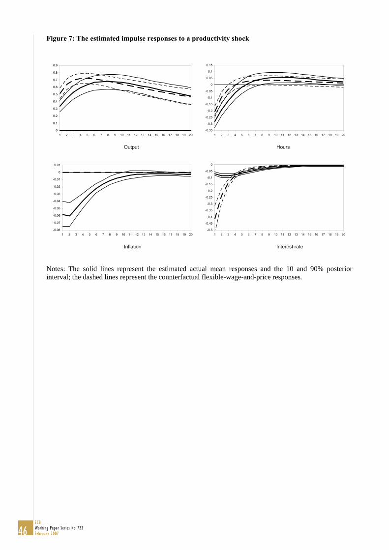
Figure 7: The estimated impulse responses to a productivity shock
Output Hours
Inflation Interest rate
0
0.1
0.2
0.3
0.4
0.5
0.6
0.7
0.8
0.9
1 2 3 4 5 6 7 8 9 10 11 12 13 14 15 16 17 18 19 20-0.35
-0.3
-0.25
-0.2
-0.15
-0.1
-0.05
0
0.05
0.1
0.15
1 2 3 4 5 6 7 8 9 10 11 12 13 14 15 16 17 18 19 20
-0.08
-0.07
-0.06
-0.05
-0.04
-0.03
-0.02
-0.01
0
0.01
1 2 3 4 5 6 7 8 9 10 11 12 13 14 15 16 17 18 19 20-0.5
-0.45
-0.4
-0.35
-0.3
-0.25
-0.2
-0.15
-0.1
-0.05
0
1 2 3 4 5 6 7 8 9 10 11 12 13 14 15 16 17 18 19 20
Notes: The solid lines represent the estimated actual mean responses and the 10 and 90% posterior interval; the dashed lines represent the counterfactual flexible-wage-and-price responses.
46ECB Working Paper Series No 722February 2007

Data appendix
Equations (1) to (14) are estimated using seven key macro-economic time series: real GDP, consumption,
investment, hours worked, real wages, prices and a short-term interest rate. The Bayesian estimation
methodology is extensively discussed in Smets and Wouters (2003). GDP, consumption and investment
are taken from the US Department of Commerce - Bureau of Economic Analysis databank. Real Gross
Domestic Product is expressed in Billions of Chained 1996 Dollars. Nominal Personal Consumption
Expenditures and Fixed Private Domestic Investment are deflated with the GDP-deflator.17 Inflation is the
first difference of the log of the Implicit Price Deflator of GDP. Hours and wages come from the BLS
(hours and hourly compensation for the NFB sector for all persons). Hourly compensation is divided by
the GDP price deflator in order to get the real wage variable. Hours are adjusted to take into account the
limited coverage of the NFB sector compared to GDP (the index of average hours for the NFB sector is
multiplied with the Civilian Employment (16 years and over)18. The aggregate real variables are
expressed per capita by dividing with the population over 16. All series are seasonally adjusted. The
interest rate is the Federal Funds Rate. Consumption, investment, GDP, wages and hours are expressed in
100 times log. The interest rate and inflation rate are expressed on a quarterly basis corresponding with
their appearance in the model (in the figures the series are translated on an annual basis).
17 We follow Altig, Christiano, Eichenbaum and Linde (2004) here. This approach avoids the positive trend in the investment
share of output that results from the decline in the relative investment expenditures deflator. A fully specified model would start from a two-sector model allowing for a separate trend in technological progress in the investment good sector. In such a two sector model, the relative price of investment and consumption goods can be used to identify the investment specific technological progress. In our one sector model, it was difficult to identify a separate deterministic trend in investment specific technology. However, there are significant short run shocks around this trend that influence investment in the short and medium run.
18 This correction is also used in Chang, Gomes and Schrofheide (2002).
47ECB
Working Paper Series No 722February 2007

Model appendix
Frank Smets and Raf Wouters
September 5, 2006
1 Decision problems of �rms and households and equilib-rium conditions
1.1 Final goods producers
The �nal good Yt is a composite made of a continuum of intermediate goods Yt(i) as in
Kimball (1995). The �nal good producers buy intermediate goods, package them into
Yt, and sell the �nal good to consumers, investors and the government in a perfectly
competitive market. They maximize pro�ts:
maxYt;Yt(i) PtYt �R 10 Pt(i)Yt(i)di
s:t:hR 10 G
�Yt(i)Yt; �pt
�dii= 1 (�f;t)
where Pt and Pt(i) are the price of the �nal and intermediate goods respectively, and G is
a strictly concave and increasing function characterised by G(1) = 1. �pt is an exogenous
process that re�ects shocks to the aggregator function that result in changes in the elas-
ticity of demand and therefore in the markup. We will constrain �pt 2 (0;1). �pt follows
the exogenous ARMA process:
ln�pt = (1� �p)ln�p + �pln�pt�1 � �p�
pt�1 + �
pt ; �
pt � N(0; �p)
Combining the �rst-order conditions with respect to Yt(i) and Yt results in:
Yt(i) = YtG0�1�Pt(i)
Pt
Z 1
0G0�Yt(i)
Yt
�Yt(i)
Ytdi
�As in Kimball (1995), the assumptions on G imply that the demand for input Yt(i) is
decreasing in its relative price, while the elasticity of demand is a positive function of the
relative price (or a negative function of the relative output).
1.2 Intermediate goods producers
Intermediate good producer i uses the following technology:
Yt(i) = "atK
st (i)
�� tLt(i)
�1�� � t� (1)
48ECB Working Paper Series No 722February 2007

where Kst (i) is capital services used in production, Lt(i) is a composite labour input and
� is a �xed cost. t respresents the labour-augmenting deterministic growth rate in the
economy and "at is total factor productivity and follows the process:
ln"at = (1� �z)ln"a + �zln"at�1 + �at ; �at � N(0; �a) (2)
The �rm�s pro�t is given by:
Pt(i)Yt(i)�WtLt(i)�RktKst (i):
where Wt is the aggregate nominal wage rate and Rkt is the rental rate on capital.
Cost minimization yields the following �rst-order conditions:
(@Lt(i)) : �t(i) (1��)t(1� �)"atKs
t (i)�Lt(i)
�� =Wt (3)
(@Kst (i)) : �t(i)
(1��)t�"atKst (i)
��1Lt(i)1�� = Rkt (4)
where �t(i) is the Lagrange multiplier associated with the production function and equals
marginal cost MCt.
Combining these FOCs and noting that the capital-labour ratio is equal across �rms
implies:
Kst =
�
1� �Wt
RktLt (5)
The marginal cost MCt is the same for all �rms and equal to:
MCt = ���(1� �)�(1��)W 1��
t Rk �t �(1��)t ("at )�1 (6)
Under Calvo pricing with partial indexation, the optimal price set by the �rm that is
allowed to re-optimise results from the following optimisation problem:
maxePt(i) Et1Xs=0
�sp�s�t+sPt�tPt+s
h ePt(i)(�sl=1��pt+l�1�1��p� )�MCt+siYt+s(i)
s:t: Yt+s(i) = Yt+sG0�1�Pt(i)Xt;sPt+s
� t+s
�where ePt(i) is the newly set price, �p is the Calvo probability of being allowed to optimiseone�s price, �t is in�ation de�ned as �t = Pt=Pt�1, [
�s�t+sPt�tPt+s
] is the nominal discount factor
for �rms (which equals the discount factor for the households that are the �nal owners of
the �rms), � t =R 10 G
0�Yt(i)Yt
�Yt(i)Ytdi and
Xt;s =
(1 for s = 0
(�sl=1��pt+l�1�
1��p� ) for s = 1; :::;1
)The �rst-order condition is given by:
Et
1Xs=0
�sp�s�t+sPt�tPt+s
Yt+s(i)
�Xt;s ePt(i) + � ePt(i)Xt;s �MCt+s� 1
G0�1(zt+s)
G0(xt+s)
G00(xt+s)
�= 0
(7)
49ECB
Working Paper Series No 722February 2007

where xt = G0�1(zt) and zt =Pt(i)Pt� t.
The aggregate price index is in this case given by:
Pt = (1� �p)Pt(i)G0�1�Pt(i)� tPt
�+ �p�
�pt�1�
1��p� Pt�1G
0�1
"��pt�1�
1��p� Pt�1� t
Pt
#(8)
1.3 Households
Household j chooses consumption Ct(j), hours worked Lt(j), bonds Bt(j), investment
It(j) and capital utilisation Zt(j), so as to maximise the following objective function:
Et
1Xs=0
�s�
1
1� �c(Ct+s(j)� �Ct+s�1)1��c
�exp
��c�11+�l
Lt+s(j)1+�l
�subject to the budget constraint:
Ct+s(j) + It+s(j) +Bt+s(j)
"btRt+sPt+s� Tt+s (9)
� Bt+s�1(j)
Pt+s+W ht+s(j)Lt+s(j)
Pt+s+Rkt+sZt+s(j)Kt+s�1(j)
Pt+s� a(Zt+s(j))Kt+s�1(j) +
Divt+sPt+s
and the capital accumulation equation:
Kt(j) = (1� �)t�1(j) + "it�1� S
�It(j)
It�1(j)
��It(j) (10)
There is external habit formation captured by the parameter �. The one-period bond
is expressed on a discount basis. "bt is an exogenous premium in the return to bonds, which
might re�ect ine¢ ciencies in the �nancial sector leading to some premium on the deposit
rate versus the risk free rate set by the central bank, or a risk premium that households
require to hold the one period bond. "bt follows the stochastic process:
ln"bt = �b ln "bt�1 + �
bt ; �
bt � N(0; �b) (11)
� is the depreciation rate, S(�) is the adjustment cost function, with S( ) = 0;
S0( ) = 0, S00(�) > 0, and "it is a stochastic shock to the price of investment relative to
consumption goods and follows an exogenous process:
ln"it = �i ln "it�1 + �
it; �
it � N(0; �i) (12)
Tt+s are lump sum taxes or subsidies and Divt are the dividends distributed by the inter-
mediate goods producers and the labour unions.
Finally, households choose the utilisation rate of capital. The amount of e¤ective cap-
ital that households can rent to the �rms is:
Kst (j) = Zt(j)Kt�1(j) (13)
The income from renting capital services is RktZt(j)Kt�1(j) , while the cost of changing
50ECB Working Paper Series No 722February 2007

capital utilisation is Pta(Zt(j))Kt�1(j):
In equilibrium households will make the same choices for consumption, hours worked,
bonds, investment and capital utilization. The �rst-order conditions can be written as
(dropping the j index):
(@Ct) �t = exp
��c�11+�l
Lt(j)1+�l
�(Ct � �Ct�1)��c (14)
(@Lt)
�1
1� �c(Ct � hCt�1)1��c
�exp
��c�11+�l
L1+�lt
�(�c�1)L�lt = ��t
W ht
Pt(15)
(@Bt) �t = �"btRtEt
��t+1�t+1
�(16)
(@It) �t = �kt "it
�1� S( It
It�1)� S0( It
It�1)ItIt�1
�+�Et
��kt+1"
it+1S
0(It+1It)(It+1It)2�
(17)
(@ �Kt) �kt = �Et
"�t+1
Rkt+1Pt+1
Zt+1 � a(Zt+1)!+ �kt+1(1� �)
#(18)
(@ut)RktPt
= a0(Zt) (19)
where �t and �kt are the Lagrange multipliers associated with the budget and capital
accumulation constraint respectively. Tobin�s Qt = �kt =�t and equals one in the absence
of adjustment costs.
1.4 Intermediate labour unions and labour packers
Households supply their homogenous labour to an intermediate labour union which di¤er-
entiates the labour services, sets wages subject to a Calvo scheme and o¤ers those labour
services to intermediate labour packers. Labour used by the intermediate goods producers
Lt is a composite made of those di¤erentiated labour services Lt(i). As with intermediate
goods, the aggregator is the one proposed by Kimball (1995). The labour packers buy the
di¤erentiated labour services, package Lt, and o¤er it to the intermediate goods producers.
The labour packers maximize pro�ts:
maxLt;Lt(i)WtLt �R 10 Wt(i)Lt(i)di
s:t:hR 10 H
�Lt(i)Lt; �wt
�dii= 1 (�l;t)
whereWt andWt(i) are the price of the composite and intermediate labour services respec-
tively, and H is a strictly concave and increasing function characterised by H(1) = 1. �wt is
an exogenous process that re�ects shocks to the aggregator function that result in changes
51ECB
Working Paper Series No 722February 2007

in the elasticity of demand and therefore in the markup. We will constrain �wt 2 (0;1).�wt follows the exogenous ARMA process:
ln�wt = (1� �w)ln�w + �wln�wt�1 � �w�wt�1 + �wt ; �wt � N(0; �w) (20)
Combining FOCs results in:
Lt(i) = LtH0�1�Wt(i)
Wt
Z 1
0H 0�Lt(i)
Lt
�Lt(i)
Ltdi
�The labour unions are an intermediate between the households and the labor packers.
Under Calvo pricing with partial indexation, the optimal wage set by the union that is
allowed to re-optimise its wage results from the following optimisation problem:
maxfWt(i)Et
1Xs=0
�sw�s�t+sPt�tPt+s
hfWt(i)(�sl=1 �
�wt+l�1��
1��w �W ht+s
iLt+s(i)
s:t: Lt+s(i) = Lt+sH0�1�Wt(i)X
wt;s
Wt+s�wt+s
�where fWt(i) is the newly set wage, �w is the Calvo probability of being allowed to optimise
one�s wage, �wt =R 10 H
0�Lt(i)Lt
�Lt(i)Ltdi and
Xwt;s =
(1 for s = 0
(�sl=1 ��wt+l�1�
1��w� ) for s = 1; :::;1
)
The �rst-order condition is given by:
Et
1Xs=0
�sw�s�t+sPt�tPt+s
Lt+s(i)
�Xwt;sfWt(i) +
�fWt(i)Xwt;s �W h
t+s
� 1
H 0�1(zwt+s)
H 0(xwt+s)
H 00(xwt+s)
�= 0
(21)
where xwt = H0�1(zwt ) and z
wt =
Wt(i)Wt
�wt .
The aggregate wage index is in this case given by:
Wt = (1� �w)fWtH0�1
"fWt�wt
Wt
#+ �w �
�wt�1�
1��w� Wt�1H
0�1
" ��wt�1�
1��w� Wt�1�wtWt
#(22)
The markup of the aggregate wage over the wage received by the households is distrib-
uted to the households in the form of dividends (see the budget constraint of households).
1.5 Government Policies
The central bank follows a nominal interest rate rule by adjusting its instrument in re-
sponse to deviations of in�ation and output from their respective target levels:
RtR�
=
�Rt�1R�
�� ���t��
�r� � YtY �t
�ry�1��� Yt=Yt�1Y �t =Y
�t�1
�r�y�rt (23)
52ECB Working Paper Series No 722February 2007

where R� is the steady state nominal rate (gross rate) and Y �t is natural output. The
parameter � determines the degree of interest rate smoothing. The exogenous monetary
policy shock �rt is determined as
ln�rt = �rln�rt�1 + �
rt (24)
The government budget constraint is of the form
PtGt +Bt�1 = Tt +BtRt
(25)
where Tt are nominal lump-sum taxes (or subsidies) that also appear in household�s
budget constraint. Government spending expressed relative to the steady state output
path "gt = Gt=(Y t) follows the process:
ln "gt = (1� �g)ln"g + �gln"gt�1 + �galn"
at � �galn"at�1 + �
gt ; �
gt � N(0; �g) (26)
where we allow for a reaction of government spending to respond to the productivity
process.
1.6 The natural output level
The natural output level is de�ned as the output in the �exible price and wage economy
without mark-up shock in prices and wages. Persistent markup shocks may therefore result
in persistent con�icts between the stabilising in�ation and the output gap and therefore
in persistent deviations of in�ation from the in�ation target.
1.7 Resource constraint
Integrating the budget constraint across households and combining with the government
budget constraint and the expressions for the dividends of intermediate goods producers
and labour unions gives the overall resource constraint:
Ct + It +Gt + a(Zt)Kt�1 = Yt (27)
2 Detrending and linearization
The model can be detrended with the deterministic trend and nominal variables can be
replaced by their real counterparts. The non-linear system is then linearised around the
stationary steady state of the detrended variables.
53ECB
Working Paper Series No 722February 2007

54ECB Working Paper Series No 722February 2007
European Central Bank Working Paper Series
For a complete list of Working Papers published by the ECB, please visit the ECB’s website(http://www.ecb.int)
691 “The yield curve as a predictor and emerging economies” by A. Mehl, November 2006.
692 “Bayesian inference in cointegrated VAR models: with applications to the demand for euro area M3” by A. Warne, November 2006.
693 “Evaluating China’s integration in world trade with a gravity model based benchmark” by M. Bussière and B. Schnatz, November 2006.
694 “Optimal currency shares in international reserves: the impact of the euro and the prospects for the dollar” by E. Papaioannou, R. Portes and G. Siourounis, November 2006.
695 “Geography or skills: What explains Fed watchers’ forecast accuracy of US monetary policy?” by H. Berger, M. Ehrmann and M. Fratzscher, November 2006.
696 “What is global excess liquidity, and does it matter?” by R. Rüffer and L. Stracca, November 2006.
697 “How wages change: micro evidence from the International Wage Flexibility Project” by W. T. Dickens, L. Götte, E. L. Groshen, S. Holden, J. Messina, M. E. Schweitzer, J. Turunen, and M. E. Ward, November 2006.
698 “Optimal monetary policy rules with labor market frictions” by E. Faia, November 2006.
699 “The behaviour of producer prices: some evidence from the French PPI micro data” by E. Gautier, December 2006.
700 “Forecasting using a large number of predictors: Is Bayesian regression a valid alternative toprincipal components?” by C. De Mol, D. Giannone and L. Reichlin, December 2006.
701 “Is there a single frontier in a single European banking market?” by J. W. B. Bos and H. Schmiedel, December 2006.
702 “Comparing financial systems: a structural analysis” by S. Champonnois, December 2006.
703 “Comovements in volatility in the euro money market” by N. Cassola and C. Morana, December 2006.
704 “Are money and consumption additively separable in the euro area? A non-parametric approach” by B. E. Jones and L. Stracca, December 2006.
705 “What does a technology shock do? A VAR analysis with model-based sign restrictions” by L. Dedola and S. Neri, December 2006.
706 “What drives investors’ behaviour in different FX market segments? A VAR-based returndecomposition analysis” by O. Castrén, C. Osbat and M. Sydow, December 2006.
707 “Ramsey monetary policy with labour market frictions” by E. Faia, January 2007.
708 “Regional housing market spillovers in the US: lessons from regional divergences in a common monetary policy setting” by I. Vansteenkiste, January 2007.
709 “Quantifying and sustaining welfare gains from monetary commitment” by P. Levine, P. McAdam and J. Pearlman, January 2007.

55ECB
Working Paper Series No 722February 2007
710 “Pricing of settlement link services and mergers of central securities depositories” by J. Tapking, January 2007.
711 “What “hides” behind sovereign debt ratings?” by A. Afonso, P. Gomes and P. Rother, January 2007.
712 “Opening the black box: structural factor models with large cross-sections” by M. Forni, D. Giannone, M. Lippi and L. Reichlin, January 2007.
713 “Balance of payment crises in emerging markets: How early were the “early” warning signals?” by M. Bussière, January 2007.
714 “The dynamics of bank spreads and financial structure” by R. Gropp, C. Kok Sørensen and J.-D. Lichtenberger, January 2007.
715 “Emerging Asia’s growth and integration: How autonomous are business cycles?” by R. Rüffer, M. Sánchez and J.-G. Shen, January 2007.
716 “Adjusting to the euro” by G. Fagan and V. Gaspar, January 2007.
717 “Discretion rather than rules? When is discretionary policy-making better than the timeless perspective?” by S. Sauer, January 2007.
718 “Drift and breaks in labor productivity” by L. Benati, January 2007.
719 “US imbalances: the role of technology and policy” by R. Bems, L. Dedola and F. Smets, January 2007.
720 “Real price wage rigidities in a model with matching frictions” by K. Kuester, February 2007.
721 “Are survey-based inflation expectations in the euro area informative?” by R. Mestre, February 2007.
722 “Shocks and frictions in US business cycles: a Bayesian DSGE approach” by F. Smets and R. Wouters, February 2007.

ISSN 1561081-0
9 7 7 1 5 6 1 0 8 1 0 0 5